rank-based lasso - e cient methods for high-dimensional
TRANSCRIPT

Journal of Machine Learning Research 21 (2020) 1-47 Submitted 2/20; Revised 10/20; Published 11/20
Rank-based Lasso - efficient methods for high-dimensionalrobust model selection
Wojciech Rejchel [email protected] of Mathematics and Computer ScienceNicolaus Copernicus UniversityChopina 12/18, 87-100 Torun, Poland
Ma lgorzata Bogdan [email protected]
Faculty of Mathematics and Computer Science
University of Wroc law
Joliot-Curie 15, 50-383 Wroc law, Poland
and
Department of Statistics
Lund University
Tycho Brahes vag 1, Lund, Sweden
Editor: Garvesh Raskutti
Abstract
We consider the problem of identifying significant predictors in large data bases, where theresponse variable depends on the linear combination of explanatory variables through anunknown monotonic link function, corrupted with the noise from the unknown distribution.We utilize the natural, robust and efficient approach, which relies on replacing values ofthe response variables by their ranks and then identifying significant predictors by usingwell known Lasso. We provide new consistency results for the proposed procedure (called,,RankLasso”) and extend the scope of its applications by proposing its thresholded andadaptive versions. Our theoretical results show that these modifications can identify the setof relevant predictors under a wide range of data generating scenarios. Theoretical resultsare supported by the simulation study and the real data analysis, which show that ourmethods can properly identify relevant predictors, even when the error terms come fromthe Cauchy distribution and the link function is nonlinear. They also demonstrate thesuperiority of the modified versions of RankLasso over its regular version in the case whenpredictors are substantially correlated. The numerical study shows also that RankLassoperforms substantially better in model selection than LADLasso, which is a well establishedmethodology for robust model selection.
Keywords: Lasso, Model Selection, Ranks, Single Index Model, Sparsity, U -statistics
1. Introduction
Model selection is a fundamental challenge when working with large-scale data sets, wherethe number of predictors exceeds significantly the number of observations. In many practicalproblems finding a small set of significant predictors is at least as important as accurateestimation or prediction. Among many approaches to high-dimensional model selection one
c©2020 Wojciech Rejchel and Ma lgorzata Bogdan.
License: CC-BY 4.0, see https://creativecommons.org/licenses/by/4.0/. Attribution requirements are providedat http://jmlr.org/papers/v21/20-120.html.

Rejchel and Bogdan
can distinguish a large group of methods based on penalized estimation (Hastie et al., 2001;Buhlmann and van de Geer, 2011). Under the linear regression model
Yi = β′Xi + εi, i = 1, . . . , n,
where Yi ∈ R is a response variable, Xi ∈ Rp is a vector of predictors, β ∈ Rp is the vectorof model parameters and εi is a random error, the penalized model selection approachesusually recommend estimating the vector of regression coefficients β by
β = arg minβ∈Rp
n∑i=1
(Yi − β′Xi)2 + Pen(β), (1)
where∑n
i=1(Yi− β′Xi)2 is the quadratic loss function measuring the model fit and Pen(β)
is the penalty on the model complexity. The main representative of these methods is Lasso(Tibshirani, 1996), which uses the l1-norm penalty. The properties of Lasso in model selec-tion, estimation and prediction are deeply investigated, e.g. in Meinshausen and Buhlmann(2006); Zhao and Yu (2006); Zou (2006); van de Geer (2008); Bickel et al. (2009); Ye andZhang (2010); Buhlmann and van de Geer (2011); Huang and Zhang (2012); Su et al. (2017);Tardivel and Bogdan (2018). These articles discuss the properties of Lasso in the contextof linear or generalized linear models and their results hold under specific assumptions onthe relationship between the response and explanatory variables and/or the distribution ofthe random errors. However, it is quite common that a complex data set does not satisfythese assumptions or they are difficult to verify. In such cases it is advised to use ,,robust”methods of model selection.
In this paper we consider the single index model
Yi = g(β′Xi, εi), i = 1, . . . , n, (2)
where g is unknown monotonic link function. Thus, we suppose that predictors influencethe response variable through the link function g of the scalar product β′Xi. However, wemake no assumptions on the form of the link function g (except being monotonic) nor onthe distribution of the error term εi. Specifically, we do not assume the existence of theexpected value of εi.
The goal of model selection is the identification of the set of relevant predictors
T = 1 ≤ j ≤ p : βj 6= 0. (3)
The literature on the topic of robust model selection is quite considerable and the com-prehensive review can be found e.g. in Wu and Ma (2015). Many of the existing methodssuppose that the linear model assumption is satisfied and consider the robustness with re-spect to the noise. Here the most popular approaches rely on replacing the regular quadraticloss function with the loss function, which is more robust with respect to outliers, like e.g.the absolute value or Huber loss functions (Huber, 1964). Model selection properties of thepenalized regression procedures with such robust loss functions were investigated, amongothers, in Wang et al. (2007); Gao and Huang (2010); Belloni and Chernozhukov (2011);Wang et al. (2012); Wang (2013); Fan et al. (2014); Peng and Wang (2015); Zhong et al.(2016); Avella-Medina and Ronchetti (2018). Among these methods one can mention the
2
Rank-based Lasso
approach of Johnson and Peng (2008); Johnson (2009), where the loss function is expressedin terms of residual ranks. On the other hand, the issues of model selection in misspecifiedmodels were discussed in e.g. Lu et al. (2012); Lv and Liu (2014), while robustness withrespect to the unknown link function g in the single index model (2) was discussed, forinstance, in Kong and Xia (2007); Zeng et al. (2012); Alquier and Biau (2013); Plan andVershynin (2016); Cheng et al. (2017). In particular, Plan and Vershynin (2016) proposeda procedure, which can estimate the parameter β with accuracy to the multiplicative con-stant, when predictors X are Gaussian and EY 2 < ∞. Their approach was extended toincorporate different loss functions (Genzel, 2017), non-Gaussian predictors (Yang et al.,2017a,b; Wei et al., 2019) and to high-dimensional varying index coefficient models (Naet al., 2019). The extensions in (Yang et al., 2017a,b; Wei et al., 2019; Na et al., 2019)are based on Stein’s lemma (Stein, 1972; Stein et al., 2004) and the proposed solutionsdepend on the distribution of predictors, which is assumed to be known. Additionally, allthese works require some moment assumptions on Y , which precludes application of thismethodology, when the errors have a heavy-tailed distribution, like e.g., Cauchy or somecases of log-normal distribution.
Penalized robust model selection procedures for single-index models with heavy tailederrors were developed e.g. in Zhu and Zhu (2009); Song and Ma (2010); Wang and Zhu(2015); Zhong et al. (2016); Rejchel (2017b,a), where their desired statistical propertiesare confirmed. However, the application of procedures based on robust loss functions (e.g.piecewise-linear) in the context of the analysis of large data sets is often limited due to theircomputational complexity and/or the need of the development of dedicated optimizationalgorithms. For instance, in Sections 3 and 4 we consider the Least Absolute DeviationLasso (LADLasso) estimator (Wang et al., 2007; Belloni and Chernozhukov, 2011; Fanet al., 2014), which turns out to be computationally very slow even for moderate dimensionexperiments.
In the current paper we consider an alternative approach for identifying important pre-dictors in the single index model. Our method does not require knowledge of the distributionof predictors or any moment assumptions on the error distribution. Moreover, it is com-putationally fast and can work efficiently with complex high-dimensional data sets. Ourprocedure is very simple and relies on replacing actual values of the response variables Yiby their centred ranks. Ranks Ri are defined as
Ri =n∑j=1
I(Yj ≤ Yi), i = 1, . . . , n, (4)
where I(·) is the indicator function. Next, we identify significant predictors by simply solvingthe following Lasso problem;
RankLasso: θ = arg minθ∈Rp
Q(θ) + λ |θ|1 , (5)
where
Q(θ) =1
2n
n∑i=1
(Ri/n− 0.5− θ′Xi
)2. (6)
This procedure does not require any dedicated algorithm and can be executed using efficientimplementations of Lasso in ,,R” (R Development Core Team, 2017) packages: ,,lars” (Efron
3

Rejchel and Bogdan
et al., 2004) or ,,glmnet” (Friedman et al., 2010). Technically, RankLasso was introducedbefore in Zhu and Zhu (2009); Wang and Zhu (2015), who used a slightly more complicateddefinition, which makes it difficult to notice the relationship with ranks.
Replacing values of response variables by their ranks is a well-known approach in non-parametric statistics and leads to robust procedures. The premier examples of a rankapproach are the Wilcoxon test, that is a widely used alternative to the Student’s t-test, orthe Kruskall-Wallis ANOVA test. While the rank tests often have a low power for a smallnumber of observations, they can achieve high efficiency for large sample sizes. As shown inZak et al. (2007); Bogdan et al. (2008), this carries over to the high efficiency of identifyingimportant predictors in the sparse high-dimensional regression models, where the numberof true nonzero regression coefficients is much smaller than the sample size n.
The methodology proposed in Zak et al. (2007); Bogdan et al. (2008) relies on minimiza-tion of the rank version of the Bayesian Information Criterion, which in principle is N-Phard. While the heuristics based on the greedy search algorithms can in some cases identifyapproximately optimal models, they are not reliable in the case when predictors are highlycorrelated. Instead, RankLasso is based on a convex optimization algorithm, which can beeasily solved even when p >> n and the explanatory variables are highly correlated.
One of the disadvantages of the rank approach is the loss of information about theshape of the link function. Therefore, RankLasso cannot be directly used to build thepredictive model for the response variable. In the case when errors are subgaussian, suchpredictive models can be constructed using e.g. the estimation method for the single-indexmodel proposed in Balabdaoui et al. (2019), which can be also extended to the generalerror distribution by replacing the L2-loss with the robust loss functions (say, the L1 or theHuber loss functions). However, this method can handle only a small number of predictors.In this article we demonstrate that significant predictors can be appropriately fished outfrom the large data base by simple modifications of RankLasso.
Specifically, in Subsection 2.2 we provide the definition of the parameter θ0, that isestimated by RankLasso, and discuss its relationship to the true vector of regression coeffi-cients β. It turns out that under certain standard assumptions, the support of θ0 coincideswith the support of β and the methods based on ranks can identify the set of relevant pre-dictors. However, similarly as in the case of regular Lasso, RankLasso can identify the truemodel only under very restrictive ”irrepresentable conditions” on the correlations betweenpredictors and the sparsity of the vector of regression coefficients, see e.g. Zhao and Yu(2006); van de Geer and Buhlmann (2009); Wang and Zhu (2015). An intuitive explanationof these problems with model selection relates to the role of a tuning parameter λ. Namely,to obtain good model selection properties the parameter λ needs to be sufficiently large todiscard irrelevant predictors. However, large λ leads to a large bias of Lasso estimators.In the result a non-explained effect of relevant predictors is intercepted by even slightlycorrelated variables, which leads to early false discoveries along the Lasso path and sub-stantial difficulties with identification of the true model, see e.g. Su et al. (2017). Thisproblem can be solved by using smaller value of the tuning parameter. An illustration ofthis phenomenon can be found in Weinstein et al. (2020), where it is shown that the or-dering of estimated regression coefficients does not remain constant along the Lasso path.It turns out that the small mean squared error of Lasso estimates is typically obtainedfor a relatively small value of λ, where the coefficients corresponding to true discoveries
4
Rank-based Lasso
become larger than the ones for false discoveries, which appeared earlier on the Lasso path(Weinstein et al., 2020). Therefore, while regular Lasso usually cannot identify the truemodel for any selection of the tuning parameter λ, there often exists a range of λ values,which provide a good separation between the estimated regression coefficients of true andfalse predictors, see e.g. Ye and Zhang (2010); Buhlmann and van de Geer (2011); Tardiveland Bogdan (2018); Weinstein et al. (2020). In Weinstein et al. (2020) a detailed powercomparison of two model selection procedures:
• Lasso: select j : βLassoj (λ) 6= 0,
• Thresholded Lasso: select j : |βLassoj (λ)| > t for some threshold t > 0
is performed in the situation when the covariates are independent gaussian variables. Thisanalysis shows that appropriately thresholded Lasso with the tuning parameter selectedby cross-validation yields much higher power than regular Lasso for the same expectednumber of false discoveries and can identify the true model under much weaker regularityassumptions. Also, cross-validated Lasso estimators are often good candidates for the firststep estimates for adaptive Lasso (Zou, 2006).
In this paper we use the above ideas and extend the scope of applications of RankLassoby proposing its thresholded and adaptive versions. In the case of standard Lasso similarmodifications were introduced and discussed e.g. in Zou (2006); Candes et al. (2008); Zhou(2009); Tardivel and Bogdan (2018); Weinstein et al. (2020). We prove that the proposedmodifications of RankLasso are model selection consistent in the model (2) under muchweaker conditions than the ones provided in Wang and Zhu (2015) for regular RankLasso.More specifically, our results show that the modifications of RankLasso can identify thetrue model for any unknown monotonic link function and any unknown distribution of theerror term and under much weaker restrictions on the design matrix and the signal sparsitythan in the case of regular RankLasso. These theoretical results require a substantial mod-ification of the proof techniques as compared to the similar results for regular Lasso. It isrelated to the fact that ranks are dependent, so (6) is a sum of dependent random variables.In Subsection 2.4 we describe how this problem can be overcome with the application ofthe theory of U -statistics. We also present extensive numerical results illustrating that themodifications of RankLasso can indeed properly identify relevant predictors, when the linkfunction is not linear, error terms come from, say, the Cauchy distribution and predictorsare substantially correlated. Specifically, it can be observed that, contrary to regular Ran-kLasso, the proposed modifications can control the number of false discoveries and achievea high power under strongly correlated designs. These results also show that RankLassocompares favorably with LADLasso, which is a well established methodology for robustmodel selection (Wang et al., 2007; Belloni and Chernozhukov, 2011; Fan et al., 2014).
The paper is organized as follows: in Section 2 we present theoretical results on the modelselection consistency of RankLasso and its modifications. In Subsection 2.2 we discuss therelationship between β and the parameter estimated by RankLasso. We show that ourapproach is able to identify the support of β in the single index model. In Subsection 2.3we consider properties of estimators in the high-dimensional scenario, where the number ofpredictors can be much larger than the sample size. We establish nonasymptotic boundson the estimation error and separability of RankLasso. We use these results to prove model
5

Rejchel and Bogdan
selection consistency of thresholded and weighted RankLasso. In Subsection 2.4 we brieflydraw a road map to the proofs of main results. Sections 3 and 4 are devoted to experimentsthat illustrate the properties of rank-based estimators on simulated and real data sets,respectively. The paper is concluded in Section 5. The proofs of main and auxiliary resultsare relegated to the appendix. We also place in the appendix results for the low-dimensionalcase, where the number of predictors is fixed and the sample size diverges to infinity. Inthis case we provide the necessary and sufficient conditions for model selection consistencyof RankLasso and much weaker sufficient conditions for thresholded and weighted versionsof RankLasso.
2. Model selection properties of RankLasso and its modifications
In this section we provide theoretical results concerning model selection as well as estimationproperties of RankLasso and its thresholded and weighted versions. We start with specifyingthe assumptions on our model.
2.1 Assumptions and notation
Consider the single index model (2). In this paper we assume that the design matrix X andthe vector of the error terms ε satisfy the following assumptions.
Assumption 1 We assume that (X1, ε1), . . . , (Xn, εn) are i.i.d. random vectors such thatthe distribution of X1 is absolutely continuous and X1 is independent of the noise variable ε1.Additionally, we assume that EX1 = 0, H = EX1X
′1 is positive definite and Hjj = 1 for
j = 1, . . . , p.
The single index model (2) does not allow to estimate an intercept and can identifyβ only up to a multiplicative constant, because any shift or scale change in β′Xi can beabsorbed by g. However, in many situations RankLasso can properly identify the supportT of β. In this paper we will prove this fact under the following assumption.
Assumption 2 We assume that for each θ ∈ Rp the conditional expectation E(θ′X1|β′X1)exists and
E(θ′X1|β′X1) = dθβ′X1
for a real number dθ ∈ R.
Assumption 2 is a standard condition in the literature on the single index model or onthe model misspecification, see e.g. Brillinger (1983); Ruud (1983); Li and Duan (1989);Zhu and Zhu (2009); Wang and Zhu (2015); Zhong et al. (2016); Kubkowski and Mielniczuk(2017). It is always satisfied in the simple regression models (i.e. when X1 ∈ R), whichare often used for initial screening of explanatory variables, see e.g. Fan and Lv (2008).It is also satisfied whenever X1 comes from the elliptical distribution, like the multivariatenormal distribution or multivariate t-distribution. The interesting paper Hall and Li (1993)advocates that Assumption 2 is a nonrestrictive condition when the number of predictorsis large, which is the case that we focus on in the paper. In the experimental section of thisarticle we show that RankLasso, proposed here, is able to identify the support of β also
6

Rank-based Lasso
when the columns of the design matrix contain genotypes of independent Single NucleotidePolymorphisms, whose distribution is not symmetric and clearly does not belong to theelliptical distribution.
The identifiability of the support of β by the rank procedure requires also the assump-tions on the monotonicity of the link function g and the cumulative distribution function ofY1. The following Assumption 3, which combines Assumptions 1 and 2 and the monotonicityassumptions, will be used in most of theoretical results in this article.
Assumption 3 We assume that the design matrix and the error term satisfy Assumptions1 and 2, the cumulative distribution function F of the response variable Y1 is increasingand g in (2) is increasing with respect to the first argument.
In this paper we will use the following notation:- X = (X1, X2, . . . , Xn)′ is the (n× p)-matrix of predictors,- X = 1
n
∑ni=1Xi,
- Zi = (Xi, Yi), i = 1, . . . , n,- T ′ = 1, . . . , p \ T is a complement of T ,- XT is a submatrix of X, with columns whose indices belong to the support T of β, see (3),- θT is a restriction of a vector θ ∈ Rp to the indices from T,- p0 is the number of elements in T,
- the lq-norm of a vector is defined as |θ|q =(∑p
j=1 |θj |q)1/q
for q ∈ [1,∞].
2.2 Identifying the support of β
RankLasso does not estimate β, but the vector
θ0 = arg minθ∈Rp
EQ(θ), (7)
where Q(θ) is defined in (6). Since H is positive definite, the minimizer θ0 is unique and isgiven by the formula
θ0 =1
n2H−1
(E
n∑i=1
RiXi
). (8)
Now, using the facts that
n∑i=1
RiXi =n∑i=1
n∑j=1
I(Yj ≤ Yi)Xi =∑i 6=j
I(Yj ≤ Yi)Xi +n∑i=1
Xi (9)
and that EXi = 0, we can write
θ0 =n− 1
nH−1µ, (10)
where µ = E [I(Y2 ≤ Y1)X1] is the expected value of the U -statistic
A =1
n(n− 1)
∑i 6=j
I(Yj ≤ Yi)Xi . (11)
In the next theorem we state the relation between θ0 and β.
7

Rejchel and Bogdan
Theorem 1 Consider the model (2). If Assumptions 1 and 2 are satisfied, then
θ0 = γββ
with
γβ =n−1n β′µ
β′Hβ=
n−1n Cov(F (Y1), β′X1)
β′Hβ, (12)
where F is a cumulative distribution function of a response variable Y1.Additionally, if F is increasing and g is increasing with respect to the first argument,
then γβ > 0, so the signs of β coincide with the signs of θ0 and
T = j : βj 6= 0 = j : θ0j 6= 0. (13)
We can apply Theorem 1 to the additive model Yi = g1(β′Xi) + εi with an increasingfunction g1. Then, under Assumptions 1 and 2, θ0 = γββ with γβ > 0 if, for example, thesupport of the noise variable is a real line. Moreover, since the procedure based on ranks isinvariant with respect to increasing transformations of response variables the same appliesto the model Yi = g2(β′Xi + εi) with an increasing function g2.
2.3 High-dimensional scenario
In this subsection we consider properties of the RankLasso estimator and its modificationsin the case where the number of predictors can be much larger than the sample size. Toobtain the results of this subsection we need the additional condition:
Assumption 4 We suppose that the vector of significant predictors (X1)T is subgaussianwith the coefficient τ0 > 0, i.e. for each u ∈ Rp0 we have E exp(u′(X1)T ) ≤ exp(τ2
0u′u/2).
Moreover, the irrelevant predictors are univariate subgaussian, i.e. for each a ∈ R andj /∈ T we have E exp(aX1j) ≤ exp(τ2
j a2/2) for positive numbers τj . Finally, we denote
τ = max(τ0, τj , j /∈ T ).
We need subgaussianity of the vector of predictors to obtain exponential inequalities inthe proofs of the main results in this subsection. This condition is a standard assumptionwhile working with random predictors (Raskutti et al., 2010; Huang et al., 2013; Buhlmannand van de Geer, 2015) in high-dimensional models.
2.3.1 Estimation error and separability of RankLasso
Model selection consistency of RankLasso in the high-dimensional case was proved in Wangand Zhu (2015, Theorem 2.1). However, this result requires the stringent irrepresentablecondition. Moreover, it is obtained under the polynomial upper bound on the dependencyof p on n and provides only a rough guidance of selection of the tuning parameter λ. Inour article we concentrate on estimation consistency of RankLasso, which paves the wayfor model selection consistency of the weighted and thresholded versions of this method.Compared to the asymptotic results of Wang and Zhu (2015) our results are stated inthe form of non-asymptotic inequalities, they do not require the irrepresentable condition,allow for the exponential increase of p as a function of n and provide a precise guidance onselection of regularization parameter λ.
8

Rank-based Lasso
We start with introducing the cone invertibility factor (CIF), that plays an importantrole in investigating properties of estimators based on the Lasso penalty (Ye and Zhang,2010). In the case n > p one usually uses the minimal eigenvalue of the matrix X ′X/n toexpress the strength of correlations between predictors. Obviously, in the high-dimensionalscenario this value is equal to zero and the minimal eigenvalue needs to be replaced bysome other measure of predictors interdependency, which would describe the potential ofconsistent estimation of model parameters.
Let T be the set of indices corresponding to the support of the true vector β and let θTand θT ′ be the restrictions of the vector θ ∈ Rp to the indices from T and T ′, respectively.Now, for ξ > 1 we consider a cone
C(ξ) = θ ∈ Rp : |θT ′ |1 ≤ ξ|θT |1 .
In the case when p >> n three different characteristics measuring the potential for con-sistent estimation of the model parameters have been introduced:- the restricted eigenvalue (Bickel et al., 2009):
RE(ξ) = inf0 6=θ∈C(ξ)
θ′X ′Xθ/n
|θ|22,
- the compatibility factor (van de Geer, 2008):
K(ξ) = inf06=θ∈C(ξ)
p0θ′X ′Xθ/n
|θT |21,
- the cone invertibility factor (CIF, (Ye and Zhang, 2010)): for q ≥ 1
Fq(ξ) = inf06=θ∈C(ξ)
p1/q0 |X ′Xθ/n|∞
|θ|q.
Relations between the above quantities are discussed, for instance, in van de Geer andBuhlmann (2009); Ye and Zhang (2010); Huang et al. (2013). The fact that these conditionsare much weaker than irrepresentable conditions is also established there.
In this article we will use CIF, since this factor allows for a sharp formulation of con-vergency results for all lq norms with q ≥ 1, see Ye and Zhang (2010, Section 3.2). Thepopulation (non-random) version of CIF is given by
Fq(ξ) = inf06=θ∈C(ξ)
p1/q0 |Hθ|∞|θ|q
,
where H = EX1X′1. The key property of the random and the population versions of CIF,
Fq(ξ) and Fq(ξ), is that, in contrast to the smallest eigenvalues of matrices X ′X/n and H,they can be close to each other in the high-dimensional setting, see Huang et al. (2013,Lemma 4.1) or van de Geer and Buhlmann (2009, Corollary 10.1). This fact is used in theproof of Theorem 2 (given below).
In the simulation study in Section 3 we consider predictors, which are independent orequi-correlated, i.e. Hjj = 1 and Hjk = b for j 6= k and b ∈ [0, 1). In this case the smallesteigenvalue of H is 1− b. For ξ > 1 and q ≥ 2 we can bound CIF from below by
Fq(ξ) ≥ (1 + ξ)−1p1/q−1/20 (1− b) ,
9

Rejchel and Bogdan
which illustrates that CIF diminishes with the increase of p0 and b. Also, in the case whenH = I and q =∞, Fq(ξ) = 1, independently of ξ or p0.
The next result describes the estimation accuracy of RankLasso.
Theorem 2 Let a ∈ (0, 1), q ≥ 1 and ξ > 1 be arbitrary. Suppose that Assumptions 3 and 4are satisfied. Moreover, suppose that
n ≥ K1p20τ
4(1 + ξ)2 log(p/a)
F 2q (ξ)
(14)
and
λ ≥ K2ξ + 1
ξ − 1τ2
√log(p/a)
κn, (15)
where K1,K2 are universal constants and κ is the smallest eigenvalue of the correlationmatrix between the true predictors HT = (Hjk)j,k∈T . Then there exists a universal constantK3 > 0 such that with probability at least 1−K3a we have
|θ − θ0|q ≤4ξp
1/q0 λ
(ξ + 1)Fq(ξ). (16)
Besides, if X1 has a normal distribution N(0, H), then κ and τ can be dropped in (14) and (15).
In Theorem 2 we provide the bound for the estimation error of RankLasso. This resultalso provides the conditions for the estimation consistency of RankLasso, which can beobtained by replacing a with a sequence an, that decreases not too fast and selecting theminimal λ = λn satisfying the condition (15). The consistency holds in the high-dimensionalscenario, i.e. the number of predictors can be significantly greater than the sample size.Indeed, the consistency in the l∞-norm holds e.g. when p = exp(nα1), p0 = nα2 , a =exp(−nα1), where α1 +2α2 < 1, and λ is equal to the right-hand side of the inequality (15),provided that F∞(ξ) and κ are bounded from below (or slowly converging to 0) and τ isbounded from above (or slowly diverging to ∞).
Theorem 2 is an analog of Theorem 3 in Ye and Zhang (2010), which refers to the linearmodel with noise variables having a finite variance. Similar results for quantile regression,among others for LADLasso, can be found in Belloni and Chernozhukov (2011, Theorem 2)and Wang (2013, Theorem 1). These results do not require existence of the noise variance,but impose some restrictions on the conditional distribution of Y1 given X1, cf. Belloni andChernozhukov (2011, Assumption D.1) or Wang (2013, the condition (13)).
In Alquier and Biau (2013); Plan and Vershynin (2016); Yang et al. (2017a,b); Weiet al. (2019) the results similar to Theorem 2 were obtained also in the context of the singleindex model. However, all these articles impose some moment restrictions on Y and thuscannot handle heavy-tailed noise distributions. Besides, in Alquier and Biau (2013) the linkfunction are predictors are assumed to be bounded, while the methods analyzed in Planand Vershynin (2016); Yang et al. (2017a,b); Wei et al. (2019) require the knowledge of thepredictors’ distribution. In the case of RankLasso we were able to prove Theorem 2 undera non-restrictive Assumption 2 on the distribution of predictors and without assumptionson existence of moments of Y or the noise variable ε.
10

Rank-based Lasso
The following corollary is an easy consequence of Theorem 2. It states that underassumptions of Theorem 2 RankLasso can assymptotically separate relevant and irrelevantpredictors.
Corollary 3 Suppose that conditions of Theorem 2 are satisfied for q = ∞. Let θ0min =
minj∈T|θ0j |. If θ0
min ≥8ξλ
(ξ+1)F∞(ξ) , then
P(∀j∈T,k/∈T |θj | > |θk|
)≥ 1−K3a .
The separation of predictors by RankLasso given in Corollary 3 is a very importantproperty. It will be used to prove model selection consistency of the thresholded andweighted RankLasso in the next part of the paper.
Finally, we discuss the condition of Corollary 3 that θ0min cannot be too small, i.e.
θ0min ≥
8ξλ(ξ+1)F∞(ξ) . Using Theorem 1 we know that θ0 = γββ and γβ > 0, so this condition
refers to the strength of the true parameter β and requires that
minj∈T|βj | ≥
8ξλ
γβ(ξ + 1)F∞(ξ). (17)
Compared to the similar condition for regular Lasso in the linear model, the denominatorcontains an additional factor γβ. This number is usually smaller than one, so RankLassoneeds larger sample size to work well. This phenomenon is typical for the single-indexmodel, where the similar restrictions hold for competitive methods like e.g. LADLasso.
Below we provide a simplified version of Theorem 2, formulated under the assumptionthat F∞(ξ) and κ are lower bounded and τ is upper bounded. This formulation will be usedin the following subsection to increase the transparency of the results on model selectionconsistency of weighted and thresholded RankLasso.
Corollary 4 Let a ∈ (0, 1) be arbitrary. Suppose that Assumptions 3 and 4 are satisfied.Moreover, assume that there exist ξ0 > 1 and constants C1 > 0 and C2 < ∞ such thatκ ≥ C1, F∞(ξ0) ≥ C1 and τ ≤ C2. If
n ≥ K1p20 log(p/a)
and
λ ≥ K2
√log(p/a)
n,
then
P(|θ − θ0|∞ ≤ 4λ/C1
)≥ 1−K3a , (18)
where the constants K1 and K2 depend only on ξ0, C1, C2 and K3 is a universal constantprovided in Theorem 2.
11

Rejchel and Bogdan
2.3.2 Modifications of RankLasso
The main drawback of RankLasso considered in Subsection 2.3.1 is that it can recover thetrue model only if the restrictive irrepresentable condition is satisfied. If this condition doesnot hold, then RankLasso can achieve a high power only by including a large number ofirrelevant predictors. In Theorems 5 and 7 we state that this problem can be overcomeby the application of weighted or thresholded versions of RankLasso. In both cases werely on the initial RankLasso estimator θ of θ0, which is estimation consistent under theassumptions of Theorem 2 or Corollary 4. Theorems 5 and 7 are stated under simplifiedassumptions of Corollary 4. We have decided to establish them in these versions to makethis subsection more communicable.
First, we consider thresholded RankLasso, which is denoted by θth and defined as
θthj = θjI(|θj | ≥ δ), j = 1, . . . , p, (19)
where θ is the RankLasso estimator given in (5) and δ > 0 is a threshold. Theorem 5provides the conditions under which this procedure is model selection consistent.
Theorem 5 We assume that Corollary 4 holds and that the sample size and the tuningparameter λ for RankLasso are selected according to Corollary 4. Moreover, suppose thatθ0min = min
j∈T|θ0j | is such that it is possible to select the threshold δ so as
θ0min/2 ≥ δ > K4λ,
where K4 = 4/C1 is the constant from (18). Then it holds
P(T th = T
)≥ 1−K3a,
where K3 is the universal constant from Theorem 2 and T th = 1 ≤ j ≤ p : θthj 6= 0 is theestimated set of relevant predictors by thresholded RankLasso.
Remark 6 Theorem 5 illustrates that thresholded RankLasso has the potential for identi-fying the support of β under rather mild regularity conditions. This means that under theseconditions the sequence of nested models based on the ranking provided by RankLasso esti-mates contains the true model. In the simulation study in Section 3 we select the thresholdsuch that thresholded RankLasso returns the same number nonzero coefficients as weightedRankLasso, whose consistency is proved in Theorem 7 (below). However, there exists avariety of other methods, which could be used to select one of these nested models, includ-ing e.g. the rank version of the modified Bayesian Information Criterion proposed anddiscussed in Zak et al. (2007); Bogdan et al. (2008). Another plausible approach for iden-tifying true predictors while controlling the false discovery rate at any given level could relyon the application of the knockoffs methodology of Barber and Candes (2015); Candes et al.(2018), based on the RankLasso Coefficient Difference statistics. Concerning the selectionof the value of the tuning parameter λ, the results of Weinstein et al. (2020) for regularLasso and our simulations for RankLasso, suggest that selection of the tuning parameter λby cross-validation usually leads to the satisfactory performance of thresholded versions of
12

Rank-based Lasso
Lasso. Here one could also mention the work of Pokarowski and Mielniczuk (2015) in thecontext of regular multiple regression, who suggest selecting λ such that the related sequenceof nested regression models allows to obtain a minimal value of the respective informationcriterion.
Next, we consider the weighted RankLasso that minimizes
Q(θ) + λa
p∑j=1
wj |θj |, (20)
where λa > 0 and weights are chosen in the following way: for arbitrary number K > 0 andthe RankLasso estimator θ from the previous subsection we have wj = |θj |−1 for |θj | ≤ λa,and wj ≤ K, otherwise.
The next result describes properties of the weighted RankLasso estimator.
Theorem 7 We assume that Corollary 4 holds and that the sample size and the tuningparameter λ for RankLasso are selected according to Corollary 4. Let λa = K4λ, whereK4 = 4/C1 is from (18). Additionally, we suppose that the signal strength and sparsitysatisfy θ0
min/2 > λa and p0λ ≤ K5, where K5 is sufficiently small constant. Then withprobability at least 1−K6a there exists a global minimizer θa of (20) such that θaT ′ = 0 and
|θaT − θ0T |1 ≤ K7p0λ , (21)
where K6 and K7 are the constants depending only on K1, . . . ,K5 and the constant K, thatis used in the definition of weights.
In Fan et al. (2014, Corollary 1) the authors considered weighted Lasso with the absolutevalue loss function in the linear model. Thus, this procedure is robust with repect to thedistribution of the noise variable. However, working with the absolute value loss functionthey need that, basically, the density of the noise is Lipschitz in a neighbourhood of zero(Fan et al., 2014, Condition 1). Our thresholded and weighted RankLasso does not requiresuch restrictions. Besides, Theorems 5 and 7 confirm that the proposed procedures workswell in model selection in the single index model (2).
It can be seen in the proof of Theorem 7 that K7 is an increasing function of K, thatoccurs in the construction of weights. It is intuitively clear, because weights wj ≤ Kusually correspond (by Corollary 3) to significant predictors. Therefore, increasing K weshrink coordinates of the estimator, so the bias increases. This fact is described in (21).
2.4 Road map to proofs of main results
In the paper we study properties of the RankLasso estimator and its thresholded andweighted modifications. These estimators are obtained by minimization of the risk Q(θ)defined in (6) and the penalty. Therefore, the analysis of model selection properties ofrank-based estimators is based on investigating these two terms. The penalty term can behandled using standard methods for regular Lasso. However, the analysis of the risk Q(θ)is different, because it is the sum of dependent variables. In this subsection we show that
13

Rejchel and Bogdan
the theory of U -statistics (Hoeffding, 1948; Serfling, 1980; de la Pena and Gine, 1999) playsa prominent role in studying properties of the risk Q(θ).
Consider the key object that is the derivative of the risk at the true point θ0
∇Q(θ0) = − 1
n2
n∑i=1
RiXi +1
2n
n∑i=1
Xi +1
n
n∑i=1
XiX′iθ
0. (22)
The second and third terms in (22) are sums of independent random variables, but the firstone is a sum of dependent random variables. Using (9) we can express (22) as
−n− 1
nA+
n− 2
2n2
n∑i=1
Xi +1
n
n∑i=1
XiX′iθ
0 (23)
where a U -statistic A is defined in (11) and has the kernel
f(zi, zj) =1
2[I(yj ≤ yi)xi + I(yi ≤ yj)xj ] . (24)
To handle (23) we will use tools for sums of independent random variables as well as theU -statistics theory. Namely, we use exponential inequalities for sums of independent andunbounded random variables from van de Geer (2016, Corollary 8.2) and its version forU -statistics given in Lemma 14 in the appendix.
3. Simulation study
In this section we present results of the comparative simulation study verifying the propertiesof RankLasso and its thresholded and adaptive versions in model selection.
We consider the moderate dimension setup, where the number of explanatory variablesp increases with n according to the formula p = 0.01n2. More specifically, we consider thefollowing pairs (n, p) : (100, 100), (200, 400), (300, 900), (400, 1600). For each of thesecombinations we consider three different values of the sparsity parameter p0 = #j : βj 6=0 ∈ 3, 10, 20.
In three of our simulation scenarios the rows of the design matrix are generated asindependent random vectors from the multivariate normal distribution with the covariancematrix Σ defined as follows- for the independent case Σ = I,- for the correlated case Σii = 1 and Σij = 0.3 for i 6= j.
In one of the scenarios the design matrix is created by simulating the genotypes of p in-dependent Single Nucleotide Polymorphisms (SNPs). In this case the explanatory variablescan take only three values: 0 for the homozygote for the minor allele (genotype a,a),1 for the heterozygote (genotype a,A) and 2 for the homozygote for the major allele(genotype A,A). The frequencies of the minor allele for each SNP are independentlydrawn from the uniform distribution on the interval (0.1, 0.5). Then, given the frequencyπj for j-th SNP, the explanatory variable Xij has the distribution: P (Xij = 0) = π2
j ,
P (Xij = 1) = 2πj(1− πj) and P (Xij = 2) = (1− πj)2.The full description of the simulation scenarios is provided below:
- Scenario 1Y = Xβ + ε,
14

Rank-based Lasso
where X matrix is generated according to the independent case, β1 = . . . = βp0 = 3 and theelements of ε = (ε1, . . . , εn) are independently drawn from the standard Cauchy distribu-tion,- Scenario 2 - the regression model, values of regression coefficients and ε are as in Sce-nario 1, design matrix contains standardized versions of genotypes of p independent SNPs,- Scenario 3 - the regression model, values of regression coefficients and ε are as in Sce-nario 1 and the design matrix X is generated according to the correlated case,- Scenario 4 - the design matrix X is generated according to the correlated case and therelationship between Yi and β′Xi is non-linear:
Yi = exp(4 + 0.05β′Xi) + εi
and ε1, . . . , εn are independent random variables from the standard Cauchy distribution.In our simulation study we compare five different statistical methods:
- rL: RankLasso defined in (5) with λ := λrL and
λrL = 0.3
√log p
n. (25)
- arL: adaptive RankLasso (20), with λa = 2λrL and weights
wj =
0.1λrL|θj |
when |θj | > 0.1λrL,
|θj |−1 otherwise,
where θ is the RankLasso estimator computed above. If θj = 0, then |θj |−1 = ∞ andjth explanatory variable is removed from the list of predictors before running weightedRankLasso,- thrL: thresholded RankLasso, where the tuning parameter for RankLasso is selected bycross-validation and the threshold is selected in such a way that the number of selectedpredictors coincides with the number of predictors selected by adaptive RankLasso,- LAD: LADLasso, defined as
arg minθ
1
n
n∑i=1
|Yi − θ′Xi|+ λLAD
p∑j=1
|θj |
with λLAD = 1.5√
log pn ,
- cv: regular Lasso with the tuning parameter selected by cross-validation.The values of the tuning parameters for RankLasso and LADLasso were selected empir-
ically so that both methods perform comparatively well for p0 = 3 and n = 200, p = 400.We compare the quality of the above methods by performing 200 replicates of the ex-
periment, where in each replicate we generate the new realization of the design matrix Xand the vector of random noise ε. We calculate the following statistical characteristics:- FDR: the average value of FDP = V
max(R,1) , where R is the total number of selectedpredictors and V is the number of selected irrelevant predictors,- Power: the average value of TPP = S
p0, where S = R − V is the number of properly
identified relevant predictors,
15

Rejchel and Bogdan
- NMP: the average value of Numbers of Misclassified Predictors, i.e false positives or falsenegatives, which equals V + p0 − S.
In Table 1 we compare the average times needed to invoke RankLasso using the glmnetpackage (Friedman et al., 2010) in the R software (R Development Core Team, 2017) androbust LADLasso using the R package MTE (Qin et al., 2017). It can be seen that LADLassobecomes prohibitively slow, when the number of columns of the design matrix exceeds 1000.For p = 1600 computing the LADLasso estimator takes more than 30 seconds and is over3000 times slower than calculating RankLasso.
Table 1: Ratio of times needed to perform LADLasso (in MTE) and RankLasso (in glmnet)
dimension t(LAD)/t(rL)
n = 100, p = 100 5.32n = 200, p = 400 95.2n = 300, p = 900 655n = 400, p = 1600 3087
Figure 1 illustrates the average number of falsely classified predictors for different meth-ods and under different simulation scenarios. In the case when predictors are independent,RankLasso satisfies assumptions of Wang and Zhu (2015, Theorem 2.1) and its NMP de-creases with p = 0.01n2. The same is true for LADLasso. As shown in plots of FDR andPower (Figures 3 and 4 in the appendix), LADLasso becomes more conservative than Ran-kLasso for larger values of p0, which leads to slightly larger values of NMP. We can alsoobserve that for independent predictors, the adaptive and thresholded versions performsimilarly to the standard version of RankLasso. As expected, regular cross-validated Lassoperforms very badly, when the error terms come from the Cauchy distribution. If suffersboth from the loss of power and large FDR values. Also, it is interesting to observe that thefirst two rows in Figure 1 do not differ significantly, which shows that the performance ofRankLasso for the realistic independent SNP data is very similar to its performance whenthe elements of the design matrix are drawn from the Gaussian distribution.
The behaviour of RankLasso changes significantly in the case when predictors are cor-related. Namely, NMP of RankLasso increases with p. On the other hand, NMP of bothadaptive and thresholded versions of RankLasso decrease with p, so these two methods areable to find the true model consistently. In the case when the relationship between themedian value of the response variable and the predictors is linear, LADLasso has a largerpower and a similar FDR to RankLasso (see Figures 3 and 4 in the appendix). In the resultit returns substantially more of false positives and its NMP is slightly larger than the NMPof RankLasso. In the last row of Figure 1 we can observe that the lack of linearity has anegligible influence on the performance of RankLasso but substantially affects LADLasso,which now has a smaller power and larger FDR than RankLasso.
As shown in Figure 1, in the case of correlated predictors thresholded RankLasso issystematically better than adaptive RankLasso, even though both methods always selectthe same number of predictors. To explain this phenomenon, in Figure 2 we present therelationship between the number of false discoveries (FD) and the number of true positives
16

Rank-based Lasso
02
46
8
independent, p0=3
p
rLarLthrLcvLAD
05
1525
independent, p0=10
p
MC
Rpl
ot[1
, ]
020
40
independent, p0=20
p
MC
02
46
8
SNP, p0=3
p
05
1525
SNP, p0=10
p
MC
Rpl
ot[1
, ]
020
4060
SNP, p0=20
p
MC
05
1015
20
correlated, p0=3
p
010
3050
correlated, p0=10
p
MC
R
020
4060
correlated, p0=20
p
MC
R
500 1000 1500
05
1015
20
exp, correlated, p0=3
500 1000 1500
010
3050
exp, correlated, p0=10
MC
R
500 1000 1500
020
4060
exp, correlated, p0=20
MC
R
Figure 1: Plots of NMP (average number of misclassified predictors) as the function of p.
17
Rejchel and Bogdan
0 5 10 15 20
010
2030
40
exp, correlated, n=200,p=400,k=20
TD
FD
rLarLcvrL
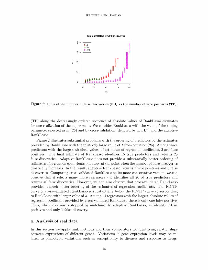
Figure 2: Plots of the number of false discoveries (FD) vs the number of true positives (TP).
(TP) along the decreasingly ordered sequence of absolute values of RankLasso estimatesfor one realization of the experiment. We consider RankLasso with the value of the tuningparameter selected as in (25) and by cross-validation (denoted by ,,cvrL”) and the adaptiveRankLasso.
Figure 2 illustrates substantial problems with the ordering of predictors by the estimatesprovided by RankLasso with the relatively large value of λ from equation (25). Among threepredictors with the largest absolute values of estimates of regression coefficiens, 2 are falsepositives. The final estimate of RankLasso identifies 15 true predictors and returns 25false discoveries. Adaptive RankLasso does not provide a substantially better ordering ofestimates of regression coefficients but stops at the point when the number of false discoveriesdrastically increases. In the result, adaptive RankLasso returns 7 true positives and 3 falsediscoveries. Comparing cross-validated RankLasso to its more conservative version, we canobserve that it selects many more regressors - it identifies all 20 of true predictors andreturns 40 false discoveries. However, we can also observe that cross-validated RankLassoprovides a much better ordering of the estimates of regression coefficients. The FD-TPcurve of cross-validated RankLasso is substantially below the FD-TP curve correspondingto RankLasso with larger value of λ. Among 14 regressors with the largest absolute values ofregression coefficient provided by cross-validated RankLasso there is only one false positive.Thus, when selection is stopped by matching the adaptive RankLasso, we identify 9 truepositives and only 1 false discovery.
4. Analysis of real data
In this section we apply rank methods and their competitors for identifying relationshipsbetween expressions of different genes. Variations in gene expression levels may be re-lated to phenotypic variations such as susceptibility to diseases and response to drugs.
18

Rank-based Lasso
Identifying the relationships between these gene expressions facilitates understanding thegenetic-pathways and identifying regulatory genes influencing the disease processes. In theconsidered data set gene expression was interrogated in lymphoblastoid cell lines of 210unrelated HapMap individuals The International HapMap Consortium (2005) from fourpopulations (60 Utah residents with ancestry from northern and western Europe, 45 HanChinese in Beijing, 45 Japanese in Tokyo, 60 Yoruba in Ibadan, Nigeria) Stranger et al.(2007). The data set can be found at ftp://ftp.sanger.ac.uk/pub/genevar/ and was pre-viously studied e.g. in Bradic et al. (2011); Fan et al. (2014). In our analysis we willconcentrate on four genes. First of them is the gene CCT8, which was analyzed previouslyin Bradic et al. (2011). This gene is within the Down syndrome critical region on humanchromosomen 21, on the minus strand. The over-expression of CCT8 may be associatedwith Down syndrome phenotypes. We also consider gene CHRNA6, which was previouslyinvestigated in Fan et al. (2014) and is thought to be related to activation of dopaminereleasing neurons with nicotine. Since the data on expression levels of these two genescontained only few relatively small outliers, we additionally considered genes PRAME andHs.444277-S, where the influence of outliers is more pronounced. The boxplots of these geneexpressions can be found in Figure 5 in the appendix.
We start with preparing the data set using three pre-processing steps as in Wang et al.(2012): we remove each probe for which the maximum expression among 210 individuals issmaller than the 25-th percentile of the entire expression values, we remove any probe forwhich the range of the expression among 210 individuals is smaller than 2 and finally weselect 300 genes, whose expressions are the most correlated to the expression level of theanalyzed gene.
Next, the data set is divided into two parts: the training set with randomly selected180 individuals and the test set with remaining 30 individuals. Five procedures from Sub-section 3 are used to select important predictors using the training set and their accuracyis evaluated using the test set. As a measure of accuracy we cannot use the standardmean square prediction error, because in the single index model (2) the link funcion g isunknown. Since the link g is increasing wrt the first variable, we can expect that the or-dering between values of the response variables Yi should be well predicted by the orderingbetween scalar products β′Xi. Moreover, from Theorem 1 we know that θ0 = γββ for thepositive multiplicative number γβ, so the ordering between Yi should be also well predictedby the ordering between (θ0)′Xi. Therefore, as a accuracy measure of estimators we use theordering prediction quality (OPQ), which is defined as follows: let T = nt(nt − 1)/2 be thenumber of different two-element subsets from the test set. The subset i, j from the testset is properly ordered, if the sign of Y test
i −Y testj coincides with the sign of θ′Xtest
i − θ′Xtestj ,
where θ is some estimator of θ0 based on the training set. Let P denote the number oftwo-element subsets from the test-set, that are properly ordered. The ordering predictionquality is defined as
OPQ =P
T. (26)
Tables 2 and 3 report the average number of selected predictors and the average valuesof OPQ over 200 random splits into the training and the test sets. These values werecalculated for all five model selection methods considered in the simulation study.
19

Rejchel and Bogdan
Table 2: Average number of selected predictors (SP)
SP rL arL rLth LADLasso cv
CCT8 16 6 6 14 25CHRNA6 19 7 7 8 52PRAME 16 6 6 6 0
Hs.444277-S 4 2 2 0 0
Table 3: Average values of the Ordering Prediction Quality (OPQ, (26))
OPQ rL arL rLth LADLasso cv
CCT8 0.74 0.73 0.74 0.73 0.76CHRNA6 0.68 0.66 0.64 0.66 0.71PRAME 0.65 0.62 0.61 0.60 0.08
Hs.444277-S 0.59 0.59 0.58 0.07 0.03
We can observe that for CCT8 the numbers of selected predictors and the predictionaccuracy of RankLasso and LADLasso are similar. The thresholded and adaptive RankLassoprovide a similar prediction accuracy with much smaller number of predictors. Interestingly,regular cross-validated Lasso yields the best Ordering Prediction Quality, which howeverrequires 4 times as many predictors as thresholded or adaptive RankLasso. For CHRNA6we see that the support of RankLasso is substantialy larger than for LADLasso and adaptiveand thresholded RankLasso, which results in slightly better prediction accuracy. Again, thebest prediction is obtained from regular cross-validated Lasso, which however uses muchlarger number of predictors.
The performance of regular Lasso drastically deteriorates for the remaining two genes,whose expressions contain substantially larger outliers. Here regular cross-validated Lassoin most of the cases is not capable of identifying any predictors. In the case of the geneHs.444277-S the same is true about LADLasso. In the case of the PRAME gene, the highestprediction accuracy is provided by regular RankLasso, which however requires almost threetimes as many predictors as adaptive or thresholded Lasso. In the case of Hs.444277-SRankLasso identifies 4 predictors, while its modified versions select only 2 genes. Thesesimple models still allow to predict the ordering of gene expressions of Hs.444277-S withaccuracy close to 60%.
5. Discussion
Lasso is a well established method for estimation of parameters in the high dimensionalregression models. It is also well understood that it can recover the support of the vector ofregression coefficients only under very stringent conditions relating the sparsity of this vectorand the structure of correlations between columns in the design matrix. This phenomenoncan be well explained using the theory of Approximate Message Algorithms (AMP), seee.g. Bayati and Montanari (2012); Su et al. (2017); Wang et al. (2017); Weinstein et al.(2020), which allows to predict the mean squared error of Lasso estimators as the functionof the tuning parameter λ. Interestingly, this error tends to take very large values for large
20

Rank-based Lasso
values of λ, which leads to early false discoveries on the Lasso path, see Su et al. (2017).Smaller values of λ typically yield smaller mean squared error and better ordering of Lassoestimates, so the estimated regression coefficients of these early false discoveries can getsmaller values than those by true discoveries. Therefore, thresholded and adaptive Lassocan recover the true model under much weaker assumptions than regular Lasso.
In this article we show that the similar phenomenon holds for RankLasso, which canbe used to identify predictors in the single-index model, with unknown monotonic linkfunction and unknown error distribution. Our theoretical and empirical results illustratethat the thresholded and adaptive versions of RankLasso can properly identify the predictorseven when the link function is non-linear, predictors are highly correlated and the errorcomes from the Cauchy distribution. When the identified model contains a small numberof predictors, the link function can be further estimated using the estimation method ofBalabdaoui et al. (2019) and its extensions based on the robust loss functions.
While our results demonstrate clearly a potential of the modified versions of RankLasso,there still remain open questions related e.g. to the choice of the optimal tuning parameterλ and the optimal threshold for the thresholded version or the optimal selection of weightsin the weighted version. In the future we plan to extend our method by exploring differentapproaches to threshold selection, including modifications of the knockoff methodology ofBarber and Candes (2015) and Candes et al. (2018). Moreover, combining the rank-basedapproach with the choice of the threshold based on the information criterion as in Bogdanet al. (2008) or Pokarowski and Mielniczuk (2015) seems also to be an interesting problemto investigate.
The theoretical analysis of RankLasso provided in this paper and the results of Kosand Bogdan (2020) on the asymptotic FDR control of the Sorted L-One Penalized Esti-mator (SLOPE, Bogdan et al. (2015)) for the regular multiple regression, pave the way forconstruction of the rank version of SLOPE, so as to obtain the asymptotic FDR controlin the single index model in the case when regressors are independent random variables.Concerning the adaptive version of RankLasso or RankSLOPE, it would be of interest todevelop an adaptive selection of weights in the spirit of Spike and Slab Lasso (Rockova andGeorge, 2018) or the adaptive Bayesian version of SLOPE (Jiang et al., 2019).
Finally, a single index model (2), which is studied in the paper, can be generalized to
Yi = g(β′1Xi, . . . , β′dXi, εi),
where β1, β2, . . . , βd are p-dimensional vectors and d < p. Such model was studied, for in-stance, in Cohen et al. (2012). The question arises whether the rank-based approach canproperly identify true predictors also for the case d > 1. A similar problem in the context ofmisspecified binary regression was considered in Kubkowski and Mielniczuk (2018), whereit is shown that the vector of parameters estimated by logistic regression can be expressedas a linear combination of vectors β1, . . . , βd under a natural extension of our Assumption2. The analysis from Kubkowski and Mielniczuk (2018) seems to be a good starting pointin establishing a similar relation for our parameter θ0 given in (7). If this holds, thenthe theoretical results concerned with the identification of significant predictors by Ran-kLasso should be possible to obtain by a relatively straightforward extension of our prooftechniques.
21

Rejchel and Bogdan
Acknowledgments
We would like to thank Patrick Tardivel for helpful comments. We gratefully acknowledgethe grant of the Wroclaw Center of Networking and Supercomputing (WCSS), where mostof the computations were performed. Ma lgorzata Bogdan is supported by Polish NationalScience Center grants no. 2016/23/B/ST1/00454. We would like also to thank the AssociateEditor and two reviewers for their comments, which helped us improve the manuscript.
Appendix
In Section A of the appendix we provide results for Rank-Lasso and its modifications inthe low-dimensional scenario. Besides, additional results of numerical experiments are inSection E. The proofs of results obtained in the main paper are given in Sections B and C.Finally, proofs of results from Section A in the appendix are given in Section D.
Appendix A. Low-dimensional scenario
In this section we consider properties of rank estimators in the case where the number ofpredictors is fixed. In the first part we focus on RankLasso and in the second part we studythresholded and weighted RankLasso.
We assume, without loss of generality, that T = 1, . . . , p0 for some 0 < p0 < p, so theresponse variable Y depends on first p0 predictors. RankLasso estimates the set T by
T = 1 ≤ j ≤ p : θj 6= 0.
The results, that we obtain in this subsection, are asymptotic, so we can replace thetrue parameter θ0 in (10) by
θ∗ =n
n− 1θ0 = H−1µ. (27)
Obviously, it does not change the set of relevant predictors T. We also decompose the matrixH = EX1X
′1 as
H =
p0×p0︷︸︸︷H1
p0×(p−p0)︷︸︸︷H2
H ′2 H3
,
so the matrix H1 describes correlations between relevant predictors and the matrix H2
contains correlations between relevant and irrelevant predictors.
A.0.1 Model selection consistency of RankLasso
The next result provides sufficient and necessary conditions for RankLasso to be modelselection consistent. They are similar to the results proved in Zou (2006, Theorem 1)and Zhao and Yu (2006, Theorem 1), which concern model selection in the linear model.Theorem 8 extends these results to the single index model (2), which does not require anyassumptions on the form of the link function (except being monotonic) nor the distributionof the noise variable.
22

Rank-based Lasso
Theorem 8 Suppose that Assumption 3 is satisfied, E|X1|4 <∞ and λ→ 0,√nλ→∞.
(a) If limn→∞ P (T = T )→ 1, then∣∣H ′2H−11 sign(θ∗T )
∣∣∞ ≤ 1, (28)
where θ∗ is defined in (27).(b) If the inequality ∣∣H ′2H−1
1 sign(θ∗T )∣∣∞ < 1 (29)
holds, then limn→∞ P (T = T )→ 1.
The sufficiency of (29) for model selection consistency of RankLasso was established inWang and Zhu (2015, Corollary 2.1). In Theorem 8 we strenghten this result by showing thatit is almost the necessary condition. The condition (29), called the irrepresentable condition(Zhao and Yu, 2006), is restrictive and satisfied only in some very special cases, like whenpredictors are independent or when the correlations between ,,neighboring” variables decayexponentially with their distance. Therefore, RankLasso usually is not consistent in modelselection. However, as shown in the following Lemma 9, it can consistently estimate θ∗
under much weaker assumptions. This result will be crucial for Subsection A.0.2, where weestablish model selection consistency of the thresholded and weighted versions of RankLassounder such weaker assumptions. The next fact is a generalization of Knight and Fu (2000,Theorem 2).
Lemma 9 Suppose that Assumption 1 is satisfied and E|X1|4 < ∞. Let an be a sequencesuch that an → 0, 1
an√n→ b ∈ [0,∞), λ
an→ c ∈ [0,∞). Then the RankLasso estimator θ
in (5) satisfies1
an
(θ − θ∗
)→d arg min
θV (θ),
where
V (θ) =1
2θ′Hθ + b θ′W + c
∑j∈T
θjsign(θ∗j ) + c∑j /∈T
|θj |
and W has a normal N(0, D) distribution with the matrix D given in Lemma 17 in Sec-tion D.
A.0.2 Modifications of RankLasso
In this subsection we introduce two modifications of RankLasso and study their propertiesin the low-dimensional case.
First of these modifications, the weighted RankLasso estimator, is an analogue of theadaptive Lasso, which was proposed in Zou (2006). The main idea of this approach relieson the application of different weights for different predictors, depending on the value ofsome initial estimator θ of θ∗. This estimator needs to be
√n-consistent, i.e. it satisfies
√n(θ − θ∗
)= OP (1) . (30)
23

Rejchel and Bogdan
In particular, according to Lemma 9, θ can be chosen as the RankLasso estimator withthe regularization parameter that behaves as O(1/
√n). Then, the weighted RankLasso
estimator θa is obtained as
θa = arg minθ∈Rp
Q(θ) + λ
p∑j=1
wj |θj | , (31)
where wj = |θj |−1, j = 1, . . . , p and Q(θ) is given in (6).
Let T a denote a set j ∈ 1, . . . , p : θaj 6= 0. The properties of θa are described in thenext theorem.
Theorem 10 Consider the weighted RankLasso estimator (31) with θ satisfying (30). Sup-pose that Assumption 3 is satisfied and E|X1|4 < ∞. If nλ → ∞ and
√nλ → c ∈ [0,∞),
then(a) lim
n→∞P(
sign(θa) = sign(β))
= 1, where the equality of signs of two vectors is understood
componentwise,
(b)√n(θaT − θ∗T
)→d N
(−H−1
1 c, H−11 D1H
−11
), where c = c
(1θ∗1, . . . , 1
θ∗p0
), θ∗ is defined
in (27) and the matrix D1 is the (p0 × p0) upper-left submatrix of the matrix D defined inLemma 17 in Section D.
Now, we introduce the second modification, which is thresholded RankLasso. Thisestimator is denoted by θth and defined in (19).
Theorem 11 Suppose that Assumption 3 is satisfied and E|X1|4 <∞. If√nλ→ 0, δ → 0
and√nδ →∞, then
(a) limn→∞
P(
sign(θth) = sign(β))
= 1, where the equality of signs of two vectors is understood
componentwise,
(b)√n(θthT − θ∗T
)→d N
(0,(H−1DH−1
)1
), where θ∗ is defined in (27) and
(H−1DH−1
)1
is the (p0 × p0) upper-left submatrix of H−1DH−1.
Theorems 10 and 11 state that weighted and thresholded RankLasso behave almost likethe oracle. They are asymptotically able to identify the support and recognize the signsof coordinates of the true parameter β. Moreover, they estimate nonzero coordinates ofθ∗ with the standard
√n-rate. The crucial fact is that these theorems hold even when the
irrepresentable condition is not satisfied. Thus, both modifications of RankLasso allow toidentify the true model under much weaker assumptions than vanilla RankLasso.
Theorems 10 and 11 work in the single index model (2) and they do not require anyassumptions on the distribution of the noise variables or the form of the increasing linkfunction g. Comparing to other theoretical results concerning model selection with therobust loss functions, like Wang et al. (2007, Theorem) , Johnson and Peng (2008, Theorem2.1), Song and Ma (2010, Theorem 4.2), Rejchel (2017b, Theorem 4.1), Avella-Medina andRonchetti (2018, Theorem 2), the assumptions of Theorems 10 and 11 are slightly stronger.Specifically, in Theorems 10 and 11 the standard condition on the existence of the secondmoment of predictors is replaced by the assumption on the existence of the fourth moment.
24

Rank-based Lasso
This results from the fact that we work with the nonlinear model and the quadratic lossfunction. Apart from computational efficiency, application of the quadratic loss functionallows us to solve the theoretical issues related to the dependency between ranks. Thestronger assumption on the moments of predictors seems to be a relatively small prize forthe gain in computational complexity, which allows to handle large data sets. Moreover,according to the simulation study reported in Section 3 of the main paper, for such largedata sets our method has substantially better statistical properties than LADLasso, whichis a popular methodology for robust model selection.
Appendix B. Results from Subsection 2.2
Notice that for Q(θ) defined in (6) we have
Q(θ) =1
2n
n∑i=1
(Ri/n− θ′Xi
)2+ θ′X/2− n+ 1
4n+ 1/8.
Therefore, due to the fact that predictors Xi are centred we will consider Q(θ) withoutsubtracting 0.5, that is
Q(θ) =1
2n
n∑i=1
(Ri/n− θ′Xi
)2in all proofs in this appendix. It will simplify notations.Proof [Proof of Theorem 1] We start with proving the first part of the theorem. Argumenta-tion is similar to the proof of Li and Duan (1989, Theorem 2.1), but it has to be adjusted toranks, which are not independent random variables (as distinct from Y1, . . . , Yn). Obviously,we have
EQ(θ) =1
2n3
n∑i=1
ER2i −
1
n2
n∑i=1
ERiθ′Xi +1
2n
n∑i=1
E(θ′Xi
)2.
Vectors (X1, Y1), . . . , (Xn, Yn) are i.i.d. and Xi are centred, so for all i 6= 1
ERiθ′Xi = EI(Y1 ≤ Yi)θ′Xi +∑
j 6=1,i
EI(Yj ≤ Yi)θ′Xi
= EI(Yi ≤ Y1)θ′X1 +∑
j 6=1,i
EI(Yj ≤ Y1)θ′X1 = ER1θ′X1.
Moreover, ranks R1, . . . , Rn have the same distribution, so∑n
i=1 ER2i = nER2
1. Therefore,
we obtain that EQ(θ) = 12E(R1n − θ
′X1
)2. Using Jensen’s inequality and Assumption 2 we
have
EQ(θ) =1
2EE
[(R1
n− θ′X1
)2
|β′Xi, εi, i = 1, . . . , n
]
≥ 1
2E[E(R1
n− θ′X1|β′Xi, εi, i = 1, . . . , n
)]2
=1
2E[R1
n− E
(θ′X1|β′X1
)]2
=1
2E(R1
n− dθβ′X1
)2
≥ mind∈R
EQ(dβ).
25

Rejchel and Bogdan
Obviously, we have mind EQ(dβ) = EQ(γββ), where γβ is defined in (12). Since θ0 is theunique minimizer of EQ(θ), we obtain the first part of the theorem.
Next, we establish the second part of the theorem. Denote Z = β′X1 and ε = ε1. It isclear that γβ > 0 is equivalent to Cov(Z,F (g(Z, ε))) > 0. This covariance can be expressedas
EZF (g(Z, ε)) = Eh(ε), (32)
where h(a) = E [ZF (g(Z, ε))|ε = a] = EZF (g(Z, a)) for arbitrary a. This fact simply fol-lows from EZ = 0 and independence between Z and ε. If F is increasing and g is increasingwith respect to the first variable, then h(a) > 0 for arbitrary a by Lemma 12 given below.Obviously, it implies that (32) is positive.
The following result was used in the proof of Theorem 1. It is a simple and convenientadaptation of a well-known fact concerning covariance of nondecreasing functions (Thoris-son, 1995). Its proof follows Kubkowski (2019, Lemma A.44).
Lemma 12 Let U be a random variable that is not concentrated at one point, i.e. P (U =u) < 1 for each u ∈ R. Moreover, let f, h : R → R be increasing functions. ThenCov(f(U), h(U)) > 0.
Proof For all real a 6= b we have [f(a)− f(b)][h(a)−h(b)] > 0, because f, h are increasing.Let V be an independent copy of U. Then P (U 6= V ) > 0 and we obtain
0 < E[f(U)− f(V )][h(U)− h(V )] I(U 6= V )
= E[f(U)− f(V )][h(U)− h(V )]
= 2Ef(U)h(U)− 2Ef(U)Eh(U)
= 2Cov(f(U), h(U)).
Appendix C. Results from Subsection 2.3
To prove Theorem 2 we need three auxiliary results: Lemma 13, Lemma 14 and Lemma15. The first one is borrowed from van de Geer (2016, Corollary 8.2), while the second oneis its adaptation to U -statistics.
Lemma 13 Suppose that Z1, . . . , Zn are i.i.d. random variables and there exists L > 0such that C2 = E exp (|Z1|/L) is finite. Then for arbitrary u > 0
P
(1
n
n∑i=1
(Zi − EZi) > 2L
(C
√2u
n+u
n
))≤ exp(−u).
Lemma 14 Consider a U -statistic
U =1
n(n− 1)
∑i 6=j
h(Zi, Zj)
26

Rank-based Lasso
with a kernel h based on i.i.d. random variables Z1, . . . , Zn. Suppose that there exists L > 0such that C2 = E exp (|h(Z1, Z2)|/L) is finite. Then for arbitrary u > 0
P
(U − EU > 2L
(C
√6u
n+
3u
n
))≤ exp(−u).
Proof Let g(z1, z2) = h(z1, z2)−Eh(Z1, Z2) and U be a U -statistic with a kernel g. UsingHoeffding’s decomposition we can represent every U -statistic as an average of (dependent)averages of independent random variables (Serfling, 1980), i.e.
U =1
n!
∑π
1
N
N∑i=1
g(Zπ(i), Zπ(N+i)
), (33)
whereN =⌊n2
⌋and the first sum on the right-hand side of (33) is taken over all permutations
π of a set 1, . . . , n. Take arbitrary s > 0. Then using Jensen’s inequality and the fact thatZ1, . . . , Zn are i.i.d. we obtain
E exp(sU) ≤ 1
n!
∑π
E exp
[s
N
N∑i=1
g(Zπ(i), Zπ(N+i)
)]
= E exp
[s
N
N∑i=1
g (Zi, ZN+i)
]. (34)
We have the average of N -i.i.d. random variables in (34), so we can repeat argumentationfrom the proof of van de Geer (2016, Corollary 8.2). Finally, we use the simple inequalityN ≥ n/3 for n ≥ 2.
Lemma 15 Suppose Assumptions 3 and 4 are satisfied. For arbitrary j = 1, . . . , p andu > 0 we have
P
(1
n
n∑i=1
XijX′iθ
0 − n− 1
nµj > 5
τ2
√κ
(2
√2u
n+u
n
))≤ exp(−u). (35)
Besides, if X1 has a normal distribution N(0, H), then we can drop τ and κ in (35).
Proof Fix j = 1, . . . , p and u > 0. Recall that Hθ0 = n−1n µ by (10). We work with an
average of i.i.d. random variables, so we can use Lemma 13. We only have to find L,C > 0such that
E exp(|X1jX
′1θ
0|/L)≤ C2.
For each positive number a, b, s we have the inequality ab ≤ a2
2s2+ b2s2
2 . Applying this factand the Schwarz inequality we obtain
E exp(|X1jX
′1θ
0|/L)≤
√√√√E exp
(X2
1j
s2L
)E exp
(s2(X ′1θ
0)2
L
)(36)
27

Rejchel and Bogdan
and the number s will be chosen later. The variable X1j is subgaussian, so using Baraniuk
et al. (2011, Lemma 7.4) we can bound the first expectation in (36) by(
1− 2τ2
s2L
)−1/2pro-
vided that s2L > 2τ2. The second expectation in (36) can be bounded using subgaussianityof the vector X1 in the following way
E exp
(s2(X ′1θ
0)2
L
)≤(
1− 2s2τ2|θ0|22L
)−1/2
,
provided that 2s2τ2|θ0|22 < L. From Theorem 1 we obtain two equalities θ0 = γββ and
γβ =n−1n
E I(Y2≤Y1)β′X1
β′Hβ . Recall that κ is the smallest eigenvalue of the matrix HT . Therefore,we obtain a bound
|θ0|22 = γ2β|βT |22 ≤ κ−1,
because
E I(Y2 ≤ Y1)β′X1 ≤√β′THTβT .
Taking L = 2.2τ2/√κ and s2 =
√κ we obtain C ≤ 2, that finishes the proof of the first
part of the lemma.Next, we assume thatX1 ∼ N(0, H). Therefore, X1j ∼ N(0, 1) and (θ0)′X1 ∼ N(0, (θ0)′Hθ0).
The argumentation is as above with s2 = 1. We only use the inequality (θ0)′Hθ0 ≤ 1 andthe equality
E exp((X ′1θ
0)2/L)
=(1− 2(θ0)′Hθ0/L
)−1/2,
provided that L > 2(θ0)′Hθ0. Therefore, we can take L = 2.2.
Lemma 16 Suppose that Assumption 4 and (14) are satisfied. Then for arbitrary a ∈(0, 1), q ≥ 1, ξ > 1 with probability at least 1− 2a we have Fq(ξ) ≥ Fq(ξ)/2.
ProofFix a ∈ (0, 1), q ≥ 1, ξ > 1. We start with considering the l∞-norm of the matrix∣∣∣∣ 1nX ′X −H
∣∣∣∣∞
= maxj,k=1,...,p
∣∣∣∣∣ 1nn∑i=1
XijXik − EX1jX1k
∣∣∣∣∣ .Fix j, k ∈ 1, . . . , p. Using subgaussianity of predictors, Lemma 13 and argumentationsimilar to the proof of Lemma 15 we have for u = log(p2/a)
P
(∣∣∣∣∣ 1nn∑i=1
XijXik − EX1jX1k
∣∣∣∣∣ > K2τ2
√log(p2/a)
n
)≤ 2a
p2,
where K2 is an universal constant.Therefore, using union bounds we obtain
P
(∣∣∣∣ 1nX ′X −H∣∣∣∣∞> K2τ
2
√log(p2/a)
n
)≤ 2a. (37)
28

Rank-based Lasso
Obviously, we have |(X ′X/n−H)θ|∞ ≤ |X ′X/n−H|∞|θ|1 and for each θ ∈ C(ξ) and q > 1
we obtain |θ|1 ≤ (1 + ξ)|θT |1 ≤ (1 + ξ)p1−1/q0 |θT |q ≤ (1 + ξ)p
1−1/q0 |θ|q. Therefore, for each
θ ∈ C(ξ)
p1/q0 |X ′Xθ/n|∞
|θ|q≥ p
1/q0 |Hθ|∞|θ|q
− p1/q0 |X ′X/n−H|∞|θ|1
|θ|q
≥ p1/q0 |Hθ|∞|θ|q
− (1 + ξ)p0|X ′X/n−H|∞.
Taking infimum and using (37), we have the following probabilistic inequality
Fq(ξ) ≥ Fq(ξ)−K2(1 + ξ)p0τ2
√log(p2/a)
n.
To finish the proof we use (14) with K1 being sufficiently large.
Proof [Proof of Theorem 2]
Let a ∈ (0, 1) be arbitrary. The main part of the proof is to show that with highprobability
|θ − θ0|q ≤2ξp
1/q0 λ
(ξ + 1)Fq(ξ). (38)
Then we apply Lemma 16 to obtain (16).
Thus, we focus on proving (38). Denote Ω = |∇Q(θ0)|∞ ≤ ξ−1ξ+1λ. We start with lower
bounding probability of Ω. For A defined in (11) and every j = 1, . . . , p we obtain
∇jQ(θ0) =
[1
n
n∑i=1
XijX′iθ
0 − n− 1
nµj
]+n− 1
n
[µj −Aj
]− 1
n2
n∑i=1
Xij , (39)
so if we find probabilistic bounds for each term on the right-hand side of (39), then usingunion bounds we get the bound for |∇Q(θ0)|∞. Consider the middle term in (39). By (24)we apply Lemma 14 with h(z1, z2) = 1
2 [I(y2 ≤ y1)x1j + I(y1 ≤ y2)x2j ] . Variables X1j andX2j are i.i.d., so for arbitrary L > 0 we have
E exp (|h(Z1, Z2|/L) ≤ [E exp (|X1j |/(2L))]2 . (40)
Using the fact that the variable X1j is subgaussian we bound (40) by 4 exp(τ2
4L2
). Taking
L = τ and u = log(p/a) in Lemma 14 we obtain for some universal constant K1
P
(Aj − µj > K1τ
√log(p/a)
n
)≤ a
p.
The third term in (39) can be handled similarly using Lemma 13. To obtain the boundfor the first term in (39) we apply Lemma 15. Taking these results together and using unionbounds we obtain that P (Ω) ≥ 1−K2a provided that λ satisfies (15).
29

Rejchel and Bogdan
In further argumentation we consider only the event Ω. Besides, we denote θ = θ − θ0,where θ is a minimizer of a convex function (5), that is equivalent to
∇jQ(θ) = −λsign(θj) for θj 6= 0,
|∇jQ(θ)| ≤ λ for θj = 0,(41)
where j = 1, . . . , p.First, we prove that θ ∈ C(ξ). Here our argumentation is standard (Ye and Zhang, 2010).
From (41) and the fact that |θ|1 = |θT |1 + |θT ′ |1 we can calculate
0 ≤ θ′X ′Xθ/n = θ′[∇Q(θ)−∇Q(θ0)
]=∑j∈T
θj∇jQ(θ) +∑j∈T ′
θj∇jQ(θ)− θ′∇Q(θ0)
≤ λ∑j∈T|θj | − λ
∑j∈T ′|θj |+ |θ|1|∇Q(θ0)|∞
=[λ+ |∇Q(θ0)|∞
]|θT |1 +
[|∇Q(θ0)|∞ − λ
]|θT ′ |1 .
Thus, using the fact that we consider the event Ω we get
|θT ′ |1 ≤λ+ |∇Q(θ0)|∞λ− |∇Q(θ0)|∞
|θT |1 ≤ ξ|θT |1 .
Therefore, from the definition of Fq(ξ) we have
|θ − θ0|q ≤p
1/q0 |X ′X(θ − θ0)/n|∞
Fq(ξ)≤ p1/q
0
|∇Q(θ)|∞ + |∇Q(θ0)|∞Fq(ξ)
.
Using (41) and the fact, that we are on Ω, we obtain (38).The case X1 ∼ N(0, H) is a consequence of the analogous part of Lemma 15.
Proof [Proof of Corollary 3] The proof is a simple consequence of the bound (16) withq =∞ obtained in Theorem 2. Indeed, for arbitrary predictors j ∈ T and k /∈ T we obtain
|θj | ≥ |θ0j | − |θj − θ0
j | ≥ θ0min − |θ − θ0|∞ >
4ξλ
(ξ + 1)F∞(ξ)≥ |θk − θ0
k| = |θk|.
Proof [Proof of Theorem 5] The proof is a simple consequence of the uniform bound (18)from Corollary 4. Indeed, for an arbitrary j /∈ T we obtain
|θj | = |θj − θ0j | ≤ K4λ < δ ,
so j /∈ T th. Analogously, if j ∈ T, then
|θj | ≥ |θ0j | − |θj − θ0
j | ≥ 2δ −K4λ > δ .
30

Rank-based Lasso
Proof [Proof of Theorem 7] First, we define a function
Γa(θ) = Q(θ) + λa
p∑j=1
wj |θj |. (42)
Next, we fix a ∈ (0, 1) and set, for simplicity, ξ0 = 3. Consider the event Ω = |∇Q(θ0)|∞ ≤λ/2. We know from the proof of Theorem 2 that P (Ω) ≥ 1−K3a and the inequality (18)is satisfied. The proof of Theorem 7 consists of two steps. In the first one we show thatwith high probability there exists a minimizer of the function
g(θT ) = Γa(θT , 0)
that is close to θ0T in the l1 norm. We denote this minimizer by θaT . In the second part of the
proof we obtain that the vector (θaT , 0), that is θaT augmented by (p− p0) zeros, minimizesthe function (42).
First, consider vectors v ∈ Rp0 having a fixed common l1-norm and a sphere
θT = θ0T + p0λv. (43)
Suppose that |v|1 is sufficiently large. We take arbitrary θT from the sphere (43) andcalculate that
Q(θT , 0)−Q(θ0) =1
2p2
0λ2v′
1
nX ′TXT v + p0λv
′[∇Q(θ0)]T .
Let κ be the minimal eigenvalue of the matrix 1nX′TXT . Then we have v′ 1nX
′TXT v ≥
κ|v|21/p0. Besides, on the event Ω we obtain
|v′[∇Q(θ0)]T | ≤ |v|1|[∇Q(θ0)]T |∞ ≤ λ|v|1/2.
Proceeding analogously to the proof of Lemma 16 we can show that κ ≥ κ/2 with probabilityclose to one. Therefore, we obtain
Q(θT , 0)−Q(θ0) ≥ κp0λ2|v|21/4− p0λ
2|v|1/2. (44)
Next, we work with the penalty term and obtain∣∣∣∣∣∣λap0∑j=1
wj[|θ0j + p0λvj | − |θ0
j |]∣∣∣∣∣∣ ≤ λap0λ
p0∑j=1
wj |vj |. (45)
Moreover, for j ∈ T we have from Corollary 4 that
|θj | ≥ |θ0j | − |θj − θ0
j | ≥ θ0min −K4λ > λa,
so wj ≤ K. Therefore, the right-hand side of(45) is bounded by Kλλap0|v|1. Combining itwith (44) we get
g(θT )− g(θ0T ) ≥ p0λ
2|v|1 (κ|v|1/4− 1/2−K4K) . (46)
31

Rejchel and Bogdan
The right-hand side of (46) is positive, because the norm |v|1 can be taken sufficiently large,K,K4 are constants and κ is lower bounded by a constant. Therefore, the convex functiong(θT ) takes on a sphere (43) values larger than in the center θ0
T . So, there exists a minimizerinside this sphere.
Next, we show that the random vector (θaT , 0) minimizes (42) with high probability, sowe have to prove that the event
|∇jQ(θaT , 0)| ≤ wjλa for every j /∈ T (47)
has probability close to one. By Corollary 4 we have for j /∈ T
|θj | = |θj − θ0j | ≤ K4λ.
Therefore, the corresponding weight wj ≥ λ−1a . We can also calculate that
∇Q(θT , 0) =1
nX ′XT θT −
[n− 1
nA+
1
n2
n∑i=1
Xi
],
so we obtain the inequality
∣∣∣[∇Q(θaT , 0)]T ′
∣∣∣∞≤∣∣∣∣ 1nX ′T ′XT (θaT − θ0
T )
∣∣∣∣∞
+∣∣[∇Q(θ0)
]T ′
∣∣∞ . (48)
Consider the event Ω = |∇Q(θ0)|∞ ≤ λ/2 that has probability close to one by the proofof Theorem 2. Then the second term on the right-hand side of (48) can be bounded by λ/2.The former one can be decomposed as∣∣∣∣ 1nX ′T ′XT (θaT − θ0
T )
∣∣∣∣∞≤
∣∣∣∣( 1
nX ′T ′XT −H ′2
)(θaT − θ0
T )
∣∣∣∣∞
+∣∣∣H ′2(θaT − θ0
T )∣∣∣∞
≤∣∣∣∣ 1nX ′T ′XT −H ′2
∣∣∣∣∞
∣∣∣θaT − θ0T
∣∣∣1
+∣∣H ′2∣∣∞ ∣∣∣θaT − θ0
T
∣∣∣1. (49)
The expression |H2|∞ is bounded by one, so from the first part of the proof we can bound,with high probability, the second term in (49) by K6p0λ. The l∞-norm in the former ex-
pression can be bounded, with probability close to one, by K7
√log(p/a)
n as in the proof ofLemma 16. Therefore, we have just proven that with probability close to one∣∣∣[∇Q(θaT , 0)
]T ′
∣∣∣∞≤ K8p0λ.
Combining it with the fact that wj ≥ λ−1a we obtain that the event (47) has probability
close to one, because from assumptions of the theorem p0λ ≤ K5 for K5 small enough.
32

Rank-based Lasso
Appendix D. Results from Section A
We start with the proof of Lemma 9. Then we state Lemma 17 that is also needed in proofsof Theorems 8, 10 and 11. We will use the following notation
Γ(θ) = Q(θ) + λ|θ|1. (50)
Proof [Proof of Lemma 9] Let a := an be a fixed sequence such that a → 0. We cancalculate that for every θ
Q(θ∗ + aθ)−Q(θ∗) = − a
n2θ′
(n∑i=1
RiXi
)+ aθ′
(X ′X
n
)θ∗ +
a2
2θ′(X ′X
n
)θ. (51)
Using (9) we obtain that the right-hand side of (51) is
a2
2θ′(X ′X
n
)θ − aθ′
[n− 1
nA+ X/n−
(X ′X
n
)θ∗],
where A is defined in (11). Therefore, we have
1
a2[Q(θ∗ + aθ)−Q(θ∗)] =
1
2θ′(X ′X
n
)θ
− θ′√na
[n− 1
n
√nA+ X/
√n−
(X ′X√n
)θ∗].
Using LLN, Lemma 17 (given below) and Slutsky’s theorem we get that
1
a2[Q(θ∗ + aθ)−Q(θ∗)]→f−d
1
2θTHθ + bθ′W, (52)
where →f−d is the finite-dimensional convergence in distribution and W ∼ N(0, D). Next,we consider the penalty term and notice that
λ
a2
p∑j=1
(|θ∗j + aθj | −
∣∣θ∗j ∣∣)→ c∑j∈T
θjsign(θ∗j ) + c∑j /∈T
|θj |. (53)
Thus, from (52) and (53) we have the convergence of convex functions
1
a2[Γ(θ∗ + aθ)− Γ(θ∗)]→f−d V (θ), (54)
where the function Γ(θ) is defined in (50). The function on the left-hand side of (54) is min-
imized by 1a
(θ − θ∗
)and the convex function on the right-hand side of (54) has a unique
minimizer. Thus 1a
(θ − θ∗
)→d arg min
θV (θ), see Geyer (1996).
Lemma 17 Suppose that Assumption 1 is satisfied and E|X1|4 <∞. Then
√n [A− µ]−
√n
[X ′X
nθ∗ − µ
]→d N(0, D),
where D is stated precisely in the proof below.
33

Rejchel and Bogdan
Proof Consider two U -statistics. The first one is A that is defined in (11). The secondU -statistic is
B =1
n
n∑i=1
XiX′iθ∗
and is of the order one. Besides, we have EB = Hθ∗ = µ by (27). Using Hoeffding (1948,Theorem 7.1) we obtain convergence in distribution in R2p
√n
[A− µB − µ
]→d N(0,Σ)
for the matrix
Σ =
p×p︷︸︸︷Σ1
p×p︷︸︸︷Σ2
Σ2 Σ3
,
where for j, k = 1, . . . , p and the function f in (24) we have
(Σ1)jk = 4Cov(fj(Z1), fk(Z1)),
where f(z1) = E [f(Z1, Z2)|Z1 = z1] and fj(z1) is its j-th coordinate. The entries of thematrix Σ3 are
(Σ3)jk = Cov(X1jX′1θ∗, X1kX
′1θ∗)
and
(Σ2)jk = 2Cov(fj(Z1), X1kX′1θ∗).
Next, define (p × 2p)-dimensional matrix M in the following way: for j = 1, . . . , p putMj,j = 1 and Mj,p+j = −1, and zeros elsewhere. Then
√n [A− µ]−
√n
[X ′X
nθ∗ − µ
]= M
√n
[A− µB − µ
]→d N(0,MΣM ′).
Now we prove main results of Section A.
Proof [Proof of Theorem 8] From Lemma 9 for a = λ we obtain
λ−1(θ − θ∗
)→d arg min
θV2(θ), (55)
where
V2(θ) =1
2θ′Hθ +
∑j∈T
θjsign(θ∗j ) +∑j /∈T
|θj |. (56)
We start with the case (b). Let η = arg minθ V2(θ). We know that η is nonrandom and thefunction V2(θ) is strictly convex. Therefore, using (29) we have
η =(−H−1
1 sign(θ∗T ), 0). (57)
34

Rank-based Lasso
For fixed j ∈ T we have
λ−1(θj − θ∗j
)→P ηj ,
so P(j /∈ T ) = P(θj = 0) → 0. Thus, P(T ⊂ T ) → 1. Next, we show that P(T ⊂ T ) ≥1−
∑j /∈T
P(j ∈ T )→ 1. Consider fixed j /∈ T and an event j ∈ T. Recall that θ minimizes
the convex function Γ, so 0 ∈ ∂Γ(θ), where ∂Γ denotes a subgradient of the convex functionΓ. The function Q(θ) is differentiable, so ∂Γ(θ) = ∇Q(θ) + λ∂|θ|. Therefore, we have
0 = ∇jQ(θ) + λ sign(θj), (58)
where ∇jQ(θ) is the j-th partial derivative Q(θ) at θ. From (58) we have
λ−1∣∣∣∇jQ(θ)
∣∣∣ = 1. (59)
We can calculate that
∇Q(θ) = −n− 1
nA− X/n+
X ′X
n
(θ − θ∗
)+X ′X
nθ∗,
that gives us
λ−1∇Q(θ) = − 1√nλ
[n− 1
n
√nA+ X/
√n−√nX ′X
nθ∗]
+ λ−1X′X
n(θ − θ∗). (60)
Therefore, using LLN, Lemma 17, (55) and Slutsky’s theorem the left-hand side of (59)
tends in probability to∣∣∣(Hη)j
∣∣∣ . Recall that we consider the event j ∈ T for j /∈ T, so we
have the inequality
lim supn→∞
P(θj 6= 0
)≤ I
(∣∣∣(Hη)j
∣∣∣ = 1),
since η is not random. However, from (29) and (57) we obtain∣∣∣(Hη)j
∣∣∣ =∣∣∣(HT
2 H−11 sign (θ∗A)
)j
∣∣∣ < 1.
Therefore, probability P(θj 6= 0
)tends to zero that finishes the proof of consistency in
model selection.The proof of the claim (a) is similar to the proof of Zou (2006, Theorem 1, scenario
(3)) and uses properties of the function V2(θ) in (56). We state it here for completenessof the paper. For each j /∈ T we have λ−1θj →p ηj , so using model selection consistency
of the estimator θ we obtain ηT ′ = 0. Moreover, the function V2(θ) is convex and η is itsminimizer, so 0 ∈ ∂V2(η). Thus, if j ∈ T we have 0 = (Hη)j + sign(θ∗j ). Therefore, we get
ηT = −H−11 sign(θ∗T ), (61)
because ηT ′ = 0. While for j /∈ T we obtain that |(Hη)j | ≤ 1, so component-wise
|H ′2ηT | ≤ 1. (62)
35

Rejchel and Bogdan
Claim (a) follows from combination of (61) and (62).
In the next result we use epi-convergence in distribution, which is an useful tool in theoptimization theory. The following definitions are borrowed from Geyer (1994) and Pflug(1995).
Definition 1 (Epi-convergence) A sequence fn of lower semicontinuous (lsc) functionsfrom Rp to R epi-converges to a lsc function f, if for all x and xn → x the following inequalityholds lim infn fn(xn) ≥ f(x) and there exists xn → x such that lim supn fn(xn) ≤ f(x).
Definition 1 is equivalent to the following one, which is useful to define epi-convergencein distribution.
Definition 2 (Epi-convergence) A sequence fn of lower semicontinuous (lsc) functionsfrom Rp to R epi-converges to a lsc function f, if for each compact set K the follow-ing inequality holds lim infn infx∈K fn(x) ≥ infx∈K f(x) and for each open set O we havelim supn infx∈O fn(x) ≤ infx∈O f(x).
Definition 3 (Epi-convergence in distribution) Let Zn and Z be random processes,which are lsc on Rp. We say that Zn epi-converges in distribution to Z, if for all k, allclosed rectangles R1, . . . , Rk with open interiors Ro1, . . . , R
ok and any real numbers a1, . . . , ak
we have
P
(infu∈R1
Z(u) > a1, . . . , infu∈Rk
Z(u) > ak
)≤ lim inf
nP
(infu∈R1
Zn(u) > a1, . . . , infu∈Rk
Zn(u) > ak
)≤ lim sup
nP
(infu∈Ro
1
Zn(u) ≥ a1, . . . , infu∈Ro
k
Zn(u) ≥ ak)
≤ P
(infu∈Ro
1
Z(u) ≥ a1, . . . , infu∈Ro
k
Z(u) ≥ ak).
Proof [Proof of Theorem 10] We define a function
Γa(θ) = Q(θ) + λ
p∑j=1
|θj ||θj |
.
Let us start with the claim (b). Repeating the same arguments as in the proof of Lemma 9(for a = 1√
n) we obtain for every θ
nQ
(θ∗ +
θ√n
)− nQ(θ∗)→f−d
1
2θ′Hθ + θ′W,
which using convexity implies weak convergence of the stochastic processnQ
(θ∗ +
θ√n
)− nQ(θ∗) : θ ∈ K
→d
1
2θ′Hθ + θ′W : θ ∈ K
(63)
36

Rank-based Lasso
for every compact set K in Rp, see Arcones (1998). Now consider the penalty term and usesimilar arguments to that in the proof of Zou (2006, Theorem 2) to obtain that if θ∗j 6= 0,then
nλ
∣∣∣θ∗j +
θj√n
∣∣∣− |θ∗j ||θj |
=√nλ√n
∣∣∣θ∗j +
θj√n
∣∣∣− |θ∗j ||θj |
→P cθjθ∗j,
because√nλ → c, θj →P θ∗j and
√n[∣∣∣θ∗j +
θj√n
∣∣∣− |θ∗j |] → sign(θ∗j )θj . However, if θ∗j = 0,
then
nλ
∣∣∣θ∗j +
θj√n
∣∣∣− |θ∗j ||θj |
=√nλ|θj ||θj |→P
0, θj = 0∞, θj 6= 0,
since√nθj = OP (1) and nλ→∞. Therefore, we obtain that for every θ
nλ
p∑j=1
∣∣∣θ∗j +θj√n
∣∣∣− |θ∗j ||θj |
→P
c∑
j∈Tθjθ∗j, θ = (θ1, . . . , θp0 , 0, . . . , 0)
∞, otherwise.
Since we have infinity in the last limit we cannot use arguments based on uniform con-vergence on compacts as we have done in the proof of Lemma 9. Here we should followepi-convergence results (Geyer, 1994; Pflug, 1995; Zou, 2006) that combined with conver-gence (63) give us that
nQ
(θ∗ +
θ√n
)− nQ(θ∗) + nλ
p∑j=1
∣∣∣θ∗j +θj√n
∣∣∣− |θ∗j ||θj |
(64)
epi-converges in distribution (see Definition 3) to V3(θ), where
V3(θ) =
12θ′TH1θT + θ′T (WT + c), (θ1, . . . , θp0 , 0, . . . , 0)
∞, otherwise
and WT ∼ N(0, D1). Furthermore,[−H−1
1 (WT + c), 0]′
is the unique minimizer of thefunction V3, so epi-convergence in (64) implies convergence of minimizers (Geyer, 1994)
√n(θaT − θ∗T
)→d −H−1
1 (WT + c) and√n(θaT ′ − θ∗T ′
)→d 0, (65)
where T ′ = p0 + 1, . . . , p is the complement of T. It finishes the proof of the second claim.Next, we go to the claim (a). We prove only that
limn→∞
P(T a = T
)= 1,
because the equality of the signs of relevant predictors follows simply from Theorem 1 andestimation consistency stated in the claim (b) of this theorem. The reasoning is similar tothe proof of Theorem 8(b). Let us start with fixed j ∈ T, then P(j /∈ T a) = P(θaj = 0)→ 0
by the second claim of the theorem. Next recall that θa minimizes the convex function
37

Rejchel and Bogdan
Γa(θ), so 0 ∈ ∂Γa(θa) and ∂Γa(θa) = ∇Q(θa) + ∂
(λ∑p
j=1
|θaj ||θj |
). If we consider fixed j /∈ T
and an event j ∈ T a, then we have
0 = ∇jQ(θa) + λsign(θaj )
|θj |. (66)
From (66) we have√n∣∣∣∇jQ(θa)
∣∣∣ =nλ√n|θj |
. (67)
The right-hand side of (67) tends to infinity in probability, because nλ→∞ and its denom-inator is bounded in probability. If we can show that the left-hand side of (67) is bounded inprobability, then probability of the considered event j ∈ T a tends to zero and it finishesthe proof. Notice that
√n∇Q(θa) = −
[n− 1
n
√nA+ X/
√n−√nX ′X
nθ∗]
(68)
+X ′X
n
√n(θa − θ∗). (69)
The term on the right-hand side of (68) is bounded in probability by Lemma 17. UsingLLN, (65) and Slutsky’s theorem we can also bound (69) in probability.
Proof [Proof of Theorem 11] Using Lemma 9 with a = 1/√n we obtain
√n(θ − θ∗
)→d −H−1W, (70)
because√nλ → 0. Fix j /∈ T, so θ∗j = 0. Then we have from (70) and
√nδ → ∞ that
δ−1θj →P 0, so P (θthj = 0) = P (|θj | < δ)→ 1.
Similarly, take j ∈ T such that θ∗j > 0. From (70) we know that θj is a consistent estima-
tor of θ∗j . Therefore, P (θthj > 0) = P (θj > δ) tends to one, because δ → 0. Argumentationfor j ∈ T such that θ∗j < 0 is analogous. Using Theorem 1 we finish the proof of the claim(a) of the theorem.
From (70) we have√n(θT − θ∗T
)→d −(H−1W )T . Moreover, we have just proved that
P (θthT = θT )→ 1. It finishes the proof of the claim (b).
Appendix E. Additional simulation results
In Figures 3 and 4 we show plots of FDR and Power for estimators considered in Section 3.In Figure 5 we have boxplots for gene expressions from Section 4.
38

Rank-based Lasso
0.0
0.2
0.4
0.6
independent, p0=3
p
0.0
0.2
0.4
0.6
independent, p0=10
p
FD
Rpl
ot[1
, ]rLarLthrLcvLAD
0.0
0.2
0.4
0.6
independent, p0=20
p
MC
0.0
0.2
0.4
0.6
SNP, p0=3
p
0.0
0.2
0.4
0.6
SNP, p0=10
p
FD
Rpl
ot[1
, ]
0.0
0.2
0.4
0.6
SNP, p0=20
p
MC
0.0
0.4
0.8
correlated, p0=3
p
0.0
0.4
0.8
correlated, p0=10
p
FD
R
0.0
0.4
0.8
correlated, p0=20
p
FD
R
500 1000 1500
0.0
0.4
0.8
exp, correlated, p0=3
500 1000 1500
0.0
0.4
0.8
exp, correlated, p0=10
FD
R
500 1000 1500
0.0
0.4
0.8
exp, correlated, p0=20
FD
R
Figure 3: Plots of FDR for different simulation scenarios
39

Rejchel and Bogdan
0.0
0.4
0.8
independent, p0=3
p
0.0
0.4
0.8
independent, p0=10
p
Pow
erpl
ot[1
, ]
0.0
0.4
0.8
independent, p0=20
p
MC
0.0
0.4
0.8
SNP, p0=3
p
0.0
0.4
0.8
SNP, p0=10
p
Pow
erpl
ot[1
, ]
0.0
0.4
0.8
SNP, p0=20
p
MC
0.0
0.4
0.8
correlated, p0=3
p
0.0
0.4
0.8
correlated, p0=10
p
Pow
er
0.0
0.4
0.8
correlated, p0=20
p
Pow
er
500 1000 1500
0.0
0.4
0.8
exp, correlated, p0=3
rLarLthrLcvLAD
500 1000 1500
0.0
0.4
0.8
exp, correlated, p0=10
Pow
er
500 1000 1500
0.0
0.4
0.8
exp, correlated, p0=20
Pow
er
Figure 4: Plots of Power for different simulation scenarios
40

Rank-based Lasso
CCT8 CHRNA6 PRAME Hs.444277−S
68
1012
14
Figure 5: Boxplots of gene expressions
References
P. Alquier and G. Biau. Sparse single-index model. Journal of Machine Learning Research,14:243–280, 2013.
M. A. Arcones. Weak convergence of convex stochastic processes. Statistics and ProbabilityLetters, 37:171–182, 1998.
M. Avella-Medina and E. Ronchetti. Robust and consistent variable selection in high-dimensional generalized linear models. Biometrika, 105:31–44, 2018.
F. Balabdaoui, P. Groeneboom, and K. Hendrickx. Score estimation in the monotonesingle-index model. Scandinavian Journal of Statistics, 46:517–544, 2019.
R. Baraniuk, M. A. Davenport, M. F. Duarte, and C. Hegde. An Introduction to Compres-sive Sensing. Connexions, Rice University, Houston, 2011.
R. F. Barber and E. J. Candes. Controlling the false discovery rate via knockoffs. Annalsof Statistics, 43:2055–2085, 2015.
M. Bayati and A. Montanari. The LASSO risk for Gaussian matrices. IEEE Transactionson Information Theory, 58:1997–2017, 2012.
A. Belloni and V. Chernozhukov. l1 penalized quantile regression in high dimensional sparsemodels. Annals of Statistics, 39:82–130, 2011.
P. J. Bickel, Y. Ritov, and A. B. Tsybakov. Simultaneous analysis of Lasso and Dantzigselector. Annals of Statistics, 37:1705–1732, 2009.
41

Rejchel and Bogdan
M. Bogdan, J. K. Ghosh, and M. Zak-Szatkowska. Selecting explanatory variables with themodified version of Bayesian Information Criterion. Quality and Reliability EngineeringInternational, 24:627–641, 2008.
M. Bogdan, E. van den Berg, C. Sabatti, W. Su, and Emmanuel J. Candes. Slope adaptivevariable selection via convex optimization. Annals of Applied Statistics, 9:1103–1140,2015.
J. Bradic, J. Fan, and W. Wang. Penalized composite quasilikelihood for ultrahigh-dimensional variable selection. Journal of the Royal Statistical Society: Series B (Statis-tical Methodology), 73:325–349, 2011.
D. R. Brillinger. A generalized linear model with Gaussian regressor variables. In AFestschrift for Erich Lehmann, eds. P.J. Bickel, K. Doksum, J.L. Hodges, pages 97–114.Belmont (CA):Wadsworth, 1983.
P. Buhlmann and S. van de Geer. Statistics for High-Dimensional Data: Methods, Theoryand Applications. Springer, New York, 2011.
P. Buhlmann and S. van de Geer. High-dimensional inference in misspecified linear models.Electronic Journal of Statistics, 9:1449–1473, 2015.
E. J. Candes, M. B. Wakin, and S. P. Boyd. Enhancing sparsity by reweighted l1 minimiza-tion. Journal of Fourier Analysis and Applications, 14:877–905, 2008.
E. J. Candes, Y. Fan, L. Janson, and J. Lv. Panning for gold: Model-free knockoffs forhigh-dimensional controlled variable selection. Journal of the Royal Statistical Society:Series B (Statistical Methodology), 80:551–577, 2018.
L. Cheng, P. Zeng, and Y. Zhu. Bs-sim: An effective variable selection method for high-dimensional single index model. Electronic Journal of Statistics, 11:3522–3548, 2017.
A. Cohen, I. Daubechies, R. DeVore, G. Kerkyacharian, and D. Picard. Capturing ridgefunctions in high dimensions from point queries. Constructive Approximation, 35:225–243,2012.
V. H. de la Pena and E. Gine. Decoupling: From Dependence to Independence. Springer-Verlag, New York, 1999.
B. Efron, T. Hastie, I. Johnstone, and R. Tibshirani. Least angle regression. Annals ofStatistics, 32:407–499, 2004.
J. Fan and J. Lv. Sure independence screening for ultrahigh dimensional feature space.Journal of the Royal Statistical Society: Series B (Statistical Methodology), 70:849–911,2008.
J. Fan, Y. Fan, and E. Barut. Adaptive robust variable selection. Annals of Statistics, 42:324–351, 2014.
J. Friedman, T. Hastie, and R. Tibshirani. Regularization paths for generalized linearmodels via coordinate descent. Journal of Statistical Software, 33:1–22, 2010.
42

Rank-based Lasso
X. Gao and J. Huang. Asymptotic analysis of high-dimensional LAD regression with lasso.Statistica Sinica, 20:1485–1506, 2010.
M. Genzel. High-dimensional estimation of structured signals from non-linear observationswith general convex loss functions. IEEE Transactions on Information Theory, 63:1601–1619, 2017.
C. J. Geyer. On the asymptotics of constrained M -estimation. Annals of Statistics, 22:1993–2010, 1994.
C. J. Geyer. On the asymptotics of convex stochastic optimization. Unpublished manuscript,1996.
P. Hall and K.-C. Li. On almost linearity of low dimensional projections from high dimen-sional data. Annals of Statistics, 21:867–889, 1993.
T. Hastie, R. Tibshirani, and J. Friedman. The Elements of Statistical Learning; DataMining, Inference and Prediction. Springer, New York, 2001.
W. Hoeffding. A class of statistics with asymptotically normal distribution. Annals ofMathematical Statistics, 19:293–325, 1948.
J. Huang and C.-H. Zhang. Estimation and selection via absolute penalized convex mini-mization and its multistage adaptive applications. Journal of Machine Learning Research,13:1839–1864, 2012.
J. Huang, T. Sun, Z. Ying, Y. Yu, and C.-H. Zhang. Oracle inequalities for the lasso in theCox model. Annals of Statistics, 41:1142–1165, 2013.
P. J. Huber. Robust Estimation of a Location Parameter. Annals of Statistics, 53:73–101,1964.
W. Jiang, M. Bogdan, J. Josse, B. Miasojedow, V. Rockova, and TraumaBase Group.Adaptive Bayesian SLOPE – high-dimensional model selection with missing values.arXiv:1909.06631, 2019.
B. A. Johnson. Rank-based estimation in the l1 regularized partly linear model for censoredoutcomes with application to integrated analyses of clinical predictors and gene expressiondata. Biostatistics, 10:659–666, 2009.
B. A. Johnson and L. Peng. Rank-based variable selection. Journal of NonparametricStatistics, 20:241–252, 2008.
K. Knight and W. Fu. Asymptotics for lasso-type estimators. Annals of Statistics, 28:1356–1378, 2000.
E. Kong and Y. Xia. Variable selection for the single-index model. Biometrika, 94:217–229,2007.
M. Kos and M. Bogdan. On the asymptotic properties of slope. Sankhya A, 82:499–532,2020.
43

Rejchel and Bogdan
M. Kubkowski. Misspecification of binary regression model: properties and inferentialprocedures. Unpublished PhD dissertation, 2019.
M. Kubkowski and J. Mielniczuk. Active sets of predictors for misspecified logistic regres-sion. Statistics, 51:1023–1045, 2017.
M. Kubkowski and J. Mielniczuk. Projections of a general binary model on a logisticregression. Linear Algebra and its Applications, 536:152–173, 2018.
K.-C. Li and N. Duan. Regression analysis under link violation. Annals of Statistics, 17:1009–1052, 1989.
W. Lu, Y. Goldberg, and J. P. Fine. On the robustness of the adaptive lasso to modelmisspecification. Biometrika, 99:717–731, 2012.
J. Lv and J. S. Liu. Model selection principles in misspecified models. Journal of the RoyalStatistical Society: Series B (Statistical Methodology), 76:141–167, 2014.
N. Meinshausen and P. Buhlmann. High-dimensional graphs and variable selection with thelasso. Annals of Statistics, 34:1436–1462, 2006.
S. Na, Z. Yang, Z. Wang, and M. Kolar. High-dimensional varying index coefficient modelsvia Stein identity. Journal of Machine Learning Research, 20:1–44, 2019.
B. Peng and L. Wang. An iterative coordinate descent algorithm for high-dimensional non-convex penalized quantile regression. Journal of Computational and Graphical Statistics,24:676–694, 2015.
G. Ch. Pflug. Asymptotic stochastic programs. Mathematics of Operations Research, 20:769–789, 1995.
Y. Plan and R. Vershynin. The generalized lasso with non-linear observations. IEEETransactions on Information Theory, 62:1528–1537, 2016.
P. Pokarowski and J. Mielniczuk. Combined l1 and greedy l0 penalized least squares forlinear model selection. Journal of Machine Learning Research, 16:961–992, 2015.
Y. Qin, S. Li, Y. Li, and Y. Yu. Penalized Maximum Tangent Likelihood Estimation andRobust Variable Selection. arXiv:1708.05439, 2017.
R Development Core Team. R: A Language and Environment for Statistical Comput-ing. R Foundation for Statistical Computing, Vienna, Austria, 2017. URL http:
//www.R-project.org/.
G. Raskutti, M. J. Wainwright, and B. Yu. Restricted eigenvalue properties for correlatedgaussian designs. Journal of Machine Learning Research, 11:2241–2259, 2010.
W. Rejchel. Oracle inequalities for ranking and U -processes with lasso penalty. Neurocom-puting, 239:214–222, 2017a.
44

Rank-based Lasso
W. Rejchel. Model selection consistency of U -statistics with convex loss and weighted lassopenalty. Journal of Nonparametric Statistics, 29:768–791, 2017b.
V. Rockova and E. I. George. The Spike-and-Slab LASSO. Journal of the American Sta-tistical Association, 113:431–444, 2018.
P. A. Ruud. Sufficient conditions for the consistency of maximum likelihood estimationdespite misspecification of distribution in multinomial discrete choice models. Economet-rica, 51:225–228, 1983.
R. J. Serfling. Approximation theorems of mathematical statistics. Wiley, New York, 1980.
X. Song and S. Ma. Penalized variable selection with U -estimates. Journal of NonparametricStatistics, 4:499–515, 2010.
C. Stein. A bound for the error in the normal approximation to the distribution of asum of dependent random variables. In Proceedings of the Sixth Berkeley Symposium onMathematical Statistics and Probability, Volume 2: Probability Theory, pages 583–602,Berkeley, Calif., 1972. University of California Press.
C. Stein, P. Diaconis, S. Holmes, and G. Reinert. Use of exchangeable pairs in the analysisof simulations. In Stein Method, Institute of Mathematical Statistics, 2004.
B. Stranger, S. Forrest, M. Dunning, C. Ingle, C. Beazley, N. Thorne, R. Redon, C. Bird,A. de Grassi, C. Lee, C. Tyler-Smith, N. Carter, S. Scherer, S. Tavar, P. Deloukas,M. Hurles, and E. Dermitzakis. Relative impact of Nucleotide and Copy Number Vari-ation on Gene Expression Phenotypes. Science, 315:848–853, 2007.
W. J. Su, M. Bogdan, and E. J. Candes. False discoveries occur early on the lasso path.The Annals of Statistics, 45:2133–2150, 2017.
P. J. C. Tardivel and M. Bogdan. On the sign recovery by LASSO, thresholded LASSO andthresholded Basis Pursuit Denoising. arXiv:1812.05723, 2018.
The International HapMap Consortium. A haplotype map of the human genome. Nature,437:1299–1320, 2005.
H. Thorisson. Coupling methods in probability theory. Scandinavian Journal of Statistics,22:159–182, 1995.
R. Tibshirani. Regression shrinkage and selection via the lasso. Journal of the RoyalStatistical Society, Series B, 58:267–288, 1996.
S. van de Geer. High-dimensional generalized linear models and the lasso. Annals ofStatistics, 36:614–645, 2008.
S. van de Geer. Estimation and Testing under Sparsity. Springer, 2016.
S. van de Geer and P. Buhlmann. On the conditions used to prove oracle results for thelasso. Electronic Journal of Statistics, 3:1360–1392, 2009.
45

Rejchel and Bogdan
H. Wang, G. Li, and G. Jiang. Robust regression shrinkage and consistent variable selectionthrough the LAD-Lasso. Journal Journal of Business & Economic Statistics, 25:347–355,2007.
L. Wang. The L1 penalized lad estimator for high dimensional linear regression. Journal ofMultivariate Analysis, 120:135 – 151, 2013.
L. Wang, Y. Wu, and R. Li. Quantile regression for analyzing heterogeneity in ultra-highdimension. Journal of the American Statistical Association, 107:214–222, 2012.
S. Wang, H. Weng, and A. Maleki. Which bridge estimator is optimal for variable selection?arXiv preprint arXiv:1705.08617, 2017.
T. Wang and L. Zhu. A distribution-based lasso for a general single-index model. ScienceChina Mathematics, 58:109–130, 2015.
X. Wei, Z. Yang, and Z. Wang. On the statistical rate of nonlinear recovery in generativemodels with heavy-tailed data. Proceedings of Machine Learning Research, 97:6697–6706,2019.
A. Weinstein, M. Bogdan, W. Su, R.F. Barber, and E. J. Candes. A power analysis forknockoffs with the lasso coefficient-difference statistic. arXiv:2007.15346, 2020.
C. Wu and S. Ma. A selective review of robust variable selection with applications inbioinformatics. Briefings in Bioinformatics, 16:873–883, 2015.
Z. Yang, K. Balasubramanian, and H. Liu. High-dimensional non-Gaussian single indexmodels via thresholded score function estimation. Proceedings of Machine Learning Re-search, 70:3851–3860, 2017a.
Z. Yang, K. Balasubramanian, Zhaoran Wang, and H. Liu. Estimating high-dimensionalnon-gaussian multiple index models via Stein lemma. Advances in Neural InformationProcessing Systems 30, pages 6097–6106, 2017b.
F. Ye and C. H. Zhang. Rate minimaxity of the lasso and Dantzig selector for the lq loss inlr balls. Journal of Machine Learning Research, 11:3519–3540, 2010.
M. Zak, A. Baierl, M. Bogdan, and A. Futschik. Locating multiple interacting quantitativetrait loci using rank-based model selection. Genetics, 176:1845–1854, 2007.
P. Zeng, T. He, and Y. Zhu. A lasso-type approach for estimation and variable selection insingle index models. Journal of Computational and Graphical Statistics, 21:92–109, 2012.
P. Zhao and B. Yu. On model selection consistency of lasso. Journal of Machine LearningResearch, 7:2541–2563, 2006.
W. Zhong, L. Zhu, R. Li, and H. Cui. Regularized quantile regression and robust featurescreening for single index models. Statistica Sinica, 26:69–95, 2016.
S. Zhou. Thresholding procedures for high dimensional variable selection and statisticalestimation. Advances in Neural Information Processing Systems, 22:1436–1462, 2009.
46

Rank-based Lasso
L.-P. Zhu and L.-X. Zhu. Nonconcave penalized inverse regression in single-index modelswith high dimensional predictors. Journal of Multivariate Analysis, 100:862 – 875, 2009.
H. Zou. The adaptive lasso and its oracle properties. Journal of the American StatisticalAssociation, 101:1418–1429, 2006.
47