e cient block-coordinate descent algorithms for the group ... · e cient block-coordinate descent...

Noname manuscript No.(will be inserted by the editor)

Efficient Block-coordinate Descent Algorithms for the GroupLasso

Zhiwei (Tony) Qin ·Katya Scheinberg ·Donald Goldfarb

Received: date / Accepted: date

Abstract We present two algorithms to solve the Group Lasso problem [33]. First, we propose ageneral version of the Block Coordinate Descent (BCD) algorithm for the Group Lasso that employsan efficient approach for optimizing each subproblem exactly. We show that it exhibits excellentperformance when the groups are of moderate size. For groups of large size, we propose an extensionof ISTA/FISTA [2] based on variable step-lengths that can be viewed as a simplified version of BCD.By combining the two approaches we obtain an implementation that is very competitive and oftenoutperforms other state-of-the-art approaches for this problem. We show how these methods fitinto the globally convergent general block coordinate gradient descent framework in [28]. We alsoshow that the proposed approach is more efficient in practice than the one implemented in [28]. Inaddition, we apply our algorithms to the Multiple Measurement Vector (MMV) recovery problem,which can be viewed as a special case of the Group Lasso problem, and compare their performanceto other methods in this particular instance.

Keywords block coordinate descent · Group Lasso · iterative shrinkage thresholding · multiplemeasurement vector · line-search

1 Introduction

Parsimonious models are important in machine learning because of the common occurrence ofhigh dimensional data. A traditional approach to enforce sparsity in the feature coefficients isl1-regularization (Lasso) [26]. However, it has been shown that the Lasso tends to select only onevariable from a group of highly correlated variables and does not care which one is selected [34]. TheGroup Lasso [33] is a popular extension of the Lasso, which addresses the above problem by impos-ing sparsity on groups of variables (features) by via l2,1-regularization. It solves the unconstrained

Z. Qin and D. GoldfarbDepartment of Industrial Engineering and Operations ResearchColumbia UniversityNew York, NY 10027E-mail: {zq2107,goldfarb}@columbia.eduResearch supported in part by NSF Grants DMS 06-06712 and DMS 10-16571, ONR Grant N00014-08-1-1118and DOE Grant DE-FG02-08ER25856.

K. ScheinbergDepartment of Industrial and Systems EngineeringLehigh UniversityBethlehem, PA 18015E-mail: [email protected]

2 Zhiwei (Tony) Qin et al.

optimization problem

minx

1

2‖Ax− b‖2 + λ

J∑j=1

‖xj‖, (1)

where A ∈ Rn×m is the data matrix, and x = (x1, . . . , xJ) ∈ Rm is the vector of feature coefficientsto be estimated (|| · || without a subscript denotes || · ||2), with xj ∈ Rmj denoting a segment ofx corresponding to the j-th group of coefficients. The penalty parameter λ determines the levelof group sparsity to be enforced in the solution. We denote by Aj the submatrix of A consistingof the columns corresponding to the elements of xj . It is assumed that the grouping/partitioninginformation is given. The Group Lasso model has been well studied recently (e.g. [1]) and has beenshown to be effective for many applications, such as micro-array data analysis [16], gene selection[17], and birth-weight prediction [33].

Several methods have been proposed to solve problem (1) (see e.g., [5][12][15][17][23][31][32][33]).In this paper we focus on two block-coordinate descent approaches - an extension of the classicalBlock Coordinate Descent (BCD) method to the Group Lasso [33], where exact minimization isperformed over each group of variables and a BCD version of a prox-gradient method in [2]. TheBCD method relies on the fact that the objective function can be efficiently optimized over onegroup of variables. In [33] and [17], it is assumed that the group-blocks of A are orthonormal. Inthis case, each group subproblem can be solved in closed form. The gradient-based method [15]approximates the objective function using gradient information. This also generates subproblemsthat have closed form solutions. However, as we show in our computational results, the BCDapproach (when it can be applied) often outperforms the existing gradient-based approaches.

Our contribution in this paper is the following. First, we derive the BCD algorithm for solvingthe Group Lasso without requiring the blocks of A to be orthonormal. This algorithm, after initiallycomputing the eigen-decomposition of the matrices ATj Aj for j = 1, · · · , J , solves the BCD sub-problems by Newton’s method, which is very efficient as long as the group sizes are moderate. Whenthe number of variables in a particular group is large, the application of Newton’s method and theeigen-decomposition can become expensive. In this case we propose another method, which is ablock-coordinate version of the (Fast) Iterative Shrinkage Thresholding Algorithm (ISTA/FISTA)[2]. A version of FISTA is implemented for Lasso and Group Lasso in the state-of-the-art softwareSLEP [15]. ISTA/FISTA are gradient-based approaches which enjoy favorable convergence ratesand produce subproblems which can be solved in closed form. However, the practical performance ofISTA/FISTA is often inferior to BCD as we show in Section 7. Our proposed block-coordinate ver-sion (ISTA-BC) extends the desirable properties of the BCD method to the ISTA/FISTA approach,thus expanding the range of problems for which the block-coordinate methods can be applied. Inparticular, ISTA-BC steps can be applied in cases where a group with a large number of variables ispresent. It is also possible to apply ISTA-BC to the Group Lasso with logistic regression, where op-timization over groups is more difficult. To obtain a unified approach for the Group Lasso problems,we combine BCD and ISTA-BC to yield an implementation that has good practical performancefor data sets of all group sizes. We demonstrate that our proposed algorithms are very competitiveand often outperform other approaches on test sets of Group Lasso problems and MMV problems[3] from signal processing. Our tests include comparisons against SLEP [15], a block coordinategradient descent (BCGD) approach with an Armijo line-search proposed in [28], SPARSA [31], andSPG [5]. We also show that ISTA-BC and BCD steps fit into the globally convergent frameworkdescribed in [28]; hence, our proposed algorithms are globally convergent.

Efficient Block-coordinate Descent Algorithms for the Group Lasso 3

2 Block Coordinate Descent Algorithms

2.1 BCD-GL

Block coordinate descent (BCD) algorithms optimize the objective function over one segment(group of variables) xj at each sub-iteration, while keeping all the other segments xi 6= xj fixed.The global convergence of the BCD iterates has been established for minimizing a convex non-differentiable function with certain separability and regularity properties [27].

For the Group Lasso (1), at the j-th sub-iteration, we need to solve

minxj

1

2x>j Mjxj + p>j xj + λ‖xj‖, (2)

where Mj = A>j Aj , and pj = A>j

(∑i6=j Aixi

). Yuan and Lin [33] applied the BCD method to

solve (1) under the restrictive assumption that A>j Aj = I. In this case, each block subproblem hasa closed-form solution (see (11) below). Tibshirani et. al. [10] dropped this restrictive assumptionand proposed an alternative version where the subproblems are solved inexactly by a coordinatedescent method. Here, we derive a BCD method for the general case of (1), where each subproblemis solved as a trust-region subproblem by an efficient application of Newton’s method (we refer toour method as BCD-GL).

If ‖pj‖ ≤ λ, then p>j xj + λ‖xj‖ ≥ 0 for all xj . Since Mj � 0, the objective function of (2) isnon-negative in this case, and clearly, xj = 0 solves (2). Conversely, if xj = 0 solves (2), then fromthe first-order optimality conditions for (2), pj+λg0 = 0 for some subgradient g0 of ‖xj‖ at xj = 0.Thus, ‖pj‖ = λ‖g0‖ ≤ λ since ‖g0‖ ≤ 1. Hence, xj = 0 is the optimal solution of (2) if and only if‖pj‖ ≤ λ.

When the optimal solution of (2) is xj 6= 0, we have from the optimality conditions for (2) that(Mj +

λ

‖xj‖I

)xj = −pj . (3)

Now, note that there exists a ∆ > 0 for which the optimal solution of (2) is the optimal solutionof the so-called trust-region subproblem

min1

2x>j Mjxj + p>j xj (4)

s.t. ‖xj‖ ≤ ∆.

Hence, we can apply the techniques in [20] and [18] to solve (4). Since λ > 0, Mj + λ‖xj‖I �

0 (Mj � 0). It follows from (3) that ‖x∗j‖ = ∆ with x∗j being the unique optimal solution to (4)(see Lemmas 2.1 and 2.3 in [18] and Theorem 4.3 in [20]). Hence,

x∗j = −(Mj +

λ

∆I

)−1

pj , (5)

which we can write as x∗j = ∆yj(∆), where

yj(∆) = −(∆Mj + λI)−1pj (6)

has norm equal to 1. The optimal solution of (2) is thus of the form (5) with ∆ chosen to satisfy‖yj(∆)‖ = 1. To find the correct ∆, we have from the eigen-decomposition of Mj that

‖yj(∆)‖2 =∑i

(q>i pj)2

(γi∆+ λ)2, (7)


where the γi’s and qi’s are the eigenvalues and the respective orthogonal eigenvectors of Mj . Ratherthan applying Newton’s method to ‖yj(∆)‖ = 1 to find the root ∆, we apply Newton’s method to

φ(∆) = 1− 1

‖yj(∆)‖ , (8)

since it is well known that (8) works better in practice (see [20] Section 4.2). Note that from (3),we are guaranteed to have a positive solution, so we are immune from the “hard case” describedin [18]. In order to compute the first derivative φ′(∆), we use the facts that

d

d∆

(1

‖yj(∆)‖

)=

d

d∆(‖yj(∆)‖2)−

12 = −1

2(‖yj(∆)‖2)−

32d

d∆‖yj(∆)‖2, (9)

and

d

d∆‖yj(∆)‖2 = −2

∑i

(q>i pj)2γi

(γi∆+ λ)3.

The above procedure where ∆ and yj(∆) are determined is embodied in Algorithm 2.1 belowfor solving (2).

Algorithm 2.1 BCD-GL

Given: x(0) ∈ Rm. Set k = 1, and for j = 1, · · · , J compute the eigen-decomposition of Mj =ATj Aj .repeatx← x(k−1)

for j = 1, 2, . . . , J dod←

∑i 6=j Aixi − b, p← A>j d

if ‖p‖ ≤ λ thenxj ← 0

elseFind the root ∆ of (8), where ‖yj(∆)‖ is given by (7), using Newton’s root-finding method.Compute yj from (6). xj ← ∆yj

end ifend forx(k) ← x, k ← k + 1

until k = kmax or x(k) satisfies the stopping criterion.

In our experiments, the size of the problem had little effect on the number of Newton iterationsrequired for root finding, which is usually less than five. The eigen-decomposition for each groupis computed just once. The complexity of this step is O(m3

j ), where mj is the size of the j-

th group. This is typically not more expensive than computing Mj itself, which takes O(nm2j )

operations. For small group sizes, this additional work is small compared to the overall per iterationcost, but when the group size is large, the task can be computationally costly. In this case, theorthogonalization proposed in [33] is also expensive (O(nm2

j )). The total storage requirement for

the eigen-decompositions is O(∑jm

2j ). When the mj ’s are small, it is approximately linear in m.

On the other hand, the additional storage required for the orthogonalized data matrix is O(nm).

In what follows we modify the ISTA algorithm to capture the good properties of the BCDapproach, while trying to alleviate the negative ones.


3 Iterative Shrinkage Thresholding Algorithms

Let us write the objective function in (1) as F (x) = g(x) + h(x), where g(x) = 12‖Ax − b‖

2, and

h(x) = λ∑Jj=1 ‖xj‖. Given a point x, the ISTA approach applied to F (x) minimizes the sum of

h(x) and a quadratic approximation of g(x) at each iteration, i.e. the next iterate x+ = qt(x) is

qt(x) = arg minz

{g(x) +∇g(x)>(z − x) +

1

2t‖z − x‖2 + h(z)

}

= arg minz

∑j

1

2t‖zj − d(x)j‖2 + λ‖zj‖

. (10)

Here, t is the step-length; d(x) = x− tA>(Ax− b) = x− t∇g(x); zj and d(x)j are the segments ofthe respective vectors z and d(x) corresponding to the j-th segment of x. The optimization problemin (10) is separable, and the solution to each of the J subproblems is given by a soft-thresholdingoperator [5], i.e.

qt(x)j = T (d(x)j , t) =d(x)j‖d(x)j‖

max(0, ‖d(x)j‖ − λt), j = 1, · · · , J. (11)

The step-length t is determined (usually by a backtracking line-search) so that the followingholds

g(qt(x)) ≤ g(x) +∇g(x)>(qt(x)− x) +1

2t‖qt(x)− x‖2. (12)

This condition ensures that the value g(qt(x)) of g at the new point qt(x) is smaller than thevalue of the quadratic approximation to g(z) at the current point x given on the right-hand-sideof (12). It is easy to verify that (12) is always satisfied when t ≤ 1/L, where L is the Lipschitzconstant for ∇g(x) (in our case L = ‖A>A‖). However, setting t = 1/‖A>A‖ usually results invery small step sizes; hence a line search is usually necessary. The statement of the ISTA algorithmwith backtracking line-search can be found in [2]. The complexity of ISTA to reach an ε-optimalsolution is O(L/ε).

FISTA (Fast Iterative Shrinkage Thresholding Algorithm) is an extension of ISTA that has animproved complexity of O(

√L/ε) [2]. In essence, FISTA constructs the current iterate as a linear

combination of the two most recent iterates.

4 ISTA/FISTA with block coordinate step-lengths

In both ISTA and FISTA, one carries out the backtracking line-search for all the segments of xat once in each iteration, so the step-length t(k) at iteration k is the same across the segments.The BCD-GL method computes the step for each block of variables separately. A natural extensionof ISTA which mimics some of the properties of block coordinate descent is to allow differentstep-lengths tj ’s for individual segments; i.e. we now have a vector of step lengths

t = [ t1, t2, · · · , tJ ]> (13)

and for j = 1, · · · , J , d(x)j = dj = dj(x, tj) = xj − tj∇g(x)j , where ∇g(x)j = A>j (Ax− b). Henceusing different step lengths for each block, the solution to (10) becomes

qt(x) = [ q1, q2, · · · , qJ ]>,

where

qj =dj‖dj‖

max(0, ‖dj‖ − λtj), j = 1, · · · , J. (14)


4.1 ISTA with multiple-scaling on step-lengths (ISTA-MS)

A simple case in the above setting is to consider t ≡ θt where t = (t1, t2, · · · , tJ) is a fixed vector,for instance, given by tj = 1

‖Aj‖ , and the line-search is performed on θ. We refer to this method

as ISTA-MS (for multiple scaling), and show in Theorem 1 that the theoretical convergence rateof ISTA is preserved under this modification. The practical performance of this method is oftenbetter than that of the regular ISTA/FISTA, except on the Nemirovski data sets (see Figure 3).While it is still inferior to that of BCD-GL, we should keep in mind that ISTA-MS is parallelizable.

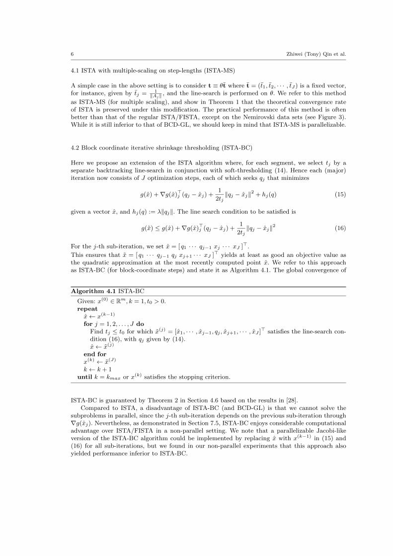
4.2 Block coordinate iterative shrinkage thresholding (ISTA-BC)

Here we propose an extension of the ISTA algorithm where, for each segment, we select tj by aseparate backtracking line-search in conjunction with soft-thresholding (14). Hence each (major)iteration now consists of J optimization steps, each of which seeks qj that minimizes

g(x) +∇g(x)>j (qj − xj) +1

2tj‖qj − xj‖2 + hj(q) (15)

given a vector x, and hj(q) := λ‖qj‖. The line search condition to be satisfied is

g(x) ≤ g(x) +∇g(x)>j (qj − xj) +1

2tj‖qj − xj‖2 (16)

For the j-th sub-iteration, we set x = [ q1 · · · qj−1 xj · · · xJ ]>.

This ensures that x = [ q1 · · · qj−1 qj xj+1 · · · xJ ]> yields at least as good an objective value asthe quadratic approximation at the most recently computed point x. We refer to this approachas ISTA-BC (for block-coordinate steps) and state it as Algorithm 4.1. The global convergence of

Algorithm 4.1 ISTA-BC

Given: x(0) ∈ Rm, k = 1, t0 > 0.repeatx← x(k−1)

for j = 1, 2, . . . , J doFind tj ≤ t0 for which x(j) = [x1, · · · , xj−1, qj , xj+1, · · · , xJ ]> satisfies the line-search con-dition (16), with qj given by (14).x← x(j)

end forx(k) ← x(J)

k ← k + 1until k = kmax or x(k) satisfies the stopping criterion.

ISTA-BC is guaranteed by Theorem 2 in Section 4.6 based on the results in [28].Compared to ISTA, a disadvantage of ISTA-BC (and BCD-GL) is that we cannot solve the

subproblems in parallel, since the j-th sub-iteration depends on the previous sub-iteration through∇g(xj). Nevertheless, as demonstrated in Section 7.5, ISTA-BC enjoys considerable computationaladvantage over ISTA/FISTA in a non-parallel setting. We note that a parallelizable Jacobi-likeversion of the ISTA-BC algorithm could be implemented by replacing x with x(k−1) in (15) and(16) for all sub-iterations, but we found in our non-parallel experiments that this approach alsoyielded performance inferior to ISTA-BC.


The FISTA update can be incorporated into the ISTA-BC algorithm. We have implementedsuch an update (FISTA-BC), but it did not exhibit any computational advantage in our tests.It is also unclear if there is any theoretical advantage in using an acceleration step in the blockcoordinate framework.

4.3 Hybrid Implementation (BCD-HYB)

We have also implemented a hybrid version of BCD-GL and ISTA-BC to overcome BCD-GL’sweakness in scalability when a data set has large groups. Specifically, we switch from a BCD sub-iteration to an ISTA-BC sub-iteration when a group contains more than NBC variables, so thatwe no longer need to perform an eigen-decomposition for that group. Clearly, this decision can bemade a priori. We call this hybrid version BCD-HYB in our experiments. The global convergenceof BCD-HYB is also established in Section 4.6.

Note that ISTA-BC and BCD-GL are identical when A>j Aj = LjI and tj = 1Lj

, where Lj is a

scalar, as in the MMV problem in Section 5. The proofs of the theoretical rates of convergence ofthe ISTA/FISTA algorithms do not readily extend to ISTA-BC or BCD-GL.

4.4 Randomized Scheme for Coordinate Selection

Nesterov recently proposed a randomized coordinate selection scheme for the BCD algorithmssolving problems with a smooth objective function [19]. Specifically, the index i of the group ofvariables xi to be optimized over in the next iteration is selected with probability

p(i)α =Lαi∑Jj=1 L

αj

, i = 1, · · · , J, (17)

where α ∈ R, and Lj is the Lipschitz constant of ∇xjg(x), the gradient of g(x) with respect tothe j-th group. When α = 0, the group indices are sampled from a uniform distribution, and whenα = 1, the probability of selecting j ∈ [1, J ] is proportional to Lj . The convergence rate resultsin [19] have been extended to the case of a composite function with a non-smooth block-separablecomponent [22], such as the Group Lasso. We implemented several versions of ISTA-BC, BCD-GL,and BCD-HYB with this randomized scheme for the special cases of α = 0 and 1. Note that the caseof α = 1 only applies for BCD-GL, where the entire set {Lj}Jj=1 is explicitly computed. We denoteby ISTA-RBC, RUBCD-GL, RBCD-HYB, the randomized versions of ISTA-BC, BCD-GL, andBCD-HYB respectively with a uniform distribution, and by RBCD-GL, the randomized version ofBCD-GL for the case where α = 1. We compare the performance of the randomized versions withthe original versions on selected problems in Section 7, and we observe that none of the versionswith a uniform distribution provides any computational advantage. On the other hand, RBCD-GLsometimes appears to be more efficient than BCD-GL.

4.5 Convergence Rate Analysis for ISTA-MS

We prove that ISTA-MS with backtracking line-search has a global convergence rate of O( 1k ), where

k is the number of iterations. Our arguments follow closely those in [2].

Define

L = [L1, L2, · · · , LJ ] =

[1

t1,

1

t2, · · · , 1

tJ

]. (18)


Corresponding to g(·) and h(·) defined in the previous sections, we define

gj : Rmj → R, gj(zj ;x) =1

2z>j A

>j Ajzj + (

∑i6=j

Aixi − b)>Ajzj , (19)

hj : Rmj → R, hj(zj) = λ‖zj‖. (20)

For each j, let L(gj) = ‖Aj‖2 be the Lipschitz constant for ∇gj . Let L(g) be the vector of the J

Lipschitz constants. Define L(g) = maxj L(gj), L(g) = minj L(gj), RL = L(g)L(g) , and sj =

√L(gj).

For ISTA-MS, the optimization problem that we solve in each iteration is

minzQMS

L (z, x) ≡ g(x) +∇g(x)>(z − x) +J∑j=1

Lj2‖zj − xj‖2 + h(z), (21)

whose solution ispMS

L (x) = St(d(x)) = arg minzQMS

L (z, x). (22)

Hence, x(k+1) = pMS

L (x(k)). Since (21) is strongly convex, we have the following property for anyx ∈ Rm from the optimality conditions for pMS

L (x):

∇g(x) + diag(L)>(pMS

L (x)− x) + ∂h(pMS

L (x)) = 0. (23)

From the definitions (19) and (20), it is easy to see that the objective function in the j-th sub-problems of ISTA-MS is a quadratic approximation of gj(zj , x

(k)) + hj(zj), where x(k) is the k-thiterate. Similar to Lemma 2.3 in [2], we have the following result.

Lemma 1 Let x ∈ Rm and L � 0 satisfy

F (pMS

L (x)) ≤ QMS

L (pMS

L (x), x). (24)

Then, for any y ∈ Rm,

F (y)− F (pMS

L (x)) ≥J∑j=1

Lj2‖pMS

L (x)j − xj‖2 + Lj(xj − yj)T (pMS

L (x)j − xj). (25)

Proof The proof follows close that in [2], except that a vector L instead of a scalar L is used, andLemma 2.2 in [2] is replaced with (23). ut

To obtain a lower bound tmin for the unscaled step-length in the k-th iteration t(k)(= θ in Section4.1), we observe that since ∇g(x) is Lipschitz continuous with Lipschitz constant L(g),

g(pMS

L (x)) ≤ g(x) +∇g(x)>(pMS

L (x)− x) +L(g)

2‖pMS

L (x)− x‖2.

If we set t(k) such that L(k)j =

sjt(k) ≥

min{sj}t(k) = L(g) ∀j, then the line-search condition is

guaranteed to be satisfied, since L(g)2 ‖p

MS

L (x(k+1))−x(k)‖2 ≤∑j

L(k)j

2 ‖pMS

L (x(k+1))j−x(k)j ‖2. Hence,

tmin =min{sj}L(g) =

√L(g)

L(g) .

With the above intermediate results, we now prove the O( 1k ) global convergence rate for ISTA-

MS.

Theorem 1 Let {x(k)} be the sequence generated by ISTA-MS. Then for any k ≥ 1,

F (x(k))− F (x∗) ≤ C

k, (26)

where x∗ is the optimal solution, and C = L(g)2

√RL‖x∗ − x(0)‖2.


Proof Applying Lemma 1 with y = x∗, x = x(n), and L = L(n), we have

2t(n)(F (x∗)− F (x(n+1))) ≥∑j

sj(‖x∗ − x(n+1)‖2 − ‖x∗ − x(n)‖2)

Since F (x∗)−F (x(n+1)) ≤ 0, we can replace t(n) with tmin. Summing the resulting inequality overn = 0, · · · , k − 1 yields

2√L(g)

L(g)

(kF (x∗)−

k−1∑n=0

F (x(n+1))

)≥∑j

sj(‖x∗j − x

(k)j ‖

2 − ‖x∗j − x(0)j ‖

2). (27)

Now, applying Lemma 1 again with x = y = x(n) and L = L(n), we get

2t(n)(F (x(n))− F (x(n+1))

)≥∑j

sj‖x(n)j − x(n+1)j ‖2.

Since this implies that F (x(n)) ≥ F (x(n+1)) for all n, it follows that∑k−1n=0 F (x(n+1)) ≥ kF (x(k)).

Combining this with (27) yields

2k√L(g)

L(g)

(F (x∗)− F (x(k))

)≥∑j

sj(‖x∗j − x

(k)j ‖

2 − ‖x∗j − x(0)j ‖

2).

Ignoring the non-negative term on the RHS of the above inequality and noting that maxj{sj} =√L(g), we obtain (26) where C = βL(g)

2

√RL‖x∗ − x(0)‖2, and L(g) is the Lipschitz constant of

∇g(x). ut

4.6 Global Convergence of BCD-HYB

We prove the global convergence of BCD-HYB by demonstrating that ISTA-BC and BCD-GL stepssatisfy the conditions on the steps of the general convergent BCGD framework in [28].

First, we briefly describe the BCGD algorithm. The blocks xj ’s are chosen in a cyclic manner.We slightly abuse the notation by calling the iteration in which xj is updated the j-th iteration.In the j-th iteration, we compute the search direction (in the subspace of xj)

dHjj= arg min

dj

(∇g(xj)

>dj +1

2d>j Hjjdj + λ‖xj + dj‖

). (28)

Here, Hjj is some approximation of the j-th diagonal block of ∇2g(x), and we denote by H(j)

the approximate Hessian used in the j-th iteration with H(j)jj = Hjj . Once the search direction

dHjjis computed, BCGD determines an appropriate step-length α(j) such that the new iterate

x(j) = x(j−1) + α(j)d(j) satisfies the following modified Armijo rule:

F (x(j)) = F (x(j−1) + α(j)d(j)) ≤ F (x(j−1)) + α(j)σ∆(j), (29)

where d(j) has its j-th segment equal to dHjjand zeros everywhere else, 0 < σ < 1, 0 ≤ γ < 1, and

∆(j) = ∇g(x)>d(j) + γ(d(j))>H(j)d(j) + λ‖x(j−1) + d(j)‖ − λ‖x(j−1)‖. (30)

It is shown in [28] that the BCGD algorithm converges globally for any choice of H(j), if theabove Armijo rule holds and if

θI � H(j) � θI ∀j, where 0 < θ ≤ θ. (31)


Our BCD-HYB algorithm differs from BCGD in that while BCGD computes the search directionand the step-length in two separate stages, BCD-HYB accomplishes both tasks in one single stage.However, as we show below, both the ISTA-BC and BCD-GL steps in BCD-HYB can be viewed asinstances of a BCGD step, and they satisfy the two conditions ((29) and (31)) above. Hence, theconvergence results of BCGD apply to our BCD-HYB algorithm.

Let us first consider the ISTA-BC steps. We observe that in this case the optimization problem(15) solved during the ISTA-BC steps is essentially identical to (28) solved by BCGD steps withHjj = 1

tjI. In addition, we see that our ISTA-BC line-search descent condition (16) agrees with the

Armijo rule descent condition (29), with α(j) = 1 ∀j, σ = 1, and γ = 0.5. Hence, from the viewpointof BCGD, ISTA-BC chooses in the j-th iteration an appropriate tj so that, with the resultingHjj = 1

tjI, the search direction dHjj

from (28) satisfies the descent condition (16) automatically.

The line-search effort in this case is shifted towards choosing an appropriate tj .In the case of BCD-GL, the steps (2) are equivalent to (28) with Hjj = Mj , which is the true

Hessian for the j-th block. Hence, F (x(j)) = F (x(j−1)) +∆(j). From the previous paragraph, it isapparent that BCD-GL always satisfies the Armijo rule with α(j) = 1 ∀j, σ = 1, and γ = 0.5.

In both cases, it is easy to see that ∆ ≤ 0 in (29), which means that if (29) is satified withσ = 1 then it also holds for any 0 < σ < 1. Hence, both ISTA-BC and BCD-GL steps satisfy themodified Armijo rule.

Now we show that steps of both types satisfy (31). Without loss of generality, assume t0 = 1 inAlgorithm 4.1. Then, tj obtained from the backtracking line-search in the j-th iteration of ISTA-BCsatisfies max{L(gj), 1} ≥ 1

tj≥ 1. From the BCGD perspective, we effectively set H(j) = 1

tjIm as

explained above. Hence, we have max{L(g), 1}Im � H(j) � min{L(g), 1}Im ∀j, and condition (31)is satisfied.

For the BCD-GL steps, we essentially set H(j) = diag(M1, · · · ,MJ). Unlike the ISTA-BC case,we only have L(g)Im � H(j) � 0, which may not satisfy (31). Hence, in the cases when Mj

is not positive definite (which only happens if columns of A from the same group are linearlydependent), we can apply the following simple modification: Hjj = Mj + δI, where δ is a smallpositive constant. The solution to the perturbed subproblem still satisfies the Armijo rule, and wenow have (L(g) + δ)Im � H(j) � δI, which satisfies (31). Hence we have shown that both types ofsteps can be viewed as those of the BCGD framework in [28], and thus the convergence results forBCGD apply. The computational performance of BCD-HYB is, however, significantly better thanthat of BCGD. We summarize the global convergence of BCD-HYB as follows.

Lemma 2 For any tj > 0, x(j−1) is a stationary point of F if and only if d(j) = 0.

Theorem 2 Let {x(j)}, {d(j)}, {tj} be sequences generated by BCD-HYB. Then the following re-sults hold.

1. {F (x(j))} is non-increasing, and ∆(j) satisfies

−∆(j) ≥ 1

2(d(j))TH(j)d(j) ≥ 1

2‖d(j)‖2 ∀j, (32)

F (x(j+1))− F (x(j)) ≤ ∆(j+1) ≤ 0 ∀j. (33)

2. If {x(j)}K is a convergent subsequence of {x(j)}, then {∆(j)} → 0 and {d(j)}K → 0.3. If the blocks are chosen in a cyclic manner, then every cluster point of {x(j)} is a stationary

point of F .4. If limj→∞ F (x(j)) ≥ −∞, then {∆(j)} → 0 and {d(j)} → 0.

The condition in the last point of Theorem 2 is always satisfied since F (x(k)) = 12‖Ax

(k) − b‖2 +

λ∑Jj=1 ‖x

(k)j ‖ ≥ 0.


5 Multiple Measurement Vector Recovery (MMV)

The basic compressed sensing aims to recover an unknown sparse signal vector from a single mea-surement vector [6][9] and is called the single measurement vector (SMV) model. The MMV model[7] extends the SMV model to reconstruct a signal matrix X =

(X1 · · · XK

)from the data matrix

A ∈ Rn×m and a matrix of multiple measurement vectors B =(B1 · · · BK

)∈ Rn×K , which are

related by AX = B. The signal (column) vectors {Xi}Ki=1 are assumed to be jointly sparse, i.e.they have non-zero entries concentrated in common rows. The convex relaxed version of the MMVmodel solves the optimization problem

minX‖X‖1,2 (34)

s.t. AX = B,

where ‖X‖1,2 =∑i ‖x

i‖2 and xi is the i-th row of X. Several methods have been proposed forsolving the MMV problem (34); e.g., see [3][4][25]. In [4], the noisy version of (34),

minX‖X‖1,2 (35)

s.t. ‖AX −B‖F ≤ σ

is considered.

5.1 Link to the Group Lasso

We can solve (34) by solving a series of sub-problems 1

minX‖X‖1,2 +

1

2µ‖AX −B‖2F , (36)

when µ→ 0. The solution X(k) to the k-th sub-problem serves as the starting point for the (k+1)-st sub-problem. By defining g(X) = 1

2‖AX−B‖2F , it is straightforward to apply ISTA-BC to solve

(36). The optimal solution to the j-th subproblem of (36) is given by the soft-thresholding operator

T (dj , tj) = dj

‖dj‖ max(0, ‖dj‖−µtj), where dj is the j-th row of the matrix X−diag(t)A>(AX−B).

We can also cast (36) directly as an instance of the Group Lasso. Define A to be the block-diagonal matrix with each diagonal block equal to the matrix A and x and b to be the column-vectorized form of the matrices X and B respectively:

A =

AA

. . .

A

, x =

X1

X2

...XK

, b =

B1

B2

...BK

.

It is easy to see that A and b are the input data if we are to solve (36) as the Group Lasso problem,and the corresponding solution is x. Since the rows of X are the segments, the j-th segment in xconsists of the j-th, the (n + j)-th, ..., and the ((K − 1)n + j)-th entries. We can re-arrange thecolumns of A so that the entries in x belonging to the same segment are contiguous. b remains the

1 This is equivalent to a special case of what is recently known as multi-task regression with structured sparsity[13].


same. Now, denoting the j-th segment of x by xj = (xj1, xj2, · · · , xjK)> and letting Aj be thecorresponding block in A, we have

Aj =

Aj

Aj. . .

Aj

and Aj xj =

Ajxj1Ajxj2

...AjxjK

,

where Aj is the j-th column of A.

5.2 Equivalence of ISTA-BC and BCD-GL

Since g(X) is a quadratic function in X, H = ∇2g(X) = A>A. Because of the special structure ofA as we have shown above, the j-th diagonal block of H, denoted Hjj , is a multiple of the identitymatrix:

Hjj = A>j Aj = ‖Aj‖2IK . (37)

Hjj is the true Hessian of the j-th block-coordinate of g(X). Hence, the BCD subproblem (2)has the same simple closed-form solution T (dj , tj) as ISTA-BC with tj = 1

‖Aj‖2 . In fact, it is

also equivalent to BCGD with least squares loss. The equivalence relationships imply that theresulting algorithm does not require the eigenvalue decompositions in BCD-GL or the backtrackingline-search in ISTA-BC, and hence, it can be very efficient. We state this specialized version inAlgorithm 5.1 (BCD-MMV).2

Algorithm 5.1 BCD-MMV

1: Given: X(0) ∈ Rm, A ∈ Rn×m, B ∈ Rn×K .2: sj ← ‖Aj‖2, j = 1, . . . ,m.3: repeat4: X ← X(k−1)

5: for j = 1, 2, . . . ,m do6: w ← sj x

j −A>j (AX −B), where xj is the j-th row of X.

7: z ← T (‖w‖sj ,1sj

), where T (·, ·) is defined in (11).

8: X(j) ←

x1

...

xj−1

z

xj+1

...xm

9: X ← X(j)

10: end for11: X(k) ← X(m)(= X)12: k ← k + 113: until k = kmax or X(k) satisfies the stopping criterion.

2 This algorithm coincides with the M-BCD method proposed in [21] recently while the first version of thispaper was in preparation.


6 Implementation

In ISTA-BC, we use back-tracking line search to determine the value(s) for t. At the beginning ofeach sub-iteration for ISTA-BC, we allow the initial step-length to increase from the previous stepsize for that segment by a factor of 1

β , where 0 < β < 1.

The major computational work of the line-search performed by ISTA-BC (and FISTA-BC) liesin computing the residual r = Ax − b. In the j-th sub-iteration only the j-th segment of x isupdated. Hence, we can update the residual incrementally as Ax − b = Aj(zj − xj) + (Ax − b).The old residual Ax − b is available before the sub-iteration, so the total work of this scheme ison average 1

J of the work required to compute Ax − b from scratch, where J is the total numberof segments. To avoid the accumulation of arithmetic errors over many iterations, we compute theactual residual every J sub-iterations.

We set NBC = 200 for our BCD-HYB implementation discussed in Section 4.3. In Algorithm2.1, the initial value of ∆ was set at 0 for the first iteration of Newton’s method. The result of eachiteration was then used as the initial value for the next iteration.

7 Numerical Experiments

All numerical experiments were run in Matlab on a laptop with an Intel Core 2 Duo CPU and 4Gmemory. We recorded the CPU times, the number of matrix-vector multiplications (Aprods), andthe number of major iterations (Iters) required by each of the algorithms discussed in the previoussections on the test sets. We implemented a version of BCGD [28] in which the blocks are chosenby the Gauss-Seidel rule, to compare with our methods. We also ran publicly available software forSPARSA [31], SLEP3 [15], and SPOR-SPG4 [4] on our test problems. Both SPARSA and SLEPsolve the unconstrained formulation of the Group Lasso, while SPOR-SPG solves the constrainedversion. Since the SLEP solver has its core sub-routine (the Euclidean projection [14]) implementedin the C language, and so does SPOR-SPG for its one-norm projection [5], the Aprods serves as abetter measure of performance than CPU times.

The stopping criterion ‖Gt(x)‖ = ‖1t (x− pt(x))‖ ≤ ε is suggested in [30] and can be applied to

all ISTA/FISTA versions. We observed that ε = 10−2 was sufficient to recover the sparse solutionsin our experiments. However, for comparison we used a different criterion which we explain belowin Sections 7.3 and 7.4. The penalty parameter λ was chosen as γλmax, where λmax is the upperbound derived in [17]. We chose γ = 0.2, which we found to yield reasonable level of group sparsityin general.

For the ease of recalling the names of the algorithms introduced in Sections 2 - 4, we summarizethe abbreviated names in Table 1 below.

7.1 Synthetic Data Sets

We tested the algorithms on simulated problems of various sizes. Tables 2, 3, and 4 present theattributes of the Group Lasso and the MMV standard data sets respectively. Data sets yl1 to yl4are from [33]; mgb1 and mgb2 are from [17]; ljy is adapted from a test set in [15]; nemirovski1-4were created by Nemirovski and made challenging for the first-order methods, in the spirit of theworst case complexity examples. The MMV data sets in Table 4 are the ones in the online appendixof [4], and the comprehensive scalability test sets are adapted from the one in [25]. We refer thereaders to Appendix A for the details of the simulated data sets.

3 We ran only the Group Lasso experiments on SLEP.4 We ran the MMV experiments on SPOR-SPG [4] and the Group Lasso experiments on SPG in [5].


Abbrev. names Algorithms

ISTA-BC Algorithm 4.1FISTA-BC ISTA-BC with the FISTA updateISTA-MS ISTA with multi-scaling on step-lengths (Section 4.1)BCD-GL Algorithm 2.1

BCD-HYB Hybrid version of BCD-GL and ISTA-BC (Section 4.3)RBCD-GL Randomized BCD-GL with probability distribution

proportional to block-wise Lipschitz constantsRUCBD-GL Randomized BCD-GL with uniform distributionISTA-RBC Randomized ISTA-BC with uniform distribution

RBCD-HYB Randomized BCD-HYB with uniform distribution

Table 1 Summary of the abbreviated names of the algorithms.

Data set n J m (no. features) Data type

yl1 50 15 15×3 categorical

yl2 100 10 4×2+6×4 categorical

yl3 100 16 16×2 continuous

yl4 500 100 50×3+50×2 mixed

mgb1 200 4 1+3×3 continuous

mgb2 100 251 1+250×4 continuous

ljy 1000 100 100×10 continuous

nemirovski1 1036 52 1036 continuous




Table 2 Synthetic data sets. n = no. samples, J = no. of segments. The fourth column indicates the group sizesand the number of groups for each size.

7.2 Breast Cancer Data Set

To demonstrate the efficiency of our proposed algorithms on real-world data, we used the breastcancer data set [29] to compare their performance with that of existing algorithms on a regressiontask of predicting the patients’ lengths of survival. This data set contains gene expression profilingdata for 8141 genes in 295 breast cancer tumors. We considered only those genes with knownsymbols. There are various approaches in the literature for grouping the genes by their functions.We followed [11] and used the canonical pathways from MSigDB [24], which contains 880 genegroups. 878 out of these groups involve the genes studied in the breast cancer data set, accountingfor 3510 genes. Note that the gene groups may overlap. However, by adopting the model proposedin [11], we were able to still solve a classical Group Lasso problem by augmenting the design matrixas in [11], increasing the total number of features to 28459.

7.3 Group Lasso experiments

To obtain a fair comparison of the computational performance among all the algorithms, we pre-computed a reference solution x∗ for each problem and stopped the algorithms when the current


Data set n J m (no. features) Data type

yl1L 5000 50 47×10+3×1000 categorical

yl4L 2000 114 50×3+4×1000+50×3+10×50 mixed

mgb2L 2000 6 1+5×1000 continuous

ljyL 2000 15 5×200+10×500 continuous

glasso5 1000 400 3000 mixed

glassoL1 2000 242 10000 continuous

glassoL2 4000 438 20000 continuous

Table 3 Synthetic data sets. These test sets have much larger groups and more samples than the ones in Table2.

Data set A K No. nnz rows ν σ

mmv1a 60 × 100 5 12 0.01 1.0‖R‖Fmmv1d 200 × 400 5 20 0.01 1.2‖R‖Fmmv1e 200 × 400 10 20 0.02 1.0‖R‖Fmmv1f 300 × 800 3 50 0.01 0.9‖R‖F

Table 4 MMV data sets. The noisy measurement matrix B = AX0 + R, where X0 is the ground truth signalmatrix and R is the noise matrix with ‖R‖ = ν‖AX0‖F .

Data set n (no. meas) m (no. groups) K (group size) sparsity

spa 100 500 10 25:25:250

meas 100:100:1000 600 20 30

compreh 10,40:40:200 4n 2n 10% × m

Table 5 MMV scalability test data sets. The measurement matrices are noiseless. We adopt the Matlab syntaxa : b : c to represent the sequence from a to c with increments of b.

solution x satisfied F (x) − F (x∗) ≤ 10−5. For SPG, we used x∗ to compute the appropriateparameter value τ(= ‖x∗‖1,2) required by the solver, and we set the projected gradient toleranceat 10−3. The reference solutions were obtained by running ISTA-BC to the point where the relativechange in the objective value is less than 10−10. We also performed a convergence rate test on thebreast cancer data set.

Since the matrix-vector multiplications performed by ISTA-BC, BCD-HYB, and BCGD involveonly a block of the matrix A each time, e.g. A>j r(r ∈ Rn) and Ajxj , we treated each of thesemultiplications as a fraction of a unit Aprods. Hence, the Aprods counts for these algorithms werefractional.

7.4 The MMV experiments

For all the algorithms except SPOR-SPG, we used continuation for solving the MMV test problems.The problems in Table 4 contain noisy measurements. Hence, the noisy version (35) has to be solved.We used ISTA-BC to compute the reference solutions for the MMV data sets in Table 4 in the same


way as for the Group Lasso experiments (with continuation), and we recorded the correspondingµ’s for which the solution obtained to problem (36) satisfies ‖AX −B‖F ≤ σ, for the given σ’s inTable 4. We compared the performance of the algorithms in the same way as in the Group Lassoexperiments. Besides the standard comparisons, we performed several scalability tests to see howthe test statistics changed with variations in individual dimensions of the problem input data. Asummary of the scalability test attributes is given in Table 5. The measurements are all noiseless.For these scalability tests, we allowed the algorithms to run until the objective function values‖X‖1,2 converged to a relative accuracy of 10−5. A reference solution is not required in this case.The results for the MMV tests are summarized in Figure 6.

The number of matrix-vector multiplications is counted in a slightly different way from thatin the Group Lasso experiments. Here, the basic computations involved in ISTA-BC/FISTA-BC and BCD-MMV are A>j R for computing the gradient and Ajx

j for the incremental resid-

ual update, while SPARSA and SPOR-SPG both have A>R and AX as basic computations.Recall that Aj is the j-th column of A and xj is the j-th row of X in the MMV case. SinceA>R = [A>R1 . . . A

>RK ], and AX = [AX1 . . . AXK ], each A>R and AX actually involves K

matrix-vector multiplications. So, Aprods = K(#(A>R) + #(AX)) = Km (#(A>j R) + #(Ajx

j)).

7.5 Results

Because of space consideration and the number of algorithms that we compared, we present ourresults using the performance profiles proposed by Dolan and More [8]. For any given algorithmA, these profiles plot for each value of a positive factor τ the percentage of problems (from thegiven problem set) on which the performance of A is within a factor of τ of the best performanceof any algorithm on this problem. Hence, when the plot of algorithm A is shifted more towards theleft in the figure than another algorithm’s plot, it indicates that algorithm A solves more problemsquicker. If the plot is shifted more towards the top, this indicates that algorithm A is more robust.

We present the performance profiles for the Group Lasso experiments in Figure 1. We alsopresent convergence plots in Figure 2. It should be noted that the eigen-decompositions and New-ton’s root-finding steps for BCD-GL are not reflected in Aprods. The cost of the two procedures issmall compared to the total cost per iteration when the group sizes are small. For data sets withlarge groups, Aprods for BCD-HYB gives a more accurate representation of the CPU performance.Hence, we have included BCD-HYB instead in Figure 1 for better comparison. Figure 6 summarizesthe MMV test results.

7.5.1 Group Lasso

The performance profile plots show that BCD-HYB and ISTA-BC clearly outperform FISTA andBCGD overall. BCD-HYB yields some of the best results in terms of Aprods and the number ofiterations for the small data sets. The results for the large data sets are less clear-cut, but BCD-HYBis competitive against the other existing algorithms. This is evident from Figures 3 and 4.

Although ISTA-BC carries out a separate line-search for each segment of x, the considerablegain in computational performance often justifies the extra cost of the line-search. This is, however,not the case on the Nemirovski data sets, where ISTA-BC, ISTA-MS, and BCGD performed muchworse than the rest of the group. It is interesting to observe that applying the FISTA step in theblock coordinate case does not benefit computational performance on a number of Group Lassodata sets.

On the real-world breast cancer data set, we see from the convergence plot that BCD-HYB,ISTA-BC, and SPG are best and comparable to each other, with BCD-HYB and ISTA-BC havinga marginal advantage (see also Figure 5). FISTA-BC, FISTA, and SLEP show roughly the samerate of convergence, while the remaining algorithms form another group exhibiting a different


Fig. 1 Performance profiles graph [8] for the Group Lasso data sets.

Fig. 2 Group Lasso convergence rate test on the breast cancer gene expression data set. The performances ofBCD-HYB and ISTA-BC are almost identical.

convergence rate. Again, it is an interesting observation that the FISTA group actually exhibits alower empirical rate of convergence.

We tested the randomized algorithms discussed in Section 4.4 on selected problems in Tables2 and 3 as well as the breast cancer data set. From the results in Table 6, it appears that therandomized algorithms with a uniform distribution have no computational advantage over theiroriginal counterparts. RBCD-GL with a distribution where the probabilities are proportional tothe corresponding group-wise Lipschitz constants shows better performance in terms of the numberof iterations, but it has the same disadvantage of having to perform eigen-decomposition as BCD-GL on instances with large groups.

7.5.2 MMV

We did not include the results of SPARSA in Figure 6 because it consistently stopped at suboptimalsolutions for the scalability tests. From Figure 6, it is clear that FISTA-BC and BCD-MMV have an


Fig. 3 Performance comparison for the small Group Lasso data sets.

Fig. 4 Performance comparison for the large Group Lasso data sets. The bars corresponding to the algorithmsthat did not terminate within the maximum number of iterations are assigned to a value of 10,000.


Fig. 5 Breast cancer data test results. The reference solution is computed by ISTA-BC. The target accuracyhere is 10−5.

Fig. 6 MMV test results.


Data Sets Algs CPU (s) Iters Aprods

yl3

ISTA-BC 1.82e-001 20 8.30e+001BCD-HYB 1.02e-001 6 2.13e+001BCD-GL 3.29e-001 8 2.84e+001

RBCD-GL 2.08e-001 15 4.97e+001RUBCD-GL 1.85e-001 16 5.28e+001ISTA-RBC 3.27e-001 20 8.13e+001

RBCD-HYB 5.75e-001 10 3.34e+001

yl4

ISTA-BC 6.63e-001 27 1.02e+002BCD-HYB 5.21e-001 21 6.57e+001BCD-GL 5.01e-001 21 6.67e+001

RBCD-GL 5.39e-001 15 5.45e+001RUBCD-GL 6.67e-001 32 9.97e+001ISTA-RBC 1.12e+000 33 1.26e+002

RBCD-HYB 7.92e-001 30 9.27e+001

glassoL1

ISTA-BC 7.63e+001 451 1.79e+003BCD-HYB 5.86e+001 349 1.17e+003BCD-GL 5.26e+001 316 1.07e+003

RBCD-GL 1.17e+002 544 1.90e+003RUBCD-GL 1.05e+002 604 1.96e+003ISTA-RBC 1.45e+002 810 3.20e+003

RBCD-HYB 1.17e+002 665 2.17e+003

glassoL2



RBCD-HYB 1.97e+002 307 1.04e+003

BreastCancerData



RBCD-HYB 4.34e+001 214 7.57e+002

Table 6 Numerical results on selected problems for the randomized algorithms and their original counterparts.ISTA-RBC, RUBCD-GL, RBCD-HYB are the randomized versions of ISTA-BC, BCD-GL, and BCD-HYB re-spectively with a uniform distribution, and RBCD-GL is the randomized version of BCD-GL with a distributionwhere the probabilities are proportional to the group-wise Lipschitz constants {Lj}Jj=1.

advantage over the FISTA in terms of Aprods. BCD-MMV is very competitive against SPOR-SPGand, in many cases, performed better. In the scalability test on sparsity level, however, both FISTAand BCD-MMV appear to be invariant to the increase in the sparsity level, while FISTA-BC andSPOR-SPG require increasing amount of computation.


8 Conclusion

We have proposed a general version of the BCD algorithm for the Group Lasso as well as anextension of ISTA based on variable step-lengths. The combination of the two yields an efficientand scalable method for solving the Group Lasso problems with various group sizes. As a specialcase, we have also considered the MMV problem and applied the ISTA-BC/BCD algorithm to it.Our numerical results show that the proposed algorithms compare favorably to current state-of-the-art methods in terms of computational performance.

Acknowledgements The authors would like to thank Shiqian Ma for valuable discussions on the MMV problems.

References

1. Bach, F.: Consistency of the group Lasso and multiple kernel learning. The Journal of Machine LearningResearch 9, 1179–1225 (2008)

2. Beck, A., Teboulle, M.: A fast iterative shrinkage-thresholding algorithm for linear inverse problems. SIAMJournal on Imaging Sciences 2(1), 183–202 (2009)

3. van den Berg, E., Friedlander, M.: Joint-sparse recovery from multiple measurements. arXiv 904 (2009)4. van den Berg, E., Friedlander, M.: Sparse Optimization With Least-squares Constraints. Tech. rep., Technical

Report TR-2010-02, Department of Computer Science, University of British Columbia (2010)5. van den Berg, E., Schmidt, M., Friedlander, M., Murphy, K.: Group sparsity via linear-time projection. Tech.

rep., Technical Report TR-2008-09, Department of Computer Science, University of British Columbia (2008)6. Candes, E., Romberg, J., Tao, T.: Robust uncertainty principles: Exact signal reconstruction from highly

incomplete frequency information. Information Theory, IEEE Transactions on 52(2), 489–509 (2006)7. Chen, J., Huo, X.: Theoretical results on sparse representations of multiple-measurement vectors. IEEE

Transactions on Signal Processing 54, 12 (2006)8. Dolan, E., More, J.: Benchmarking optimization software with performance profiles. Mathematical Program-

ming 91(2), 201–213 (2002)9. Donoho, D.: Compressed sensing. Information Theory, IEEE Transactions on 52(4), 1289–1306 (2006)

10. Friedman, J., Hastie, T., Tibshirani, R.: A note on the group lasso and a sparse group lasso. preprint (2010)11. Jacob, L., Obozinski, G., Vert, J.: Group Lasso with overlap and graph Lasso. In: Proceedings of the 26th

Annual International Conference on Machine Learning, pp. 433–440. ACM (2009)12. Kim, D., Sra, S., Dhillon, I.: A scalable trust-region algorithm with application to mixed-norm regression. In:

Int. Conf. Machine Learning (ICML), vol. 1 (2010)13. Kim, S., Xing, E.: Tree-guided group lasso for multi-task regression with structured sparsity. In: Proceedings

of the 27th Annual International Conference on Machine Learning (2010)14. Liu, J., Ji, S., Ye, J.: Multi-task feature learning via efficient l 2, 1-norm minimization. In: Proceedings of

the Twenty-Fifth Conference on Uncertainty in Artificial Intelligence, pp. 339–348. AUAI Press (2009)15. Liu, J., Ji, S., Ye, J.: SLEP: Sparse Learning with Efficient Projections. Arizona State University (2009)16. Ma, S., Song, X., Huang, J.: Supervised group Lasso with applications to microarray data analysis. BMC

bioinformatics 8(1), 60 (2007)17. Meier, L., Van De Geer, S., Buhlmann, P.: The group lasso for logistic regression. Journal of the Royal

Statistical Society: Series B (Statistical Methodology) 70(1), 53–71 (2008)18. More, J., Sorensen, D.: Computing a trust region step. SIAM Journal on Scientific and Statistical Computing

4, 553 (1983)19. Nesterov, Y.: Efficiency of coordinate descent methods on huge-scale optimization problems. CORE Discussion

Papers (2010)20. Nocedal, J., Wright, S.: Numerical optimization. Springer verlag (1999)21. Rakotomamonjy, A.: Surveying and comparing simultaneous sparse approximation (or group-lasso) algo-

rithms. Signal processing (2011)22. Richtarik, P., Takac, M.: Iteration complexity of randomized block-coordinate descent methods for minimizing

a composite function. Arxiv preprint arXiv:1107.2848 (2011)23. Roth, V., Fischer, B.: The group-lasso for generalized linear models: uniqueness of solutions and efficient

algorithms. In: Proceedings of the 25th international conference on Machine learning, pp. 848–855. ACM(2008)

24. Subramanian, A., Tamayo, P., Mootha, V., Mukherjee, S., Ebert, B., Gillette, M., Paulovich, A., Pomeroy,S., Golub, T., Lander, E., et al.: Gene set enrichment analysis: a knowledge-based approach for interpretinggenome-wide expression profiles. Proceedings of the National Academy of Sciences of the United States ofAmerica 102(43), 15,545 (2005)

25. Sun, L., Liu, J., Chen, J., Ye, J.: Efficient Recovery of Jointly Sparse Vectors. NIPS (2009)


26. Tibshirani, R.: Regression shrinkage and selection via the lasso. Journal of the Royal Statistical Society.Series B (Methodological) 58(1), 267–288 (1996)

27. Tseng, P.: Convergence of a block coordinate descent method for nondifferentiable minimization. Journal ofoptimization theory and applications 109(3), 475–494 (2001)

28. Tseng, P., Yun, S.: A coordinate gradient descent method for nonsmooth separable minimization. Mathemat-ical Programming 117(1), 387–423 (2009)

29. Van De Vijver, M., He, Y., van’t Veer, L., Dai, H., Hart, A., Voskuil, D., Schreiber, G., Peterse, J., Roberts,C., Marton, M., et al.: A gene-expression signature as a predictor of survival in breast cancer. New EnglandJournal of Medicine 347(25), 1999 (2002)

30. Vandenberghe, L.: Gradient methods for nonsmooth problems. EE236C course notes (2008)31. Wright, S., Nowak, R., Figueiredo, M.: Sparse reconstruction by separable approximation. IEEE Transactions

on Signal Processing 57(7), 2479–2493 (2009)32. Yang, H., Xu, Z., King, I., Lyu, M.: Online learning for group lasso. In: 27th Intl Conf. on Machine Learning

(ICML2010). Citeseer33. Yuan, M., Lin, Y.: Model selection and estimation in regression with grouped variables. Journal of the Royal

Statistical Society: Series B (Statistical Methodology) 68(1), 49–67 (2006)34. Zou, H., Hastie, T.: Regularization and variable selection via the elastic net. Journal of the Royal Statistical

Society: Series B (Statistical Methodology) 67(2), 301–320 (2005)

A Simulated Data Sets

For the specifications of the data sets in Table 2, interested readers can refer to the references provided at thebeginning of Section 7.1. Here, we provide the details of the data sets in Table 3.

A.1 yl1L

50 latent variables Z1, . . . , Z50 are simulated from a centered multivariate Gaussian distribution with covariancebetween Zi and Zj being 0.5|i−j|. The first 47 latent variables are encoded in {0, . . . , 9} according to their inversecdf values as done in [33]. The last three variables are encoded in {0, . . . , 999}. Each latent variable correspondsto one segment and contributes L columns in the design matrix with each column j containing values of theindicator function I(Zi = j). L is the size of the encoding set for Zi. The responses are a linear combination of asparse selection of the segments plus a Gaussian noise. We simulate 5000 observations.

A.2 yl4L

110 latent variables are simulated in the same way as the third data set in [33]. The first 50 variables contribute3 columns each in the design matrix A with the i-th column among the three containing the i-th power of thevariable. The next 50 variables are encoded in a set of 3, and the final 10 variables are encoded in a set of 50,similar to yl1L. In addition, 4 groups of 1000 Gaussian random numbers are also added to A. The responses areconstructed in a similar way as in yl1L. 2000 observation are simulated.

A.3 mgb2L

5001 variables are simulated as in yl1L without categorization. They are then divided into six groups, with firstcontaining one variable and the rest containing 1000 each. The responses are constructed in a similar way as inyl1L. We collect 2000 observations.

A.4 ljyL

We simulate 15 groups independent standard Gaussian random variables. The first five groups are of a size 5 each,and the last 10 groups contain 500 variables each. The responses are constructed in a similar way as in yl1L, andwe simulate 2000 observations.


A.5 glassoL1,glassoL2

The design matrix A is drawn from the standard Gaussian distribution. The length of each group is sampledfrom the uniform distribution U(10, 50) with probability 0.9 and from the uniform distribution U(50, 300) withprobability 0.1. We continue to generate the groups until the specified number of features m is reached. Theground truth feature coefficients x∗ is generated from N (2, 4) with approximately 5% non-zero values, and weassume a N (0.5, 0.25) noise.

e cient block-coordinate descent algorithms for the group ... · e cient block-coordinate descent...

Documents