r t d rgccarecent advances on rgcca · pls path modeling tenenhaus m., esposito vinzi v., chatelin...

R t d RGCCARecent advances on RGCCA

Arthur Tenenhaus, Supelec

Beijing, 28/10/2011

Glioma Cancer Data(Department of Pediatric Oncology of the Gustave Roussy Institute)

Transcriptomic data (X1)

(X )

Gene 1 Gene 2 … Gene 15201 CGH1 … CGH 15201 Localization

outcome (X3)

Gene 1 Gene 2 … Gene 15201 CGH1 … CGH 15201 LocalizationPatient 1 0.18 -0.21 -0.73 0.00 -0.55 Hemisphere Patient 2 1.15 -0.45 0.27 -0.30 0.00 Midline Patient 3 1.35 0.17 0.22 0.33 0.64 DIPG

Patient 56 1.39 0.18 … -0.17 0.00 … 0.43 Hemisphere

222CGH data (X2)

Glioma Cancer Data: from a multi-block viewpoint(Department of Pediatric Oncology of the Gustave Roussy Institute)

Gene 1 … Gene 15201Ge e … Ge e 5 0Patient 1 0.18 -0.73 Patient 2 1.15 0.27 Patient 3 1 35 0 22

ξ1 C13 = 1Patient 3 1.35 0.22

Patient 56 1.39 -0.17

Hemisphere DIPG Patient 1 1 0 Patient 2 0 0 ξ3

C13 1

C = 1C = 0 CGH1 … CGH 15201 Patient 1 0.00 -0.55

Patient 3 0 1

Patient 56 1 0

ξ3

C = 1

C12 = 1C12 = 0

Patient 2 -0.30 0.00Patient 3 0.33 0.64

P ti t 56 0 00 0 43

ξ2

C23 1

Patient 56 0.00 0.43

33

References

• Paper

• PackagePackage

4

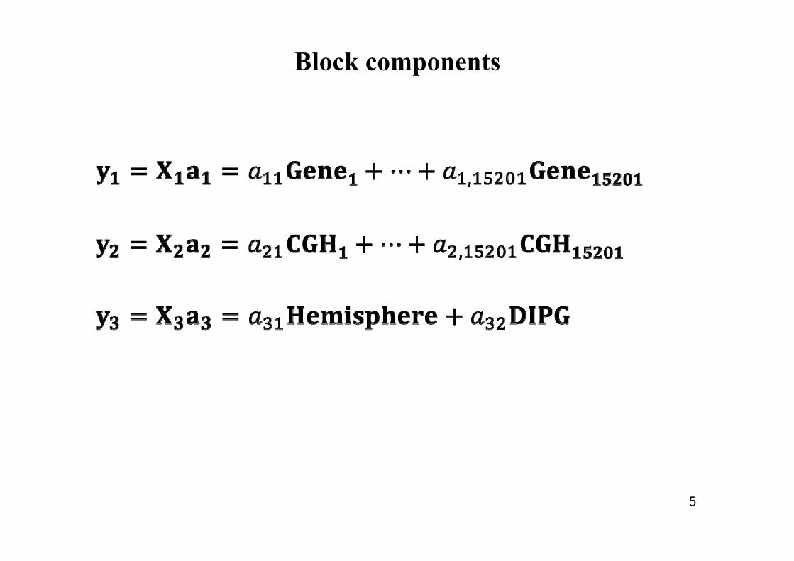
Block components

5

Covariance-based criteriaSome modified multi-block methods cjk = 1 if blocks are linked, 0 otherwise and cjj = 0

SUMCOR (Horst, 1961)

SSQCORGENERALIZED CANONICAL CORRELATION ANALYSISSSQCOR (Mathes, 1993 ; Hanafi, 2004)

SABSCOR (M th 1993 H fi 2004)

GENERALIZED CANONICAL CORRELATION ANALYSIS

SABSCOR (Mathes, 1993 ; Hanafi, 2004)

SUMCOV (Van de Geer, 1984)

SSQCOVGENERALIZED CANONICAL COVARIANCE ANALYSISSSQCOV (Hanafi & Kiers, 2006)

SABSCOV (Krämer 2006)

GENERALIZED CANONICAL COVARIANCE ANALYSIS

SABSCOV (Krämer, 2006)

Covariance-based criteriacjk = 1 if blocks are linked, 0 otherwise and cjj = 0

SUMCOR:

SSQCORSSQCOR:

SABSCOR:SABSCOR:

SUMCOV:SUMCOV:

SSQCOV:Q

SABSCOV:

7

RGGCA optimization problem

argmax g cov ,1, 2,…,

1 var 2 1, 1,… ,Subject to the constraints 1 var 1, 1,… , Subject to the constraints

⎧ connectedisandif1 XXA monotone convergent algorithml d hi i i i bl

⎩⎨⎧

=otherwise 0

connectedis andif 1 kj XXjkcwhere:related to this optimization problem

will be described.

identity (Horst sheme)

square (Factorial scheme)g

⎧⎪= ⎨square (Factorial scheme)

abolute value (Centroid scheme)

g = ⎨⎪⎩Schäfer and Strimmer formula can be used for an

optimal determination of the shrinkage constantsand: Shrinkage constant between 0 and 1jτ =optimal determination of the shrinkage constants

Construction of monotone convergent algorithms for these criteriathese criteria

• Construct the Lagrangian function related to the optimization problem.optimization problem.

• Cancel the derivative of the Lagrangian function with respect to each arespect to each aj.

• Use the Wold’s procedure to solve the stationary ti ( G S id l l ith )equations (≈ Gauss-Seidel algorithm).

• This procedure is monotonically convergent: the criterion increases at each step of the algorithm.

9

The RGCCA algorithm (primal version)

jjj aXy =

Outer Estimation(explains the block) Inner(explains the block)

( ) ( ) 1var12=+− jjjjj aaX ττInitial

step ja

InnerEstimation(explains relation

kk

jkj e yz ∑=Iterate until convergencef th it i

relation between block)

jk≠

( ) jtjjj

tjj zXIXX

111−

⎟⎞

⎜⎛ +− ττ

of the criterionChoice of weights ejh:- Horst : jkjk ce =( )

( ) jtjjj

tjjj

tj

jjjjjj

j

zXIXXn

Xz

zXIXXna

111

1

−

⎟⎠⎞

⎜⎝⎛ +−

⎟⎠

⎜⎝

+=

ττ

ττ- Centroid :

- Factorial :

( )( )kjjkjk ce yy ,corsign=

( )kjjkjk ce yy ,cov=n ⎠⎝

cjk = 1 if blocks are linked, 0 otherwise and cjj = 0

The RGCCA algorithm (dual version)

jtjjj αXXy =

InnerOuter Estimation

(explains the block)

Initialstep jα


kk

jkj e yz ∑=(explains the block)

( )[ ] 1)1( 1 =−+ jtjjnjj

tjj

tj αXXIXXα ττ

Iterate until convergencef th it i


jk≠

( ) jjtjjj zIXX

111−

⎟⎞

⎜⎛ +− ττ

of the criterionChoice of weights ejh:- Horst : jkjk ce =( )

( ) jjtjjj

tjj

tj

jjjjj

j

zIXXn

XXz

zIXXnα

111

1

−

⎟⎠⎞

⎜⎝⎛ +−

⎟⎠

⎜⎝

+=

ττ

ττ- Centroid :

- Factorial :


( )kjjkjk ce yy ,cov=n ⎠⎝


special cases of RGCCA (among others)

PLS Regression Wold S., Martens & Wold H. (1983): The multivariate calibration problem in chemistry solved by the PLS method. In Proc. Conf. Matrix Pencils, Ruhe A. & Kåstrøm B. (Eds), March 1982, Lecture Notes in Mathematics, Springer Verlag,

Heidelberg, p. 286-293.

Redundancy analysis Barker M. & Rayens W. (2003): Partial least squares for discrimination, Journal of Chemometrics, 17, 166-173.

Regularized CCA Vinod H. D. (1976): Canonical ridge and econometrics of joint production. Journal of Econometrics, 4, 147–166.

Inter-battery factor analysis Tucker L.R. (1958): An inter-battery method of factor analysis, Psychometrika, vol. 23, n°2, pp. 111-136.

MCOA Chessel D. and Hanafi M. (1996): Analyse de la co-inertie de K nuages de points. Revue de Statistique Appliquée, 44, 35-6060

SSQCOV Hanafi M. & Kiers H.A.L. (2006): Analysis of K sets of data, with differential emphasis on agreement between and withinsets, Computational Statistics & Data Analysis, 51, 1491-1508.

SUMCOR Horst P (1961): Relations among m sets of variables Psychometrika vol 26 pp 126-149SUMCOR Horst P. (1961): Relations among m sets of variables, Psychometrika, vol. 26, pp. 126 149.

SSQCOR Kettenring J.R. (1971): Canonical analysis of several sets of variables, Biometrika, 58, 433-451

MAXDIFF Van de Geer J. P. (1984): Linear relations among k sets of variables. Psychometrika, 49, 70-94.

PLS path modeling Tenenhaus M., Esposito Vinzi V., Chatelin Y.-M., Lauro C. (2005): PLS path modeling. Computational Statistics and Data(mode B) Analysis, 48, 159-205.

Generalized Orthogonal Vivien M. & Sabatier R. (2003): Generalized orthogonal multiple co-inertia analysis (-PLS): new multiblock componentMCOA and regression methods, Journal of Chemometrics, 17, 287-301.

1212Caroll’s GCCA Carroll, J.D. (1968): A generalization of canonical correlation analysis to three or more sets of variables, Proc. 76th

Conv. Am. Psych. Assoc., pp. 227-228.

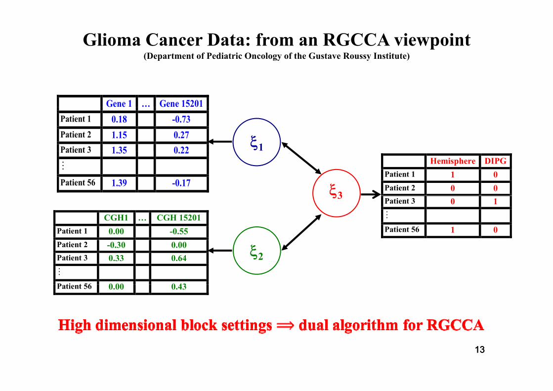
Glioma Cancer Data: from an RGCCA viewpoint(Department of Pediatric Oncology of the Gustave Roussy Institute)

Gene 1 … Gene 15201Ge e … Ge e 5 0Patient 1 0.18 -0.73 Patient 2 1.15 0.27 Patient 3 1 35 0 22

ξ1Patient 3 1.35 0.22

Patient 56 1.39 -0.17 ξ3

Hemisphere DIPG Patient 1 1 0 Patient 2 0 0

CGH1 … CGH 15201 Patient 1 0.00 -0.55

ξ3 Patient 3 0 1

Patient 56 1 0

Patient 2 -0.30 0.00Patient 3 0.33 0.64

P ti t 56 0 00 0 43

ξ2

Patient 56 0.00 0.43

131313

Bayesian Discriminant Analysis of localization on y1 and y2y1 y2

y2

15y1

Predictive performance

Observed DIPG Hemispheres Midline

Table 1. Learning phase

Predicted DIPG Hemispheres Midline

DIPG 20 0 1Hemispheres 0 19 4Midline 0 5 7

Accuracy = 82%

y2

ObservedPredicted DIPG Hemispheres Midline

Table 2. Testing phase (leave-one-out)

y2


Accuracy = 75%

y16

y1

Variable selection for RGCCA

argmax g cov ,1, 2,…,

22 1, 1, … ,

Subject to the constraints1

, 1, … ,Subject to the constraints

⎧ connectedisandif1 XX

⎩⎨⎧

=otherwise 0

connectedis andif 1 kj XXjkcwhere:

identity (Horst sheme)

square (Factorial scheme)g

⎧⎪= ⎨square (Factorial scheme)

abolute value (Centroid scheme)

g = ⎨⎪⎩

and: Shrinkage constant between 0 and 1jτ =

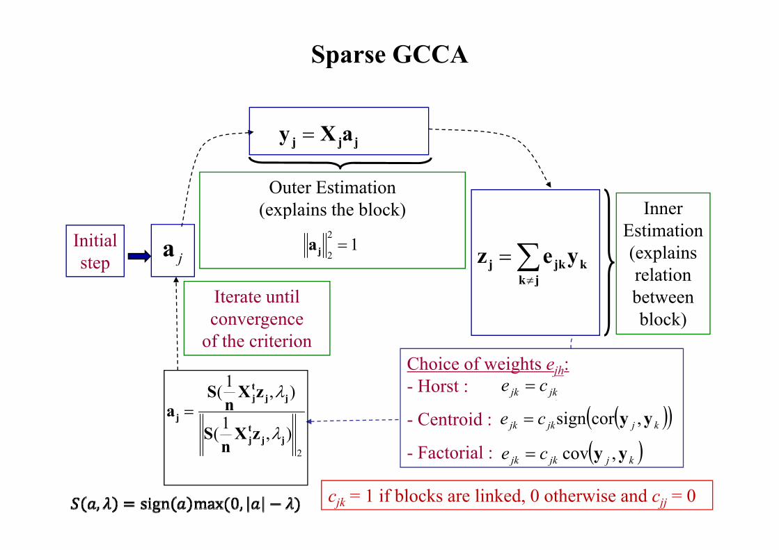
Sparse GCCA

jjj aXy =

Outer Estimation(explains the block) Inner(explains the block)

12

2=jaInitial

step ja


kjkj yez ∑=Iterate until convergencef th it i


jk≠

of the criterionChoice of weights ejh:- Horst : jkjk ce =),1( jj

tjzXS λ

- Centroid :

- Factorial :


( )kjjkjk ce yy ,cov=2

),1(

),(

jjtj

jjj

j

zXn

S

naλ

=


( )kjjkjk yy

List of selected variables from GE data

FOXG1 PTPN9 CYP4Z1 ARFGAP3 KRAS TMEM19

List of selected variables from CGH data

STK38L BBS10FOXG1 PTPN9 CYP4Z1 ARFGAP3ZFHX4 WNT5A PI16 PDLIM4EEPD1 COL10A1 TRIM43 VIPR2GRID2 PBX3 BTC ACADLEMX1 TKTL1 PKNOX2 LAMB3

KRASAPOLD1CDKN2BCDKN2ACNOT2

TMEM19HEBP1BHLHE41C12orf36RAB21

STK38LCAPRIN2SOX5AMN1THAP2

BBS10TSPAN11GPRC5DGPRC5ADENND5BEMX1 TKTL1 PKNOX2 LAMB3

DLX2 LY6D SERPINB10 DCAF6ITM2C CRYGD TAAR2 NET1SEMA3D HOXA3 ZNF469 ELOVL2PTHLH KRTAP9 9 FAM196B DAAM2

CNOT2ABCC9CAPS2IAPPPPFIBP1

RAB21C12orf72GSG1C9orf53GLIPR1

THAP2PYROXD1PHLDA1CSRP2KRR1

DENND5BNAP1L1KLHDC5DDX47C12orf28PTHLH KRTAP9-9 FAM196B DAAM2

RASL12 LHX1 SLC22A3 CHCHD7PPAPDC1A ZNF483 HOXB2 FAIMHCG4 NLRP7 SLC25A2 HOXA2TRIM16L ABI3BP HES4 SPEF2

PPFIBP1NAV3SLCO1A2PTHLH

GLIPR1PTPRBE2F7KIAA0528LGR5

KRR1PTPRRTM7SF3ZFC3H1CCDC91

C12orf28LDHBFAR2ST8SIA1LRMPTRIM16L ABI3BP HES4 SPEF2

NR0B1 MCF2 SYT9 C8orf47LHX2 SATB2 C2orf88 DLEC1RNF182 HTR1D CLDN3 FZD7

ELK3KIAA1467ETNK1RAB3IP

LGR5ZDHHC17MRPS35C12orf70TBC1D15

CCDC91KCNC2SLCO1B1BCAT1

LRMPEMP1C12orf11OSBPL8KCNJ8KIAA0556 LOXHD1 GLUD2 PLIN4

VAX2 IRX1 OMP KAL1ABP1 NRN1 KCND2 LRRC55SFRP2 C14orf23 C17orf71 FAM89A

TMTC1DDX11GLIPR1L2ITPR2

TBC1D15SSPN

LYRM5RASSF8MED21FGFR1OP2

KCNJ8TSPAN8CASC1KCNMB4

HERC3 IRX2 ADAMTS20 RSPH1SPDEF C1orf53 SLC1A6 AKR1C3ONECUT2 GLIS1 SORD C11orf86OTX1 HELB VPS37B TBX15

20OSR1 DLX1 NR2E1 SEMG2

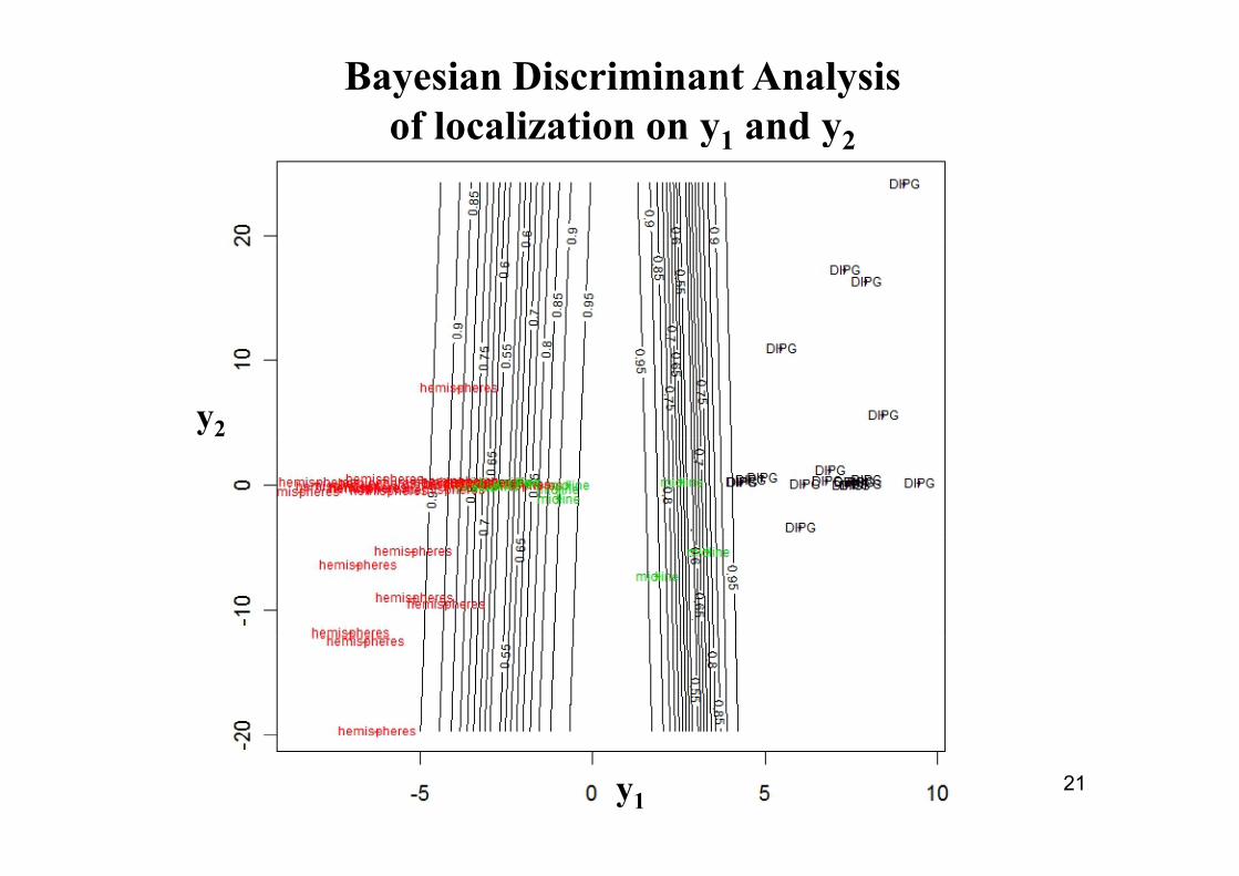
Bayesian Discriminant Analysis of localization on y1 and y2y1 y2

y2

21y1

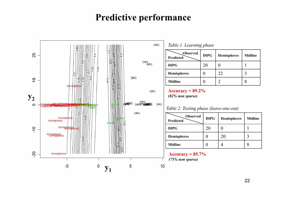
Predictive performance

Observed DIPG Hemispheres Midline

Table 1. Learning phase

Predicted DIPG Hemispheres Midline


Accuracy = 89.2% (82% non sparse)y2

ObservedPredicted DIPG Hemispheres Midline

Table 2. Testing phase (leave-one-out)


Accuracy = 85.7%(75% non sparse)

y1

22

y1

Conclusion and perspectives

• Depending on the dimension of the blocks, you can use either h i l h d l l i hthe primal or the dual algorithm.

• The dual representation of the RGCCA algorithm allows:The dual representation of the RGCCA algorithm allows:• dealing with symbolic data • recovering nonlinear relationship between blocksg p

• Sparse constraints are useful when the relevant variables are k d b (t ) i i blmasked by (too many) noisy variables.

• Sparse constraints are useful when we want to select a smallSparse constraints are useful when we want to select a small number of significant variables which are active in the relationships between blocks.

23

r t d rgccarecent advances on rgcca · pls path modeling tenenhaus m., esposito vinzi v., chatelin...

Documents