DIME – FRAGILE STATESDUBAI, MAY 31 – JUNE 4

Quasi Experimental Methods I

Nethra PalaniswamyDevelopment Strategy and GovernanceInternational Food Policy Research Institute

What we know so far

Aim: We want to isolate the causal effect of our interventions on our outcomes of interest

Use rigorous evaluation methods to answer our operational questions

Randomizing the assignment to treatment is the “gold standard” methodology (simple, precise, cheap)

What if randomization is not feasible?

>> Where it makes sense, resort to non-experimental methods

When does it make sense? Can we find a plausible counterfactual? Every non-experimental method is

associated with a set of assumptions Assumptions about plausible counterfactual The stronger the assumptions, the more

doubtful our measure of the causal effect Question assumptions

▪ Are these assumptions valid?

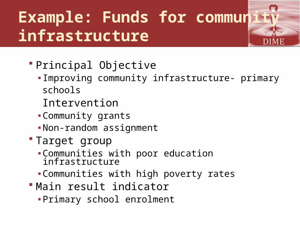
Example: Funds for community infrastructure

Principal Objective▪ Improving community infrastructure- primary

schools Intervention

▪ Community grants▪ Non-random assignment

Target group▪ Communities with poor education

infrastructure▪ Communities with high poverty rates

Main result indicator▪ Primary school enrolment

Before After0

2

4

6

8

10

12

14Control GroupTreatment Group

5

(+) Impact of the program

(+) Impact of external factors

Illustration: Funds for Community Infrastructure(1)

Before After0

2

4

6

8

10

12

14Control GroupTreatment Group

6

(+) BIASED Measure of the program impact

Before-After comparisons

Before After0

2

4

6

8

10

12

14Comparison GroupTreatment Group

7

« After » Difference betweenparticipants and non-participants

Before-After comparisons for participating and non-participating communities

« Before» Difference betweenparticipants and non-participants

>> What’s the impact of our intervention?

Difference-in-Differences Identification Strategy (1)

Counterfactual:

2 Formulations that say the same thing

1. Non-participants’ enrolments after the intervention, accounting for the “before” difference between participants/nonparticipants (the initial gap between groups)

2. Participants’ enrolments before the intervention, accounting for the “before/after” difference for nonparticipants (the influence of external factors)

1 and 2 are equivalent

Difference-in-DifferencesIdentification Strategy (2)

Underlying assumption:Without the intervention, enrolments for participants and non participants’ would have followed the same trend

>> Participating communities and non-partipating communities would have behaved in the same way on average, in the absence of the intervention

Data -- Example 1

Average enrolment

(%)2007 2008 Difference

(2008-2007)

Participants (P) 21.3 31.9 10.6

Non-participants (NP)

30.6 41.4 10.8

Difference (P-NP) -9.3 -9.5 -0.2

Data -- Example 1

Average enrolment

(%)2007 2008 Difference

(2007-2008)

Participants (P) 21.3 31.9 10.6

Non-participants (NP)

30.6 41.4 10.8

Difference (P-NP) -9.3 -9.5 -0.2

NP2008-NP2007=10.8

Impact = (P2008-P2007) -(NP2008-NP2007)

= 10.6 – 10.8 = -0.2

2007 200810

15

20

25

30

35

40

45

Participants Non-Participants

P2008-P2007=10.6

2007 200810

15

20

25

30

35

40

45

Participants Non-Participants

P-NP2008=0.5

Impact = (P-NP)2008-(P-NP)2007

= 9.3 - 9.5 = -0.2

P-NP2007=0.7

Summary

Negative Impact: Very counter-intuitive: Funding for building primary schools

should not decrease enrolment rates once external factors are accounted for!

Assumption of same trend very strong

2 sets of communities groups had, in 2007, different pre-existing characteristics and different paths

Non-participating communities would have had slower increases in enrolment in the absence of funds for building primary schools

➤ Question the underlying assumption of same trend!➤ When possible, test assumption of same trend with data

from previous years

2005 2006 2007 200810

15

20

25

30

35

40

45

ParticipantsNon-Participants

Questioning the Assumption of same trend: Use pre-pr0gram data

>> Reject counterfactual assumption of same trends !

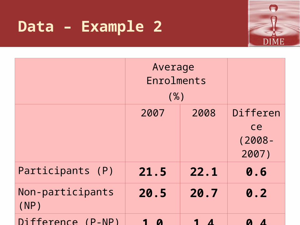
Data – Example 2

Average Enrolments

(%)2007 2008 Difference

(2008-2007)

Participants (P) 21.5 22.1 0.6

Non-participants (NP)

20.5 20.7 0.2

Difference (P-NP) 1.0 1.4 0.4

2007 200819.5

20

20.5

21

21.5

22

22.5

ParticipantsNon-Participants

P08-P07=0.6

NP08-NP07=0.2

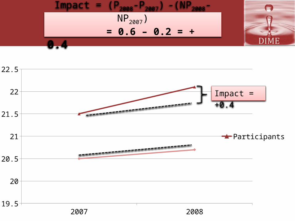
Impact = (P2008-P2007) -(NP2008-NP2007)

= 0.6 – 0.2 = + 0.4

2007 200819.5

20

20.5

21

21.5

22

22.5

ParticipantsNon-Participants

Impact = +0.4

Impact = (P2008-P2007) -(NP2008-NP2007)

= 0.6 – 0.2 = + 0.4

Conclusion

Positive Impact: More intuitive

Is the assumption of same trend reasonable?

➤ Still need to question the counterfactual assumption of same trends !➤Use data from previous years

Questioning the Assumption of same trend: Use pre-pr0gram data

>>Seems reasonable to accept counterfactual assumption of same trend ?!

2005 2006 2007 200818.5

19

19.5

20

20.5

21

21.5

22

22.5

ParticipantsNon-Participants

Caveats (1)

Assuming same trend is often problematic No data to test the assumption Even if trends are similar the previous year…

▪ Where they always similar (or are we lucky)?

▪ More importantly, will they always be similar?▪ Example: Other project intervenes in our nonparticipating communities…

Caveats (2)

What to do?

>>Check similarity in observable

characteristics

▪ If not similar along observables, chances are trends will differ in unpredictable ways

>> Still, we cannot check what we cannot see… And unobservable characteristics might matter more than observable (social cohesion, community participation)

Matching Method + Difference-in-Differences (1)

Match participants with non-participants on the basis of observable characteristics

Counterfactual: Matched comparison group

Each program participant is paired with one or more similar non-participant(s) based on observable characteristics

>> On average, participants and nonparticipants share the same observable characteristics (by construction)

Estimate the effect of our intervention by using difference-in-differences

Matching Method (2)

Underlying counterfactual assumptions

After matching, there are no differences between participants and nonparticipants in terms of unobservable characteristics

AND/OR

Unobservable characteristics do not affect the assignment to the treatment, nor the outcomes of interest

How do we do it?

Design a control group by establishing close matches in terms of observable characteristics Carefully select variables along which to

match participants to their control group So that we only retain

▪ Treatment Group: Participants that could find a match

▪ Comparison Group: Non-participants similar enough to the participants

>> We trim out a portion of our treatment group!

Implications

In most cases, we cannot match everyone Need to understand who is left out

Example

Score

NonparticipantsParticipants

MatchedIndividuals

Average incomes

Portion of treatmentgroup trimmed out

Conclusion (1)

Advantage of the matching method Does not require randomization

Conclusion (2)

Disadvantages: Underlying counterfactual assumption is

not plausible in all contexts, hard to test▪ Use common sense, be descriptive

Requires very high quality data: ▪ Need to control for all factors that influence

program placement/outcome of choice Requires significantly large sample size

to generate comparison group Cannot always match everyone…

Summary

Randomized-Controlled-Trials require minimal assumptions and procure intuitive estimates (sample means!)

Non-experimental methods require assumptions that must be carefully tested

More data-intensive Not always testable

Get creative: Mix-and-match types of methods! Address relevant questions with relevant

techniques