1

QUALITY ASSURANCE PROJECT PLAN

Assessing Sediment and Toxic Chemical Loads from the Green River, WA to the Lower Duwamish Waterway

Prepared by:

Robert Black and Kathleen Conn

U.S. Geological Survey

Washington Water Science Center

934 Broadway, Suite 300

Tacoma, WA 98402

for:

Washington State Department of Ecology

Ecology Northwest Regional Office

Toxics Cleanup Program

3190 160th Ave. SE

Bellevue, WA 98008

January 3, 2013

2

Table of Contents

Background ..........................................................................................................................4

Research Problem and Objectives .......................................................................................4

Organization and Timeline ..................................................................................................5

Data Quality Objectives .......................................................................................................7

Sampling Design ..................................................................................................................9

Field Sampling Methods ....................................................................................................14

Sample Processing .............................................................................................................18

Analytical Methods ............................................................................................................20

Quality Control Procedures................................................................................................22

Data Management, Verification, and Validation ...............................................................22

Reporting............................................................................................................................23

References ..........................................................................................................................24

Appendix A. List of analytes, methods, detection limit (DL), limit of detection (LOD), limit of quantitation (LOQ), control limits for laboratory control samples (LCS) matrix spikes (MS), as percent recovery, and control limits for laboratory replicate samples (as relative percent difference, RPD), from Analytical Resources, Inc. for water, suspended sediment, and bed sediment samples. ................................................................................26

Appendix B. List of analytes, methods, typical sample specific detection level (SDL), lower method calibration limit (LMCL), on-going precision and recovery (OPR), and replicate relative percent difference (Rep. RPD) from AXYS Analytical Services Ltd. for water, suspended sediment, and bed sediment samples. ....................................................48

3

List of Figures

Figure 1. Map of relevant locations on the Green River upstream of the Lower Duwamish Waterway Superfund Site in Seattle, WA..........................................................................11 Figure 2. Photo of the selected site, USGS 12113390 – Duwamish River at Golf Course at Tukwila, WA, located at River Mile 10.4. ........................................................12 Figure 3. Photo of example USGS sampling equipment, including a crane, reel, and sampler for representative collection of depth- and width-integrated samples. ................13 Figure 4. Flow-through centrifuge set-up (a) and centrifuge bowl (b). .............................20

List of Tables Table 1. Timeline of project tasks........................................................................................7 Table 2 (continued on next page). Summary of field collection tasks, parameters collected, collection methods, references, and laboratories completing each task. Task numbers correspond to the task numbers discussed in the text. ........................................15 Table 3. Method, sample container, minimum sediment required, preservative, and holding time of each parameter group. ..............................................................................19

4

Background

The Lower Duwamish Waterway (LDW) in Seattle, Washington is the site of intense current and historical anthropogenic influence, including numerous industrial, commercial, and residential uses. The land uses in the drainage basin include: residential (35 percent) such as the towns of South Park and Georgetown; industrial (18 percent) and commercial (11 percent) including marinas, boat manufacturing, concrete manufacturing, food processing, and airplane parts manufacturing; rights-of-way (18 percent) such as roads and highways; and open or undeveloped areas (17 percent) including parks. Decades of intense anthropogenic activities have resulted in contaminated sediments in the LDW. In 2001-2002, the U.S. Environmental Protection Agency (USEPA) and the Washington State Department of Ecology (Ecology) required remedial investigations and feasibility studies on the 5-mile, 441-acre LDW under the federal Superfund law and Washington’s Model Toxics Control Act due to concern over human health risks from exposure to contaminated sediments. The main contaminants of concern for human health include polychlorinated biphenyls (PCBs), dioxins and furans, carcinogenic polycyclic aromatic hydrocarbons (cPAHs), and arsenic. The final Feasibility Study was completed October 31, 2012, and it proposes a number of cleanup alternatives, including dredging, capping, and/or natural recovery. The draft preferred USEPA cleanup plan for the LDW is scheduled to be released for public comment in March 2013.

To support the implementation of a cleanup plan of contaminated sediments in the LDW, it is necessary to evaluate the sediment recovery potential. “Anthropogenic background” or “area background” concentrations that are higher than cleanup concentrations will result in insufficient recovery at the site. Three major sources of sediment to the LDW have been identified: upstream sources that are transported by the Green River to the LDW, lateral sources from land adjacent to the LDW, and re-suspended bed sediment within the LDW. The Sediment Transport Model (STM), developed for the LDW, predicts that every year more than 185,000 MT of sediment enters the LDW, and greater than 99 percent of that originates from upstream sources while approximately 0.5 percent originates from lateral sources and 0.2 percent originates from bed sediment within the LDW (LDWG 2008). In addition, the STM predicts that approximately 90 percent of the total bed area in the LDW receives 10 cm of new sediment within 10 years or less. Therefore, the sediment and contaminant transport and loading dynamics from the Green River to the LDW will determine, in large part, the sediment recovery potential of remediated areas in the LDW.

Research Problem and Objectives Limited field data are available regarding sediment and contaminant transport and loading dynamics from the Green River to the LDW. The STM estimated suspended and bed sediment loading into the LDW from upstream sources using grain size information and a flow-rating curve for the Green River based on discharge data from 1960-1980 and 1996-1998. That physical model was then coupled with contaminant concentration data to create a Bed Composition Model (BCM). The upstream contaminant data was extrapolated from five historic data sets from King County, Ecology, and the U.S. Army Corps of Engineers. Only one of those

5

data sets (Gries and Sloan, 2009) measured contaminants on suspended sediment (the other studies measured surface sediment or whole water). However, the sample size of the Gries and Sloan data set was relatively small (n=7) and none of the samples were collected during the rising limb of high flow events. The upstream data that were used in the BCM primarily originated from surface bed-sediment data, and it was acknowledged that those values were probably estimates of actual contaminant concentrations because the suspended sediment fraction was not fully incorporated. Typically the suspended sediment fraction is comprised of smaller particles with higher organic carbon content than surface bed-sediment particles. Hydrophobic contaminants such as PCBs and PAHs preferentially sorb to organic carbon, so it is expected that the majority of the contaminant load is transported with the fine suspended fraction of sediment. Therefore, better estimates of annual sediment loading and toxic chemical loading from suspended sediment in the Green River to the LDW are needed. The objective of this project is to quantify sediment and toxic chemical loads associated with upstream sources in the Green River to the LDW, with a focus on high flow/high turbidity events that may contribute more to the annual loading than average flow conditions. These improved measurements will aid in assessing the potential for future re-contamination of remediated sediment in the LDW.

Organization and Timeline The roles and responsibilities of key personnel involved in this project are provided in this section.

Ron Timm and Andrew Smith, Washington State Department of Ecology. Provide technical management of the project to ensure that activities are conducted in accordance with Department of Ecology guidelines and standards. Robert Black and Kathy Conn, USGS Washington Water Science Center. Implement project objectives including coordination of field sampling, processing, transport of samples for physical and chemical analysis, and data retrieval. Analyze data and provide preliminary findings to Ecology. Ensure that the project is conducted according to USGS guidelines and standards. Patrick Moran, USGS Washington Water Science Center’s Interim Water Quality Specialist. Review sampling plan and data for adherence to USGS quality assurance and control standards. Contract Laboratories and Consultants:

The USGS will contract with two Washington State accredited laboratories for analytical chemistry services and one USGS laboratory for physical sediment analysis. Coordination with these laboratories is the responsibility of the USGS and is included in the overall contract to the agency. USGS Washington Water Science Center (WaWSC) Bob Black, Supervisory Hydrologist Kathy Conn, Hydrologist

6

934 Broadway, Suite 300 Tacoma, WA 98402 Phone: (253) 552-1600 Information Officer: (253) 552-1635 Fax: (253) 552-1581 The WaWSC will be responsible for overseeing the collection, transport, shipping, payment and interpretation of all physical and chemistry data related to this project. This includes water, suspended sediment, and bed sediment samples. USGS analytical guidelines and quality parameters will be reviewed and compared for compliance and a data quality evaluation (see Wagner and others, 2007) will also be the responsibility of the WaWSC. In addition, the publication and transmittal of all final reports will be the primary responsibility of the WaWSC. USGS Cascades Volcano Observatory Sediment Laboratory (CVO) Dan Gooding, Laboratory Chief 1300 SE Cardinal Court, Building 10, Suite 100 Vancouver, WA 98683 Phone: (360) 993-8917 FAX: (360) 993-8980 dgooding@usgs.gov URL: http://vulcan.wr.usgs.gov/Projects/SedLab/framework.html The CVO will be responsible for the analysis of water samples for physical characterization of suspended sediment, including particle size distribution (PSD) and suspended sediment concentration (SSC). SSC is a measure of the amount of sediment in a given volume of water, reported as milligrams per liter (mg/L). Water samples collected using two techniques will be compared: (1) from the bridge using depth- and width-integrated techniques that ensure the sample is representative of the river’s entire cross-section (as the samples for water chemistry will be collected) and (2) from the bank using a pump from a point source (as the samples for suspended sediment chemistry will be collected). See the Field Sampling section and Table 2 for more details. Analytical Resources, Inc. (ARI) Mark Harris, Project Manager 4611 S. 134th Place Suite 100 Tukwila, WA 98168-3240 Phone: (206) 695-6200 FAX: (206) 695-6201 URL: http://www.arilabs.com/ ARI will be responsible for the analytical chemistry analysis of water, suspended sediment, and bed sediment samples for all analytes listed in Appendix A, with the exception of the dioxins, furans, and PCB congeners, which will be subcontracted to AXYS Analytical. ARI is responsible

7

for coordinating the subcontract with AXYS. ARI will provide bottles, coolers, preservatives, and chain of custody forms for each sampling event. They will provide an EPA Level 2 deliverable of all data to the USGS, which includes a summary narrative and results from all analyses (conducted at both ARI and AXYS). The data will be transmitted in two formats – one that is compatible with Ecology’s Environmental Information Management (EIM) database and one that is compatible with USGS’s National Water Information System (NWIS) database. AXYS Analytical Services LTD (AXYS) Devin Mitchell, Project Manager 2045 Mills Road Sidney BC V8L 5X2 Phone: (250) 655-5800 FAX: (250) 655-5811 URL: http://www.axysanalytical.com/ AXYS will be responsible for the analysis of water, suspended sediment, and bed sediment samples for dioxins, furans, and PCB congeners through a subcontract with ARI. They will receive samples from ARI and will provide results back to ARI that meet AXYS’ quality assurance standards. The timeline for the project is shown in Table 1.

Table 1. Timeline of project tasks.

Task Federal Fiscal Year (FY) 2013

Jan Feb Mar Apr May June

Study Design

Method Development

Field Sampling

Data Review and Analysis

Report Preparation

Data Quality Objectives

The overall data quality objective is to ensure that data of known and acceptable quality are generated. To achieve this goal, data must be reviewed for 1) precision, 2) accuracy (or bias), 3) representativeness, 4) completeness, 5) comparability, and 6) sensitivity.

8

Precision- is a measure of mutual agreement among individual measurements of the same property, under prescribed similar conditions. For this project, sampling precision from field samples will be addressed by collecting and submitting for analysis sequential replicate samples obtained during the same sampling event. One field replicate of water and one field replicate of bed sediment will be collected for chemical analysis. A field replicate will not be collected for suspended sediment because of the mass limitations. Due to the high risk of contamination by VOCs, a trip blank (a sample of deionized water filled at ARI and transported in the cooler to and from the site during field sampling) will be included in each of the five sampling events. Results from the field replicate samples will be included in the final report.

Both analytical laboratories will conduct laboratory blank, replicate, and matrix spike analyses according to their quality assurance and control plan (with every batch of approximately 20 samples). Laboratory replicates will be prepared by splitting a sample in the laboratory, and carrying the subsamples through the entire analytical process. Precision is expressed as the relative percent difference (RPD). The control limits for laboratory matrix spike and replicate samples are given in Appendix A. The replicate RPD typically is ≤ 40. The control limits for matrix spike recoveries are calculated for each individual compound. Control limits of 30 – 160 are default limits used where there is insufficient data to calculate historic control limits.

Accuracy- is a measure of the bias of a system or measurement. It is the closeness of agreement between an observed measurement value to the expected value or to the most-probable value. For this project, accuracy will be assessed through matrix spikes and continuing calibration data generated by each laboratory. When isotopes or standard reference materials are available, they will be incorporated into the sampling plan for trace organic analysis. For example, a sediment standard reference material for low-level dioxins and PCBs is available through Ecology, and will be provided to AXYS for analysis. When isotope dilution methods are available, they will be used, from which analyte concentrations are adjusted based on the extraction recovery and analytical performance of its isotope.

Representativeness- expresses the degree to which data accurately and precisely represents a characteristic of a population, parameter variations at a sampling point, a process condition, or an environmental condition. For this project, representativeness will be determined by the site selection, timing of the sampling events, sample collection methods, acceptance criteria, and sample handling and storage. To ensure samples are representative, they will be collected:

From a location in the Green River that is close to the LDW but far enough upstream to minimize potential tidal affects determined during previous studies (Embrey and Frans 2003).

During low tide conditions, to maximize collection of sediment being transported downstream from upstream sources, and minimize potential backwater tidal effects that could re-suspend and transport downstream sediment up into the sampling area.

During a range of flow conditions, focusing on high-flow events. From one or more locations within the water column at the sampling site that represents

average conditions, as determined by water quality parameters (specific conductance, turbidity, pH, dissolved oxygen), flow, and visual observations.

9

Using USGS field sampling protocols for representative samples when available and appropriate (Mueller and Wagner, 2009; U.S. Geological Survey, variously dated; Wilde and others, 2004; Davis and the Federal Interagency Sedimentation Project, 2005; Shelton 1997; Edwards and Glysson, 1999; Radke and others, 2005), as well as protocols used throughout the region (for example, Ecology, 2008).

Specifically, samples of water and suspended sediment (for physical parameters) will be flow-weighted (in other words, collected from multiple stations in the river cross-section) and depth-integrated, and will be collected using samplers (nozzles, bottles, and bags) that have been tested for non-biased sampling (the velocity through the nozzle into the sampler is the same as the velocity of the river, so as not to bias the water or sediment representation). Water samples will be composited in a Teflon churn prior to bottle filling to minimize sample variability between bottles. Bed sediment samples will be targeted from areas with a high deposition of fine sediment material in order to aptly represent the presence of fine material.

The USGS has been developing a protocol for the collection and concentration of suspended sediment using a flow-through centrifuge. For this project, suspended sediment samples collected for chemistry will initially be pumped from a point source in the river, though modifications and improvements to the sampling design may be considered during the study. See the Field Sampling section and Table 2 for more details.

Completeness- is a measure of the amount of acceptable analytical data obtained from a measurement system compared to the amount that was expected to be obtained under normal conditions. Target completeness values are 90% for chemical analyses of water and sediment.

Comparability-expresses the confidence with which one data set can be compared to another. For this project, comparability will be achieved through the use of standard EPA-approved laboratory methods. In addition, standard techniques to collect and analyze representative samples will be used. This will allow comparison to previous (for example, Gries and Sloan 2009) and ongoing (for example, ongoing USGS study on large Puget Sound rivers) data sets.

Sensitivity- is a measure of the analytical capability of the methods to meet the project objectives. The analytical limit of quantitation (LOQ) goals for ARI are presented in Appendix A. The analytical goals for AXYS, including typical sample specific detection level (SDL) and lower method calibration limit (LMCL) are presented in Appendix B. The contract analytical laboratories were specifically selected because of their ability to detect analytes at low level concentrations (for example, ng/L and less). In addition, one water sample field blank will be collected for chemical analysis. An equipment-blank associated with the five suspended sediment samples will be tested by passing a slurry of clean sediment and deionized water through entire sampling set up including the pump tubing, Teflon-lined bucket, peristaltic pump setup, and centrifuge. Results from the field and equipment blanks will indicate if the equipment cleaning, sampling collection, handling, and processing procedures introduce contamination that could increase the low reporting level.

Sampling Design

10

Approach: Between January and June 2013, the USGS Washington Water Science Center will collect representative samples of water, suspended sediment, and bed sediment from a single strategically-located site on the Green River, WA during five hydrologic events ranging in flow conditions. Samples will be analyzed by Washington State-accredited laboratories for a large suite of compounds, including PAHs and other semivolatile compounds, PCB aroclors and the full suite of 209 congeners, volatile compounds, metals including arsenic, dioxins and furans, pesticides, tributyltin, and total organic carbon. Concurrent with the chemistry sampling, we will measure SSC and PSD. From these and already available stream flow data, we will calculate preliminary estimates of toxic chemical loads from the Green River to the Lower Duwamish Waterway.

Site Description: The lower Duwamish/Green River basin is nearly flat and the tidal influence extends year-round more than 12 miles upstream from the river mouth (Figure 1, “D”) and during low-flow conditions at least 17 miles upstream (Figure 1, “G”). Sampling at a location upstream of tidal influence will not capture effects from all potential sources upstream of the LDW. However, sampling near the upstream boundary of the LDW (River Mile, RM, 5) will be in estuarine conditions with very strong tidal influences. Because the primary goal of this project is to assess toxic loads on suspended sediment originating from upstream sources, it is of singular importance to select a site where sampling protocols can be modified to minimize collection of suspended sediment that originates from the LDW and has been re-suspended and transported upstream during high tides.

The single sampling location selected is USGS 12113390 – Duwamish River at Golf Course at Tukwila, WA (Figure 1, “C” and Figure 2). The site is located at approximately RM 10.4. Between 1995 and 2004, samples were collected approximately monthly at this site as part of the USGS National Water Quality Assessment (NAWQA) program. Discharge, specific conductance, nutrients, metals, pesticides and organics in water and a limited number of bed sediment samples were measured. Instantaneous discharge values ranged from 230 to 13,200 cubic feet per second (cfs), with a median value of 1390 cfs (n=116). The highest measured instantaneous discharges were recorded during large storm events in the late winter season (January through April) in 1996 and 1997 (note that this is an instantaneous, not continuous, discharge record). Elevated SSC values were often measured concurrently with elevated discharge. SSC ranged from 3 to 787 mg/L (n=114), with a median value of 19 mg/L. During all NAWQA sampling events, which were targeted during low tide conditions, specific conductance values were less than 200 S/cm, suggesting that the salinity influence at this site is negligible. The cross section promotes good mixing of the water column as the bridge supports are on the bank and there are no large bridge abutments or other disruptions to flow and mixing in the water (Figure 2). In addition, the site location provides safe sampling access because it is a wide bridge with limited golf cart and foot traffic only. After hours, the bridge can only be accessed through a locked gate (for which the USGS has a key), providing heightened security compared to other sites.

11

Figure 1. Map of relevant locations on the Green River upstream of the Lower Duwamish Waterway Superfund Site in Seattle, WA.

A: Approximate upstream boundary of the Lower Duwamish Waterway Sediment Cleanup Site (River Mile, RM, 5)

B: Ecology Location Name LDWRRUN0 (RM 6.7); location of previous suspended sediment sampling (Gries and Sloan 2009)

C: USGS 12113390 – Duwamish River at Golf Course at Tukwila, WA; site of historic NAWQA sampling and selected sampling location for this study (RM 10.4)

D: USGS 12113350 – Green River at Tukwila, WA; stage-only gage (RM 12.4)

E: USGS 12113346 – discharge gage accounting for Springbrook Creek input to Green River

F: USGS 12113349 – discharge gage accounting for Mill Creek input to Green River

G: USGS 12113344 – Green River at 200th Street at Kent, WA; discharge gage, flow rating is under development (RM 17)

12

Figure 2. Photo of the selected site, USGS 12113390 – Duwamish River at Golf Course at Tukwila, WA, located at River Mile 10.4.

We considered the site of the previous suspended sediment investigation (Gries and Sloan, 2009) - Ecology Location Name LDWRRUN0 (RM 6.7). This site is approximately 3 to 4 miles closer to the upstream boundary of the LDW (Figure 1, “B”); however, it is located in more estuarine conditions. During the previous study, the salinity gradient was often present, with salinity values around 20 ppt at the bottom of the water column and occasionally exceeding 3 ppt (a common freshwater/saltwater threshold) at the mid-column sampling point during August sampling events (Gries and Sloan, 2009, Appendix D). The vertical bridge supports have large wood abutments extending into the water, increasing the difficulty in obtaining a well-mixed, representative sample of the cross-section. Also, the footbridge is accessible by the public 24 hours a day, increasing safety concerns and limiting the ability to effectively use appropriate USGS equipment including a bridge crane, reel, and sampler (Figure 3).

13

Figure 3. Photo of example USGS sampling equipment, including a crane, reel, and sampler for representative collection of depth- and width-integrated samples.

Development along the river between the USGS site (RM 10.4) and the Ecology site (RM 6.7) includes the golf course, a small commercial complex, and residential properties. The contaminant contributions to the river from this reach are expected to be minimal, primarily consisting of stormwater outfalls. The sampling design will include a comparison of samples collected at both sites for water quality parameters such as SSC, PSD, specific conductance, and turbidity to assess data comparability between sites.

The selected USGS site meets the criteria of: (1) capturing and representing the majority of upstream sources to the LDW while minimizing tidal influence, (2) providing data that can be compared to historic data, and (3) providing safe sampling access using appropriate equipment.

Real-time stage and discharge measurements from nearby upstream stations will be used to inform sampling. This includes the following stations (Figure 1, “D”, “E”, “F”, and “G”, respectively): 12113350 (Green River at Tukwila, WA, RM 12.4, stage only due to tidal influence), 12113346 (Springbrook discharge contribution, typically <2%), 12113349 (Mill Creek discharge contribution, typically less than 5%), and 12113344 (Green River at 200th Street in Kent, WA, RM 17, discharge rating under development, low-flow tidal influence). A minimum stage threshold of 10 ft. at USGS 12113350 (Green River at Tukwila, WA) is ideal,

14

which would have resulted in 5 sampling events between January 1 and June 30, 2012. Sampling events may occur during lower flow conditions so as not to bias the results. In addition, a conductivity data logger and pressure transducer to monitor river stage will be installed onsite at the sampling location over the duration of the project. We will use the conductivity information and the continuous river stage data at the site to calibrate flow and stage data from upstream sources to assess the tidal influence at the site. Based on historic data, we expect the tidal influence to be variable backwater conditions during most times of the year. To minimize tidal backwater effects (that could transport sediment upstream), samples will be collected during a 6-hour window surrounding low tide.

Field Sampling Methods

During each of the five proposed sampling events, six tasks will occur to measure the following parameters: 1) instantaneous discharge, 2) general water quality, 3) water chemistry, 4) suspended sediment physical parameters, 5) suspended sediment chemistry, and 6) bed sediment chemistry. A summary of these tasks is contained in Table 2 and a more detailed description is provided below.

Task 1) Instantaneous discharge. Discharge will be measured using an acoustic Doppler current profiler (ADCP) following standard USGS protocols (Mueller and Wagner, 2009).

Task 2) General water quality. Water quality parameters including water temperature, pH, dissolved oxygen, specific conductance, and turbidity will be measured using a multiparameter sonde (YSI Inc., Yellow Springs, OH) and/or other hand-held devices such as the Analite turbidity sensor (McVan Instruments, Victoria, Australia).

Task 3) Water chemistry. Based on the discharge measurements and stream width, the river cross-section will be divided into equal discharge increments (EDI) or equal width increments (EWI) for water chemistry analysis and suspended sediment physical parameter analysis (see Task 4) using standard USGS protocols (U.S. Geological Survey, variously dated) including those specific for sampling of trace organic chemicals (Wilde and others, 2004). This sampling technique collects a depth- and width-integrated isokinetic sample that is representative of the entire river cross-section at that sampling site. Briefly, a sampler is lowered at a consistent transit rate from the surface to the bottom and back to the surface of the water column at each station. The process is repeated as necessary to obtain sufficient sample. Water samples will be collected from each cross-section station in Teflon bottles or bags using an approved sampler, such as the D-96 (Davis and the Federal Interagency Sedimentation Project, 2005). The water samples will be composited in a 14-L Teflon churn and immediately processed in an on-site mobile laboratory (see Sample Processing). Volatile organic compounds (VOCs) will be collected separately using a USGS tested and designed hand-held sampler to avoid losses due to sample pouring, transferring, and churning (Shelton 1997). The sampler, containing four 40 mL glass vials will be lowered to a mid-point in the vertical water column at a single station in the centroid of flow. Water fills the bottles slowly from the bottom to avoid turbulence and head space that could results in analyte losses. A complete list of analytes being characterized in all water samples is contained in Appendix A and B.

15

Table 2 (continued on next page). Summary of field collection tasks, parameters collected, collection methods, references, and laboratories completing each task. Task numbers correspond to the task numbers discussed in the text.

Task No.

Task Description Parameter Collected Collection Method

Published Collection Methods Laboratory Notes

1 Instantaneous discharge

River discharge (ft3/sec) Acoustic Doppler Current Profiler (ADCP)

Muller and Wagner, 2009.

USGS-Tacoma

-

2 General water quality (field parameters)

Water temperature (⁰C), pH, dissolved oxygen (mg/L), specific conductance (µS/cm), turbidity (NTU)

Teledyne YSI multiparameter sonde; Analite turbidity sensor

USGS National Field Manual for the Collection of Water-Quality Data (NFM), variously dated.

USGS-Tacoma

-

3 Water chemistry

Dioxins, Furans, PCB Aroclors and 209 congeners, Semivolatile Compounds, PAHs, Pesticides, Tributyl tin, Trace Elements (metals) including mercury and hexavalent chromium, total organic carbon. See Appendix A and B for complete list of analytes.

Depth- and width-integrated isokinetic sample representative of entire river cross-section using Teflon samplers. Sample transferred to Teflon churn in on-site mobile lab for complete homogenization prior to sample processing.

Wilde and others, 2004; Davis and the Federal Interagency Sedimentation Project, 2005; USGS NFM, variously dated.

Analytical Resources, Inc. (ARI), Tukwila, WA and AXYS Analytical Services LTD (AXYS), British Columbia, Can.

-

3 Water chemistry (VOCs)

Volatile Organic Compounds (VOCs) (µg/l). See Appendix A and B for complete list of analytes.

USGS hand-held VOC sampler designed to minimize chemical loss. Sample collected at 60% of depth at the centroid of flow.

Shelton, 1997. ARI -

4 Suspended sediment physical parameters

Characterization of abundance of suspended sediment in a volume of water, expressed as suspended sediment concentration (SSC, mg/L). Characterization of size distribution of suspended sediment particles, expressed as a particle size distribution (PSD).

Depth- and width-integrated isokinetic sample representative of entire river cross-section. This cross-section sample will be collected immediately after the water chemistry cross-section sample using USGS suspended sediment sampling protocol.

Edwards and Glysson, 1999; Radke and others, 2005.

USGS Cascades Volcano Observatory Sediment Laboratory (CVO), Vancouver, WA

No chemical analyses will be conducted on these samples. Results will be interpreted with the suspended sediment chemistry sampling results (Task 5) to assess potential load of suspended sediment-bound chemicals.

16

Table 2 (continued from previous page). Summary of field collection tasks, parameters collected, collection methods, references, and laboratories completing each task. Task numbers correspond to the task numbers discussed in the text.

Task No.

Task Description Parameter Collected Collection Method

Published Collection Methods Laboratory Notes

5 Suspended sediment chemistry

Dioxins, Furans, PCB Aroclors and 209 congeners, Semivolatile Compounds, PAHs, Pesticides, Tributyl tin, Trace Elements (metals) including mercury and hexavalent chromium, VOCs, total organic carbon. See Appendix A and B for complete list of analytes.

Concurrent with water chemistry sampling, 1000-2000 liters of sediment-laden river water will be pumped at 60% of depth at centroid of flow through a Teflon tube into Teflon-lined buckets. Suspended sediment will be separated the from water by flow-through centrifuge for chemical analysis.

Sample collection methods developed as part of this project. Sediment handling methods: Shelton and Capel, 1994.

ARI and AXYS

An additional 5-10 liters of water will be pumped to compare SSC and PSD in the pumped sample to SSC and PSD in the depth- and width-integrated sample (Task 4). Also, the centrifuge effluent water will be analyzed for SSC and PSD to determine efficiency rates and the size distribution of un-captured sediment.

6 Bed sediment chemistry

Dioxins, Furans, PCB Aroclors and 209 congeners, Semivolatile Compounds, PAHs, Pesticides, Tributyl tin, Trace Elements (metals) including mercury and hexavalent chromium, VOCs, total organic carbon. See Appendix A and B for complete list of analytes. Also grain size.

The top 10 cm of sediment from a minimum of 10 depositional areas containing fine-grained particles located within 1000 m up- or down-stream of site will be collected and composited with Teflon and glass sampling equipment. All samples sieved to <2 mm. Trace element and mercury samples sieved with nylon sieve. Organic samples sieved with stainless steel sieve.

Radke and others, 2005; Shelton and Capel, 1994; Ecology, 2008.

ARI and AXYS

If excess sediment is collected, additional sample may be wet sieved through a 63 m sieve to assess differences in sediment chemistry between the fine fraction (<63 m) and the sand fraction (63 m < x < 2mm).

17

Task 4) Suspended sediment physical parameters. After completing one cross-section of depth- and width-integrated isokinetic sampling for water chemistry, a second cross-section of depth- and width-integrated isokinetic sampling will be completed to characterize the abundance and size distribution of suspended sediment using standard USGS protocols (Edwards and Glysson 1999, Radke and others, 2005). Again, approved samplers, nozzles, bags, and bottles will be used. The volume of water collected will depend on current sediment conditions, and is expected to range between 5 and 50 L. The samples will be stored until transport to CVO for analysis of SSC and PSD. These samples will not receive any chemical analyses, but will be used to characterize the abundance and size distribution of suspended sediment at the time of concurrent suspended sediment chemistry sampling (see below). An accurate representation of the abundance and size distribution of suspended sediment will be combined with the suspended sediment chemistry sampling results (see Task 5) to help assess the potential load of suspended sediment-bound chemicals being transported downstream.

Task 5) Suspended sediment chemistry. Concurrent with tasks 3) and 4), a separate team will pump river water from a point source through Teflon tubing into sequential 5-gallon buckets lined with Teflon bags for suspended sediment chemistry analysis. An ISCO pump (Teledyne ISCO, Lincoln, Nebraska) or similar non-screened, high-flow pumping device will be used. The point-sampling location will be located at a depth approximately 0.6 times the main channel depth in a section favoring fine particulates as determined based on ADCP data during each sampling trip. The volume of water collected will depend on the current river turbidity and sediment conditions, and will likely be between 1000 and 2000 liters (50 to 100 5-gallon buckets). The sample-filled Teflon bags will be closed, sealed in their bucket, labeled, and transported to the Washington Water Science Center for concentration of suspended sediment using flow-through centrifuges (see Sample Processing). Sediment collected from the centrifuge will be analyzed for those compounds listed in Appendix A and B. A sample of pumped water will also be collected into a large container for analysis of SSC and PSD at CVO to compare to the results from the representative samples collected in Task 4. During low-flow/low-turbidity sampling events, a follow-up site visit to collect additional water for centrifugation may be necessary, and will occur during the next feasible low tide condition.

Task 6) Bed sediment chemistry. A bed sediment sample will be collected during five non-storm events, which may occur on the same day as Tasks 1 - 5 or during lower flow conditions preceding or succeeding the other sampling activities. Samples will be collected according to Ecology and USGS protocols (Ecology, 2008; Radke and others, 2005; Shelton and Capel, 1994) for the same suite of chemical parameters as the suspended sediment samples (Appendix A and B) and grain size analysis. Depending on the conditions, the samples will be collected from the bridge, bank, or boat. Samples (0-10 cm depth) from multiple locations near the site will be composited into a single sample. Locations will be selected to focus on areas with a high deposition of fine material. The composited sample immediately will be processed in an on-site mobile laboratory (see Sample Processing).

18

Sample Processing Dissolved Water Chemistry Sample Processing (see Task 3 above) In the mobile laboratory, the composited water sample will be churned according to USGS protocols (U.S. Geological Survey, variously dated) to ensure sample homogenization prior to bottle filling. Pre-acidified bottles will be used for samples requiring preservation (See Table 3). Labels will be completed and samples will be stored on ice until transportation within 6 hours to ARI for analysis. Suspended Sediment Chemistry Sample Processing (see Task 5 above) At the Washington Water Science Center Field Services Unit located in Tacoma, WA, water from the 5-gallon Teflon bags will be pumped into a continuous flow-through centrifuge (CFC Express, Scientific Methods, Inc., Granger, IN) to concentrate the suspended sediment (Figure 4). The centrifuge runs at a fixed speed of 10,000 revolutions per minute, and preliminary testing suggests that the inflow rate be no more than 300 mL/min to ensure sediment capture efficiencies greater than 90 % (by weight). Water samples will be pumped from the buckets using Teflon tubing, C-FLEX, and a peristaltic pump into the centrifuge. At a flow rate of 300 mL/min, approximately one bucket per hour can be centrifuged. With two flow-through centrifuge units running in parallel, approximately 25 to 50 hours of centrifugation will be required for each sampling event. Pre-centrifuged water in buckets will be kept at 4 °C until centrifugation. Periodically, concentrated sediment from the centrifuge bowl will be composited in a pre-tared glass jar and stored quiescently at 4 °C. Excess overlying water will be decanted by pipette. The total wet weight of the sediment will be recorded. In addition, SSC of centrifuge influent and effluent will be compared to determine sediment capture efficiency. Finally, the PSD of un-captured sediment in the centrifuge effluent will be determined during each sampling event. If sufficient suspended sediment is collected exceeding the mass requirements for the methods listed in Table 3 (approximately 100-150 g), a subset of the sediment sample will be separated by size fraction (sand and fine) by wet sieving. Using a 63 m Viton mesh supported by a Teflon ring, the sediment will be wet sieved into a fines fraction (<63 m) and a sand fraction (63 m to 2 mm). Each size fraction will be sent to ARI for chemical analysis (see Analytical Methods section below). Contaminant concentrations associated with each size fraction will be compared to results from the whole (un-sieved) sediment sample to assess the proportion of contaminants associated with each size fraction. This information may inform the analytical scheme for future projects regarding the need to analyze all size fractions or focus on one size fraction, such as the fines less than 63 m in diameter.

19

Table 3. Method, sample container, minimum sediment required, preservative, and holding time of each parameter group.

Analytical Parameter EPA

Method Sample Container Min. Sed. Required

(dry weight)

Preservative Holding Time

Water Sediment Water Sediment

Dioxins, Furans, and 209 PCB congeners 1613/1668 2 x 500 mL AG 8 oz. WMG

(amber) 10 g Cool ≤ 6 °C 7 d 14 d

Semivolatile Compounds 8270D 2 x 500 mL AG 8 oz. WMG 15 g Cool ≤ 6 °C 7 d 14 d Polycyclic Aromatic Hydrocarbons (PAHs)

8270-SIM LL 2 x 500 mL AG 8 oz. WMG 15 g Cool ≤ 6 °C 7 d 14 d

Polychlorinated biphenyls (PCBs) 8082 LL 2 x 500 mL AG 8 oz. WMG 15 g Cool ≤ 6 °C 7 d 14 d Pesticides 8081 2 x 500 mL AG 8 oz. WMG 15 g Cool ≤ 6 °C 7 d 14 d Tributyl tin Krone 2 x 500 mL AG 8 oz. WMG 5 g Cool ≤ 6 °C 7 d 14 d Trace Elements (metals) 200.8 500 mL HDPE 4 oz. WMG 2 g 2.5 mL 1:1 HNO31 6 mo 6 mo Mercury 7470-LL 500 mL HDPE 4 oz. WMG 2 g 5 mL 1:1 HNO31 28 d 28 d Hexavalent Chromium 7196 500 mL HDPE 4 oz. WMG 5 g Cool ≤ 6 °C 24 hr 28 d

Volatile Organic Compounds 8260 3 x 40 mL vial, no headspace

2 oz. WMGS (no headspace) 5 g Cool ≤ 6 °C 7 d 14 d

Total organic carbon 415.1 250 mL AG - - Cool ≤ 6 °C + pH <2 w/ 2mL H2SO4 28 d -

Total organic carbon Plumb 1981 - 4 oz. WMG 1 g Cool ≤ 4 °C - 14 d Total solids - 4 oz. WMG 5 g Cool ≤ 6 °C - 14 d Grain size PSEP - 16 oz. WMP 50 g Cool ≤ 6 °C - 14 d

1 Preservation for water samples only AG = amber glass Boston round bottle HDPE = high-density polypropylene WMG = wide-mouth glass jar WMGS = wide-mouth glass jar with septa

20

Figure 4. Flow-through centrifuge set-up (a) and centrifuge bowl (b).

Bed Sediment Chemistry Sample Processing (see Task 6 above) The bed sediment sample will be composited and homogenized using a Teflon spatula in the mobile laboratory immediately after sample collection. All sediment will be wet sieved through a 2 mm diameter sieve prior to jar filling. Samples for metals analysis will be processed through a plastic sieve (cleaned in soap, water, dilute hydrochloric acid, and methanol), and samples for all other analyses will be processed through a stainless steel sieve (cleaned in soap, water, and methanol). Similar to the suspended sediment processing described in the previous paragraph, if sufficient bed sediment is collected, a wet sieving technique will be tested to separate the sample into a fines fraction (<63 m) and a sand fraction (63 m to 2 mm) for analysis. Standard USGS protocol (Shelton and Capel 1994) describes analysis of organic compounds on sediment <2 mm in diameter, and analysis of trace elements on sediment <63 m in diameter. We will test the feasibility of applying this protocol to the current site during the first bed sediment sampling events.

Analytical Methods Samples of water (Task 3), suspended sediment (Task 5), and bed sediment (Task 6) will be analyzed for a suite of over 200 chemical parameters (Appendix A), TOC, and total solids and grain size (sediment samples only) at ARI. ARI is a Washington State-accredited laboratory providing low-level organic and inorganic analyses. The parameters groups and EPA Method are listed in Table 3. Found in Appendix A, for both water and sediment, are all the ARI analytes listed individually with the following information:

EPA Method number, Detection Limit (DL) – the lowest result that can be reliably distinguished from a blank with a false

positive rate ≤ 1%, Limit of Detection (LOD) - the lowest result that can be reliably distinguished from a blank based on

historical method blank detections, according to NELAP certification requirements, Expected Limit of Quantitation (LOQ) – the smallest detectable concentration of analyte greater than the

LOD that meets specific criteria with respect to precision and accuracy based upon method performance of samples spiked at or near the LOQ with a false negative rate ≤ 5%,

Control limits for laboratory matrix spikes (as percent recovery), and

21

Control limits for laboratory replicates (as RPD). ARI’s results will be reported to the LOQ with J-flagging down to the LOD. ARI’s Quality Assurance Plan, which includes information such as continuing calibration data for each method, can be found at: http://www.arilabs.com/portal/index.php?option=com_remository&Itemid=51&func=fileinfo&parent=category&filecatid=16. ARI’s Data Reporting Qualifiers can be found at: http://www.arilabs.com/portal/index.php?option=com_remository&Itemid=51&func=fileinfo&parent=category&filecatid=87. In addition, samples will be analyzed for dioxins, furans, and the full suite of 209 PCB congeners through a subcontract to AXYS Analytical Services Ltd. (AXYS), located in British Columbia, Canada (http://www.axysanalytical.com/). AXYS also is a Washington State-accredited laboratory specializing in ultra-trace analysis of persistent organic pollutants and emerging contaminants. Found in Appendix B, for both water and sediment, are the AXYS analytes listed individually with the following information:

EPA Method number, Typical Sample-specific Detection Limit (SDL) – the concentration equivalent to 3 times the estimated

chromatographic noise height, determined individually for every sample analysis run, Lower Method Calibration Limit (LMCL) – determined by prorating the concentration of the lowest

calibration limit for sample size and extract volume. The following equation is used: ((lowest level calibration standard) x (extract volume))/sample size,

On-going precision and recovery (OPR) for laboratory matrix spikes (as percent recovery), and Control limits for replicates (as RPD).

AXYS results will be reported to the LMCL and J-flagged down to the SDL, as consistent with standard State of Washington protocols. A minimum of 100 to 150 g of sediment is required to complete the chemical analyses. During low-turbidity sampling events, even with consecutive days of water collection, there may be insufficient sediment concentrated from the centrifuge to complete all 11 methods. In these cases, a priority list of analytical methods will be followed (with #1 being the top priority):

1. Total solids (always completed; needed to report a dry weight concentration) 2. Total organic carbon 3. Dioxins/Furans/PCB Congeners (a single co-extraction by AXYS) 4. PCB Aroclors 5. PAHs 6. Metals (including mercury) 7. Semivolatile compounds 8. Pesticides 9. Hexavalent Chromium 10. Tributyl tin 11. Volatile organic compounds

The VOCs are the lowest priority because, based on their volatility and the turbulent sampling techniques (pumping and centrifuging), analyte losses during sediment collection are likely. All efforts will be made to collect

22

sufficient sediment to complete all 11 methods, and it is expected that there will be sufficient sediment to analyze the priority methods (#1-6) in all situations.

Quality Control Procedures USGS quality assurance procedures for surface-water measurements and water-quality sampling and analysis will be followed (Wagner and others, 2007; U.S. Geological Survey, variously dated). This includes the proper equipment selection, cleaning procedures, and sampling protocols for low level organic compounds, VOCs, and metals. Sampling equipment for chemical analyses will be Teflon and will be pre-cleaned with phosphate-free soap, rinsed three times with tap water, soaked in 5% hydrochloric acid, rinsed with deionized water, rinsed with high purity methanol, and air dried. Field sampling techniques include various measures to avoid sample contamination including the “clean hands, dirty hands” technique and processing of water samples in a clean mobile laboratory. Hydrologists and hydrological technicians on this project have been trained at the National Training Center in the collection of water quality samples, including samples for trace organic and low level mercury analyses. The field folder will include copies of the QAPP and the protocols referenced within. Deviations from the QAPP will be noted on the field sheet. Detections of parameters above the reporting level in the field and/or equipment blank indicate the introduction of contamination during the cleaning, sampling, handling, and processing of the environmental samples. Data will be qualified as described in the USGS Office of Water Quality Technical Memorandum 2012.01 (http://water.usgs.gov/admin/memo/QW/) which states that detections less than 3 times the blank concentration be given a “<” qualifier (“less than” the detected concentration) while detections between 3 and 10 times the blank concentration be given an “E” code (for “estimated”). Detections greater than 10 times the blank concentration will not be qualified. The water and bed sediment field replicates will be reviewed as an indication of field variability. Results from laboratory quality assurance samples (a blank, replicate, and matrix spike per batch of 20 samples) will be reviewed by laboratory personnel. If values exceed control limits (Appendix A and B) then laboratory personnel will take appropriate corrective actions such as re-runs and re-extractions and/or discuss modifications to the protocol with the principal investigator.

While both analytical laboratories (ARI and AXYS) are State-accredited, they are not associated with the USGS’s National Water Quality Laboratory and do not perform the same QA/QC procedures necessary to permit immediate inclusion in the USGS’s national and publically accessible database. Therefore, some additional project resources will be used to perform the necessary quality assurance examination of the data that will allow the USGS to include the results in its database. A Laboratory Evaluation Program (LEP) will be conducted by project personnel according to the guidance provided by the USGS Branch of Quality Systems (http://devbqs.cr.usgs.gov/LEP/index.php) and in accordance with USGS Office of Water Quality Technical Memorandum 2007.01.

Data Management, Verification, and Validation A field form, modified from the standard USGS Surface Water Quality Notes, will be completed during each sampling event. Field parameters recorded will include date, time, sampling team, field conditions, sampler types, sampling methods, meter and probe serial numbers and calibration information, number and type of quality assurance samples collected, and any deviations from the sampling protocol.

23

Field parameters, including water temperature, specific conductance, dissolved oxygen, pH, and turbidity will be compiled on the field form and reviewed by one of the USGS principal investigators prior to entry into the USGS National Water Information System (NWIS). The instantaneous discharge record during each sampling event will be worked up according to standard USGS protocols (Mueller and Wagner, 2009), which includes verification and validation by secondary and tertiary reviewers, prior to entry into NWIS. Quality-assurance procedures used by the Washington Water Science Center for activities related to the collection, processing, storage, analysis, and publication of surface-water data are described in detail by Kresch and Tomlinson (2004). Quality assurance procedures utilized by USGS sediment laboratories for analysis of suspended-sediment concentration are provided by Knott and others (1992; 1993) and Matthes and others (1992). Prior to sending samples to the laboratory, analytical services requests for determination of suspended-sediment concentration and particle-size analysis and sample site and other information are entered into the Sediment Laboratory Environmental Data System (SLEDS). The laboratory results are also entered into the system. Documentation of SLEDS is available online at http://eris.wr.usgs.gov/SedLab/framework.html. All analytical results from AXYS and ARI will be compiled and transmitted to the USGS Washington Water Science Center. The Level 2 deliverable includes a hard-copy written narrative and tables of results including quality assurance information. The data will also be delivered electronically in two formats – one that is compatible for entry into Ecology’s Environmental Information Management (EIM) database and one that is compatible for entry into USGS’s NWIS. New parameter codes and/or method codes specific to this project will be requested as necessary for the water quality database of NWIS. All data, including the field parameters, physical sediment results, and analytical chemistry results, will be reviewed and validated by Washington Water Science Center project personnel, equivalent to an EPA Level 3 data package. Subsequently, the Center’s Water Quality Specialist will review the data as a 3rd-party independent reviewer, comparable to an EPA Level 4 data package. Data qualifiers or flags may be applied to data by either laboratory or project personnel pending review of quality assurance data and the Center’s Water Quality Specialist. Common data qualifiers include, but are not limited to: B Analyte detected in method blank J Estimated concentration is less than established reporting limits E Estimated concentration above the valid instrument calibration range Data that has been flagged or qualified by the laboratory or during the USGS review process will be reported as measured with the qualifier, unless an alternative reporting method is deemed necessary. The USGS review process follows the USGS’ Fundamental Science Practices (http://www.usgs.gov/fsp/default.asp) to provide unbiased, objective, and impartial scientific information. Reviewed data will be entered into both Ecology and USGS database systems for long-term storage and access.

Reporting Tidal exchange information at the site (for example, discrete measurements of stage, discharge, and SSC compared to nearby continuous measurements of stage and discharge) will be combined with chemistry data to determine preliminary estimates of net downstream loading of sediment, sediment-bound contaminants, and dissolved contaminants. A draft of the data report, in the form of a USGS Data Series Publication, will be prepared with the available data in early summer 2013 and submitted to Ecology by June 30, 2013. The draft will contain tables of concentration results for all analytes and other parameters in water, suspended sediment, and bed sediment for each of the five sampling events. The concentrations will be compared to published criteria, when

24

available. Preliminary loading calculations will be presented based on discharge and dissolved concentrations (for dissolved loading) and discharge, SSC, and particulate-bound contaminants (for particulate-bound loading). For analytes that are not detected during the study, a loading calculation will be calculated based on the reporting limit and reported as “less than” the calculated value. For analytes that are detected during some, but not all, sampling events, a value of one half of the reporting level will be used for the non-detects to calculate the loading, and the data will be qualified. The results from this 5-month study will provide preliminary information about the types of toxic chemicals that have the potential to reach the LDW from the Green River, and will inform future investigations for improving these loading estimates.

References Davis, B.E.; Federal Interagency Sedimentation Project, 2005, A guide to the proper selection and use of federal

approved sediment and water-quality samplers: USGS Open-File Report 2005-1087, 26 p., accessed February 1, 2013 at http://pubs.usgs.gov/of/2005/1087/.

Ecology, 2008., Sediment Sampling and Analysis Plan Appendix. Toxics Cleanup Program, Washington State

Department of Ecology, Publication No. 03-09-043, accessed December 4, 2012 at https://fortress.wa.gov/ecy/publications/summarypages/0309043.html.

Edwards, T.K. and Glysson, G.D., 1999, Field Methods for Measurement of Fluvial Sediment: Techniques of Water-Resources Investigations of the U.S. Geological Survey, book 3, chap. C2, accessed December 4, 2012 at http://pubs.usgs.gov/twri/twri3-c2/html/pdf.html.

Embrey, S.S., and Frans, L.M., 2003. Surface-Water Quality of the Skokimish, Nooksack, and Green-Duwamish Rivers and Thornton Creek, Puget Sound Basin, Washington, 1995-98: USGS Water-Resources Investigations Report 2002-4190, accessed March 8, 2013 at http://pubs.er.usgs.gov/publication/wri024190.

Gries, T. and Sloan, J., 2009. Contaminant Loading to the Lower Duwamish Waterway from Suspended Sediment in the Green River. Environmental Assessment Program, Washington State Department of Ecology. Report Number 09-03-028, accessed December 4, 2012 at https://fortress.wa.gov/ecy/publications/summarypages/0903028.html.

Knott, J.M., Glysson, G.D., Malo, B.A., and Schroeder, L.J., 1993, Quality Assurance Plan for the Collection and Processing of Sediment Data by the U.S. Geological Survey, Water Resources Division: U.S. Geological Survey Open-File Report 92-499, accessed January 3, 2013 at http://pubs.er.usgs.gov/pubs/ofr/ofr92499.

Knott, J.M., Sholar, C.J., Matthes, W.J., 1992, Quality Assurance Guidelines for the Analyses of Sediment Concentration by U.S. Geological Survey Sediment Laboratories: U.S. Geological Survey Open-File Report 92-33, accessed January 3, 2013 at http://pubs.er.usgs.gov/pubs/ofr/ofr9233.

Kresch, D.L., and Tomlinson, S.A., 2004, Surface–Water Quality–Assurance Plan for the U.S. Geological Survey Washington Water Science Center: U.S. Geological Survey Open-File Report 03-490, 50 p.

Lower Duwamish Waterway Group (LDWG), 2008. Lower Duwamish Waterway Sediment Transport Modeling Report Final. Prepared for U.S. Environmental Protection Agency (Region 10 - Seattle, WA) and Washington State Department of Ecology (Northwest Regional Office, Bellevue, WA). Prepared by Quantitative Environmental Analysis, LLC Montvale, NJ. Accessed December 4, 2012 at www.ldwg.org/rifs_docs4.htm#stm.

25

Matthes, W.J., Sholar, C.J., George, J.R., 1992, Quality-Assurance Plan for the Analysis of Fluvial Sediment by Laboratories of the U.S. Geological Survey: U.S. Geological Survey Open-File Report 91-467, accessed January 3, 2013 at http://pubs.er.usgs.gov/pubs/ofr/ofr91467.

Mueller, D.S., and Wagner, C.R., 2009, Measuring discharge with acoustic Doppler current profilers from a moving boat: U.S. Geological Survey Techniques and Methods 3A–22, 72 p., accessed February 1, 2013 at http://pubs.water.usgs.gov/tm3a22.

Puget Sound Partnership, 2008. Puget Sound Action Agenda: http://www.psp.wa.gov/aa_action_agenda.php, 197 p.

Radtke, D.B., 2005, Bottom-material samples (ver. 1.1): U.S. Geological Survey Techniques of Water-Resources Investigations, book 9, chap. A8, June 2005, accessed December 4, 2012 at http://pubs.water.usgs.gov/twri9A8/.

Shelton, L.R., 1997, Field Guide for Collecting Samples for Analysis of Volatile Organic Compounds in Stream Water for the National Water-Quality Assessment Program: U.S. Geological Survey Open-File Report 1997– 401, 14 p, accessed February 1, 2013 at http://pubs.er.usgs.gov/publication/ofr97401.

Shelton, L.R., and Capel, P.D., 1994, Guidelines for collecting and processing samples of stream bed sediment for analysis of trace elements and organic contaminants for the National Water-Quality Assessment Program: USGS Open-File Report: 94-458, accessed December 4, 2012 at http://pubs.er.usgs.gov/publication/ofr94458.

U.S. Geological Survey, variously dated, National field manual for the collection of water-quality data: U.S. Geological Survey Techniques of Water-Resources Investigations, book 9, chaps. A1-A9, accessed December 4, 2012 at http://pubs.water.usgs.gov/twri9A.

U.S. Geological Survey, 2007, Facing tomorrow’s challenges—U.S. Geological Survey Science in the Decade 2007-2017: U.S. Geological Survey Circular 1309, 69 p, accessed December 4, 2012 at http://pubs.usgs.gov/circ/2007/1309/.

Wagner, R.J., Kimbrough, R.A., and Turney, G.L., 2007, Quality-assurance plan for water-quality activities in the U.S. Geological Survey Washington Water Science Center: U.S. Geological Survey Open-File Report 2007–1307, 48 p., accessed December 4, 2012 at http://pubs.er.usgs.gov/publication/ofr20071307.

Wilde, F.D., Radtke, D.B., Gibs, Jacob, and Iwatsubo, R.T., eds., 2004 with updates through 2009, Processing of water samples (ver. 2.2): U.S. Geological Survey Techniques of Water-Resources Investigations, book 9, chap. A5, April 2004, accessed December 4, 2012 at http://pubs.water.usgs.gov/twri9A5/.

26

Appendix A. List of analytes, methods, detection limit (DL), limit of detection (LOD),

limit of quantitation (LOQ), control limits for laboratory control samples (LCS) matrix

spikes (MS), as percent recovery, and control limits for laboratory replicate samples

(as relative percent difference, RPD), from Analytical Resources, Inc. for water,

suspended sediment, and bed sediment samples.

27

LOD, LOQ and Control Limits Summary GC - MS – SVOA Analysis of Aqueous Samples

EPA Method 8270D ARI Analysis: BANWLI & BANWSI

Continuous Liquid-Liquid (EPA Method 3520C, Bench Sheet 3006F) or Separatory Funnel (EPA method 3510C, Bench Sheet 3010F) extraction using 500mL sample concentrated to 0.5 mL final extract volume LOD Spike level = LOQ (unless otherwise noted)

Analyte 1 DL

µg/L LOD1 µg/L 1 LOQ

µg/L LCS, MS

Recovery2,3

Replicate RPD4

Phenol 0.445 0.5 1 26 – 112 ≤ 40 Bis(2-Chloroethyl)ether 0.257 0.5 1 51 – 100 ≤ 40 2-Chlorophenol 0.246 0.5 1 50 – 100 ≤ 40 1,3-Dichlorobenzene 0.499 0.5 1 27 – 100 ≤ 40 1,4-Dichlorobenzene 0.470 0.5 1 29 – 100 ≤ 40 1,2-Dichlorobenzene 0.436 0.5 1 32 – 100 ≤ 40 Benzyl alcohol 0.409 1.0 2 10 - 128 ≤ 40 2,2'-oxybis(1-Chloropropane) 0.221 0.5 1 39 - 101 ≤ 40 2-Methylphenol 0.329 0.5 1 47 – 100 ≤ 40 Hexachloroethane 0.610 1.0 2 19 – 100 ≤ 40 N-Nitroso-di-n-propylamine 0.365 0.5 1 46 – 100 ≤ 40 4-Methylphenol 0.536 1.0 2 46 – 100 ≤ 40 Nitrobenzene 0.490 0.5 1 46 – 103 ≤ 40 Isophorone 0.258 0.5 1 62 – 105 ≤ 40 2-Nitrophenol 0.979 1.5 3 32 – 116 ≤ 40 2,4-Dimethylphenol 0.627 1.5 3 15 – 100 ≤ 40 Bis(2-Chloroethoxy)methane 0.252 0.5 1 44 – 100 ≤ 40 2,4-Dichlorophenol 1.109 1.5 3 35 – 114 ≤ 40 1,2,4-Trichlorobenzene 0.495 0.5 1 34 – 100 ≤ 40 Naphthalene 0.326 0.5 1 48 – 100 ≤ 40 Benzoic acid 8.647 10 20 10 - 172 ≤ 40 4-Chloroaniline 1.733 2.5 5 10 - 153 ≤ 40 2,6-Dinitrotoluene 1.300 1.5 3 32 – 129 ≤ 40 Hexachlorobutadiene 0.604 1.5 3 22 – 100 ≤ 40 4-Chloro-3-methylphenol 0.919 1.5 3 33 – 123 ≤ 40 Hexachlorocyclopentadiene 1.862 2.5 5 10 – 100 ≤ 40 2,4,6-Trichlorophenol 1.235 1.5 3 37 – 120 ≤ 40 2,4,5-Trichlorophenol 1.706 2.5 5 37 – 124 ≤ 40 2-Chloronaphthalene 0.340 0.5 1 49 – 100 ≤ 40 2-Nitroaniline 0.784 1.5 3 18 – 140 ≤ 40 Acenaphthylene 0.274 0.5 1 47 – 110 ≤ 40 Dimethylphthalate 0.264 0.5 1 60 – 106 ≤ 40 Acenaphthene 0.347 0.5 1 55 – 101 ≤ 40

28

LOD, LOQ and Control Limits Summary GC - MS – SVOA Analysis of Aqueous Samples

EPA Method 8270D ARI Analysis: BANWLI & BANWSI

Continuous Liquid-Liquid (EPA Method 3520C, Bench Sheet 3006F) or Separatory Funnel (EPA method 3510C, Bench Sheet 3010F) extraction using 500mL sample concentrated to 0.5 mL final extract volume LOD Spike level = LOQ (unless otherwise noted)

Analyte 1 DL

µg/L LOD1 µg/L 1 LOQ

µg/L LCS, MS

Recovery2,3

Replicate RPD4

3-Nitroaniline 1.140 1.5 3 10 – 208 ≤ 40 2-Methylnaphthalene 0.241 0.5 1 38 – 100 ≤ 40 2,4-Dinitrophenol 5.474 10 20 10 – 224 ≤ 40 Dibenzofuran 0.198 0.5 1 46 – 108 ≤ 40 4-Nitrophenol 2.895 5.0 10 10 – 103 ≤ 40 2,4-Dinitrotoluene 1.277 1.5 3 33 – 134 ≤ 40 Fluorene 0.266 0.5 1 59 – 108 ≤ 40 4-Chlorophenyl-phenylether 0.342 0.5 1 54 – 104 ≤ 40 Diethylphthalate 0.407 0.5 1 60 - 108 ≤ 40 4-Nitroaniline 1.366 1.5 3 13 – 144 ≤ 40 4,6-Dinitro-2-methylphenol 4.928 5.0 10 10 – 190 ≤ 40 N-Nitrosodiphenylamine 0.392 0.5 1 39 – 100 ≤ 40 4-Bromophenyl-phenylether 0.262 0.5 1 56 – 105 ≤ 40 Hexachlorobenzene 0.335 0.5 1 54 – 108 ≤ 40 Pentachlorophenol 2.746 5.0 10 25 – 144 ≤ 40 Phenanthrene 0.283 0.5 1 64 – 115 ≤ 40 Anthracene 0.303 0.5 1 59 – 107 ≤ 40 Carbazole 0.251 0.5 1 36 – 123 ≤ 40 Di-n-butylphthalate 0.304 0.5 1 62 – 110 ≤ 40 Fluoranthene 0.290 0.5 1 63 – 119 ≤ 40 Pyrene 0.379 0.5 1 57 – 117 ≤ 40 Butylbenzylphthalate 0.402 0.5 1 49 – 118 ≤ 40 Benzo(a)anthracene 0.373 0.5 1 61 – 113 ≤ 40 3,3'-Dichlorobenzidine 1.553 2.5 5 10 – 151 ≤ 40 Chrysene 0.397 0.5 1 62 – 115 ≤ 40 bis(2-Ethylhexyl)phthalate 1.050 1.5 3 47 – 127 ≤ 40 Di-n-octylphthalate 0.331 0.5 1 60 – 106 ≤ 40 Benzo(b)fluoranthene 0.298 0.5 1 61 – 120 ≤ 40 Benzo(k)fluoranthene 0.487 0.5 1 59 – 120 ≤ 40 Benzo(a)pyrene 0.425 0.5 1 46 – 105 ≤ 40 Indeno(1,2,3-cd)pyrene 0.435 0.5 1 42 – 134 ≤ 40 Dibenzo(a,h)anthracene 0.437 0.5 1 46 – 132 ≤ 40 Benzo(g,h,i)perylene 0.464 0.5 1 33 – 135 ≤ 40 N-Nitrosodimethylamine 1.209 1.5 3 17 - 106 ≤ 40

29

LOD, LOQ and Control Limits Summary GC - MS – SVOA Analysis of Aqueous Samples

EPA Method 8270D ARI Analysis: BANWLI & BANWSI

Continuous Liquid-Liquid (EPA Method 3520C, Bench Sheet 3006F) or Separatory Funnel (EPA method 3510C, Bench Sheet 3010F) extraction using 500mL sample concentrated to 0.5 mL final extract volume LOD Spike level = LOQ (unless otherwise noted)

Analyte 1 DL

µg/L LOD1 µg/L 1 LOQ

µg/L LCS, MS

Recovery2,3

Replicate RPD4

Aniline 0.470 0.5 1 10 – 113 ≤ 40 1-methylnaphthalene 0.199 0.5 1 43 – 100 ≤ 40 Azobenzene (1,2-DP-Hydrazine) 0.214 0.5 1 52 – 111 ≤ 40 Benzofluoranthenes, Total 2.317 2.5 5 60 – 1305

≤ 40 Surrogate Standard Recovery MB / LCS Samples RPD 2-Fluorophenol 33 – 100 23 – 100 ≤ 40 Phenol-d5 15 - 121 16 – 106 ≤ 40 2-Chlorophenol-d4 46 – 102 33 – 100 ≤ 40 1,2-Dichlorobenzene-d4 40 – 100 27 – 100 ≤ 40 Nitrobenzene-d5 50 – 100 34 – 101 ≤ 40 2-Fluorobiphenyl 51 – 100 38 – 100 ≤ 40 2,4,6-Tribromophenol 46 – 125 31 – 128 ≤ 40 p-Terphenyl-d14 54 – 117 27 – 122 ≤ 40

(1) Detection Limit (DL), Limit of Detection (LOD) and Limit of Quantitation (LOQ) are defined in ARI SOP 1018S (2) Control limits calculated using all data from 8/1/10 through 7/31/11. (3) Highlighted control limits (bold font) are adjusted from the calculated values to reflect that ARI does not use control limits < 10 for the lower limit or < 100 for the upper limit. (4) Relative Percent Difference between analytes in replicate analyzes. If CO and CD are the concentrations of the original and duplicate respectively then

RPD CO C D

x100 CO CD

2 (5) 30 – 160 are default limits used when there is insufficient data to calculate historic control limits.

30

DL1 LOD1, LOQ1 and Control Limits Summary GC - MS – SVOA Analysis of Sediment EPA

Method 8270 Full Scan & SIM Microwave Extraction (EPA Method 3546, Bench Sheet 3093F) - 10 g sample with extract concentrated to 1 mL final volume LOD Spike level = LOQ (unless otherwise noted)

Analyte

Full Scan Analysis SIM Analysis LCS,MS Control

Limits (%)

2 RPD DL

(µg/kg) LOD

(µg/kg) LOQ

(µg/kg) DL

(µg/kg) LOD

(µg/kg) LOQ

(µg/kg) Phenol 8.65 10 20 2.56 5 5 30 – 160 ≤ 40 bis-(2-Chloroethyl)ether 3.35 10 20 -- -- -- 30 – 160 ≤ 40 2-Chlorophenol 2.39 10 20 -- -- -- 30 – 160 ≤ 40 1,3-Dichlorobenzene 2.63 10 20 1.31 2.5 5 30 – 160 ≤ 40 1,4-Dichlorobenzene 2.86 10 20 1.19 2.5 5 30 – 160 ≤ 40 1,2-Dichlorobenzene 2.50 10 20 1.10 2.5 5 30 – 160 ≤ 40 Benzyl alcohol 6.09 10 20 7.04 10 203

30 – 160 ≤ 40 2,2'-oxy-bis-(1-Chloropropane) 3.76 10 20 -- -- -- 30 – 160 ≤ 40 2-Methylphenol 5.25 10 20 1.81 2.5 5 30 – 160 ≤ 40 Hexachloroethane 2.94 10 20 -- -- -- 30 – 160 ≤ 40 N-Nitroso-di-n-propylamine 3.36 10 20 9.48 10 123

30 – 160 ≤ 40 4-Methylphenol 6 6.63 10 20 2.52 5 10 30 – 160 ≤ 40 Nitrobenzene 4.06 10 20 -- -- -- 30 – 160 ≤ 40 Isophorone 2.86 10 20 -- -- -- 30 – 160 ≤ 40 2-Nitrophenol 38.7 50 100 -- -- -- 30 – 160 ≤ 40 2,4-Dimethylphenol 3.46 20 40 2.89 10 20 30 – 160 ≤ 40 bis-(2-Chloroethoxy)methane 2.00 10 20 -- -- -- 30 – 160 ≤ 40 2,4-Dichlorophenol 21.5 100 200 -- -- -- 30 – 160 ≤ 40 1,2,4-Trichlorobenzene 3.48 10 20 1.86 2.5 5 30 – 160 ≤ 40 Naphthalene 2.76 10 20 -- -- -- 30 – 160 ≤ 40 Benzoic acid 101 200 4005

-- -- -- 30 – 160 ≤ 40 4-Chloroaniline 22.3 135 2704

-- -- -- 30 – 160 ≤ 40 Hexachlorobutadiene 4.57 10 20 0.96 2.5 5 30 – 160 ≤ 40 4-Chloro-3-methylphenol 15.1 50 100 -- -- -- 30 – 160 ≤ 40 2-Methylnaphthalene 3.06 10 20 -- -- -- 30 – 160 ≤ 40 Hexachlorocyclopentadiene 66.4 200 4004

-- -- -- 30 – 160 ≤ 40 2,4,6-Trichlorophenol 22.4 50 100 -- -- -- 30 – 160 ≤ 40 2,4,5-Trichlorophenol 21.4 50 100 -- -- -- 30 – 160 ≤ 40 2-Chloronaphthalene 2.64 10 20 -- -- -- 30 – 160 ≤ 40 2-Nitroaniline 18.4 50 100 -- -- -- 30 – 160 ≤ 40 Acenaphthylene 5.71 10 20 -- -- -- 30 – 160 ≤ 40 Dimethylphthalate 2.90 10 20 1.34 2.5 5 30 – 160 ≤ 40 2,6-Dinitrotoluene 30.6 50 100 -- -- -- 30 – 160 ≤ 40 Acenaphthene 3.28 10 20 -- -- -- 30 – 160 ≤ 40 3-Nitroaniline 22.5 50 100 -- -- -- 30 – 160 ≤ 40

31

DL1 LOD1, LOQ1 and Control Limits Summary GC - MS – SVOA Analysis of Sediment

EPA Method 8270 Full Scan & SIM Microwave Extraction (EPA Method 3546, Bench Sheet 3093F) - 10 g sample with extract concentrated to 1 mL final volume LOD Spike level = LOQ (unless otherwise noted)

Analyte

Full Scan Analysis SIM Analysis LCS,MS Control

Limits (%)

2 RPD DL

(µg/kg) LOD

(µg/kg) LOQ

(µg/kg) DL

(µg/kg) LOD

(µg/kg) LOQ

(µg/kg) 2,4-Dinitrophenol 111 425 8504

-- -- -- 30 – 160 ≤ 40 Dibenzofuran 4.10 10 20 -- -- -- 30 – 160 ≤ 40 4-Nitrophenol 34.7 50 100 -- -- -- 30 – 160 ≤ 40 2,4-Dinitrotoluene 19.5 50 100 -- -- -- 30 – 160 ≤ 40 Fluorene 4.35 10 20 -- -- -- 30 – 160 ≤ 40 4-Chlorophenyl-phenylether 5.29 10 20 -- -- -- 30 – 160 ≤ 40 Diethylphthalate 36.6 50 503

3.26 5.0 5.0 30 – 160 ≤ 40 4-Nitroaniline 37.9 50 100 -- -- -- 30 – 160 ≤ 40 4,6-Dinitro-2-methylphenol 21.2 100 200 -- -- -- 30 – 160 ≤ 40 N-Nitrosodiphenylamine 5.39 10 20 1.38 10 20 30 – 160 ≤ 40 4-Bromophenyl-phenylether 5.03 10 20 -- -- -- 30 – 160 ≤ 40 Hexachlorobenzene 4.29 10 20 1.26 2.5 5 30 – 160 ≤ 40 Pentachlorophenol 48.5 100 2004

14.3 25 50 30 – 160 ≤ 40 Phenanthrene 3.64 10 20 -- -- -- 30 – 160 ≤ 40 Anthracene 4.50 10 20 -- -- -- 30 – 160 ≤ 40 Carbazole 2.69 10 20 -- -- -- 30 – 160 ≤ 40 Di-n-butylphthalate 8.16 10 20 -- -- -- 30 – 160 ≤ 40 Fluoranthene 2.91 10 20 -- -- -- 30 – 160 ≤ 40 Pyrene 1.94 10 20 -- -- -- 30 – 160 ≤ 40 Butylbenzylphthalate 6.14 10 20 2.89 5.0 5 30 – 160 ≤ 40 Benzo(a)anthracene 3.29 10 20 -- -- -- 30 – 160 ≤ 40 3,3'-Dichlorobenzidine 17.8 75 1504

-- -- -- 30 – 160 ≤ 40 Chrysene 3.75 10 20 -- -- -- 30 – 160 ≤ 40 bis-(2-Ethylhexyl)phthalate 14.6 20 253

-- -- -- 30 – 160 ≤ 40 Di-n-octylphthalate 5.84 10 20 -- -- -- 30 – 160 ≤ 40 Benzo(b)fluoranthene 7 3.47 10 20 -- -- -- 30 – 160 ≤ 40 Benzo(k)fluoranthene 7 4.18 10 20 -- -- -- 30 – 160 ≤ 40 Benzofluoranthene-Total 8 6.67 20 40 -- -- -- 30 – 160 ≤ 40 Benzo(a)pyrene 5.45 10 20 -- -- -- 30 – 160 ≤ 40 Indeno(1,2,3-cd)pyrene 4.68 10 20 -- -- -- 30 – 160 ≤ 40 Dibenzo(a,h)anthracene 4.31 10 20 2.02 2.5 5 30 – 160 ≤ 40 Benzo(g,h,i)perylene 4.40 10 20 -- -- -- 30 – 160 ≤ 40 N-Nitrosodimethylamine 14.1 50 100 3.15 13 25 30 – 160 ≤ 40 Aniline 40.0 270 5404

-- -- -- 30 – 160 ≤ 40 Pyridine 32.7 75 1504

-- -- -- 30 – 160 ≤ 40 1-Methylnaphthalene 2.68 10 20 -- -- -- 30 – 160 ≤ 40

32

DL1 LOD1, LOQ1 and Control Limits Summary GC - MS – SVOA Analysis of Sediment

EPA Method 8270 Full Scan & SIM Microwave Extraction (EPA Method 3546, Bench Sheet 3093F) - 10 g sample with extract concentrated to 1 mL final volume LOD Spike level = LOQ (unless otherwise noted)

Analyte

Full Scan Analysis SIM Analysis LCS,MS Control

Limits (%)

2 RPD DL

(µg/kg) LOD

(µg/kg) LOQ

(µg/kg) DL

(µg/kg) LOD

(µg/kg) LOQ

(µg/kg) Azobenzene (1,2-DP- Hydrazine)

2.98

10

20

--

--

--

30 – 160

≤ 40

Surrogate Standards MB / LCS Samples RPD

2-Fluorophenol 30 – 160 30 – 160 ≤ 40 Phenol-d5 30 – 160 30 – 160 ≤ 40 2-Chlorophenol-d4 30 – 160 30 – 160 ≤ 40 1,2-Dichlorobenzene-d4 30 – 160 30 – 160 ≤ 40 Nitrobenzene-d5 30 – 160 30 – 160 ≤ 40 2-Fluorobiphenyl 30 – 160 30 – 160 ≤ 40 2,4,6-Tribromophenol 30 – 160 30 – 160 ≤ 40 p-Terphenyl-d14 30 – 160 30 – 160 ≤ 40

(1) Detection Limit (DL), Limit of Detection (LOD), Limit of Quantitation (LOQ) are defined in ARI SOP 1018S (2) Relative Percent Difference between analytes in replicate analyzes. If CO and CD are the concentrations of the original and duplicate respectively then

RPD CO C D

x100

(3) Spiked at 5 ppb (4) Spiked at 100 ppb (5) Spiked at 200 ppb

CO CD

2

(6) 3-Methylphenol (not calibrated) co-elutes with 4-Methylphennol (calibrated) (7) Benzo(b)fluoranthene and Benzo(k)fluoranthene are reported as separate analytes only when the height of the valley between the isomer peaks is less than than 50% of the average of the two peak heights, otherwise total Benzofluoranthenes are reported. (8) Benzo(b)fluoranthene + Benzo(j)fluoranthene + Benzo(k)fluoranthene (only the b & k isomers are calibrated)

33

LOD1, LOQ2 and Control Limits Summary Analysis of Water Samples for Low Concentration PNA

EPA Method 8270 – SIM ARI Analysis: PNLWSL

Separatory Funnel Extraction (EPA Method 3510C) using 500 mL sample with extract concentrated to 0.5 mL final volume. Silica gel cleanup performed on extract prior to analysis. ARI bench Sheet 3071F DL, LOD & LOQ units are nanograms per liter (ng/L) = parts-per-trillion (ppt). LOD Spike level = LOQ

Analyte

DL1 ng/L

LOD1 ng/L

LOQ1 ng/L LCS

Control Limit 2

Replicate RPD 3

Naphthalene 0.85 5 10 37 – 90 ≤ 40 2-Methylnaphthalene 0.72 5 10 39 – 90 ≤ 40 Acenaphthylene 0.81 5 10 35 – 95 ≤ 40 Acenaphthene 0.83 5 10 38 – 94 ≤ 40 Dibenzofuran 0.94 5 10 36 – 94 ≤ 40 Fluorene 1.41 5 10 41 – 102 ≤ 40 Phenanthrene 1.01 5 10 41 – 101 ≤ 40 Anthracene 0.58 5 10 28 – 101 ≤ 40 Fluoranthene 0.92 5 10 49 – 114 ≤ 40 Pyrene 0.70 5 10 42 - 114 ≤ 40 Benzo(a)anthracene 1.27 5 10 42 – 111 ≤ 40 Chrysene 1.57 5 10 46 – 106 ≤ 40 Benzo(b)fluoranthene 2.54 5 10 39 – 119 ≤ 40 Benzo(k)fluoranthene 0.85 5 10 50 – 117 ≤ 40 Benzo(j)fluoranthene 1.65 5 10 30 – 160 4 ≤ 40 Benzo(a)pyrene 1.14 5 10 20 – 99 ≤ 40 Indeno(1,2,3-cd)pyrene 1.82 5 10 32 – 113 ≤ 40 Dibenz(a,h)anthracene 0.97 5 10 30 – 113 ≤ 40 Benzo(g,h,i)perylene 1.87 5 10 27 – 113 ≤ 40 1-Methylnaphthalene 0.88 5 10 38 – 95 ≤ 40 Perylene 3.21 5 10 30 – 160 4 ≤ 40 Surrogate Standard Recovery MB / LCS Samples RPD 2-Methylnapthalene-d10 40 – 93 35 – 94 ≤ 40 Dibenzo(a,h)anthracene-d14 31 – 115 26 – 115 ≤ 40

(1) Detection Limit (DL), Limit of Detection (LOD) and Limit of Quantitation (LOQ)are defined in ARI SOP 1018S (2) Control limits calculated using data from all samples prepared between 4/1/11 through 3/31/12. (3) Relative Percent Difference between analytes in replicate analyzes. If CO and CD are the concentrations of the original and duplicate respectively then

RPD CO C D x100

CO CD

2 (4) Default limits pending generation of historic limits for Benzo(j)fluoranthene.

34

PNA Analysis of Soil / Sediment Samples LOD1, LOQ2 and Control Limits Summary

EPA Method 8270D-SIM 10 gram sample to 0.5 mL final volume – Microwave extraction (EPA Method 3546) with Silica Gel Clean-up

DL1.2 µg/kg LOD 1 µg/kg LOQ 1 µg/kg LCS % Recovery 3

Replicate RPD 4

Naphthalene 0.413 0.50 0.6 30 – 160 ≤ 40 2-Methylnaphthalene 0.087 0.25 0.5 30 – 160 ≤ 40 Acenaphthylene 0.133 0.25 0.5 30 – 160 ≤ 40 Acenaphthene 0.141 0.25 0.5 30 – 160 ≤ 40 Dibenzofuran 0.105 0.25 0.5 30 – 160 ≤ 40 Fluorene 0.129 0.25 0.5 30 – 160 ≤ 40 Phenanthrene 0.204 0.25 0.5 30 – 160 ≤ 40 Anthracene 0.132 0.25 0.5 30 – 160 ≤ 40 Fluoranthene 0.236 0.25 0.5 30 – 160 ≤ 40 Pyrene 0.287 0.50 0.5 30 – 160 ≤ 40 Benzo(a)anthracene 0.208 0.25 0.5 30 – 160 ≤ 40 Chrysene 0.266 0.50 0.5 30 – 160 ≤ 40 Benzo(b)fluoranthene 0.164 0.25 0.5 30 – 160 ≤ 40 Benzo(k)fluoranthene 0.153 0.25 0.5 30 – 160 ≤ 40 Benzo(j)fluoranthene 0.104 0.25 0.5 30 – 160 ≤ 40 Benzo(a)Pyrene 0.097 0.25 0.5 30 – 160 ≤ 40 Indeno(1,2,3-cd)Pyrene 0.154 0.25 0.5 30 – 160 ≤ 40 Dibenz(a,h)Anthracene 0.178 0.25 0.5 30 – 160 ≤ 40 Benzo(g,h,i)Perylene 0.166 0.25 0.5 30 – 160 ≤ 40 1-Methylnaphthalene 0.190 0.25 0.5 30 – 160 ≤ 40 Perylene 0.118 0.25 0.5 30 – 160 ≤ 40 Surrogate Standard Recovery MB/LCS Samples RPD 2-Methylnapthalene-d10 30 – 160 30 – 160 ≤ 40 Dibenzo(a,h)anthracene-d14 30 – 160 30 – 160 ≤ 40 Fluoranthene-d10 30 – 160 30 – 160 ≤ 40

(1) DetectionLimit (DL),Limit of Detection (LOD) and Limit of Quantitation (LOQ) as defined in ARI SOP 1018S. (2) Spike concentration used to calculate the DL is 0.5 ng/kg. (3) 30 – 160 are default values used when there is insufficient data to calculate historic control limits. (4) Relative Percent Difference between analytes in replicate analyzes. If CO and CD are the concentrations of the original and duplicate respectively then

RPD CO C D x100

CO CD

2

35

DL1 LOD1, LOQ1 and Control Limits Summary for VOA Analysis of Water 10 mL Purge Volume (EPA Method 8260C)

Analyte 1 DL

µg/L 1 LOD

µg/L 1 LOQ

µg/L LCS

Recovery2,4

Replicate RPD3

Chloromethane 0.095 0.25 0.5 77 – 122 ≤ 40

Vinyl Chloride 0.057 0.1 0.2 74 – 123 ≤ 40

Bromomethane 0.252 0.5 1.0 68 – 130 ≤ 40

Chloroethane 0.086 0.1 0.2 68 – 133 ≤ 40

Trichlorofluoromethane 0.037 0.1 0.2 74 – 135 ≤ 40

Acrolein 2.476 2.5 5.0 60 – 124 ≤ 40

1,1,2-Trichloro-1,2,2-Trifluoroethane 0.043 0.1 0.2 76 – 124 ≤ 40

Acetone 2.057 2.5 5.0 64 – 125 ≤ 40

1,1-Dichloroethene 0.054 0.1 0.2 74 – 120 ≤ 40

Bromoethane 0.041 0.1 0.2 77 – 122 ≤ 40

Iodomethane (Methyl Iodide) 0.227 0.5 1.0 76 – 123 ≤ 40

Methylene Chloride 0.485 0.5 1.0 71 – 125 ≤ 40

Acrylonitrile 0.604 1.0 1.0 76 – 123 ≤ 40

Carbon Disulfide 0.037 0.1 0.2 77 – 124 ≤ 40

trans-1,2-Dichloroethene 0.048 0.1 0.2 75 – 120 ≤ 40

Vinyl Acetate 0.069 0.1 0.2 74 – 120 ≤ 40

1,1-Dichloroethane 0.053 0.1 0.2 80 – 120 ≤ 40

2-Butanone 0.814 2.5 5.0 73 – 123 ≤ 40

2,2-Dichloropropane 0.052 0.1 0.2 72 – 133 ≤ 40

cis-1,2-Dichloroethene 0.043 0.1 0.2 78 – 120 ≤ 40

Chloroform 0.027 0.1 0.2 80 – 120 ≤ 40

Bromochloromethane 0.061 0.1 0.2 80 – 120 ≤ 40

1,1,1-Trichloroethane 0.041 0.1 0.2 79 – 124 ≤ 40

1,1-Dichloropropene 0.034 0.1 0.2 80 – 120 ≤ 40

Carbon Tetrachloride 0.044 0.1 0.2 71 – 139 ≤ 40

1,2-Dichloroethane 0.072 0.1 0.2 80 – 121 ≤ 40

Benzene 0.027 0.1 0.2 80 – 120 ≤ 40

Trichloroethene 0.049 0.1 0.2 80 – 120 ≤ 40

1,2-Dichloropropane 0.035 0.1 0.2 80 – 120 ≤ 40

Bromodichloromethane 0.051 0.1 0.2 80 – 122 ≤ 40

Dibromomethane 0.145 0.2 0.2 80 – 120 ≤ 40

2-Chloroethylvinyl Ether 0.250 0.5 1.0 62 – 130 ≤ 40

4-Methyl-2-Pentanone 0.974 2.5 5.0 80 – 125 ≤ 40

36

DL1 LOD1, LOQ1 and Control Limits Summary for VOA Analysis of Water

10 mL Purge Volume (EPA Method 8260C)

Analyte 1 DL

µg/L 1 LOD

µg/L 1 LOQ

µg/L LCS

Recovery2,4

Replicate RPD3

cis 1,3-dichloropropene 0.061 0.1 0.2 80 – 127 ≤ 40

Toluene 0.040 0.1 0.2 80 – 120 ≤ 40

trans 1,3-Dichloropropene 0.081 0.1 0.2 79 – 132 ≤ 40

2-Hexanone 0.902 2.5 5.0 80 – 129 ≤ 40

1,1,2-Trichloroethane 0.129 0.2 0.2 80 – 120 ≤ 40

1,3-Dichloropropane 0.062 0.1 0.2 80 – 120 ≤ 40

Tetrachloroethene 0.047 0.1 0.2 80 – 120 ≤ 40

Dibromochloromethane 0.048 0.1 0.2 80 – 120 ≤ 40 1,2-Dibromoethane (Ethylene Dibromide)

0.075

0.1

0.2

80 – 120

≤ 40

Chlorobenzene 0.023 0.1 0.2 80 – 120 ≤ 40

Ethyl Benzene 0.037 0.1 0.2 80 – 120 ≤ 40

1,1,1,2-Tetrachloroethane 0.040 0.1 0.2 80 – 128 ≤ 40

m,p-xylene 0.052 0.2 0.4 80 – 120 ≤ 40

o-Xylene 0.035 0.1 0.2 80 – 120 ≤ 40

Styrene 0.045 0.1 0.2 80 – 121 ≤ 40

Bromoform 0.062 0.1 0.2 62 – 149 ≤ 40

1,1,2,2-Tetrachloroethane 0.060 0.1 0.2 80 – 120 ≤ 40

1,2,3-Trichloropropane 0.131 0.25 0.5 80 – 120 ≤ 40

trans-1,4-Dichloro 2-Butene 0.324 0.5 1.0 47 – 147 ≤ 40

n-Propyl Benzene 0.023 0.1 0.2 80 – 120 ≤ 40

Bromobenzene 0.060 0.1 0.2 80 – 120 ≤ 40

iso-propyl Benzene 0.021 0.1 0.2 80 – 120 ≤ 40

2-Chloro Toluene 0.024 0.1 0.2 80 – 120 ≤ 40

4-Chloro Toluene 0.016 0.1 0.2 80 – 120 ≤ 40

tert-Butyl Benzene 0.026 0.1 0.2 80 – 121 ≤ 40

1,3,5-Trimethyl Benzene 0.015 0.1 0.2 80 – 120 ≤ 40

1,2,4-Trimethylbenzene 0.024 0.1 0.2 80 – 122 ≤ 40

sec-Butyl Benzene 0.024 0.1 0.2 80 – 121 ≤ 40

4-Isopropyl Toluene 0.026 0.1 0.2 80 – 124 ≤ 40

1,3-Dichlorobenzene 0.036 0.1 0.2 80 – 120 ≤ 40

1,4-Dichlorobenzene 0.040 0.1 0.2 80 – 120 ≤ 40

n-Butyl Benzene 0.025 0.1 0.2 80 – 125 ≤ 40

1,2-Dichlorobenzene 0.036 0.1 0.2 80 – 120 ≤ 40

37

DL1 LOD1, LOQ1 and Control Limits Summary for VOA Analysis of Water 10 mL Purge Volume (EPA Method 8260C)

Analyte 1 DL

µg/L 1 LOD

µg/L 1 LOQ

µg/L LCS

Recovery2,4

Replicate RPD3

1,2-Dibromo 3-Chloropropane 0.366 0.5 0.5 79 – 129 ≤ 40

1,2,4-Trichlorobenzene 0.107 0.25 0.5 77 – 127 ≤ 40

Hexachloro-1,3-Butadiene 0.073 0.25 0.5 80 – 135 ≤ 40

Naphthalene 0.118 0.25 0.5 80 – 128 ≤ 40

1,2,3-Trichlorobenzene 0.110 0.25 0.5 80 - 125 ≤ 40

Dichlorodifluoromethane 0.052 0.1 0.2 68 – 133 ≤ 40

Methyl-tert-butyl ether 0.073 0.25 0.5 79 – 121 ≤ 40

Surrogate Standards MB / LCS Samples RPD

1,2-Dichloroethane-d4 80 – 120 80 – 130 ≤ 40

1,2-Dichlorobenzene-d4 80 – 120 80 – 120 ≤ 40

Toluene-d8 80 – 120 80 – 120 ≤ 40

4-Bromofluorobenzene 80 – 120 80 – 120 ≤ 40 (1) Detection Limit (DL), Limit of Detection (LOD) and Limit of Quantitation (LOQ) are defined in ARI SOP 1018S (2) Control limits calculated using all data from 1/1/12 through 5/31/12. (3) Relative Percent Difference between analytes in replicate analyzes. If CO and CD are the concentrations of the original and duplicate respectively then

RPD CO C D x100

CO CD

2 (4) Highlighted control limits (bold font) are adjusted from the calculated values to reflect that:

a. ARI does not use control limits < 10 for the lower limit or < 100 for the upper limit or b. Control limits for analyzes with no separate preparation procedure are adjusted to reflect the minimum uncertainty in the calibration of the instrument allowed by the referenced analytical method.

38

DL1 LOD1, LOQ1 and Control Limits Summary VOA Analysis of Soil (EPA Method 8260C)

Analyte

1,5 DL µg/kg

1 LOD µg/kg

1 LOQ µg/kg

LCS Recovery2,

4

Replicate RPD3

Dichlorodifluoromethane 0.207 0.5 1.0 67 – 142 ≤ 40

Chloromethane 0.263 0.5 1.0 65 – 129 ≤ 40

Vinyl Chloride 0.235 0.5 1.0 74 – 134 ≤ 40

Bromomethane 0.187 0.5 1.0 40 – 172 ≤ 40

Chloroethane 0.462 0.5 1.0 53 – 154 ≤ 40

Trichlorofluoromethane 0.266 0.5 1.0 57 – 161 ≤ 40

Acrolein* 3.809 25 50.0 60 – 130 ≤ 40

Acetone* 0.482 2.5 5.0 48 – 132 ≤ 40

1,1,2-Trichloro-1,2,2-Trifluoroethane 0.287 1.0 2.0 72 – 142 ≤ 40

1,1-Dichloroethene 0.336 0.5 1.0 73 – 138 ≤ 40

Bromoethane 0.440 1.0 2.0 74 – 132 ≤ 40

Iodomethane (Methyl Iodide) 0.215 0.5 1.0 34 – 181 ≤ 40

Methylene Chloride 0.635 1.0 2.0 61 – 128 ≤ 40

Carbon Disulfide 0.559 1.0 1.0 72 – 146 ≤ 40

Acrylonitrile 1.026 2.5 5.0 59 – 124 ≤ 40

Methyl-t-butyl ether (MTBE) 0.231 0.5 1.0 68 – 124 ≤ 40

trans-1,2-Dichloroethene 0.266 0.5 1.0 73 – 131 ≤ 40

Vinyl Acetate 0.381 2.5 5.0 54 – 138 ≤ 40

1,1-Dichloroethane 0.203 0.5 1.0 65 – 139 ≤ 40

2-Butanone* 0.513 2.5 5.0 64 – 120 ≤ 40

2,2-Dichloropropane 0.292 0.5 1.0 77 – 137 ≤ 40

cis-1,2-Dichloroethene 0.240 0.5 1.0 75 – 124 ≤ 40

Chloroform 0.234 0.5 1.0 75 – 126 ≤ 40

Bromochloromethane 0.323 0.5 1.0 69 – 133 ≤ 40

1,1,1-Trichloroethane 0.226 0.5 1.0 78 – 133 ≤ 40

1,1-Dichloropropene 0.312 0.5 1.0 80 – 123 ≤ 40

Carbon Tetrachloride 0.213 0.5 1.0 76 – 136 ≤ 40

1,2-Dichloroethane 0.191 0.5 1.0 77 – 120 ≤ 40

Benzene 0.296 0.5 1.0 80 – 120 ≤ 40

Trichloroethene 0.212 0.5 1.0 80 – 120 ≤ 40

1,2-Dichloropropane 0.162 0.5 1.0 74 – 120 ≤ 40

Bromodichloromethane 0.254 0.5 1.0 80 – 122 ≤ 40

Dibromomethane 0.147 0.5 1.0 80 – 120 ≤ 40

39

DL1 LOD1, LOQ1 and Control Limits Summary VOA Analysis of Soil (EPA Method 8260C)

Analyte

1,5 DL µg/kg

1 LOD µg/kg

1 LOQ µg/kg

LCS Recovery2,

4

Replicate RPD3

2-Chloroethyl Vinyl Ether 0.276 2.5 5.0 20 – 157 ≤ 40

4-Methyl-2-Pentanone* 0.420 2.5 5.0 70 – 124 ≤ 40

cis-1,3-Dichloropropene 0.226 0.5 1.0 80 – 124 ≤ 40

Toluene 0.151 0.5 1.0 78 – 120 ≤ 40

trans-1,3-Dichloropropene 0.216 0.5 1.0 80 – 126 ≤ 40

1,1,2-Trichloroethane 0.286 0.5 1.0 77 – 120 ≤ 40 1,2-Dibromoethane (Ethylene Dibromide)

0.176

0.5

1.0

79 – 120

≤ 40

2-Hexanone* 0.439 2.5 5.0 62 – 128 ≤ 40

1,3-Dichloropropane 0.209 0.5 1.0 77 – 120 ≤ 40

Tetrachloroethene 0.257 0.5 1.0 76 – 131 ≤ 40

Dibromochloromethane 0.266 0.5 1.0 77 – 123 ≤ 40

Chlorobenzene 0.219 0.5 1.0 80 – 120 ≤ 40

1,1,1,2-Tetrachloroethane 0.233 0.5 1.0 80 – 120 ≤ 40

Ethyl Benzene 0.202 0.5 1.0 80 – 120 ≤ 40

m,p-Xylene 0.392 0.5 1.0 80 – 123 ≤ 40

o-Xylene 0.224 0.5 1.0 80 – 120 ≤ 40

Styrene 0.138 0.5 1.0 80 – 122 ≤ 40

Bromoform 0.297 0.5 1.0 63 – 120 ≤ 40

Isopropyl Benzene 0.233 0.5 1.0 77 – 127 ≤ 40

1,1,2,2-Tetrachloroethane 0.253 0.5 1.0 71 – 120 ≤ 40

1,2,3-Trichloropropane 0.517 1.0 2.0 75 – 120 ≤ 40

trans-1,4-Dichloro-2-Butene 0.437 2.5 5.0 62 – 127 ≤ 40

n-Propyl Benzene 0.272 0.5 1.0 76 – 126 ≤ 40

Bromobenzene 0.153 0.5 1.0 75 – 120 ≤ 40

1,3,5-Trimethylbenzene 0.254 0.5 1.0 77 – 126 ≤ 40

2-Chlorotoluene 0.300 0.5 1.0 76 – 120 ≤ 40

4-Chlorotoluene 0.277 0.5 1.0 75 – 121 ≤ 40

t-Butylbenzene 0.306 0.5 1.0 77 – 125 ≤ 40

1,2,4-Trimethylbenzene 0.230 0.5 1.0 77 – 125 ≤ 40

s-Butylbenzene 0.240 0.5 1.0 77 – 127 ≤ 40

4-Isopropyl Toluene 0.236 0.5 1.0 78 – 131 ≤ 40

1,3-Dichlorobenzene 0.227 0.5 1.0 76 – 120 ≤ 40

1,4-Dichlorobenzene 0.232 0.5 1.0 75 – 120 ≤ 40

40

DL1 LOD1, LOQ1 and Control Limits Summary VOA Analysis of Soil (EPA Method 8260C)

Analyte

1,5 DL µg/kg

1 LOD µg/kg

1 LOQ µg/kg

LCS Recovery2,

4

Replicate RPD3

n-Butylbenzene 0.262 0.5 1.0 75 – 134 ≤ 40

1,2-Dichlorobenzene 0.293 0.5 1.0 77 – 120 ≤ 40

1,2-Dibromo-3-Chloropropane 0.586 2.5 5.0 61 – 128 ≤ 40

1,2,4-Trichlorobenzene 0.332 2.5 5.0 75 – 130 ≤ 40

Hexachloro-1,3-Butadiene 0.410 2.5 5.0 72 – 135 ≤ 40

Naphthalene 0.429 2.5 5.0 71 – 122 ≤ 40

1,2,3-Trichlorobenzene 0.305 2.5 5.0 76 – 122 ≤ 40

Surrogate Standards MB / LCS Samples RPD

1,2-Dichloroethane-d4 80 – 122 80 – 149 ≤ 40

1,2-Dichlorobenzene-d4 80 – 120 80 – 120 ≤ 40

Toluene-d8 80 – 120 77 – 120 ≤ 40

4-Bromofluorobenzene 80 – 120 80 – 120 ≤ 40 (1) Detection Limit (DL), Limit of Detection (LOD) and Limit of Quantitation (LOQ) are defined in ARI SOP 1018S (2) Control limits calculated using all data from 1/1/12 through 5/31/12. (3) Relative Percent Difference between analytes in replicate analyzes. If CO and CD are the concentrations of the original and duplicate respectively then

RPD CO C D

x100 CO CD

2 (4) Highlighted control limits (bold font) are adjusted from the calculated values to reflect that:

a. ARI does not use control limits < 10 for the lower limit or < 100 for the upper limit or b. Control limits for analyzes with no separate preparation procedure are adjusted to reflect the minimum uncertainty in the calibration of the instrument allowed by the referenced analytical method.

(5) MDL study QD19 – 3/8/10

41

Quality Control Parameters for Metals Analysis ICP-MS EPA Methods 200.8 or 6020A

Analyte

Mass

Aqueous Samples2 Spike Recovery

RPD 3

Solids2

DL1

µg/L LOD1

µg/L LOQ1

µg/L Matrix Spike

LCS LOQ1

mg/kg Aluminum 27 1.601 10 20.0 75 – 125 80 – 120 ≤ 20 20.0 Antimony 121 0.010 0.1 0.2 75 – 125 80 – 120 ≤ 20 0.2

123 0.011 0.1 0.2 75 – 125 80 – 120 ≤ 20 0.2 Arsenic #1 75 0.048 0.1 0.2 75 – 125 80 – 120 ≤ 20 0.2 Arsenic #2 75 0.092 0.25 0.5 75 – 125 80 – 120 ≤ 20 0.5 Barium 135 0.020 0.25 0.5 75 – 125 80 – 120 ≤ 20 0.5

137 0.019 0.25 0.5 75 – 125 80 – 120 ≤ 20 0.5 Beryllium 9 0.021 0.1 0.2 75 – 125 80 – 120 ≤ 20 0.2 Cadmium 111 0.010 0.05 0.1 75 – 125 80 – 120 ≤ 20 0.1

114 0.005 0.05 0.1 75 – 125 80 – 120 ≤ 20 0.1 Calcium 43 3.983 25 50.0 75 – 125 80 – 120 ≤ 20 50.0 Chromium 52 0.045 0.25 0.5 75 – 125 80 – 120 ≤ 20 0.5

53 0.118 0.25 0.5 75 – 125 80 – 120 ≤ 20 0.5 Cobalt 59 0.011 0.1 0.2 75 – 125 80 – 120 ≤ 20 0.2 Copper 63 0.158 0.25 0.5 75 – 125 80 – 120 ≤ 20 0.5

65 0.236 0.25 0.5 75 – 125 80 – 120 ≤ 20 0.5 Iron 54 5.753 10 20.0 75 – 125 80 – 120 ≤ 20 20.0

57 3.876 10 20.0 75 – 125 80 – 120 ≤ 20 20.0 Lead 208 0.046 0.05 0.1 75 – 125 80 – 120 ≤ 20 0.1 Magnesium 24 0.297 10 20.0 75 – 125 80 – 120 ≤ 20 20.0 Manganese 55 0.022 0.25 0.5 75 – 125 80 – 120 ≤ 20 0.5 Molybdenum 98 0.013 0.1 0.2 75 – 125 80 – 120 ≤ 20 0.2 Nickel 60 0.079 0.25 0.5 75 – 125 80 – 120 ≤ 20 0.5

62 0.089 0.25 0.5 75 – 125 80 – 120 ≤ 20 0.5 Potassium 39 2.944 10 20.0 75 – 125 80 – 120 ≤ 20 20.0 Selenium 82 0.127 0.25 0.5 75 – 125 80 – 120 ≤ 20 0.5

78 0.324 0.25 2.0 75 – 125 80 – 120 ≤ 20 2.0 Silver 107 0.008 0.1 0.2 75 – 125 80 – 120 ≤ 20 0.2 Sodium 23 2.833 50 100.0 75 – 125 80 – 120 ≤ 20 100.0 Thorium 4 232 0.013 0.1 0.2 75 – 125 80 – 120 ≤ 20 0.2 Thallium 205 0.004 0.1 0.2 75 – 125 80 – 120 ≤ 20 0.2 Uranium 4 238 0.003 0.1 0.2 75 – 125 80 – 120 ≤ 20 0.2 Vanadium 51 0.043 0.1 0.2 75 – 125 80 – 120 ≤ 20 0.2 Zinc 66 0.497 2 4.0 75 – 125 80 – 120 ≤ 20 4.0

67 0.531 2 4.0 75 – 125 80 – 120 ≤ 20 4.0 68 0.524 2 4.0 75 – 125 80 – 120 ≤ 20 4.0 (1) Detection Limit (DL), Limit of Detection Limit (LOD) and Limit of Quantitation (LOQ) as defined in ARI SOP 1018S (2) 50 mL sample and 50 mL final volume Solids LOQ based on 100% solids using 1.0 g sample 100 mL final volume.

(3) Relative Percent Difference in replicate analyzes. C RPD = O C

D x100 where C =Original, C =Duplicate

(4) ARI has no accreditation for these elements.

0 D C

O + C

D

2

42

Quality Control Parameters for Mercury Analysis using CVAA EPA Methods 7470A or 245.1 for Aqueous Samples

EPA Methods 7471B or 245.5 for Solid Samples Aqueous Samples2

Spike Recovery 5 RPD DL 1

µg/L LOD 1

µg/L LOQ 1

µg/L

Matrix Spike

LCS

Mercury 0.0069 0.05 0.10 2 75 – 125 80 – 120 ≤ 20

Mercury (low level) 0.0026 0.01 0.02 2 75 – 125 80 – 120 ≤ 20

Soil / Sediment Samples Spike Recovery 5 RPD DL1

mg/kg LOD1

mg/kg LOQ1

mg/kg

Matrix Spike

LCS

Mercury 0.0021 0.0125 0.025 3 75 – 125 80 – 120 ≤ 20

Tissue Samples Spike Recovery 5 RPD DL1

mg/kg LOD1

mg/kg LOQ1

mg/kg

Matrix Spike

LCS

Mercury 0.0021 0.0125 0.005 4 75 – 125 80 – 120 ≤ 20

(1) Detection Limit (DL), Limit of Detection Limit (LOD) and Limit of Quantitation (LOQ) as defined in ARI SOP 1018S (2) 20 mL sample with 20 mL final volume (3) 0.2 g sample with 50 mL final volume assuming 100% dry weight. Soil and sediment are reported on a dry weight basis. (4) Tissue LOQ is 0.005 mg/kg as received (wet weight) based on 1 g sample with 50 mL final volume. (5) Relative Percent Difference between analytes in replicate analyzes. If CO and CD are the concentrations of the original and duplicate respectively then

RPD CO C D x100

CO CD

2

43

DL1, LOD1, LOQ1 and Control Limits Summary Analysis of Water Samples for Chlorinated Pesticides

EPA Method 8081B Separatory Funnel (EPA Method 3510C) Extraction using 500 mL sample with extract concentrated to 5 mL final volume. ARI Bench Sheet 3038F

LOD Spike level = LOQ Concentration

Analyte 1,2 DL

µg/L 1 LOD

µg/L 1 LOQ

µg/L LCS Control

Limit 3,4

Replicate RPD 5

alpha-BHC 0.0085 0.025 0.05 51 – 120 ≤ 40 beta-BHC 0.0098 0.025 0.05 44 – 134 ≤ 40 gamma-BHC (Lindane) 0.0159 0.025 0.05 59 – 131 ≤ 40 delta-BHC 0.0087 0.025 0.05 44 – 156 ≤ 40 Heptachlor 0.0113 0.025 0.05 47 – 110 ≤ 40 Aldrin 0.0103 0.025 0.05 47 – 106 ≤ 40 Heptachlor Epoxide 0.0079 0.025 0.05 62 – 121 ≤ 40 trans-Chlordane (beta- Chlordane, gamma- Chlordane)

0.0082

0.025

0.05

63 – 125

≤ 40

cis-Chlordane (alpha- chlordane)

0.0082

0.025

0.05

62 – 123

≤ 40

Endosulfan I 0.0089 0.025 0.05 10 – 110 ≤ 40 4,4’-DDE 0.0184 0.05 0.10 61 – 138 ≤ 40 Dieldrin 0.0168 0.05 0.10 64 – 123 ≤ 40 Endrin 0.0167 0.05 0.10 53 – 127 ≤ 40 Endosulfan II 0.0139 0.05 0.10 23 – 102 ≤ 40 4,4’-DDD 0.0186 0.05 0.10 53 – 133 ≤ 40 Endrin Aldehyde 0.0163 0.05 0.10 28 – 107 ≤ 40 4,4’-DDT 0.0169 0.05 0.10 49 – 127 ≤ 40 Endosulfan Sulfate 0.0235 0.05 0.10 49 – 121 ≤ 40 Endrin Ketone 0.0151 0.05 0.10 45 – 126 ≤ 40 Methoxychlor 0.0744 0.25 0.50 48 – 118 ≤ 40 Hexachlorobutadiene 0.0123 0.05 0.10 23 – 100 ≤ 40 Hexachlorobenzene 0.0101 0.05 0.10 44 – 101 ≤ 40 Surrogate Standard Recovery

MB / LCS

Samples

RPD

Tetrachloro-m-xylene (TCMX) 38 – 103 30 – 105 ≤ 40 Decachlorobiphenyl 37 – 125 11 – 144 ≤ 40 (1) Detection Limit (DL), Limit of Detection (LOD) and Limit of Quantitation as defined in ARI SOP 1018S. (2) MDL study QD48

44

DL1, LOD1, LOQ1 and Control Limits Summary Analysis of Soil/Sediment Samples for Chlorinated Pesticides

EPA Method 8081B Microwave (EPA Method 3546) Extraction using 12.5g (dry weight) sample with extract concentrated to 2.5 mL final volume. ARI Bench Sheet 3046F

LOD Spike level = LOQ Concentration

Analyte 1,2

DL µg/kg

1 LOD µg/kg

1 LOQ µg/kg

LCS Control Limit 3,4

Replicate RPD 5

alpha-BHC 0.081 0.25 0.5 68 – 115 ≤ 40 beta-BHC 0.139 0.25 0.5 60 – 126 ≤ 40 gamma-BHC (Lindane) 0.048 0.25 0.5 68 – 134 ≤ 40 delta-BHC 0.082 0.25 0.5 71 – 154 ≤ 40 Heptachlor 0.132 0.25 0.5 66 – 115 ≤ 40 Aldrin 0.055 0.25 0.5 66 – 115 ≤ 40 Heptachlor Epoxide 0.085 0.25 0.5 65 – 127 ≤ 40 trans-Chlordane (beta- Chlordane, gamma- Chlordane)

0.077

0.25

0.5

73 – 136

≤ 40

cis-Chlordane (alpha- chlordane)

0.051

0.25

0.5

77 – 124

≤ 40

Endosulfan I 0.072 0.25 0.5 28 – 100 ≤ 40 4,4’-DDE 0.124 0.5 1.0 71 – 149 ≤ 40 Dieldrin 0.100 0.5 1.0 74 – 131 ≤ 40 Endrin 0.215 0.5 1.0 72 – 135 ≤ 40 Endosulfan II 0.116 0.5 1.0 37 – 110 ≤ 40 4,4’-DDD 0.135 0.5 1.0 76 – 137 ≤ 40 Endrin Aldehyde 0.218 0.5 1.0 38 – 109 ≤ 40 4,4’-DDT 0.192 0.5 1.0 58 – 144 ≤ 40 Endosulfan Sulfate 0.192 0.5 1.0 47 – 148 ≤ 40 Endrin Ketone 0.119 0.5 1.0 29 – 165 ≤ 40 Methoxychlor 0.698 2.5 5.0 65 – 123 ≤ 40 Hexachlorobutadiene 0.138 0.5 1.0 43 – 104 ≤ 40 Hexachlorobenzene 0.094 0.5 1.0 62 – 119 ≤ 40 Surrogate Standard Recovery

MB / LCS

Samples

RPD

Tetrachloro-m-xylene (TCMX) 47 – 124 34 – 169 ≤ 40 Decachlorobiphenyl 60 – 149 36 – 182 ≤ 40 (1) Detection Limit (DL), Limit of Detection (LOD) and Limit of Quantitation as defined in ARI SOP 1018S. (2) MDL study QZ38

45

Quality Control Summary for Butyl Tin Compounds EPA Methods 8270D – SIM

Analyte

DL1

LOD1

LOQ1

Spike Recovery Limits (%)2, 3

RPD4

LCS MB/LCS Surrogate

Sample Surrogate

TBTWSI – Aqueous Samples (Separatory Funnel Extraction – 100 to 0.5 mL) EPA Method 3510C – ARI Benchsheet TBT#1 – 3043F

Tributyl Tin Ion5 0.043 µg/L 0.096 µg/L 0.193 µg/L 30-160 -- -- ≤ 40

Dibutyl Tin Ion5 0.096 µg/L 0.216 µg/L 0.433 µg/L 30-160 -- -- ≤ 40

Butyl Tin Ion5 0.108 µg/L 0.153 µg/L 0.306 µg/L 30-160 -- -- ≤ 40

Tripentyl Tin -- -- -- -- 30-160 30-160 ≤ 40

Tripropyl Tin -- -- -- -- 30-160 30-160 ≤ 40

TBTWSI – Pore Water Samples (Separatory Funnel Extraction – 150 to 0.5 mL) EPA Method 3510C – ARI Benchsheet TBT #3 – 3047F

Tributyl Tin Ion6 -- -- 0.0052 µg/L 30-160 -- -- ≤ 40

Dibutyl Tin Ion6 -- -- 0.0077µg/L 30-160 -- -- ≤ 40

Butyl Tin Ion6 -- -- 0.0054 µg/L 30-160 -- -- ≤ 40

Tripentyl Tin -- -- -- -- 30-160 30-160 ≤ 40

Tripropyl Tin -- -- -- -- 30-160 30-160 ≤ 40

TBTSMI – Soil / Sediment Samples (Microwave Extraction – 5g dry wt to 0.5mL) EPA Method 3546 – ARI Benchsheet TBT#4 – 3064F

Tributyl Tin Ion 1.52 µg/kg 1.93 µg/kg 3.86 µg/kg 40 – 144 -- -- ≤ 40

Dibutyl Tin Ion 3.72 µg/kg 4.33 µg/kg 5.78 µg/kg 34 – 115 -- -- ≤ 40

Butyl Tin Ion 2.95 µg/kg 3.06 µg/kg 4.08 µg/kg 10 – 111 -- -- ≤ 40

Tripentyl Tin -- -- -- -- 35 – 130 25 – 140 ≤ 40

Tripropyl Tin -- -- -- -- 28 – 106 32 – 104 ≤ 40

(1) Detection Limit (DL), limit of detection (LOD) and limit of quantation (LOQ) as defined in ARI SOP 1018S. (2) Highlighted control limits (bold font) are adjusted from the calculated values to reflect that ARI does not use control limits < 10 for the lower limit or < 100 for the upper limit. (3) 30 – 160 are default, advisory control limits used when there is insufficient data to calculate historic control limits. These limits are not used as the sole reason to reject data from a batch of of analyzes. (4) Acceptance criteria for the relative percent difference (RPD) between analytes in replicate analyzes. If CO and CD are the concentrations of the original and duplicate respectively then

RPD CO C D x100

(5) DL from ARI MDL study QD32

CO CD

2

(6) ARI does not report concentrations below the LOQ (low calibration standard concentration) and does not, therefore, determine a DL or LOD for butyl tin analysis in interstitial (pore) water.

46

Analysis Code

Extraction

1 DL

1 LOD

1 LOQ

Analyte

Spike Recovery Control Limits (%) 2,3

RPD4

LCS MB/LCS Surrogate

Sample Surrogate

Aqueous Samples (Separatory Funnel Extraction – EPA Method 3510C)

PCBWSI 01-3018F

500 to 5 mL

0.130 µg/L 0.5 µg/L 1 µg/L Aroclor 1016 45 – 121 -- --

≤ 40

0.147 µg/L 0.5 µg/L 1 µg/L Aroclor 1260 54 – 129 -- --

-- -- -- TCMX -- 40 – 118 38 – 118 -- -- -- DCBP -- 41 – 111 29 – 118

PCBWSM 02-3021F

500 to 1 mL

0.0175 µg/L 0.05 µg/L 0.1 µg/L Aroclor 1016 36 – 100 -- --

≤ 40

0.0174 µg/L 0.05 µg/L 0.1 µg/L Aroclor 1260 41 – 113 -- --

-- -- -- TCMX -- 29 – 100 25 – 100

-- -- -- DCBP -- 39 – 116 10 – 128

PCBWLS

1000 to 0.5 mL

0.00248 µg/L 0.005 µg/L 0.01 µg/L Aroclor 1016 44 – 117 -- --

≤ 40

0.00276 µg/L 0.005 µg/L 0.01 µg/L Aroclor 1260 46 – 131 -- --

-- -- -- TCMX -- 31 – 100 21 – 100

-- -- -- DCBP -- 32 – 108 19 – 111

TCLP Extract (Separatory Funnel Extraction – EPA Method 3510C)

PCBWST

100 to 10 mL

0.130 µg/L 8 5 µg/L 10 µg/L Aroclor 1016 30 – 160 -- --

≤ 40

0.147 µg/L 8 5 µg/L 10 µg/L Aroclor 1260 30 – 160 -- -- -- -- -- TCMX -- 30 – 160 30 – 160 -- -- -- DCBP -- 30 – 160 30 – 160

Tissue Samples (Tissuemizer / Blender Extraction – EPA Method 3550C Modified) – Concentrations in µg/kg as received (wet weight)

PCBUZI 09-3029F

10 g to 5 mL

2.92 µg/kg 6 25 µg/kg 50 µg/kg Aroclor 1016 30 – 160

≤ 40

3.91 µg/kg 6 25 µg/kg 50 µg/kg Aroclor 1260 30 – 160

-- -- -- TCMX 30 – 160 30 – 160 -- -- -- DCBP 30 – 160 30 – 160

PCBUZM 10-3027F

25 g to 5 mL

2.37 µg/kg 7 10 µg/kg 20 µg/kg Aroclor 1016 30 – 160

≤ 40

1.06 µg/kg 7 10 µg/kg 20 µg/kg Aroclor 1260 30 – 160

-- -- -- TCMX 30 – 160 30 – 160 -- -- -- DCBP 30 – 160 30 – 160

PCBUZL 11-3030F

25 g to 1 mL

2.37 7 µg/kg 2 µg/kg 4 µg/kg Aroclor 1016 30 – 160

≤ 40

1.06 7 µg/kg 2 µg/kg 4 µg/kg Aroclor 1260 30 – 160

-- -- -- TCMX 30 – 160 30 – 160 -- -- -- DCBP 30 – 160 30 – 160

Analytical Resources,Incorporated Analytical Chemists and Consultants

Quality Control Criteria for Analysis of Aqueous Samples for Aroclors (Polychlorinated Biphenyls – PCB) - EPA Method 8082B

5

(1) Detection Limit (DL), Limit of Detection (LOD) & Limit of Quantitation (LOQ) are defined in ARI SOP 1018S. (2) Highlighted control limits (bold font) are adjusted from the calculated values to reflect that ARI does not use control limits < 10 for the lower limit or < 100 for the upper limit. (3) 30 – 160 are default limits used when there is insufficient data to calculate historic control limits (4) Acceptance criteria for the relative percent difference (RPD) between analytes in replicate analyzes. If CO and CD are the concentrations of the original and duplicate respectively then

RPD CO C D x100

CO CD

2 (5) Low level extraction solvent is hexane instead of Methylene Chloride. (6) LOD Study SM10 (7) MDL Study QZ25 (8) Based on PCBWSI until sufficient TCLP data is collected to calculate LOD.

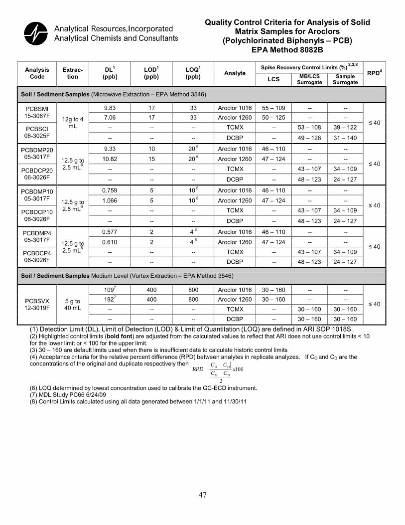
47

Analytical Resources,Incorporated Analytical Chemists and Consultants

Quality Control Criteria for Analysis of Solid Matrix Samples for Aroclors

(Polychlorinated Biphenyls – PCB) EPA Method 8082B

Analysis Code

Extrac- tion

DL1

(ppb)

LOD1

(ppb)

LOQ1

(ppb)

Analyte

Spike Recovery Control Limits (%) 2,3,8

RPD4

LCS MB/LCS Surrogate

Sample Surrogate

Soil / Sediment Samples (Microwave Extraction – EPA Method 3546)

PCBSMI 15-3067F

12g to 4 mL

9.83 17 33 Aroclor 1016 55 – 109 -- --

≤ 40

7.06 17 33 Aroclor 1260 50 – 125 -- --

PCBSCI 08-3025F

-- -- -- TCMX -- 53 – 108 39 – 122

-- -- -- DCBP -- 49 – 126 31 – 140

PCBDMP20 05-3017F

12.5 g to 2.5 mL6

9.33 10 20 6 Aroclor 1016 46 – 110 -- --

≤ 40

10.82 15 20 6 Aroclor 1260 47 – 124 -- --

PCBDCP20 06-3026F

-- -- -- TCMX -- 43 – 107 34 – 109

-- -- -- DCBP -- 48 – 123 24 – 127

PCBDMP10 05-3017F

12.5 g to 2.5 mL6

0.759 5 10 6 Aroclor 1016 46 – 110 -- --

≤ 40

1.066 5 10 6 Aroclor 1260 47 – 124 -- --

PCBDCP10 06-3026F

-- -- -- TCMX -- 43 – 107 34 – 109

-- -- -- DCBP -- 48 – 123 24 – 127

PCBDMP4 05-3017F

12.5 g to 2.5 mL6

0.577 2 4 6 Aroclor 1016 46 – 110 -- --

≤ 40

0.610 2 4 6 Aroclor 1260 47 – 124 -- --

PCBDCP4 06-3026F

-- -- -- TCMX -- 43 – 107 34 – 109 -- -- -- DCBP -- 48 – 123 24 – 127

Soil / Sediment Samples Medium Level (Vortex Extraction – EPA Method 3546)

PCBSVX 12-3019F

5 g to 40 mL

1097 400 800 Aroclor 1016 30 – 160 -- --

≤ 40

1927 400 800 Aroclor 1260 30 – 160 -- --

-- -- -- TCMX -- 30 – 160 30 – 160 -- -- -- DCBP -- 30 – 160 30 – 160

(1) Detection Limit (DL), Limit of Detection (LOD) & Limit of Quantitation (LOQ) are defined in ARI SOP 1018S. (2) Highlighted control limits (bold font) are adjusted from the calculated values to reflect that ARI does not use control limits < 10 for the lower limit or < 100 for the upper limit. (3) 30 – 160 are default limits used when there is insufficient data to calculate historic control limits (4) Acceptance criteria for the relative percent difference (RPD) between analytes in replicate analyzes. If CO and CD are the concentrations of the original and duplicate respectively then

RPD CO C D x100

CO CD

2 (6) LOQ determined by lowest concentration used to calibrate the GC-ECD instrument. (7) MDL Study PC66 6/24/09 (8) Control Limits calculated using all data generated between 1/1/11 and 11/30/11

48

Appendix B. List of analytes, methods, typical sample specific detection

level (SDL), lower method calibration limit (LMCL), on-going precision

and recovery (OPR), and replicate relative percent difference (Rep. RPD)

from AXYS Analytical Services Ltd. for water, suspended sediment, and

bed sediment samples.

Analyte Method Water Sediment

SDL LMCL OPR Rep. RPD SDL LMCL OPR Rep.

RPD

Dioxins (pg/L) (pg/L) (%) (%) (pg/L) (pg/L) (%) (%) 2,3,7,8-TCDD 1613B 0.5 10.0 70-130 ≤ 20 0.05 1.0 70-130 ≤ 20 1,2,3,7,8-PECDD 1613B 1.0 50.0 70-130 ≤ 20 0.10 5.0 70-130 ≤ 20 1,2,3,4,7,8-HXCDD 1613B 1.0 50.0 70-130 ≤ 20 0.10 5.0 70-130 ≤ 20 1,2,3,6,7,8-HXCDD 1613B 1.0 50.0 76-130 ≤ 20 0.10 5.0 76-130 ≤ 20 1,2,3,7,8,9-HXCDD 1613B 1.0 50.0 70-130 ≤ 20 0.10 5.0 70-130 ≤ 20 1,2,3,4,6,7,8-HPCDD 1613B 1.0 50.0 70-130 ≤ 20 0.10 5.0 70-130 ≤ 20 OCDD 1613B 5.0 100.0 78-130 ≤ 20 0.50 10.0 78-130 ≤ 20

Furans 2,3,7,8-TCDF 1613B 0.5 10.0 75-130 ≤ 20 0.05 1.0 75-130 ≤ 20 1,2,3,7,8-PECDF 1613B 1.0 50.0 80-130 ≤ 20 0.10 5.0 80-130 ≤ 20 2,3,4,7,8-PECDF 1613B 1.0 50.0 70-130 ≤ 20 0.10 5.0 70-130 ≤ 20 1,2,3,4,7,8-HXCDF 1613B 1.0 50.0 72-130 ≤ 20 0.10 5.0 72-130 ≤ 20 1,2,3,6,7,8-HXCDF 1613B 1.0 50.0 84-130 ≤ 20 0.10 5.0 84-130 ≤ 20 1,2,3,7,8,9-HXCDF 1613B 1.0 50.0 78-130 ≤ 20 0.10 5.0 78-130 ≤ 20 2,3,4,6,7,8-HXCDF 1613B 1.0 50.0 70-130 ≤ 20 0.10 5.0 70-130 ≤ 20 1,2,3,4,6,7,8-HPCDF 1613B 1.0 50.0 82-122 ≤ 20 0.10 5.0 82-122 ≤ 20 1,2,3,4,7,8,9-HPCDF 1613B 1.0 50.0 78-130 ≤ 20 0.10 5.0 78-130 ≤ 20 OCDF 1613B 5.0 100.0 70-130 ≤ 20 0.50 10.0 70-130 ≤ 20

Analyte Method

Water Sediment

SDL LMCL OPR Replic

ate RPD

SDL LMCL OPR Replicate RPD

PCB Congeners (pg/L) (pg/L) (%) (%) (pg/L) (pg/L) (%) (%) CL1-PCB-1 1668C 1.0 20.0 60-135 ≤ 20 0.1 2.0 60-135 ≤ 20 CL1-PCB-2 1668C 1.0 20.0 60-135 ≤ 20 0.1 2.0 60-135 ≤ 20 CL1-PCB-3 1668C 1.0 20.0 60-135 ≤ 20 0.1 2.0 60-135 ≤ 20 CL2-PCB-4 1668C 2.0 20.0 60-135 ≤ 20 0.2 2.0 60-135 ≤ 20 CL2-PCB-5 1668C 2.0 20.0 60-135 ≤ 20 0.2 2.0 60-135 ≤ 20 CL2-PCB-6 1668C 2.0 20.0 60-135 ≤ 20 0.2 2.0 60-135 ≤ 20

49

CL2-PCB-7 1668C 2.0 20.0 60-135 ≤ 20 0.2 2.0 60-135 ≤ 20 CL2-PCB-8 1668C 2.0 20.0 60-135 ≤ 20 0.2 2.0 60-135 ≤ 20 CL2-PCB-9 1668C 2.0 20.0 60-135 ≤ 20 0.2 2.0 60-135 ≤ 20 CL2-PCB-10 1668C 2.0 20.0 60-135 ≤ 20 0.2 2.0 60-135 ≤ 20 CL2-PCB-11 1668C 2.0 20.0 60-135 ≤ 20 0.2 2.0 60-135 ≤ 20 CL2-PCB-12/13 1668C 2.0 20.0 60-135 ≤ 20 0.2 2.0 60-135 ≤ 20 CL2-PCB-14 1668C 2.0 20.0 60-135 ≤ 20 0.2 2.0 60-135 ≤ 20 CL2-PCB-15 1668C 2.0 20.0 60-135 ≤ 20 0.2 2.0 60-135 ≤ 20 CL3-PCB-16 1668C 1.0 20.0 60-135 ≤ 20 0.1 2.0 60-135 ≤ 20 CL3-PCB-17 1668C 1.0 20.0 60-135 ≤ 20 0.1 2.0 60-135 ≤ 20 CL3-PCB-19 1668C 1.0 20.0 60-135 ≤ 20 0.1 2.0 60-135 ≤ 20 CL3-PCB-21/33 1668C 1.0 20.0 60-135 ≤ 20 0.1 2.0 60-135 ≤ 20 CL3-PCB-22 1668C 1.0 20.0 60-135 ≤ 20 0.1 2.0 60-135 ≤ 20 CL3-PCB-23 1668C 1.0 20.0 60-135 ≤ 20 0.1 2.0 60-135 ≤ 20 CL3-PCB-24 1668C 1.0 20.0 60-135 ≤ 20 0.1 2.0 60-135 ≤ 20 CL3-PCB-25 1668C 1.0 20.0 60-135 ≤ 20 0.1 2.0 60-135 ≤ 20 CL3-PCB-26/29 1668C 1.0 20.0 60-135 ≤ 20 0.1 2.0 60-135 ≤ 20 CL3-PCB-27 1668C 1.0 20.0 60-135 ≤ 20 0.1 2.0 60-135 ≤ 20 CL3-PCB-28/20 1668C 1.0 20.0 60-135 ≤ 20 0.1 2.0 60-135 ≤ 20 CL3-PCB-30/18 1668C 1.0 20.0 60-135 ≤ 20 0.1 2.0 60-135 ≤ 20 CL3-PCB-31 1668C 1.0 20.0 60-135 ≤ 20 0.1 2.0 60-135 ≤ 20 CL3-PCB-32 1668C 1.0 20.0 60-135 ≤ 20 0.1 2.0 60-135 ≤ 20 CL3-PCB-34 1668C 1.0 20.0 60-135 ≤ 20 0.1 2.0 60-135 ≤ 20 CL3-PCB-35 1668C 1.0 20.0 60-135 ≤ 20 0.1 2.0 60-135 ≤ 20 CL3-PCB-36 1668C 1.0 20.0 60-135 ≤ 20 0.1 2.0 60-135 ≤ 20 CL3-PCB-37 1668C 1.0 20.0 60-135 ≤ 20 0.1 2.0 60-135 ≤ 20 CL3-PCB-38 1668C 1.0 20.0 60-135 ≤ 20 0.1 2.0 60-135 ≤ 20 CL3-PCB-39 1668C 1.0 20.0 60-135 ≤ 20 0.1 2.0 60-135 ≤ 20 CL4-PCB-41/40/71 1668C 1.0 20.0 60-135 ≤ 20 0.1 2.0 60-135 ≤ 20 CL4-PCB-42 1668C 1.0 20.0 60-135 ≤ 20 0.1 2.0 60-135 ≤ 20 CL4-PCB-43 1668C 1.0 20.0 60-135 ≤ 20 0.1 2.0 60-135 ≤ 20 CL4-PCB-44/47/65 1668C 1.0 20.0 60-135 ≤ 20 0.1 2.0 60-135 ≤ 20 CL4-PCB-45/51 1668C 1.0 20.0 60-135 ≤ 20 0.1 2.0 60-135 ≤ 20 CL4-PCB-46 1668C 1.0 20.0 60-135 ≤ 20 0.1 2.0 60-135 ≤ 20 CL4-PCB-48 1668C 1.0 20.0 60-135 ≤ 20 0.1 2.0 60-135 ≤ 20 CL4-PCB-50/53 1668C 1.0 20.0 60-135 ≤ 20 0.1 2.0 60-135 ≤ 20 CL4-PCB-52 1668C 1.0 20.0 60-135 ≤ 20 0.1 2.0 60-135 ≤ 20 CL4-PCB-54 1668C 1.0 20.0 60-135 ≤ 20 0.1 2.0 60-135 ≤ 20 CL4-PCB-55 1668C 1.0 20.0 60-135 ≤ 20 0.1 2.0 60-135 ≤ 20 CL4-PCB-56 1668C 1.0 20.0 60-135 ≤ 20 0.1 2.0 60-135 ≤ 20 CL4-PCB-57 1668C 1.0 20.0 60-135 ≤ 20 0.1 2.0 60-135 ≤ 20 CL4-PCB-58 1668C 1.0 20.0 60-135 ≤ 20 0.1 2.0 60-135 ≤ 20 CL4-PCB-59/62/75 1668C 1.0 20.0 60-135 ≤ 20 0.1 2.0 60-135 ≤ 20

50

CL4-PCB-60 1668C 1.0 20.0 60-135 ≤ 20 0.1 2.0 60-135 ≤ 20 CL4-PCB-61/70/74/76 1668C 1.0 20.0 60-135 ≤ 20 0.1 2.0 60-135 ≤ 20 CL4-PCB-63 1668C 1.0 20.0 60-135 ≤ 20 0.1 2.0 60-135 ≤ 20 CL4-PCB-64 1668C 1.0 20.0 60-135 ≤ 20 0.1 2.0 60-135 ≤ 20 CL4-PCB-66 1668C 1.0 20.0 60-135 ≤ 20 0.1 2.0 60-135 ≤ 20 CL4-PCB-67 1668C 1.0 20.0 60-135 ≤ 20 0.1 2.0 60-135 ≤ 20 CL4-PCB-68 1668C 1.0 20.0 60-135 ≤ 20 0.1 2.0 60-135 ≤ 20 CL4-PCB-69/49 1668C 1.0 20.0 60-135 ≤ 20 0.1 2.0 60-135 ≤ 20 CL4-PCB-72 1668C 1.0 20.0 60-135 ≤ 20 0.1 2.0 60-135 ≤ 20 CL4-PCB-73 1668C 1.0 20.0 60-135 ≤ 20 0.1 2.0 60-135 ≤ 20 CL4-PCB-77 1668C 1.0 20.0 60-135 ≤ 20 0.1 2.0 60-135 ≤ 20 CL4-PCB-78 1668C 1.0 20.0 60-135 ≤ 20 0.1 2.0 60-135 ≤ 20 CL4-PCB-79 1668C 1.0 20.0 60-135 ≤ 20 0.1 2.0 60-135 ≤ 20 CL4-PCB-80 1668C 1.0 20.0 60-135 ≤ 20 0.1 2.0 60-135 ≤ 20 CL4-PCB-81 1668C 1.0 20.0 60-135 ≤ 20 0.1 2.0 60-135 ≤ 20 CL5-PCB-82 1668C 1.0 20.0 60-135 ≤ 20 0.1 2.0 60-135 ≤ 20 CL5-PCB-83/99 1668C 1.0 20.0 60-135 ≤ 20 0.1 2.0 60-135 ≤ 20 CL5-PCB-84 1668C 1.0 20.0 60-135 ≤ 20 0.1 2.0 60-135 ≤ 20 CL5-PCB-88/91 1668C 1.0 20.0 60-135 ≤ 20 0.1 2.0 60-135 ≤ 20 CL5-PCB-89 1668C 1.0 20.0 60-135 ≤ 20 0.1 2.0 60-135 ≤ 20 CL5-PCB-92 1668C 1.0 20.0 60-135 ≤ 20 0.1 2.0 60-135 ≤ 20 CL5-PCB-94 1668C 1.0 20.0 60-135 ≤ 20 0.1 2.0 60-135 ≤ 20 CL5-PCB-95/100/93/102/98 1668C 1.0 20.0 60-135 ≤ 20 0.1 2.0 60-135 ≤ 20 CL5-PCB-96 1668C 1.0 20.0 60-135 ≤ 20 0.1 2.0 60-135 ≤ 20 CL5-PCB-103 1668C 1.0 20.0 60-135 ≤ 20 0.1 2.0 60-135 ≤ 20 CL5-PCB-104 1668C 1.0 20.0 60-135 ≤ 20 0.1 2.0 60-135 ≤ 20 CL5-PCB-105 1668C 1.0 20.0 60-135 ≤ 20 0.1 2.0 60-135 ≤ 20 CL5-PCB-106 1668C 1.0 20.0 60-135 ≤ 20 0.1 2.0 60-135 ≤ 20 CL5-PCB-108/124 1668C 1.0 20.0 60-135 ≤ 20 0.1 2.0 60-135 ≤ 20 CL5-PCB-109/119/86/97/125/87 1668C 1.0 20.0 60-135 ≤ 20 0.1 2.0 60-135 ≤ 20 CL5-PCB-107 1668C 1.0 20.0 60-135 ≤ 20 0.1 2.0 60-135 ≤ 20 CL5-PCB-110/115 1668C 1.0 20.0 60-135 ≤ 20 0.1 2.0 60-135 ≤ 20 CL5-PCB-111 1668C 1.0 20.0 60-135 ≤ 20 0.1 2.0 60-135 ≤ 20 CL5-PCB-112 1668C 1.0 20.0 60-135 ≤ 20 0.1 2.0 60-135 ≤ 20 CL5-PCB-113/90/101 1668C 1.0 20.0 60-135 ≤ 20 0.1 2.0 60-135 ≤ 20 CL5-PCB-114 1668C 1.0 20.0 60-135 ≤ 20 0.1 2.0 60-135 ≤ 20 CL5-PCB-117/116/85 1668C 1.0 20.0 60-135 ≤ 20 0.1 2.0 60-135 ≤ 20 CL5-PCB-118 1668C 1.0 20.0 60-135 ≤ 20 0.1 2.0 60-135 ≤ 20 CL5-PCB-120 1668C 1.0 20.0 60-135 ≤ 20 0.1 2.0 60-135 ≤ 20 CL5-PCB-121 1668C 1.0 20.0 60-135 ≤ 20 0.1 2.0 60-135 ≤ 20 CL5-PCB-122 1668C 1.0 20.0 60-135 ≤ 20 0.1 2.0 60-135 ≤ 20

51

CL5-PCB-123 1668C 1.0 20.0 60-135 ≤ 20 0.1 2.0 60-135 ≤ 20 CL5-PCB-126 1668C 1.0 20.0 60-135 ≤ 20 0.1 2.0 60-135 ≤ 20 CL5-PCB-127 1668C 1.0 20.0 60-135 ≤ 20 0.1 2.0 60-135 ≤ 20 CL6-PCB-128/166 1668C 1.0 20.0 60-135 ≤ 20 0.1 2.0 60-135 ≤ 20 CL6-PCB-130 1668C 1.0 20.0 60-135 ≤ 20 0.1 2.0 60-135 ≤ 20 CL6-PCB-131 1668C 1.0 20.0 60-135 ≤ 20 0.1 2.0 60-135 ≤ 20 CL6-PCB-132 1668C 1.0 20.0 60-135 ≤ 20 0.1 2.0 60-135 ≤ 20 CL6-PCB-133 1668C 1.0 20.0 60-135 ≤ 20 0.1 2.0 60-135 ≤ 20 CL6-PCB-134/143 1668C 1.0 20.0 60-135 ≤ 20 0.1 2.0 60-135 ≤ 20 CL6-PCB-136 1668C 1.0 20.0 60-135 ≤ 20 0.1 2.0 60-135 ≤ 20 CL6-PCB-137 1668C 1.0 20.0 60-135 ≤ 20 0.1 2.0 60-135 ≤ 20 CL6-PCB-138/163/129/160 1668C 1.0 20.0 60-135 ≤ 20 0.1 2.0 60-135 ≤ 20 CL6-PCB-139/140 1668C 1.0 20.0 60-135 ≤ 20 0.1 2.0 60-135 ≤ 20 CL6-PCB-141 1668C 1.0 20.0 60-135 ≤ 20 0.1 2.0 60-135 ≤ 20 CL6-PCB-142 1668C 1.0 20.0 60-135 ≤ 20 0.1 2.0 60-135 ≤ 20 CL6-PCB-144 1668C 1.0 20.0 60-135 ≤ 20 0.1 2.0 60-135 ≤ 20 CL6-PCB-145 1668C 1.0 20.0 60-135 ≤ 20 0.1 2.0 60-135 ≤ 20 CL6-PCB-146 1668C 1.0 20.0 60-135 ≤ 20 0.1 2.0 60-135 ≤ 20 CL6-PCB-147/149 1668C 1.0 20.0 60-135 ≤ 20 0.1 2.0 60-135 ≤ 20 CL6-PCB-148 1668C 1.0 20.0 60-135 ≤ 20 0.1 2.0 60-135 ≤ 20 CL6-PCB-150 1668C 1.0 20.0 60-135 ≤ 20 0.1 2.0 60-135 ≤ 20 CL6-PCB-151/135/154 1668C 1.0 20.0 60-135 ≤ 20 0.1 2.0 60-135 ≤ 20 CL6-PCB-152 1668C 1.0 20.0 60-135 ≤ 20 0.1 2.0 60-135 ≤ 20 CL6-PCB-153/168 1668C 1.0 20.0 60-135 ≤ 20 0.1 2.0 60-135 ≤ 20 CL6-PCB-155 1668C 1.0 20.0 60-135 ≤ 20 0.1 2.0 60-135 ≤ 20 CL6-PCB-156/157 1668C 1.0 40.0 60-135 ≤ 20 0.1 4.0 60-135 ≤ 20 CL6-PCB-158 1668C 1.0 20.0 60-135 ≤ 20 0.1 2.0 60-135 ≤ 20 CL6-PCB-159 1668C 1.0 20.0 60-135 ≤ 20 0.1 2.0 60-135 ≤ 20 CL6-PCB-161 1668C 1.0 20.0 60-135 ≤ 20 0.1 2.0 60-135 ≤ 20 CL6-PCB-162 1668C 1.0 20.0 60-135 ≤ 20 0.1 2.0 60-135 ≤ 20 CL6-PCB-164 1668C 1.0 20.0 60-135 ≤ 20 0.1 2.0 60-135 ≤ 20 CL6-PCB-165 1668C 1.0 20.0 60-135 ≤ 20 0.1 2.0 60-135 ≤ 20 CL6-PCB-167 1668C 1.0 20.0 60-135 ≤ 20 0.1 2.0 60-135 ≤ 20 CL6-PCB-169 1668C 1.0 20.0 60-135 ≤ 20 0.1 2.0 60-135 ≤ 20 CL7-PCB-170 1668C 1.0 20.0 60-135 ≤ 20 0.1 2.0 60-135 ≤ 20 CL7-PCB-171/173 1668C 1.0 20.0 60-135 ≤ 20 0.1 2.0 60-135 ≤ 20 CL7-PCB-172 1668C 1.0 20.0 60-135 ≤ 20 0.1 2.0 60-135 ≤ 20 CL7-PCB-174 1668C 1.0 20.0 60-135 ≤ 20 0.1 2.0 60-135 ≤ 20 CL7-PCB-175 1668C 1.0 20.0 60-135 ≤ 20 0.1 2.0 60-135 ≤ 20 CL7-PCB-176 1668C 1.0 20.0 60-135 ≤ 20 0.1 2.0 60-135 ≤ 20 CL7-PCB-177 1668C 1.0 20.0 60-135 ≤ 20 0.1 2.0 60-135 ≤ 20 CL7-PCB-178 1668C 1.0 20.0 60-135 ≤ 20 0.1 2.0 60-135 ≤ 20

52

CL7-PCB-179 1668C 1.0 20.0 60-135 ≤ 20 0.1 2.0 60-135 ≤ 20 CL7-PCB-180/193 1668C 1.0 20.0 60-135 ≤ 20 0.1 2.0 60-135 ≤ 20 CL7-PCB-181 1668C 1.0 20.0 60-135 ≤ 20 0.1 2.0 60-135 ≤ 20 CL7-PCB-182 1668C 1.0 20.0 60-135 ≤ 20 0.1 2.0 60-135 ≤ 20 CL7-PCB-183/185 1668C 1.0 20.0 60-135 ≤ 20 0.1 2.0 60-135 ≤ 20 CL7-PCB-184 1668C 1.0 20.0 60-135 ≤ 20 0.1 2.0 60-135 ≤ 20 CL7-PCB-186 1668C 1.0 20.0 60-135 ≤ 20 0.1 2.0 60-135 ≤ 20 CL7-PCB-187 1668C 1.0 20.0 60-135 ≤ 20 0.1 2.0 60-135 ≤ 20 CL7-PCB-188 1668C 1.0 20.0 60-135 ≤ 20 0.1 2.0 60-135 ≤ 20 CL7-PCB-189 1668C 1.0 20.0 60-135 ≤ 20 0.1 2.0 60-135 ≤ 20 CL7-PCB-190 1668C 1.0 20.0 60-135 ≤ 20 0.1 2.0 60-135 ≤ 20 CL7-PCB-191 1668C 1.0 20.0 60-135 ≤ 20 0.1 2.0 60-135 ≤ 20 CL7-PCB-192 1668C 1.0 20.0 60-135 ≤ 20 0.1 2.0 60-135 ≤ 20 CL8-PCB-194 1668C 1.0 20.0 60-135 ≤ 20 0.1 2.0 60-135 ≤ 20 CL8-PCB-195 1668C 1.0 20.0 60-135 ≤ 20 0.1 2.0 60-135 ≤ 20 CL8-PCB-196 1668C 1.0 20.0 60-135 ≤ 20 0.1 2.0 60-135 ≤ 20 CL8-PCB-197/200 1668C 1.0 20.0 60-135 ≤ 20 0.1 2.0 60-135 ≤ 20 CL8-PCB-198/199 1668C 1.0 20.0 60-135 ≤ 20 0.1 2.0 60-135 ≤ 20 CL8-PCB-201 1668C 1.0 20.0 60-135 ≤ 20 0.1 2.0 60-135 ≤ 20 CL8-PCB-202 1668C 1.0 20.0 60-135 ≤ 20 0.1 2.0 60-135 ≤ 20 CL8-PCB-203 1668C 1.0 20.0 60-135 ≤ 20 0.1 2.0 60-135 ≤ 20 CL8-PCB-204 1668C 1.0 20.0 60-135 ≤ 20 0.1 2.0 60-135 ≤ 20 CL8-PCB-205 1668C 1.0 20.0 60-135 ≤ 20 0.1 2.0 60-135 ≤ 20 CL9-PCB-206 1668C 1.0 20.0 60-135 ≤ 20 0.1 2.0 60-135 ≤ 20 CL9-PCB-207 1668C 1.0 20.0 60-135 ≤ 20 0.1 2.0 60-135 ≤ 20 CL9-PCB-208 1668C 1.0 20.0 60-135 ≤ 20 0.1 2.0 60-135 ≤ 20 CL10-PCB-209 1668C 1.0 20.0 60-135 ≤ 20 0.1 2.0 60-135 ≤ 20