guidance for assessing bioaccumulative chemicals … for assessing bioaccumulative chemicals of...
TRANSCRIPT

Guidance for Assessing Bioaccumulative Chemicals of Concern in Sediment January 31, 2007
April 3, 2007 – Updated
October 2017 – Updated format, contact information, and website links
Environmental Cleanup Program 700 NE Multnomah St.
Suite 600 Portland, OR 97232
Phone: 503-229-6258
800-452-4011 Fax: 503-229-5850
Contact: Tiffany Johnson
www.oregon.gov/DEQ
DEQ is a leader in
restoring, maintaining and
enhancing the quality of
Oregon’s air, land and
water.
Guidance for Assessing Bioaccumulative Chemicals of Concern in Sediment
State of Oregon Department of Environmental Quality ii
Documents can be provided upon request in an alternate format for individuals with disabilities or in a
language other than English for people with limited English skills. To request a document in another
format or language, call DEQ in Portland at 503-229-5696, or toll-free in Oregon at 1-800-452-4011, ext.
5696; or email [email protected].
Guidance for Assessing Bioaccumulative Chemicals of Concern in Sediment
State of Oregon Department of Environmental Quality iii
I. ACKNOWLEDGEMENTS
This document was developed with the help of the Sediment Technical Advisory Panel and DEQ staff and
contractor:
Pamela Bridgen, Environment International, Ltd.
Rebekah Brooks, Landau Associates, Inc.
Jeremy Buck, U.S. Fish & Wildlife Service
Rick Cardwell, Parametrix
Taku Fuji, Kennedy/Jenks Consultants
Jane Harris, Oregon Center for Environmental Health
Lyndal L. Johnson, National Oceanic & Atmospheric Administration
James McKenna, Port of Portland
Peter Rude, formerly Landau Associates, Inc.
Mark Siipola, U.S. Army Corps of Engineers
Robert Wyatt, NW Natural
Jim Anderson, DEQ, Northwest Region Environmental Cleanup Program
Michael R. Anderson, DEQ, Northwest Region Environmental Cleanup Program
Martin Fitzpatrick, DEQ, Water Quality Program
Bruce Gilles, DEQ, Northwest Region Environmental Cleanup Program
Ray Hoy, DEQ, Northwest Region Environmental Cleanup Program
Keith Johnson, DEQ, Northwest Region Environmental Cleanup Program
Ann Levine, DEQ, Land Quality Division Environmental Cleanup Program
Angie Obery, DEQ, Western Region Environmental Cleanup Program
Jennifer Peterson, DEQ, Northwest Region Environmental Cleanup Program
Mike Poulsen, DEQ, Northwest Region Environmental Cleanup Program
Jennifer Sutter, DEQ, Northwest Region Environmental Cleanup Program
Neil Morton, GeoEngineers, Inc.
Additional review was provided by DEQ cleanup program managers and staff. Members of the public
were invited to review and comment on the September 29, 2006, draft of this document. Their
suggestions were considered and incorporated where appropriate into this guidance document.
II. APPROVAL
This guidance document has been approved for use by the Department of Environmental Quality Land
Quality Division.
____[Alan Kiphut]_____________________ _1/31/2007______________
Alan Kiphut, Division Administrator Date

Guidance for Assessing Bioaccumulative Chemicals of Concern in Sediment
State of Oregon Department of Environmental Quality iv
Table of Contents I. Acknowledgements .......................................................................................................................... iii
II. Approval ............................................................................................................................................ iii
1. Introduction ....................................................................................................................................... 1
2. Summary of the Process................................................................................................................... 3
2.1 Investigation of the Site ............................................................................................................... 3 2.2 Evaluation of Bioaccumulation .................................................................................................... 4 2.3 Outline of the Process................................................................................................................. 7
3. Contaminants of Interest .................................................................................................................. 8
4. Sediment Screening Levels .............................................................................................................. 9
4.1 Generic Sediment Screening Levels ........................................................................................... 9 4.2 Site-Specific Sediment Screening Levels .................................................................................. 11
5. Acceptable Fish Tissue Levels ....................................................................................................... 12
5.1 Acceptable Tissue Levels ......................................................................................................... 12 5.2 Determining Tissue Levels ........................................................................................................ 13 5.2.1 Using Fish/Shellfish -Tissue Data .................................................................................. 13 5.2.2 Bioaccumulation Bioassays ........................................................................................... 15
6. Response Actions ........................................................................................................................... 15
6.1 If A Bioaccumulator Is Detected ................................................................................................ 15 6.2 If No Bioaccumulator Is Detected .............................................................................................. 17 6.3 Compliance Monitoring ............................................................................................................. 18
Appendix A. ......................................................................................................................................... A-0
Tables for Bioaccumulation Screening ............................................................................................. A-0
Appendix B. ......................................................................................................................................... B-1
Regional Default Background Concentrations ................................................................................. B-1
for Soil/Sediment ................................................................................................................................. B-1
Regional Default Background Concentrations for Soil/Sediment ................................................... B-1
Appendix C. ......................................................................................................................................... C-1
Calculating Acceptable Tissue Levels ............................................................................................... C-1
& C-1
Critical Tissue Levels .......................................................................................................................... C-1
C.1 Acceptable Tissue Levels for Humans .................................................................................... C-1 C.2 Acceptable Tissue Levels for Wildlife ...................................................................................... C-2 C.3 Critical Tissue Levels for Fish ................................................................................................. C-5 C.3.1 WQC x BCF Method .................................................................................................................... C-5 C.3.2 SSD Method Data Compilation .................................................................................................... C-8 C.3.3 SSD Method Calculations ......................................................................................................... C-10 C.3.4 CTL Comparison ....................................................................................................................... C-13 C.4 References for Appendix C ................................................................................................... C-14

Guidance for Assessing Bioaccumulative Chemicals of Concern in Sediment
State of Oregon Department of Environmental Quality v
Appendix D. ......................................................................................................................................... D-0
D. Deriving Bioaccumulation Screening Level Values .................................................................... D-1
D.1 Wildlife Receptors ................................................................................................................... D-1 D.1.1 Organic Chemicals ...................................................................................................... D-1 D.1.2 Inorganic Chemicals .................................................................................................... D-3 D.2 Human Receptors ................................................................................................................... D-4 D.2.1 Organic Chemicals ...................................................................................................... D-4 D.2.2 Inorganic Chemicals .................................................................................................... D-4 D.2.3 SLVs for Populations Other Than the General Population ........................................... D-4 D.3 Fish and Other Aquatic Receptors .......................................................................................... D-5 D.3.1 Organic Chemicals ...................................................................................................... D-5 D.3.2 Inorganic Chemicals .................................................................................................... D-5
Appendix E. ......................................................................................................................................... E-0
Bioaccumulation Test Methods.......................................................................................................... E-0
E.1 Using Standard Test Organisms ............................................................................................. E-1 E.1.1 Freshwater Tests ........................................................................................................ E-1 E.1.2 Marine / Estuarine Tests ............................................................................................. E-2 E.2 Using Caged Test Organisms ................................................................................................. E-2
Appendix F.F-1
Data and Graph for Example 2 ............................................................................................................F-1
Appendix G. ......................................................................................................................................... G-1
References G-1
List of Figures
Figure 1 An Example of a Food-Web ....................................................................................................... 2 Figure 2 Simplified Food Web Showing Pathways Discussed in this Document ....................................... 5 Figure 3 Assessing Chemicals for Bioaccumulation ................................................................................. 6 Figure F-1 Using a Graph to Determine Ambient/Baseline Concentrations ............................................F-1
List of Tables Table A-1a: Sediment Bioaccumulation Screening Level Values (SLVs) ............................................... A-1 Table A-1b: SLVs for Designated Dioxin/Furan and PCB Congeners .................................................... A-2 Table A-2a: Exposure Parameters Used to Calculate Screening Level Values ..................................... A-4 Table A-2b: Table: Human Toxicity Values Used to Calculate Screening Level Values ......................... A-5 Table A-3a: Acceptable Tissue Levels (ATLs) for Chemicals in Fish/Shellfish Consumed by Wildlife and Humans................................................................................................................................................. A-6 Table A-3b: ATLs for Selected Dioxin/Furan Congeners in Fish/Shellfish Consumed by Wildlife and Humans................................................................................................................................................. A-7 Table A-4: CTLs for Chemicals in Fish, Shellfish, and Other Aquatic Organisms .................................. A-9 Table A-5a: Default Uptake Values for Estimating Concentrations in Fish Tissue ............................... A-10 Table A-5b: Default Uptake Values for Values for Designated Congeners .......................................... A-11 Table A-6a: Table: Toxicity Reference Values (TRVs)......................................................................... A-12 Table A-6b: Toxicity Reference Values for Designated Congeners ..................................................... A-13 Table A-7: Analytical Methods and Reporting Limits ........................................................................... A-15

Guidance for Assessing Bioaccumulative Chemicals of Concern in Sediment
State of Oregon Department of Environmental Quality vi
Table B-1: Oregon DEQ Suggested Default Background Concentrations for Inorganic Contaminants in Soil/Sediment ........................................................................................................................................ B-1 Table C-1: Sources of Data for CTL Calculations ................................................................................ C-17 Table C-2: Bioconcentration Factors WQC x BCF Method……………………………………...C-18 Table C-3: Water Quality Criteria - Federal and International…………...………………………C-19 Table C-4: Water Quality Criteria for Fluoranthene, Hexachlorobenzene and Pyrene by State ....................... C-20 TABLE C-5: NOER/LOER Database Summary ................................................................................... C-21 TABLE C-6: Critical Tissue Levels Check ............................................................................................ C-22
List of Acronyms
90UCL 90% Upper confidence level of the mean
ATLh Acceptable tissue levels for humans
ATLhC Acceptable tissue levels of carcinogens for humans
ATLhN Acceptable tissue levels of noncarcinogens for humans
ATL Acceptable tissue level
ATLw Acceptable tissue levels for wildlife
ATLw-egg Acceptable tissue levels for egg development
AWQC Ambient water quality criteria
BCF Bioconcentration factor
BCOI Bioaccumulative contaminant of interest
BMF Biomagnification factor
BMFegg Biomagnification factor for egg development
BSAF Biota-sediment accumulation factor (for organic chemicals)
CASRN Chemical Abstracts Service Registry Number
CBAC Cumulative bioaccumulation index for an individual chemical;
COI Contaminant of interest
COPC Contaminant of potential concern
CRITFC Columbia River Inter-Tribal Fish Commission
CSM Conceptual site model
CTL Critical tissue level (for fish)
DEQ Department of Environmental Quality
DQO Data quality objectives
ECtissue Equilibrium contaminant tissue concentration in fish
EE/CA Engineering evaluation/cost assessment
EPC Exposure point concentration
foc Fraction of organic carbon in the sediment
fL Fraction of lipid content in the organism
FS Feasibility study
IQR Interquartile Range
Kd Distribution coefficient for inorganics

Guidance for Assessing Bioaccumulative Chemicals of Concern in Sediment
State of Oregon Department of Environmental Quality vii
MDL Method detection limit
mg/kg ww The mg/kg concentration is based on the wet weight of the sample
N Total number of contaminants in sediment at the site
ND Non detect
NFA No further action
OAR Oregon Administrative Rule
PAHs Polynuclear Aromatic Hydrocarbons
RBAC Bioaccumulation index for each individual chemical in the sediment
RI Remedial Investigation
SLV Screening level value
SLVBH Sediment bioaccumulation screening level for humans
SLVBW Sediment bioaccumulation screening level for wildlife
SSD Species sensitivity distribution
T&E Threatened or endangered
TRV Toxicity Reference Value
UCL Upper confidence limit of the arithmetic mean
90UCL 90% upper confidence limit of the arithmetic mean

Guidance for Assessing Bioaccumulative Chemicals of Concern in Sediment
State of Oregon Department of Environmental Quality 1
1. INTRODUCTION
This document describes a process used by the Oregon Department of Environmental Quality (DEQ) to
evaluate chemicals found in sediment for their potential contribution to risk as a result of
bioaccumulation. It is presented here as an example of a method that others may use for that purpose,
if appropriate. Its use, however, is not required.
The revised environmental cleanup law and associated administrative rules adopted by the
Environmental Quality Commission in 1997 provide that any removal or remedial action
performed under the law and rules shall attain a degree of cleanup of the hazardous substance
and control further release of the hazardous substance that assures protection of present and
future public health, safety and welfare and of the environment.
This guidance describes several ways to determine if hazardous substances released to sediment
have the potential to bioaccumulate to the point where the contaminants adversely affect either
the health of the fish or other aquatic organisms, or the health of animals or humans that
consume them.
This guidance supplements existing risk assessment guidance, and only addresses the evaluation
of bioaccumulative chemicals in sediment. Guidance documents for assessing risk to human
health (DEQ, 2000) or ecological receptors (DEQ, 2001b) provide the framework for the
complete risk assessment process.
Bioaccumulation is a general term applied when there is a net accumulation of a chemical by an
organism as a result of uptake from all routes of exposure. As used in this document, the term
bioaccumulation includes bioconcentration, which is the net accumulation of a dissolved
chemical directly from water by an aquatic organism, and biomagnification, which refers to the
process by which chemicals tend to accumulate to higher concentrations at higher levels in the
food web due to dietary accumulation.1
Bioaccumulation of contaminants from sediments to benthic organisms and their subsequent
transfer through the food web provides an exposure pathway to higher-level organisms (Figure
1). Because sediments can contain significantly higher concentrations of some chemicals than
the overlying water, it is important to evaluate the potential for such chemicals to accumulate in
aquatic organisms. This information is needed to help predict potentially adverse effects on fish,
shellfish, and other aquatic prey animals, or on wildlife or humans that consume them.
1 Chemicals that biomagnify generally create more risk than those that only bioconcentrate. Many metals
bioconcentrate to varying degrees but do not biomagnify like PCBs, DDT, and dioxin.

Guidance for Assessing Bioaccumulative Chemicals of Concern in Sediment
State of Oregon Department of Environmental Quality 2
Figure 1. An Example of a Food-Web

Guidance for Assessing Bioaccumulative Chemicals of Concern in Sediment
State of Oregon Department of Environmental Quality 3
Since Oregon's Environmental Cleanup Rules require responsible parties to evaluate
contaminants capable of bioaccumulation,2 this guidance is designed to help you:
Recognize options for evaluating the bioaccumulation potential of chemicals;
Identify chemicals in sediment that could present a bioaccumulation risk; and
Estimate the likelihood that these chemicals pose a threat to humans or wildlife as a result of
eating fish, shellfish, and other aquatic organisms from a particular location. Chemicals
identified as bioaccumulative compounds in this guidance were developed through a consensus-
based process with the Regional Sediment Evaluation Team (RSET), which is developing
screening levels to guide disposal options for dredged sediment, and review of more recent fish
tissue testing results from the lower Willamette basin3. The toxicity of those chemicals and
chemicals that do not bioaccumulate must also be addressed in the risk assessment. Both must
be evaluated at sites with contaminated sediment since neither is a predictor of the presence or
consequences of the other. Further, the bioaccumulation related risks and toxicity of
contaminants in sediment need to be considered within the overall risk assessment for a facility
that addresses all impacted media and routes of exposure. For additional assistance consult
DEQ's Guidance for Ecological Risk Assessment (DEQ, 2001b) and Guidance for Conduct of
Deterministic Human Health Risk Assessments (DEQ, 2000). This document does not address
the evaluation of the interface between contaminated groundwater and sediment, or the
evaluation of potential toxic effects from the bioconcentration of Polynuclear Aromatic
Hydrocarbons (PAHs) and metals in benthic organisms. If these pathways are a concern, please
contact your DEQ project manager.
2. SUMMARY OF THE PROCESS
2.1 INVESTIGATION OF THE SITE
As with any remedial investigation (RI), it is very important that you determine the full
magnitude and extent of the contamination and identify all contaminants of interest at the site.
The preliminary conceptual site model (CSM) that illustrates the potential current and reasonably
likely future exposures to human and ecological receptors will support the development of data
quality objectives4 (DQOs) for the RI. DQOs should be consistent with the DEQ Cleanup
Program Quality Assurance Policy (DEQ, 2001a) to ensure the data is of sufficient quality to
2 Oregon Administrative Rules (OAR) 340-122-084(3)(d) requires “…information regarding the toxicological effects,
ecological effects, bioconcentration potential, bioaccumulation potential, biomagnification potential, and persistence of the identified contaminants of ecological concern, …”
3 The list of bioaccumative compounds specifically identified in this guidance may be expanded by DEQ on a project
specific basis where high concentrations of a hazardous substance possessing chemical properties consistent with the criteria used in the RSET process has been detected in sediment and has been detected in fish tissue studies conducted elsewhere in the watershed.
4 Additional information on the DQO process can be viewed at http://www.hanford.gov/dqo/index.html

Guidance for Assessing Bioaccumulative Chemicals of Concern in Sediment
State of Oregon Department of Environmental Quality 4
apply this guidance and complete the risk assessment. The DQO development will need to
address analytical requirements such as method detection limits (see Table A-7), and background
concentrations of naturally occurring elements (see Appendix B). In this guidance document we
assume that you have already completed the CSM and DQO development tasks satisfactorily.
Before you can evaluate the potential for bioaccumulation you need to determine if any
individuals of a threatened or endangered (T&E) aquatic or terrestrial fish-eating species or their
critical habitat are present within the locality of the facility using the methodology provided in
DEQ's Guidance for Ecological Risk Assessment (DEQ, 2001b). This is necessary in order to
determine what set of screening levels apply to your site. If there is no current or reasonably
likely future use of the locality of the facility by a T&E species, use numbers from the
“Population” column in the "Birds" or "Mammals" sections of tables referred to later in this
document. If you cannot rule out the presence of a T&E species with reasonable certainty, use
the numbers from the “Individual” columns in the tables.
In urban settings, determining the LOF may be complicated or inconclusive due to widespread
presence of elevated levels of chemicals in sediment upstream of the facility that exceed the
screening criteria in this guidance. Under these circumstances, you should consult with the DEQ
project manager and toxicologist on how to complete the bioaccumulation screening and/or
develop the feasible removal or remedial action options to address site-specific contamination
that exceeds both the screening and ambient levels. Also see Example 3, Section 6 below.
2.2 EVALUATION OF BIOACCUMULATION
Since food webs can be quite complex, for the purposes of this guidance document we will focus
only on the relationships illustrated in Figure 2. We would like to determine if the
concentrations of contaminants in sediment are high enough to bioaccumulate in fish and other
aquatic organisms to the point where the contaminants affect either the health of humans or
animals that consume the fish or other aquatic organisms, or the health of the aquatic organisms
themselves. The methods discussed in this document evaluate potential bioaccumulation by:
Comparing the measured concentration of contaminants in sediment to sediment screening
level values (SLVs) for humans and relevant classes of wildlife;
Comparing the estimated or measured concentration of contaminants in fish tissue to
acceptable tissue levels (ATLs) for humans and relevant classes of wildlife and/or to
critical tissue levels (CTLs) in fish;
Measuring bioaccumulation with laboratory or in situ tests; or
Modeling bioaccumulation with site-specific fish or benthic invertebrate tissue data and a
food web model.
The steps described in this guidance document are outlined in Section 2.3 and illustrated in
Figure 3.

Guidance for Assessing Bioaccumulative Chemicals of Concern in Sediment
State of Oregon Department of Environmental Quality 5
Note: For convenience, the process discussed in Section 2.3 is presented in a traditional “tiered”
format, starting with the easiest, least costly, and most generic methods and proceeding up to more
detailed, more costly, and more site-specific methods. You are not, however, required to perform all of
the steps or follow the suggested order.
Fish and benthic
invertebrates
Birds HumansMammals
Contaminants in
Sediment
Figure 2. Simplified Food Web Showing Pathways Discussed in this Document

Guidance for Assessing Bioaccumulative Chemicals of Concern in Sediment
State of Oregon Department of Environmental Quality 6
Figure 3. Assessing Chemicals for Bioaccumulation
NFA for bioaccumulation
Change generic exposure parameters to calculate
site-specific SLVs
Perform one of the following
No
No
Yes
Yes
Use existing data to identify COIs that may bioaccumulate (BCOI)
Complete FS for Remedial Action or EE/CA for Removal
Action
Identify contaminants of interest (COI)
Yes
Perform lab or in situ
bioaccumulation tests
No
No
Yes
Yes
No
or
Option : Calculate site- specific SLVs?
Option : Carry out additional site investigation?
Evaluate data against generic or site-specific ATLh, ATLw, and CTLs
Collect new aquatic organism
data
1
2
3b
5
4a
4b
4bii 4bi
3a
Investigate site and develop preliminary conceptual site model (CSM)
Do results indicate that bioaccumulation is
a concern?
Are BCOI concentrations less than
generic SLVs?
3
Are BCOI concentrations less than
site-specific SLVs?
4
Conduct post-remediation monitoring
6
Note: You are not
required to perform
all of these steps, or
follow the suggested
order.

Guidance for Assessing Bioaccumulative Chemicals of Concern in Sediment
State of Oregon Department of Environmental Quality 7
2.3 OUTLINE OF THE PROCESS
1. Identify the contaminants of interest (COIs) in sediment at the site.
2. Use existing data to determine which COIs, if any, are bioaccumulating contaminants of
interest (BCOIs). Table 1 shows the BCOIs that DEQ is considering. This list was
compiled using the approach developed by EPA and incorporated as List 1 in the Interim
Final Northwest Regional Sediment Evaluation Framework (USEPA/USACE 2006)
3. Compare the concentration of each BCOI in sediment at each location to its generic
bioaccumulation screening level value. If the concentration is lower, no further action is
required with respect to bioaccumulation for that COI. If the BCOI concentration is
greater than its generic SLV, consider an area-wide statistical evaluation of the exposure
point concentration taking into account the appropriate range of relevant species. This is
consistent with DEQ's general screening approach, using the maximum concentration, or
the 90 percent upper confidence limit of the arithmetic mean, whichever is lower.
However, for benthic organisms that are stationary or range over small distances, a
comparison with the maximum concentration is appropriate. If the BCOI concentration
is still greater than its generic SLV, do one of the following:
a. Evaluate the feasibility of cleaning up areas exceeding SLV levels to the generic SLV
or to non-detect5 (ND), whichever is higher, or, for a naturally occurring chemical, to
its background concentration.6 Do this by either
i. A feasibility study and a remedial action, or
ii. An engineering evaluation/cost analysis and a removal; or
b. Use information from the site along with the equations for the generic SLVs to
calculate a site-specific SLV and then continue with Step 4.
4. Compare the concentration of each BCOI in sediment at each location to its site-specific
bioaccumulation screening level value. If the concentration is lower, no further action is
required with respect to bioaccumulation for that COI. If the BCOI concentration is
greater than its site-specific SLV, consider an area-wide statistical evaluation of the
exposure point concentration taking into account the appropriate range of relevant
species. This is consistent with DEQ's general screening approach, using the maximum
concentration, or the 90 percent upper confidence limit of the arithmetic mean, whichever
5 Analytical method reporting limits (MRLs) must be considered when the data quality objectives (DQOs) are
developed for a sediment investigation. In many cases the reporting or quantitation limits of approved methods, such as those found in EPA’s SW-846, are below the bioaccumulation SLV. For some compounds the SLV is below the lowest attainable reporting limits with cleanup procedures for sample extracts to eliminate matrix interferences. Only under these circumstances, would DEQ consider using the MRL as a cleanup goal.
6 OAR 340-122-0115(8) defines background as “the concentration of hazardous substance, if any, existing in the
environment in the location of the facility before the occurrence of any past or present release or releases.”

Guidance for Assessing Bioaccumulative Chemicals of Concern in Sediment
State of Oregon Department of Environmental Quality 8
is lower. However, for benthic organisms that are stationary or range over small
distances, a comparison with the maximum concentration is appropriate. If the BCOI
concentration is still greater than its site-specific SLV, do one of the following:
a. Evaluate the feasibility of cleaning up areas exceeding SLV levels to the site-specific
SLV or to ND, whichever is higher, or, for a naturally occurring chemical, to its
background concentration. Do this by either
i. A feasibility study and a remedial action, or
ii. An engineering evaluation/cost analysis and a removal; or
b. Collect data on the concentration of BCOIs in fish or benthic invertebrate tissue
using one of the following methods, and then continue with Step 5.
i. Collect existing tissue data from an area that is applicable to your site (e.g., has
appropriate fish home range and analytes) or data from fish caught or benthic
invertebrates collected at your site for this purpose; or
ii. Perform laboratory or in situ bioaccumulation tests on sediment from the site.
5. Compare the estimated or measured concentration of each BCOI in fish or benthic
invertebrate tissue to appropriate acceptable tissue levels (ATLw and ATLh) or critical
tissue levels (CTL). If the concentration is lower, no further action is required with
respect to bioaccumulation for that COI and you should continue with a regular toxicity
evaluation. If the BCOI concentration is greater than the ATL or CTL, the COI must be
considered a chemical of potential concern (COPC) with respect to bioaccumulation and
must be cleaned up to a bioaccumulation-based level or to ND, whichever is higher; or,
for a naturally occurring compound, to its background concentration. Do this by either
a A feasibility study and a remedial action, or
b An engineering evaluation/cost analysis and a removal action.
6. Monitor the site to confirm that the goals of your remedy have been met.
The steps summarized above are described in more detail in Sections 3 - 6.
3. CONTAMINANTS OF INTEREST
Use historical information about your site as well as data collected during the site investigation
to compile a list of COIs. From the list of COIs, develop a list of BCOIs for the sediment at the
site by considering factors like:
The release of potentially bioaccumulative chemicals like arsenic, cadmium, chlordane,
DDT, dieldrin, dioxins and furans, fluoranthene, hexachlorobenzene, lead, mercury,
pentachlorophenol, PCBs, pyrene, selenium, and tributyltin;

Guidance for Assessing Bioaccumulative Chemicals of Concern in Sediment
State of Oregon Department of Environmental Quality 9
All potential sources of contamination at the site including stormwater runoff;
Pervasive legacy chemicals like PCBs and pesticides; and
Tissue data from fish and other aquatic species in the vicinity of your site.
Screen the chemicals on your BCOI list by following the procedures in Sections 4 - 6.
4. SEDIMENT SCREENING LEVELS
4.1 GENERIC SEDIMENT SCREENING LEVELS
Note: If adequate fish/shellfish-tissue data are already available, you may be able to skip the initial
screening steps and go directly to the tests discussed in Section 5.
When screening for potential bioaccumulative chemicals, you must consider risk from exposure
not only to individual contaminants, but also to multiple contaminants present together in
sediment.7 For fish and mobile fish-eating species, use the 90% upper confidence limit of the
arithmetic mean (90UCL8) sediment concentration or the maximum sediment concentration,
whichever is less, as the appropriate exposure point concentration (EPC).
To determine exposures to individual chemicals, compare the EPC of each bioaccumulative COI
in the sediment to its generic SLV or to natural background concentration listed in Table A-1 in
Appendix A. This relationship, the bioaccumulation index (RBAC), is defined by the following
equation:
SLV
EPCRBAC [1]
where:
RBAC = bioaccumulation index for an individual COI (unitless);
EPC = exposure point concentration of a given COI in sediment (mg/kg); and
SLV = screening level value for the COI (mg/kg) and receptor class from Table A-1.
7 This is "cumulative risk" as described in OAR 340-122-084(1)(i).
8 You can calculate 90UCL with spreadsheets available on the Internet from either the DEQ
(http://www.oregon.gov/deq/tanks/Pages/Upper-Limit.aspx or http://www.oregon.gov/deq/Hazards-and-Cleanup/env-cleanup/Pages/Risk-Based-Decision-Making.aspx) or the EPA (http://www.epa.gov/nerlesd1/tsc/software.htm).

Guidance for Assessing Bioaccumulative Chemicals of Concern in Sediment
State of Oregon Department of Environmental Quality 10
If the RBAC is greater than 1 for any individual COI, that chemical is a contaminant of potential
concern (COPC) on the basis of the generic SLVs and could be a bioaccumulation threat to
humans or wildlife that consume fish, shellfish, and other aquatic organisms.
Next, determine if there is a potential for a group of two or more contaminants to generate
cumulative bioaccumulation risk.9 To do this, add up the RBAC values for a particular receptor
class.10 If the sum is less than 1 there is no unacceptable cumulative risk as a result of
bioaccumulation.
If the sum of all of the RBAC values is greater than 1, examine the value of RBAC for each COI in
that receptor class. If RBAC is greater than 0.1 for any individual COI in that class, that COI is a
COPC on the basis of the generic SLVs, and cumulative exposure of bioaccumulative chemicals
could be a threat to humans or wildlife that consume fish, shellfish, and other aquatic organisms.
This cumulative screening approach will capture chemicals that are contributing to an overall
bioaccumulation risk, but individually would not be screened in. You may have to repeat this
process for each class of receptors at the site.
An example of the calculations discussed above is provided in Example 1.
Example 1
During an investigation, you find that there are five chemicals of interest at your site (Chemical A
through Chemical E in Column 1 of the table below). Using data from the investigation, you evaluate
exposure point concentrations (Column 2) and look up bioaccumulation screening level values
(Column 3) for each of the five COIs. You then use this information to calculate the bioaccumulation
index for each of the COIs (Column 4).
Two of the RBAC values are greater than 1 (B and E). Therefore, Chemicals B and E fail the individual
bioaccumulation screen. Because the sum of the bioaccumulation indices is greater than 1, examine
the index of each remaining COI to see if it exceeds 0.1 (Column 4). Chemical D meets that criterion
and therefore fails the cumulative bioaccumulation screen.
As a result of this analysis Chemicals B, D, and E are bioaccumulative COPCs for the site.
Bioaccumulative
Chemical of
Interest (BCOI)
Sediment
Exposure Point
Concentration
(EPC; mg/kg)
Bioaccumulation
Screening Level
Value
(SLV; mg/kg)
Bioaccumulation
Index
RBAC = EPC / SLV
Is RBAC > 0.1 and
Cumulative
Bioaccumulation
Index > 1?
Chemical A 5.0 64 0.078 No
9 This refers to two or more chemicals accumulated in tissue; not merely present in sediment.
10 As used in this document, “receptor class” refers to a group of animals the members of which have similar
exposure pathways and responses to the bioaccumulative chemicals of concern at a given site.

Guidance for Assessing Bioaccumulative Chemicals of Concern in Sediment
State of Oregon Department of Environmental Quality 11
Chemical B 3.3 3 1.1 Yes
Chemical C 0.20 14 0.014 No
Chemical D 15 23 0.65 Yes
Chemical E 3.2 1 3.2 Yes
Sum RBAC = 5.0
If one or more of the COPCs are naturally-occurring chemicals, you may want to carry out
additional sampling to evaluate the background concentrations of those chemicals. If the natural
background is higher than the SLV or ND, then you should use the background concentration as
the screening level. Information about the background concentrations of metals can be found in
Appendix B.
SUMMARY: If there are no COPCs on the basis of the generic SLVs, either on an individual
basis (Equation 1) or a cumulative basis, no further action is required for bioaccumulation.
If you identify one or more bioaccumulative COPCs as a result of the process described in
Section 4.1, you can either:
Carry out a response action addressing each COPC at the site as discussed in Section 6;
or
Use site-specific information in the SLV equations to derive site-specific SLVs and
screen the BCOIs against the site-specific values as discussed in Section 4.2.; or
Proceed to collection of fish/shellfish data for comparison with ATLs/CTLs.
4.2 SITE-SPECIFIC SEDIMENT SCREENING LEVELS
If you choose not to take a response action on the basis of generic SLVs, you have the option of
using site-specific SLVs to evaluate bioaccumulation potential. You can do this by modifying
one or more of the parameters in the exposure equations used to develop the generic ATLs and
SLVs based on site-specific conditions. These equations are given in Appendix C and Appendix
D.
Site-specific parameters that may be appropriate for your site are factors like BSAF values
(Burkhard, 2003 and 2006), fish consumption rates for humans, fish ingestion rates for wildlife,
area-use factors, or other factors like fraction of organic carbon in the sediment or fraction of
lipid content in the organism. Sites should be evaluated to determine if there are subsistence
fishers or if tribal treaty rights are a beneficial use. If subsistence fishing is occurring or if tribal
treaty rights apply to the body of water, appropriate fish consumption rates should be used to
develop site-specific screening values (Table A-2 in Appendix A).

Guidance for Assessing Bioaccumulative Chemicals of Concern in Sediment
State of Oregon Department of Environmental Quality 12
If you are considering making any changes like this, be sure to discuss your proposed changes
with the DEQ project manager and get approval prior to making them.
After calculating site-specific SLVs, compare the EPC of each BCOI to its site-specific
bioaccumulative screening level as described in Sub-section 4.1. If any of the COIs are COPCs
on the basis of the site-specific SLVs, bioaccumulation could be a threat to humans or wildlife
that consume fish, shellfish, and other aquatic organisms.
Evaluate if there is a potential for a group of two or more contaminants to generate cumulative
bioaccumulation risk as described in Sub-section 4.1, substituting the site-specific SLVs for the
generic SLVs.
SUMMARY: If there are no COPCs on the basis of the site-specific SLVs, either on an individual
basis (Equation 1) or a cumulative basis, no further action is required for bioaccumulation.
If you identify one or more bioaccumulative COPCs as a result of the process described in Section 4.2, you can either:
Carry out a response action for each COPC at the site as discussed in Section 6, or
Use existing or collect new aquatic organism data to determine if an unacceptable
bioaccumulation risk is present, or
Use bioaccumulation test data to determine if an unacceptable bioaccumulative risk is
present as discussed in Section 5.
5. ACCEPTABLE FISH TISSUE LEVELS
5.1 ACCEPTABLE TISSUE LEVELS
If you choose not to take a response action on the basis of site-specific SLVs, you have the
option of using existing bioaccumulation bioassay data, if available, or performing biological
tests to evaluate bioaccumulation potential. Compared with modeling or use of generic BSAF
values, empirical testing is preferred for evaluating bioaccumulation because relationships
between total chemical concentrations in sediment and their concentrations in fish are very
complex. Biological availability, environmental effects, and interactions between chemicals and
receptors are difficult to quantify and are, therefore, sources of uncertainty.
Using bioassay data, risk to humans, wildlife that eat fish, and to the fish themselves due to
bioaccumulation can be evaluated by comparing fish tissue data to the following criteria:
Acceptable tissue levels for humans (ATLh);
Guidance for Assessing Bioaccumulative Chemicals of Concern in Sediment
State of Oregon Department of Environmental Quality 13
Acceptable tissue levels for wildlife (ATLw); and
Critical tissue levels (CTL) for fish.
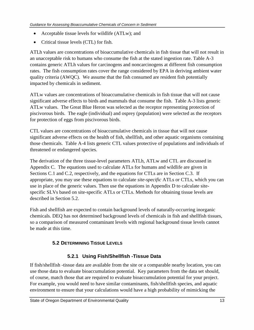
ATLh values are concentrations of bioaccumulative chemicals in fish tissue that will not result in
an unacceptable risk to humans who consume the fish at the stated ingestion rate. Table A-3
contains generic ATLh values for carcinogens and noncarcinogens at different fish consumption
rates. The fish consumption rates cover the range considered by EPA in deriving ambient water
quality criteria (AWQC). We assume that the fish consumed are resident fish potentially
impacted by chemicals in sediment.
ATLw values are concentrations of bioaccumulative chemicals in fish tissue that will not cause
significant adverse effects to birds and mammals that consume the fish. Table A-3 lists generic
ATLw values. The Great Blue Heron was selected as the receptor representing protection of
piscivorous birds. The eagle (individual) and osprey (population) were selected as the receptors
for protection of eggs from piscivorous birds.
CTL values are concentrations of bioaccumulative chemicals in tissue that will not cause
significant adverse effects on the health of fish, shellfish, and other aquatic organisms containing
those chemicals. Table A-4 lists generic CTL values protective of populations and individuals of
threatened or endangered species.
The derivation of the three tissue-level parameters ATLh, ATLw and CTL are discussed in
Appendix C. The equations used to calculate ATLs for humans and wildlife are given in
Sections C.1 and C.2, respectively, and the equations for CTLs are in Section C.3. If
appropriate, you may use these equations to calculate site-specific ATLs or CTLs, which you can
use in place of the generic values. Then use the equations in Appendix D to calculate site-
specific SLVs based on site-specific ATLs or CTLs. Methods for obtaining tissue levels are
described in Section 5.2.
Fish and shellfish are expected to contain background levels of naturally-occurring inorganic
chemicals. DEQ has not determined background levels of chemicals in fish and shellfish tissues,
so a comparison of measured contaminant levels with regional background tissue levels cannot
be made at this time.
5.2 DETERMINING TISSUE LEVELS
5.2.1 Using Fish/Shellfish -Tissue Data
If fish/shellfish -tissue data are available from the site or a comparable nearby location, you can
use those data to evaluate bioaccumulation potential. Key parameters from the data set should,
of course, match those that are required to evaluate bioaccumulation potential for your project.
For example, you would need to have similar contaminants, fish/shellfish species, and aquatic
environment to ensure that your calculations would have a high probability of mimicking the

Guidance for Assessing Bioaccumulative Chemicals of Concern in Sediment
State of Oregon Department of Environmental Quality 14
bioaccumulation that is occurring at the site. If appropriate fish/shellfish -tissue data are not
available, you can collect fish/shellfish from your site or use caged fish, mussels, or other in situ
caged animals for this purpose. In some cases caged mussels may be preferred since that test is
somewhat more standardized.
If you intend to use an exotic species such as fathead minnows or Corbicula in a caged test, you
should contact the Oregon Department of Fish and Wildlife and the US Fish and Wildlife Service
because you must not introduce exotic species into an area where they are not already present.
The home ranges of fish and other aquatic organisms collected at a site have uncertainties
associated with them. Conservative assumptions on home ranges, however, can still be used to
develop screening levels for evaluating a site. Although uncertainties in life history of species of
concern will exist for all ecological species, there are ways that uncertainty can be reduced
within the process, including the collection of fish and invertebrates with a smaller home range,
and that maintain a strong connection with the sediment. These species may include clams,
sculpin, or crayfish. Somewhat larger ranging, but localized fish such as smallmouth bass may
also be appropriate. The selection of localized species for site-specific evaluations will reduce
the uncertainty. During the development of the screening bioaccumulative values, it is assumed
that birds, mammals, and humans eat similar amounts of benthic invertebrates as they do fish and
that rates of bioaccumulation are similar. Total ingestion rates used to calculate ATLs are based
on fish but could be proportioned out for dietary preferences on a site-specific basis to adjust
ATLs for birds, mammals, and humans. Collection of benthic invertebrates and vertebrates help
to refine the exposure modeling. If you are considering this option, be sure to discuss this with
the DEQ project manager to ensure that appropriate aquatic species are collected and analyses
performed.
If fluoranthene and/or pyrene are COIs at your site, then sampling of tissue should consider a
range of invertebrates and vertebrates at your site to account for the difference in metabolic
capabilities. In addition, it may be necessary to conduct a literature search for an appropriate
bird TRVs for fluoranthene, as it was not available at the time of this guidance development.
Life expectancy of fish is also an important factor in selecting an appropriate candidate fish to
sample. For many bioaccumulative chemicals, the longer the life expectancy of the fish, the
greater potential for bioaccumulation. Life expectancy along with life history should be
considered in selecting relevant fish species to sample.
To evaluate the bioaccumulation potential, compare tissue data to the ATLh values in Table A-3,
the ATLw values in and Table A-4, and the CTL values in Table A-5. Use the 90UCL or the
maximum concentration, whichever is less, as the tissue concentration. Concentrations greater
than the table values indicate that bioaccumulation could be a threat to humans or wildlife that
consume aquatic organisms or to the organisms themselves.

Guidance for Assessing Bioaccumulative Chemicals of Concern in Sediment
State of Oregon Department of Environmental Quality 15
SUMMARY: If there are no COPCs on the basis of measured fish and/or shellfish tissue concentrations and ATLs or CTLs, no further action is required for bioaccumulation. If you identify one or more bioaccumulative COPCs as a result of the process described in Sub-section 5.2.1, you can either:
Carry out a response action for each COPC at the site as discussed in Section 6; or
If you think that chemicals in fish are not due to exposure to your site sediments, perform
controlled bioaccumulation tests, either in the lab or in situ, as described in Sub-
section 5.2.2. Use the fish/shellfish-tissue data from one or more of these tests to
determine if an unacceptable bioaccumulative risk is present.
5.2.2 Bioaccumulation Bioassays
If you decide to use bioaccumulation bioassays, the DEQ recommends that you use one or more
of the tests described in Appendix E. Questions about these tests or proposals for different tests
should be directed to the DEQ project manager.
If you use one of these tests, you can either assume that fish tissue concentrations equal the
invertebrate tissue concentrations, or use the invertebrate tissue concentrations in a food-web
model to estimate fish-tissue concentrations for the species of interest.
6. RESPONSE ACTIONS
6.1 IF A BIOACCUMULATOR IS DETECTED
After evaluating the options for assessing bioaccumulation that are previously described in this
document, if you have one or more chemicals that are bioaccumulators, and present or
potentially present unacceptable risk you will have to develop a response action to bring the risk
from these compounds down to acceptable levels.
A response action can be carried out by means of an engineering evaluation/cost analysis
(EE/CA) and a removal, or by a feasibility study (FS) and a remedial action depending on where
you are in the overall site evaluation and remediation process. Your target cleanup level would
be the generic SLV, the site-specific SLV, or ND, whichever is highest.
If you have information showing clearly that one or more of the BCOIs are present as a result of
area-wide contamination from other sources in addition to site-specific releases, you should
bring that information to the DEQ to discuss the need to develop a broader approach, potentially
on a watershed basis, for remedial action in the area. Examples 2 and 3 show how to determine
the baseline level of such contaminants depending upon the number of available data points.

Guidance for Assessing Bioaccumulative Chemicals of Concern in Sediment
State of Oregon Department of Environmental Quality 16
Note, however, that although it may not be feasible to remediate to below ambient levels, if these
concentrations exceed acceptable risk levels ambient concentrations will not be the final cleanup
levels for the site and additional remediation may be necessary in the future. A periodic review
of conditions will be required, typically on a five to ten year cycle.
Example 2
This example for determining ambient concentrations is for a site with at least 5, but less than 50,
upstream samples.
At Site A, 17 sediment samples are collected in the upstream area and the resulting contaminant
concentrations are evaluated statistically to determine the 90UCL for each contaminant. The method
used for this calculation depends on the frequency of detection of each contaminant.
1. If the frequency of detection is greater than or equal to 85% and there are at least 9 samples,
calculate the 90th percentile of the data as follows:
a. First, determine if the data are normally or log normally distributed using a standard statistical test
such as Shapiro-Wilk or Kolmogorov-Smirnov.
b. Depending on the distribution of the data, calculate the 90th percentile of the data.
2. If the frequency of detection is greater than or equal to 85% and there are at least 5 samples but
less than 9 samples, calculate the 95th percentile of the data by using the interquartile (IQR) approach
as follows:
a. Arrange the data in numerical order from the lowest to the highest value and determine the median
of the data set.
b. Identify the datum that lies halfway between the median and the highest datum. This value is the
upper quartile. The datum that lies halfway between the median and the lowest datum is the lower
quartile. If there is an even number of samples in any group there will not be a single datum at the
halfway point. In that case, calculate the average of the two data points that are on each side of the
halfway point.
c. Calculate the IQR as the difference between the upper quartile and lower quartile.
d. Estimate the 95th percentile of the data as the median of the data set plus 2 times the IQR. Use
this estimate to approximate the 90th percentile of the data set.
3. If the frequency of detection is greater than or equal to 50% but less than 85% and there are at
least 5 samples, calculate the 90th percentile of the data by Cohen’s method as described in Case 2 of
the Supplement to Statistical Guidance for Ecology Site Managers (WDOE 1998).
4. If the frequency of detection is less than 50%, use the maximum detected value for the 90th
percentile of the data.
5. If all samples are non-detect, use the minimum repeatedly achieved reporting limit for the 90th
percentile of the data.
After using the appropriate method(s) to calculate the 90th percentile for the data set, the
ambient/baseline value for each chemical is the lesser of the 90th percentile and the maximum detected
concentration unless that value is less than the minimum repeatedly-achieved reporting limit, in which
case the minimum repeatedly-achieved reporting limit is used.

Guidance for Assessing Bioaccumulative Chemicals of Concern in Sediment
State of Oregon Department of Environmental Quality 17
Ambient/baseline values are not estimated for data sets with fewer than 5 samples.
The results of the analysis for site A are presented in Table F-1 in Appendix F.
Implications: Active cleanup areas are identified in sediment at the site through a combination of risk-
based levels and exceedances of ambient/baseline concentrations. In this case, because the ambient
concentrations were generally low, it was determined that this cleanup would be protective considering
what the residual site-wide concentrations would be, after the remedial action.
Example 3
This example is for a site with 50 or more data points in the water body both upstream and downstream
of the site.
A broad-scale sediment sampling effort is conducted in the water body impacted by Site B. This
includes the collection of approximately 300 sediment samples. The results are evaluated as follows:
1. Sort the concentration data by contaminant. Where a contaminant is not detected, use a value of
½ the analytical detection limit. If a detection limit is not reported by the laboratory, use 0.167 times the
analytical reporting limit because analytical reporting limits are typically about 3 times the analytical
detection limit. DEQ will also consider more sophisticated methods for addressing non-detect values.
2. List the results for each contaminant from lowest to highest concentration and plot them on a linear
graph (see Figure F-1 in Appendix F for an example with DDE data).
3. The intersection of the asymptote to the lower part of the curve with the y-axis on the right side of
the plot is considered to be the maximum baseline concentration.
For the DDE example in Figure F-1 the baseline value is 7 ppb.
Implications: Although the health-based screening criteria for DDE, considering the potential for bioaccumulation and associated food chain impacts, is 0.03 ppb, DEQ concluded that active cleanup of DDE at the site to concentrations below 7 ppb was not feasible. A remedial action objective for DDE was established at the baseline concentration of 7 ppb. Once cleanup to this concentration was achieved, DEQ issued a conditional No Further Action determination, which indicated that further active remediation was not required at the site at this time, but that a full NFA could not be provided until protective concentrations were achieved through a combination of implementation of watershed-wide source control actions by other parties and natural recovery. Periodic review of conditions will be required on ten year cycle.
6.2 IF NO BIOACCUMULATOR IS DETECTED
If no chemicals exceed ATLs or CTLs, then the risk assessment would conclude the
bioaccumulation pathway does not pose an unacceptable risk, and would similarly present
conclusions concerning the risk evaluation for toxicity, and risks associated with other media of
concern.

Guidance for Assessing Bioaccumulative Chemicals of Concern in Sediment
State of Oregon Department of Environmental Quality 18
6.3 COMPLIANCE MONITORING
After you complete the removal action or the remediation you will have to monitor the site to
confirm that the objective of reducing the availability of site-related contaminants to fish,
shellfish, and other aquatic prey animals has been achieved. This could include sediment
sampling, and/or biota sampling, if relevant. In cases where the sediment work has been part of
a larger project to improve a watershed, estimating the reduction in the overall contaminant load
may be another way to assess success.

Appendix A.
Tables for Bioaccumulation Screening

Guidance for Assessing Bioaccumulative Chemicals of Concern in Sediment
State of Oregon Department of Environmental Quality A-1
Table A-1
Table A-1a: Sediment Bioaccumulation Screening Level Values (SLVs)
Chemical CASRN Birds (a)
(mg/kg dry wt) Mammals (b) (mg/kg dry wt)
Fish (mg/kg dry wt)
Humans (c) (mg/kg dry wt)
Inorganic Background (mg/kg dry wt.)
Individual (d) Population (e) Individual (d) Population (e) Freshwater Marine General (f) Subsistence
(g) Freshwater
Arsenic 7440-38-2 (h) (h) (h) (h) (h) (h) (h) (h) 7
Cadmium 7440-43-9 (h) (h) (h) (h) (h) (h) (h) (h) 1
Chlordane 12789-03-6 0.010 0.051 0.028 0.056 0.00050 0.00047 0.00037 4.6E-5 NA
DDT (Total) NA 0.00043 9.5E-5 (i)
0.0013 0.00034 (i)
0.0049 0.024 0.00039 0.00039 0.00033 (j) 4.0E-5 (j) NA
Dieldrin 60-57-1 0.00037 0.0018 0.0012 0.0061 0.0022 0.0022 8.1E-6 1.0E-6 NA
Dioxin / Furan Congeners NA Table A-1b Table A-1b Table A-1b Table A-1b NA
Fluoranthene 206-44-0 NA NA 360 1,800 37 37 510 62 NA
Hexachlorobenzene 118-74-1 NA NA NA NA 61 61 0.019 0.0023 NA
Lead 7439-92-1 (h) (h) (h) (h) (h) (h) (h) (h) 17
Mercury (measured as
total inorganic mercury) 7439-97-6 (h) (k) (h) (k) (h) (k) (h) (k) (h) (h) (h) (h) 0.07
Pentachlorophenol 87-86-5 NA NA 0.33 3.3 0.31 0.17 0.25 0.030 NA
PCB Congeners NA Table A-1b Table A-1b Table A-1b Table A-1b Table A-1b Table A-1b Table A-1b Table A-1b NA
PCBs (total as Aroclors) Bird egg
NA 0.057
0.0018 (i) 0.17
0.091 (i) 0.044 0.084 0.022 0.047 0.00039 4.8E-5 NA
Pyrene 129-00-0 NA NA 18,000 90,000 1.9 1.9 380 47 NA
Selenium 7782-49-2 (h) (h) (h) (h) (h) (h) (h) (h) 2
2,3,7,8-TCDD Bird egg
7.0E-7
1.7E-6 (i) 3.5E-6
3.5E-6 (i) 5.2E-8 1.4E-6 5.6E-7 5.6E-7 9.1E-9 1.1E-9 NA
Tributyltin 56-35-9 1.6 4.1 0.73 1.1 0.0023 0.00037 0.085 0.010 NA
NA = not applicable or not available Footnotes follow Table A-1b below

Guidance for Assessing Bioaccumulative Chemicals of Concern in Sediment
State of Oregon Department of Environmental Quality A-2
Table A-1b: SLVs for Designated Dioxin/Furan and PCB Congeners
CHEMICAL CASRN Birds (a)
(mg/kg dry wt) Mammals (b)
(mg/ dry wt) Fish
(mg/kg dry wt) Humans (c) (mg/kg dry wt)
Individual (d) Population (e) Individual (d) Population (e) Freshwater Marine General Subsistence
Dioxin/Furan Congeners
2,3,7,8-TCDD 7.0E-7
1.7E-6 (i) 3.5E-6
3.5E-6 (i) 5.2E-8 1.4E-6 5.6E-7 5.6E-7 9.1E-9 1.1E-9
1,2,3,7,8-PeCDD 2.1E-5 1.1E-4 1.5E-6 4.2E-5 1.7E-5 1.7E-5 2.7E-7 3.4E-8
1,2,3,4,7,8-HxCDD 4.2E-4 2.1E-3 1.5E-5 4.2E-4 3.4E-5 3.4E-5 2.7E-6 3.4E-7
1,2,3,6,7,8-HxCDD 2.1E-3 1.1E-2 1.5E-5 4.2E-4 1.7E-3 1.7E-3 2.7E-6 3.4E-7
1,2,3,7,8,9-HxCDD 2.1E-4 1.1E-3 1.5E-5 4.2E-4 1.7E-3 1.7E-3 2.7E-6 3.4E-7
1,2,3,4,6,7,8-HpCDD 5.3E-1 2.7E+0 3.9E-3 1.1E-1 4.3E-1 4.3E-1 6.9E-4 8.5E-5
OCDD 5.3E+0 2.7E+1 1.3E-1 3.6E+0 4.3E+0 4.3E+0 2.3E-2 2.8E-3
2,3,7,8-TCDF 5.9E-6 3.0E-5 4.3E-6 1.2E-4 9.5E-5 9.5E-5 7.7E-7 9.4E-8
1,2,3,7,8-PeCDF 5.9E-5 3.0E-4 1.4E-5 4.0E-4 9.5E-5 9.5E-5 2.6E-6 3.1E-7
2,3,4,7,8-PeCDF 7.0E-7 3.5E-6 1.7E-7 4.7E-6 1.1E-6 1.1E-6 3.0E-8 3.7E-9
1,2,3,4,7,8-HxCDF 2.1E-4 1.1E-3 1.5E-5 4.2E-4 1.7E-4 1.7E-4 2.7E-6 3.4E-7
1,2,3,6,7,8-HxCDF 2.1E-4 1.1E-3 1.5E-5 4.2E-4 1.7E-4 1.7E-4 2.7E-6 3.4E-7
2,3,4,6,7,8-HxCDF 2.1E-4 1.1E-3 1.5E-5 4.2E-4 1.7E-4 1.7E-4 2.7E-6 3.4E-7
1,2,3,7,8,9-HxCDF 2.1E-4 1.1E-3 1.5E-5 4.2E-4 1.7E-4 1.7E-4 2.7E-6 3.4E-7
1,2,3,4,6,7,8-HpCDF 5.3E-2 2.7E-1 3.9E-3 1.1E-1 4.3E-2 4.3E-2 6.9E-4 8.5E-5
1,2,3,4,7,8,9-HpCDF 5.3E-2 2.7E-1 3.9E-3 1.1E-1 4.3E-2 4.3E-2 6.9E-4 8.5E-5
OCDF 5.3E+0 2.7E+1 1.3E-1 3.6E+0 4.3E+0 4.3E+0 2.3E-2 2.8E-3
PCB Congeners (m)
3,3',4,4'-TCB PCB 77 8.0E-6 4.0E-5 3.0E-4 8.1E-3 3.2E-3 3.2E-3 5.2E-5 6.4E-6
3,4,4',5-TCB PCB 81 4.0E-6 2.0E-5 9.8E-5 2.7E-3 6.5E-4 6.5E-4 1.7E-5 2.1E-6
2,3,3',4,4'-PeCB PCB 105 3.9E-3 1.9E-2 9.4E-4 2.6E-2 6.2E-2 6.2E-2 1.7E-4 2.1E-5
2,3,4,4',5-PeCB PCB 114 4.0E-2 2.0E-1 9.8E-4 2.7E-2 6.5E-2 6.5E-2 1.7E-4 2.1E-5
2,3',4,4',5-PeCB PCB 118 4.9E-2 2.4E-1 1.2E-3 3.3E-2 7.9E-2 7.9E-2 1.2E-4 2.6E-5
2',3,4,4',5-PeCB PCB 123 4.9E-2 2.4E-1 1.2E-3 3.3E-2 7.9E-2 7.9E-2 2.1E-4 2.6E-5

Guidance for Assessing Bioaccumulative Chemicals of Concern in Sediment
State of Oregon Department of Environmental Quality A-3
3,3',4,4',5-PeCB PCB 126 3.9E-6 1.9E-5 2.8E-7 7.8E-6 6.2E-5 6.2E-5 5.0E-8 6.2E-9
2,3,3',4,4',5'-HxCB PCB 156 4.9E-3 2.4E-2 1.2E-3 3.3E-2 7.9E-2 7.9E-2 2.1E-4 2.6E-5
2,3,3',4,4',5-HxCB PCB 157 4.9E-3 2.4E-2 1.2E-3 3.3E-2 7.9E-2 7.9E-2 2.1E-4 2.6E-5
2,3',4,4',5,5'-HxCB PCB 167 4.9E-2 2.4E-1 1.2E-3 3.3E-2 7.9E-2 7.9E-2 2.1E-4 2.6E-5
3,3',4,4',5,5'-HxCB PCB 169 4.9E-4 2.4E-3 1.2E-6 3.3E-5 7.9E-2 7.9E-2 2.1E-7 2.1E-8
2,3,3',4,4',5,5'-HpCB PCB 189 2.7E-1 1.4E-0 6.6E-3 1.8E-1 4.3E-1 4.3E-1 1.2E-3 1.4E-4
Notes for Table A-1:
Values represented from food web model going from sediment to fish and then to piscivorous birds, mammals, and humans. See Appendix D for the SLV development methodology.
(a) The Great Blue Heron was the selected receptor for protection of piscivorous birds. The eagle (individual) and the osprey (population) were the selected receptors for protection of eggs from piscivorous birds.
(b) Mink was the selected piscivorous mammal receptor. (c) Calculated from SLV = foc x ATL / (BSAF x fL) where ATL is the acceptable tissue level for humans. See Table A-3. (d) Based on individual ATLs derived from a no observed adverse effects level (NOAEL). See Table A-3. (e) Based on population ATLs derived from a low observed adverse effects level (LOAEL). See Table A-3. (f) Based on general/recreational fish ingestion rate of 0.0175 kg/day. (g) Based on subsistence/ tribal fish ingestion rate of 0.1424 kg/day. (h) Screen using either site specific or default regional background concentrations (shown in the column on the right in this table). (i) Value represents the safe level for bird egg development based on methodology in Appendix C. SLV listed for DDT is protective of bird egg
development for DDE. (j) Value for DDE. (k) Sites with mercury contamination should collect actual fish tissue data at the site. Site-specific conditions regulate the methylization process form
sediment or water into aquatic receptors. (l) Based on CTLs (Table A-4). (m) The presentation of SLVs for dioxin-like PCB congeners does not imply that analysis of PCB congeners in sediment samples will be required. Analysis
of PCB congeners in fish and shellfish (see Table A-3a) is usually more relevant. However, if analysis of PCB congeners is performed in sediment, the SLVs can be used as screening values.

Guidance for Assessing Bioaccumulative Chemicals of Concern in Sediment
State of Oregon Department of Environmental Quality A-4
Table A-2.
Table A-2a: Exposure Parameters Used to Calculate Screening Level Values
Parameter Units Description Value
ATLhC mg/kg Acceptable carcinogen tissue level Calculated
ATLhN mg/kg Acceptable noncarcinogen tissue level Calculated
ARLC unitless Acceptable risk level for carcinogens 1 x 10⁻⁶
ARLN unitless Acceptable risk level for non-carcinogens 1
AT Years Averaging time 70
ED Years Exposure duration 30
SFo (mg/kg/day)-1 Slope factor – oral See Table 2b
RfD mg/kg/day Reference dose See Table 2b
BW Kg Body weight – adult human 70
IRP Kg/day Ingestion rate of fish by humans (from EPA’s AWQC for general and subsistence)
Recreational & General = 0.0175
Subsistence & Tribal = 0.1424
SLVBH mg/kg Sediment bioaccumulation screening level for humans
Calculated
BSAF Kg-oc/Kg-lipid Biota-sediment accumulation factor for organics
See Table 6
foc Unitless Fraction of total organic carbon 0.01
fL Unitless Fraction of lipid content Humans = 0.03 Wildlife = 0.05
TRVW mg/kg/day Toxicity reference value for wildlife See Table 7
IRW Kg/day Ingestion rate (wet wt.) by wildlife Heron = 0.42 Mink = 0.137
BWW Kg Body weight – wildlife Heron = 2.39
Mink = 1
ATLW mg/kg Acceptable tissue level for wildlife See Table 3
ATLW-egg mg/kg Acceptable tissue level for bird eggs (Wiemeyer et al. 1993)
See Table 3
BMFegg Unitless Biomagnification factor – fish tissue to bird eggs (Henny 2003)
See Table 6
SLVBW mg/kg Sediment bioaccumulation SLV for fish-eating wildlife
Calculated
NA = not applicable or not available
Footnotes follow Table A-2b below

Guidance for Assessing Bioaccumulative Chemicals of Concern in Sediment
State of Oregon Department of Environmental Quality A-5
Table A-2b: Table: Human Toxicity Values Used to Calculate Screening Level Values
CHEMICAL CASRN
Slope Factor (a)
(mg/kg/day)-1
Reference Dose (a)
(mg/kg/day)
Arsenic 7440-38-2 1.5 0.0003
Cadmium 7440-43-9 NA 0.001
Chlordane 12789-03-6 0.35 0.0005
4,4’-DDD 72-54-8 0.24 0.0005
4,4’-DDE 72-55-9 0.34 0.0005
4,4’-DDT 50-29-3 0.34 0.0005
DDT (Total) NA 0.34(c) 0.0005
Dieldrin 60-57-1 16 0.00003
Dioxin and Furan Congeners
(as 2,3,7,8-TCDD TEQ) NA 1.5 x 10⁵ NA
Fluoranthene 206-44-0 NA 0.04
Hexachlorobenzene 118-74-1 1.6 0.0008
Lead 7439-92-1 (d) (d)
Mercury (measured as organic mercury) 7439-97-6 NA 0.0001
Pentachlorophenol 87-86-5 0.12 0.03
PCB Congeners
(as 2,3,7,8-TCDD TEQ) NA 1.5 x 10⁵ NA
PCBs (total as Aroclors) NA 2 0.00002
Pyrene 129-00-0 NA 0.03
Selenium 7782-49-2 NA 0.005
Tributyltin 56-35-9 NA 0.0003
Notes for Table A-2
(a) Source: EPA’s Integrated Risk Information System (IRIS), 2006. (b) NA = not applicable. (c) Use the slope factor for 4,4’-DDE. (d) Slope factors and RfDs are not available for lead. In their study of the Columbia River Basin (USEPA 2002c), EPA used the Integrated Exposure Uptake Biokinetic (IEUBK) model and the Adult Lead Model (ALM) to calculate acceptable levels of lead in fish consumed by humans.

Guidance for Assessing Bioaccumulative Chemicals of Concern in Sediment
State of Oregon Department of Environmental Quality A-6
Table A-3
Table A-3a: Acceptable Tissue Levels (ATLs) for Chemicals in Fish/Shellfish Consumed by Wildlife and Humans
Wildlife Humans
Birds
(mg/kg wet wt.)
Mammals (mg/kg wet wt.)
Carcinogens (mg/kg wet wt.)
Non-carcinogens (mg/kg wet wt.)
CHEMICAL CASRN Individual (c) Population (d) Individual (c) Population (d) General /
Recreational (a) Subsistence / Tribal (b)
General / Recreational (a)
Subsistence / Tribal (b)
Arsenic 7440-38-2 13 64 7.6 38 0.0062 0.00076 1.2 0.15
Cadmium 7440-43-9 8.4 42 5.6 28 NA NA 4.0 0.49
Chlordane 12789-03-6 1.2 6.1 3.3 6.7 0.027 0.0033 2.0 0.25
DDT (Total) Bird egg
NA 0.051
0.013 (e,g,j) 0.15
0.048 (e,h,j) 0.58 2.9 0.027 0.0034 2.0 0.25
Dieldrin 60-57-1 0.044 0.22 0.15 0.73 0.00058 0.000072 0.12 0.015
Dioxin and Furan Congeners NA NA NA NA NA NA NA NA NA
Fluoranthene 206-44-0 NA NA 190 950 NA NA 160 20
Hexachlorobenzene 118-74-1 NA NA NA NA 0.0058 0.00072 3.2 0.39
Lead 7439-92-1 9.3 46 34 170 NA NA 0.5 (k) 0.5 (k)
Mercury (measured as total
inorganic mercury or methyl mercury)
7439-97-6 0.074
0.18 (f) 0.15
0.89 (f) 0.12 0.20 NA NA 0.40 0.049
Pentachlorophenol 87-86-5 NA NA 0.18 1.8 0.078 0.0096 120 15
PCB Congeners NA NA NA NA NA NA NA NA NA
PCBs (total as Aroclors) (i) NA 1.1
0.035 (e,g) 3.4
1.8 (e,h) 0.88 1.7 0.0047 0.00057 0.08 0.0098
Pyrene 129-00-0 NA NA 9,500 47,000 NA NA 120 15
Selenium 7782-49-2 0.23 0.46 0.036 0.88 NA NA 20 2.5
TCDD, 2,3,7,8-, TEQ Bird egg
NA 8.0E-6
1.9E-5 (e,g) 4.0E-5
4.0E-5 (e,h) 5.8E-7 1.6E-5 6.2E-8 7.6E-9 NA NA
Tributyltin 56-35-9 39 96 17 26 NA NA 1.2 0.15
Guidance for Assessing Bioaccumulative Chemicals of Concern in Sediment
State of Oregon Department of Environmental Quality A-7
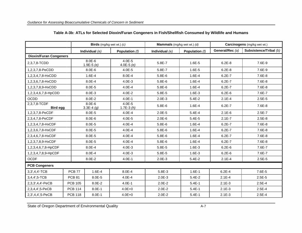
Table A-3b: ATLs for Selected Dioxin/Furan Congeners in Fish/Shellfish Consumed by Wildlife and Humans
PCB Congeners
3,3',4,4'-TCB PCB 77 1.6E-4 8.0E-4 5.8E-3 1.6E-1 6.2E-4 7.6E-5
3,4,4',5-TCB PCB 81 8.0E-5 4.0E-4 2.0E-3 5.4E-2 2.1E-4 2.5E-5
2,3,3',4,4'-PeCB PCB 105 8.0E-2 4.0E-1 2.0E-2 5.4E-1 2.1E-3 2.5E-4
2,3,4,4',5-PeCB PCB 114 8.0E-1 4.0E+0 2.0E-2 5.4E-1 2.1E-3 2.5E-4
2,3',4,4',5-PeCB PCB 118 8.0E-1 4.0E+0 2.0E-2 5.4E-1 2.1E-3 2.5E-4
Birds (mg/kg wet wt.) (c) Mammals (mg/kg wet wt.) (d) Carcinogens (mg/kg wet wt.)
Individual (e) Population (f) Individual (e) Population (f) General/Rec (a) Subsistence/Tribal (b)
Dioxin/Furan Congeners
2,3,7,8-TCDD 8.0E-6
1.9E-5 (e) 4.0E-5
4.0E-5 (e) 5.8E-7 1.6E-5 6.2E-8 7.6E-9
1,2,3,7,8-PeCDD 8.0E-6 4.0E-5 5.8E-7 1.6E-5 6.2E-8 7.6E-9
1,2,3,4,7,8-HxCDD 1.6E-4 8.0E-4 5.8E-6 1.6E-4 6.2E-7 7.6E-8
1,2,3,6,7,8-HxCDD 8.0E-4 4.0E-3 5.8E-6 1.6E-4 6.2E-7 7.6E-8
1,2,3,7,8,9-HxCDD 8.0E-5 4.0E-4 5.8E-6 1.6E-4 6.2E-7 7.6E-8
1,2,3,4,6,7,8-HpCDD 8.0E-3 4.0E-2 5.8E-5 1.6E-3 6.2E-6 7.6E-7
OCDD 8.0E-2 4.0E-1 2.0E-3 5.4E-2 2.1E-4 2.5E-5
2,3,7,8-TCDF Bird egg
8.0E-6
3.3E-4 (g) 4.0E-5
1.7E-3 (h) 5.8E-6 1.6E-4 6.2E-7 7.6E-8
1,2,3,7,8-PeCDF 8.0E-5 4.0E-4 2.0E-5 5.4E-4 2.1E-6 2.5E-7
2,3,4,7,8-PeCDF 8.0E-6 4.0E-5 2.0E-6 5.4E-5 2.1E-7 2.5E-8
1,2,3,4,7,8-HxCDF 8.0E-5 4.0E-4 5.8E-6 1.6E-4 6.2E-7 7.6E-8
1,2,3,6,7,8-HxCDF 8.0E-5 4.0E-4 5.8E-6 1.6E-4 6.2E-7 7.6E-8
2,3,4,6,7,8-HxCDF 8.0E-5 4.0E-4 5.8E-6 1.6E-4 6.2E-7 7.6E-8
1,2,3,7,8,9-HxCDF 8.0E-5 4.0E-4 5.8E-6 1.6E-4 6.2E-7 7.6E-8
1,2,3,4,6,7,8-HpCDF 8.0E-4 4.0E-3 5.8E-5 1.6E-3 6.2E-6 7.6E-7
1,2,3,4,7,8,9-HpCDF 8.0E-4 4.0E-3 5.8E-5 1.6E-3 6.2E-6 7.6E-7
OCDF 8.0E-2 4.0E-1 2.0E-3 5.4E-2 2.1E-4 2.5E-5

Guidance for Assessing Bioaccumulative Chemicals of Concern in Sediment
State of Oregon Department of Environmental Quality A-8
2',3,4,4',5-PeCB PCB 123 8.0E-1 4.0E+0 2.0E-2 5.4E-1 2.1E-3 2.5E-4
3,3',4,4',5-PeCB PCB 126 8.0E-5 4.0E-4 5.8E-6 1.6E-4 6.2E-7 7.6E-8
2,3,3',4,4',5'-HxCB PCB 156 8.0E-2 4.0E-1 2.0E-2 5.4E-1 2.1E-3 2.5E-4
2,3,3',4,4',5-HxCB PCB 157 8.0E-2 4.0E-1 2.0E-2 5.4E-1 2.1E-3 2.5E-4
2,3',4,4',5,5'-HxCB PCB 167 8.0E-1 4.0E+0 2.0E-2 5.4E-1 2.1E-3 2.5E-4
3,3',4,4',5,5'-HxCB PCB 169 8.0E-3 4.0E-2 2.0E-5 5.4E-4 2.1E-6 2.5E-7
2,3,3',4,4',5,5'-HpCB PCB 189 8.0E-1 4.0E+0 2.0E-2 5.4E-1 2.1E-3 2.5E-4
Notes for Table A-3:
(a) Based on a fish ingestion rate of 0.0175 kg/day. (b) (b) Based on a fish ingestion rate of 0.1424 kg/day. (c) The Great Blue Heron was the selected receptor for protection of piscivorous birds. The eagle (individual) and the osprey (population) were the
selected receptor for protection of eggs from piscivorous birds. (d) Mink was the selected piscivorous mammal receptor. (e) Individual ATLs are derived from a no adverse effects level. (f) Population ATLs are derived from a low adverse effects level. (g) Value represents safe level for eagle (individual) egg development based on methodology in Appendix C. Applies only to osprey or eagle receptors. (h) Value represents safe level for osprey (population) egg development based on methodology in Appendix C. Applies only to osprey or eagle receptors. (i) Ecological SLVs based on Aroclor 1254. (j) Osprey egg value is based on DDE because it is more toxic to bird-egg development than DDT. (k) Value taken from Columbia River Basin (USEPA 2002c)

Guidance for Assessing Bioaccumulative Chemicals of Concern in Sediment
State of Oregon Department of Environmental Quality A-9
Table A-4
Table A-4: CTLs for Chemicals in Fish, Shellfish, and Other Aquatic Organisms
Freshwater Marine
CHEMICAL CASRN Recommended
BCF (c) (l/Kg)
National Recommended WQC (a) (µg/l)
CTL (mg/kg)
wet weight
National Recommended WQC (a) (µg/l)
CTL (mg/kg)
wet weight Note
Arsenic 7440-38-2 44 150 6.6 36 1.6 (a)
Cadmium 7440-43-9 64 0.25 0.15 8.8 0.15 (b)(e)
Chlordane 57-74-9 14,000 0.0043 0.06 0.004 0.056 (d)
4,4'-DDT 50-29-3 54,000 0.001 0.054 0.001 0.054 (d)
4,4'-DDE 72-55-9 54,000 0.001 0.054 0.001 0.054 (d)
4,4'-DDD 72-54-8 54,000 0.001 0.054 0.001 0.054 (d)
Dieldrin 60-57-1 4700 0.056 0.26 0.056 0.26 (d)
Lead 7439-92-1 49 2.5 0.12 8.1 0.40 (b) (d)
Pentachlorophenol 87-86-5 11 15 0.17 7.9 0.087 (d)
PCBs (Total as Aroclors) 1336-36-3 31,000 0.014 0.43 0.03 0.93 (d)
PCB Congeners (see 2,3,7,8-TCDD TEQs)
(f) (f) (f) (f) (f) (f) (f)
Pyrene 129-00-0 30 300 (g) 1.0 300 (g) 1.0 (d) (g)
Selenium 7782-49-2 4.8 5.0 0.024 71 0.34 (d)
Tributyltin 56573-85-4 866 0.063 0.055 0.010 0.0087 (d)
Dioxins and Furan Congeners (as 2,3,7,8-TCDD TEQs)
1746-01-6 (f) (f) 6.4E-6 (f) 6.4E-6 (e)
Fluoranthene 206-44-0 1200 16 19 16 19 (d) (g)
Hexachlorobenzene 118-74-1 8700 3.68 32 3.68 32 (d) (g)
Mercury, inorganic (mercuric chloride)
33631-63-9 7,342 0.012 0.088 0.025 0.18 (d)
Mercury, organic (methyl mercury)
22967-92-6 (f) (f) (f) (f) (f) (f)
Notes for Table A-4:
(a) National Recommended Water Quality Criteria (WQC) (USEPA, 2004). (b) Cadmium and lead criteria are hardness dependent and were calculated using a hardness of 100
milligrams per liter. (c) See Appendix C for a discussion on how the recommended bioconcentration factor (BCF) was chosen. (d) The recommended tissue screening levels were calculated by multiplying the National Recommended
Water Quality Criteria by the recommended BCFs (e) See Appendix C for discussion on how species sensitivity distributions values were calculated. Values
presented are based on a species protection level of 95%. (f) Not available or not applicable. (g) WQC developed by USEPA are not available for these chemicals. DEQ developed their own values, as
presented in Appendix C. Pyrene value includes an adjustment using an acute/chronic ratio of 9.

Guidance for Assessing Bioaccumulative Chemicals of Concern in Sediment
State of Oregon Department of Environmental Quality A-10
Table A-5
Table A-5a: Default Uptake Values for Estimating Concentrations in Fish Tissue
CHEMICAL CASRN Kd
(unitless)
Log10 Kow
(unitless) (a)
Biota-Sediment Accumulation Factor (BSAF)
(kg oc/kg lipid) (b)
BMFegg
Eagle
(c)
BMFegg
Osprey
(d)
Arsenic 7440-38-2 29 NA NA NA NA
Cadmium 7440-43-9 6.7 NA NA NA NA
Chlordane 12789-03-6 NA 6.32 24 NA NA
4,4’-DDD 72-54-8 NA 6.10 24 NA NA
4,4’-DDE 72-55-9 NA 6.76 28 75 87
4,4’-DDT 50-29-3 NA 6.53 24 NA NA
DDT (Total) NA NA NA 24 NA NA
Dieldrin 60-57-1 NA 5.37 24 NA NA
Dioxin and Furans
(as 2,3,7,8-TCDD) NA NA See Table A-5b See Table A-5b 16 10
Fluoranthene 206-44-0 NA 5.12 0.105 NA NA
Hexachlorobenzene 118-74-1 NA 5.89 0.105 NA NA
Lead 7439-92-1 900 NA NA NA NA
Mercury 7439-97-6 NA NA NA 2.8 2.8 (f)
Pentachlorophenol 87-86-5 NA 5.09 0.105 NA NA
PCBs (congeners as
2,3,7,8-TCDD TEQs) NA NA See Table A-5b See Table A-5b NA NA
PCBs (total as aroclors) 1336363 NA 4.53 - 6.79 (e) 4(h) 113 11
Pyrene 129-00-0 NA 5.11 0.105 NA NA
Selenium 7782-49-2 5 NA NA NA NA
Tributyltin (oxide) 56-35-9 NA 3.84 (e) 4.70 (g) NA NA
Notes for Table A-5a:
(a) Taken from EPA’s Soil Screening Guidance (USEPA 1996) except as noted. (b) (WDOH 1995), 75th percentile (except for tributyltin oxide). Developed using logKow values that may not
match values in USEPA 1996. (c) Used as representative of threatened and endangered species. Taken from Buck, 2004, Table 23. (d) Used a representative of non-threatened and endangered species. Taken from Henny et al., 2003, Table XI. (e) Oak Ridge National Laboratory, Risk Assessment Information System (http://rais.ornl.gov/), May 2006. (f) BMF is for bald eagle eggs because osprey data are not available. (g) Linear interpolation of USACE 2007 data. Only invertebrate data are available. (h) Value for Aroclors 1242, 1248, and 1254 taken as representative of most PCB Aroclors in sediment.
Rounded from 3.962 (WDOH 1995).

Guidance for Assessing Bioaccumulative Chemicals of Concern in Sediment
State of Oregon Department of Environmental Quality A-11
Table A-5b: Default Uptake Values for Values for Designated Congeners
CHEMICAL
logKow
(b)
Toxic Equivalency Factor (TEF)
(unit less) (a) Biota-Sediment
Accumulation Factor (BSAF) (b)
(kg oc/kg lipid) Bird Fish Mammal and
Human
Dioxin/Furan Congeners
2,3,7,8-TCDD 7.02 1 1 1 2.268
1,2,3,7,8-PeCDD 7.5 1 1 1 0.076
1,2,3,4,7,8-HxCDD 7.8 0.05 0.5 0.1 0.076
1,2,3,6,7,8-HxCDD 7.8 0.01 0.01 0.1 0.076
1,2,3,7,8,9-HxCDD 7.8 0.1 0.01 0.1 0.076
1,2,3,4,6,7,8-HpCDD 8.2 <0.001 0.001 0.01 0.003
OCDD 8.6 0.0001 <0.0001 0.0003 0.003
2,3,7,8-TCDF 5.8 1 0.05 0.1 0.27
1,2,3,7,8-PeCDF 6.5 0.1 0.05 0.03 0.27
2,3,4,7,8-PeCDF 7 1 0.5 0.3 2.268
1,2,3,4,7,8-HxCDF 7.5 0.1 0.1 0.1 0.076
1,2,3,6,7,8-HxCDF 7.5 0.1 0.1 0.1 0.076
2,3,4,6,7,8-HxCDF 7.5 0.1 0.1 0.1 0.076
1,2,3,7,8,9-HxCDF 7.5 0.1 0.1 0.1 0.076
1,2,3,4,6,7,8-HpCDF 8 0.01 0.01 0.01 0.003
1,2,3,4,7,8,9-HpCDF 8 0.01 0.01 0.01 0.003
OCDF 8.8 0.0001 <0.0001 0.0003 0.003
PCB Congeners
3,3',4,4'-TCB PCB 77 0.05 0.0001 0.0001 3.962
3,4,4',5-TCB PCB 81 0.1 0.0005 0.0003 3.962
2,3,3',4,4'-PeCB PCB 105 <0.000005 0.00003 4.134
2,3,4,4',5-PeCB PCB 114 <0.000005 0.00003 3.962
2,3',4,4',5-PeCB PCB 118 <0.000005 0.00003 3.26
2',3,4,4',5-PeCB PCB 123 <0.000005 0.00003 3.26
3,3',4,4',5-PeCB PCB 126 0.1 0.005 0.1 4.134
2,3,3',4,4',5'-HxCB PCB 156 <0.000005 0.00003 3.26
2,3,3',4,4',5-HxCB PCB 157 <0.000005 0.00003 3.26
2,3',4,4',5,5'-HxCB PCB 167 <0.000005 0.00003 3.26
3,3',4,4',5,5'-HxCB PCB 169 0.001 <0.000005 0.03 3.26
2,3,3',4,4',5,5'-HpCB PCB 189 <0.000005 0.00003 0.59
Notes for Table A-5b:
(a) Van den Berg et al., 1998 and 2006.
(b) WDOH 1995. The BSAF is based on the 75th percentile (WDOH 1995). LogKow values for Aroclors ranged from 5.88 to 6.91.

Guidance for Assessing Bioaccumulative Chemicals of Concern in Sediment
State of Oregon Department of Environmental Quality A-12
Table A-6.
Table A-6a: Table: Toxicity Reference Values (TRVs)
CHEMICAL CASRN Birds (mg/kg/day) Mammals (mg/kg/day)
Individual Population Individual Population
Arsenic 7440-38-2 2.24 (a) 11.2 (a) (b) 1.04 (a) 5.2 (a) (b)
Cadmium 7440-43-9 1.47 (a) 7.35 (a) (b) 0.77 (a) 3.85 (a) (b)
Chlordane 12789-03-6 0.214 (c) (d) 1.07 (c) (d) 0.458 (c) (d) 0.915 (c) (d)
DDT (Total) NA 0.009 (e) (f) 0.027 (e) 0.08 (c) (e) (d) 0.4 (c) (e) (b)
Bird egg NA 1 (g) 4.2 (h) NA NA NA NA
Dieldrin 60-57-1 0.0077 (d) 0.039 (i) (d) 0.02 (d) 0.1 (d)
Dioxin/Furan Congeners
(as 2,3,7,8-TCDD TEQs) NA 1.4E-06 (e) 7E-06 (e) 8.0E-08 (j) 2.2E-06 (j)
Bird egg NA 0.00030 (k) 0.00040 (g) (l) NA NA NA NA
Fluoranthene 206-44-0 NA NA NA NA 26 (m) (n) 130 (m) (b) (n)
Hexachlorobenzene 118-74-1 NA NA NA NA NA NA NA NA
Lead 7439-92-1 1.63 (a) (o) 8.5 (a) (b) 4.7 (a) 23.5 (a) (b)
Mercury (methyl) 7439-97-6 0.013 (a) 0.026 (a) 0.016 (e) 0.027 (e)
Bird egg 7439-97-6 0.5 (p) 2.5 (i) NA NA NA NA
Pentachlorophenol 87-86-5 NA NA NA NA 0.024 (c) (d) 0.24 (c) (d)
PCBs (total as
2,3,7,8-TCDD TEQs) NA 1.4E-06 (e) 7E-06 (e) 8.0E-08 (j) 2.2E-06 (j)
PCBs (as Aroclor 1254) NA 0.2 (e) 0.6 (e) 0.12 (q) 0.23 (q)
Bird egg NA 4 (r) 20 (s) (i) NA NA NA NA
Pyrene 129-00-0 NA NA NA NA 1,300 (m) (n) 6,500 (m) (b) (n)
Selenium 7782-49-2 0.04 (c) (d) 0.08 (c) (d) 0.005 (m) (d) 0.121 (m) (d)
Tributyltin 56-35-9 6.8 (c) 16.9 (c) 2.34 (c) (d) 3.5 (c) (d)
NA = not applicable or not available Footnotes follow Table A-6b below

Guidance for Assessing Bioaccumulative Chemicals of Concern in Sediment
State of Oregon Department of Environmental Quality A-13
Table A-6b: Toxicity Reference Values for Designated Congeners
CHEMICAL CASRN Birds (t)
(mg/kg/day) Mammals (t)
(mg/kg/day)
Individual Population Individual Population
Dioxin/Furan Congeners
2,3,7,8-TCDD 0.0000014 (e) 0.000007 (e) 0.00000008 (j) 0.0000022 (j)
1,2,3,7,8-PeCDD 0.0000014 0.000007 0.00000008 0.0000022
1,2,3,4,7,8-HxCDD 0.000028 0.00014 0.0000008 0.000022
1,2,3,6,7,8-HxCDD 0.00014 0.0007 0.0000008 0.000022
1,2,3,7,8,9-HxCDD 0.000014 0.00007 0.0000008 0.000022
1,2,3,4,6,7,8-HpCDD 0.0014 0.007 0.000008 0.00022
OCDD 0.014 0.07 0.000266667 0.0073333
2,3,7,8-TCDF 0.0000014 0.000007 0.0000008 0.000022
1,2,3,7,8-PeCDF 0.000014 0.00007 2.66667E-06 7.333E-05
2,3,4,7,8-PeCDF 0.0000014 0.000007 2.66667E-07 7.333E-06
1,2,3,4,7,8-HxCDF 0.000014 0.00007 0.0000008 0.000022
1,2,3,6,7,8-HxCDF 0.000014 0.00007 0.0000008 0.000022
2,3,4,6,7,8-HxCDF 0.000014 0.00007 0.0000008 0.000022
1,2,3,7,8,9-HxCDF 0.000014 0.00007 0.0000008 0.000022
1,2,3,4,6,7,8-HpCDF 0.00014 0.0007 0.000008 0.00022
1,2,3,4,7,8,9-HpCDF 0.00014 0.0007 0.000008 0.00022
OCDF 0.014 0.07 0.000266667 0.0073333
PCB Congeners (r)
3,3',4,4'-TCB PCB 77 0.000028 0.00014 0.0008 0.022
3,4,4',5-TCB PCB 81 0.000014 0.00007 0.000266667 0.0073333
2,3,3',4,4'-PeCB PCB 105 0.014 0.07 0.002666667 0.0733333
2,3,4,4',5-PeCB PCB 114 0.14 0.7 0.002666667 0.0733333
2,3',4,4',5-PeCB PCB 118 0.14 0.7 0.002666667 0.0733333
2',3,4,4',5-PeCB PCB 123 0.14 0.7 0.002666667 0.0733333
3,3',4,4',5-PeCB PCB 126 0.000014 0.00007 0.0000008 0.000022
2,3,3',4,4',5'-HxCB PCB 156 0.014 0.07 0.002666667 0.0733333
2,3,3',4,4',5-HxCB PCB 157 0.014 0.07 0.002666667 0.0733333
2,3',4,4',5,5'-HxCB PCB 167 0.14 0.7 0.002666667 0.0733333
3,3',4,4',5,5'-HxCB PCB 169 0.0014 0.007 2.66667E-06 7.33E-05
2,3,3',4,4',5,5'-HpCB PCB 189 0.14 0.7 0.002666667 0.0733333
Notes for Table A-6:
(a) TRV from USEPA 2006. (b) A LOAEL was extrapolated from a NOAEL by multiplying the NOAEL x 5. (c) Sample, B.W., Opresko, D.M., and Suter II, G.W. ,1996. (d) An interspecies uncertainty factor of 10 was used. (e) USEPA 1995.

Guidance for Assessing Bioaccumulative Chemicals of Concern in Sediment
State of Oregon Department of Environmental Quality A-14
(f) Extrapolated NOAEL/LOAELs were performed according to the recommended methodology in the reference. (g) Eagle NOAEL or LOAEL taken from Wiemeyer et al., 1984; Kubiak, T.J. and D.A. Best, 1991; Elliot, J.E. and M.L. Harris, 2001/2002. (h) DDE LOAEL for the osprey was taken from Wiemeyer et al., 1988. (i) Population (LOAEL) TRVs were extrapolated from an individual (NOAEL) TRV by multiplying the individual TRV x 5. (j) Tillitt, D. E., et al. 1996. (k) Bald Eagle NOAEL and osprey NOAEL and LOAEL taken from Elliot, J.E. and M.L Harris, 2001/2002; Elliot J.E. et al., 1996. (l) The eagle NOAEL or LOAEL was used as a surrogate for the osprey. (m) California Department of Toxic Substances Control, 2000. (n) Calculated Pyrene TRVs from Benzo(a)pyrene TRVs by applying a TEF of 0.001; calculated Fluoranthene TRVs from Benzo(a)pyrene TRVs by applying a TEF of 0.05. (o) A NOAEL was extrapolated from a LOAEL by multiplying the LOAEL by 0.1. (p) Mercury NOAEL taken from Wiemeyer et al., 1993. (q) Total PCB TRVs for mink taken from Millsap et al. 2004. (r) The PCB NOAEL for bald eagle was taken from Wiemeyer et al., 1984. (s) 20 mg/kg was also suggested by Elliot, J.E. and M.L. Harris, 2001/2002 for a LOAEL for bald eagles, confirming the relevancy of this number for an osprey LOAEL. (t) Calculated Dioxin/PCB Congener TRVs from 2,3,7,8 TCDD TRV by applying TEFs from Van den Berg et al., 1998 and 2006.

Guidance for Assessing Bioaccumulative Chemicals of Concern in Sediment
State of Oregon Department of Environmental Quality A-15
Table A-7
Table A-7: Analytical Methods and Reporting Limits
Notes for Table A-7:
(a) Method reporting limit (MRL) on a dry-weight basis. (b) Method reporting limit (MRL) on a wet-weight basis (c) Method reporting limits for PCBs may require sample extract concentration step and other
sample extract cleanup procedures.
CHEMICAL CASRN Analytical
Method
Method Reporting Limit
Sediment (a)
Method Reporting Limit
Tissue (b)
METALS
Arsenic 7440-38-2 6010C or 7060A 1.0 mg/Kg 100 µg/kg
Cadmium 7440-43-9 6010C or 7131A 1.0 mg/Kg 100 µg/kg
Lead 7439-92-1 6010C 1.0 mg/Kg 500 µg/kg
Mercury 7439-97-6 7471B 2.0 µg/Kg 10 µg/kg
Selenium 7782-49-2 6010C or 7740 2.0 – 10 mg/Kg 100 µg/kg
ORGANICS
Chlordane 12789-03-6 8081A 5.0 µg/Kg 2 µg/kg
4,4’-DDD 72-54-8 8081A 1.0 µg/Kg 2 µg/kg
4,4’-DDE 72-55-9 8081A 1.0 µg/Kg 2 µg/kg
4,4’-DDT 50-29-3 8081A 1.0 µg/Kg 2 µg/kg
Dieldrin 60-57-1 8081A 1.0 µg/Kg 2 µg/kg
Dioxin and Furans (as 2,3,7,8-TCDD TEQs)
NA 8280, 8290, or 1613B 1-5 ng/Kg 2 ng/kg (ppt)
Fluoranthene 206-44-0 8310 or 8270C 100 µg/Kg 100 µg/kg
Hexachlorobenzene 118-74-1 8081A 660 µg/Kg 100 µg/kg
Pentachlorophenol 87-86-5 8181A or 8270C 1.0 µg/Kg 600 µg/kg
PCBs (individual congeners) NA 8082 or 1668A 1-5 µg/Kg (c) 20 ng/kg (ppt)
PCBs (individual Aroclors) NA 8081A or 8082 1-10 µg/Kg (c) 1-10 µg/Kg (c)
Pyrene 129-00-0 8310 100 µg/Kg 100 µg/Kg
Tributyltin 56-35-9 130.00 (NOAA) 10 µg/Kg 10 µg/Kg

Appendix B.
Regional Default Background Concentrations
for Soil/Sediment

Guidance for Assessing Bioaccumulative Chemicals of Concern in Sediment
State of Oregon Department of Environmental Quality B-1
Regional Default Background Concentrations for Soil/Sediment
When selecting metal background levels for a specific site, the preference for a source of such values
is, in order: (1) those calculated from site-specific data (assuming the sampling and analysis were
adequate, etc.), (2) local default values (e.g., those for SW Oregon), and (3) the regional default values
for the Pacific Northwest listed in the table below. Background values are based on the 90th or 95th
percentile of regional soil data.
The regional default values given below can be used (1) to make an initial assessment of a site (before
site-specific data are available), (2) if local default values are unavailable, or (3) to check the credibility of
site-specific values. They are to be used at the discretion of the DEQ cleanup project manager, can be
ignored, and should not be seen as constituting a background "standard" or "criteria". Other sources of
background information can be researched from the references section listed in this Appendix.
To determine if site concentrations are greater than background, compare the 90 percent upper
confidence limit on the arithmetic mean, or the maximum concentration, whichever is less, to the
background value shown in Table B-1.
Table B-1: Oregon DEQ Suggested Default Background Concentrations for Inorganic
Contaminants in Soil/Sediment
CHEMICAL Soil/Sediment (mg/kg, dw)
Arsenic 7 (a)
Cadmium 1 (b)
Lead 17 (c)
Mercury 0.07 (d)
Selenium 2 (e)
Notes for Table B-1:
(a) State-wide 90th percentile value from WDOE (1994). 95th percentile British Columbia regional soil background estimate for As is 10 mg/kg (BCE, 1999).
(b) State-wide 90th percentile value from WDOE (1994).
(c) State-wide 90th percentile value for Washington (WDOE, 1994). United States geometric mean value is 16
mg/kg (Fuhrer, 1986; Table 7). Lead range in Oregon soils reported as 1.2 to 18 mg/kg (Fuhrer, 1989; Table 8).
(d) 95th percentile British Columbia regional soil background value (BCE, 1999).
(e) State-wide 90th percentile value from WDOE (1994). 95th percentile British Columbia regional soil background
estimate for As is 10 mg/kg (BCE, 1999).

Guidance for Assessing Bioaccumulative Chemicals of Concern in Sediment
State of Oregon Department of Environmental Quality B-2
References for Appendix B
The following guidance should be considered for developing estimates of background for soil or sediments:
1. BCE, 1999. Protocol for Contaminated Sites 4 - Determining Background Soil Quality. British Columbia
Ministry of Water, Land, and Air Protection. Victoria, British Columbia, Canada.
2. EPA, 2002a. Role of Background in the CERCLA Cleanup Program. OSWER 9285.6-07P. U.S. Environmental Protection Agency, Office of Solid Waste and Emergency Response, Washington DC.
3. EPA, 2002b. Guidance for Comparing Background and Chemical Concentrations in Soil for CERCLA Sites, Appendix B: Policy Considerations for the Application of Background Data in Risk Assessment and Remedy Selection. EPA 540/R-01/003, OSWER 9285.7-41. U.S. Environmental
Protection Agency, Office of Solid Waste and Emergency Response, Washington DC.
4. Fuhrer, G.J., 1986. Extractable Cadmium, Mercury, Copper, Lead, and Zinc in the Lower Columbia River Estuary, Oregon and Washington. Water Resources Investigations Report 86-4088. U.S.
Geological Survey, Portland, Oregon.
5. Fuhrer, G.J., 1989. Quality of Bottom Material and Elutriates in the Lower Willamette River, Portland Harbor, Oregon. Water Resources Investigations Report 89-4005. U.S. Geological Survey, Portland,
Oregon.
6. Fuhrer, G.J. and Horowitz, A.J., 1989. The Vertical Distribution of Selected Trace Metals and Organic Compounds in Bottom Materials of the Proposed Lower Columbia River Export Channel. Water
Resources Investigations Report 95-4294. U.S. Geological Survey, Portland, Oregon.
7. Fuhrer, G.J., Tanner, D.O., Morace, J.L., McKenzie, S.W., and Skach, K.A., 1996. Water Quality of the Lower Columbia River Basin: Analysis of Current and Historical Water-Quality Data through 1994.
Water Resources Investigations Report 95-4294. U.S. Geological Survey, Portland, Oregon.
8. MacCoy, D.E. and Black, R.W., 1998. Organic Compounds and Trace Elements in Freshwater Streambed Sediment and Fish from the Puget Sound Basin. USGS Fact Sheet 105-98. Puget Sound
Basin NAWQA Study, U.S. Geological Survey, Seattle, Washington. [wa.water.usgs.gov/pugt/fs.105-98.html]
9. Meador, J.P., Clark Jr., R.C., Robisch, P.A., Ernest, D.W., Landahl, J.T., Varanasi, U., Chan, S-L., and McCain, B.B., 1994. National Benthic Surveillance Project: Pacific Coast. Analyses of Elements in Sediment and Tissue Cycles I to V (1984-88). NOAA Technical Memorandum NMFS-NWFSC-16.
National Marine Fisheries Service, National Oceanic and Atmospheric Administration, Seattle, Washington.
10. Nagpal, N. K. and Howell, K., 2001. Water Quality Guidelines for Selenium, Technical Appendix. British
Columbia Ministry of Water, Land, and Air Protection. Victoria, British Columbia, Canada.
11. Nozaki, Y., 1997. A fresh look at element distribution in the North Pacific. EOS electronic supplement,
posted May 27, 1997. [www.agu.org/eos_elec/]
12. Quinby-Hunt, M.S. and Turekian, K.K., 1983. Distribution of elements in sea water. EOS, 64: 130-131.
13. Quinby-Hunt, M.S. and Wilde, P., 1986/87. Modeling of dissolved elements in sea water. Ocean Science
and Engineering, 11:3,4, p. 153-251.
14. Rickert, D.A., Kennedy, V.C., McKenzie, S.W., and Hines, W.G., 1977. A Synoptic Survey of Trace Metals in Bottom Sediments of the Willamette River, Oregon. Geological Survey Circular 715-F. U.S.
Geological Survey, Arlington, Virginia.
15. WDOE, 1994. Natural Background Soil Metal Concentrations in Washington State. Publication #94-
115. Washington Department of Ecology, Olympia, WA.

Appendix C.
Calculating Acceptable Tissue Levels
&
Critical Tissue Levels

Guidance for Assessing Bioaccumulative Chemicals of Concern in Sediment
State of Oregon Department of Environmental Quality C-1
C.1 Acceptable Tissue Levels for Humans
For human consumption, acceptable tissue levels for carcinogens (ATLhC) and noncarcinogens
(ATLhN) are back-calculated from acceptable risk levels in accordance with federal guidance for
establishing fish consumption limits and for conducting human health risk assessments (USEPA,
1989, 1997). Calculated ATLh values are provided for your use in Appendix A, Table A-3.
Separate levels were not calculated for men and women, as differences in consumption rates
relative to body weight are minor.
Acceptable fish tissue levels for humans are calculated using the following equations.
For carcinogens:
EDIRSF
ATBWARLATLh
PO
CC
[C-1]
and for noncarcinogens:
P
NN
IR
ARLBWRfDATLh
[C-2]
where:
ATLhC = Acceptable tissue level (carcinogen) in diet for human receptors (mg/kg);
ATLhN = Acceptable tissue level (noncarcinogen) in diet for human receptors (mg/kg);
ARLC = Acceptable risk level for carcinogens (unitless; 1 10-6);
ARLN = Acceptable risk level for noncarcinogens (unitless; 1);
AT = Averaging time (years);
ED = Exposure duration (years);
SFo = Oral slope factor (mg/kgd)-1;
RfD = Reference dose (mg/kgd);
BW = Body weight (kg); and
IRP = Fish and/or shellfish ingestion rate for the exposed population
(mean daily rate over a year in kg/day).
The default calculations of ATLh do not take into consideration (1) the feeding range of a fish
species relative to the area of sediment contaminated by releases from the site, or (2) the fraction
of total fish consumed by humans that comes from the site. These factors can be considered in a

Guidance for Assessing Bioaccumulative Chemicals of Concern in Sediment
State of Oregon Department of Environmental Quality C-2
site-specific ATLh calculation. If you are considering development of site specific ATLh values,
be sure to discuss them with the DEQ project manager and get approval prior to making them.
The ATL values in Table A-3 represent the maximum concentration of a given chemical in fish
tissue that will NOT:
1. Generate a risk greater than the maximum acceptable risk level (ARL) used for
carcinogens; or
2. Cause adverse noncarcinogenic health effects based on a lifetime of daily consumption at
an exposure scenario-specific ingestion rate (IR, see Table A-2).
Therefore, the ATLh values permit a specific population of humans to consume safely any
combination of fish and/or shellfish for an extended period, provided that the combined daily
consumption rate remains below the value of IR used to calculate ATLh.
EPA has not developed a slope factor or reference dose for lead. The absence of toxicity factors
makes evaluation of acceptable tissue levles difficult. EPA addressed this issue during the
evaluation of data from the Columbia River basin fish contamination survey (USEPA 2002(c)).
They modeled lead exposure using the Integrated Exposure Uptake Biokinetic (IEUBK) model
and the Adult Lead Model (ALM). These models take into account lead exposure from a variety
of sources (including site sources, and in this case dietary fish sources), and calculate blood lead
levels. EPA determined that at a lead concentration of 500 µg/kg in fish, there was a less than 5
percent chance that blood lead levels would exceed the acceptable level of 10 µg/dl in children.
EPA also found that a lead concentration of 700 µg/kg in fish tissue consumed by a mother
results in less than a 5 percent chance that blood lead levels in a fetus will exceed acceptable
levels. The calculations included high fish consumption rates typical of Columbia River tribes.
Based on these results using regional data, DEQ is using 500 µg/kg (= 0.5 mg/kg) as an
acceptable concentration of lead in fish tissue to protect humans. Given the uncertainties, this
value will be applied to both typical and higher fish ingestion rates.
C.2 Acceptable Tissue Levels for Wildlife
An acceptable tissue level for wildlife (ATLw) is the concentration of a contaminant that an
animal could consume in its prey that would result in a dose equal to a given toxicity reference
value (TRV) without harming the individual animal or the population. This assumes that the
animal receives no additional exposure to that contaminant through other environmental media.
Calculated ATLw values are provided for your use in Table A-3. An ATLw can be calculated
from a TRV for a chemical either at a lowest-observable-effect-level (LOAEL), as a surrogate
for populations, or a no-observable-effect-level (NOAEL), as a surrogate for individuals, by
assuming a receptor’s total diet contains that chemical concentration (Sample et al., 1996).

Guidance for Assessing Bioaccumulative Chemicals of Concern in Sediment
State of Oregon Department of Environmental Quality C-3
Values in the “Population” columns of Table A-3 for birds and mammals represent chemical
concentrations in sediment at and below which chemicals are not expected to accumulate in the
tissues of prey items (e.g., fish) above LOAEL-based acceptable levels. These values imply the
possibility of adverse effects in individuals within a local population but not to the local
population as a whole. When the chemical concentration in all food items is constant, the
relationship between dose and the concentration in food items can be represented by the
following equation:
BWIR
TRVATLw W [C-3]
where:
ATLW = Acceptable tissue level in diet for wildlife receptors (mg/kg, wet weight diet);
TRVW = Toxicity reference value for wildlife (mg/kgbody weight day, dry weight;
NOAEL-based for individuals, LOAEL-based for populations);
BW = Body weight (kg) (Heron = 2.39 kg and Mink = 1 kg); and
IR = Daily food ingestion rate (kg wet weight/day) (Heron = 0.42 kg/d and Mink =
0.137 kg/d).
Mink and great blue heron were chosen as representative fish-eating receptors for mammals and
birds, respectively. Osprey was chosen as the representative fish-eating bird species for the egg
pathway when evaluating risk to populations, and eagle was chosen to evaluate risk to
individuals of threatened and endangered species. Their diets were assumed to consist entirely
of fish. Toxicological information on bird and mammal responses to various chemicals was
based on a number of sources listed in Table A-7. Different wildlife species may be evaluated
when mink and great blue heron are not present or when other species are more appropriate.
Several extrapolations were made to complete the ATLs if the desired toxicity threshold was not
provided. NOAELs were extrapolated to LOAELs by multiplying the NOAEL by 5. LOAELs
were extrapolated to NOAELs by multiplying the LOAEL by 0.1. Additionally, dioxin/PCB
toxicity equivalency factors (TEFs) were based on Van den Berg (1998 and 2006).
The default calculations of ATLw do not take into consideration:
The entire feeding range of the mammal relative to the part of the range where fish can be found
that have been contaminated from sediment at the site, or
The fraction of the total fish consumed by the mammal that comes from the site.

Guidance for Assessing Bioaccumulative Chemicals of Concern in Sediment
State of Oregon Department of Environmental Quality C-4
In other words, the default area-use factor for mammals and birds is set at one. This includes the
assumption that the receptors are present year-round and that they obtain all of their food from
the specific habitat area. While this may not be true for all potential receptors, these assumptions
were used to ensure that the species that do meet the criteria are afforded adequate protection.
Both of these factors may be considered if a site-specific ATLw is calculated.
An ecological receptor is generally selected to represent a class of organisms. For this reason
you should use risk assessment parameters that represent the other organisms in the class and not
just the individual receptor. Values of ATLw should also consider this factor. The feeding range
of a particular ecoreceptor may not be confined to the site in question but another member of the
same receptor class may use the entire site. The receptor classes could also be changed if the
ones that were used to calculate the generic ATLw values are not appropriate for the site. If you
are considering making changes, be sure to discuss them with the DEQ project manager and get
approval prior to making them.
When data are available for higher trophic level species, they should be incorporated into a food
web model or ecological risk assessment. Although these species generally have greater ranges
than the area within smaller cleanup sites, their addition can greatly improve confidence in a
food web model or when estimating risk. These are often the organisms we are trying to protect,
especially in cases where contaminants bioaccumulate in organisms lower in the food chain but
not to levels that adversely affect them.
For some chemicals, such as PCBs, DDTs, chlorinated dibenzo-p-dioxins and chlorinated
dibenzofurans, the most important and most sensitive effects on birds are to the developing
embryos. In this case, an ATLw-egg (in mg-chemical/kg-egg) is developed using NOAELs or
LOAELs available from EPA or other sources (e.g., US EPA, April 2003; Henny 2003; and
Buck 2004). ATLs for bird eggs are calculated with the following equation:
egg
w
eggWBMF
TRVATL [C-4]
where:
ATLW-egg = Acceptable tissue level in fish for protection of eggs of fish-eating birds
(mg/kg);
TRVw = Toxicity reference value for bird egg (mg/kg; NOAEL-based for individual eagles,
LOAEL-based for osprey populations) (Table A-6).
BMFegg = Biomagnification factor, fish tissue to bird eggs (Table A-5).

Guidance for Assessing Bioaccumulative Chemicals of Concern in Sediment
State of Oregon Department of Environmental Quality C-5
C.3 Critical Tissue Levels for Fish
Critical tissue levels (CTLs) represent concentrations in tissue at or below which approximately
95 percent of aquatic organisms bearing this residue would be highly unlikely (less than 5
percent chance) to experience adverse health effects. A CTL is one tool for evaluating the risk to
aquatic organisms from internal exposure to chemicals capable of bioaccumulation or
biomagnification. A CTL is not species specific, as benthic and pelagic biota appear to have
similar sensitivity to tissue residues, and should therefore meet the protectiveness standard (i.e.,
avoidance of “significant adverse impacts”) under ORS 465.315, and the administrative rules
promulgated thereto, for a variety of aquatic ecological receptors.
The two methods used to derive CTLs are presented below.
The ambient water quality criteria and bioconcentration factor method (AWQC x BCF
Method) from Shephard, et al. (1998); and
The species sensitivity distribution method (SSD method), which employs empirical-
effects data.
Table C-1, below, summarizes the two databases that were used to select no-observed-effects
residue and lowest-observed-effects residue (NOER/LOER) data pairs, and also identifies the
chemicals for which CTLs were calculated using the AWQC x BCF method.
C.3.1 WQC x BCF Method
We initially calculated CTLs for chemicals with available WQC in US Environmental Protection
Agency’s (EPA) “National Recommended Water Quality Criteria” (EPA, 2002a and 2006).
WQC were not available for dioxins and furans (as 2,3,7,8-tetrachlorodibenzo-p-dioxin (TCDD)
toxicity equivalents), fluoranthene, hexachlorobenzene, and pyrene. We identified alternative
WQC for fluoranthene, hexachlorobenzene, and pyrene following a search of alternative federal,
regional, state, and international WQC. A WQC was not identified for dioxins and furans. They
were addressed using the SSD method described below.
Table C-1 presents the WQC (chronic unless noted, freshwater and saltwater), recommended
BCFs, and WQC x BCF CTLs. Table C-2 presents BCFs that were obtained from the sources
described below.
C.3.1.1 WATER QUALITY CRITERIA
WQC were obtained from EPA’s “National Recommended Water Quality Criteria” (EPA, 2002a
and 2006), with the exception of fluoranthene, hexachlorobenzene, and pyrene.

Guidance for Assessing Bioaccumulative Chemicals of Concern in Sediment
State of Oregon Department of Environmental Quality C-6
We compiled water quality criteria from Canadian, Australian, European, and other sources
inside or outside the U.S for fluoranthene, hexachlorobenzene, and pyrene. Federal and
international water quality criteria were obtained from the following sources (Table C-3):
EPA Region IV Surface Water Screening Values (EPA, 2001);
EPA Region V Ecological Screening Levels (ESL) (EPA, 2003);
EPA Region VI Ecological Benchmarks for Water. According to the Oak Ridge National
Laboratories (ORNL) Risk Assessment Information System, “EPA Region 6 recommends
use of surface water benchmarks developed for the Texas Natural Resource Conservation
Commission” (http://risk.lsd.ornl.gov/homepage/eco_foot.shtml#80; TNRCC, 2001).
Therefore, these state-developed criteria are included in the table of federal and
international water quality criteria (Table 3);
National Oceanic and Atmospheric Administration (NOAA) Screening Quick Reference
Tables (SQuiRTs) (NOAA, 1999);
EPA Ecotox Thresholds (EPA, 1996);
ORNL Toxicological Benchmarks (Suter and Tsao, 1996);
Canadian Environmental Quality Guidelines (CEQ, 2005); and
European Economic Community (EEC) Water Quality Objectives (WQO; Bro-Rasmussen
et al., 1994).
State water quality criteria were obtained from the following sources (Table C-4):
Ohio EPA Water Quality Standards for the Ohio River and Lake Erie Basis. (Ohio EPA,
2005);
Michigan DEQ Quality Rule 57 Water Quality Values (Michigan DEQ, 2006);
Minnesota Pollution Control Agency (MPCA) Water Quality Standards; Minnesota Rules
Chapter 7050.0222 (MPCA, 2005);
Colorado Department of Public Health and Environment (DPHE) Basic Standards for
Organic Chemicals (Colorado DPHE, 2005);
Rhode Island Department of Environmental Management (RIDEM) Water Quality
Regulations (RIDEM, 2000);
Nebraska DEQ Chapter 4 – Standards for Water Quality (Nebraska DEQ, 2002);
Kansas Department of Health and Environment (DHE) Surface Water Quality Standards
(Kansas DHE, 2004); and
Hawaii Department of Health (DOH) Water Quality Standards (Hawaii DOH, 2004).

Guidance for Assessing Bioaccumulative Chemicals of Concern in Sediment
State of Oregon Department of Environmental Quality C-7
After reviewing the water quality criteria from these state, federal, and international sources, we
decided on using the following water quality criteria:
Fluoranthene. Water quality criteria were identified for fluoranthene that range from 0.04 to 39.8
µg/L. We used the NOAA marine chronic value of 16 µg/L to calculate a CTL for fluoranthene
(NOAA, 1999). The value of 16 µg/L is the marine chronic toxicity effect level identified in
EPA’s Gold Book (EPA, 1986b).
Hexachlorobenzene. Water quality criteria were identified for hexachlorobenzene that range
from 0.0003 to 129 µg/L. We used the NOAA freshwater chronic value of 3.68 µg/L to calculate
a CTL for hexachlorobenzene (NOAA, 1999). Kansas DEQ also recommends this value as a
chronic aquatic life criterion. The only identified water quality criteria we identified that were
lower than 3.68 µg/L are the EPA Region V ESL of 0.0003 µg/L (EPA, 2003) and the EEC
WQO of 0.01 µg/L (Bro-Rasmussen et al., 1994). The EPA Region V ESL is equal to the
Michigan DEQ Wildlife Value and is considered protective of aquatic life, but was developed in
order to protect non aquatic wildlife (Michigan DEQ, 2006). The EEC WQO may be set at the
detection limit for hexachlorobenzene.
Pyrene. Water quality criteria were identified for pyrene that range from 0.025 to 300 µg/L. We
used the NOAA marine acute value of 300 µg/L to calculate a CTL for pyrene (NOAA, 1999).
The value of 300 µg/L is the marine acute toxicity effect level identified in EPA’s Gold Book
(EPA, 1986b). Because this is an acute value, we divided the 300 µg/L by an acute-to-chronic
ratio (ACR) of 9, which was recommended by Burt Shepard at EPA Region 10 (personal
communication between Burt Shepard, Toxicologist, EPA Region 10, and Neil Morton, Senior
Environmental Scientist, GeoEngineers, on June 9, 2006). The ACR of 9 is the 50th percentile
value from a data set of 72 ACR values for 72 chemicals (Fawell and Hedgecott, 1996). The
resulting estimated marine chronic water quality criterion is 33.3 µg/L.
C.3.1.2 Bioconcentration Factors
BCFs were obtained from the following sources:
BCFs were developed using a bilinear model (Bintein, Devillers, and Karcher, 1993) and
the octanol-water partition coefficients (Log Kow) for each chemical. The primary and
secondary sources for Log Kows are on-line database developed by Sangster Research
Laboratories (SRL, 2006) and Syracuse Research Corporation (SRC, 2005), respectively.
EPA’s Ambient Water Quality Criteria (AWQC) Reports (referenced in Table 2);
EPA Region 6 guidance: Screening Level Ecological Risk Assessment Protocol for
Hazardous Waste Combustion Facilities (EPA, 1999) and Human Health Risk Assessment
Protocol for Hazardous Waste Combustion Facilities (EPA, 2005);

Guidance for Assessing Bioaccumulative Chemicals of Concern in Sediment
State of Oregon Department of Environmental Quality C-8
Washington State Department of Ecology (Ecology) Cleanup Level and Risk Calculations
(CLARC) on-line database (Ecology, 2005);
EPA’s National Recommended Water Quality Criteria: 2002, Human Health Criteria
Calculation Matrix (EPA, 2002b); and
EPA’s Superfund Public Health Evaluation Manual (EPA, 1986a).
We reviewed the BCFs from these sources and decided to use the BCFs from Washington State
Department of Ecology’s CLARC on-line database for the following reasons:
The BCFs have been approved by Washington DOE;
The BCFs were obtained from a 1992 update of EPA’s 1986 “Quality Criteria for Water”
report (otherwise known as the Gold Book; EPA, 1986b); and
The BCFs are consistent with those recommended in EPA’s National Recommended Water
Quality Criteria: 2002, Human Health Criteria Calculation Matrix (EPA, 2002b) and EPA’s
Superfund Public Health Evaluation Manual (EPA, 1986a). We also recommend using
these two documents as secondary sources of BCFs.
Note that the ranges of freshwater and saltwater BCFs from EPA’s AWQC documents are
included in Table C-2.
C.3.2 SSD Method Data Compilation
We searched two databases to identify studies that concurrently report biological effects and
whole-body residues in aquatic organisms. The two databases are the U.S. Army Corps of
Engineers Environmental Residue Effects Database (ERED; USACE, 2005) and the EPA Office
of Research and Development’s effects residue database (Jarvinen and Ankley, 1999; referred to
in this report and associated tables as the Society of Environmental Toxicology and Chemistry
(SETAC) database).
C.3.2.1 Primary Data Screening Criteria
For each database, the number of data points for each of the chemicals is included in Table C-5.
The approach to identifying useable data points followed the approach recommended by
Steevens et al. (2005) that included screening studies using the seven primary criteria below.
Studies that did not meet these criteria were removed from further consideration.
No-observed effect residue (NOER)/lowest-observed effect residue (LOER) concentrations
had to be reported in the same study;
Ecologically significant endpoints (growth, survival/mortality, and reproduction) that can
be most confidently associated with ecological consequences at the population level.
Endpoints included in ERED that were eliminated from consideration included behavior,

Guidance for Assessing Bioaccumulative Chemicals of Concern in Sediment
State of Oregon Department of Environmental Quality C-9
biochemical, cellular, development, metabolism, morphology, and physiological effects.
The SETAC database was limited to endpoints “that consist of, or are directly related to,
survival, growth, and reproduction;”
Whole body residues;
Laboratory studies with single chemical exposures;
Exposure route (dietary, waterborne, or maternal exposures) and duration (sufficient to
equilibrate within organism);
Measured data versus modeled; and
Dose-dependent response demonstrated.
C.3.2.2 Secondary Screening Criteria
A secondary database screen was used to identify matched pairs of data (NOER/LOER) from
individual studies that was not initially apparent from the information available in either
database. In other words, because individual studies were not obtained and reviewed and some
studies reported several NOER and LOER data points, it was difficult to identify which data
points represented pairs from the same test. We developed and followed the secondary screening
criteria as shown below to facilitate the identification of matched pairs under this scenario. The
criteria listed below represent variables that were evaluated in some or all of the tests.
NOER/LOER pairs were considered as matched pairs if they came from studies where the
variables were the same (e.g., the NOER and LOER were both measured in a test of 60 days
using water with a pH of 7.0).
Chemical (e.g., arsenic trioxide, disodium arsenate);
Species;
Life stage (e.g., adult, juvenile);
Exposure route (e.g., ingestion, absorption);
Review paper. Some references reported results from multiple studies;
Study length;
Temperature;
Hardness of water;
pH;
Salinity; and
Endpoint (e.g., prenatal mortality versus increased biomass).

Guidance for Assessing Bioaccumulative Chemicals of Concern in Sediment
State of Oregon Department of Environmental Quality C-10
A list of NOER/LOER pairs was identified from each database following the secondary screen.
Tables that present the NOER/LOER pairs for the 18 chemicals of interest are presented in
Appendix A of GeoEngineers 2006.
C.3.2.3 Tertiary Screening Criteria
The NOER/LOER pairs from each database that passed the primary and secondary screening
steps were evaluated a final time in a tertiary screening step as shown below. Those
NOER/LOER pairs that remained after the third screening were then used as the data set from
which SSDs were generated.
Duplicate NOER/LOER pairs were removed. The ERED and SETAC databases often both
reported the same study and results.
NOER/LOER pairs that overlapped were removed. Some of the NOER/LOER data points
were reported in the SETAC database as ranges, rather than individual values. Database
pairs were removed when the highest NOER was greater than lowest LOER because
unique studies were not obtained and reviewed. In cases where ranges did not overlap, the
high end of the NOER range was used as the NOER and the low end of the LOER range
was used as the LOER.
The NOER/LOER pairs remaining after the first two steps of the tertiary screen are shown
in the second to last column of Table C-5 as “Acceptable NOER/LOER Pairs.”
Finally, as presented in Steevens et al. (2005), the NOER/LOER pairs associated with a
unique species were used or, if multiple NOER/LOER pairs were presented for a single
species, the geometric mean for each NOER/LOER pair was calculated and the lowest
calculated geometric mean was retained.
The NOER/LOER pairs remaining after the tertiary screen are shown in the last column of Table
C-5 as “Acceptable NOER/LOER Pairs (Unique Species).”
C.3.3 SSD Method Calculations
SSDs for cadmium, chlordane, lead, pentachlorophenol, polychlorinated biphenyls (PCBs) as
Aroclors, selenium, dioxins and furans (as 2,3,7,8-TCDD), mercury, and 4,4'-
dichlorodiphenyltrichloroethane (DDT) were successfully calculated. SSD calculations and
associated real space and natural log (ln) space graphs are included in Appendix B of
GeoEngineers 2006 for chemicals where there were at least four acceptable NOER/LOER pairs
available based on unique species. SSDs were not calculated for arsenic, total PCBs (as 2,3,7,8-
TCDD toxicity equivalents), pyrene, organic selenium tributyltin, fluoranthene,
hexachlorobenzene, organic mercury, 4,4’- dichlorodiphenyldichloroethylene (DDE), and 4,4’-
dichlorodiphenyldichloroethane (DDD) because these chemicals did not have a least four
acceptable NOER/LOER pairs.

Guidance for Assessing Bioaccumulative Chemicals of Concern in Sediment
State of Oregon Department of Environmental Quality C-11
The NOER/LOER datasets were fit to the following logistic distribution model to calculate SSDs for each chemical:
P = exp[α + β*ln(GM)]/[1 + exp[α + β*ln(GM)]] [C-5]
Where,
P is the cumulative proportion;
GM is the geometric mean of the NOER and LOER; and
Alpha (α) and beta (β) are parameters to be estimated. SYSTAT® Version 10 was used to
estimate α and β for each chemical. The SYSTAT® model output is included in Appendix
C. SYSTAT® was unable to estimate α and β for selenium. α and β were calculated for
selenium using an alternate approach described below.
The cumulative proportion was estimated by the following equation:
P = i/(n+1) [C-6]
Where,
i = the rank of the GM within the data set when GMs are ordered from smallest to largest
n = the number of data points in the data set
The linear regression form of the logistic distribution model is as follows:
logit(P) = ln[P/(1-P)] = α + β*ln(GM) [C-7]
Selenium. Equation 3 was used to estimate α and β, the intercept and slope, respectively, of the
line estimated by plotting logit(P) and ln(GM) for the selenium data set. In this case, P is the
cumulative proportion estimated for each data point using Equation 2 and the GM is the
corresponding geometric mean. Microsoft Excel® was used to estimate α and β for selenium.
The results are presented in Appendix B of GeoEngineers 2006.
C.3.3.1 Mean and Confidence Bound Concentrations
Mean concentrations were calculated by rearranging Equation 3 as follows:
(Mean = average) GM = exp((logit(P)-α)/β) [C-8]
Where,
logit(P) = ln[P/(1-P)] where P is a chosen probability, and
α and β were estimated as discussed above.

Guidance for Assessing Bioaccumulative Chemicals of Concern in Sediment
State of Oregon Department of Environmental Quality C-12
Confidence bound concentrations (CBCs) were calculated using the following equations as
presented in Species Sensitivity Distributions in Ecotoxicology” (Posthuma et al., 2002). The
confidence bounds on the Mean GM (in natural log space) were estimated by solving the
following equation for x (lnGM) at a chosen y (P):
y = α + β * x +/- t * s * (1 + (1/n) + (x-xbar)2 / d)1/2 [C-9]
Where,
α = estimate of the intercept;
β = estimate of the slope;
t = critical t-value at level (1-alpha/2) with (n-2) degrees of freedom. 1-alpha is the
prediction level;
s = root mean square error from the regression model;
n = number of NOER/LOER data points;
xbar = average of lnGM values used for fitting the regression model;
d = sum(xi-xbar)2; and
y = logit(P) = ln[P/(1-P)].
Upper and lower confidence bounds of the GM (based on a 95% level of significance) were then
calculated using the following equation:
GM = exp[(-B +/- (B2 -4A*C)1/2) / (2A)] [C-10]
Where,
A = t2*s2*n - n*d* β 2;
B = 2* β *n*d*(y- α) - 2*t2*s2*n*xbar; and
C = t2*s2*(d+ n*xbar2) - n*d*(y- α)2.
C.3.3.2 SSD Method Critical Tissue Levels
After calculating SSDs, we derived CTLs based on a specific species protection level represented
by (1-P), which is chosen based on regulatory or other requirements. As discussed in Steevens et
al. (2005) and other literature, a level of 95 percent was selected as a representative species
protective concentration. This upper bound is meant to protect 95 percent of all aquatic
organisms that contact the chemical at this concentration. In other words, 95 percent of all
species that contact a chemical at this concentration will show no adverse effects. The 95 percent
species protection level corresponds to a P of 0.05.

Guidance for Assessing Bioaccumulative Chemicals of Concern in Sediment
State of Oregon Department of Environmental Quality C-13
Table C-1 summarizes the CTLs that we calculated using the WQC x BCF method and the SSD
method as discussed above. For the SSD CTLs, the lower and upper confidence bounds are
referred to as 95% LCL (95% lower confidence limit) and 95% UCL (95% upper confidence
limit) in Table C-1.
C.3.4 CTL Comparison
Table C-6 presents a comparison of the CTLs calculated using the WQC x BCF Method and the
SSD Method versus NOER and LOER concentrations from the ERED and SETAC tissue residue
databases. The purpose of this comparison was to see whether the CTLs calculated using the
WQC x BCF Method are realistic based a comparison to actual tissue residue data. The NOER
and LOER concentrations from the ERED and SETAC databases are presented two ways:
The range of geometric means (NOER/LOER pairs) for each chemical using data from both databases; and
The range of LOER concentrations for each chemical using data from the ERED database. The ERED database was used for this comparison because it is available electronically and the LOER ranges was readily obtained.
The CTLs calculated using the SSD Method are, by definition, at the low end of these tissue
residue ranges. Table C-6 shows that the freshwater CTL for arsenic and the freshwater and
saltwater CTLs for hexachlorobenzene calculated using the WQC x BCF Method are either
higher than or in the middle of the tissue residue ranges. The freshwater CTL for arsenic is 6,600
µg/kg, while the range of geometric means is 870 µg/kg to 12,550 µg/kg (the range of LOER
concentrations is similar). The freshwater and marine CTLs for hexachlorobenzene are 32,000
µg/kg, while the range of geometric means is 7,300 µg/kg to 16,400 µg/kg and the range of
LOER concentrations is 63 µg/kg to 27,000 µg/kg.
An alternative for the freshwater arsenic CTL is the use of the saltwater arsenic CTL for both
freshwater and saltwater. The saltwater CTL for arsenic is 1,600 µg/kg, which is at the low end
of the ranges of geometric means and LOER concentrations.
An alternative WQC for hexachlorobenzene is the EEC Water Quality Objective of 0.01 µg/L.
Using this alternative hexachlorobenzene WQC and the BCF presented in Table C-1 results in a
hexachlorobenzene CTL of 87µg/kg, which is lower than the range of geometric means and at
the low end of the range of LOER concentrations.

Guidance for Assessing Bioaccumulative Chemicals of Concern in Sediment
State of Oregon Department of Environmental Quality C-14
C.4 References for Appendix C
Bintein, S, J Devillers, and W Karcher, 1993. Nonlinear Dependence of Fish Bioconcentration Factors on n-Octanol/Water Partition Coefficient. SAR and QSAR in Environmental Research, Vol 1, pp. 29-39. 1993.
Bro-Rasmussen, F, P Calow, and JH Canton, 1994. EEC Water Quality Objectives for Chemicals Dangerous to Aquatic Environments. Reviews of Environmental Contamination and Toxicology, Vol 137, pages 83-110.
CEQ, 2005. Canadian Environmental Quality Guidelines. Chapter 4, Canadian Water Quality Guidelines for the Protection of Aquatic Life. Canadian Council of Ministers of the Environment. Last updated 2005.
Colorado DPHE, 2005. Colorado Department of Public Health and Environment, Water Quality Commission. Regulation No. 31. The Basic Standards and Methodologies for Surface Water (5 CCR 1002-31). Last amended August 8, 2005. (http://www.cdphe.state.co.us/op/regs/waterregs/100231basicstandards1205and1207.pdf)
Ecology, 2005. Washington State Department of Ecology Cleanup Level and Risk Calculations on-line database. https://fortress.wa.gov/ecy/clarc/CLARCHome.aspx. Accessed January 24, 2006.
EPA, 1980. Ambient Water Quality Criteria for Lead. EPA 440-5-80-057. October 1980.
EPA, 1986a. Superfund Public Health Evaluation Manual. EPA 540-1-86-060. October 1986.
EPA, 1986b. Quality Criteria for Water, 1986. EPA 440/5-86-001. May 1, 1986.
EPA, 1992. Ambient Water Quality Criteria - Gold Book, Updated by Heber, M and Ballentine, K, July 30, 1992, Memorandum to Water Quality Standards Coordinators.
EPA, 1993. Sediment Quality Criteria for the Protection of Bentic Organisms – Fluoranthene. EPA 822-R-93-012.
EPA, 1996. ECO Update, Ecotox Thresholds. EPA 540/F-95/038. January 1996.
EPA, 1999. Screening Level Ecological Risk Assessment Protocol for Hazardous Waste Combustion Facilities. Peer Review Draft. EPA 530-D-99-001A-C. August 1999.
EPA, 2001. Supplemental Guidance to RAGS: Region 4 Bulletins, Ecological Risk Assessment. Originally published November 1995.
EPA, 2002a. National Recommended Water Quality Criteria: 2002. EPA-822-R-02-047. November 2002.
EPA, 2002b. National Recommended Water Quality Criteria: 2002, Human Health Criteria Calculation Matrix. EPA 822-R-02-012. November 2002.

Guidance for Assessing Bioaccumulative Chemicals of Concern in Sediment
State of Oregon Department of Environmental Quality C-15
EPA, 2003. Region 5 RCRA Corrective Action, Ecological Screening Levels. Updated August 2003.
EPA, 2004. Superfund Chemical Data Matrix. OERR. Washington, D.C. January.
EPA, 2005. Human Health Risk Assessment Protocol for Hazardous Waste Combustion Facilities. EPA 530-R-05-006. September 2005 and Companion MS Access Database File (http://www.epa.gov/region6/6pd/rcra_c/protocol/protocol.htm).
EPA, 2006. National Recommended Water Quality Criteria. 2006.
Falwell, JK and S Hedgecott, 1996. Derivation of Acceptable Concentrations for the Protection of Aquatic Organisms. Environmental Toxicology and Pharmacology. 2:115-120.
Hawaii DOH, 2004. Amendment and Compilation of Chapter 11-54, Hawaii Administrative Rules. August 31, 2004.
Jarvinen AW and Ankley GT, 1999. Linkage of Effects to Tissue Residues: Developent of a Comprehensive Database for Aquatic Organisms Exposed to Inorganic and Organic Chemicals. Pensacola (FL), USA: SETAC Technical Publication Series. 357 p.
Kansas DHE, 2004. Kansas Surface Water Quality Standards, Tables of Numeric Criteria. Bureau of Water. December 6, 2004.
Lyman et al., 1982. Handbook of Chemical Property Estimation Methods. McGraw-Hill, New York.
Michigan DEQ, 2006. Rule 57 Water Quality Values. Surface Water Assessment Section. May 11, 2006. (http://www.michigan.gov/deq/0,1607,7-135-3313_3686_3728-11383--,00.html).
Meylan et al., 1999. Improved Method for Estimating Bioconcentration/Bioaccumulation Factor from Octanol/Water Partition Coefficient. Environmental Toxicology and Chemistry. 18(4):664-672.
MPCA, 2005. Minnesota Rules Chapter 7050.0222. Specific Standards of Quality and Purity for Class 2 Waters of the State; Aquatic Life and Recreation. Current as of January 19, 2005. (http://www.pca.state.mn.us/water/standards/index.html).
Nebraska DEQ, 2002. Title 117 – Nebraska Department of Environmental Quality, Chapter 4 – Standards for Water Quality, 003 Aquatic Life. Effective date December 31, 2002.).
NOAA, 1999. Screening Quick Reference Tables. Updated September 1999.
Ohio EPA, 2005. Water Quality Standards. July 27, 2005.
Posthuma L, Suter II GW, Traas TP, 2002. Species Sensitivity Distributions in Ecotoxicology. Lewis Publishers, Boca Raton, FL. pp587.

Guidance for Assessing Bioaccumulative Chemicals of Concern in Sediment
State of Oregon Department of Environmental Quality C-16
RIDEM, 2000. Water Quality Regulations. State of Rhode Island and Providence Plantations, Department of Environmental Management, Water Resources. Regulation EVM 112-88.97-1. Last amended June 23, 2000.
Shepard BK, 1998. Quantification of Ecological Risks to Aquatic Biota from Bioaccumulated Chemicals. National Sediment Bioaccumulation Conference Proceedings. EPA 823-R-98-002.
SRC, 2005. Syracuse Research Corporation (SRC) PHYSPROP Database. Syracuse, NY. (http://esc.syrres.com/interkow/physdemo.htm).
SRL, 2006. Sangster Research Laboratories. LOGKOW© On-line database (http://logkow.cisti.nrc.ca/logkow/index.jsp). Last updated May 2, 2006.
Steevens JA, Reiss MR, Pawlisz AV, 2005. A Methodology for Deriving Tissue Residue Benchmarks to Aquatic Biota: A Case Study for Fish Exposed to 2,3,7,8-Tetrachlorodibenzo-p-Dioxin and Equivalants. Integrated Environmental Assessment and Management; Volume 1, Number 2, p142-151.
Suter II, GW and CL Tsao, 1996. Toxicological Benchmarks for Screening Potential Contaminants of Concern for Effects on Aquatic Biota: 1996 Revision. June 1996.
USACE (U.S. Army Corps of Engineers), 2005. Environmental Residue Effects Database. Last Updated October 2005.
TNRCC, 2001. Guidance for Conducting Ecological Risk Assessments at Remediation Sites in Texas. Texas Natural Resources Conservation Commission. RG-263 (revised).

Guidance for Assessing Bioaccumulative Chemicals of Concern in Sediment
State of Oregon Department of Environmental Quality C-17
Table C-1: Sources of Data for CTL Calculations
SETAC Database
(Jarvinen and Ankley, 1998)
ERED Database
(COE, 2005)
Combined Databases
Analyte CTLs via BCF Approach?1
Data Points2 Data Points2 Acceptable NOER/LOER
Pairs3
Acceptable NOER/LOER
Pairs
(unique species)4
Arsenic Yes 47 154 11 2
Cadmium Yes 488 1,149 52 29
Chlordane Yes 0 60 4 4
Lead Yes 42 406 7 4
Pentachlorophenol Yes 33 237 9 4
Total PCBs (as 2,3,7,8-
TCDD TEQs) Yes 104 188 4 3
Total PCBs (as
Aroclors) Yes 101 233 17 8
Pyrene5 No 17 35 1 1
Selenium - Inorganic Yes 136 451 26 5
Selenium - Organic 11 0 4 2
Tributyltin Yes 66 350 3 2
Dioxins and Furans (as
2,3,7,8-TCDD TEQs) No 94 466 16 4
Fluoranthene6 No 9 139 3 2
Hexachlorobenzene7 No 27 89 2 2
Mercury - Inorganic Yes 134 366 16 7
Mercury - Organic Yes 105 180 2 2
Total DDT Yes 102 154 16 9
4,4'-DDT Yes 102 154 16 9
4,4'-DDE Yes 4 131 0 0
4,4'-DDD Yes 2 15 0 0
Notes for Table : 1 Critical tissue levels calculated using the BCF x AWQC approach. 2 Number of studies that simultaneously report both endpoints. 3 Duplicate NOER/LOER pairs were removed from the combined database. 4 Only one NOER/LOER pair for each species was used to calculate the species sensitivity distribution for each analyte. 5 ERED database had one additional LOER data point, while pyrene studies in SETAC database all used the same test species. Only one unique test species for LOER data points. 6 ERED database had three additional LOER data points, while fluoranthene LOER data points in SETAC database were all determined using the same test species. Four unique test species for LOER data points. However, species are two species of copepods (Coullana sp and Schizopere knabeni), amphipod (Diporeia sp.), and mussel (Mytilus edulis). 7 ERED database had two additional LOER data points, while hexachlorobenzene LOER data points in SETAC database were all determined using the same test species. Only three unique test species for LOER data points.
NOER = No observed effect residue
LOER = Lowest observed effect residue
Shading indicates that there are at least four acceptable NOER/LOER pairs.

Guidance for Assessing Bioaccumulative Chemicals of Concern in Sediment
State of Oregon Department of Environmental Quality C-18
TABLE C-2
BIOCONCENTRATION FACTORS
WQC x BCF METHODAQUATIC ORGANISM CRITICAL TISSUE LEVEL DEVELOPMENT
OREGON DEPARTMENT OF ENVIRONMENTAL QUALITY
BCFs from EPA Ambient Water Quality Criteria Reports (1980s)
Aquatic Organisms Human Health
BCFs Calculated from Log(Kow)1
Freshwater Saltwater
Sangster Research Laboratories2
Syracuse Research Corporation10
BCF Range BCF Range EPA Region 6 Ecological Risk Assessment BCFs3
EPA Region 6 Human Health Risk Assessment BCFs4
MTCA CLARC5
NRWQC HH Matrix6
EPA SPHEM BCFs7
Chemical CASRN
Recommended
BCF Log(Kow) BCF (L/kg) Log(Kow)2 BCF (L/kg)
Recommended
Freshwater BCF
Whole Body Tests
(animals only) Other Tests
Recommended
Saltwater BCF
Whole Body Tests
(animals only) Other Tests
Recommended
BCF Comment Source
BCF
(l/kg)
Method of BCF
Calculation Species Tested
Fish BCF
(L/kg)
Methodolog
y Reference Surrogate
Surrogate
Source
BCF
(l/kg) Source
BCF
(l/kg) Source
BCF
(l/kg) Source
Arsenic 7440-38-2 44 -- -- -- --
--
--
0 to 10
0 to 17
--
--
--
--
--
--
350
350
44
--
WAvg (1 & 350)
--
EPA 440/5-80-021
EPA 440/5-84-033 114
Geometric mean of 3 lab
values Not reported 114 A -- -- 44 H 44 57 FR60848 44 F
Cadmium 7440-43-9 64 -- -- -- --
766
678.6
--
22 to 12,400
33 to 4,190
33 to 4,190
3 to 7,100
3 to 960
3 to 1,256
3,080
225.7
--
57 to 3,160
22 to 3,160
22 to 3,160
5 to 3,650
5 to 2,040
5 to 2,150
64
--
--
WAvg (11 & 444)
--
--
EPA 440/5-80-025
EPA 440/5-84-032
EPA 822-R-01-001 907
Geometric mean of 4
field values
Catostomus occidentalis, Gasterosteus
aculeatus, Ptychocheilus grandis,
Oncorhynchus tshawytasch 907 A -- -- 64 H -- -- 81 F
Chlordane 57-74-9 14,000 5.80 15,338 6.16 17,0784,702 5,200 to 37,800 -- 4,702 6,600 to 16,000 -- 14,100
Ecological BCF multiplied by 3 to
account for 3% lipid content of
consumed fish and shellfish EPA 440/5-80-027 NA -- -- 3,427 B Log Kow (5.5) C 14,000 H 14,100
IRIS
02/07/98 14,000 F
Lead 7439-92-1 49 -- -- -- -- 3319
42 to 1,700 -- 4589
933 to 1,050 17.5 to 2,570 49 WAvg (3.8 and 375) EPA 440/5-80-057 0.09 1 field value Lepomis macrochiras 0.09 A -- -- -- -- -- -- 49 F
Pentachlorophenol 87-86-5 11 5.18 6,979 5.12 6,303
--
--
1,000
163 to 1,066
13
7.3 to 406
--
--
13 to 3,830
10.75 to 64
41 to 390
34 to 82
11
--
BCF of 13 adjusted for lipids
--
EPA 440/5-80-065
EPA 440/5-86-009 109
Geometric mean of 20
lab values
Not reported, Morone saxatilis, Carassius
auratus, Zeucisens idus melanotus,
Cyprinodon variegatus, Funidulus similis,
Mugil cephalus, Jordanella floridae,
Pimephales promelas 671 B Log Kow (5.1) C 11 H 11
IRIS
07/01/93 770 F
Total PCBs (as Aroclors) 1336-36-3 31,000 -- -- 7.1 5,477
10,400 2,700 - 270,000 -- 10,400 800 to >670,000 13,000 to >100,000 31,200
Ecological BCF multiplied by 3 to
account for 3% lipid content of
consumed fish and shellfish
EPA 440/5-80-068
-- -- -- -- -- -- -- 31,000 H 31,200
IRIS
06/01/97 100,000 F
Aroclor 1016 12674-11-2 -- -- -- 5.69 13,974 -- -- -- -- -- -- -- -- -- 22,649
Geometric mean of 4
field values
Cyprinodon variegatus, Lagodon
rhomboides 20,000 B Log Kow (5.69) D 31,000 H -- -- -- F
Aroclor 1221 11104-28-2 -- -- -- 4.65 2,629 -- -- -- -- -- -- -- -- -- -- -- -- -- -- -- -- -- -- -- -- -- F
Aroclor 1232 11141-16-5 -- -- -- 4.4 1,598 -- -- -- -- -- -- -- -- -- -- -- -- -- -- -- -- -- -- -- -- -- F
Aroclor 1242 53469-21-9 -- -- -- -- -- -- -- -- -- -- -- -- -- -- -- -- -- -- -- -- -- -- -- -- -- -- F
Aroclor 1248 12672-29-6 -- -- -- 6.2 16,934 -- -- -- -- -- -- -- -- -- -- -- -- -- -- -- -- -- -- -- -- -- F
Aroclor 1254 11097-69-1 -- -- -- 6.5 13,955 -- -- -- -- -- -- -- -- --
281,588 (Document
states BCF is
230,394)
Geometric mean of 7
field values
Pimephales promeles, Sculpins (bottom
fish), Pelagic fish, Cynoscion nebulosus,
not reported 84,100 B Log Kow (6.5) D 31,000 H -- -- -- F
Aroclor 1260 11096-82-5 -- -- -- 7.55 2,086 -- -- -- -- -- -- -- -- -- -- -- -- -- -- -- -- -- -- -- -- -- F
Total PCBs (as 2,3,7,8-TCDD
toxicity equivalents) 1336-36-3 31,000 -- -- -- -- -- -- -- -- -- -- -- -- -- -- -- -- -- -- -- -- -- -- -- -- -- F
PCB 77 32598-13-3 -- 6.11 17,158 6.63 12,017 -- -- -- -- -- -- -- -- -- -- -- -- -- -- -- -- -- -- -- -- -- F
PCB 81 70362-50-4 -- 6.53 13,526 -- -- -- -- -- -- -- -- -- -- -- -- -- -- -- -- -- -- -- -- -- -- -- F
PCB 114 74472-37-0 -- 6.72 10,620 6.98 6,890 -- -- -- -- -- -- -- -- -- -- -- -- -- -- -- -- -- -- -- -- -- F
PCB 105 32598-14-4 -- 6.79 9,549 6.79 9,549 -- -- -- -- -- -- -- -- -- -- -- -- -- -- -- -- -- -- -- -- -- F
PCB 118 31508-00-6 -- 6.57 12,933 7.12 5,264 -- -- -- -- -- -- -- -- -- -- -- -- -- -- -- -- -- -- -- -- -- F
PCB 123 65510-44-3 -- 6.64 11,862 -- -- -- -- -- -- -- -- -- -- -- -- -- -- -- -- -- -- -- -- -- -- -- F
PCB 126 57465-28-8 -- -- -- -- -- -- -- -- -- -- -- -- -- -- -- -- -- -- -- -- -- -- -- -- -- -- F
PCB 156 38380-08-4 -- 7.11 5,369 7.6 1,861 -- -- -- -- -- -- -- -- -- -- -- -- -- -- -- -- -- -- -- -- -- F
PCB 157 69782-90-7 -- -- -- -- -- -- -- -- -- -- -- -- -- -- -- -- -- -- -- -- -- -- -- -- -- -- F
PCB 167 52663-72-6 -- 7.29 3,703 7.5 2,335 -- -- -- -- -- -- -- -- -- -- -- -- -- -- -- -- -- -- -- -- -- F
PCB 169 32774-16-6 -- 7.55 2,086 7.41 2,854 -- -- -- -- -- -- -- -- -- -- -- -- -- -- -- -- -- -- -- -- -- F
PCB 189 39635-31-9 -- 7.24 4,116 8.27 381 -- -- -- -- -- -- -- -- -- -- -- -- -- -- -- -- -- -- -- -- -- F
Pyrene 129-00-0 30 5 5,100 4.88 4,089 -- -- -- -- -- -- -- -- -- -- -- -- 1180 A Log Kow (4.9) B 30 H 30
IRIS
07/01/93 --
Selenium 7782-49-2 4.8 -- -- -- --
--
--
8 to 78
8 to 470
15 to 18
2 to 11.6
--
--
--
0 to 11.78
--
2.88 to 800
16
--
Wavg (15 and 18)
--
EPA 440/5-80-070
EPA 440/5-87-006 129
Geometric mean of 12
lab values
Not reported, Leomis reinhardtii, Lepomis
macrochirus, Pimephales promelas,
Oncorhynchus mykiss, Micropterus
salmoides 129 A -- -- 4.8 H 4.8 1988 Addendum 16 F
Tributyltin56573-85-4
688-73-3 866 -- -- 4.1 866 1,0408
240 to 2,250 312 - 17,413 6,0738
-- 192.3 to 60,000 -- -- EPA 822-R-03-031 -- -- -- -- -- -- -- -- -- -- -- -- --
Dioxins and Furans (as 2,3,7,8-
TCDD) 1746-01-6 -- -- -- -- -- -- -- -- -- -- -- -- -- -- -- -- -- -- -- --
Fluoranthene 206-44-0 1,200 5.2 7,215 5.16 6,748 -- -- -- -- -- -- -- -- -- -- -- -- 1,410 A Log Kow (5) B 1,200 H 1,150
IRIS
07/01/93 1,150 C
Hexachlorobenzene 118-74-1 8,700 5.31 8,602 5.73 14,498 -- -- -- -- -- -- -- -- -- 2.53 1 field value Freshwater fish 2,400 A Log Kow (5.3) B 8,700 H 8,690
IRIS
11/01/96 8,690 C
Mercury 7439-97-6 7,342.6 -- -- -- -- -- -- -- -- -- --
3,750
4,700
13,000
Probable BCFs for freshwater,
estuarine or coastal, and ocean
species EPA 440/5-80-058 -- -- -- NA -- -- -- -- -- 7,342.6
Weighted Average
62 FR42160
5,500 (inorganic)
3,750 (alkyl)
F
F
Mercury, inorganic
(mercuric chloride) 33631-63-9 -- -- -- -- --
--
4,994
--
1,800 to 4,994
--
--
--
10,000
--
--
3.5 to 10,000
129 to 10,000
--
--
--
--
EPA 440/5-80-058
EPA 440/5-84-026 3,530
Geometric mean of 3 lab
values
Oncorhynchus mykiss, Pimephales
promelas -- -- -- -- -- -- -- -- -- --
Mercury, organic
(methyl mercury) 22967-92-6 -- -- -- -- --
23,000
81,700
--
10,000 to 85,700
12,000 to 63,000
11,000 to 33,000
40,000
40,000
-- 40,000
40,000
--
--
--
--
EPA 440/5-80-058
EPA 440/5-84-026 11,168
Geometric mean of 3 lab
values
Oncorhynchus mykiss, Salvelinus
fontinalis -- -- -- -- -- -- -- -- -- --
Total DDT -- 54,000 -- -- -- -- -- -- -- -- -- -- -- -- -- -- -- -- -- -- -- -- -- --
4,4'-DDT 50-29-3 54,000 6.36 15,706 6.91 7,816
17,870 1,200 - 4,426,666 623 - 458,259 17,870 1,200 - 46,500 -- 53,600
Ecological BCF multiplied by 3 to
account for 3% lipid content of
consumed fish and shellfish EPA 440/5-80-038 -- -- -- 16,904 B Log Kow (6.4) C 54,000 H 53,600
IRIS
05/01/91 54,000 F
4,4'-DDE 72-55-9 54,000 6.96 7,148 6.51 13,814 -- -- -- -- -- -- -- -- --
26,512 (document
states that BCF is
25,512)
Geo mean of 12 lab
values (document states
that 11 values were
used)
Not reported, Lepomis macrochirus,
Oncorhynchus mykiss, Gambusia affinis,
Pimephales promelas 4,886 B Log Kow (5.7) C 54,000 H 53,600
IRIS
08/22/88 51,000 F
4,4'-DDD 72-54-8 54,000 6.02 17,022 6.02 17,022 -- -- -- -- -- -- -- -- -- -- -- -- 8,317 B Log Kow (6) C 54,000 H 53,600
IRIS
08/22/88 -- --
Notes:1
Bintein, S. and J. Devillers, 1993. BCF is calculated from Log(Kow) using the bilinear equation log BCF = 0.910 log P - 1.975 log (6.8x10⁻⁷
P + 1) - 0.786 2
SRL, 2006. Sangster Research Laboratories. LOGKOW© On-line database (http://logkow.cisti.nrc.ca/logkow/index.jsp). Last updated May 2, 2006.
3 EPA, 1999
4 EPA, 2005
5 Ecology, 2006
6 EPA, 2002b
7 EPA, 1986a
8Freshwater and Saltwater BCFs are the geometric mean of the freshwater and saltwater species BCFs included in Table 5 of the referenced 2003 AWQC report for tributyltin.
9Freshwater and Saltwater BCFs are the geometric mean of the freshwater and saltwater species BCFs included in Table 5 of the referenced 1980 AWQC report for lead. The recommended BCF is the geometric mean of the freshwater and saltwater BCFs.
10 SRC, 2005
A = EPA, 1999. Volume III, Appendix C: Media-To-Receptor BCF Values.
B = Meylan et al., 1999.
C = EPA, 2004
D = SRC, 2005
E = Lyman et al., 1982
F = OWRS, U.S. EPA, 1980. Ambient Water Quality Criteria Documents for [Specific Chemical].
G = Total PCBs BCF is based on Aroclor 1254. Lyman et al., 1982 also includes BCFs for Aroclor 1016 (42,500), Aroclor 1248 (70,500), and Aroclor 1260 (194,000).
H = EPA, 1992
l/kg = liters (water) per kilogram (tissue)
BCF = Bioconcentration factor
Shading indicates source of recommended BCFs

Guidance for Assessing Bioaccumulative Chemicals of Concern in Sediment
State of Oregon Department of Environmental Quality C-19
TABLE C-3
WATER QUALITY CRITERIA - FEDERAL AND INTERNATIONAL
FLUORANTHENE, HEXACHLOROBENZENE, AND PYRENEAQUATIC ORGANISM CRITICAL TISSUE LEVEL DEVELOPMENT
OREGON DEPARTMENT OF ENVIRONMENTAL QUALITY
All values are in µg/L
Ecotox Thresholdsn
Chemical CASRN
Acute -
FW
Chronic -
FW Acute - M
Chronic -
M Water Notes Freshwater Notes Marine Notes
Acute -
FW Notes
Chronic -
FW Notes Acute - M Notes
Chronic -
M Notes FW: FCV Notes Tier II Notes M: FCV Notes Fish Daphnids Invertebrates
Aquatic
Plants
All
Organisms FW Notes M Notes WQO Note
Fluoranthene 206-44-0 398 39.8 4 1.6 1.9 c,d 6.16 h 2.96 h 3,980 k -- -- 40 k 16 k 8.1 o -- -- 11 o 33.6 o 6.16 o 30 15 -- 54,400 15 0.04 s -- r -- --
Hexachlorobenzene 118-74-1 -- -- -- -- 0.0003 e -- -- -- -- 6 l 3.68 l 160 k,m 129 k,m -- -- -- -- -- -- -- -- -- -- -- -- -- -- r -- r 0.01 u
Pyrene 129-00-0 -- -- -- -- 0.3 f 7 i 0.24 i -- -- 300 k,m -- -- -- -- -- -- -- -- -- -- -- -- -- -- 0.025 s -- r -- --
Notes:a EPA, 2001
b EPA, 2003
c Minnesota PCA, 2005. Minnesota Water Quality Standards; "Chronic Standard" = concentration to which aquatic organisms can be exposed indefinitely with no harmful effects.
d New ESL data is lower than previous table
e Michigan DEQ, 2006. Michigan Water Quality Standards; Value is a "Wildlife Value" and is considered protective of aquatic life.
f Region 5, RCRA Interim Criteria (based on Aquire database with acceptable review codes and endpoints (life cycle). Must have eight or more acceptable studies (i.e., chronic and/or acute). http://www.epa.gov/reg5rcra/ca/edql.htmg TNRCC, 2001
h These numbers are FCVs calculated by the EPA for use in the derivation of the sediment quality criteria (EPA, 1993).
i TNRCC water quality chronic values based on LC50 values in accordance with methodology defined in the TSWQS.j NOAA, 1999k Lowest Observable Effect Level
l Proposedm
Value is for chemical class and is not chemical-specificn EPA, 1996
o Final chronic value derived for EPA Sediment Quality Criteria documeents (EPA, 1993).
p Suter and Tsao, 1996
q CEQ, 2005
r Insufficient data.
s Interim guideline.
r Bro-Rassmussen et al., 1994
u Value appears to be set at detection limit and a note in Table 2 describes a specific reference to persistence and bioaccumulation data
FW = Freshwater
M = Marine
FCV = Final chronic value
NOAA = National oceanic and atmospheric administration
NAWQ = National ambient water quality
WQO = Water Quality Objective
EPA Region IV Surface Water
Screening Values (2001)a
EPA Region V -
Ecological Screening
Levels (2003)b
EPA Region VI Ecological
Benchmarks for Water (2001)g
NOAA Screening Quick Reference Tables (1999)j
ORNL Toxicological Benchmarks (1996)p
Canadian Environmental Quality
Guidelinesq
EEC Water Quality
Objectivest
NAWQ - Acute
NAWQ -
Chronic
Table C-3: Water Quality Criteria – Federal and International

Guidance for Assessing Bioaccumulative Chemicals of Concern in Sediment
State of Oregon Department of Environmental Quality C-20
Table C-4: Water Quality Criteria for Fluoranthene, Hexachlorobenzene and Pyrene by State
All values are in µg/L Chemical
Fluoranthene
Hexachlorobenzene
Pyrene
CASRN 206-44-0 118-74-1 129-00-0
Ohioa IMZM 7.4 NA 83
OMZM 3.7 NA 42
OMZA 0.8 NA 4.6
Michiganb FCV 1.6 NA NA
AMV 14 NA NA
FAV 28 NA NA
Minnesotac CS 1.9 0.061 NA
MS 3.5 NA NA
FAV 6.9 NA NA
Coloradod Acute 3,980 NA NA
Chronic NA NA NA
Rhode Islande FW – Acute 199 NA NA
FW – Chronic 4.4 NA NA
Nebraskaf Acute 3,980 6 NA
Notes g g
Chronic 370 0.0077 11,000
Notes (h,i) (h,j) (h,i)
Kansask Acute 3,980 6.0 NA
Chronic NA 3.7 NA
Hawaiil FW – Acute 1,300 NA NA
FW – Chronic NA NA NA
Notes:
(a) Ohio EPA, 2005
(b) Michigan DEQ, 2006
(c) Minnesota PCA, 2005. Hexachlorobenzene value is based on protection of human health.
(d) Colorado DPHE, 2005
(e) RIDEM, 2000
(f) Nebraska DEQ, 2002
(g) Concentration not to be exceeded at any time
(h) Twenty-four hour average concentration
(i) Human health criteria based on the consumption of fish and other aquatic organisms
(j) Human health criteria at the 10-5 risk level for carcinogens based on the consumption of fish and other aquatic organisms
(k) Kansas DEQ, 2004
(l) Hawaii DOH, 2004
IMZM = Inside mixing zone maximum
OMZM = Outside mixing zone maximum
OMZA = Outside mixing zone average
FCV = Final chronic value
AMV = Aquatic maximum value
FAV = Final acute value
CS = Chronic standard (highest concentration of a toxicant to which aquatic organisms can be exposed indefinitely with no harmful effects) MS = Maximum standard (concentration that protects aquatic organisms from potential lethal effects of a short-term "spike" in toxicant concentrations. One-half of the FAV) FW = Freshwater

Guidance for Assessing Bioaccumulative Chemicals of Concern in Sediment
State of Oregon Department of Environmental Quality C-21
TABLE C-5: NOER/LOER Database Summary
Phase 11 Phase 22
Analyte
Tissue Screening Level via BCF Approach?
SETAC Database
(Jarvinen and Ankley, 1998) Data Points3
ERED Database
(COE, 2005) Data Points3
Combined Databases Acceptable
NOER/LOER Pairs4
Acceptable NOER/LOER Pairs (unique species) 5
Arsenic Yes 47 154 11 2
Cadmium Yes 488 1,149 52 29
Chlordane Yes 0 60 4 4
Lead Yes 42 406 7 4
Pentachlorophenol Yes 33 237 9 4
Total PCBs (as 2,3,7,8-TCDD toxicity equivalents) Yes 104 188 4 3
Total PCBs (as Aroclors) Yes 101 233 17 8
Pyrene6 No 17 35 1 1
Selenium - Inorganic Yes 136 451 26 5
Selenium - Organic 11 0 4 2
Tributyltin Yes 66 350 3 2
Dioxins and Furans (as 2,3,7,8-TCDD toxicity equivalents) No 94 466 16 4
Fluoranthene7 No 9 139 3 2
Hexachlorobenzene8 No 27 89 2 2
Mercury - Inorganic Yes 134 366 16 7
Mercury - Organic Yes 105 180 2 2
Total DDT Yes 102 154 16 9
4,4'-DDT Yes 102 154 16 9
4,4'-DDE Yes 4 131 0 0
4,4'-DDD Yes 2 15 0 0
Notes: 1 Tissue screening levels calculated in Phase 1 using the WQC x BCF Method.
2Endpoint selection criteria for Phase 2 followed the Stevens et al. (2005) approach.
3Number of studies that simultaneously report both endpoints
4Duplicate NOER/LOER pairs were removed from the combined database.
5Only one NOER/LOER pair for each species will be used to calculate the species sensitivity distrubution for each analyte.
6ERED database had one additional LOER data point, while pyrene studies in SETAC database all used the same test species. Only one unique test
Species for LOER data points. 7ERED database had three additional LOER data points, while fluoranthene LOER data points in SETAC database were all determined using the same test species. Four unique test species for LOER data points. However, species are two species of copepods (Coullana sp and Schizopere knabeni), amphipod (Diporeia sp.), and mussel (Mytilus edulis).
8ERED database had two additional LOER data points, while hexachlorobenzene LOER datapoints in SETAC database were all determined using the same test species. Only three unique test species for LOER data points.
NOER = No observed effect residue LOER = Lowest observed effect residue

Guidance for Assessing Bioaccumulative Chemicals of Concern in Sediment
State of Oregon Department of Environmental Quality C-22
TABLE C-6: Critical Tissue Levels Check (All Species) WQC X BCF Method and SSD Method
ERED and SETAC Databases ERED Database
Water Quality Criteria x BCF
Critical Tissue Levels1
Species Sensitivity Distribution
(95% Species Protection Level) Critical Tissue Levels2
Number of Values
Range of Tissue Concentrations
(Geometric Mean of NOER & LOER)
Number of Values
Range of Tissue Concentrations
(LOER Only)
Chemical CASRN Freshwater (µg/kg) Saltwater (µg/kg) LCL (µg/kg) Mean (µg/kg) UCL (µg/kg) (unitless) (µg/kg) (unitless) (µg/kg)
Arsenic 7440-38-2 6,600 1,600 -- -- -- 11 870 - 12,550 7 1,500 - 11,600
Cadmium 7440-43-9 16 560 110 150 180 52 85 - 106,000 58 32 - 3,620,000
Chlordane 57-74-9 60 56 9.8 190 540 4 1,100 - 17,200 8 1,700 - 281,000
Lead 7439-92-1 120 400 1.8E-23 13 400 7 370 - 104,000 8 4,000 - 200,000
Pentachlorophenol 87-86-5 170 87 6.3E+16 8,200 21,000 9 16,700 - 81,000 11 10,800 - 662,000
PCBs (total as Aroclors) 1336-36-3 430 930 21 170 570 17 2,120 - 503,000 8 1,300 - 956,000
PCB Congeners (see 2,3,7,8-TCDD TEQs) 1336-36-3 -- -- -- -- -- 4 3,780 - 168,000 3 5,770 - 112,000
Pyrene 129-00-0 1,000 1,000 -- -- -- 1 420,000 1 465,000
Selenium 7782-49-2 24 340 4.6 65 150 26 160 - 31,500 30 180 - 29,600
Tributyltin 56573-85-4 55 8.7 -- -- -- 3 230 - 2,100 13 13 - 1,170
Dioxins and Furans (as 2,3,7,8-TCDD) 1746-01-6 -- -- 2.3E-83 0.0064 0.048 16 0.024 - 524 19 0.04 - 1,380
Fluoranthene 206-44-0 19,000 19,000 -- -- -- 3 69,900 - 179,000 7 220 - 789,000
Hexachlorobenzene 118-74-1 32,000 32,000 -- -- -- 2 7,300 - 16,400 4 63 - 27,000
Mercury 7439-97-6 88 180 -- -- -- -- -- -- --
Mercury, inorganic (mercuric chloride) 33631-63-9 -- -- 3.4 47 170 16 660 - 62,800 15 40 - 73,100
Mercury, organic (methyl mercury) 22967-92-6 -- -- -- -- -- 2 5,650 - 5,840 3 700 - 10,000
Total DDT -- 54 54 68 120 170 16 360 - 47,800 17 820 - 68,900
4,4'-DDT 50-29-3 54 54 68 120 170 16 360 - 47,800 17 820 - 68,900
4,4'-DDE 72-55-9 54 54 -- -- - -- -- 3 290 - 2,480
4,4'-DDD 72-54-8 54 54 -- -- -- -- -- 1 600
Notes: 1 The recommended tissue screening levels were calculated by multiplying the National Recommended Water Quality Criteria by the recommended BCFs. 2 See text for discussion on how species sensitivity distributions values were calculated. Values presented are based on a species protection level of 95%. -- = Not available or not applicable
CASRN = Chemical Abstracts Service Registry Number µg/l = micrograms per liter
l/kg = liters (water) per kilogram (tissue) Red shading indicates that the critical tissue levels are elevated relative to tissue residue concentrations in the ERED and/or SETAC databases µg/kg = micrograms per kilogram Green shading indicates that the values presented are questionable. LCL = 95% lower confidence limit UCL = 95% upper confidence limit

Appendix D.
Deriving Bioaccumulation Screening Level Values

Guidance for Assessing Bioaccumulative Chemicals of Concern in Sediment
State of Oregon Department of Environmental Quality D-1
D. Deriving Bioaccumulation Screening Level Values
Bioaccumulation SLVs represent COI concentrations in sediment which are not expected to
result in tissue residue levels that could adversely affect the health of humans or wildlife that
consume fish, shellfish, and other aquatic organisms. The details of their derivation are
discussed below.
D.1 Wildlife Receptors
Values in the “Individual” columns of Table A-1 for birds and mammals represent chemical
concentrations in sediment at and below which chemicals would not be expected to accumulate
in the tissues of prey items (i.e., fish) above NOAEL-based acceptable levels. They are the
lowest and most protective type of sediment bioaccumulation SLVs. These values should be
used in circumstances where fish-eating T&E species are currently or reasonably likely to exist.
Values in the “Population” columns of Table A-1 for birds and mammals represent chemical
concentrations in sediment at and below which chemicals would not be expected to accumulate
in the tissues of prey items (i.e., fish) above LOAEL-based acceptable levels. These values
imply the possibility of adverse effects in individuals within a local population but not to the
local population as a whole. They are appropriate at sites where:
No T&E or sensitive species reside or are likely to reside;
Critical habitat values are not expected to be a concern;
Protection is extended only at the population level per OAR 340-122-084(1)(h)(B)(ii); and
The intent is consistency with the point before significant adverse impacts language of
ORS 465.315(1)(b)(A).
“Individual” values should be used if there is doubt as to compliance with these criteria.
Bioaccumulation SLVs were calculated as follows:
D.1.1 Organic Chemicals
L
ocBWfBSAF
ATLwfSLV [D-1]
where:
SLVW = Sediment bioaccumulation screening level value for fish-eating bird or mammal
receptors (mg/kg);
ATLW = Acceptable tissue levels in diet for bird or mammal receptors (mg/kg); NOAEL-
based for individuals, LOAEL-based for populations (Table A-3);

Guidance for Assessing Bioaccumulative Chemicals of Concern in Sediment
State of Oregon Department of Environmental Quality D-2
BSAF = Biota-sediment accumulation factor for organic COIs (kg sediment organic
carbon / kg organism lipid) (Table A-5);
foc = Fraction of total organic carbon in surface sediment (unitless; default = 0.01); and
fL = Fraction of organism lipid content of whole-body wet weight (unitless; the default
= 0.05).
As shown in equation D-2, BSAF is the ratio of the concentration of a bioaccumulating nonpolar
organic chemical in the total extractable lipids of an organism normalized on the lipid fraction, to
the concentration in sediment normalized on the organic carbon content of sediment. Note that
fish concentrations in the BSAFs are in wet weight and the sediment concentrations are in dry
weight.
oc
sed
L
fish
F
)kg/ug(C
F
)kg/ug(C
BSAF [D-2]
where:
Csed = concentration of contaminant in sediment, dry weight;
Cfish = concentration of contaminant in the fish, wet weight;
Foc = organic carbon fraction in sediment, dry weight; and
FL = lipid fraction in the fish, wet weight.
If you decide to develop site-specific BSAFs, you need to consider the following:
Organisms with small home-ranges should be selected for BSAF development, as they
will be more representative of the study site.
Sediment samples reflective of the species’ home-range should be collected.
Sediment samples should represent the most recent exposure surface. For fish, this depth
should be the shallow surficial depth (e.g. 0 to 2 cm). For deeper burrowing
invertebrates, a deeper surficial depth may be more appropriate (e.g. 0 to 5 cm).
Adequate numbers of tissue and sediment samples should be collected to derive unbiased
estimates of the mean concentrations in both media.
The tissue and sediment collections should be spatially and temporally coordinated such
that recent loadings of the chemicals to the ecosystem are relatively unchanged.
If compositing tissue samples, they should be done by size or age classes due to dietary
differences. The mixing of fishes of different species, or size or age class is not
recommended.
Where multiple sediment/tissue pairs are available, regression and other approaches can
be used to estimate a BSAF.

Guidance for Assessing Bioaccumulative Chemicals of Concern in Sediment
State of Oregon Department of Environmental Quality D-3
For more information on BSAF calculations, you should refer to Burkhard (2003), Burkhard et
al. (2003), and Burkhard (2006).
For PCBs, we selected a representative BSAF value for the PCBs typically encountered at
cleanup sites. The PCBs most frequently encountered at sites include Aroclors 1242, 1248, 1254,
and 1260. In WDOH (1995), Table 6 shows the 75th percentile based on chemical class and
logKow. For Aroclors 1242, 1248, and 1254 (with logKow values from 6 to 6.48), the BSAF
value is 3.962, which rounds to 4.0. For Aroclor 1260 (logKow = 6.91), the BSAF value is
4.134, which rounds to 4.1. We consider a BSAF value of 4.0 appropriate for these PCBs. It is
also a conservative value for other PCBs, such as Aroclor 1016, with lower BSAFs.
When using BSAFs, the assumptions are that the sediment is the only source of the BCOIs
available to the fish in the habitat, the chemicals in the fish are in equilibrium with those in the
sediment, and the chemicals are not transformed when moving from the sediment to the
organism. BSAF values are provided inTable A-5. Chemicals that cannot be screened out using
these parameters should be evaluated using site-specific sampling of residues in the target
receptors.
If total organic carbon (TOC) data are not available for the site, assume that foc is 1% (0.01). If
measured fish lipid data are not available for the site, assume that fL is 3% (0.03) for human
health risk assessments based on consumption of fillets only and 5% (0.05)11 for human health
risk assessments based on consumption of whole fish and for all wildlife risk assessments.
Concentrations greater than the table values indicate that bioaccumulation could be a threat to
humans or wildlife that consume fish, shellfish, and other aquatic organisms.
D.1.2 Inorganic Chemicals
Given the difficulties and uncertainties of associating biota concentrations with sediment
concentrations of inorganic chemicals, at this time we have decided to not include SLVs for
bioaccumulating inorganic chemicals (those listed in Table A-1). Instead, regional background
levels will be used as screening values. DEQ will continue to evaluate methods for modeling
biota-to-sediment accumulation factors for inorganics. In the interim, if the sediment levels of
site-related bioaccumulating inorganics exceed background levels at your site, biota tissue testing
will likely be necessary.
11 Arnot and Gobas (unpublished 2007) use a median value of 5% in their assessment of BCF and BAF values. This value is also supported by Henny et al. (2003) and USEPA (2002c). We recognize that there may be site-specific circumstances where fish are present that have higher lipid contents.

Guidance for Assessing Bioaccumulative Chemicals of Concern in Sediment
State of Oregon Department of Environmental Quality D-4
D.2 Human Receptors
Values for humans in Table A-1 represent chemical concentrations in sediment at and below
which chemicals would not be expected to accumulate in tissues of fish above levels acceptable
for human consumption. These values were calculated as follows:
D.2.1 Organic Chemicals
L
ocBHfBSAF
ATLhfSLV [D-3]
where:
SLVBH = Sediment bioaccumulation screening level value for human population (mg/kg);
BSAF = Biota-sediment accumulation factor for organic COIs (kg sediment organic
carbon / kg organism lipid) (Table A-5);
ATLh = The acceptable tissue level for carcinogens or noncarcinogens, whichever is
smaller (mg/kg) (Table A-3)
foc = Fraction of total organic carbon in surface sediment (unitless; default = 0.01); and
fL = Fraction of organism lipid content of fillet (unitless; default = 0.03).
D.2.2 Inorganic Chemicals
For the same reasons discussed for wildlife receptors in Section D.1.2, SLVs are not provided for
inorganic chemicals at this time. If the sediment levels of site-related bioaccumulating
inorganics exceed background levels at your site, biota tissue testing will likely be required.
D.2.3 SLVs for Populations Other Than the General Population
The human bioaccumulation SLVs shown in the “General” column of Table A-1 are based on
the lower of the carcinogen or non-carcinogen acceptable tissue levels for the general population,
default (75th percentile) BSAF values, and an assumption that only fillets are consumed. These
SLVs are therefore protective of general and recreational populations but may not be protective
for subsistence, Native American populations engaged in traditional fish consumption practices,
or for populations consistently consuming whole fish, for example in soups, stews or bullion. At
sites where there is a current or reasonably likely future use by these other populations, SLVs
based on acceptable tissue levels for these populations (the “Subsistence” column of Table A-1)
should be used.

Guidance for Assessing Bioaccumulative Chemicals of Concern in Sediment
State of Oregon Department of Environmental Quality D-5
D.3 Fish and Other Aquatic Receptors
The SLVs in Table A-1 represent chemical concentrations in sediment at and below which
chemicals would not be expected to accumulate in tissues of fish or other aquatic organisms
above levels acceptable to the organisms. These values were calculated as follows:
D.3.1 Organic Chemicals
LocBF
fBSAF
CTLfSLV [D-4]
where:
SLVBF = Sediment bioaccumulation screening level value for fish and other aquatic
organisms (mg/kg);
BSAF = Biota-sediment accumulation factor for organic COIs (kg sediment organic
carbon / kg organism lipid) (Table A-5);
CTL = Critical tissue level for fish and other aquatic organisms (mg/kg) (Table A-3)
foc = Fraction of total organic carbon in surface sediment (unitless; default = 0.01); and
fL = Fraction of organism lipid content (unitless; default = 0.05).
D.3.2 Inorganic Chemicals
For the same reasons discussed for wildlife receptors in Section D.1.2, SLVs are not provided for
inorganic chemicals at this time. If the sediment levels of site-related bioaccumulating
inorganics exceed background levels at your site, biota tissue testing will likely be necessary.

Guidance for Assessing Bioaccumulative Chemicals of Concern in Sediment
State of Oregon Department of Environmental Quality D-6
This page intentionally left blank.

Appendix E.
Bioaccumulation Test Methods

Guidance for Assessing Bioaccumulative Chemicals of Concern in Sediment
State of Oregon Department of Environmental Quality E-1
E.1 Using Standard Test Organisms
Laboratory bioaccumulation tests provide an estimate of contaminant uptake by benthic
organisms. In addition, data from such tests can be used to evaluate the potential for transfer of
contaminants to higher organisms. In general, all laboratory bioaccumulation tests involve
exposing test organisms to sediment for a 28-day period without providing any supplemental
food.12 The test duration of 28 days is generally required for most chemicals to approach a
steady-state13 between the sediment and the test organisms. It also reflects the practical
limitations of test organism health and survival associated with longer test periods.
Two species from two different niches (suspension-/filter-feeding and burrowing, deposit-
feeding) should be exposed to sediment collected from the site. Different test animals are used
for freshwater and marine sediments. Test animals are also exposed to a control sediment to
establish that contaminants were not introduced during the course of testing via laboratory water,
glassware, or some other source unrelated to the sediment being tested and that the test animals
are in good health. A reference sediment is not used because resulting tissue residue levels will
be compared to acceptable tissue levels.
E.1.1 Freshwater Tests
Adult Oligochaete (Lumbriculus variegatus): The oligochaete worm Lumbriculus variegates
(L. variegates) is a burrowing/deposit-feeder and is perhaps the most commonly used test species
for evaluating bioaccumulation in freshwater sediments and the only freshwater bioaccumulation
test species for which the EPA has a published test method (USEPA, 2000). In general, most
bioaccumulation test species are selected because they are not easily killed by the contaminants
thereby ensuring that a sufficient number of animals will survive to the end of the test for
subsequent tissue analysis. L. variegatus is actually quite sensitive and has been used as a
toxicity test species. Consequently, a 96-hour toxicity-screening test should be performed to
ensure that the sample is not overly toxic prior to expending the resources to set-up the
bioaccumulation study. Conduct the bioaccumulation test with L. variegatus using either EPA
Method 100.4 (USEPA (2000) or ASTM Method E 1688-97a (1998). Use EPA Method 100.3
(USEPA (2000) for the 96-hour toxicity screening.
Adult Bivalve (Corbicula fluminea): Corbicula fluminea (C. fluminea) is a suspension/filter-
feeder. Though there are no standard methods currently available for testing with C. fluminea,
researchers have used it in other studies because mollusks represent a potentially important
vector for the transfer of contaminants to higher organisms. Test methods described below
12 The presence of food may alter bioavailability of the compound and/or alter its rate of uptake.
13 Certain chemicals, such as DDT, require longer periods to approach steady-state and an adjustment factor may be
required to account for this.

Guidance for Assessing Bioaccumulative Chemicals of Concern in Sediment
State of Oregon Department of Environmental Quality E-2
represent a compilation of generic guidance (Lee et al., 1993) and published studies where
C. fluminea has been used (Baudrimont et al., 1997; Mac et al., 1990).
Obtain test animals with soft tissue weights of approximately 1 gram wet weight through
commercial suppliers. Use 20 to 30 animals in each of five replicate test chambers per sediment
treatment. Ask the suppliers to document the sources of the organisms and provide control
sediment from the areas where the animals were collected.
Conduct the test in 39-liter (L) glass aquaria or similar containers with 5-cm layers of sediment
(approximately 2-3 L of sediment is required per container). Place sediment into the aquaria and
add water twenty-four hours prior to adding test animals. Place the aquaria in a flow-through
system with a flow rate of 0.1 L/min. Acclimate the animals to the test conditions by allowing
them to live under those conditions for 1 to 2 days before testing.
Conduct the test using a 12-hours of light/12-hours of dark photoperiod at a temperature of 20
1C. Don’t aerate the system unless dissolved oxygen falls below 40% and don’t feed the
animals for the duration of the experiment. Monitor water quality hardness, alkalinity,
conductivity, pH, and total ammonia at the beginning and the end of the test, and check the
temperature, dissolved oxygen and flow rate daily. Examine the test chambers daily to evaluate
survival and remove dead animals.
When the test is over, remove the animals by gently sieving the sediment through a 1-mm mesh
sieve. You should assume that any gaping animals that are unresponsive to gentle prodding are
dead and exclude them from subsequent tissue analysis. Transfer all surviving organisms from
an individual replicate to an aquarium containing clean water and leave them there for 24 hours
to purge the contents of their gut. After this 24-hour period, place the animals in clean
containers and freeze them. Submit the frozen samples for analysis for bioaccumulative COPCs.
E.1.2 Marine / Estuarine Tests
Conduct marine and estuarine bioaccumulation tests with appropriate benthic marine organisms.
Our current recommendation is that you test both a burrowing polychaete (Nereis virens,
Nepthys, or Arenicola marina) and a deposit-feeding bivalve mollusk (Macoma nasuta). Many
species can metabolize PAHs and give a misleading indication of bioaccumulation potential.
Therefore, it is essential that you include in the tests one or more species with very low ability to
metabolize PAHs. Bivalve mollusks like M. nasuta are widely accepted as meeting this
requirement. Methods for performing marine bioaccumulation tests are fully described in ASTM
Method E 1688-97a (1998), Lee et al. (1993), and USEPA/USACE (1994).
E.2 Using Caged Test Organisms
Laboratory testing has the advantage of removing doubt that an organism is being exposed to
site-related sediment but has the disadvantage of accounting for few, if any, additional site-

Guidance for Assessing Bioaccumulative Chemicals of Concern in Sediment
State of Oregon Department of Environmental Quality E-3
specific factors. In situ tests are thus useful in that they can provide more realistic measures of
exposure accounting for the influence of site-specific conditions on contaminant uptake. Like
laboratory bioassays, in situ tests can be confounded by factors unrelated to sediment exposure
(e.g., short-term changes in turbidity, current flow, etc.). Unlike laboratory bioassays, which are
conducted in a controlled setting, there is a greater potential for such factors to go undetected. In
situ tests have been conducted successfully and there are many examples in the published
literature where such tests have helped to elucidate environmental effects (Rice and White, 1987;
Gale et al., 1997). Methods for conducting in situ exposures are determined largely by the site
characteristics and species being evaluated.

Guidance for Assessing Bioaccumulative Chemicals of Concern in Sediment
State of Oregon Department of Environmental Quality F-1
Appendix F.
Data and Graph for Example 2
Baseline Curve for DDE
0
20
40
60
80
100
120
1 8
15
22
29
36
43
50
57
64
71
78
85
92
99
106
113
120
127
134
141
148
155
162
169
176
183
190
197
204
211
218
225
232
239
246
253
260
Sample
Co
ncen
trati
on
(u
g/K
g-d
ry)
NOTE: 50 of 261 samples had no detectable DDE.
Analytical detection limits ranged from 0.04 - 21 ug/Kg.
Samples with no detectable DDE were also included in
the analysis by assigning 50% of the analytical detection
limit as the DDE concentration.
BASELINE RANGE = <0.04 - 7.0
Figure F-1. Using a Graph to Determine Ambient/Baseline Concentrations

Guidance for Assessing Bioaccumulative Chemicals of Concern in Sediment
State of Oregon Department of Environmental Quality F-2
This page intentionally left blank.
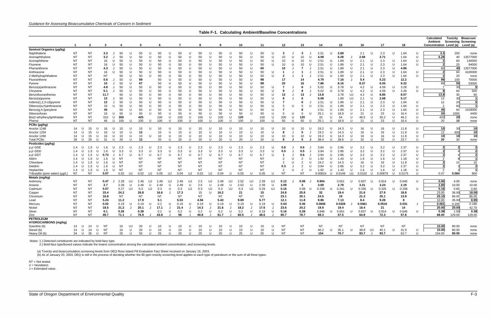
Guidance for Assessing Bioaccumulative Chemicals of Concern in Sediment
State of Oregon Department of Environmental Quality F-3
Table F-1. Calculating Ambient/Baseline Concentrations
Calculated Toxicity Bioaccum Ambient Screening Screening 1 2 3 4 5 6 7 8 9 10 11 12 13 14 15 16 17 18 Concentration Level (a) Level (a)
Semivol Organics (µg/kg)
Naphthalene NT NT 3.3 J 50 U 50 U 50 U 50 U 50 U 50 U 50 U 50 U 3 J 3 J 2.51 U 2.68 2.1 U 2.3 U 1.64 U 3.3 200 none
Acenaphthylene NT NT 3.2 J 50 U 50 U 50 U 50 U 50 U 50 U 50 U 50 U 10 U 10 U 4.08 6.28 J 2.68 3.71 1.64 U 6.28 40 13577000
Acenaphthene NT NT 16 U 50 U 50 U 50 U 50 U 50 U 50 U 50 U 50 U 10 U 10 U 2.51 U 1.89 U 2.1 U 2.3 U 1.64 U 2 60 140000
Fluorene NT NT 16 U 50 U 50 U 50 U 50 U 50 U 50 U 50 U 50 U 10 U 10 U 2.51 U 1.89 U 2.1 U 2.3 U 1.64 U 2 20 94000
Phenanthrene NT NT 4.3 J 50 U 50 U 50 U 50 U 50 U 50 U 50 U 60 10 J 7 J 2.51 U 1.89 U 2.1 U 2.3 U 4.96 60 40 13577000
Anthracene NT NT 16 U 50 U 50 U 50 U 50 U 50 U 50 U 50 U 50 U 1 J 1 J 2.51 U 1.89 U 2.1 U 2.3 U 1.64 U 2 60 4100000
2-Methylnaphthalene NT NT NT 50 U 50 U 50 U 50 U 50 U 50 U 50 U 50 U 2 J 1 J 2.51 U 1.89 U 2.1 U 2.3 U 1.64 U 2 20 none
Fluoranthene NT NT 5.6 J 50 U 69 50 U 50 U 50 U 50 U 50 U 98 17 14 4.79 7.16 J 5.4 5.23 12.2 98 100 70000
Pyrene NT NT 10 J 50 U 67 50 U 50 U 50 U 50 U 50 U 89 20 16 7.86 8.16 8.37 6.05 9.32 89 50 53000
Benzo(a)anthracene NT NT 4.8 J 50 U 50 U 50 U 50 U 50 U 50 U 50 U 50 U 7 J 6 J 5.02 U 3.78 U 4.2 U 4.59 U 3.28 U 7 30 5
Chrysene NT NT 5.1 J 50 U 50 U 50 U 50 U 50 U 50 U 50 U 50 U 9 J 8 J 5.02 U 3.78 U 4.2 U 4.59 U 3.28 U 9 60 500
Benzofluoranthenes NT NT 11.7 50 U 50 U 50 U 50 U 50 U 50 U 50 U 50 U 13 J 13 J 13.8 3.78 UJ 4.2 U 8.85 8.57 13.8 30 50
Benzo(a)pyrene NT NT 13 J 50 U 50 U 50 U 50 U 50 U 50 U 50 U 50 U 8 J 6 5.08 1.89 UJ 2.1 U 2.68 5.17 13 30 1
Indeno(1,2,3-cd)pyrene NT NT 12 J 50 U 50 U 50 U 50 U 50 U 50 U 50 U 50 U 7 6 J 2.51 U 1.89 U 2.1 U 2.3 U 1.64 U 12 20 5
Dibenzo(a,h)anthracene NT NT 16 U 50 U 50 U 50 U 50 U 50 U 50 U 50 U 50 U 5 U 5 U 2.51 U 1.89 U 2.1 U 2.3 U 1.64 U 2 60 1
Benzo(g,h,i)perylene NT NT 45 50 U 50 U 50 U 50 U 50 U 50 U 50 U 50 U 7 8 2.51 U 1.89 U 2.1 U 2.3 U 1.64 U 45 60 1018000
Dibenzofuran NT NT 16 U 50 U 50 U 50 U 50 U 50 U 50 U 50 U 50 U 5 U 5 U 25.1 U 18.9 U 21 U 23 U 16.4 U 20 1000 4400
Bis(2-ethylhexyl)phthalate NT NT 310 U 350 420 100 U 100 U 100 U 100 U 120 100 U 200 U 120 33 U 54 U 48.5 U 30.2 U 46.2 U 420 20 none Phenol NT NT 46 U 100 U 100 U 100 U 100 U 100 U 100 U 100 U 100 U 50 U 50 U 25.1 U 18.9 U 21 U 23 U 16.4 U 20 10 none
PCBs (µg/kg)
Aroclor 1248 14 U 15 U 16 U 10 U 10 U 10 U 10 U 10 U 10 U 10 U 10 U 10 U 10 U 19.2 U 14.3 U 16 U 16 U 11.8 U 10 30 10
Aroclor 1254 14 U 15 U 16 U 10 U 12 10 U 10 U 10 U 10 U 10 U 10 U 8 J 5 J 19.2 U 14.3 U 16 U 16 U 11.8 U 12 600 10
Aroclor 1260 14 U 15 U 16 U 10 U 10 U 10 U 10 U 10 U 10 U 10 U 10 U 10 U 10 U 19.2 U 14.3 U 16 U 16 U 11.8 U 10 10 10 Total PCBs 28 U 29 U 31 U 20 U 12 20 U 20 U 20 U 20 U 20 U 20 U 8 J 5 J 38.4 U 28.6 U 32 U 32 U 23.7 U 20 30 none
Pesticides (µg/kg)
p,p'-DDE 1.4 U 1.5 U 1.6 U 2.3 U 2.3 U 2.3 U 2.3 U 2.3 U 2.3 U 2.3 U 2.3 U 0.8 J 0.6 J 3.84 U 2.86 U 3.2 U 3.2 U 2.37 U 2 2 2
p,p'-DDD 1.4 U 1.5 U 1.6 U 3.3 U 3.3 U 3.3 U 3.3 U 3.3 U 3.3 U 3.3 U 3.3 U 0.5 J 0.5 J 3.84 U 2.86 U 3.2 U 3.2 U 2.37 U 2 4 2
p,p'-DDT 1.4 U 1.5 U 0.73 J 6.7 U 6.7 U 6.7 U 6.7 U 6.7 U 6.7 U 6.7 U 6.7 U 1 J 0.6 J 3.84 U 2.86 U 3.2 U 3.2 U 2.37 U 2 4 2
Aldrin 1.4 U 1.5 U 1.6 U NT NT NT NT NT NT NT NT 2 U 2 U 1.92 U 1.43 U 1.6 U 1.6 U 1.18 U 2 8 1
Chlordane 1.4 U 1.5 U 1.6 U NT NT NT NT NT NT NT NT 2 U 2 U 19.2 U 14.3 U 16 U 16 U 11.8 U 2 10 10
Dieldrin 1.4 U 1.5 U 1.6 U NT NT NT NT NT NT NT NT 0.3 J 2 U 3.84 U 2.86 U 3.2 U 3.2 U 2.37 U 2 3 2
Heptachlor 1.4 U 1.5 U 1.6 U NT NT NT NT NT NT NT NT 2 U 2 U 1.92 U 1.43 U 1.6 U 1.6 U 1.18 U 2 2 1 Tributyltin (pore water) (µg/L) NT NT 0.07 0.02 UJ 0.02 UJ 0.05 UJ 0.04 UJ 0.02 UJ 0.04 U 0.05 U 0.05 U NT NT 0.00816 U 0.0149 UJ 0.0102 U 0.00879 U 0.0175 U 0.07 0.064 800
Metals (mg/kg)
Antimony NT NT 0.47 J 2.28 UJ 2.46 UJ 2.49 UJ 2.49 UJ 2.5 UJ 2.49 UJ 2.52 UJ 2.39 UJ 0.12 J 0.08 J 0.904 0.651 U 0.837 U 0.814 U 0.645 U 0.90 4.00 none
Arsenic NT NT 2.7 2.28 U 2.46 U 2.49 U 2.49 U 2.5 U 2.49 U 2.52 U 2.39 U 3.09 3 3.69 2.78 3.31 3.24 2.19 2.80 10.00 10.00
Cadmium NT NT 0.07 0.27 UJ 0.3 UJ 0.3 U 0.3 UJ 0.3 UJ 0.3 UJ 0.3 UJ 0.29 UJ 0.16 0.08 U 0.339 U 0.261 U 0.335 U 0.325 U 0.258 U 0.16 0.60 0.60
Copper NT NT 15.4 24.2 26.8 16.6 J 17.3 15 U 16.2 21 15 24.8 25.8 32 19.4 21.6 27.9 18.8 23.00 36.00 18.00
Chromium NT NT 16.8 NT NT NT NT NT NT NT NT 23.1 20.1 24.5 19 21.3 25.1 13.9 25.10 86.00 86.00
Lead NT NT 5.24 11.2 17.9 5.1 5.53 4.56 5.43 9.69 5.77 12.1 11.8 9.86 7.13 8.4 9.28 8 10.00 35.00 8.90
Mercury NT NT 0.02 0.19 U 0.19 U 0.2 U 0.19 U 0.19 U 0.19 U 0.19 U 0.19 U 0.04 0.06 0.0606 0.0328 J 0.0461 0.0516 0.031 J 0.061 0.200 0.180
Nickel NT NT 18.5 21.2 J 20.1 J 17.1 J 21.4 J 14.3 J 21.6 J 18.2 J 17.6 J 23.6 20.2 19.9 19.4 18.4 21 14 20.00 20.00 42.70
Silver NT NT 0.1 0.26 0.38 0.2 U 0.2 U 0.2 U 0.2 U 0.2 U 0.19 U 0.16 0.28 0.846 U 0.651 U 0.837 U 0.814 U 0.645 U 0.38 1.00 0.38 Zinc NT NT 49.7 71.1 J 76.9 J 43.8 J 58 J 49.8 J 61.7 J 60.5 J 48.6 J 80.7 78.7 69.3 57.5 64.8 72.3 57.8 68.00 129.00 129.00
PETROLEUM HYDROCARBONS (mg/kg)
Gasoline (b) 14 U 14 U NT 10 UJ 20 U 10 U 10 U 10 U 10 U 10 U 10 U NT NT NT NT NT NT NT 10.00 80.00 none
Diesel (b) 14 U 14 U NT 10 U 20 U 10 U 10 U 10 U 10 U 10 U 10 U NT NT 46.2 U 35.1 U 38.8 UJ 40.1 U 31.9 U 10.00 80.00 none Heavy Oil (b) 34 U 35 U NT 25 U 50 U 25 U 25 U 25 U 25 U 25 U 25 U NT NT 154 70.7 93.7 J 93.7 63.7 U 154.00 80.00 none
Notes: 1.) Detected constituents are indicated by bold-face type.
2.) Bold-face type/boxed values indicate the lowest concentration among the calculated ambient concentration, and screening levels.
(a) Toxicity and bioaccumulation screening levels from DEQ Ross Island Fill Evaluation Fact Sheet received on January 16, 2003. (b) As of January 20, 2003, DEQ is still in the process of deciding whether the 80 ppm toxicity screening level applies to each type of petroleum or the sum of all three types.
NT = Not tested. U = Nondetect. J = Estimated value.

Guidance for Assessing Bioaccumulative Chemicals of Concern in Sediment
State of Oregon Department of Environmental Quality F-4
This page intentionally left blank.

Appendix G.
References

Guidance for Assessing Bioaccumulative Chemicals of Concern in Sediment
State of Oregon Department of Environmental Quality G-1
G. References
ASTM. 1998. Standard Guide for Determination of the Bioaccumulation of Sediment-Associated
Contaminants by Benthic Invertebrates, Standard E-1688-97a. American Society of Testing and
Materials, Philadelphia, PA.
Baudrimont, M., J. Metivaud, R. Maury-Brauchet, F. Ribeyre, and A. Boudou. 1997.
Bioaccumulation and Metallothionen Response in the Asiatic Clam (Corbicula fluminea) After
Experimental Exposure to Cadmium and Inorganic Mercury. Environmental Toxicology and
Chemistry 16:2096-2105.
BCE. 1999. Protocol for Contaminated Sites 4 - Determining Background Soil Quality. British
Columbia Ministry of Water, Land, and Air Protection. Victoria, British Columbia, Canada.
Buck, J. 2004. Environmental Contaminants in Aquatic Resources from the Columbia River,
Study Identifiers: 1130-1F02 and 1261-1N04; On-and Off-Refuge Investigation. US Fish and
Wildlife Service.
Burkhard, L.P. 2000. Factors Influencing The Design Of Bioaccumulation Factor And Biota
Sediment Accumulation Factor Field Studies. Environmental Toxicology and Chemistry 22(2):
351-360.
Burkhard, L.P. 2006. Estimation Of Biota Sediment Accumulation Factor (BSAF) From Paired
Observations Of Chemical Concentrations In Biota And Sediment. U.S. Environmental
Protection Agency, National Health and Environmental Effects Research Laboratory, Duluth,
MN: 29 pp.
Burkhard, L.P., P.M. Cook and D.R. Mount. 2003. The relationship of bioaccumulative
chemicals in water and sediment to residues in fish: A visualization Approach. Environmental
Toxicology and Chemistry 22(11):2822-2830.
California Department of Toxic Substances Control. 2000. Navy/U.S. Environmental Protection
Agency (USEPA) Region 9 Biological Technical Assistance Group (BTAG) Toxicity Reference
Values (TRVs) for Ecological Risk Assessment. Human and Ecological Risk Division. HERD
Ecolgocial Risk Assessment Note Number 4.
DEQ. 2000. Guidance for Conduct of Deterministic Human Health Risk Assessments. Land
Quality Division, Oregon Department of Environmental Quality, Portland, Oregon; May 2000
Update.
DEQ.2001a. Quality Assurance Policy. Land Quality Division, Oregon Department of
Environmental Quality, Portland, Oregon. Final September 1990; Updated April 2001.

Guidance for Assessing Bioaccumulative Chemicals of Concern in Sediment
State of Oregon Department of Environmental Quality G-2
DEQ.2001b. Guidance for Ecological Risk Assessmen. Oregon Department of Environmental
Quality, Final April 1998; Updated December 2001.
Elliot, J.E. and M.L. Harris, 2001/2002. An Ecotoxicological Assessment of Chlorinated
Hydrocarbon Effects on Bald Eagle Populations. Reviews in Toxicology 4:1-60.
Elliot J.E., Norstrom R.J., Lorenzen A., Hart L.E., Philibert H., Kennedy S.W., Stegeman J.J.,
Bellward G.D., and K.M. Cheng, 1996. Biological Effects ofPpoychlorinated dibenzo-p-dioxins,
diobenzofurans, and biphenyls in Bald Eagle (Haliaeetus leucocephalus) Chicks. Environ.
Toxicol. Chem. 15(5):782-793.
Fuhrer, G.J. 1986. Extractable Cadmium, Mercury, Copper, Lead, and Zinc in the Lower
Columbia River Estuary. Oregon and Washington. Water Resources Investigations Report 86-
4088. U.S. Geological Survey, Portland, Oregon.
Fuhrer, G.J. 1989. Quality of Bottom Material and Elutriates in the Lower Willamette River,
Portland Harbor, Oregon. Water Resources Investigations Report 89-4005. U.S. Geological
Survey, Portland, Oregon.
Fuhrer, G.J. and Horowitz, A.J., 1989. The Vertical Distribution of Selected Trace Metals and
Organic Compounds in Bottom Materials of the Proposed Lower Columbia River Export
Channel. Water Resources Investigations Report 95-4294. U.S. Geological Survey, Portland,
Oregon.
Fuhrer, G.J., Tanner, D.O., Morace, J.L., McKenzie, S.W., and Skach, K.A., 1996. Water
Quality of the Lower Columbia River Basin: Analysis of Current and Historical Water-Quality
Data through 1994. U.S. Geological Survey, Portland, Oregon.
Gale, R.W., J.N. Huckins, J.D. Petty, P.H. Peterman, L.L. Williams, D. Morse, T.R. Schwartz,
and D.E. Tillitt, 1997. Comparison Of Uptake Of Dioxin-Like Compounds By Caged Catfish And
Semipermeable Membrane Devices In The Saginaw River, Michigan. Environmental Science and
Technology 31: 178-187.
Henny, C.J., Kaiser, J.L, Grove, R.A., Bentley, V.R., and J.E. Elliott, 2003. Biomagnification
Factors (Fish to Osprey Eggs from Willamette River, Oregon, U.S.A.) for PCDDS, PCBS, and
OC Pesticides. Environmental Monitoring and Assessment, 84: 275-315.
Kubiak, T.J. and D.A. Best., 1991. Wildlife Risks Associated With Passage Of Contaminated,
Anadromous Fish At Federal Energy Regulatory Commission Licensed Dams In Michigan.
Contaminants Program, Division of Ecological Services, East Lansing, Michigan.
Lee, H., III, B.L. Boese, J. Pelliter, M. Winsor, D.T. Specht, and R.C. Randall, 1993. Guidance
Manual: Bedded Sediment Tests. EPA-600/R-93/183, Office of Research and Development, U.S.
Environmental Protection Agency, Washington, DC.

Guidance for Assessing Bioaccumulative Chemicals of Concern in Sediment
State of Oregon Department of Environmental Quality G-3
Mac, M.J., G.E. Noguchi, R.J. Hesselberg, C.C. Edsall, J.A. Shoesmith, and J.D. Bowker, 1990.
A Bioaccumulation Bioassay for Freshwater Sediments. Environmental Toxicology and
Chemistry 9: 1405-1414.
MacCoy, D.E. and Black, R.W., 1998. Organic Compounds and Trace Elements in Freshwater
Streambed Sediment and Fish from the Puget Sound Basin. USGS Fact Sheet 105-98. Puget
Sound Basin NAWQA Study, U.S. Geological Survey, Seattle, Washington.
Meador, J.P., Clark Jr., R.C., Robisch, P.A., Ernest, D.W., Landahl, J.T., Varanasi, U., Chan, S-
L., and McCain, B.B., 1994, National Benthic Surveillance Project: Pacific Coast. Analyses of
Elements in Sediment and Tissue Cycles I to V (1984-88). NOAA Technical Memorandum
NMFS-NWFSC-16, National Marine Fisheries Service, National Oceanic and Atmospheric
Administration, Seattle, Washington
Nagpal, N. K. and Howell, K., 2001. Water Quality Guidelines for Selenium, Technical
Appendix. British Columbia Ministry of Water, Land, and Air Protection, Victoria, British
Columbia, Canada.
Nozaki, Y., 1997, A Fresh Look at Element Distribution in The North Pacific. EOS electronic
supplement, posted May 27, 1997. [www.agu.org/eos_elec/]
Millsap, S.D. et al., 2004. Comparison of Risk Assessment Methodologies for Exposure of Mink
to PCBs on the Kalamazoo River, Michigan. Environmental Science & Technology.
38(24):6451-6459.
Posthuma, L., G.W. Sutter and T.P. Trias, 2001. Species Sensitivity Distributions in
Ecotoxicology. CRR Press, Boca Raton, Florida, U.S.A.
Quinby-Hunt, M.S. and Turekian, K.K., 1983. Distribution of Elements in Sea Water. EOS, 64:
130-131.
Quinby-Hunt, M.S. and Wilde, P., 1986/87. Modeling of Dissolved Elements in Sea Water.
Ocean Science and Engineering, 11:3,4:153-251.
Rice, C.P. and D.S. White, 1987. PCB Availability Assessment of River Dredging Using Caged
Clams and Fish. Environmental Toxicology and Chemistry 6: 4:259-274.
Rickert, D.A., Kennedy, V.C., McKenzie, S.W., and Hines, W.G., 1977. A Synoptic Survey of
Trace Metals in Bottom Sediments of the Willamette River, Orego. Geological Survey Circular
715-F. U.S. Geological Survey, Arlington, Virginia.
Sample, B.E., D.M. Opresko, and G.W. Suter II, 1996. Toxicological Benchmarks for Wildlife.
ES/ER/TM-86/R3. Oak Ridge National Laboratory, Oak Ridge, TN.

Guidance for Assessing Bioaccumulative Chemicals of Concern in Sediment
State of Oregon Department of Environmental Quality G-4
Shephard, B.K. 1998. Quantification of Ecological Risks for Aquatic Biota from Bioaccumulated
Chemicals. In National Sediment Bioaccumulation Conference Proceedings, U.S.
Environmental Protection Agency, Office of Water, Washington D.C. EPA 823-R-98-0023: pp
2-31 – 2-52.
Steevens, J.A., Reiss, M.R. and A.V. Pawlisz. 2005. A Methodology for Deriving Tissue
Residue Bbenchmarks for Aquatic Biota: A Case Study for Fish Exposed to 2,3,7,8-
Tetrachlorodibenzo-p-dioxin and Equivalents. Integrated Environmental Management, 1(2):142-
151.
Tillitt D.E., Gale R.W., Meadows J.C., Zajicek J.L., Peterman P.H., Heaton S.N., Jones P.D.,
Bursian S.J., Kubiak T.J., Giesy J.P., Aulerich R.J., 1996. Dietary Exposure of Mink to Carp
from Saginaw Bay 3. Characterization of Ddietary Exposure to Planar Halogenated
Hydrocarbons, Dioxin Equivalents, and Biomagnification. Environmental Science &
Technology 30:283-291.
USEPA, 1989. Risk Assessment Guidance for Superfund: Volume I - Human Health Evaluation
Manual (Part A), Interim Final. EPA/540/1-89/002, Office of Emergency and Remedial
Response, U.S. Environmental Protection Agency.
USEPA, 1995. Great Lakes Water Quality Initiative Criteria Documents for the Protection of
Wildlife, DDT, Mercury, 2,3,7,8-TCDD, PCBs. U.S. Environmental Protection Agency, Office of
Water, Washington, D.C. EPA-820-B-95-008.
USEPA, 1996. Soil Screening Guidance: Technical Background Document. U.S. Environmental
Protection Agency, Office of Solid Waste and Emergency Response, EPA/540/R-95/128.
USEPA, 1997. Guidance for Assessing Chemical Contamination Data for Use in Fish
Advisories, Volume 2, Risk Assessment and Fish Consumption Limits. Second Edition, EPA 823-
B-97-009. Office of Water, U.S. Environmental Protection Agency, Washington DC.
USEPA, 2000. Methods for Measuring the Toxicity and Bioaccumulation of Sediment-associated
Contaminants with Freshwater Invertebrates. Second Edition, EPA 600/R-99/064. Office of
Research and Development, U.S. Environmental Protection Agency, Duluth, MN.
USEPA, 2002a. Role of Background in the CERCLA Cleanup Program. OSWER 9285.6-07P.
U.S. Environmental Protection Agency, Office of Solid Waste and Emergency Response,
Washington DC.
USEPA, 2002b. Guidance for Comparing Background and Chemical Concentrations in Soil for
CERCLA Sites, Appendix B: Policy Considerations for the Application of Background Data in
Risk Assessment and Remedy Selection. EPA 540/R-01/003, OSWER 9285.7-41. U.S.

Guidance for Assessing Bioaccumulative Chemicals of Concern in Sediment
State of Oregon Department of Environmental Quality G-5
Environmental Protection Agency, Office of Solid Waste and Emergency Response, Washington
DC.
USEPA, 2002c. Columbia River Basin Fish Contaminant Survey, 1996-1998. EPA 910/R-02-
006. U.S. EPA, Region 10, Seattle, WA.
USEPA. 2003. Analyses of Laboratory and Field Studies of Reproductive Toxicity in Birds
Exposed to Dioxin-like Compounds for use in Ecological Risk Assessment. EPA/600/R-03/114F.
USEPA. 2004. National Recommended Water Quality Criteria. Office of Water, Office of
Science and Technology, EPA 4304T.
USEPA. 2006. Ecological Soil Screening Levels. Interim Eco-SSLs and Documentation.
[http://www.epa.gov/ecotox/ecossl/index.html]
USEPA/USACE. 1991. Evaluation of Dredged Material for Ocean Disposal - Testing Manual
(Draft), EPA 503/8-91/001, Office of Water. U.S. Environmental Protection Agency and U.S.
Army Corps of Engineers, Washington, DC.
USEPA/USACE. 1994. Evaluation of Dredged Material Proposed for Discharge in Waters of
the U.S. - Testing Manual (Inland Testing Manual). EPA-823-B-94-002, Office of Water, U.S.
Environmental Protection Agency and U.S. Army Corps of Engineers, Washington, DC.
USEPA/USACE. 2006. Northwest Regional Sediment Evaluation Framework. Interim Final.
U.S. Army Corps of Engineers,
http://www.nws.usace.army.mil/publicmenu/DOCUMENTS/DMMO/RSET_Interim_Final.pdf
Van den Berg, M. et. al. 1998. Toxic Equivalency Factors (TEFs) for PCBs, PCDDs, PCDFs for
Humans and Wildlife. Environmental Health Perspectives. 106(12): 775-792.
Van den Berg, M. et al. 2006. The 2005 World Health Organization Re-evaluation of Human
and Mammalian Toxic Equivalency Factors for Dioxins and Dioxin-like Compounds. ToxSci
advance access copy published 7 July, 2006.
WDOE. 1994. Natural Background Soil Metal Concentrations in Washington State. Publication
#94-115. Washington Department of Ecology, Olympia, WA.
WDOE. 1998. Analyzing Site or Background Data With Below-Detection Limit or Below-PQL
Values (Censored Data). Supplement S-6 to Statistical Guidance for Ecology Site Managers,
Washington Department of Ecology.
WDOH. 1995. Development of Sediment Quality Criteria for the Protection of Human Health.
Tier I Report. Office of Toxic Substances, Washington Department of Health.

Guidance for Assessing Bioaccumulative Chemicals of Concern in Sediment
State of Oregon Department of Environmental Quality G-6
Wiemeyer, S.N., T.G. Lamont, C.M. Bunck, C.R. Sindelar, F.J. Gramlich, J.D Fraser, M.A.
Byrd. 1984. Organochlorine pesticide, polychlorobiphenyl, and mercury residues in bald eagle
eggs - 1969 -79-and their relationships to shell thinning and reproduction. Archives of
Environmental Contamination and Toxicology.13:529-549.
Wiemeyer, S.N., C.M. Bunck, A.J. Krynitsky. 1988. Organochlorine pesticides, polychlorinated
biphenyls, and mercury in osprey eggs - 1970-79- and their relationships to shell thinning and
productivity. Archives of Environmental Contamination and Toxicology. 17:767-787.
Wiemeyer, S.N., C.M Bunck, C.J. Stafford. 1993. Environmental Contaminants in Bald Eagle
Eggs - 1980-84- and Further Interpretations of Relationships to Productivity and Shell
Thickness. Archives of Environmental Contamination and Toxicology, 24:213-227.