pure.tue.nl thesis (1cm96) david brandstÄdter, bsc student identity number 0785856 . in partial...
TRANSCRIPT

Eindhoven University of Technology
MASTER
The impact of prices and maintenance activities on business cycles in the upstreamprocess industry
Brandstädter, D.
Award date:2013
DisclaimerThis document contains a student thesis (bachelor's or master's), as authored by a student at Eindhoven University of Technology. Studenttheses are made available in the TU/e repository upon obtaining the required degree. The grade received is not published on the documentas presented in the repository. The required complexity or quality of research of student theses may vary by program, and the requiredminimum study period may vary in duration.
General rightsCopyright and moral rights for the publications made accessible in the public portal are retained by the authors and/or other copyright ownersand it is a condition of accessing publications that users recognise and abide by the legal requirements associated with these rights.
• Users may download and print one copy of any publication from the public portal for the purpose of private study or research. • You may not further distribute the material or use it for any profit-making activity or commercial gain
Take down policyIf you believe that this document breaches copyright please contact us providing details, and we will remove access to the work immediatelyand investigate your claim.
Download date: 18. May. 2018
MASTER THESIS (1CM96)
DAVID BRANDSTÄDTER, BSC STUDENT IDENTITY NUMBER 0785856
IN PARTIAL FULFILMENT OF THE REQUIREMENTS FOR THE DEGREE OF
MASTER OF SCIENCE
IN OPERATIONS MANAGEMENT AND LOGISTICS
SUPERVISED BY:
PROF. DR. J. C. FRANSOO, TU/E DR. B. WALRAVE, TU/E
BEN DE WEERD, BSC, SABIC PAUL STEIJNS, MA MSC, SABIC
OPERATIONS MANAGEMENT AND LOGISTICS EINDHOVEN UNIVERSITY OF TECHNOLOGY
EINDHOVEN, 1ST OF JULY 2013
THE IMPACT OF PRICES AND MAINTENANCE ACTIVITIES ON BUSINESS CYCLES IN THE
UPSTREAM PROCESS INDUSTRY
BY
DAVID BRANDSTÄDTER

The Impact of Prices and Maintenance Activities on Business Cycles in the Upstream Process Industry 2
David Brandstädter | [email protected] Jul 2013
TUE SCHOOL OF INDUSTRIAL ENGINEERING.
SERIES MASTER THESES OPERATIONS MANAGEMENT AND LOGISTICS
SUBJECT HEADINGS: SUPPLY CHAIN DYNAMICS, BUSINESS CYCLE FORECASTING, SYSTEM DYNAMICS, COMMODITY INDUSTRY, PRICE FORECASTING

I Abstract
Master Thesis TU/e Eindhoven
ABSTRACT
We show that large-scale maintenance activities typical to the upstream process industry explain a fair share of product price spread variance of commodity chemicals. A forecast model covering a six months horizon for relevant product price spreads based on planned maintenance activities, historical oil prices and GDP growth is created.
A proven System Dynamics model is applied to a hydrocarbon supply chain providing a volume forecast feature. The model builds further evidence on the Lehman Wave destocking effect observed in supply chains. Based on findings of an extensive calibration analysis, recommendations for further applications of the model are given.

The Impact of Prices and Maintenance Activities on Business Cycles in the Upstream Process Industry II
David Brandstädter | [email protected] Jul 2013
EXECUTIVE SUMMARY
This study investigates structural and dynamic reasons for high fluctuation in price and demand observed in the upstream plastics supply chain in Europe. The work covers a time span of eight years (2005 to 2012) covering the disrupting and severe effect of the financial crisis triggered by the Lehman bankruptcy in September 2008 and leading to a recessive phase with long-lasting weak demand in Europe. Supply chains have been exposed to a synchronised destocking effect coined the “Lehman Wave”. Figure 1 depicts the elements in scope. The polymers discussed are HDPE, LDPE and LLDPE. All data used is aggregated to a European industry level.
close integration
4Cracker
Units
3Polymer
Units
2 Converters
1OEMs
Consumer End
Markets
Genericfeedstock
Ethylene Poly-ethylene
Plasticproduct
Finalproduct
FIGURE 1: SUPPLY CHAIN OF PLASTICS IN SCOPE
Two models have been developed to address the problem: a) a price spread forecast model based on multiple linear regression analysis and b) a System Dynamics supply chain model including a forecast feature for ethylene production and polyethylene inventory levels (see Figure 2).
Maintenance-Price Model Supply Chain Model
6 months forecast horizon PE- and C2/Naphtha spread Based on crude oil price, planned
maintenance and GDP growth Explains up to 69% of variance Multiple Linear Regression
2007 - 2012 horizon + forecast Production, stock and order of all
four echelons Based on end-market demand .814 R²-fit of descriptive part System Dynamics
FIGURE 2: KEY MODEL FEATURES
Context
Since the Lehman Shock, European demand for ethylene has been weak. As there has been hardly any capacity adjustment, utilisation rates remain significantly below those of the prior crisis state. At the same time, prices showed increased volatility, in particular those for HDPE.
Large-scale maintenance activities are a characteristic of the petrochemical industry. Cracker units, which convert feedstock such as naphtha to ethylene and other by-products, need to undergo full maintenance approximately every six years. Such “turnarounds” last for about forty days forcing producers to careful planning of operations and material sourcing from competitors. This is necessary because inventory capacity is not sufficient to buffer over the entire period. Due to weather conditions and contractor availability, turnarounds are highly seasonal. Maintenance schedules are known up to one year in advance and the industry is experienced in dealing with the dynamics imposed through a “turnaround season”.

III Executive Summary
Master Thesis TU/e Eindhoven
Maintenance-Price Model
Since 2009, the extent of planned maintenance activities such as cracker-turnarounds has an effect on commodity prices detectable in spreads. The extent of maintenance explains around 25% of the observed variance in ethylene-naphtha and polyethylene-naphtha spreads. Due to low deviation from the published schedules, the quantified effect is suitable for forecasting. Figure 3 shows the 𝑅²-values for a regression model utilising the planned maintenance extent, crude oil price (respectively its lags) and GDP growth.
FIGURE 3: EXPLANATORY POWER OF THE REGRESSION MODEL
Supply Chain Model
Studies conducted in the industry showed that the distinct drop in production, known as Lehman Wave, was caused by synchronised de-stocking throughout the value chain (Udenio, et al., 2012). A System Dynamics model previously applied to the industry (Corbijn, 2013) is extended to the ethylene producer echelon and end markets characterised by application (e.g. food, construction) rather than production technique (e.g. blow moulding). The model is calibrated against data of industry reports but eventually solely reacts on end-market demand, the only input. Outputs of the model show an 𝑅²-value of .814 for the ethylene production from 2007-2012 (see Figure 4). The forecast feature of the model is able to capture upcoming ramp-ups and overshoots but requires interpretation and is prone to miss inter-month shifts due to the interpolation of monthly input data.
FIGURE 4: SUPPLY CHAIN MODEL FIT
.595
.688
.676
.611
.538 .493 .481
.616
.693
.671 .611 .551
.512 .501
.000
.100
.200
.300
.400
.500
.600
.700
.800
.900
1.000
0 -1 -2 -3 -4 -5 -6
R² (Naphtha spread)
Crude Oil Price Lag
Regression model R²s (predictors: planned, crude oil price, GDP)
Ethylene
HDPE
-
20
40
60
80
100
120
140
Jan 07 Jun 07 Nov 07 Apr 08 Sep 08 Feb 09 Jun 09 Nov 09 Apr 10 Sep 10 Feb 11 Jul 11 Nov 11 Apr 12 Sep 12
[Units/Week] Ethylene Production Levels
Modelled Observed
The Impact of Prices and Maintenance Activities on Business Cycles in the Upstream Process Industry IV
David Brandstädter | [email protected] Jul 2013
This means a model only reacting on end-market demand rather than that of direct customers can explain a great deal of upstream production flows. Confirming the Bullwhip Effect, the model reacts most sensitive to changes in the end-market amplifying demand shifts throughout the chain leading to severe oscillation at the upstream echelon. The model further shows high sensitivity to changes in desired inventory coverage of Echelon 4 (ethylene production) and Echelon 3 (polyethylene production).
When price is introduced to the model, order size reacts on movements in price. This effect grows in absolute terms in the second half of the observed period (post-Lehman) compared to the first half (pre-Lehman). Further it could be shown that calibrating the model only in the post-Lehman period leads to a significantly worse model fit. This indicates that the post-Lehman period shows strong instability. Once the model is calibrated from a pre-Lehman point of view the fit increases considerably indicating that the model needs its memory to correctly react on disturbance. From a modelling point of view this means that any System Dynamics approach to explain the industry’s supply chain has to be calibrated from a relatively stable and balanced environment. From a managerial point of view this means that any planning decision should take into account past measures and responses which may not yet have been absorbed by the system.
Despite the strong effect of planned maintenance activity on price spreads, adding capacity limitations to the supply chain model does not add significant value in terms of model fit. This indicates that production volume on a market level is not influenced by cracker outages. Further, imports of polyethylene to the European market also do not influence production levels whereas they have an effect on prices.
Merged finding from both models
Both models have in common that the Lehman Shock marked the beginning of a new period characterised by instability and nervousness. Only since 2009 price spreads react on large-scale maintenance activities. Likewise, the effect of price on order size has increased. On the other hand, a model only taken into account volumes and excluding price can explain a great deal of the variance in ethylene production and polyethylene stock levels. This leads to the conclusion that price alone cannot be a proxy for demand but has to be seen in combination with volume.

V Preface
Master Thesis TU/e Eindhoven
PREFACE
This thesis project has been designed, developed and executed over the course of one and a half years. Whereas many people were more than willing to help, a few stand out. I would like to thank
Hilde & Detlef Brandstädter,
Maria-Alexandra Bujor,
Jan Fransoo,
Paul Steijns,
Maxi Udenio,
Bob Walrave,
Ben de Weerd.
Without their strong support, this endeavour would simply not have been possible.
The Impact of Prices and Maintenance Activities on Business Cycles in the Upstream Process Industry VI
David Brandstädter | [email protected] Jul 2013
TABLE OF CONTENTS
Abstract ................................................................................................................................................................................... I
Executive Summary ......................................................................................................................................................... II
Preface ................................................................................................................................................................................... V
Table of Contents ............................................................................................................................................................. VI
1 Introduction to the Petrochemical Industry ....................................................................................................... 1
1.1 The Petrochemical Industry .............................................................................................................................. 1
1.1.1 Situation in Europe ....................................................................................................................................... 2
1.1.2 Recent Developments .................................................................................................................................. 3
1.2 SABIC ........................................................................................................................................................................... 4
1.3 Cracker ....................................................................................................................................................................... 4
1.3.1 Invest and Position in the Supply Chain .............................................................................................. 4
1.3.2 European Cracker Fleet .............................................................................................................................. 5
1.3.3 Cracker Maintenance ................................................................................................................................... 6
1.4 Prices and Contracting ......................................................................................................................................... 8
1.4.1 Contract and Spot Sales .............................................................................................................................. 8
1.4.2 Increased Price Volatility ........................................................................................................................... 9
1.5 The Supply Chain of Plastics .......................................................................................................................... 10
1.5.1 Players in the Value Chain ...................................................................................................................... 10
1.5.2 Transport and Inventory ......................................................................................................................... 11
1.5.3 Global Market ............................................................................................................................................... 11
1.6 Project Layout ...................................................................................................................................................... 12
1.6.1 Project Scope ................................................................................................................................................ 12
1.6.2 Project Approach ........................................................................................................................................ 13
2 Literature Review........................................................................................................................................................ 14
2.1 Supply Chain Dynamics .................................................................................................................................... 14
2.2 Commodity Pricing and Volatility ................................................................................................................ 15
2.3 Identified Gaps ..................................................................................................................................................... 16
3 Research Contribution .............................................................................................................................................. 17
3.1 Problem Statement ............................................................................................................................................ 17
3.2 Research Questions ............................................................................................................................................ 17
3.3 Research Methodology ..................................................................................................................................... 18
4 Maintenance-Price Model ........................................................................................................................................ 21
4.1 Effect on Price Spreads ..................................................................................................................................... 22
4.1.1 Correlation Analysis .................................................................................................................................. 22
VII Table of Contents
Master Thesis TU/e Eindhoven
4.1.2 Regression Analysis ................................................................................................................................... 23
4.1.3 Extended Regression Analysis .............................................................................................................. 26
4.2 The Effect on Converter Order Behaviour ................................................................................................ 28
4.2.1 Order Behaviour in Times of High Price Volatility ....................................................................... 29
4.2.2 Order Behaviour in Times of Low Price Volatility ........................................................................ 29
4.3 Model Results ....................................................................................................................................................... 29
4.3.1 Influence of Market Capacity ................................................................................................................. 30
4.3.2 Forecast Ability ........................................................................................................................................... 30
5 Basic Supply Chain model ........................................................................................................................................ 31
5.1 Baseline Version .................................................................................................................................................. 33
5.1.1 Parameter Estimation .............................................................................................................................. 37
5.1.2 Model Verification ...................................................................................................................................... 39
5.1.3 Model Validation ......................................................................................................................................... 40
5.1.4 Model Results ............................................................................................................................................... 43
5.1.5 Forecast .......................................................................................................................................................... 44
5.2 Extension: Capacity Shortage ........................................................................................................................ 46
5.3 Extension: Imports ............................................................................................................................................. 47
6 Advanced Supply Chain Model .............................................................................................................................. 48
6.1 Parameter Estimation ....................................................................................................................................... 48
6.2 Model Fit/Added Value .................................................................................................................................... 51
7 Managerial Insights .................................................................................................................................................... 52
7.1 General Insights ................................................................................................................................................... 52
7.2 Insights and Application of the Maintenance-Price Model ................................................................ 52
7.3 Insights and Application of the Supply Chain Model............................................................................ 53
8 Conclusion and Further Research ........................................................................................................................ 55
8.1 Conclusion ............................................................................................................................................................. 55
8.1.1 Hypotheses .................................................................................................................................................... 55
8.1.2 Research Questions ................................................................................................................................... 56
8.1.3 Limitations .................................................................................................................................................... 58
8.2 Further Research ................................................................................................................................................ 58
9 List of Abbreviations ...................................................................................................................................................... i
10 List of Figures ................................................................................................................................................................ ii
11 List of Tables ................................................................................................................................................................ iii
12 Appendices .................................................................................................................................................................... iv
Appendix A Supplementary Figures ...................................................................................................................... v
Appendix B Background Information .................................................................................................................. ix
The Impact of Prices and Maintenance Activities on Business Cycles in the Upstream Process Industry VIII
David Brandstädter | [email protected] Jul 2013
Appendix C Regression Results and Tests ......................................................................................................... xi
Appendix D Supply Chain Model Tests ............................................................................................................. xvi
Appendix E Model M1A Capacity Limitation Analysis ............................................................................... xxi
Appendix F Supply Chain Model Parameters .............................................................................................. xxiii
Appendix G Model M1B Forecast for Early Horizon ................................................................................ xxxii
Appendix H Upstream/Downstream Interface ........................................................................................ xxxiii
13 References ............................................................................................................................................................... xxxv

1 Introduction to the Petrochemical Industry
Master Thesis TU/e Eindhoven
1 INTRODUCTION TO THE PETROCHEMICAL INDUSTRY
The petrochemical industry is an industry of throughput-focused production techniques and multifaceted market dynamics. This introductory chapter is aiming at giving a comprehensive overview of aspects relevant for the conducted study followed by a note on the project’s scope and layout.
An overview of the current literature in supply chain dynamics, commodity pricing and the chosen modelling technique, System Dynamics, is given in Chapter 2. Chapter 3 outlines the contribution to current research, explains the methodology of the study. Chapter 4, 5 and 6 discuss the statistical and the supply chain models as well as extracted findings. In Chapter 7, managerial insights are presented. Chapter 8 concludes the work and provides outlook to further research. Detailed statistical results and background information supplementing the line of thought demonstrated in the main chapters can be found in the appendix. A reference to a figure or table which includes a letter refers to the appendix.
1.1 THE PETROCHEMICAL INDUSTRY
Considering that the first commercial oil well in the United States was drilled in 1859 by Edwin Drake in Titusville, Pennsylvania (American Manufacturer and Iron World, 1901), the petrochemical industry is relatively young as it only gained importance in the World War II years around 1940. The demand for synthetic materials increased, mostly to replace costly “natural” products. The industrial focus was quickly broadened and expanded to goods like kitchen appliances, textiles, nylons, all sorts of plastics, medical devices, fertilisers, packaging and many more (APPE, 2006). Providing an exhaustive list of end products and applications for this industry can be claimed to be impossible and easily exceeds thousands of items.
FIGURE 5: FEEDSTOCK AND MAIN PRODUCTS OF A CRACKER – ADAPTED FROM BEYCHOK (2012)
The industry is highly divergent as only two major import streams (naphtha and gas feeds) from petroleum refineries or natural gas processing build the first step of the production chain. Figure 5 illustrates this first processing step in the petrochemical industry. Naphtha is a liquid by-product in the oil refinery process; Ethane, propane, butane and methane are gaseous by-products of gas production. Cracker production units are dedicated to a certain type of feedstock

The Impact of Prices and Maintenance Activities on Business Cycles in the Upstream Process Industry 2
David Brandstädter | [email protected] Jul 2013
but allow flexibility to some extent. The created products ethylene and propylene are categorised as olefins. C4 derivatives (e.g. butadiene) build a group on their own, benzene and higher by-products are called aromatics1. “Higher” refers to the number of carbon atoms per molecule. Products with more carbon atoms are also referred to as “heavier” products. Figure A-1 shows an extended view of the cracker derivatives. Usually the transport of the cracker feeds marks the end of the oil industry and the beginning of the petrochemical industry. The distinction between petrochemical and chemical industry is, however, less clear and can only be described by a continuum.
Ethylene and propylene comprise the largest volume of the petrochemical material stream and are used as monomer and chemical feedstock. Due to its capital intensity and for historic reasons the petrochemical industry is dominated by large players, some of which belong to the biggest companies in the world. The worldwide chemical industry has been growing steadily for decades and its growth is usually slightly above the growth rate of the GDP. Strongly growing markets for both production and sales are Asia, in particular China, as well as Latin America. The NAFTA region and the EU are still net exporters of chemicals in trade terms with the EU accounting for nearly 40% of global trade value (see Figure 6).
FIGURE 6: WORLDWIDE IMPORT AND EXPORT OF CHEMICALS IN VALUE (CEFIC, 2012)
The worldwide chemical market is estimated to be 2 744 billion euro in 2011. The EU market share for 2011 was 20% (539 bln €) – a major decline from former 36% (295 bln €) in 1991.
1.1.1 SITUATION IN EUROPE
The chemical industry is a European key industry with an average yearly growth in total export of 6.9% among EU member states in the period of 2000 to 2011. The industry is of major concern for the Netherlands’ economy. The Dutch chemical and process industry market is consolidated and mature. A handful of major actors compete for customers and raw material. Recently, a project was initiated within the industry to investigate benefits of increased horizontal collaboration between formal competitors in order to achieve mutual benefits in terms of cost, efficiency and environmental footprints (DINALOG, 2012).
The financial and the following European economic crisis had and still have strong impact on the industry. The “Lehman Wave” (Peels, et al., 2009) showed that the industry is prone to
1 The name aromatics stems from their “distinctive perfumed smell” (APPE, 2006).
43%
34%
14% 5%
2% 2%
World export of chemicals (2011)
EU Asia NAFTA Rest of Europe Latin America Africa & Oceania
37%
37%
11% 6%
6% 3%
World import of chemicals (2011)

3 Introduction to the Petrochemical Industry
Master Thesis TU/e Eindhoven
destocking effects of the supply chain and unveiled significant overcapacity of production units. European units have no feedstock price advantage over other production regions and are particularly sensitive to naphtha and other feedstock prices. Rationalising production capacity and closing cracker units has hardly taken place since the shock of the “Lehman Wave”. Cracker units are a large-scale investment and have long amortisation times (see 1.3.1). Often they are connected to a chemical cluster or an integrated complex - workplaces for thousands of employees. Closing or mothballing a unit has strong social and financial effects for a region and thus operations are partly subsidised by local governments. The spread between available capacity2 and actual production has widened since the Lehman Shock. Whereas the capacity of end 2012 is almost identical to that of early 2005, the production has dropped by around 20%. In comparison, the EU-27 GDP as of end 2012 is on an inflation corrected level of 6.8 % above those of early 2005 (Eurostat, 2013).
Although the net production capacity has hardly changed, the European petrochemical industry did undergo structural changes since the Lehman Shock. Certain players divested polymer units or temporary closed cracker facilities: Dow sold its four polypropylene plants to Brazilian Breskem (Dow, 2011) and its polystyrene unit “Styron” to Bain Capital (Reuters, 2010). Shell shut down its Wesseling 2B cracker in Germany (Andy Gibbins, 2010) – to only name a few developments.
1.1.2 RECENT DEVELOPMENTS
The topic which is discussed the most in recent years and often acclaimed to be the “next big thing” (The Economist, 2012) in the industry is the use of shale gas and the related hydraulic fracturing technology, better known as “fracking” (Getches-Wilkinson Center, 2013). The United States have established shale gas exploitation on a large scale and have increased the amount of accessible gas reservoirs considerably. The country is expected to be independent of energy fuel imports by 2030 and become one of the biggest gas and oil producers (CNN Money, 2012). Natural gas prices have dropped considerably already, giving the US a “feedstock price advantage” – a cheaper access to feedstock than competitors. Ethane and other derivatives of natural gas can be used as cracker input (see Figure 5). Considerable investment in cracking capacity has already taken place in the United States or is expected. Compared to 2012, ethane cracking capacity could rise by 40% in 2018 (Financial Times, 2012). Consequently derivative production capacity is increased in a similar magnitude, lowering the country’s dependency on imports. Gas cracking compared to naphtha cracking has the disadvantage that no butadiene and other heavier by-products are produced. This led to a butadiene rally causing price spikes even in Europe.
The cheap access of the US to feedstock also sets the Middle East region under pressure which in the past had access to the cheapest feedstock worldwide in the magnitude of 50% of that of the European price. This new development could lead to a focus on efficiency and possible investments because cost price is not a unique position anymore.
Next to feedstock availability from a supply side, lightweight and multi-layer technologies are driving factors for the demand side of the plastic industry (ResearchAndMarkets, 2013).
2 The available capacity is the nameplate (or nominal) capacity minus the loss due to maintenance activities or (temporary) plant closures. According to the PMRC report published by the APPE (Association of Petrochemicals Producers in Europe, 2011), the nominal capacity is the “maximum yearly production capacity which is available in the public domain”.

The Impact of Prices and Maintenance Activities on Business Cycles in the Upstream Process Industry 4
David Brandstädter | [email protected] Jul 2013
1.2 SABIC
SABIC, the Saudi Basic Industries Corporation, is one of the largest non-oil chemical companies with its headquarter and origin in Riyadh, Saudi Arabia. The company is listed at Tadawul, Saudi Stock Exchange, with the Saudi Arabian state owning around 70% of its shares. It was founded in 1976 by royal decree. In 2002, SABIC started production activity in Europe by acquiring DSM and obtaining production capacity in Sittard-Geleen, the Netherlands, as well as in Gelsenkirchen, Germany. European business was further extended in 2007 when SABIC took over plants of the Huntsman Corporation in the UK.
In 2011, the company owned assets of ca. 67 bln € and achieved a revenue of 39 bln € yielding a net income of 5.8 bln € (SABIC, 2012). 69 million metric tons of products were produced. SABIC operates production units in more than 40 countries and has an employee count of around 30 000 (SABIC, 2013). SABIC is organised in six strategic business units (SBUs): Chemicals, Performance Chemicals, Polymers, Innovative Plastics, Fertilizers and Metals.
1.3 CRACKER
Naphtha crackers (also steam crackers) are some of the most complex and technologically advanced processing units in petrochemistry and build, after crude oil refining, often the head of a chemical supply chain. Naphtha crackers split up (“crack”) longer-chain liquid hydrocarbons such as naphtha (petroleum) and gas oil or gases like propane and ethane and convert them into short-chain hydrocarbons such as ethylene, propylene (propene), C4-fractions, pygas, aromatics, hydrogen and methane. The composition of the achieved output depends mainly on the input material. “Heavy”, longer-chained naphtha creates a higher proportion of longer-chained outputs.
1.3.1 INVEST AND POSITION IN THE SUPPLY CHAIN
Building a naphtha cracker is extremely expensive and even leading chemical companies in Europe only own a few crackers (see Table B-2). In order to compensate for the high upfront investment, naphtha crackers are usually operated on very high utilisation levels. The largest naphtha cracker in the world is located in Port Arthur, Texas and is co-owned by BASF and Total Petrochemicals. It has a capacity of 920 metric kilotons of ethylene per year (Total Petrochemicals USA, Inc., n.d.). For this output, roughly three times the amount of naphtha is needed (Wikipedia, 2012).
The profitability of a cracker asset depends on several main factors. Technology determines the efficiency of resource input versus achieved output. Age often coincides with technology level but in addition partly determines the extent and frequency of maintenance activities. Size and scale are additional factors defining margin profitability. The average asset scale has more than doubled compared to the 1970s. Location is a key factor because it determines access to feedstock and the quoted feedstock prices. Related to location is the level of integration with subsequent but also feedstock units.
Successive processes are often directly linked to the naphtha cracker output stream and production is often dedicated to captive demand. An unforeseen shutdown has severe consequences for these tied processes which is another reason for the thorough maintenance of a cracker unit. However, due to the high utilisation and the low number of crackers, a shutdown for maintenance takes considerable capacity out of the regional market which needs to be buffered by (increased) safety stocks and constrained purchases from competitors. An additional challenge is to control the in- and outflows of cracker and subsequent units. The nature of chemical production sets high requirements to feasible throughput values – starving is

5 Introduction to the Petrochemical Industry
Master Thesis TU/e Eindhoven
as much a critical issue as is storage limitation. A chemical tank has a hard fill rate limit and is often dedicated to a certain subset of products.
1.3.2 EUROPEAN CRACKER FLEET
European cracker capacity has remained nearly constant over the last decade. No new plants have been built since the 1990s and aside of major refurbishment processes, capacity only increased due to efficiency gains. Figure A-2 shows the location of the around 45 crackers in Europe many of which are grouped on a single cluster location (e.g. Antwerp, Carling, Geleen, Grangemouth, Tarragona, Terneuzen etc.). The map can be divided in five segments: South (consisting of Portugal, Spain, Southern France and Italy including Sardinia), Central (North of France, Belgium, the Netherlands and Western Germany), North (Norway, Sweden, and Finland), East (Eastern Germany and Austria) and UK (isolated as an island with no continental pipeline connection). Figure 7 compares the capacity of the defined clusters and underlines the pre-eminence of the Central cluster: In 2012, 58% of all European cracker capacity was concentrated here.
The European cracker fleet is mainly one of liquid (heavy) naphtha feeds. In the long run, this could lead to a competitive advantage over the US and Middle East region as their (new) cracker installations are mainly gas and light feed units which are unable to produce higher olefins. An additional characteristic of the European fleet is the considerable high age of its production units. Thorough, frequent maintenance and overhauling activities ensure an extensive lifetime. SABIC’s Geleen units have been built in the 1970s and replacement is not an issue in the mid to long term. Main driver for this “everlasting cracker” philosophy in the industry is that the part which wears out, the furnaces, are replaced or refurbished during a cracker turnaround frequently.
FIGURE 7: EUROPEAN CRACKER CAPACITY PER CLUSTER (APPE, 2012)
Independent of the global location, a coastal cracker has a feedstock cost advantage due to lower transportation cost and higher flexibility in feedstock purchase because of faster access time. Although no internal data can be reported, it is known in the industry that crackers connected to
The Impact of Prices and Maintenance Activities on Business Cycles in the Upstream Process Industry 6
David Brandstädter | [email protected] Jul 2013
the ARG pipeline network (see Figure A-3) have a higher average utilisation rate than isolated crackers. A reason could be that total demand is smoothed as the material is pooled and accessed by several receivers.
While for Europe as a whole most of the ethylene and derivative production units are integrated (see 1.3.1), this does not hold true for the UK region. Several derivative units have been closed down for economical or strategic reasons leading to a strong overcapacity of ethylene on the island. As no operational pipeline exists between the UK and other regions, the produced excess ethylene has to be liquefied first before a transport by vessel is feasible. Liquefied ethylene is then discharged by specialised terminals and fed into a pipeline system. The Central region is (according to capacity) a net importer of ethylene and depends on imports from, e.g., the UK region.
1.3.3 CRACKER MAINTENANCE
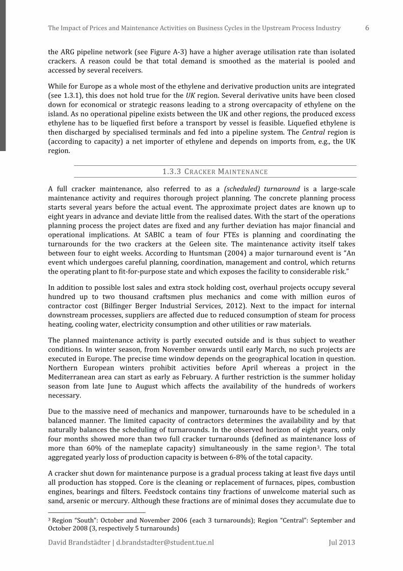
A full cracker maintenance, also referred to as a (scheduled) turnaround is a large-scale maintenance activity and requires thorough project planning. The concrete planning process starts several years before the actual event. The approximate project dates are known up to eight years in advance and deviate little from the realised dates. With the start of the operations planning process the project dates are fixed and any further deviation has major financial and operational implications. At SABIC a team of four FTEs is planning and coordinating the turnarounds for the two crackers at the Geleen site. The maintenance activity itself takes between four to eight weeks. According to Huntsman (2004) a major turnaround event is “An event which undergoes careful planning, coordination, management and control, which returns the operating plant to fit-for-purpose state and which exposes the facility to considerable risk.”
In addition to possible lost sales and extra stock holding cost, overhaul projects occupy several hundred up to two thousand craftsmen plus mechanics and come with million euros of contractor cost (Bilfinger Berger Industrial Services, 2012). Next to the impact for internal downstream processes, suppliers are affected due to reduced consumption of steam for process heating, cooling water, electricity consumption and other utilities or raw materials.
The planned maintenance activity is partly executed outside and is thus subject to weather conditions. In winter season, from November onwards until early March, no such projects are executed in Europe. The precise time window depends on the geographical location in question. Northern European winters prohibit activities before April whereas a project in the Mediterranean area can start as early as February. A further restriction is the summer holiday season from late June to August which affects the availability of the hundreds of workers necessary.
Due to the massive need of mechanics and manpower, turnarounds have to be scheduled in a balanced manner. The limited capacity of contractors determines the availability and by that naturally balances the scheduling of turnarounds. In the observed horizon of eight years, only four months showed more than two full cracker turnarounds (defined as maintenance loss of more than 60% of the nameplate capacity) simultaneously in the same region3. The total aggregated yearly loss of production capacity is between 6-8% of the total capacity.
A cracker shut down for maintenance purpose is a gradual process taking at least five days until all production has stopped. Core is the cleaning or replacement of furnaces, pipes, combustion engines, bearings and filters. Feedstock contains tiny fractions of unwelcome material such as sand, arsenic or mercury. Although these fractions are of minimal doses they accumulate due to 3 Region “South”: October and November 2006 (each 3 turnarounds); Region “Central”: September and October 2008 (3, respectively 5 turnarounds)

7 Introduction to the Petrochemical Industry
Master Thesis TU/e Eindhoven
the high material throughput and clog appliances reducing their throughput capability. This process is called fouling. Next to fouling, petroleum coke is a trigger for maintenance. Furnaces need to be decoked every 40 to 60 days aside of the turnaround schedule in order to maintain high thermal transition.4
Cracker turnaround processes have received increasing attention in Europe which led to considerable efficiency gains and a significant difference in total turnaround duration of Europe compared to other regions. Horizontal collaboration in the sense of knowledge transfer and best practice exchange between competitors takes place. The IQPC organises an annual conference on shutdowns and turnarounds (IQPC, 2013).
The common interval of six years for major turnarounds is legislation driven. The period got extended recently and used to be four years. Main concerns from a legislation point of view are safety and environmental issuess. It is technically possible to extend the six year period even further as the technical driver of turnarounds, the fouling, can be hampered longer. Yet it is said that the organisational effort to manage the workers and maintenance processes is an upper bound for the extension of maintenance activities.5
It is not possible to buffer the full production loss during a cracker outage by building up stocks beforehand. SABIC has a combined stock capacity at its Geleen site for several days of ethylene production and a capacity of a few weeks in the UK due to underground storage in cavities. Thus, manufacturers purchase material from competitors to secure supply during a turnaround. At the same time, utility providers have been informed well in advance to adjust their supplies as well. Product sourcing for the turnaround period usually takes place worldwide. It is estimated that the physical costs of a turnaround (contractors) are of the same magnitude as the production profit loss. An alternative or supplemental strategy to purchases from competition, which can only be chosen in times of excess capacity, is to overproduce ethylene in order to produce polyethylene with the purpose of stocking it. The cracker activities are reported in detail (expected extent and month) in industry reports like those provided by IHS/CMAI (2005-2013) around six months prior to the event.
In addition to planned maintenance also unplanned maintenance is reported. Although aggregated exceeding the capacity loss of planned maintenance activities, unplanned outages are usually on a smaller scale per unit in contrast to a turnaround. Unplanned outages typically affect only a small number of furnaces whereas a turnaround is eventually affecting all of them. A complete unexpected shutdown of a cracker happens but is, also due to careful maintenance and high safety standards, very rare6.
A correlation analysis of the unplanned dataset showed spurious significant relationships with e.g. oil price and GDP growth7. Thus, it can be supposed that a (severe) market-driven capacity reduction is reported as technical maintenance loss and thus biasing the dataset. Next to price volatility of naphtha (see 1.4.2) and ageing polymer production tools (see 1.3.2), “too frequent production stops and ‘forces majeures 8 ’ for production breakdowns and emergency maintenances” are the biggest concern of the downstream converter industry (Packaging Europe, 2013). 4 The decoking is also the reason why a cracker hardly ever reaches its nameplate capacity. On average 1-3 furnaces are offline for decoking at any time. 5 The amount of tasks can be estimated to grow linearly with the length of the maintenance interval. 6 Naphtachimie’s Lavera cracker had to be shut down completely in December 2012 due to a fire (ICIS news, 2013). 7 Crude Oil (second period): 𝑟 = −0.256 sig: 0.04. GDP growth (first period): 𝑟 = −0.223 sig: 0.064. 8 “Force majeure […] is a common clause in contracts that essentially frees both parties from liability or obligation when an extraordinary event or circumstance beyond the control of the parties […] prevents one or both parties from fulfilling their obligations under the contract.” (Wikipedia, 2013).

The Impact of Prices and Maintenance Activities on Business Cycles in the Upstream Process Industry 8
David Brandstädter | [email protected] Jul 2013
1.4 PRICES AND CONTRACTING
Karl Marx had a less profound definition of commodities when he stated that “one can not [sic] tell by the taste of wheat whether it has been raised by a Russian serf, a French peasant or an English capitalist.” (Boudin, 2008, p. 56). As one can certainly discuss if food from one source is truly substitutable by food from another one, this is not true for commodity products in the petrochemical industry. Products like propylene, ethylene or feedstock types such as propane and ethane have to qualify for certain grades but are perfectly interchangeable between players. For naphtha the picture looks a bit different as the amount of crude oil, condensates and particles like sand or metals can vary.
For producers, this means that they cannot compete on product quality and are highly exposed to price risk. Whereas crude oil and naphtha prices recently reached nearly three times their 1990 value, the polyethylene price corrected for inflation never reached its 1990 level. Likewise, the important polyethylene/naphtha spread declined to half 1990 value. This spread depicts the upper bound of the margin of polyethylene producers who purchase naphtha to produce and sell polyethylene. All four prices show very high and significant correlations with Pearson coefficients of 0.95 and higher (see Table C-2).
Upstream producers are facing additional exposures as a result of properties of chemical processes: To ensure constant operation, the price sensitivity of players on the upper part of the stream is relatively low (due to low storage capacity, feedstock has to be purchased regardless of the current price to prevent production starving) whereas further downstream price sensitivity increases (storage ability increases, customers can partly commit in pre or delayed buying).
FIGURE 8: COMPOSITION OF CRUDE OIL DERIVATES IN EUROPE
It is important to understand that only a relatively small amount of crude oil discharged in Europe ends up in the petrochemical industry. Estimates for 2012 account 8% of crude oil to be processed into naphtha of which around half is used as feedstock for the petrochemical industry, representing 4% of the overall crude oil volume (see Figure 8). Thus, it can safely be assumed that naphtha is highly dependent on crude oil price and relatively insensitive to ethylene or polyethylene demand.
1.4.1 CONTRACT AND SPOT SALES
The majority of polyethylene sales are done by contracts. Contract prices are settled once a month and reported to the market. Discounts of several percentage points on the settled contract price are common but limited. Contracts exist in high variety in terms of volumes,
Crude oil (100%)
Diesel (44%)
Residual Fuel (22%)
Gasoline
Jet fuel Naphtha
LPG (3%)
Petrochemicals (4%) 13%
10% 8%
~ 50%
Typical derivative fraction of crude oil
Barrel [North West Europe] Source: CERA/CEFIC (2012), Internal estimation
9 Introduction to the Petrochemical Industry
Master Thesis TU/e Eindhoven
reference prices, discounts, delivery dates and termination dates. The contract horizon can vary between 1 and 15 years with a tendency towards the shorter side. Contracts hardly ever have a fixed price. Instead, a price formula depending on the settled market contract price (CP) is stated. Hence, contracts still include a substantial amount of uncertainty regarding price but ensure an outlet for volume.
As stated in 1.3.1 ethylene and polyethylene production is integrated. Only a very low amount of total production is traded on the spot market. Despite being a contract business, the spot market for polyethylene is relatively liquid and spot opportunities are seized.
1.4.2 INCREASED PRICE VOLATILITY
The prices for naphtha, ethylene and polyethylene were subject to increased volatility over the last years. Values outside a confidence band of ±1 standard deviation of the linear trend over a long time period are said to show “unusual price activity.” (Hodges, 2010). Peak and through of the “Lehman Wave” (Peels, et al., 2009) in 2008 and 2009 broke this band twice (n.b. on both bands). Since then the upper threshold was surpassed once more for naphtha and three times for polyethylene. The slope of the linear trend of naphtha is larger than the one for polyethylene resulting in a negative linear long-term trend for the price spread. In other words, the upper bound for the polyethylene producers’ margin has been shrinking on a linear trend level since 1990.
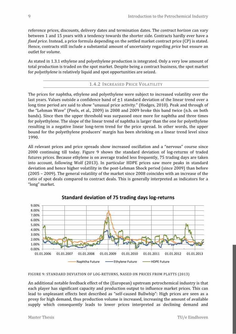
All relevant prices and price spreads show increased oscillation and a “nervous” course since 2000 continuing till today. Figure 9 shows the standard deviation of log-returns of traded futures prices. Because ethylene is on average traded less frequently, 75 trading days are taken into account, following Wolf (2013). In particular HDPE prices saw more peaks in standard deviation and hence higher volatility in the post-Lehman Shock period (since 2009) than before (2005 – 2009). The general volatility of the market since 2008 coincides with an increase of the ratio of spot deals compared to contract deals. This is generally interpreted as indicators for a “long” market.
FIGURE 9: STANDARD DEVIATION OF LOG-RETURNS, NASED ON PRICES FROM PLATTS (2013)
An additional notable feedback effect of the (European) upstream petrochemical industry is that each player has significant capacity and production output to influence market prices. This can lead to unpleasant effects best described as “self-caused Bullwhip”: High prices are seen as a proxy for high demand, thus production volume is increased, increasing the amount of available supply which consequently leads to lower prices interpreted as declining demand and
0.00%1.00%2.00%3.00%4.00%5.00%6.00%7.00%8.00%9.00%
01.01.2006 01.01.2007 01.01.2008 01.01.2009 01.01.2010 01.01.2011 01.01.2012 01.01.2013
Standard deviation of 75 trading days log-returns
Naphtha Future Ethylene Future HDPE Future

The Impact of Prices and Maintenance Activities on Business Cycles in the Upstream Process Industry 10
David Brandstädter | [email protected] Jul 2013
eventually a reduction of production. Likewise, long markets with supply exceeding demand lead to price reduction in order to find sufficient outlets. Due to the extensive delays stemming from continuous production, follow-up supply in subsequent periods is facing even less demand leading to even lower prices. Eventually, capacity reduction will kick in as attempt to balance supply and demand. The same delay effect will lead to inflated prices once demand is picking up again.
1.5 THE SUPPLY CHAIN OF PLASTICS
The plastic supply chain consists of four relevant production steps. Crude Oil refinery is an important fifth step but its main purpose is the production of gasoline, heating oil or kerosene. Naphtha, the main input for the European plastic production, can be classified as by-product of crude oil refinery (see Figure 8). As described in 1.3, Cracker Units split up the long-carbon chains in naphtha to transform it to ethylene next to a high variety of other products. The ethylene is used by Polymer Units to produce polyethylene in different grades. Polyethylene is shipped to converters which use different techniques such as blow or injection moulding to produce plastic packages, pipes and films. Traders sometimes act as intermediary by taking a stock position and utilise price fluctuations or act as distributors to smaller converters. The plastic product is then sold to OEM businesses that use it for applications or packaging before a final product is shipped to consumer end markets such as food.
close integration
4Cracker
Units
3Polymer
Units
2 Converters
1OEMs
CrudeOil Refineries
Consumer End
Markets
Naphtha Ethylene Poly-ethylene
Plasticproduct
Finalproduct
Traders
FIGURE 10: GENERIC PLASTIC SUPPLY CHAIN FOR POLYETHYLENE
1.5.1 PLAYERS IN THE VALUE CHAIN
As stated in 1.1 the petrochemical business, specifically the echelon 4 and 3 are dominated by large global players often covering both production steps, ethylene and polyethylene production. In case the two production steps are executed by two different companies (see 1.1.1), long-term contracts secure an outlet and lead to a “quasi integrated” constellation.
Further down the stream, the landscape of supply chain players becomes more scattered. Converters are often relatively small companies with an average of 26 FTEs per company (European Plastics Converters, 2010). However, recent developments show a trend for consolidation, increasing purchasing and negotiation power of converter companies, especially in northwest Europe. Bigger companies have a more robust cash flow position as well as higher storage capabilities and thus can engage into forward or delayed buying.
Likewise, converters face increasingly volatile demand. With exceptions in the automotive and construction industry, plastic applications are rarely an essential or particularly valuable part of a final product. Some of the larger OEMs negotiate directly with plastic producers and bypass the converters to some extent. In general, converters are seen as “the weakest link” in the (plastic) chemical supply chain.

11 Introduction to the Petrochemical Industry
Master Thesis TU/e Eindhoven
1.5.2 TRANSPORT AND INVENTORY
Throughout the supply chain all major modes of transportation are used. Naphtha as feedstock for cracker units is mainly transported by liquid bulk vessels. Ethylene is the most sensitive intermediate product to transport from a safety perspective due to pressure and high flammability. With a boiling point of -103.8 °C (Air Liquide, 2013), ethylene is preferably stored gaseous. For pipeline transport, the gas is set to its supercritical state by high pressure (ca. 100 bar) so that it shows desirable characteristics of a fluid. In case pipeline transport is not available, ethylene is liquefied and shipped in specialised high-pressure vessels (see situation in the UK, 1.3.2). Because of its chemical properties, ethylene is stored as little as possible. Storage capacity is very limited. A special role plays the high pressure gaseous storage in underground salt cavities practiced in the UK (British Geological Survey, 2008).
Derived polyethylene is easily storable and shipped either as dry bulk or in containers. Polyethylene inventory can be and are being used to buffer against price uncertainty or to take a speculative motivated position. Stocks are held by producers and customers. Remarkable fluctuations could be observed before the Lehman Shock followed by period of rather tightly managed stocks. Since late 2011, stocks are fluctuating considerably again.
Plastic products manufactured by converters are then typically shipped by truck or bulky goods transport (e.g. pipes). Order characteristics of OEM vary according to the application of the plastic product. High-frequent deliveries are common for dedicated mass products, in particular in the food industry. General packing products are often ordered infrequent to stock.
1.5.3 GLOBAL MARKET
Both world and European market have faced increasing trade activity (see Figure 11). Europe is in- and exporting polymers worldwide. Generally, imports to Europe of simple pure commodity grades manufactured by a large number of manufacturers have increased. Rather specialised, high-technology polymer grades (e.g. multilayer, lightweight – see 1.1.2) have seen increasing exports. The European polymer market can be seen as the most advanced with regards to technology. Over the last years, technology enhancement has reached polymer products with former commodity characteristics. Cheap imports cannibalise market shares of low-tech products which forces European manufacturers to engage in high-value products.
FIGURE 11: RELATIVE POLYETHYLENE TRADE AND PRODUCTION GROWTH OF EU25 (EUROSTAT, 2013)
0%
50%
100%
150%
200%
250%
'99 '00 '01 '02 '03 '04 '05 '06 '07 '08 '09 '10 '11 '12
Polyethylene trade and production growth (EU 25)
Extra EU Import [kt]
Extra EU Export [kt]
Production [kt]

The Impact of Prices and Maintenance Activities on Business Cycles in the Upstream Process Industry 12
David Brandstädter | [email protected] Jul 2013
1.6 PROJECT LAYOUT
The study was conducted within the 4C4Chem industry project, funded by participating companies and subsidised by the Dutch Institute for Advanced Logistics, DINALOG under the lead of the Technical University Eindhoven, TU/e. The goal is to achieve mutual benefits in terms of cost, efficiency and environmental footprints. This work contributes by increasing mid-term price and demand forecasting quality.
The operational part including interview and data collection was preceded by a literature review and a research proposal. Goals were aligned to satisfy both industry and academia interests. The study aims to balance aspects of relevance by focusing on tool implementation and aspects of rigour by using general models as well as assessing generalizability of the work.
Expansive scoping decisions had to be made to ensure feasibility and adequate level of detail. Those are discussed in section 1.6.1. Comments on how data was collected and used are made in 1.6.2. The detailed research methodology is laid out in 3.3.
1.6.1 PROJECT SCOPE
The chemical value chain is extremely divergent, expanding quickly from a few raw materials like crude oil and natural gas, to thousands of product branches including plastics, rubbers, solvents and vinyl. SABIC’s portfolio is covering a relatively large amount of those variety. However, ethylene and the derived polyethylene comprise the largest volume of SABIC and the European production market. Further, cracker units are usually operated by an optimisation function based on ethylene. Consequently, the volume of contingent by-products is predetermined.
Three different product groups of polyethylene are produced: High density polyethylene (HDPE), low density polyethylene (LDPE) and low linear density polyethylene (LLDPE). Figure 12 shows that all three products together account for more than half of the derivatives from ethylene.
FIGURE 12: USE OF ETHYLENE IN EUROPE PER PRODUCT (APPE, 2012)
Further, the approach of previous work (Udenio, et al., 2012), (Corbijn, 2013) to aggregate data to a market level is followed. An echelon in the model thus represents competing companies. This choice was made to better capture high-level trends and structural as well as dynamic effects on an industry rather than a single firm level. For the statistical models, higher aggregation level lowers the probability of measurement errors and impact of outliers (Arya, 2004).
24%
22%
13%
14%
11%
7% 7%
1% 1%
European ethylene consumption (2012)
HDPELDPELLDPEEDCEthylene OxideOthersEthyl-benzeneAlpha-OlefinsVinyl Acetate

13 Introduction to the Petrochemical Industry
Master Thesis TU/e Eindhoven
Although traders present an interesting role in terms of supply chain finance, their overall impact on the industry is currently relatively small (see 1.5.1) and thus traders are put out of scope. Relevant end markets were again chosen based on volume and are described in detail in Chapter 5.
The introduction showed structure and characteristics of the supply chain of plastics. The upstream industry was facing increased volatility in recent years. This study is using a quantitative modelling approach to partly answer the research question what are the reasons for high demand fluctuations in the petrochemical supply chain?
Recent literature discussed in Chapter 2 already gives indication for the underlying reasons and a first step towards a systematic explanation. In Chapter 3, detailed research questions are phrased aiming at closing identified gaps in the literature and following up findings of the introduction.
1.6.2 PROJECT APPROACH
The data and information gathering for the study relied on expert interviews combined with market reports and database services. Table 1 lists the relevant sources and nature of data.
TYPE OF DATA SOURCE NATURE OF DATA
Expert interviews SABIC Chemicals, SABIC Polymers, TU/e Eindhoven quantitative/qualitative
Industry Reports IHS/CMAI Europe/Middle East Light Olefins Market Advisory Service, Confidential quantitative/qualitative
Database services IHS Global Insight, IHS Chemicals, Eurostat quantitative
S&OP SABIC Chemicals, SABIC Polymers quantitative
TABLE 1: OVERVIEW OF USED DATA SOURCES
The Impact of Prices and Maintenance Activities on Business Cycles in the Upstream Process Industry 14
David Brandstädter | [email protected] Jul 2013
2 LITERATURE REVIEW
This chapter gives a brief overview of supply chain dynamics including applications of the System Dynamics modelling technique and commodity price volatility. The last section lists identified gaps relevant for the conducted study.
2.1 SUPPLY CHAIN DYNAMICS
The concept of System Dynamics, initially called ‘Industrial Dynamics’, was developed in the mid-1950s by Forrester (1961). Motivated by his field-experience with industry managers he claimed that “the biggest impediment to progress comes, not from the engineering side of industrial problems, but from the management side […]” because “social systems are much harder to understand and control than are physical systems.” (System Dynamics Society, 2013). System Dynamics “links together hard control theory with soft system theory” (Fiala, 2005) and has been used frequently to model aggregated supply chains in order to analyse the system’s performance, policies and human behaviour. In a review paper Riddalls et al. (2000) attribute dynamic simulation better insight into strategic and global behaviour of supply chains than traditional operations research techniques focusing on tactical control and optimisation. The authors in particular criticise the lack of thorough sensitivity analysis in models of the latter group.
Likely the System Dynamics paper recently attracting most attention in the area of supply chain management is Sterman’s application of a decision making heuristic on the beer game (Sterman, 1989). System Dynamics has been the method of choice for numerous studies on the Bullwhip Effect. Wikner et al. (1991), although not using the term “Bullwhip”, used System Dynamics to identify and mitigate sources of demand amplification. Disney & Towill (2003) investigated the effect of VMI on the Bullwhip Effect using System Dynamics. Tako & Robinson (2012) reviewed 18 System Dynamics papers on the Bullwhip Effect accounting for 18% of all System Dynamics papers in logistics and supply chain management published in peer reviewed journals between 1996 and 2006. In contrast, only five papers discussing the Bullwhip Effect using DES, 2% of all DES-literature were identified. Whereas the presence of the Bullwhip Effect is widely acknowledged, its measurement is in disaccord. Fransoo & Wouters (2000) define the bullwhip effect as ratio of variation created by an echelon (or aggregated set of echelons) and variation faced by this echelon at its inbound. They advise great care when measuring the effect such as the right level of aggregation and adequate use of filters. Cachon et al. (2007) claim that “strong forces mitigate the” Bullwhip Effect and thus it often cannot be observed in industry data. Lee et al., who coined the term Bullwhip Effect and gave an initial definition (Lee, et al., 1997), argue in a response to Cachon’s work (Chen & Lee, 2012) that one has to distinguish information flow (e.g. orders, forecast) from material flow (inventories, shipments) and further has to pay attention to the level of aggregation (product, time).
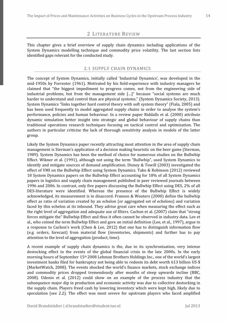
A recent example of supply chain dynamics is the, due to its synchronisation, very intense destocking effect in the events of the global financial crisis in the late 2000s. In the early morning hours of September 15th 2008 Lehman Brothers Holdings Inc., one of the world’s largest investment banks filed for bankruptcy not being able to redeem its debt worth 613 billion US-$ (MarketWatch, 2008). The events shocked the world’s finance markets, stock exchange indices and commodity prices dropped tremendously after months of steep upwards incline (BBC, 2008). Udenio et al. (2012) could show on an example of the process industry that the subsequence major dip in production and economic activity was due to collective destocking in the supply chain. Players freed cash by lowering inventory which were kept high, likely due to speculation (see 2.2). The effect was most severe for upstream players who faced amplified

15 Literature Review
Master Thesis TU/e Eindhoven
oscillation around the long term economic cycle. Udenio et al. used a high-level System Dynamics model of the aggregated supply chain to describe the substantial effects which were summarised as “Lehman Wave”. Recently, a linear control theory approach has been used to investigate the system performance of such behavioural response on a demand shock and to confirm the findings with the help of a different modelling technique (Udenio, et al., 2013).
Disney et al. (2006) argue that differential equations, the mathematical fundament of System Dynamics, in combination with continuous time are more suitable to analyse such oscillation behaviour of a supply chain, than difference equations on a discrete time function. Angerhofer & Angelides (2000) categorise System Dynamics research in the field of supply chain and operations management in three different groups: 1) research concerned with contributing to theory-building, 2) research using System Dynamics Modelling to solve a problem and 3) research work on improving the modelling approach. The System Dynamics part of this study can be classified as problem solving with elements of theory building by applying established models in a partly new environment and thus building new evidence, in particular for the “Lehman Wave” phenomenon. By comparing two periods of the same data set, insights in factors concerning calibration are given and hence the study contributes to an improved modelling approach as well (see Figure 13).
Theory building
Improving modelling approach
Problem solving
FIGURE 13: POSITION OF THE STUDY IN TAXONOMY TRIANGLE BY ANGERHOFER & ANGELIDES (2000)
2.2 COMMODITY PRICING AND VOLATILITY
The decade 2002 to 2012 has been coined “super cycle” by commodity price observers (CNBC, 2013). In 2002 demand began to recover from the burst of the new economy bubble and quickly ran ahead of the supply side which had faced severe divestments due to the 2001 recession (see Figure 14). Low inventories led to price growth. Due to delay in capacity investment, price continued rising. After new investments kicked in, capacity growth exceeded consumption growth eventually leading to balanced or surplus markets. This equilibrium is suspected to have been reached in early 2008 (Hodges, 2010). The reason for further price incline throughout the remainder of 2008 is still not fully understood but clearly shows behaviour of a bubble caused by speculation (Khan, 2009).
From a supply chain point of view, a reason enhancing commodity price swings is the fast and prompt price pass-through from upstream commodities to downstream products. Whereas in 2004 representative supply chains showed a price-lag of 5 months, this has been diminished to one month and less (IHS, 2012).

The Impact of Prices and Maintenance Activities on Business Cycles in the Upstream Process Industry 16
David Brandstädter | [email protected] Jul 2013
FIGURE 14: GLOBAL INSIGHT INDUSTRIAL MATERIALS PRICE INDEX (HODGES, 2010)
Dvir and Rogoff (2010) investigate the relationship of storage and crude oil price. Stocks are willingly increased when future price corrected for holding and credit costs is expected to be higher than present price. Is the access to excess supply restricted, this storage behaviour increases price volatility. Kilian & Murphy (2010) also focus on inventories to explain recent oil price shocks. They argue, however, that the strong increase of real oil price between 2003 and 2008 as well as its collapse and partial recovery is driven by shifts in consumption rather than speculative demand. In the aftermath of the recent financial crisis, many hold speculative futures trading responsible for volatility (e.g. Singleton (2011)). While admitting that speculative behaviour such as reacting to news about prospective supply accounts for “part of the recent volatility”, Bernanke (2004) states, n.b. prior to the Lehman bankruptcy, that “available evidence does not provide clear support for the view that speculative activity has made oil prices during the past year much higher on average than they otherwise would have been”. Greenspan (2004) concludes that “much of world oil supplies reside in potentially volatile areas of the world”. However, also to date, almost five years after the default, research is still divided over the impact of speculation on oil prices (Wigan, 2012) and (Fattouh, et al., 2012). Older work is suggesting that the special role of controlled supply as enforced by OPEC is the reason behind higher volatility of oil price compared to other commodities such as metals and wheat (Plourde & Watkins, 1998). Hornstein (1998) suggests that fluctuations in inventory cannot explain output fluctuations over the business cycle but “are important for short-term output fluctuations.”. No literature could be identified discussing ethylene prices. Whereas ethylene highly depends on naphtha and hence crude oil both process and price wise, the demand side for plastics is decoupled from the energy and transportation demand crude oil is satisfying.
2.3 IDENTIFIED GAPS
The process industry has been subject to several studies using a linked single-echelon model. To date, no study is known using System Dynamics including the cracker echelon as first step in the plastic value chain.
Price effects on orders have been investigated before (Corbijn, 2013) but not on a feedstock level and neither on an individual product stream basis.
The matter of maintenance in the process industry has been addressed in scheduling problems (Berning, et al., 2002) but not concerning large-scale cracker turnarounds. Moreover, the effect on prices was not investigated before. In general the focus in literature discussing seasonal supply chains has been on the demand side of the chains. Recognised work on “seasonal capacity” is not known of.

17 Research Contribution
Master Thesis TU/e Eindhoven
3 RESEARCH CONTRIBUTION
The contribution to research is threefold: First, additional evidence is built for the relatively new concept of the Lehman Wave. Current work covering the process is extended on the supply side by increasing scope to one additional echelon upstream (ethylene production) and on the demand side by investigating three distinct polymer products. Second, factors to improve the System Dynamics modelling approach on complex supply chains are discussed. Findings are presented underlying the importance of carefully selecting the starting point of calibration. Third, factors not being discussed in literature yet, such as the influence of large-scale maintenance on the supply chain and on price, are investigated.
A contribution focusing on application in practice is the development of a structural forecast model in contrast to widely used time-series based forecast techniques. The latter ones by definition lag behind actual data and cannot predict turning points. A structural model takes into account inventory levels as well as material and information delays which allows it to predict such turning points.
3.1 PROBLEM STATEMENT
Crackers and subsequent production units are operated in a strong push manner from upstream towards downstream echelons with little knowledge of the supply chain behaviour and consideration of end market demand. The impact of own and competition’s facility outages on business cycles and prices is not fully understood. Likewise, the relationship between business cycles and commodity pricing as well as feedstock prices is not fully understood or incorporated into planning decisions. Observed demand shows significantly higher volatility following the Lehman Shock and price sensitivity of customers has increased and is reflected in order patterns. In case of excess production, prices have to be lowered considerably to “push” the product into the market thus eroding margins and partake in next period’s demand.
Moreover, since the Lehman Shock demand forecast quality has decreased substantially. Incorrect planning and operating decisions can lead to disadvantageous purchases, sales and contracting caused by prevention of bottleneck starving or blocking.
3.2 RESEARCH QUESTIONS
From the problem statement discussed in 3.1 and the introductory chapter as well as the literature review, two main research questions can be derived. This chapter presents both research questions and brief explanations.
RESEARCH QUESTION 1:
What are the underlying structural reasons in petrochemical supply chains causing high fluctuations experienced at the demand side of upstream players and what is the nature of the caused effects?
Observed demand volatility has increased since the Lehman Shock although the structure of European supply chains has not changed significantly. Structural reasons could be the lack of storing capacity and capability upstream, the strong integration of production units, but also the

The Impact of Prices and Maintenance Activities on Business Cycles in the Upstream Process Industry 18
David Brandstädter | [email protected] Jul 2013
limitation in adjusting production volume, the general overcapacity in the market and the unknown stock capacity of downstream echelons.
Further, extra-European imports of derivative products like HDPE, LDPE and LLDPE recently increased and further augment pressure on local margins. As a last point, the inherited push characteristic of upstream parties could qualify as a structural reason as well (although showing dynamic aspects, too - see Research Question 2).
After having identified reasons for demand fluctuation, the direction, magnitude and characteristic – the nature – of the effects they cause, is of interest.
RESEARCH QUESTION 2:
How do underlying dynamics in petrochemical supply chains facilitate and amplify these observed fluctuations on demand and supply side?
Identified dynamics are on the one hand, the strong impact of commodity and feedstock prices on observed order behaviour and production volumes. On the other hand, large maintenance activities such as cracker outages have a significant effect on commodity price spreads and explain a substantial part of its variance. They act on two directions of the chain: As a capacity constraint and by that as limiting factor on demand, as well as on prices and by that as a disrupting factor of demand.
Both research questions imply certain investigative steps. However, a particular primary question withholds a clear answering strategy and is thus listed separately with the aim of being answered throughout the project by findings related to the answer of the research questions above:
What is an adequate demand proxy in the petrochemical industry?
The motivation for this question is whether a sole price observation is sufficient to describe demand patterns or if it needs to be extended and linked to volume levels. In particular the increased price volatility (see 1.4) and price sensitivity of converters (see 2.2) suggests an enlarged impact of buying strategies not directly linked to end-market demand.
3.3 RESEARCH METHODOLOGY
This work is based on two conceptually independent models each addressing a different angle of the research questions as stated in 3.2: A Maintenance-Price Regression Model and a Basic Supply Chain Model based on System Dynamics. Structure and findings of both models are then combined in an Advanced Supply Chain Model. Figure 15 illustrates the framework.
Maintenance-Price Regression Model (Chapter 4)
This statistical model investigates the relationship between cracker maintenance activities and commodity price spreads. In a multiple linear regression model the extent of maintenance activities, the oil price and quarterly GDP growth are used to explain the price spreads of ethylene/naphtha as well as polyethylene/naphtha. A multiple regression model is used because it matches the objective of predicting “changes in the dependent variable in response to changes in the independent variables.” (Hair, et al., 2009, p. 17). Further, only one dependent variable (price spread) is considered, it is a metric variable and the size is of interest. All of which are requirements for a multiple regression analysis.

19 Research Contribution
Master Thesis TU/e Eindhoven
FIGURE 15: RESEARCH MODEL STRUCTURE
In an extension the forecast ability is enhanced by using historical dependent variables instead of data from the same time period. Monthly benchmark reports of the industry are used to derive the maintenance data. Prices are extracted from information provider databases (IHS/CMAI, 2005-2013).
Basic Supply Chain Model (Chapter 5)
The basic supply chain model is similar to the one discussed by Udenio et al. (2012) who based their model on Sterman’s One-Echelon Model (2000, pp. 709-755). It is extended by an order release function and a capacity limitation as an effect of cracker maintenance. System

The Impact of Prices and Maintenance Activities on Business Cycles in the Upstream Process Industry 20
David Brandstädter | [email protected] Jul 2013
Dynamics has been used frequently to model supply chain dynamics such as Bullwhip and synchronised destocking effect. A forecast feature is implemented and the extension of incorporating capacity limitation and product imports evaluated. In addition to forecast applications the model allows for precise policy or scenario analysis, the very core of System Dynamics modelling (Forrester, 1961).
The model uses end market demand data (Eurostat, 2013) and is calibrated against observed production output of crackers, the highest echelon.
Advanced Supply Chain Model (Chapter 6)
The advanced supply chain model is in its core the basic model extended by a stock effect. The stock effect adjusts an echelon’s order volume according to observed price movements based on previous studies (Corbijn, 2013). This price response is introduced at the converter Echelon 2 for all three different product streams (HDPE, LDPE, and LLDPE). In addition, the response is also introduced for feedstock purchases of the cracker Echelon 4.

21 Maintenance-Price Model
Master Thesis TU/e Eindhoven
4 MAINTENANCE-PRICE MODEL
Cracker turnarounds affect operations and planning in a reoccurring pattern which led to the establishing of best practice processes across the industry. The effect on feedstock and product prices is, however, less well understood. Sales management and business intelligence agree that there “is an effect on prices” but this effect has not been quantified yet. Turnarounds are reported as part of a monthly industry overview report listing “loss of capacity in kilo tons ethylene”. They are thus not listed as binary but as a planned nominal capacity loss. Next to the reported planned figures, also unplanned maintenance is reported to the industry. However, due to the fact that market product prices are settled on a monthly basis (see 1.4) short-term capacity losses are expected to have little influence on monthly prices. As further discussed in 1.4, the monthly settled contract price is only a guideline for producers and firm-specific discounts can be and are applied. This is where a short-term maintenance activity could be reflected, but remains unnoticed by industry reports.
In order to isolate this abovementioned effect of (planned) maintenance activities on prices one first has to understand the influence of it on the planning process of different products. As shown in Figure 5 and discussed in 1.6.1, ethylene is the most important cracker product in terms of volume. Planning decisions in production are mainly driven by ethylene and its derivatives. The production volumes for other by-products are determined by ethylene. Hence, as ethylene is the most relevant product for planning and, due to its far-reaching impact (see 1.3.3), scheduled maintenance is taken into account in planning decisions, maintenance activity is expected to have an effect mainly and strongest on ethylene and derivative prices. Because capacity is taken out of the market, supply availability decreases. Assuming an independent demand, this creates a short market situation. Because naphtha price can be seen exogenous (see 1.4), the ethylene as well as polyethylene prices are expected to rise which eventually leads to a widening of the relevant price spreads and the following hypothesis:
HYPOTHESIS 1A: MAINTENANCE ACTIVITIES OF CRACKER UNITS HAVE A POSITIVE EFFECT ON PRICE SPREADS OF COMMODITY PRODUCTS.
Figure 16 summarises the hypothesis and the corresponding model steps which are used to confirm the premise. In 4.1 the hypothesis is further detailed and the statistical model explained. 4.2 then investigates the practical implications, namely the influence on customer order behaviour.
FIGURE 16: HYPOTHESIS ARGUMENT AND CORRESPONDING MAINTENANCE-PRICE MODEL
Hypothesis
Due to high volume share, ethylene price spread is affected the most by cracker maintenance.
Because of its strong impact on capacity, maintenance can explain a substantial part of the price variance.
Due to long-term planning of cracker turnarounds, the model can be extended to forecast price spreads.
Model
1) Correlation analysis (maintenance on price spreads)
2) Regression analysis (maintenance, oil price and GDP to predict product price spreads)
3) Extended lagged regression analysis (adaption for historic oil prices)

The Impact of Prices and Maintenance Activities on Business Cycles in the Upstream Process Industry 22
David Brandstädter | [email protected] Jul 2013
4.1 EFFECT ON PRICE SPREADS
For the analysis a dataset has been composed using past industry reports on cracker outages (IHS/CMAI, 2005-2013). The set was split up in two equal parts, one before the big demand collapse and one right after. As discussed in 1.1.1, the shockwave after the Lehman Brother’s bankruptcy had severe consequences for the European industry and thus justifies a split up. The data for the maintenance activities is aggregated on a European industry level per months and gives 94 entries of the variables unplanned maintenance and planned maintenance for each set.
4.1.1 CORRELATION ANALYSIS
It is assumed that a maintenance activity on the cracker production unit firstly and strongest affects prices of products which are manufactured in a cracker. Based on volume these are ethylene, propylene, benzene and butadiene (see Figure 5). The variables listed in the rows of Table 2 are common contract and spot market prices9,10 for those products, either at a terminal or out of a pipeline.
As discussed in 2.2, commodity prices of the plastic value chain are highly correlated with each other (cross-correlation) and with themselves (auto-correlation). This poses a problem for regression analysis because it violates the ordinary least squares assumption that the error terms are uncorrelated and can lead to inflated R²-values (Field, 2005). Thus the reported prices for ethylene, propylene, benzene and butadiene are in fact price spreads of the listed price minus the CIF naphtha price. Using spreads is common for analyses conducted in the petrochemical industry. Table C-2 shows the strong correlation of products throughout the plastic value chain, Figure 17 illustrates the difference in auto-correlation of absolute prices and price spreads.
FIGURE 17: AUTOCORRELATION OF PRICES FOR NAPHTHA, TTHYLENE AND PRICE SPREAD
Quarterly GDP growth and crude oil price are commonly used to predict plastic product prices. Including them in this correlation analysis as “control” variables serves two purposes: First, it is tested if both variables can be used in combination with the planned maintenance variable for regression analysis where uncorrelated predictor variables are favourable. Second, a correlation between maintenance activities and GDP growth (respectively crude oil price) would indicate a 9 Incoterm CIF: Cost, Insurance, Freight: “Seller must pay the costs and freight to bring the goods to the port of destination. However, risk is transferred to the buyer once the goods are loaded on the vessel. In addition, seller must procure and pay for the insurance. Maritime transport only.” (Wikipedia, 2013). 10 Incoterm FOB: Free on Board: “Seller pays for transportation of goods to the port of shipment, loading cost. The buyer pays cost of marine freight transportation, insurance, uploading and transportation cost from the arrival port to destination. The passing of risk occurs when the goods pass the ship's rail at port of shipments.” (Wikipedia, 2013).

23 Maintenance-Price Model
Master Thesis TU/e Eindhoven
flawed dataset as it can safely be assumed that both variables are not influencing the long planned maintenance activity and vice versa. Likewise, feedstock prices (naphtha and propane) should not be affected by maintenance activities as the petrochemical industry is only a relatively small outlet for these commodities (see 1.4).
Pearson correlation coefficients are calculated for each relevant bivariate relation. As the purpose of the analysis is to investigate a positive unidirectional effect of maintenance activities on commodity prices, a 1-tailed significance test is used.
PRODUCT PRICES/ PRICE SPREADS
2005 – 2012
(N = 94)
BEFORE 2009
(N = 48)
AFTER 2009
(N = 48) Naphtha - CIF NW Europe / Basis ARA [€] .005 -.026 .194 Propane - CIF NW Europe [€/t] -.046 -.021 .080
Pric
e Sp
read
[P
rodu
ct –
Nap
htha
CI
F N
W E
urop
e]
Ethylene - Delivered W. Europe [CONTRACT] ,327** ,258* ,493** Ethylene - Delivered Ex ARG [SPOT, €/t] ,329** ,285* ,302* Ethylene - CIF NW Europe [SPOT €/t] ,260** .187 ,250* Propylene Contained Value - Delivered W. Europe [CONTRACT, €/t] ,323** ,254* ,416** Propylene Polymer Grade - CIF NW Europe [SPOT, €/t] ,301** ,316* ,243* Benzene - FOB/CIF W. Europe [CONTRACT, €/t] .098 .013 .090 Benzene - CIF NW Europe / Basis ARA [SPOT, €/t] .014 -.094 .046 Butadiene - Delivered W. Europe [CONTRACT, €/t] .125 ,297* ,274* Butadiene - FOB W. Europe [€, SPOT] .039 ,254* .084
Quarterly GDP Western Europe .045 -.185 .078 Crude Oil Brent - FOB North Sea [€/Barrel] .044 .043 .217 **. Correlation is significant at the 0.01 level (1-tailed). *. Correlation is significant at the 0.05 level (1-tailed).
TABLE 2: CORRELATION OF PLANNED MAINTENANCE ACTIVITIES ON PRICES.
As expected, the outcome in Table 2 shows a strong effect of planned maintenance activities on ethylene price spreads. Propylene spreads show comparable effects, likely due to the relatively high volume share in cracker production. For Butadiene only the contract price is affected and only for the pre-Lehman Shock period the spot price as well. This is, however, against expectations and further analysis is required.
In accordance to the abovementioned reasoning, benzene prices do not react to maintenance activities and neither do the feedstock prices for naphtha and propane. Cross-correlation of Naphtha and planned is insignificant as well for ± 6 months (see Figure C-1). The correlation with the control variables GDP and crude oil is insignificant, indicating adequate quality of the dataset.
4.1.2 REGRESSION ANALYSIS
The correlation analysis of section 4.1.1 showed some degree of interdependence of planned maintenance activities and product price spreads. However, to properly describe a dependency in order to confirm Hypothesis 1A, a regression analysis with explanatory variables is needed (Read, 1998).
To measure the contribution of maintenance activity to the overall explanatory power, crude oil price and GDP growth are included in the regression model. The latter ones are common business cycle indicators (Abberger & Nierhaus, 2011) and crude oil is, in addition, part of the plastic value chain.
Three results are expected which are not reflected in the correlation analysis but can be visible in a regression analysis which unveils explanatory dependency: First, spot markets could in theory be a good indicator of market dynamics caused by large-scale maintenance-activities. However, liquidity on ethylene and propylene spot markets is low encountering days without a

The Impact of Prices and Maintenance Activities on Business Cycles in the Upstream Process Industry 24
David Brandstädter | [email protected] Jul 2013
single trade (see 1.4). It is unlikely that market dynamics such as maintenance activity is properly reflected in spot market prices due to the low volumes traded. Hence, lower explanatory power is expected for the model predicting the spot prices than the ones predicting contract price. Second, the retrieved dataset gives the opportunity to observe a natural experiment11. The environment for the upstream plastic value chain was changed due to the impact of the Lehman Shockwave in two ways: a) Lower level of vertical integration and b) monthly instead of quarterly settled contract prices for ethylene and polyethylene. In response to the Lehman Shock, several big industry players sold their polymer units (see 1.1.1). Although long-term purchase contracts exist between the former integrated parties, S&OP alignment and communication might be affected negatively. As price volatility increased (see 1.4.2) this would mean that although the economic pressure for the petrochemical industry in Europe to rationalise has increased since the Lehman Shock, the supply chains have become less efficient and responsive. This is under the assumption that former integrated entities perform worse in planning synchronisation when they are separated. In addition, in the earlier period from 2005 to 2008, ethylene contract prices were settled on a quarterly basis in contrast to monthly settled prices in the second period (see 1.4). This less frequent settling could dilute maintenance impact statistically. Consequently, the predictive power of the maintenance variable is expected to be higher in the second period (2009 to 2012) than in the first period (2005 to 2008) of the natural experiment. Third, as butadiene price spread correlations are significant and in comparable magnitude to those of ethylene and propylene, predictive power of regression models is expected to be akin to those for ethylene and propylene.
For all clearly significant correlation relations of 4.1.1 a multiple regression analysis was carried out. The dependent variable price spread is the selected price spread between ethylene, propylene as well as butadiene and naphtha.
To assess the full predictive power of maintenance activities on relevant price spreads, three alternative models are compared. First, only planned (the total planned maintenance activity in production loss in kilotons of ethylene) is added to the null-model. Second, a model commonly used in the industry with the two independent variables crude oil (the price for one barrel crude oil Brent FOB North Sea in €) and GDP (the quarterly reported change in GDP reported in full decimals12) is investigated. Third, a combined model with all three predictors is studied.
𝑀𝑜𝑑𝑒𝑙 1: 𝑝𝑟𝑖𝑐𝑒 𝑠𝑝𝑟𝑒𝑎𝑑1 = 𝑏0 + 𝑏1 ∙ 𝑝𝑙𝑎𝑛𝑛𝑒𝑑 EQ. 4.1
𝑀𝑜𝑑𝑒𝑙 2: 𝑝𝑟𝑖𝑐𝑒 𝑠𝑝𝑟𝑒𝑎𝑑1 = 𝑏0 + 𝑏1 ∙ 𝑐𝑟𝑢𝑑𝑒 𝑜𝑖𝑙+𝑏2 ∙ 𝐺𝐷𝑃 EQ. 4.2
𝑀𝑜𝑑𝑒𝑙 3: 𝑝𝑟𝑖𝑐𝑒 𝑠𝑝𝑟𝑒𝑎𝑑1 = 𝑏0 + 𝑏1 ∙ 𝑝𝑙𝑎𝑛𝑛𝑒𝑑 + 𝑏2 ∙ 𝑐𝑟𝑢𝑑𝑒 𝑜𝑖𝑙 + 𝑏3 ∙ 𝐺𝐷𝑃 EQ. 4.3
Equation Eq. 4.1, Eq. 4.2 and Eq. 4.3 give the structural model for the eight different price spreads. Table 3 compares the models for the different datasets (time periods). For each price spread, the R² and adjusted R² values of the three models are given. In addition, the significance of the F-ratio is reported.
11 “A natural experiment is an empirical study in which the experimental conditions (i.e., which units receive which treatment) are determined by nature or by other factors out of the control of the experimenters and yet the treatment assignment process is arguably exogenous.” (The New Palgrave Dictionary of Economics, 2013). 12 A GDP variable value of 1 represents a GDP increase of 1%.

25 Maintenance-Price Model
Master Thesis TU/e Eindhoven
Two model sets are highlighted in Table 3: The set explaining the ethylene/naphtha contract price spread and the one explaining the propylene/naphtha contract price spreads. The two products are the most important outputs of a cracker and the contract prices determine a large amount of the overall margin achieved in cracker operations. The given results show that planned maintenance activities alone can explain 24.3% (respectively 17.3%) of the variance in the contract price spreads and hence confirm the presumed significant impact of maintenance activities on the market. Adding the previous month’s price spread as a control variable to the other predictors increases the R²-value but does not lower the predictive power of planned. The standardized Beta-values13 are in the same magnitude as those for planned and crude oil (see Table C-4). This is additional evidence that including scheduled maintenance in a price spread forecast adds significant value. Consequently, Hypothesis 1A: Maintenance activities of cracker units have a positive effect on price spreads of commodity products, can be accepted. Figure 18 illustrates the added value of including planned maintenance activities in prediction models. No other models show strong significant effects of maintenance activities comparable to those for ethylene and propylene. As expected, the models for ethylene and propylene contract prices solely based on maintenance activity are only significant since those prices are settled monthly (2009 to 2012).
FIGURE 18: ADDED VALUE OF PLANNED VARIABLE
An additional test of Model 3 for the ethylene spread with reversed order yielded the exact same R²-values: First, crude oil was added to the model and then planned. Table C-5 shows the model summary. This result is due to the fact both variables are not correlated (see Table 2).
13 planned: .311, crude oil: .352, GDP: .046 (non sig.), spread-1: .330
+ 28%
+ 17%
.000 .200 .400 .600 .800
Ethylenespread
[contract]
Propylenespread
[contract]
R²-values (2009-12)
crude oil + GDP
added value ofplanned maintenance

The Impact of Prices and Maintenance Activities on Business Cycles in the Upstream Process Industry 26
David Brandstädter | [email protected] Jul 2013
DEPENDENT VARIABLE (NAPHTHA PRICE SPREADS)
PREDICTORS - 3 MODELS (STEPWISE ENTRY)
2005 – 2012 (N = 94)
2005-2008 (N = 48)
2009-2012 (N = 48)
R² R² ADJ R² R² ADJ R² R² ADJ Ethylene - Delivered W. Europe [CONTRACT]
Model 1 planned .107** .097 .067 .046 .243** .227 Model 2 crude oil .051* .041 .008 -.014 .462** .450 + GDP .068 .048 .574** .574 .466 .443 Model 3 planned .107** .097 .067 .046 .243** .227 + crude oil .152* .134 .077 .036 .587** .569 + GDP .172 .146 .590** .562 .595 .568
Ethylene - Delivered Ex ARG [SPOT, €/t]
Model 1 planned .108** .099 .081* .061 .091* .072 Model 2 crude oil .002 -.009 .000 -.022 .168** .150 + GDP .228** .212 .053 .011 .223 .188 Model 3 planned .108** .099 .081* .061 .091* .072 + crude oil .111 .092 .081 .040 .216* .181 + GDP .326** .304 .164* .107 .277 .228
Ethylene - CIF NW Europe [SPOT €/t]
Model 1 planned .068* .058 .035 .014 .063 .042 Model 2 crude oil .007 -.004 .002 -.020 .337** .323 + GDP .377** .363 .178** .141 .409* .382 Model 3 planned .068* .058 .035 .014 .063 .042 + crude oil .076 .056 .037 -.005 .354** .325 + GDP .434** .416 .250** .199 .430* .391
Propylene Contained Value - Delivered W. Europe [CONTRACT, €/t]
Model 1 planned .104** .095 .064 .044 .173** .155 Model 2 crude oil .034 .024 .145** .127 .370** .356 + GDP .106** .087 .486** .463 .638** .622 Model 3 planned .104** .095 .064 .044 .173** .155 + crude oil .134 .115 .218** .184 .455** .430 + GDP .199** .173 .513** .480 .744** .726
Propylene Polymer Grade - CIF NW Europe [SPOT, €/t]
Model 1 planned .091** .081 .100* .080 .059 .038 Model 2 crude oil .014 .004 .221** .205 .058 .037 + GDP .322** .308 .238 .204 .466** .442 Model 3 planned .091** .081 .100* .080 .059 .038 + crude oil .108 .089 .335** .305 .096 .055 + GDP .403** .384 .371 .329 .522** .489
Butadiene - Delivered W. Europe [CONTRACT, €/t]
Model 1 planned .016 .005 .088* .068 .075 .055 Model 2 crude oil .406** .400 .026 .005 .558** .549 + GDP .408 .395 .671** .656 .603* .585 Model 3 planned .016 .005 .088* .068 .075 .055 + crude oil .415** .403 .118 .079 .572** .553 + GDP .417 .398 .697** .676 .619* .593
Butadiene - FOB W. Europe [€, SPOT]
Model 1 planned .002 -.009 .065 .044 .007 -.015 Model 2 crude oil .394** .388 .146** .128 .375** .361 + GDP .396 .383 .458** .434 .473** .450 Model 3 planned .002 -.009 .065 .044 .007 -.015 + crude oil .394** .381 .203** .167 .377** .349 + GDP .396 .377 .478** .442 .474** .438
bold: significant F-Change at 0.05 level bold italic: significant F-Change at 0.01 level
TABLE 3: STEPWISE REGRESSION ANALYSIS ON DEPENDENT PRICE SPREADS
4.1.3 EXTENDED REGRESSION ANALYSIS
As discussed in 1.3.3 cracker maintenance activities have a planning horizon of several years, the exact date of the activity is known around one year in advance. Thus the explanatory power of the regression models discussed in 4.1.2 can be utilised to create predictive models. For assessing the predictability of the models, crude oil prices of earlier points in time have to be taken into account. For planned maintenance activities this is not necessary as those are reported publicly around 6-12 months before the event. Likewise, GDP growth is not volatile and can be forecasted accurately up to a one-year horizon (Öller & Barot, 2000). Given the scope of the thesis, these price lag analyses are only carried out for ethylene and its derivative, polyethylene. As the correlation between ethylene and polyethylene is close to perfection (see

27 Maintenance-Price Model
Master Thesis TU/e Eindhoven
Table C-2), polyethylene spread regression results are expected to be equally high as those for ethylene.
The investigated polyethylene price is that of a high density polyethylene contract price. Different polyethylene prices such as prices for high, low and low linear polyethylene are highly correlated at the brink of perfect correlation (see Table C-3). Thus, the selected high density polyethylene price holds as a proxy for all other relevant polyethylene prices. As 𝑅²-values were relatively low in the first pre-Lehman period for given reasons, only the second dataset with entries from 2009 to 2012 is taken into account.
Table 4 lists the detailed results of the regression models. Both model streams explain a large amount of the variance in the price spread. Even the model of the longest lag using a 6-month old oil price accounts for an 𝑅²-value of .481 for the ethylene/naphtha price spread (respectively .501 for polyethylene/naphtha). Adding the GDP-variable to the model only has significant influence on the F-Change from lag 4 (respectively lag 5) onwards. This is likely due to the decreasing power of the crude oil-variable rather than for structural reason.
OIL PRICE LAG
DEP. VARIABLE NAPHTHA SPREADS
ETHYLENE - DELIVERED W. EUROPE [CONTRACT]
HD-POLYETHYLENE - DELIVERED W. EUROPE [CONTRACT]
PREDICTORS 3 MODELS planned +crude oil + quarterly
GDP planned +crude oil + quarterly GDP
LAG 0 R² .243** .587** .595 .285** .613** .616 R² ADJUSTED .227 .569 .568 .270 .596 .590
LAG -1 R² .243** .687** .688 .285** .693** .693 R² ADJUSTED .227 .673 .667 .270 .679 .672
LAG -2 R² .243** .672** .676 .285** .669** .671 R² ADJUSTED .227 .658 .654 .270 .655 .649
LAG -3 R² .243** .592** .611 .285** .598** .611 R² ADJUSTED .227 .574 .584 .270 .596 .590
LAG -4 R² .243** .485** .538* .285** .510** .551 R² ADJUSTED .227 462 .507 .270 .488 .520
LAG -5 R² .243** .399** 493** .285** .439** .512* R² ADJUSTED .227 .375 .458 .270 .414 .479
LAG -6 R² .243** .347** .481** .285** .392** .501** R² ADJUSTED .227 .318 .445 .270 .365 .467
bold: significant F-Change at 0.05 level bold italic: significant F-Change at 0.01 level
TABLE 4: 3-STEP REGRESSION MODEL FOR DIFFERENT OIL PRICE LAGS
Figure 19 plots the 𝑅²-values for the different price lags. The -1 lag marks the peak for both product curves. This stems from the fact that the negotiated contract price is based on last month’s oil price. A discussion how the extended regression model could be used in operational planning processes follows in Chapter 7.

The Impact of Prices and Maintenance Activities on Business Cycles in the Upstream Process Industry 28
David Brandstädter | [email protected] Jul 2013
FIGURE 19: R² VALUES OF PRICE-REGRESSION MODEL FOR DIFFERENT OIL PRICE LAGS
4.2 THE EFFECT ON CONVERTER ORDER BEHAVIOUR
The model described in 4.1 showed that maintenance activities have a strong effect on the price spreads of ethylene/naphtha and polyethylene/naphtha. This is evidence that the upstream part of the plastic supply chain, cracker and polymer units, are affected. Cracker and polymer units are usually integrated within the same firm. The question remains whether or not the downstream units, plastic converters, react or anticipate on maintenance activities of cracker units (see Figure 10). Such a reactive behaviour can manifest in two ways: price and order volume. As polyethylene prices, the prices converters are exposed to upstream the supply chain, are highly correlated to oil and naphtha prices (see Table C-2). Therefore, they show characteristics of exogenous variables. Hence, an analysis on the effect of maintenance activities on the order behaviour of converters shall be based on actual order volume as a direct and less volatile indicator of policy.
From the observed increased price sensitivity of converters (see 1.5) it can be presumed that they increase their safety stocks a priori to buffer against uncertainty during maintenance periods. Planned maintenance is known among cracker operators one to two years in advance and published in industry reports about six months before the event (see 1.3.3). Moreover, due do its reoccurring nature, maintenance peaks could be anticipated for April/May and September/October. Converters have the possibility to anticipate maintenance periods. This leads to the second hypothesis:
HYPOTHESIS 1B: CONVERTERS STOCK-UP BEFORE A MAINTENANCE PERIOD IN ORDER TO BUFFER AGAINST UNCERTAINTY.
In order to confirm or reject Hypothesis 1B, order behaviour in two periods of different price volatility is analysed. This comparison is needed because the findings of 4.1 present a challenge for an investigation of the order behaviour during or before maintenance periods: If prices rise during a maintenance season, order behaviour as response or anticipation of the very same season might be overlaid by order behaviour related to price anticipation as reported by Corbijn (2013). In other words, if prices rose during a maintenance season and so did orders prior to that, one cannot say whether this represents a stock-up to buffer against uncertainty or a tactical buying decision to avoid higher prices. In the natural experiment setting introduced in 4.1.2, the
.595
.688 .676
.611 .538 .493 .481
.616 .693
.671 .611 .551
.512 .501
.000
.200
.400
.600
.800
1.000
0 -1 -2 -3 -4 -5 -6
R² (Naphtha spread)
Crude Oil Price Lag
Regression model R²s (predictors: planned, crude oil price, GDP)
EthyleneHDPE

29 Maintenance-Price Model
Master Thesis TU/e Eindhoven
period with high price volatility (after the Lehman Shock) has a variance of 𝜎𝑎𝑓𝑡𝑒𝑟2 = 28.19 on normalised monthly averages compared to 𝜎𝑏𝑒𝑓𝑜𝑟𝑒2 = 14.21 for the price period before the Lehman Shock.
4.2.1 ORDER BEHAVIOUR IN TIMES OF HIGH PRICE VOLATILITY
If one compares the extent of maintenance and the average price level of polyethylene, the polyethylene/naphtha price spread and the monthly order volumes for the post-Lehman Shock period 2009-2012, a clear relationship between the polyethylene/naphtha price spread and the maintenance activity as discussed in 4.1.2 can be identified. Two observations can be made regarding order behaviour of converters: First, orders go up in times of low prices. This is in accordance with the findings of Corbijn (2013) who stated that converters in the plastic supply chain delay their buying in times of high prices. This can also explain high June order volume which is larger than the July volume despite higher prices: Inventories are likely to be low and replenishment cannot be delayed further. Second, an active up-stocking before the two maintenance periods in spring and autumn to buffer against higher prices or uncertainty which may occur during times of reduced capacity cannot be detected. However, it is possible that such a safety stock-up effect is overlain by the increased replenish behaviour after a period of high prices. To reject or accept Hypothesis 1B further analysis is needed and presented in the following section.
4.2.2 ORDER BEHAVIOUR IN TIMES OF LOW PRICE VOLATILITY
The fact that the contract price for ethylene used to be settled for a 3-month period (see 1.4) allows observing order behaviour in a less volatile price environment. One can hence compare the volatile period of 2009-12 to the calmer period of 2005-07 in a natural experiment. The year 2008 has been ignored for this analysis as the Lehman Wave has a distorting effect on the average values.
Regrettably, no data of converters’ orders is available for this period. However, data discussed in 4.2.1 shows that the orders of polymer units lag behind those of converters and thus show straight forward replenishment behaviour. Assuming that Hypothesis 1B would be false and converters do stock-up to buffer against uncertainty of a maintenance period, then a replenishment peak of polymer orders should be observable around March (to replenish the pre-spring maintenance period stock-up of converters) and September (to replenish the pre-autumn stock-up). The data set of the period 2006-07 shows that such behaviour is not present. In fact, the relatively stable price level of polyethylene in the first half of the year supports flat order behaviour despite relatively extensive maintenance activities. Thus, Hypothesis 1B: Converters stock-up before a maintenance period in order to buffer against uncertainty, has to be rejected. Related to Research Question 2 (see 3.2) this suggests that the downstream part of the supply chain does not take into account witnessed underlying dynamics of the upstream chain.
4.3 MODEL RESULTS
The three-stage approach of the previous sections showed that cracker maintenance activities have an influence on prices, specifically on price spreads. The effect is positive, indicating that in times of high maintenance activity, the spread between naphtha and polyethylene widens. Most of the petrochemical players are exposed to precisely these prices as they purchase naphtha and sell, next to other derivatives, polyethylene. Hence, the difference between both prices determines an upper bound for the profit margin. Supposing further that variable and fix costs

The Impact of Prices and Maintenance Activities on Business Cycles in the Upstream Process Industry 30
David Brandstädter | [email protected] Jul 2013
remain stable, maintenance activities have a direct impact on a producer’s profit even if they are not undergoing maintenance themselves.
A forecast regression model taking into account planned maintenance activity adds substantial value compared to a model solely based on (historic) crude oil price and GDP growth. The models show that around 25% of the variance in the relevant price spreads can be explained by maintenance activities. Assuming safely that naphtha prices are exogenous for the petrochemical industry, the variance in question is in fact those of ethylene respectively polyethylene prices. This underlines the importance of cracker maintenance in the upstream petrochemical industry. Not only the process itself requires a great and costly deal of planning and coordination, but also the profit margins for those who maintain operations are affected.
4.3.1 INFLUENCE OF MARKET CAPACITY
In addition, the findings show that an argumentation solely based on market utilisation levels does not hold. The average effective utilisation of European cracker production units rarely surpassed 90% since the Lehman Shock in late 2008. Compared to previous average rates of 95% and more, one could argue that sufficient capacity is available to buffer an outage. However, the findings show that such a high-level argument does not hold and indicate that a cracker outage goes beyond issues of market capacity. Challenges which increase uncertainty and thus effort are higher need for coordination or longer reaction times to only name a few.
Further, market utilisation can describe local capacity balanced only insufficiently. Because ethylene is relatively difficult to transport, it cannot easily be substituted by distant production. The capacity utilisation of regions likely plays an important role as well. As discussed in 1.3.2 and the European regions are fairly imbalanced. However, utilisation data on unit or regional level is not available and thus subject to further research.
4.3.2 FORECAST ABILITY
By using historical oil price values as independent variable, the model can be extended to a price-spread forecast model. GDP growth and the actual maintenance extent do not require historical values as they are either easy to forecast (GDP) or known well in advance (maintenance). In the longest lag investigated, the oil price of six months prior to the maintenance activity, the predictive power of the model is still fairly high accounting for around 50% of the variance in the product price spreads. One has to argue, however, that the forecast is more sensitive to the oil price than the maintenance activity. For the -1 lag polyethylene model the 𝐵-values are .823 for planned and 2.954 for Crude Oil Brent (see Table C-6). This indicates that an increase of 1 unit (1 kt of ethylene capacity) of maintenance activity increased the price spread by 0.82€ compared to 2.95€ for a 1€ increase of the oil barrel price. A full turnaround for an average European cracker takes around 45 kt of ethylene capacity out of the market. Following the previous reasoning, this would result in a price spread increase of 36.9€. The same effect on the price spread has an oil price increase of 12.49€ per barrel14.
14 The highest observed increase in the period in scope was an increase of 9.47€ from July to August 2012.

31 Basic Supply Chain model
Master Thesis TU/e Eindhoven
5 BASIC SUPPLY CHAIN MODEL
The model used for the supply chain is a linked series of Single Echelon Models. The name stems from the fact that an echelon represents a tier of competing firms manufacturing the same product rather than a single firm. Consequently, in the context of this study the aggregated European industry is modelled. The model is an extension with backlogs of Sterman’s Manufacturing Supply Chain Model (2000, pp. 709-755) and has been used for similar approaches (see Chapter 2). In the basic version the only external model input is end market demand. A calibration algorithm against industry reports is applied and cross-validated (see 5.1.3). The model describes all relevant physical (production, inventory and shipping volumes) and information (order and forecast) flows immanent in the supply chain. Prices are not part of the basic version but are implemented in a merged approach and discussed in Chapter 6.
Each echelon is connected to the direct pre- and successor in the supply chain, receiving orders and shipping products to the downstream party and executing orders and receiving material from the upstream party. The imitated supply chain is based on the generic four echelons and one end-market as discussed in 1.5. The echelons are numbered in descending order starting from 4 at the most upstream echelon. Figure A-4 illustrates the detailed model including the split up into three different products after Echelon 3. Echelon 2 ships to generic OEMs dedicated to an end market, diverging the chain further. When the chain is diverging, an additional integer after a full stop is added to the variables. A superscript 𝑡 depicts the time period. The Vensim model is clocked in weeks. The superscript is omitted if possible.
A similar model has been successful in describing volume flows in the process industry. Udenio et al. (2012) applied the model to a specialised chemical company echelon operating further downstream. Corbijn (2013) effectively used the model to describe a polymer supply chain in commodity context. Both approaches were able to accurately describe the collective destocking behaviour and resulting Lehman Wave. Extending the supply chain scope by moving one echelon further upstream than Corbijn is likely to yield similar results due to the high level of integration of ethylene and polymer producers (see 1.5.1). Hence, the following hypothesis can be phrased:
HYPOTHESIS 2A: A LINKED SINGLE ECHELON MODEL TRIGGERED BY END-MARKET DEMAND CAN ACCURATELY DESCRIBE OBSERVED DE-STOCKING EFFECTS IN THE PLASTICS SUPPLY CHAIN.
In the aftermath of the Lehman Wave the environment in the upstream process industry changed and the post-Lehman period shows significantly difference compared to the situation before. Diminished demand in combination with unaltered high supply capacity (see 1.1.1) tightened margins and enlarged pressure on financial performance. Prices and market sentiment are increasingly nervous leading to high volatility (see 1.4.2). Furthermore, prices render supply chain dynamics such as large-scale maintenance only in the post-Lehman period (see 4.1). This leads to the following hypothesis:
HYPOTHESIS 2B: A MODEL NOT TAKING INTO ACCOUNT PRICE PERFORMS WORSE IN THE POST-LEHMAN PERIOD THAN BEFORE.
Large-scale maintenance is reported in “capacity loss” and thus can be interpreted as capacity limitation. The strong significant effect of such capacity limitation on prices discussed in 4.1 suggests an effect can also be observed on production output. The next hypothesis is stated:

The Impact of Prices and Maintenance Activities on Business Cycles in the Upstream Process Industry 32
David Brandstädter | [email protected] Jul 2013
HYPOTHESIS 2C: LARGE-SCALE MAINTENANCE ACTIVITIES ARE A DYNAMIC REASON FOR UPSTREAM SUPPLY AND DEMAND FLUCTUATION.
Imports of polyethylene have increased over time (see 1.5.3). Managers report that in particular LLDPE grades arouse the European market and put additional pressure on local producers. This statement is tested by a fourth hypothesis:
HYPOTHESIS 2D: IMPORTS OF POLYETHYLENE TO EUROPE INFLUENCE LOCAL PRODUCTION OUTPUT.
The four hypotheses will be tested in consecutive order by first developing the basic version of the model and then extending it sequentially. Section 5.1 explains the basic model in detail, section 5.2 and 5.3 analyse the discussed extensions. The baseline version is named Model 1A, the extensions for capacity shortage and imports are based on this model. The forecast model is named Model 1B. The model which still gives volume as output but takes into account price as input variable is named Model 2. Figure 20 shows the different calibration and forecast periods of the different models. Model 1A is used to mimic observed behaviour as closely as possible and hence the entire period is used to calibrate the model. The model, used calibration technique and verification as well as validation are discussed in section 5.1.1 to 5.1.4. Model 1B includes a forecast feature; hence the calibration horizon is shortened to give room for a 6-month forecast. The model is discussed in 5.1.5. Due to the increased influence of price in the post-Lehman period (see 4.1.1 and 5.1.4), Model2, which partly relies on prices as input, omits the years 2007 and 2008. It is discussed in a different chapter (Chapter 6) as it applies findings of the Maintenance-Price Model from Chapter 4.
FIGURE 20: DIFFERENT CALIBRATION AND FORECAST HORIZONS OF THE SUPPLY CHAIN MODELS
0
50
100
50.00
100.00
Jan 2007 Jan 2008 Jan 2009 Jan 2010 Jan 2011 Jan 2012 Jan 2013
Model 1A CalibrationHorizonObserved
Modelled
-
50.0
100.0
50.00
100.00
150.00
Jan 2007 Jan 2008 Jan 2009 Jan 2010 Jan 2011 Jan 2012 Jan 2013
Model 1B CalibrationHorizonForecast Horizon
Observed
0
50
100
50.00
100.00
150.00
Jan 2007 Jan 2008 Jan 2009 Jan 2010 Jan 2011 Jan 2012 Jan 2013
Model 2 (to test Hypothesis 3A) CalibrationHorizonObserved
Modelled

33 Basic Supply Chain model
Master Thesis TU/e Eindhoven
5.1 BASELINE VERSION
The Single Echelon Model consists of three sectors. A delivery, a production and a forecasting sector. Figure 21 illustrates an exemplary echelon in System Dynamics syntax. The introduced example is producing 𝑚 different products which are channelled into equally many distinct supply chains. 𝜃𝑛.𝑚 is the volume share of the product produced in echelon 𝑛 which is transformed to 𝑚 and is referred to as “product split”. 𝜃𝑛.𝑚 ∈ [0,1] for all 𝑚 ∈ {1,2, … ,𝑚} and ∑ 𝜃𝑛.𝑚𝑚 = 1 for every echelon 𝑛.
Variables coloured orange are variables from the preceding echelon, variables in green are variables from the succeeding echelon. Following the Vensim syntax, shadow variables15 are notated in brackets “< >”.
FIGURE 21: EXEMPLARY ECHELON IN THE SINGLE ECHELON MODEL
Table 5 lists all main variables and their units as used in Vensim. In the following, the equations for the non-constant variables are discussed. Only the main purpose of the variable is given. For Vensim specific syntax such as if-then-else constructs, the reader is referred to the model.
15 Shadow variables are references to existing variables and behave similar to them.

The Impact of Prices and Maintenance Activities on Business Cycles in the Upstream Process Industry 34
David Brandstädter | [email protected] Jul 2013
VARIABLE DESCRIPTION UNIT 𝐹𝑛 Sales forecast of echelon 𝑛 [units/week]
𝜏𝑛(𝐹) Forecast adjustment time of echelon 𝑛 [weeks] 𝜃𝑛.𝑚 Volume share of product which goes from echelon 𝑛 to echelon 𝑛 − 1.𝑚 [dmnl16] 𝐶𝑛� Desired inventory coverage of echelon 𝑛 [weeks] 𝑆𝑛� Desired inventory level of echelon 𝑛 [units]
𝑂𝑛(𝑆) Inventory adjustment of echelon 𝑛 [units/week] 𝜏𝑛(𝑆) Inventory adjustment time of echelon 𝑛 [weeks] 𝑆𝐿𝑛� Desired supply line size of echelon 𝑛 [units]
𝑂𝑛(𝑆𝐿) Supply line adjustment of echelon 𝑛 [units/week] 𝜏𝑛(𝑆𝐿) Supply line adjustment time of echelon 𝑛 [weeks] 𝑊𝑛� Desired work in process level of echelon 𝑛 [units]
𝑂𝑛(𝑊) Work in process adjustment of echelon 𝑛 [units/week] 𝜏𝑛(𝑊) Work in process adjustment time of echelon 𝑛 [weeks] 𝑂𝑛 Orders placed by echelon 𝑛 [units/week] 𝐿𝑛 Total lead time of incoming products from echelon 𝑛 + 1 [weeks]
𝜏𝑛(𝑇) Transport time to ship product from echelon 𝑛 − 1 to 𝑛 [weeks] 𝐴𝑛 Product arrival rate of echelon 𝑛 [units/week] 𝑆𝐿𝑛 Supply line of echelon 𝑛 [units] 𝑊𝑛 Work in process stock of echelon 𝑛 [units] 𝑃𝑛 Production rate of echelon 𝑛 [units/week]
𝜏𝑛(𝑃) Production time of echelon 𝑛 [weeks] 𝑆𝑛 Inventory of echelon 𝑛 [units]
𝑀𝑎𝑥(𝐷𝑛) Maximum delivery rate of echelon 𝑛 [units/week] 𝜏𝑛(𝐼) Order fulfil time of echelon 𝑛 [weeks] 𝜏𝑛(𝐷) Delivery delay of echelon 𝑛 [weeks] 𝐷𝑛� Desired delivery rate of echelon 𝑛 [units/week] 𝑅𝑛 Delivery ratio of echelon 𝑛 [dmnl] 𝐷𝑛 Delivery rate of echelon 𝑛 [units/week] 𝐵𝑛 Total order backlog of echelon 𝑛 [units]
TABLE 5: DEFINITION OF MODEL PARAMETERS
Forecasting sector
The forecast is modelled as a stock and is the integral of the difference of previous forecast 𝐹𝑛 and the incoming order 𝑂𝑛−1 over time. 𝜏𝑛(𝐹) works as a smoothening factor. The stock is initialised with 𝑂𝑛−1.
�𝑑𝑑𝑡� 𝐹𝑛𝑡 =
𝑂𝑛−1𝑡 − 𝐹𝑛𝑡
𝜏𝑛(𝐹) EQ. 5.1
In case of a diverging supply chain, incoming orders (and outgoing deliveries) need to be normalised by a splitting factor. This is necessary because the model is calibrated against normalised data as well. As described above, all product split values of one echelon sum up to 1. The total order volume of the downstream echelon is then the sum of all branches multiplied with their product split factor.
𝑂𝑛−1 = �𝜃𝑛.𝑚 ∙ 𝑂𝑛−1.𝑚𝑚
EQ. 5.2
The forecast 𝐹𝑛 in combination with the desired inventory coverage 𝐶𝑛� determines the desired inventory level 𝑆𝑛�. The desired inventory coverage 𝑆𝑛� is compared to the current stock level 𝑆𝑛 and the difference is expressed in the inventory adjustment 𝑂𝑛(𝑆). 𝜏𝑛(𝑆) represents the delay of how fast the target inventory is adjusted and acts as smoothening factor. Note that the adjustment works in both directions and can, in case of a lower desired than actual inventory, become negative.
𝑆𝑛� = 𝐹𝑛 ∙ 𝐶𝑛� EQ. 5.3
16 Dmnl: Dimensionless. Vensim syntax to describe an auxiliary variable which does not have a unit.

35 Basic Supply Chain model
Master Thesis TU/e Eindhoven
𝑂𝑛(𝑆) =𝑆𝑛� − 𝑂𝑛(𝑆)𝜏𝑛(𝑆)
EQ. 5.4
The desired supply line 𝑆𝐿𝑛� estimates the supply line according to the current forecast 𝐹𝑛 and the total lead time 𝐿𝑛 it takes to produce and ship one unit of product from the upstream echelon 𝑛 − 1. The desired supply line value is compared to the actual supply line value 𝑆𝐿𝑛 and the difference is expressed in the supply line adjustment 𝑂𝑛(𝑆𝐿) with the supply line adjustment time 𝜏𝑛(𝑆𝐿) as smoothening factor.
𝑆𝐿𝑛� = 𝐹𝑛 ∙ 𝐿𝑛 EQ. 5.5
𝑂𝑛(𝑆𝐿) =𝑆𝐿𝑛� − 𝑆𝐿𝑛𝜏𝑛(𝑆𝐿) EQ. 5.6
In a similar manner as supply line and inventory adjustment functions the work in process adjustment 𝑂𝑛(𝑊). The desired work in process stock 𝑊𝑛� is calculated by assessing forecast 𝐹𝑛 and production time 𝜏𝑛(𝑃). Upstream units do not take into account the lead time of the supplying echelon for WIP considerations due to continuous (and often physically integrated) production. The difference of desired and actual work in process 𝑊𝑛 is calculated and divided by the adjustment time 𝜏𝑛(𝑊) to define the work in process adjustment 𝑂𝑛(𝑊).
𝑊𝑛� = 𝐹𝑛 ∙ 𝜏𝑛(𝑃) EQ. 5.7
𝑂𝑛(𝑊) =𝑊𝑛� −𝑊𝑛
𝜏𝑛(𝑊) EQ. 5.8
All adjustments can be seen as individual orders. Together with the forecast they determine the orders 𝑂𝑛 of echelon 𝑛 to echelon 𝑛 + 1. The adjustments represent the behaviour of the system towards a change in the forecast. The adjustments can become negative, the minimum order size, on the other hand, is zero.
𝑂𝑛 = max{0,𝐹𝑛 + 𝑂𝑛(𝑆) + 𝑂𝑛(𝑆𝐿) + 𝑂𝑛(𝑊)} EQ. 5.9
Production sector
The total lead time of incoming products from the upstream echelon is depicted as 𝐿𝑛. It is the sum of the production time 𝜏𝑛−1(𝑃) and the delivery delay 𝜏𝑛−1(𝐷) of the product plus the transport time 𝜏𝑛(𝑇) to ship it from the producing echelon 𝑛 − 1 to the receiving echelon 𝑛. This is in contrast to previous work due to the focus on upstream production units and the relatively low stock capacity, especially in echelon 4. An order from the polymer producing echelon deviating significantly from the mean is likely not satisfied out of echelon 3 inventory. Thus, including production and delivery delay in the total lead time better reflects upstream reality.
𝐿𝑛 = 𝜏𝑛−1(𝑝) + 𝜏𝑛−1(𝐷) + 𝜏𝑛(𝑇) EQ. 5.10 The product arrival rate 𝐴𝑛 is the production output of the upstream echelon 𝐷𝑛+1 with a fixed delay of the transportation time 𝜏𝑛(𝑇).
𝐴𝑛𝑡 = 𝐷𝑛+1𝑡−𝜏𝑛(𝑇) EQ. 5.11
The supply line 𝑆𝐿𝑛 is the integral of orders of echelon 𝑛, 𝑂𝑛, and the received products from upstream, 𝐴𝑛, over time. The stock is initialised with the desired supply line 𝑆𝐿𝑛� .
�𝑑𝑑𝑡� 𝑆𝐿𝑛𝑡 = 𝑂𝑛𝑡 − 𝐴𝑛𝑡 EQ. 5.12
The work in process stock 𝑊𝑛 is the integral of arriving product rate 𝐴𝑛 and the production rate 𝑃𝑛 over time. It represents the material which is currently in production and is initialised with the desired work in process 𝑊𝑛� .

The Impact of Prices and Maintenance Activities on Business Cycles in the Upstream Process Industry 36
David Brandstädter | [email protected] Jul 2013
�𝑑𝑑𝑡�𝑊𝑛
𝑡 = 𝐴𝑛𝑡 − 𝑃𝑛𝑡 EQ. 5.13
The production rate 𝑃𝑛 describes the production output of echelon 𝑛 and is only based on the size of the WIP stock 𝑊𝑛 and the fixed production time 𝜏𝑛(𝑃) . This implies a deterministic production time independent of utilisation. Further, the capacity is unlimited (because 𝑊𝑛 is unlimited). Eq. 6.2 will later be extended to a rate with capacity limitation (see 5.2).
𝑃𝑛 =𝑊𝑛
𝜏𝑛(𝑃) EQ. 5.14
The inventory of echelon 𝑛, 𝑆𝑛, represents the finished-goods inventory. It is the integral of production rate 𝑃𝑛 and delivery rate 𝐷𝑛 over time. It is initialised with the desired inventory level 𝑆𝑛�.
�𝑑𝑑𝑡� 𝑆𝑛𝑡 = 𝑃𝑛 − 𝐷𝑛 EQ. 5.15
The maximum delivery rate of echelon 𝑛 is determined by the inventory level 𝑆𝑛 and the order fulfilment time 𝜏𝑛(𝐼).
𝑀𝑎𝑥(𝐷𝑛) =𝑆𝑛𝜏𝑛(𝐼)
EQ. 5.16
The desired delivery rate 𝐷𝑛� is driven by the total number of backlogs 𝐵𝑛 and limited by the delivery delay 𝜏𝑛(𝐷)17.
𝐷𝑛� = 𝐵𝑛𝜏𝑛(𝐷) EQ. 5.17
The delivery ratio 𝑅𝑛 is the share of outstanding orders in the backlog which can be satisfied out of finished goods inventory.
𝑅𝑛 = min �1,𝑚𝑎𝑥(𝐷𝑛)
𝐷𝑛�� EQ. 5.18
The actual delivery rate 𝐷𝑛 is simply the delivery ratio 𝑅𝑛 times the desired rate 𝐷𝑛� . If stock level is too low to satisfy all orders ad hoc, the actual delivery rate is smaller than desired. In case of sufficient available inventory, both are equal.
𝐷𝑛 = 𝑅𝑛 ∙ 𝐷𝑛� EQ. 5.19
Delivery sector
In the delivery sector, incoming and fulfilled orders are handled. The total order backlog of echelon 𝑛 is the weighted sum of all 𝑚 branch-specific backlogs 𝐵𝑛.𝑚. The product split factors discussed in Eq. 5.2 ensure a normalised value of 𝐵𝑛. The specific backlogs for the diverged supply chains are integrals of specific order income 𝑂𝑛−1.𝑚 and specific delivery rate 𝐷𝑛.𝑚. They are initialised with the product of order income and average delivery time: 𝑂𝑛−1.𝑚 ∙ 𝜏𝑛(𝐷).
𝐵𝑛 = �𝜃𝑛.𝑚 ∙ 𝐵𝑛.𝑚𝑚
EQ. 5.20
𝐷𝑛.𝑚 = 𝐷𝑛 ∙1
𝜃𝑛.𝑚∙𝐵𝑛.𝑚 ∙ 𝜃𝑛.𝑚
𝐵𝑛= 𝐷𝑛
𝐵𝑛.𝑚
𝐵𝑛 EQ. 5.21
17 Extreme condition tests unveiled that backlogs for Echelon 3 and 4 can become zero. This leads to a desired delivery rate 𝐷𝑛� of zero which eventually leads to an error in calculating the delivery ratio 𝑅𝑛. Hence 𝐷𝑛� = 𝐵𝑛
𝜏𝑛(𝐷)+ 0.0001 for 𝑛 = 3,4.

37 Basic Supply Chain model
Master Thesis TU/e Eindhoven
5.1.1 PARAMETER ESTIMATION
The parameters used in the modelling process can be divided into observable and behavioural parameters. The first ones are measurable parameters derived from data, the latter ones parameters which are not directly measurable. Observable parameters are determined by literature study or expert interviews and used as initial values in a calibration bounded by narrow bands (see 1.6.2). Behavioural parameters are calibrated with the comparison of observed and modelled (𝑃4) ethylene production output as payoff function. Except of the desired inventory coverage of Echelon 3 (𝑆𝑛�) all parameters are constants. Table 6 and Table 7 show the parameters for the first two echelons, the values for the downstream echelons can be found in Table F-1 and Table F-2. To account for error and round number bias18 in the reported figures, a tolerance band is used to fine tune the observable parameters.
Observable Parameters
ECHELON TYPE CALIBRATED
VALUE [WEEKS]
4 Transportation Lead time 0.55 4 Desired inventory coverage 0.75 4 Order fulfil delay 0.63 4 Product delivery time 0.38 4 Production time 0.63 3 Transportation Lead time 1.24 3 Desired inventory coverage19 3 Order fulfil delay 0.50 3 Product delivery time 0.38 3 Production time 3.75
TABLE 6: OVERVIEW OF OBSERVABLE PARAMETERS
In case the calibrated value is a border value of the interval, the effect of changing the variable ceteris paribus is investigated. In this isolated recalibration only two variables deviated more than 10% from their originally calibrated value: 1.1.1 Order fulfil delay (0.50) and 1.1.4 Product delivery time (1.43). However, the overall impact on the payoff function is marginal and negligible.
Behavioural Parameters
The behavioural parameters are calibrated within generous boundaries. If available, literature was consulted to define the boundaries. An extremely high adjustment time indicates that changes on the related stock are not taken into account or only on an epical scale. The findings for the polymer producer echelon are in line with literature (Udenio, et al., 2012).
ECHELON TYPE VALUE IN
LITERATURE [WEEKS]
CALIBRATED VALUE
[WEEKS] 4 Supply Line Adjustment time - 1.12 4 WIP adjustment time - 969.39 4 Forecast adjustment time - 6.83 4 Stock adjustment time - 2.82 3 Supply Line Adjustment time 1000 999.07 3 WIP adjustment time 1000 1,000.00 3 Forecast adjustment time 10 9.93 3 Stock adjustment time 10 7.11
TABLE 7: OVERVIEW OF BEHAVIOURAL PARAMETERS
18 Also responsible for a ‘heaping effect’ observed in demographics, “tendency of people to give their replies in round numbers” (International Union for the Scientific Study of Population, 2010) 19 Value changes in later periods (see 5.1.2)

The Impact of Prices and Maintenance Activities on Business Cycles in the Upstream Process Industry 38
David Brandstädter | [email protected] Jul 2013
Product Splits
Between Echelon 3, 2, and 1 the supply chain is divergent (see Figure A-4). Table F-3 lists all used parameters to split the stream into products and end markets. As before, tolerance bands are used to account for deviation between SABIC and the industry. Initial figures are based on an internal analysis of SABIC. The values used for the end market split in the model are mathematical products of two split values and are reported in the introduced notation in Table F-4.
As above, boundaries were adjusted in case the calibrated value reached the upper or lower limit. However, also for the split values the recalibrated figures deviated not more than 10% of the boundary value with exception of LDPE-Industrial Film to Geo-membrane (0.20) and LLDPE-Industrial Film to Geo-membrane (0.01). As before, both values only change the payoff-value incrementally and hence the new values are not used in the final model. A difference to the recalibrations for the observable parameters is that in case of a threefold split, both adjustable parameters are optimised at the same time.
A note on calibration
Calibration of a large-scale model with numerous parameters begs a performance issue. Although the used software package provides several different optimization methods, a repetitive random search20 in which both the order of parameters and the value within the boundaries is random, yielded the best results. The random routine is based on Press et al. (2007). The reference model fit for Model 1A (see Figure 25) was achieved in a lengthy simulation run with around 500 000 runs. Depending on clock rate and hard disk writing speed around 10 runs per second can be executed. The reference model was hence computed in approximately 14 hours. This indicates that not only the order of parameter optimisation, but also the extent of amendment and the point in time when boundaries are introduced matters to avoid local minima21. The time intense calibration process thus marks a challenge towards practical implementation and efficient testing.
Step 1 Step 2 Step 3
Calibration of all 124 parameters
Parameter list sorted by sensitivity (Model 1A)
Calibration of Top50 parameters
Remainder of parameters fixed
Remainder of parameters fixed
Calibration of Top25 parameters
FIGURE 22: CALIBRATION CASCADE HEURISTIC TO IMPROVE COMPUTATION TIME
In order to shorten computation effort, a three step approach was used. Figure 22 illustrates the cascade: First a calibration with the given 124 parameters was executed. After the payoff function flattens (ca. 5000 runs) the simulation was paused. The calibrated parameter functions 20 Vensim calibration setting ‘Multiple Start with RRandom’ (Ventana Systems, Inc., 2012) 21 Repetitive starting of a calibration run with the full parameter set and the outcome of the previous optimization run can help to overcome local minima due to tolerance settings in the Vensim optimisation algorithm.

39 Basic Supply Chain model
Master Thesis TU/e Eindhoven
were sorted according to their sensitivity towards the payoff value based on Model 1A (see Table F-6). The most influential parameters were included in a second calibration round with their upper and lower boundaries unchanged and an initial value which equals the value of the last run of the first simulation round. The remaining parameters were fixed to their value valid in the same last round of step 1. Step 2 follows then the same principle after which the most important 25 parameters are selected and put into a third and final simulation round. The 3-step cascade heuristic diminishes the computation time to around 30 minutes, additional time is needed between the steps to manually reorder the parameter list.
Note that no absolute value is used from the calibration results of Model 1A. Merely information regarding the “importance” of a parameter is utilised. The approach in three steps mitigates the risk that due to the changed calibration horizon (see Figure 20) the order of relevant parameters changes.
To investigate the reproducibility of the model results, ten runs following the described scheme were executed. Within each individual run a dedicated sorted list of parameters was created (in contrast to the described heuristic where the sensitivity values of a reference run are used). The average final 𝑅²-value of the 10 runs after the third step was .770 with a standard deviation of 𝜎 = 0.03. Figure 23 illustrates how often a specific parameter was within the Top50 set (after step 1) respectively in the Top25 set (after step 2). From 124 parameters 61 different ones comprise the Top50 set over the 10 experimental runs. Likewise, 44 parameters are part of the Top25 sets. Although the latter curve is less steep, both figures indicate an adequate level of divergence. An extensive list showing the individual final value of each parameter of the ten runs can be found in Table F-7.
FIGURE 23: FREQUENCY COUNT RESULTS OF THE REPRODUCIBILITY EXPERIMENT
5.1.2 MODEL VERIFICATION
The desired inventory coverage is an important constant as it facilitates or mitigates destocking pulses like the Lehman Wave (Udenio, et al., 2012). In previous work, this constant has been kept unchanged for the entire time horizon. However, the average inventory coverage level changed in a distinct manner over three equal time periods of two years each. Following the Lehman Shock in late 2008, inventories were lowered to free cash. Recently, this behaviour has reversed and (desired) stock coverage nearly reached pre-crisis level. This fact is supported by two-tailed dependent t-tests22 (see Table D-1) showing a significant positive effect size23
22 Regrettably, precise values for effect size and means cannot be reported due to confidential data. 23 Degrees of freedom in parenthesis, 𝑟 = � 𝑡2
𝑡2+𝑑𝑓 following Field (2005, p. 294)
0
2
4
6
8
10
12
0 10 20 30 40 50 60 70 80 90 100 110 120 130
frequency
# of parameters
Parameter frequency
Top50
Top25

The Impact of Prices and Maintenance Activities on Business Cycles in the Upstream Process Industry 40
David Brandstädter | [email protected] Jul 2013
(𝑡(23) > 0,𝑝 < .001, 𝑟 = .78) between the means of inventory coverage of period I (𝜇𝐼 >,𝜎𝐼 =0.86) and period II (𝜇𝐼𝐼 >,𝜎𝐼𝐼 = 0.46). The effect between period II and period III (𝜇𝐼𝐼𝐼 >,𝜎𝐼𝐼𝐼 =0.69) is negative but equally significant (𝑡(23) < 0,𝑝 < 0.001, 𝑟 = .70). The means between period I and period III are not significantly different. This does, however, not alter the reasoning that the desired inventory coverage constant for the polymer producers, 𝐶3, has in fact three realisations based on the averages of 2-year periods.
Considering a stock level adjustment time of 𝜏3(𝑆) = 7.11 weeks, the constant value also changes about seven weeks prior to the period in question (see Table 8).
PERIOD BEGINNING OF PERIOD [WEEKS]
FIRST TIME STEP WITH NEW VALUE
Jan 07 – Dec 08 5 5
Jan 09 – Dec 10 106 106 − 𝜏3(𝑆)
Jan 11 – Dec 12 210 210 − 𝜏3(𝑆)
TABLE 8: DIFFERENT VALUES FOR DESIRED INVENTORY COVERAGE OF ECHELON 3
Sterman (2000, p. 859) lists an exhaustive array of modelling tests. At the same time he argues a model can never be verified or validated just as Sir Karl Popper’s claim that a theory can be proven false (“black swan”) but never right (“all swans are white”). Certainty aside, several tests are conducted to show the relative validity of the model: The model is unit consistent24 and parameters have been assessed and discussed in 5.1.1. What follows is a structural assessment test, a pulse test and an extreme condition test. Partial model estimation and statistically accompanied behaviour reproduction tests are discussed in 5.1.3 a sensitivity analysis in 5.1.4. Figure 24 illustrates the testing process. All detailed test outcomes can be found in Appendix D.
Model Verification Model Validation Model Results
Structural Assessment Test
Tests the correct response to external input deviating from equilibrium.
Pulse Tests
Tests the model’s oscillative response to a single pulse.
Extreme Condition Test
Tests the robustness of the model to remain in boundaries despite extreme conditions.
Visual Fit Test
Identifies match of trend and turning points.
Behaviour Reproduction Test
Complements visual fit by statistical point-by-point and mean tests.
Partial Model Estimation
Tests the model fit for variables which were not part of the calibration payoff function.
Sensitivity Analysis
Identifies (groups of) parameters the model reacts to most senstivie.
Time Period Comparison
If visual fit indicates differences, periods’ statistical fit are compared.
FIGURE 24: APPLIED MODEL TESTING PROCESS. RELATED TO STERMAN (2000) AND OLIVA (2001)
5.1.3 MODEL VALIDATION
The model has been calibrated using the built-in optimisation functionality of Vensim. The model data has been calibrated against an interpolated observed time series over the full 24 Refers to the “Dimension Test” in Vensim checking if all units used in equations are correct.

41 Basic Supply Chain model
Master Thesis TU/e Eindhoven
horizon (see Figure 20). For an illustration of the applied cubic spline interpolation, see Figure A-5. Figure 25 shows the high visual model fit, in particular for the Lehman Wave and the preceding period. The fit worsens in the second period (see 5.1.4).
FIGURE 25: MODELLED AND OBSERVED (ACTUAL) ETHYLENE PRODUCTION LEVELS
Behaviour reproduction tests
The 𝑅²-value of the modelled and observed time series is 0.814. Another important measure to understand the sources of error is Theil’s inequality statistics (Theil, 1966). It decomposes the error in three parts: A bias showing different means of the model, an unequal variation indicating that the variance of both series differs and an unequal covariation representing imperfect correlation, “that is, they differ point by point” (Sterman, 2000, p. 875). The three values add up to 1. Low values of MAPE in combination with an error concentrating in the unequal covariation 𝑈𝐶 indicates a good model fit and unsystematic error. MAE and RMSE are reported as well (see Table 9).
Partial model estimation
Calibrating against the same data set with which the historical fit is measured holds two problematic flaws: First, when the purpose of an optimisation (nothing else is a calibration with a pay-off function) is to minimise the difference between two data sets, the assessment of the fit, which measures exactly this difference, becomes a self-fulfilling prophecy. Second, due to the high amount of parameters, the statistical type II error of the model increases: failing to reject a false hypothesis.
-
20
40
60
80
100
120
140
Jan 07 Jun 07 Nov 07 Apr 08 Sep 08 Feb 09 Jun 09 Nov 09 Apr 10 Sep 10 Feb 11 Jul 11 Nov 11 Apr 12 Sep 12
[Units/Week] Ethylene Production Levels
Modelled Observed

The Impact of Prices and Maintenance Activities on Business Cycles in the Upstream Process Industry 42
David Brandstädter | [email protected] Jul 2013
METRIC DEFINITION FORMULA VALUE
𝑅² Variance explained �1𝑛�
(𝑋𝑑 − 𝑋𝑑����)(𝑋𝑚 − 𝑋𝑚����)𝑠𝑑𝑠𝑚
�2
0.814
𝑀𝐴𝐸 Mean absolute error
1𝑛� |𝑋𝑚 − 𝑋𝑑 | 2.92
𝑀𝐴𝑃𝐸 Mean abslute percent error
1𝑛�
|𝑋𝑚 − 𝑋𝑑|𝑋𝑑
2.99%
𝑀𝐴𝐸𝑀𝑒𝑎𝑛
MAE as fraction of mean
𝑀𝐴𝐸𝑋𝑑����
2.97%
𝑅𝑀𝑆𝐸 Root Mean Square Error �1
𝑛�(𝑋𝑚 − 𝑋𝑑)2
3.63
Theil’s Inequality Statistics
𝑈𝑀 bias 𝑈𝑀 =(𝑋𝑚���� − 𝑋𝑑����)2
𝑀𝑆𝐸
0.002
𝑈𝑆 unequal variation 𝑈𝑆 =(𝑠𝑚 − 𝑠𝑑)2
𝑀𝑆𝐸
0.020
𝑈𝐶 unequal covariation 𝑈𝐶 =2�1 − √𝑅2�𝑠𝑚𝑠𝑑
𝑀𝑆𝐸
0.978
𝑑: observed data 𝑚: modelled data 𝑋: value 𝑋�: mean 𝑠: standard deviation
TABLE 9: BEHAVIOUR REPRODUCTION TESTS M1A. ADAPTED FROM STERMAN (2000, P. 875)
Partial model estimation as e.g. discussed by Oliva & Sterman (2001) diminishes these flaws by assessing the historical fit of parts of the model which have not been used for calibration. The payoff function used in the calibration only included observed and modelled production volume of Echelon 4 (𝑃𝑛). Reliable external data is available for the production volume of Echelon 3 (𝑃3) as well as for the sales volume (𝐷3) and stock levels (𝑆3). Because the model aggregates real units in its inventory variable, the values for the stock level comparison have been normalised in order to be able to compare them. Table 10 lists the relevant fit parameters. Overall, the model fit is sufficiently high. The deviation of the sales figures is logical as contracting and discounting dynamics are not captured by the model.
METRIC PRODUCTION SALES STOCK 𝑅² 0.652 0.444 0.700
𝑀𝐴𝐸 4.23 4.79 0.0725 𝑀𝐴𝑃𝐸 4.48% 4.90% 6.78%
𝑀𝐴𝐸/𝑀𝐸𝐴𝑁 4.29% 4.81% 6.73%
𝑅𝑀𝑆𝐸 5.41 6.41 0.0825
𝑈𝑀 0.002 0.014 0.001
𝑈𝑆 0.164 0.154 0.023
𝑈𝐶 0.836 0.832 0.977
TABLE 10: STATISTICAL FIT, PARTIAL MODEL ESTIMATION – ECHELON 3
Due to high visual as well as statistical fit and robust partial model estimation, Hypothesis 2A: A Linked single echelon model triggered by end-market demand can accurately describe observed de-stocking effects in the plastics supply chain can be accepted.
25 Normalised data

43 Basic Supply Chain model
Master Thesis TU/e Eindhoven
5.1.4 MODEL RESULTS
The discussion about model results is split up into a sensitivity analysis part and a comparison of the pre-Lehman vs. post-Lehman time period.
Sensitivity Analysis
A sensitivity analysis based on the calibrated values for all parameters (see 5.1.1) shows robust model behaviour for changes in the upstream echelon and increasing sensitivity towards changes in the downstream echelons. Figure 26 shows the behaviour for the ethylene production when parameters are changed per echelon block, that is all observable parameters are changed simultaneously within a ± 25% interval of the calibrated optimum following a random uniform distribution. The graphs are derived from a Monte Carlo simulation with 2000 runs per echelon.
FIGURE 26: SENSITIVITY GRAPHS (CONFIDENCE INTERVALS) FOR BLOCK CHANGE OF PARAMETERS
The graphs confirm the sensitivity of the model towards a change in downstream demand. This is in line with literature regarding the Bullwhip Effect (see 2.1). The findings are further supported on an individual parameter basis: Table F-6 lists the 20 most sensitive parameters of Model1A. Twelve parameters are of the downstream Echelons 2 and 1 (six behavioural, six observable). Four parameters are of the split constants group indicating that a change in the demand of product type has significant consequences – an expectable observation. The remaining four parameters belong to the upstream echelons: 𝜏3(𝑃) – the polyethylene production time, 𝜏4(𝐼) – the order fulfilment delay and 𝐶3� as well as 𝐶4�, the desired inventory coverage of both echelons. The polyethylene production time can hardly be influenced on a batch level but on an aggregated level scheduling and batch size decisions determine the cycle
0
20
40
60
80
100
120
140
Jan 07 Jan 08 Jan 09 Jan 10 Jan 11 Jan 12
Change of observable parameters of Echelon 4 by ± 25%
25% 50% 75% 90% 95% 100%Jan 07 Jan 08 Jan 09 Jan 10 Jan 11 Jan 12
Change of observable parameters of Echelon 3 by ± 25%
25% 50% 75% 90% 95% 100%
0
20
40
60
80
100
120
140
Jan 07 Jan 08 Jan 09 Jan 10 Jan 11 Jan 12
Change of observable parameters of Echelon 2 by ± 25%
25% 50% 75% 90% 95% 100%Jan 07 Jan 08 Jan 09 Jan 10 Jan 11 Jan 12
Change of observable parameters of Echelon 1 by ± 25%
25% 50% 75% 90% 95% 100%
All graphs: Ethylene production of Echelon 4 [Units/Week]

The Impact of Prices and Maintenance Activities on Business Cycles in the Upstream Process Industry 44
David Brandstädter | [email protected] Jul 2013
time and are adjustable. The order fulfilment delay can be controlled as well and managed by closer synchronisation between both integrated echelons. Desired inventory coverage is a planning decision and thus controllable. Table F-5 lists the 95% confidence intervals per parameter. Behavioral parameters show extensive intervals indicating that the payoff value is insensitive towards them. No clear pattern for behavioural parameters can be derived from the outcomes. For example, WIP adjustment time seems irrelevant for upstream echelons but HDPE Flex Packing and LLDPE OEMs have sharply defined confidence bands. Similarly seems the supply line adjustment time increasingly important the further down the supply chain one goes (albeit exceptions for e.g. LLDPE Flex packing Consumer Good).
Comparison of time periods
Aside from the compared statistical fit (see Table 11), the visual fit shows that the model closely matches the observed data before and during the Lehman Wave (see Figure 25). However, starting in late 2009, the model fits becomes obviously worse. The second marking (August 2011 until February 2012) shows a strong bipolar amplitude with the model not reacting at all. The reason is that the baseline model only takes into account volumes. Yet the summer/autumn 2011 peak & trough behaviour is clearly price motivated.
METRIC FULL HORIZON (2007-12)
LEHMAN WAVE (2007-08)
POST LEHMAN WAVE (2009-12)
𝑅² 0.814 0.857 0.651
𝑀𝐴𝐸 2.92 3.07 2.85
𝑀𝐴𝑃𝐸 2.99% 2.97% 2.99%
𝑀𝐴𝐸/𝑀𝐸𝐴𝑁 2.97% 2.95% 2.99%
𝑅𝑀𝑆𝐸 3.63 3.56 3.66
𝑈𝑀 0.002 0.006 0.001
𝑈𝑆 0.020 0.026 0.022
𝑈𝐶 0.978 0.968 0.978
TABLE 11: COMPARISON OF BASIC MODEL FIT FOR DIFFERENT PERIODS
In April 2011, naphtha prices started to fall by 10.2% until June 2011 after nine month of continuous monthly grow. Polyethylene demand, on the other side, was forecasted to grow26. Upstream producers stocked up on cheap naphtha to seize the increased margin. However, as inventories were rising while demand remained stable, prices had to be diminished to push material in the market. Polyethylene stocks only reached the April 2011 level after reducing production volume by more than 21% within three months.
Qualitative evidence shows that the statistical difference (see Table 11) between the two periods stems from increased influence of price and hence Hypothesis 2B: A model not taking into account price performs worse in the post-Lehman period than before, can be accepted.
5.1.5 FORECAST
The model is extended by a forecast feature. Following Figure 20, the extended model is named Model 1B. A forecast is simulated for the last two quarters of 2012 to test its ability to predict a demand ramp-up. Hence the model is recalibrated using only data up to time 𝑡 when the forecast is supposed to start. Three different values are being used for 𝑡 (see Table 12). This is to test the sensitivity towards the interpolated data points (see Figure A-5).
26 Naphtha prices are not driven by polyethylene demand (see 1.4).

45 Basic Supply Chain model
Master Thesis TU/e Eindhoven
WEEK DATE (APPROX.) 𝑡1 = 287 22/06/2012 𝑡2 = 289 29/06/2012 𝑡3 = 292 08/07/2012
TABLE 12: CALIBRATION/FORECAST TRANSITION VALUES FOR MODEL M1B
The forecasted ethylene production differs substantially between the different values (see Figure 27). The first of July 2012 marks a local minimum in production. It is of great interest for producers to be able to predict magnitude, timeliness and potential collapse of an upcoming ramp-up. On a 3-month level, 𝑡2 = 289 best predicts these parameters. 𝑡1 is missing the ramp-up almost entirely, 𝑡3 captures the trend roughly but shows worse timing and underestimation. To understand the different outcomes one has to understand the information processed by the system until time 𝑡:
At 𝑡1 the system does not yet know time and magnitude of the local trough. In fact, it is predicting it too early and too high. Consequently, stocks are not as empty and the slight demand increase can be satisfied without additional replenishment orders. The system at 𝑡3 does have this information but has missed the minimum due to a systematic error. It captures the trend of upcoming production but needs less replenishment production due to higher stock levels. Likewise, 𝑡2 captures the trend well and follows it closer because stock levels are closer to observed values. Similarly to the other two systems, it does not catch the second wave starting in October due to sufficient stock levels.
FIGURE 27: FORECASTED ETHYLENE PRODUCTION (MODEL 1B)
The forecasted polyethylene stock behaves in line with the above reasoning. However, due to the amplified systematic error the values are more off than for the production levels one echelon higher. Consequently, 𝑡3 which, as the most recent system, has the lowest forecast error, best captures the trend albeit a positive offset due to less produced material.
Derived forecasts from Model 1B have to be analysed systematically and in comparison with forecasted series of different horizons. This is particularly crucial as the underlying interpolated data only emulates observed values and is hence prone to misinterpretation. Appendix G discusses a forecast applied to an earlier point in time, yielding comparable results.
70
75
80
85
90
95
100
105
110
Model 1B - ethylene production forecast
Observed
Week = 287
Week = 289
Week = 292
Week = 287
Week = 289
Week = 292
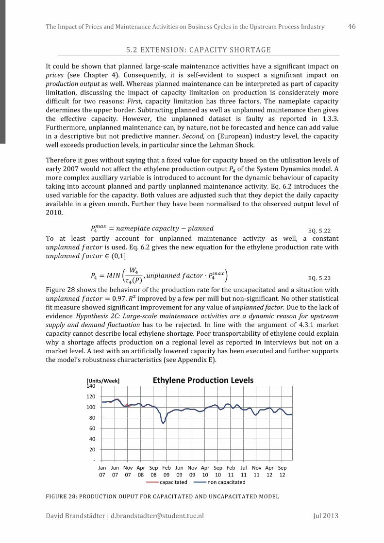
The Impact of Prices and Maintenance Activities on Business Cycles in the Upstream Process Industry 46
David Brandstädter | [email protected] Jul 2013
5.2 EXTENSION: CAPACITY SHORTAGE
It could be shown that planned large-scale maintenance activities have a significant impact on prices (see Chapter 4). Consequently, it is self-evident to suspect a significant impact on production output as well. Whereas planned maintenance can be interpreted as part of capacity limitation, discussing the impact of capacity limitation on production is considerately more difficult for two reasons: First, capacity limitation has three factors. The nameplate capacity determines the upper border. Subtracting planned as well as unplanned maintenance then gives the effective capacity. However, the unplanned dataset is faulty as reported in 1.3.3. Furthermore, unplanned maintenance can, by nature, not be forecasted and hence can add value in a descriptive but not predictive manner. Second, on (European) industry level, the capacity well exceeds production levels, in particular since the Lehman Shock.
Therefore it goes without saying that a fixed value for capacity based on the utilisation levels of early 2007 would not affect the ethylene production output 𝑃4 of the System Dynamics model. A more complex auxiliary variable is introduced to account for the dynamic behaviour of capacity taking into account planned and partly unplanned maintenance activity. Eq. 6.2 introduces the used variable for the capacity. Both values are adjusted such that they depict the daily capacity available in a given month. Further they have been normalised to the observed output level of 2010.
𝑃4𝑚𝑎𝑥 = 𝑛𝑎𝑚𝑒𝑝𝑙𝑎𝑡𝑒 𝑐𝑎𝑝𝑎𝑐𝑖𝑡𝑦 − 𝑝𝑙𝑎𝑛𝑛𝑒𝑑 EQ. 5.22 To at least partly account for unplanned maintenance activity as well, a constant 𝑢𝑛𝑝𝑙𝑎𝑛𝑛𝑒𝑑 𝑓𝑎𝑐𝑡𝑜𝑟 is used. Eq. 6.2 gives the new equation for the ethylene production rate with 𝑢𝑛𝑝𝑙𝑎𝑛𝑛𝑒𝑑 𝑓𝑎𝑐𝑡𝑜𝑟 ∈ (0,1]
𝑃4 = 𝑀𝐼𝑁 �𝑊4
𝜏4(𝑃) ,𝑢𝑛𝑝𝑙𝑎𝑛𝑛𝑒𝑑 𝑓𝑎𝑐𝑡𝑜𝑟 ∙ 𝑃4𝑚𝑎𝑥� EQ. 5.23
Figure 28 shows the behaviour of the production rate for the uncapacitated and a situation with 𝑢𝑛𝑝𝑙𝑎𝑛𝑛𝑒𝑑 𝑓𝑎𝑐𝑡𝑜𝑟 = 0.97. 𝑅² improved by a few per mill but non-significant. No other statistical fit measure showed significant improvement for any value of unplanned factor. Due to the lack of evidence Hypothesis 2C: Large-scale maintenance activities are a dynamic reason for upstream supply and demand fluctuation has to be rejected. In line with the argument of 4.3.1 market capacity cannot describe local ethylene shortage. Poor transportability of ethylene could explain why a shortage affects production on a regional level as reported in interviews but not on a market level. A test with an artificially lowered capacity has been executed and further supports the model’s robustness characteristics (see Appendix E).
FIGURE 28: PRODUCTION OUPUT FOR CAPACITATED AND UNCAPACITATED MODEL
-
20
40
60
80
100
120
140
Jan07
Jun07
Nov07
Apr08
Sep08
Feb09
Jun09
Nov09
Apr10
Sep10
Feb11
Jul11
Nov11
Apr12
Sep12
[Units/Week] Ethylene Production Levels
capacitated non capacitated

47 Basic Supply Chain model
Master Thesis TU/e Eindhoven
5.3 EXTENSION: IMPORTS
Evidently, trade and hence import of polyethylene products has increased over the last year and thus import of polyethylene products has increased over the last years as well (see 1.5.3). Managers report that polyethylene product flows to Europe gained importance and are considered in planning decisions. As the extent of imports differs between the three product groups in question, each is analysed individually. Figure 29 shows the relative growth with LLDPE imports increasing the most.
FIGURE 29: POLYETHYLENE IMPORT (EUROSTAT, 2013)
However, Table 13 shows that LLDPE imports only have a significant correlation with the polyethylene spreads. Correlations with production or sales are insignificant. A cross-correlation of imports and production over ± 6 months did not show any significant correlation either (see Figure D-4). Regarding the impact on prices, a cross-correlation between the total polyethylene imports and the polyethylene price spread unveiled a significant correlation for the +1 lead indicating that this month’s import figures have an influence on next month’s price spread. Nonetheless, adding imports to the Maintenance-Price Model introduced in Chapter 4 does not add significant value (see Table D-3). This suggests that oil price already explains the accounted variance. Consequently, due to the lack of statistical evidence, Hypothesis 2D: Imports of polyethylene to Europe influence local production output has to be rejected.
CORRELATION WITH LLDPE IMPORTS
PEARSON COEFF.
SIG. (2-TAILED)
LLDPE Imports 1.000
LLDPE Price .346** .003
LLDPE Production -.055 .648
LLDPE Sales .087 .466
bold italic: Correlation is significant at the 0.01 level (2-tailed).
TABLE 13: CORRELATION OF IMPORTS AND PRODUCTION
A correlation test between imports and stock was significant for all three polymers. Interestingly is the direction of the correlation. HDPE and LDPE show negative correlation, only LLDPE a positive one (see Table D-4). However, due to the fact that also (lagged) production is significantly correlated with stock levels, it cannot be ruled out that this is caused by general market movements and hence also exports show significant correlation. An additional explanation could be that demand increase is to a large extent compensated by imports. The latter two could not be tested due to lack of reliable data.
0%
50%
100%
150%
200%
Jan 07 Jan 08 Jan 09 Jan 10 Jan 11 Jan 12
PE Import (2010 = 100%)
HDPE Import LLDPE Import LDPE Import

The Impact of Prices and Maintenance Activities on Business Cycles in the Upstream Process Industry 48
David Brandstädter | [email protected] Jul 2013
6 ADVANCED SUPPLY CHAIN MODEL
The supply chain model introduced in 5.1 accurately describes the behaviour of the plastics supply chain. However, since the Lehman Wave, noise has increased. Part of this noise is due to the impact of price both on feedstock purchase and on polyethylene buying decisions (see 5.1.4). This chapter introduces a price effect on the buying behaviour of converters following Corbijn (2013). In addition, an effect of price on the feedstock purchase of Echelon 4 is introduced. 6.1 investigates the matter of calibration, 6.2 discusses the model fit.
The reasoning behind the price extension is that observed price has an influence on the desired stock level and by that eventually on order size. The desired stock level is extended by a stock effect as in Eq. 6.1. The stock effect is the derivative of the price times an adjusting stock effect ASE (see Eq. 6.2). Stock effects are introduced for all converter echelon 𝑛 = 2.1, 2.2, 2.3 and the cracker echelon 𝑛 = 4. Prices are absolute, non-normalised values. For the converter echelons, the polyethylene price is used. Following 5.1.4, the cracker echelon reacts on the naphtha price. To best capture the monthly price settling of the polyethylene contract price, converter echelons reply to the price derivative over 5 weeks. Naphtha is a spot price, thus the derivative over 1 week is used. Figure 30 shows exemplary how the extension is implemented in the Vensim model.
𝑆𝑛� = 𝐹𝑛 ∙ 𝐶𝑛� ∙ (1 + 𝑠𝑡𝑜𝑐𝑘 𝑒𝑓𝑓𝑒𝑐𝑡𝑛) EQ. 6.1
𝑠𝑡𝑜𝑐𝑘 𝑒𝑓𝑓𝑒𝑐𝑡𝑛 = 𝑃𝑟𝑖𝑐𝑒 �𝑑𝑑𝑡� ∙ 𝐴𝑆𝐸𝑛 EQ. 6.2
FIGURE 30: STOCK EFFECT IN VENSIM MODEL (M2)
6.1 PARAMETER ESTIMATION
The price extension focuses on the second, post-Lehman Shock period starting January 2009. Two major events characterise the beginning of this second period: First, ethylene prices are no longer settled quarterly but monthly (see 4.1.2). Second, the industry is still recovering from the most severe demand and price shock of the decade (see 1.1.1 and 1.4.2). Coinciding with these events is the regular spring turnaround season. From a System Dynamics modelling point of view, these effects pose a challenge as “stocks give systems inertia and provide them with memory” (Sterman, 2000, p. 192). The system of the previous chapter reacted the way it did because of its state prior to the Lehman Wave. Taking into account the immense delay effects of the model, the “memory reach” is at least one year long (see 5.1.2). Hence, the starting point for calibration of the one-echelon model is expected to be highly relevant and the following hypothesis is stated:
4 ForecastCHEMICALS 4 change in exp
C2 order
4 Desired C2stock
4 Desired C2inventory coverage
4 C2 forecastadjustment time
-
+
4 Adjustment C2stock ++
4 C2 stockadjustment time
-
4 FeedstockOrders
4 desired WIP C2stock
+
+
of
+
<4 C2 productiontime>
<3 C2 orders>
4 Stock Effect+
4 ASE
+
<Naphtha dt [ex]>+

49 Advanced Supply Chain Model
Master Thesis TU/e Eindhoven
HYPOTHESIS 3A: STARTING THE CALIBRATION IN AN UNSTABLE PERIOD BIASES THE MODEL FIT DISTINCTIVELY.
To investigate this claim the model is calibrated with the same initial values and bounds as the Model1A (see 5.1). Five different starting points for the calibration are selected reaching from the first week in 2009 to mid-July, well after the turnaround season (see Table 14). The stock effect is not yet included in the model and hence all 𝐴𝑆𝐸𝑛 = 0.
WEEK DATE (APPROX.) 𝑡1 = 106 01/01/2009 𝑡2 = 113 22/02/2009 𝑡3 = 120 08/04/2009 𝑡4 = 127 01/06/2009 𝑡5 = 134 15/07/2009
TABLE 14: DIFFERENT STARTING POINTS FOR MODEL M2A
Figure 31 shows the calibrated model outcomes. It can be observed that all five models show systematic bias and overestimate the production volume. Even the best fit, 𝑡5, only has a few data points where modelled values are below that of observed ones.
FIGURE 31: ETHYLENE PRODUCTION FOR DIFFERENT CALIBRATION STARTING POINTS (M2A)
Table 15 shows the related fit measures confirming the observation of significant bias (high 𝑈𝑀-values). The decreasing payoff value supports Hypothesis 3A: 𝑡1 is closest to the disrupting effects of Lehman Wave and price settlement change. 𝑡5 with most distance to those effects has the best payoff-value. However, the fit is significantly worse. In contrast, the calibration beginning in 2007 (see 5.1.1) has a payoff value of -4074 over the entire period. Hence, Hypothesis 3A: Starting the calibration in an unstable period biases the model fit distinctively, can be confirmed.
80
85
90
95
100
105
110
115
Jan 09 Jul 09 Jan 10 Jul 10 Jan 11 Jul 11 Jan 12 Jul 12
[units/week] Modelled and observed ethylene production (M2A)
t1 = 106
t2 = 113
t3 = 120
t4 = 127
t5 = 134
observed

The Impact of Prices and Maintenance Activities on Business Cycles in the Upstream Process Industry 50
David Brandstädter | [email protected] Jul 2013
NAME 𝒕𝟏 𝒕𝟐 𝒕𝟑 𝒕𝟒 𝒕𝟓 Payoff-Value -7880 -6343 -6015 -5652 -4850
𝑅² 0.272 0.445 0.470 0.474 0.553 𝑈𝑀 0.265 0.446 0.456 0.430 0.444 𝑈𝑆 0.117 0.062 0.127 0.066 0.038 𝑈𝐶 0.618 0.492 0.417 0.504 0.518
TABLE 15: STATISTICS OF DIFFERENT CALIBRATION STARTING POINTS (MODEL M2A)
A biased model fit is usually mitigated by parameter adjustment (Sterman, 2000, p. 876). Nonetheless, a change of the tolerance band for parameters cannot be justified as it was not reported in any of the expert interviews (see 1.6.2). Consequently the model has been recalibrated over the full time period (starting in 2007) using the initial parameter values and tolerance bands (see 5.1.1). Model fit is reported in 6.2.
The stock effect is a measure of how sensitive stocks are adjusted to price movements. Statements of the expert interviews that price sensitivity has increased recently and the confirmed Hypothesis 2B lead to the expectations that stock effects are larger in the post-Lehman period than before. Hence the following hypothesis is stated:
HYPOTHESIS 3B: STOCK EFFECTS ARE LARGER IN THE POST-LEHMAN PERIOD THAN BEFORE.
T the four 𝐴𝑆𝐸 parameters have been estimated for the full horizon, for the entire post-Lehman period starting in 2009 (𝑡1 = 106 𝑤𝑒𝑒𝑘𝑠) and from the time when the system is relatively stable (𝑡5 = 134 𝑤𝑒𝑒𝑘𝑠).
FULL HORIZON (5 WEEKS)
POST-LEHMAN WAVE (106 WEEKS)
SHORTENED SECOND PERIOD (134 WEEKS)
𝐴𝑆𝐸4 -2.833 -3.0323 -3.150 𝐴𝑆𝐸2.1 0.189 -0.036 0.005 𝐴𝑆𝐸2.2 -0.993 -1.229 -1.692 𝐴𝑆𝐸2.3 0.969 1.197 1.340
TABLE 16: STOCK EFFECTS FOR DIFFERENT PERIODS
Table 16 lists the development of the effect over the three periods. Four observations can be made. First, no effect changes the direction of the periods. All parameters grow absolutely with the exception of 𝐴𝑆𝐸2.1 which remains close to zero. This indicates coherent model behaviour over all parameters. Second, the effect for naphtha (𝐴𝑆𝐸4) and LDPE purchases (𝐴𝑆𝐸2.2) is negative indicating that a price increase leads to reduced orders. 𝑇ℎ𝑖𝑟𝑑, HDPE purchases (𝐴𝑆𝐸2.1) do not react on prices. In absolute terms an 𝐴𝑆𝐸 of 0.189 means that a price increase of 10% leads to an inventory coverage increase of 1.89%. Fourth, LLDPE purchases (𝐴𝑆𝐸2.3) are positively influenced by price movements. A price increase leads to increased orders.
It can be concluded that not only converters but also the upstream is increasingly reacting to price. Further, there seems to be a clear distinction between product types whether and how orders are influenced by price changes. Unfortunately, due to lack of experts from the converter echelon, the figures cannot be verified but they pose an interesting addition to the findings of Corbijn (2013) who quantified certain price anticipation effects. Possible explanations could be the different price level of different grades as well as production techniques and hence, in

51 Advanced Supply Chain Model
Master Thesis TU/e Eindhoven
combination with volume, different stock holding risks. Because the HDPE parameter is the only one not showing an increase in absolute value, Hypothesis 3B: Stock effects are larger in the post-Lehman period than before, is accepted.
6.2 MODEL FIT/ADDED VALUE
Following the findings of the previous section, a stock effect will only be introduced at week 134 once the system is in a relatively stable environment. The overall fit increased slightly to an 𝑅²-value of .830, a plus of 2% (for other fit measures, see Table D-5: Behaviour reproduction statistics for Model M2A).
METRIC M1A (NO PRICE EFFECT) M2A (PRICE EFFECT) 𝑅² 0.651 0.677
𝑀𝐴𝐸 2.85 2.82
𝑀𝐴𝑃𝐸 2.99% 2.96%
𝑀𝐴𝐸/𝑀𝐸𝐴𝑁 2.99% 2.95%
𝑅𝑀𝑆𝐸 3.66 3.52
𝑈𝑀 0.001 0.000
𝑈𝑆 0.022 0.017
𝑈𝐶 0.978 0.983
TABLE 17: COMPARISON OF MODEL M1A AND M2A IN POST-LEHMAN WAVE PERIOD
Table 17 shows the comparison of the relevant second period. However, although stock effects increase (see 6.1), the increase in statistical fit is minor. A two-tailed dependent t-test between the squared point-by-point errors of the two different models was non-significant (𝑡(208) =1.857,𝑝 < .1, 𝑟 = .13).
FIGURE 32: COMPARISON OF M1A AND M2A MODEL FIT
The model output of M1A (no price) and M2A (price effect) are plotted in Figure 32. Due to the insignificant change in model fit, a forecast feature for the advanced supply chain model (M2A) is not implemented.
60
70
80
90
100
110
120
Jan 09 Jul 09 Jan 10 Jul 10 Jan 11 Jul 11 Jan 12 Jul 12
[units/week] Comparison of modelled ethylene output
M2A
observed
M1A

The Impact of Prices and Maintenance Activities on Business Cycles in the Upstream Process Industry 52
David Brandstädter | [email protected] Jul 2013
7 MANAGERIAL INSIGHTS
In three subsections this chapter presents key insights of the study with practical relevance. Given advice is tailored for European ethylene producers but can be of interest for other stakeholders in the plastic value chain as well. Portability to other industries is limited due to the specific characteristics immanent to the petrochemical industry.
7.1 GENERAL INSIGHTS
The Lehman Shock in September 2008 divides the investigated time horizon from January 2005 to December 2012 in two halves: 2005 to 2008 and 2009 to 2012. Since 2009 cracker monthly utilisation rates seldom reached 90% whereas before they similarly seldom dropped below that figure. Despite the long-standing low level of demand, capacity has not been reduced. On the supply side, Europe’s structurally worse feedstock price situation has been intensified due to the rise of shale gas and oil cracking in the US Both led to eroding margins and negative trends of price spreads (see 1.4.2).
Next to the change in the somewhat exogenous factors a change in behaviour within the plastics supply chain could be detected coinciding with the beginning of the post-Lehman period. A significant impact of large-scale cracker maintenance activities and turnarounds could be observed since 2009 (see Table 2). Likewise, stock effects – the response of desired inventory levels on price movements – have increased over time (see Table 15). In addition, HDPE price volatility has frequently been above that of ethylene and naphtha (see Figure 9). With the exception of the stock effect, which was also observed on feedstock purchase, all mentioned particulars have in common that they are located at the interface of upstream and downstream echelons – namely polyethylene producers and converters.
7.2 INSIGHTS AND APPLICATION OF THE MAINTENANCE-PRICE MODEL
As mentioned above, a significant impact of planned maintenance activity could only be observed since 2009 with no significant effect in the years before the Lehman Shock. Precisely, only the contract price of ethylene reacts on planned maintenance, effects for spot prices are minor or insignificant. It could also be shown that converters do not stock-up before turnaround-season. This indicates that the origin of the price spread response on maintenance activities lies within the upstream, namely the ethylene and polyethylene producers. For turnaround planning, this means that timing is highly important and a schedule asynchronous to that of competitors profitable.
Because turnarounds are planned well in advance and extent as well as timing is known several months before the event, the found effect on price spreads can be used to forecast them. Figure 33 shows the forecasts’ error for a six month forecast solely based on data available in December 2012. The constants are derived from the Maintenance-Price regression model as discussed in 4.1.2. Next to the crude oil price of December 2012, only data for planned maintenance activities from an industry report released in December 2012 is used.

53 Managerial Insights
Master Thesis TU/e Eindhoven
FIGURE 33: ERROR OF PRICE SPREAD FORECASTS
Both forecasts show a high level of accuracy up to four months in the future. Because the naphtha price can be seen as exogenous to the plastic value chain (see 1.4) and reliable forecasts are available it can be combined with the forecasted spread in order to forecast the specific product price.
The application and implementation within current S&OP depends on the horizon of the forecast. In the industry, contract prices are settled one month in advance. Information over upcoming price development is a strong negotiation advantage. Many routing and transportation decisions, such as vessel and terminal planning have a time horizon of 1-2 months as well. The price forecast helps to determine expected profitability or required margin on such short-term contracts. Small-scale maintenance activities can usually be planned more flexibly – an accurate price forecast gives room to plan in such a way that losses are minimised. Furthermore, it helps in the decision whether to overproduce and store product to buffer the production outage. In general, accurate price spread forecasts support the cash flow and financial planning.
The model can easily be implemented in spread sheet software and requires, aside of a sporadic rerun of the regression analysis, little data maintenance.
7.3 INSIGHTS AND APPLICATION OF THE SUPPLY CHAIN MODEL
The System Dynamics model accurately describes ethylene production and polyethylene stock levels while being steered solely by end-market demand data. This is a relevant insight and should raise awareness towards the echelon closest to the end-market. Tied in with this fact is the model’s sensitivity towards changes in the end market. Minor demand shocks amplify throughout the chain and cause severe oscillation at the upstream. Whereas this is known in generic terms of the Bullwhip Effect, the model helps to quantify and anticipate these effects.
Among the most sensitive parameters from the upstream echelons are desired inventory coverage levels for ethylene and polyethylene producers. Decision makers have to be aware of the effect and manage inventories carefully. This is particularly interesting as both inventory stock levels and inventory coverage have increased in 2011 and 2012 close to the levels prior to
-0.7%
16.5% 5.5%
-0.4%
31.0% 16.9%
-4.4%
6.8% 5.6% 2.1%
24.5% 10.9%
-100%
-50%
0%
50%
100%
Dec 12 Jan 13 Feb 13 Mar 13 Apr 13 May 13 Jun 13
Price spread forecast error (forecasted in Dec 2012)
Ethylene spread
Polyethylene spread

The Impact of Prices and Maintenance Activities on Business Cycles in the Upstream Process Industry 54
David Brandstädter | [email protected] Jul 2013
the Lehman bankruptcy. This means that after a period of relatively tightly managed stocks in response to the synchronised destocking causing the Lehman Wave, stocks are increasing again.
Two extensions of the model were tested but did not show relevant effect: Capacity limitation and polyethylene imports. The model is based on aggregated industry data; hence it is still possible that capacity limitation, such as a cracker turnaround, has effects on production outputs on a regional and certainly a firm level. However, a statement derived directly from the model findings is that large maintenance activities have an effect on prices but not on production. This is, such limitations are only visible on a market level as an effect on price. Similarly, polyethylene imports influence prices but not production or sales volume. Here, a regional effect can likely be excluded leading to the conclusion that an analysis or forecast of import volumes should focus on price effects, not on volumes.
Stock effects, an adjustment of order size according to price movement, could be isolated. Naphtha orders decrease when price rises and vice versa. For polyethylene orders the picture is threefold: A stock effect for HDPE was not identified. LDPE orders show similar, negatively correlated behaviour (orders increase when price is falling). Contrary, LLDPE purchases have a positive relationship with product prices. An increase in product price leads to an increase in order size and vice versa. All effects were measured at different points in time and showed coherent absolute growth over the observed horizon (2007 to 2012). This indicates that the model correctly quantifies these effects. However, the difference in polarity cannot be explained at this point because of the relatively large variety of polymer grades and production techniques. It is advised to test the model with different prices to further analyse the effect on a product level.
The model fails to create an adequate fit when the starting point of calibration is set in the post-Lehman period. This indicates instability of the system. A System Dynamics model has a certain degree of memory expressed by stocks (this includes “mental” stocks like anchored forecast levels, material in transport, backlogs and work in process stocks). Because a model initialised well before the Lehman Wave shows good fit in the post-Lehman period as well, it can be concluded that any planning decision has to be seen in perspective to past measures and responses which may not yet been absorbed by the system.
Although the advanced supply chain model including price did not show a better model fit than the model without price, it cannot be concluded that price does not have an effect on volumes. It does mean, however, that a model based on volume alone can already explain a large amount of upstream supply chain behaviour. Hence price and volume should be taken into account equitably in sales or planning decisions.
The model is implemented in Vensim, a System Dynamics software package. Due to its complexity in handling and interpreting outcomes, in particular that of forecasts, the model requests a certain level of experience. Data maintenance includes update of end market demand data which requires interpolation. A recalibration needs considerable computation time which can be reduced by applying the discussed 3-stage heuristic (see 5.1.1).

55 Conclusion and Further Research
Master Thesis TU/e Eindhoven
8 CONCLUSION AND FURTHER RESEARCH
This last chapter summarises the key findings of the study, in particular the result of the hypothesis and answers to the two research questions. Limitations of the study are discussed as well. Recommendation for further research is given. Like used throughout the thesis, upstream describes the two highest echelons in scope, ethylene and polyethylene producers, downstream the converter, OEM and end market echelon.
8.1 CONCLUSION
This study contributes to research in four ways: First, it could be shown that large-scale planned maintenance activities such as cracker turnarounds explain up to 28% of the variance in the spread between final product price of the upstream and the inbound feedstock price. Second, the one-echelon System Dynamics model based on volume and triggered solely by end market demand data can accurately describe upstream ethylene production and polyethylene stock levels. By this, scope of further applications has been extended substantially and outcome data has been cross validated. Third, the influence of price on orders of both converters and feedstock purchases is substantial. A model not taking into account price is missing market oscillation. A volume forecast for the upstream process industry thus has to take into account price to be accurate. Fourth, maintenance activities do not directly influence business cycles in the process industry but affect prices which again have an influence and add substantial noise to natural demand meant for consumption.
8.1.1 HYPOTHESES
The outcomes of the hypotheses allow an assessment of initial motivation and expectation of this endeavour. Table 18 lists all eight including outcome and document reference.
HYPOTHESIS OUTCOME REF.
1A Maintenance activities of cracker units have a positive effect on prices spreads of commodity products.
accepted 4.1
1B Converters stock-up before a maintenance period in order to buffer against uncertainty.
rejected 4.2
2A A linked single echelon model triggered by end-market demand can accurately describe observed de-stocking effects in the plastics supply chain.
accepted 5.1.3
2B A model not taking into account price performs worse in the post-Lehman period than before.
accepted 5.1.4
2C Large-scale maintenance activities are a dynamic reason for upstream supply and demand fluctuation.
rejected 5.2
2D Imports of polyethylene to Europe influence local production output.
rejected 5.3
3A Starting the calibration in an unstable period biases the model fit distinctively.
accepted 6.1
3B Stock effects are larger in the post-Lehman period than before
accepted 6.1
TABLE 18: OVERVIEW OF HYPOTHESES
Although it was expected through expert interviews (see 1.6.2) that cracker turnarounds have an influence on prices, this effect had not been quantified nor was the extent of maintenance taking into account in price forecasts. By conducting a step-wise regression analysis and paying
The Impact of Prices and Maintenance Activities on Business Cycles in the Upstream Process Industry 56
David Brandstädter | [email protected] Jul 2013
close attention to inflating effects such as price seasonality, auto- and cross-correlation, it could be shown that planned maintenance has a significant positive effect on price spreads and Hypothesis 1A could be accepted.
The sheer size and impact of operations of a cracker turnaround led to the expectation that converters stock up before a turnaround season in order to buffer against upcoming uncertainty. Inventory levels in the post-Lehman period are biased by price fluctuations caused by maintenance activities. A natural experiment, comparing the levels to the pre-Lehman period where maintenance did not yet have an influence on prices, showed that no up-stocking took place indicating that price is the driving factor for partly observed stock-ups. Further evidence is needed to accept a negative hypothesis that converters do not stock up but the positively formulated Hypothesis 1B has to be rejected.
The System Dynamics linked single echelon model has been applied successfully to the process industry before (see 2.1). It indeed could be shown that it is an adequate model to also describe the upstream process industry market and due to close model fit and extensive testing, Hypothesis 2A could be accepted.
Based on the results of the maintenance-price model (see 4.1) and the observed increased price volatility (see 1.4.2) it was expected that the influence of price on production and material flow has increased since the Lehman Wave. A significantly worse fit of the model in this second period supports the claim and Hypothesis 2B was accepted.
Because of the enormous impact of cracker turnarounds on a firm’s operations it was expected to see impact of turnarounds in production or order behaviour. However, such an effect could not be observed, presumably due to the relatively high level of aggregation. Firm- or regional-level of data is necessary to further investigate on this premise. In the context of this study, however, Hypothesis 2C had to be rejected.
Through expert interviews it was expected that the increase of polyethylene imports influences European production output. Despite the evident consideration in medium-term planning discussions, no such effect could be observed and Hypothesis 2D was rejected. Explanations could be a simple overstating of the effect, compensation by increasing exports or that alone excess demand is satisfied by imports.
It could be shown that the starting point of the calibration has severe influence on the System Dynamics model due to the memory effects in its stocks and Hypothesis 3A was accepted. The one-echelon model was not able to accurately describe the second, post-Lehman Shock period accurately without being anchored in the first period. It is important to understand for future applications that the model needs a relatively stable initial environment before it is being exposed to flow shocks.
Increased price sensitivity from converters’ side since the Lehman Shock has been reported by experts. It could be shown that stock effects grew within the observed time horizon and were larger in the post-Lehman period. Hence Hypothesis 3B was accepted. An increased effect could also be observed for the purchase of naphtha. Furthermore, LLDPE showed a positive stock effect indicating that orders increase when price rises.
8.1.2 RESEARCH QUESTIONS
The two research questions were derived from the introductory chapter, the literature review and the problem statement (see 3.1). The first question tackles structural, long-term characteristics of the plastics supply chain, the second question focuses on short- and medium-term dynamics.

57 Conclusion and Further Research
Master Thesis TU/e Eindhoven
RESEARCH QUESTION 1:
What are the underlying structural reasons in petrochemical supply chains causing high fluctuations experienced at the demand side of upstream players and what is the nature of the caused effects?
Two main structural reasons have been identified: The linked single-echelon model can accurately describe the upstream production outcome and shows that the model is highly sensitive to changes in the downstream demand. As it is triggered by end-market demand, changes in the last echelon, closest to the end-markets, amplify throughout the chain causing oscillation in the upstream. In general the direction of these effects is positive, a demand decrease downstream causes a (more severe) dip upstream but a significant overshoot cannot be observed. Observed noise is not captured by the model indicating that short-term fluctuations are due to factors not captured by the model.
Changes in the upstream inventory coverage have strong effects on the supply chain behaviour as well and are, next to polyethylene cycle production time, the most sensitive observable factor of the upstream echelons. Behavioural factors of the upstream such as adjustment times do not show high influence on the supply chain.
Effects of polyethylene imports and capacity limitation on the production output could not be observed. For capacity limitation (due to maintenance) there is a confirmed mitigation effect on price. Imports coincide with price movements as well, though deeper analysis is needed to confirm and describe this effect. Large-scale maintenance activities and price movements comprise the studied dynamics which led to the second research question.
RESEARCH QUESTION 2:
How do underlying dynamics in petrochemical supply chains facilitate and amplify these observed fluctuations on demand and supply side?
A positive and significant effect of planned maintenance on price spreads between ethylene (respectively polyethylene) on naphtha could be isolated. Introducing an influence of price movement on order behaviour of both polyethylene purchase from converters and feedstock purchase of ethylene producers was different from zero. Still, distinctive deviations from the model which cannot be interpreted as noise indicate that either the influence of price is more complex than a linear first-order effect on price changes or that these deviations are due to factors outside of the thesis’ scope.
The study could show that price has an influence on orders and is also used to react to dynamic effects such as large-scale maintenance. However, a model not taking into account price can already accurately describe the upstream plastic supply chain and captures most of the trends. Hence price alone cannot be a proxy for demand but has to be seen in combination with volume.

The Impact of Prices and Maintenance Activities on Business Cycles in the Upstream Process Industry 58
David Brandstädter | [email protected] Jul 2013
8.1.3 LIMITATIONS
The conducted study is clearly limited geographically to the European petrochemical industry. Other regions differ structurally e.g. on the supply side by access to cheaper feedstock (Saudi Arabia, lately USA, see 1.1.2) or on the demand side by growing end-market demand (Asia).
A temporary limitation is present as well: In particular the second of the two observed periods shows a large gap between supply capacity and demand. Due to the high operating costs of production units, it is unlikely that such a situation can persist. Once supply is synchronised to demand, capacity limitations become more important. Especially the role of price has to be revaluated since monthly contract prices did not exist yet in situations of high utilisation rates.
The study is limited to the commodity product ethylene and polyethylene. Other cracker derivatives are subject to a pure push characteristic as their volumes are determined by that of ethylene (see 1.1). It is likely that those product streams and prices behave differently and findings are not transferable.
The largest limitation is access, timeliness and accuracy of data. In particular the forecast quality highly depends on these factors. During the study endeavour it was observed that public data is often published too late and old data series are, sometimes significantly, corrected retroactively.
The used cubic spline interpolation captures the time series data well. However, it is not able to fully capture intra-month behaviour. This is a limitation since most described prices are settled in a monthly interval but in different times of the month. Further, reactions on short-term dynamics like small maintenance activities can have selective effects not visible in monthly data.
8.2 FURTHER RESEARCH
This section describes suggestions for further research beyond the abovementioned limitations.
Within the upstream process industry local or regional effects of capacity limitations can unveil dynamics not visible on aggregated industry level. Next to the mentioned cracker by-products, technology is in development to produce those products directly from dedicated input. Once it is economical to produce e.g. butadiene directly from butane instead of common cracker feedstock, this is likely to change the character of the petrochemical industry. The role of increasing imports and trade could make an interesting subject for a macro economical study.
A key subject to understand supply chain dynamics in the plastics supply chain is the interface of upstream (ethylene and polyethylene producers) and downstream (converters and OEMs). Both groups have fundamentally different business and production characteristics (see Table H-1). The polyethylene prices work as pivot between both parties. In addition, inventory effects, in particular the perceived inventory fill rate and price anticipation are expected to play an important role in observed dynamics. See Appendix H for a brief discussion on this topic.
Related but not limited to this topic is a price finding model for the commodity industry. Current System Dynamics models are often related to reference demand or price and focus on emphasize the role of long-term capacity. This study alone identified two factors influencing the price settlement, namely maintenance activity and price movement. A sensitive additional topic is the one of horizontal collaboration in the upstream process industry and the potential benefits in efficiency increase. At last, the field of seasonal capacity is hardly reviewed in current literature.

i List of Abbreviations
Master Thesis TU/e Eindhoven
9 LIST OF ABBREVIATIONS
APPE Association of Petrochemicals Producers in Europe.
ARG ARG mbh & Co. KG.
ASE Adjusting stock effect.
bln Billion.
C2 Ethylene.
CIF Cost, Insurance, Freight.
CMAI Chemical Market Associates Inc..
CP Contract Price.
DINALOG Dutch Institute for Advanced Logistics.
DSM Dutch State Mines, former De Nederlandse Staatsmijnen.
EU European Union.
FOB Free on Board.
FTE Full-time equivalent.
GDP Gross domestic product.
HDPE High density polyethylene.
HIS IHS Inc.
IQPC International Quality & Productivity Center.
ITEM Innovation, Technology, Entrepreneurship & Marketing.
LDPE Low density polyethylene.
LLDPE Low linear density polyethylene.
MAE Mean absolute error.
MAPE Mean absolute percent error.
NAFTA North American Free Trade Agreement.
OEM Original equipment manufacturer.
OPAC Operations, Planning, Accounting and Control.
OPEC Organization of the Petroleum Exporting Countries.
POLYETHYLENE Polyethylene.
PMRC Petrochemicals Market Research Committee.
PP Polypropylene.
RMSE Root mean square error.
S&OP Sales and operations planning.
SABIC Saudi Basic Industries Corporation.
SBU Strategic Business Unit.
SC Supply Chain.
SCM Supply Chain Management.
UK United Kingdom.
US United States (of America).
WIP Work in process.
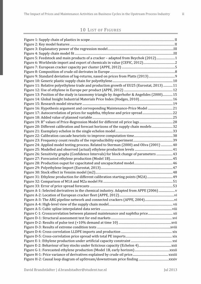
The Impact of Prices and Maintenance Activities on Business Cycles in the Upstream Process Industry ii
David Brandstädter | [email protected] Jul 2013
10 LIST OF FIGURES
Figure 1: Supply chain of plastics in scope ............................................................................................................. II Figure 2: Key model features ....................................................................................................................................... II Figure 3: Explanatory power of the regression model ..................................................................................... III Figure 4: Supply chain model fit ................................................................................................................................ III Figure 5: Feedstock and main products of a cracker – adapted from Beychok (2012) ........................ 1 Figure 6: Worldwide import and export of chemicals in value (CEFIC, 2012) ......................................... 2 Figure 7: European cracker capacity per cluster (APPE, 2012) ..................................................................... 5 Figure 8: Composition of crude oil derivates in Europe .................................................................................... 8 Figure 9: Standard deviation of log-returns, nased on prices from Platts (2013) .................................. 9 Figure 10: Generic plastic supply chain for polyethylene .............................................................................. 10 Figure 11: Relative polyethylene trade and production growth of EU25 (Eurostat, 2013) ............ 11 Figure 12: Use of ethylene in Europe per product (APPE, 2012) ............................................................... 12 Figure 13: Position of the study in taxonomy triangle by Angerhofer & Angelides (2000) ............. 15 Figure 14: Global Insight Industrial Materials Price Index (Hodges, 2010) ........................................... 16 Figure 15: Research model structure ..................................................................................................................... 19 Figure 16: Hypothesis argument and corresponding Maintenance-Price Model ................................ 21 Figure 17: Autocorrelation of prices for naphtha, tthylene and price spread ....................................... 22 Figure 18: Added value of planned variable ........................................................................................................ 25 Figure 19: R² values of Price-Regression Model for different oil price lags ........................................... 28 Figure 20: Different calibration and forecast horizons of the supply chain models ........................... 32 Figure 21: Exemplary echelon in the single echelon model .......................................................................... 33 Figure 22: Calibration cascade heuristic to improve computation time .................................................. 38 Figure 23: Frequency count results of the reproducibility experiment ................................................... 39 Figure 24: Applied model testing process. Related to Sterman (2000) and Oliva (2001) ............... 40 Figure 25: Modelled and observed (actual) ethylene production levels ................................................. 41 Figure 26: Sensitivity graphs (Confidence Intervals) for block change of parameters ..................... 43 Figure 27: Forecasted ethylene production (Model 1B)................................................................................. 45 Figure 28: Production ouput for capacitated and uncapacitated model.................................................. 46 Figure 29: Polyethylene Import (Eurostat, 2013) ............................................................................................. 47 Figure 30: Stock effect in Vensim model (m2) .................................................................................................... 48 Figure 31: Ethylene production for different calibration starting points (M2A) ................................. 49 Figure 32: Comparison of M1A and M2a model Fit .......................................................................................... 51 Figure 33: Error of price spread forecasts ........................................................................................................... 53 Figure A-1: Selected derivatives in the chemical industry. Adapted from APPE (2006) ..................... v Figure A-2: Location of European cracker fleet (APPE, 2012) ....................................................................... vi Figure A-3: The ARG pipeline network and connected crackers (APPE, 2004) ...................................... vi Figure A-4: High-level view of the supply chain model ................................................................................... vii Figure A-5: Cubic spline interpolated data series ............................................................................................ viii Figure C-1: Crosscorrelation between planned maintenance and naphtha price ................................ xii Figure D-1: Structural assessment test for end markets ............................................................................... xvi Figure D-2: Results of pulse test (+10% demand at time 10) .................................................................... xvii Figure D-3: Results of extreme condition tests ............................................................................................... xviii Figure D-4: Cross-correlation LLDPE imports and production .................................................................. xix Figure D-5: Cross-correlation price spread with total PE imports ............................................................ xix Figure E-1: Ethylene production under artificial capacity constraint ..................................................... xxi Figure E-2: Behaviour of key stocks under ficticious capacity (Echelon 4) .......................................... xxii Figure G-1: Forecasted ethylene production (Model 1B, early horizon) ............................................. xxxii Figure H-1: Price variance of derivatives explained by crude oil price .............................................. xxxiii Figure H-2: Causal loop diagram of upStream/downstream price finding ....................................... xxxiv

iii List of Tables
Master Thesis TU/e Eindhoven
11 LIST OF TABLES
Table 1: Overview of used data sources ................................................................................................................ 13 Table 2: Correlation of planned maintenance activities on prices. ............................................................ 23 Table 3: Stepwise regression analysis on dependent price spreads ......................................................... 26 Table 4: 3-Step regression model for different oil price lags........................................................................ 27 Table 5: Definition of model parameters .............................................................................................................. 34 Table 6: Overview of observable parameters ..................................................................................................... 37 Table 7: Overview of behavioural parameters ................................................................................................... 37 Table 8: Different values for desired inventory coverage of Echelon 3 ................................................... 40 Table 9: Behaviour reproduction tests M1A. Adapted from Sterman (2000, p. 875) ........................ 42 Table 10: Statistical fit, partial model estimation – Echelon 3 ..................................................................... 42 Table 11: Comparison of basic model fit for different periods .................................................................... 44 Table 12: Calibration/forecast transition values for Model M1B ............................................................... 45 Table 13: Correlation of imports and production ............................................................................................. 47 Table 14: Different starting points for Model M2A ........................................................................................... 49 Table 15: Statistics of different calibration starting points (Model M2A) ............................................... 50 Table 16: Stock effects for different periods ........................................................................................................ 50 Table 17: Comparison of Model M1A and M2A in post-Lehman Wave period ..................................... 51 Table 18: Overview of hypotheses ........................................................................................................................... 55 Table B-1: List of interviewees in chronological order ..................................................................................... ix Table B-2: License plate capacity of installed European crackers (APPE, 2012) .................................... x Table C-1: Correlation of maintenance activities and prices (respectively price spreads)................ xi Table C-2: Correlation of monthly average prices of intermediate products (2009-12) .................. xii Table C-3: Correlation of polyethylene prices ................................................................................................... xiii Table C-4: Regression coefficients - maintenance price model .................................................................. xiv Table C-5: Swapped order in the ethylene regression model ..................................................................... xiv Table C-6: Regression coefficients crude oil lag -1 ............................................................................................. xv Table C-7: Regression models on oil price............................................................................................................. xv Table D-1: T-Tests for inventory coverage .......................................................................................................... xvi Table D-2: Correlations of different polyethylene import volumes on price spread ....................... xviii Table D-3: Regression model including polyethylene imports ................................................................... xix Table D-4: Correlation of imports and stocks ...................................................................................................... xx Table D-5: Behaviour reproduction statistics for Model M2A ...................................................................... xx Table F-1: Observable parameters of the basic supply chain model ...................................................... xxiii Table F-2: Behavioural parameters of the basic supply chain model .................................................... xxiv Table F-3: Overview of product split parameters ........................................................................................... xxv Table F-4: Theta split values .................................................................................................................................... xxv Table F-5: Confidence interval of parameters ................................................................................................. xxvii Table F-6: Most sensitive parameters of Model M1A ................................................................................. xxviii Table F-7: Parameter values and frequencies for 10 runs (Model M1A) ............................................. xxxi Table H-1: Categorisation of up- and downstream part of the supply chain ................................... xxxiii

The Impact of Prices and Maintenance Activities on Business Cycles in the Upstream Process Industry iv
David Brandstädter | [email protected] Jul 2013
12 APPENDICES

v Appendices
Master Thesis TU/e Eindhoven
Appendix A SUPPLEMENTARY FIGURES
FIGURE A-1: SELECTED DERIVATIVES IN THE CHEMICAL INDUSTRY. ADAPTED FROM APPE (2006)

The Impact of Prices and Maintenance Activities on Business Cycles in the Upstream Process Industry vi
David Brandstädter | [email protected] Jul 2013
FIGURE A-2: LOCATION OF EUROPEAN CRACKER FLEET (APPE, 2012)
FIGURE A-3: THE ARG PIPELINE NETWORK AND CONNECTED CRACKERS (APPE, 2004)

vii Appendices
Master Thesis TU/e Eindhoven
Rigid Packing
Building & Construction
Flex Packing
Industrial Film
Flex Packing
Industrial Film
4 CrackerFeedstock C2
HDPE
1.1.1 OEM A
0.1.1Consumer
Food
LDPE
LLDP
E
3 Polymers
C2: EthylenePE: PolyethyleneHDPE: High Density PolyethyleneLDPE: Low Density PolyethyleneLLDPE: Linear Low Density Polyethylene
PE import
1.1.2 OEM
1.1.3Industrial
0.1.2Consumer Non-Food
A
1.1.4 OEM
1.1.5Civil
Engineering works
0.1.4BuildingsA
1.2.1 OEM
1.2.2 OEM
1.2.3Agricultural
1.2.4Geo-
membrane
0.2.1Consumer
FoodB
B0.2.2
Consumer Non-Food
1.2.5Industrial
1.3.1 OEM
1.3.2 OEM
1.3.3Agricultural
1.3.4Geo-
membrane
0.3.1Consumer
FoodB
B0.3.2
Consumer Non-Food
1.3.5Industrial
2.1 HDPE Converter
2.2 LDPE Converter
2.3 LLDPE Converter
Eurostat: Retail sales of food, beverages and tobacco (G47 FOOD)
Eurostat: Retail sales of non-food products, except fuel (G47 NFOOD X G473)
Eurostat: Building permits – m² of useful floor area (Euro area)
Eurostat: Retail sales of food, beverages and tobacco (G47 FOOD)
Eurostat: Retail sales of non-food products, except fuel (G47 NFOOD X G473)
Eurostat: Retail sales of non-food products, except fuel (G47 NFOOD X G473)
Eurostat: Retail sales of food, beverages and tobacco (G47 FOOD)
Eurostat: Manufacture of food products (C10)
Eurostat: Production Index Capital Goods (MIG CAG)
Eurostat: Production Index Intermediate & Capital Goods (MIG ING
CAG)
Eurostat: Manufacture of food products (C10)
Eurostat: Production Index Capital Goods (MIG CAG)
Eurostat: Production Index Intermediate & Capital Goods (MIG ING
CAG)
Eurostat: Manufacture of food products (C10)
Eurostat: Production Index Consumer Goods except food (MIG COG X Food)
Eurostat: Production Index Consumer Goods except food (MIG COG X Food)
Eurostat:Manufacture of food products and beverages (C10, C11)
Eurostat: Production Index Intermediate & Capital Goods (MIG ING CAG)
Eurostat: Production Index Civil Engineering Works (F CC2)
Eurostat: Production Index Buildings (F CC1)
Eurostat: Production Index Consumer Goods except food (MIG COG X Food)
Eurostat:Manufacture of food products and beverages (C10, C11)Industry report
Industry report
SABIC operated
Customer (tier 1+2)
Customer (tier >2)
Product
End market
FIGURE A-4: HIGH-LEVEL VIEW OF THE SUPPLY CHAIN MODEL

The Impact of Prices and Maintenance Activities on Business Cycles in the Upstream Process Industry viii
David Brandstädter | [email protected] Jul 2013
FIGURE A-5: CUBIC SPLINE INTERPOLATED DATA SERIES
0
20
40
60
80
100
120
140
2007
2007
2007
2007
2007
2008
2008
2008
2008
2008
2009
2009
2009
2009
2009
2010
2010
2010
2010
2011
2011
2011
2011
2011
2012
2012
2012
2012
2012
[Units/week] Interpolated ethylene production data
Original values Interpolated

ix Appendices
Master Thesis TU/e Eindhoven
Appendix B BACKGROUND INFORMATION
NAME POSITION DEPARTMENT BUSINESS (UNIT) Person 1 Full Professor OPAC TU/e Eindhoven Person 2 PhD student OPAC TU/e Eindhoven Person 3 Project Manager SC Improvements SABIC Chemicals Person 4 Manager Demand Planning SC Planning SABIC Chemicals Person 5 Supply & Inventory Manager SC Planning SABIC Chemicals Person 6 Supply & Inventory Manager SC Planning SABIC Chemicals Person 7 Manager Supply Chain
Planning & Optimisation SC Planning SABIC Chemicals
Person 8 Sales Manager Heavy By-Products
Aromatics SABIC Chemicals
Person 9 Sales Manager Propylene Olefins & Intermediates
SABIC Chemicals
Person 10 Master Production Scheduler SC Management SABIC Chemicals Person 11 Planning Optimization
Analyst SC Planning SABIC Chemicals
Person 12 Market Intelligence Business Strategy SABIC Chemicals Person 13 Business Controller SCM Business Strategy SABIC Chemicals Person 14 Manager Supply Chain
Improvements SC Improvements SABIC Chemicals
Person 15 Engineer Supply Chain Improvements
SC Improvements SABIC Chemicals
Person 16 Manager Sourcing & Contracting
SC Management SABIC Chemicals
Person 17 Planner & Scheduler Business Olefins Turnarounds
SABIC Chemicals
Person 18 Market Intelligence Business Strategy SABIC Polymers Person 19 Manager SC Planning
Polyolefins O&G Europe SABIC Chemicals
Person 20 Business Manager Olefins O&G Europe SABIC Chemicals Person 21 Controller Business Strategy SABIC Polymers Person 22 Demand Manager PE SC Planning SABIC Polymers Person 23 Business Manager C4s Aromatics &
Oxygenates SABIC Chemicals
Person 24 Assistant Professor ITEM TU/e Eindhoven Person 25 Director SC Chemicals Europe SC Europe Chemicals SABIC Chemicals Person 26 Manager Technical Marketing
PP Technical Marketing SABIC Polymers
Person 27 Business Development Manager
HDPE SABIC Polymers
Person 28 Manager Technical Marketing LD/LLDPE
SABIC Polymers
Person 29 Market Intelligence Business Strategy SABIC Chemicals Person 30 Project Manager Supply Chain
Improvements SABIC Chemicals
Person 31 International Account Manager
Sales SABIC Polymers
Person 32 Product Sales Manager Sales SABIC Polymers Person 33 Market Intelligence Officer Business Strategy SABIC Chemicals
TABLE B-1: LIST OF INTERVIEWEES IN CHRONOLOGICAL ORDER

The Impact of Prices and Maintenance Activities on Business Cycles in the Upstream Process Industry x
David Brandstädter | [email protected] Jul 2013
OPERATOR LOCATION REGION CAPACITY ETHYLENE 2011 [KT/YEAR]
AUSTRIA Schwechat OMV E 500
BELGIUM BASF Antwerp NW 1080 FAO Antwerp No.1 NW 230 FAO Antwerp No.2 NW 570 FAO Antwerp No.3 NW 580
FINLAND Borealis Porvoo N 380
FRANCE AP Feyzin Feyzin S 240 Total Carling No.1 NW 340 Total Gonfreville NW 520 Polimeri Europa Drunkerque NW 380 ExxonMobil N.D.G. NW 400 LyondellBasell Berre NW 460 Naphtachimie Lavera S 740
GERMANY BASF Ludwigshafen No.1 NW 240 BASF Ludwigshafen No.2 NW 420 Dow Böhlen E 510 Heide Refinery Heide NW 108 Shell Wesseling 2A NW 260 LyondellBasell Wesseling G4 NW 260 LyondellBasell Wesseling G6 NW 760 Ineos Dormagen No.4 NW 530 Ineos Dormagen No.5 NW 670 OMV Burghausen NW 445 Ruehr Oel Gelsenkirchen No.3 NW 540 Ruehr Oel Gelsenkirchen No.4 NW 540 LyondellBasell Muenchmuenster NW 400
ITALY Versalis Porto Marghera S 490 Versalis Priolo S 745 Versalis Brindisi S 440 Polimeri Europa Brindisi S 440
THE NETHERLANDS Dow Terneuzen No.1 NW 535 Dow Terneuzen No.2 NW 590 Dow Terneuzen No.3 NW 660 Sabic Europe Geleen No.3 NW 575 Sabic Europe Geleen No.4 NW 675 Shell Moerdijk NW 940
Norway Noretyl Rafnes N 575
Portugal Repsol Sines S 410
Spain Dow Tarragona S 670 Repsol Puertollano S 250 Repsol Tarragona S 702
Sweden Borealis Stenungsund N 610 Ineos Grangemouth G4
UNITED KINGDOM Ineos Grangemouth G4 UK 330 Ineos Grangemouth KG UK 730 ExxonMobil/Shell Mossmoran UK 830 Sabic Europe Wilton UK 865
OTHERS 40 TOTAL 23,765
1 FAO: 100% TOTAL 2 Borealis: 64% IPIC, 36% OMV 3 AP Feyzin: 57.5% TOTAL - 42.5% Solvay 4 Naphtachimie: 50% INEOS- 50% TOTAL
TABLE B-2: LICENSE PLATE CAPACITY OF INSTALLED EUROPEAN CRACKERS (APPE, 2012)

xi Appendices
Master Thesis TU/e Eindhoven
Appendix C REGRESSION RESULTS AND TESTS
PRODUCT PRICES/ PRICE SPREADS
unplanned planned all maintenance 2005-2012
before 2009
after 2009
2005-2012
before 2009
after 2009
2005- 2012
before 2009
after 2009
Naphtha - CIF NW Europe / Basis ARA [€]
PCC -.148 -.106 -.212 .005 -.026 .194 -.105 -.095 -.019 Sig. .076 .236 .074 .482 .430 .094 .155 .260 .450
Propane - CIF NW Europe [€/t]
PCC -.091 -.175 -.056 -.046 -.021 .080 -.104 -.139 .018 Sig. .188 .117 .353 .330 .443 .295 .156 .173 .451
Ethylene - Delivered W. Europe [CONTRACT]
PCC .133 ,340** -,242* ,327** ,258* ,493** ,363** ,446** .198 Sig. .098 .009 .049 .001 .038 .000 .000 .001 .089
Ethylene - Delivered Ex ARG [SPOT, €/t]
PCC .021 .105 -.107 ,329** ,285* ,302* ,282** ,304* .155 Sig. .420 .239 .234 .001 .025 .018 .003 .018 .147
Ethylene - CIF NW Europe [SPOT €/t]
PCC -.016 -.015 -.039 ,260** .187 ,250* ,199* .141 .169 Sig. .438 .459 .395 .005 .102 .043 .026 .170 .126
Propylene Contained Value – Del. W. Eur. [CONTRACT, €/t]
PCC .089 ,315* -.144 ,323** ,254* ,416** ,327** ,425** .216 Sig. .194 .015 .164 .001 .041 .002 .001 .001 .070
Propylene Polymer Grade – Del. Germany [SPOT €/t]
PCC .012 -.109 .122 ,297** ,308* ,242* ,250** .173 ,294* Sig. .453 .230 .205 .002 .017 .049 .007 .119 .021
Propylene Polymer Grade - CIF NW Europe [SPOT, €/t]
PCC .012 -.106 .120 ,301** ,316* ,243* ,253** .182 ,293* Sig. .454 .236 .209 .001 .014 .048 .006 .108 .022
Benzene - FOB/CIF W. Europe [CONTRACT, €/t]
PCC -.016 -.170 .152 .098 .013 .090 .068 -.108 .197 Sig. .439 .124 .151 .171 .464 .272 .256 .233 .090
Benzene - CIF NW Europe / Basis ARA [SPOT, €/t]
PCC .031 -.095 .175 .014 -.094 .046 .034 -.142 .180 Sig. .383 .260 .118 .448 .263 .379 .372 .167 .111
Butadiene - Delivered W. Europe [CONTRACT, €/t]
PCC -.122 ,280* -,347** .125 ,297* ,274* .012 ,436** -.065 Sig. .118 .027 .008 .112 .020 .030 .455 .001 .331
Butadiene - FOB W. Europe [€, SPOT]
PCC -.109 .057 -.214 .039 ,254* .084 -.049 ,245* -.108 Sig. .145 .350 .072 .352 .041 .286 .319 .046 .232
Quarterly GDP Western Europe PCC -.019 -.223 .113 .045 -.185 .078 .023 -,305* .156 Sig. .429 .064 .222 .332 .104 .298 .413 .017 .145
Crude Oil Brent - FOB North Sea [€/Barrel]
PCC -.131 .017 -,275* .044 .043 .217 -.061 .047 -.051 Sig. .101 .456 .029 .336 .385 .069 .277 .377 .364
**. Correlation is significant at the 0.01 level (1-tailed). *. Correlation is significant at the 0.05 level (1-tailed). 2005 – 2012: N = 96 | before 2009: N = 48 | after 2009: N = 48 PCC: Pearson Correlation Coefficient | Sig.: Significance (1-tailed)
TABLE C-1: CORRELATION OF MAINTENANCE ACTIVITIES AND PRICES (RESPECTIVELY PRICE SPREADS)
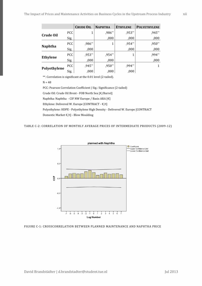
The Impact of Prices and Maintenance Activities on Business Cycles in the Upstream Process Industry xii
David Brandstädter | [email protected] Jul 2013
CRUDE OIL NAPHTHA ETHYLENE POLYETHYLENE
Crude Oil PCC 1 ,986** ,953** ,945** Sig. ,000 ,000 ,000
Naphtha PCC ,986** 1 ,954** ,950** Sig. ,000 ,000 ,000
Ethylene PCC ,953** ,954** 1 ,994** Sig. ,000 ,000 ,000
Polyethylene PCC ,945** ,950** ,994** 1 Sig. ,000 ,000 ,000
**. Correlation is significant at the 0.01 level (2-tailed).
N = 48
PCC: Pearson Correlation Coefficient | Sig.: Significance (2-tailed)
Crude Oil: Crude Oil Brent - FOB North Sea [€/Barrel]
Naphtha: Naphtha - CIF NW Europe / Basis ARA [€]
Ethylene: Delivered W. Europe [CONTRACT - €/t]
Polyethylene: HDPE - Polyethylene High Density - Delivered W. Europe [CONTRACT
Domestic Market €/t] - Blow Moulding
TABLE C-2: CORRELATION OF MONTHLY AVERAGE PRICES OF INTERMEDIATE PRODUCTS (2009-12)
FIGURE C-1: CROSSCORRELATION BETWEEN PLANNED MAINTENANCE AND NAPHTHA PRICE

xiii Appendices
Master Thesis TU/e Eindhoven
HDPE - BLOW
MOULDING
HDPE - HMW FILM
HDPE - INJECTION MOULDING
LLDPE - BUTENE,
FILM
LLDPE - OCTENE,
FILM
LDPE - FILM
HDPE - Blow Mold.
PCC 1 ,998** ,997** ,942** ,916** ,944**
Sig. .000 .000 .000 .000 .000
HDPE - HMW Film
PCC ,998** 1 ,994** ,943** ,910** ,946**
Sig. .000 .000 .000 .000 .000
HDPE – Inject. Mold.
PCC ,997** ,994** 1 ,943** ,932** ,952**
Sig. .000 .000 .000 .000 .000
LLDPE – But., Film
PCC ,942** ,943** ,943** 1 ,962** ,988**
Sig. .000 .000 .000 .000 .000
LLDPE – Oct., Film
PCC ,916** ,910** ,932** ,962** 1 ,972**
Sig. .000 .000 .000 .000 .000
LDPE - Film
PCC ,944** ,946** ,952** ,988** ,972** 1
Sig. .000 .000 .000 .000 .000 **. Correlation is significant at the 0.01 level (2-tailed). N = 96 PCC: Pearson Correlation Coefficient | Sig.: Significance (2-tailed) HDPE - Blow Moulding: Polyethylene High Density - Delivered W. Europe [CONTRACT Domestic Market €/t] - Blow Moulding HDPE - HMW Film: Polyethylene High Density - Delivered W. Europe [CONTRACT Domestic Market €/t] - HMW Film HDPE - Injection Moulding: Polyethylene High Density - Delivered W. Europe [CONTRACT Domestic Market €/t] - Injection Moulding LLDPE - Butene, Film: Polyethylene Linear Low Density - Delivered W. Europe [CONTRACT Domestic Market €/t] - Butene, Film LLDPE - Octene, Film: Polyethylene Linear Low Density - Delivered W. Europe [CONTRACT Domestic Market €/t] - Octene, Film LDPE - GP-Film: Polyethylene Low Density - Delivered W. Europe [CONTRACT Domestic Market €/t] - GP-Film
TABLE C-3: CORRELATION OF POLYETHYLENE PRICES

The Impact of Prices and Maintenance Activities on Business Cycles in the Upstream Process Industry xiv
David Brandstädter | [email protected] Jul 2013
COEFFICIENTS
Model Unstandardized
Coefficients Standardized Coefficients t Sig.
B Std. Error Beta
1 (Constant) 405,172 14,474 27,993 ,000
planned ,858 ,235 ,478 3,647 ,001
2
(Constant) 229,966 33,093 6,949 ,000
planned ,665 ,185 ,370 3,601 ,001
Crude Oil Brent - FOB North Sea [€/Barrel]
2,678 ,476 ,578 5,624 ,000
3
(Constant) 246,850 39,757 6,209 ,000
planned ,676 ,186 ,377 3,635 ,001
Crude Oil Brent - FOB North Sea [€/Barrel]
2,429 ,576 ,525 4,217 ,000
Quarterly GDP Western Europe
3,035 3,920 ,095 ,774 ,443
4
(Constant) 167,439 48,911 3,423 ,001
planned ,559 ,181 ,311 3,082 ,004
Crude Oil Brent - FOB North Sea [€/Barrel]
1,628 ,629 ,352 2,589 ,013
Quarterly GDP Western Europe
1,478 3,746 ,046 ,395 ,695
Ethylene Spread -1 ,319 ,126 ,330 2,527 ,015
Dependent Variable: SPREAD Ethylene - Delivered W. Europe [CONTRACT] DELTA Naphtha
TABLE C-4: REGRESSION COEFFICIENTS - MAINTENANCE PRICE MODEL
MODEL R R
SQUARE ADJUSTED
R SQUARE STD. ERROR OF THE
ESTIMATE
CHANGE STATISTICS R SQUARE
CHANGE F CHANGE SIG. F CHANGE 1 ,680a ,462 ,450 61,5401179 ,462 39,477 ,000
2 ,766b ,587 ,569 54,4867509 ,125 13,680 ,001
a. Predictors: (Constant), Crude Oil Brent - FOB North Sea [€/Barrel]
b. Predictors: (Constant), Crude Oil Brent - FOB North Sea [€/Barrel], planned
TABLE C-5: SWAPPED ORDER IN THE ETHYLENE REGRESSION MODEL

xv Appendices
Master Thesis TU/e Eindhoven
COEFFICIENTS
Model Unstandardized
Coefficients Standardized Coefficients t Sig.
B Std. Error Beta
1 (Constant) 605,001 15,335 39,452 ,000
planned 1,080 ,252 ,534 4,286 ,000
2
(Constant) 415,596 32,741 12,693 ,000
planned ,823 ,192 ,407 4,286 ,000
Crude Oil Brent - FOB North Sea
[€/Barrel]
2,954 ,479 ,586 6,172 ,000
3
(Constant) 430,854 40,958 10,519 ,000
planned ,830 ,194 ,411 4,288 ,000
Crude Oil Brent - FOB North Sea
[€/Barrel]
2,732 ,597 ,542 4,573 ,000
Quarterly GDP Western Europe 2,537 4,042 ,073 ,628 ,533
Dependent Variable: SPREAD HDPE - Polyethylene High Density - Delivered W. Europe [CONTRACT Domestic
Market €/t] - Blow Moulding
TABLE C-6: REGRESSION COEFFICIENTS CRUDE OIL LAG -1
MODEL R R SQUARE ADJUSTED R
SQUARE STD. ERROR OF
THE ESTIMATE DURBIN-WATSON 1 ,986a ,973 ,972 2,96416 ,657
a. Predictors: (Constant), Naphtha - CIF NW Europe / Basis ARA [€]
b. Dependent Variable: Crude Oil Brent - FOB North Sea [€/Barrel]
MODEL R R SQUARE ADJUSTED R
SQUARE STD. ERROR OF
THE ESTIMATE DURBIN-WATSON 1 ,953a ,907 ,905 5,43940 1,143
a. Predictors: (Constant), Ethylene - Delivered W. Europe [CONTRACT - €/t]
b. Dependent Variable: Crude Oil Brent - FOB North Sea [€/Barrel]
MODEL R R SQUARE ADJUSTED R
SQUARE STD. ERROR OF
THE ESTIMATE DURBIN-WATSON 1 ,945a ,893 ,891 5,83834 ,988
a. Predictors: (Constant), HDPE - Polyethylene High Density - Delivered W. Europe [CONTRACT Domestic Market
€/t] - Blow Moulding
b. Dependent Variable: Crude Oil Brent - FOB North Sea [€/Barrel]
TABLE C-7: REGRESSION MODELS ON OIL PRICE

The Impact of Prices and Maintenance Activities on Business Cycles in the Upstream Process Industry xvi
David Brandstädter | [email protected] Jul 2013
Appendix D SUPPLY CHAIN MODEL TESTS
PAIRED SAMPLES TEST
Paired Differences
t df
Sig. (2-
tailed) Mean
Std.
Deviation
Std. Error
Mean
99% Confidence
Interval of the
Difference
Lower Upper
Pair
1
InvCoverage_Period1 -
InvCoverage_Period2 > 0 ,83718 ,17089 ,5440 1,5034 > 0 23 ,000
Pair
2
InvCoverage_Period1 -
InvCoverage_Period3 > 0 1,11411 ,22742 -,4180 ,8588 > 0 23 ,343
Pair
3
InvCoverage_Period2 -
InvCoverage_Period3 < 0 ,83590 ,17063 -1,2823 -,3243 < 0 23 ,000
TABLE D-1: T-TESTS FOR INVENTORY COVERAGE
Structural Assessment Test
As the model is triggered by end market demand, its structural integrity is tested by stepwise adding end market data. In total 14 end markets with distinct data sets are defined (see Figure A-4). As the model is based on normalised data it has its equilibrium if all end market demand equals 100. The two desired stock coverage adjustments of Echelon 3 are incorporated (see 5.1.2).
FIGURE D-1: STRUCTURAL ASSESSMENT TEST FOR END MARKETS
Figure D-1 shows the behaviour of feedstock orders (𝑂4) from the point when all end markets have a demand of 100 (then 𝑂4 = 100) to the point when all markets show the observed demand. The model behaves correctly, leaving its equilibrium and reacting in different sensitivity (based on the splits, see Table F-4: Theta split values) to the end markets.
0
20
40
60
80
100
120
Jan07
Jun07
Nov07
Apr08
Sep08
Feb09
Jun09
Nov09
Apr10
Sep10
Feb11
Jul11
Nov11
Apr12
Sep12
[Uni
ts/W
eek]
4 Feedstock Orders (Structural Assessment Test) All Demand = 100Demand +1Demand +2Demand +3Demand +4Demand +5Demand +6Demand +7Demand +8Demand +9Demand +10Demand +11Demand +12Demand +13Demand +14Demand +15

xvii Appendices
Master Thesis TU/e Eindhoven
Pulse Test
A pulse test is a test in which the model is exposed to a single pulse. To measure the oscillation factor, the model is initialised in equilibrium. All demand is set to 100 units/week. Then at time 10, end market demand is increased by 10% to 110 units/week. Figure D-2 shows the behaviour of the model. The highest echelon, Echelon 4, orders a maximum of 139.14 units/week, a plus of 40% and an oscillation factor of almost 4. This is due to the multiple information and material delays in the model. The overshoot after incorporation of demand is not severe but the prior reaction to the pulse is phased indicating an absorption process between Echelon 4 and 1. The two dents in the equilibrium series stem from the desired inventory coverage adjustment as discussed in 5.1.2. Note that in the pulse test the model has not swung back in its equilibrium until the first inventory adjustment more than one year later.
FIGURE D-2: RESULTS OF PULSE TEST (+10% DEMAND AT TIME 10)
Extreme Condition Test
An extreme conditions test probes the model’s robustness in extreme, often unrealistic condition. Three scenarios were tested: A High Demand scenario with a constant end market demand of 1000 units/week, a No Demand scenario27 with a constant end market demand of 1 unit/week and an Extreme Fluctuation scenario in which the demand is in a stable equilibrium of 100 units/week then drops to 10 units/week only to later skyrocket at 1000 units/week.
27 Due to ratio auxiliary variables (e.g. delivery ratio 𝑅𝑛), a demand of zero would result in division errors.
60
70
80
90
100
110
120
130
140
150
Jan07
Jun07
Nov07
Apr08
Sep08
Feb09
Jun09
Nov09
Apr10
Sep10
Feb11
Jul11
Nov11
Apr12
Sep12
[Uni
ts/W
eek]
4 - Feedstock Orders (Pulse Test)
Pulse Equilibrium

The Impact of Prices and Maintenance Activities on Business Cycles in the Upstream Process Industry xviii
David Brandstädter | [email protected] Jul 2013
FIGURE D-3: RESULTS OF EXTREME CONDITION TESTS
Figure D-3 shows the behaviour of the model. In fact, the extreme scenario led to a situation in which the backlogs became zero and hence the delivery ratio caused an error. To fix this, 0.0001 is added to the ratio. The model behaves as supposed. In particular the inventory levels are non-negative at all times and the model does not explode at any time.
SPREAD
HDPE
IMPORTS LLDPE
IMPORTS LDPE
IMPORTS TOTAL PE
IMPORTS Spread PCC 1 ,233 ,471** ,103 ,447**
Sig. ,111 ,001 ,488 ,001
HDPE Imports PCC ,233 1 ,155 ,529** ,781**
Sig. ,111 ,293 ,000 ,000
LLDPE Imports PCC ,471** ,155 1 -,073 ,679**
Sig. ,001 ,293 ,620 ,000
LDPE Imports PCC ,103 ,529** -,073 1 ,547**
Sig. ,488 ,000 ,620 ,000
Total PE Imports PCC ,447** ,781** ,679** ,547** 1
Sig. ,001 ,000 ,000 ,000 **. Correlation is significant at the 0.01 level (2-tailed).
N = 48
PCC: Pearson Correlation Coefficient | Sig.: Significance (2-tailed)
TABLE D-2: CORRELATIONS OF DIFFERENT POLYETHYLENE IMPORT VOLUMES ON PRICE SPREAD
-
1,000
2,000
3,000
4,000
Jan07
Nov07
Sep08
Jun09
Apr10
Feb11
Nov11
Sep12
[Uni
ts/W
eek]
4 - Stock C2
No Demand Equilibrium
-
500
1,000
1,500
2,000
Jan07
Nov07
Sep08
Jun09
Apr10
Feb11
Nov11
Sep12
[Uni
ts/W
eek]
4 - Feedstock Orders
High Demand Extreme Fluctutation
Extreme Condition Tests

xix Appendices
Master Thesis TU/e Eindhoven
MODEL R R
SQUARE ADJUSTED
R SQUARE
STD. ERROR
OF THE
ESTIMATE
CHANGE STATISTICS R SQUARE
CHANGE F
CHANGE DF1 DF2 SIG. F
CHANGE 1 ,534a ,285 ,270 76,26049113 ,285 18,373 1 46 ,000
2 ,832b ,693 ,679 50,54498526 ,407 59,713 1 45 ,000
3 ,833c ,694 ,673 51,05476729 ,001 ,106 1 44 ,746
a. Predictors: (Constant), Planned
b. Predictors: (Constant), Planned, Crude (-1)
c. Predictors: (Constant), Planned, Crude (-1), Total PE Imports (-1) [Dec 08]
TABLE D-3: REGRESSION MODEL INCLUDING POLYETHYLENE IMPORTS
FIGURE D-4: CROSS-CORRELATION LLDPE IMPORTS AND PRODUCTION
FIGURE D-5: CROSS-CORRELATION PRICE SPREAD WITH TOTAL PE IMPORTS

The Impact of Prices and Maintenance Activities on Business Cycles in the Upstream Process Industry xx
David Brandstädter | [email protected] Jul 2013
HDPE_IMP LDPE_IMP LLDPE_IMP HDPE_STOCK LDPESTOCK LLDPESTOCK HDPE_Imp PCC 1 ,474** -,011 -,300* -,234* ,032
Sig. ,000 ,924 ,010 ,048 ,787
LDPE_Imp PCC ,474** 1 -,305** -,481** -,459** -,324**
Sig. ,000 ,009 ,000 ,000 ,006
LLDPE_Imp PCC -,011 -,305** 1 ,487** ,566** ,453**
Sig. ,924 ,009 ,000 ,000 ,000
HDPE_Stock PCC -,300* -,481** ,487** 1 ,731** ,542**
Sig. ,010 ,000 ,000 ,000 ,000
LDPEstock PCC -,234* -,459** ,566** ,731** 1 ,569**
Sig. ,048 ,000 ,000 ,000 ,000
LLDPEstock PCC ,032 -,324** ,453** ,542** ,569** 1
Sig. ,787 ,006 ,000 ,000 ,000 **. Correlation is significant at the 0.01 level (2-tailed).
*. Correlation is significant at the 0.05 level (2-tailed).
N = 72
PCC: Pearson Correlation Coefficient | Sig.: Significance (2-tailed)
TABLE D-4: CORRELATION OF IMPORTS AND STOCKS
METRIC DEFINITION FORMULA VALUE
𝑅² Variance explained �1𝑛�
(𝑋𝑑 − 𝑋𝑑����)(𝑋𝑚 − 𝑋𝑚����)𝑠𝑑𝑠𝑚
�2
0.830
𝑀𝐴𝐸 Mean absolute error
1𝑛� |𝑋𝑚 − 𝑋𝑑 | 2.81
𝑀𝐴𝑃𝐸 Mean abslute percent error
1𝑛�
|𝑋𝑚 − 𝑋𝑑|𝑋𝑑
2.86%
𝑀𝐴𝐸𝑀𝑒𝑎𝑛
MAE as fraction of mean
𝑀𝐴𝐸𝑋𝑑����
2.86%
𝑅𝑀𝑆𝐸 Root Mean Square Error �1
𝑛�(𝑋𝑚 − 𝑋𝑑)2
3.48
Theil’s Inequality Statistics
𝑈𝑀 bias 𝑈𝑀 =(𝑋𝑚���� − 𝑋𝑑����)2
𝑀𝑆𝐸
0.002
𝑈𝑆 unequal variation 𝑈𝑆 =(𝑠𝑚 − 𝑠𝑑)2
𝑀𝑆𝐸
0.010
𝑈𝐶 unequal covariation 𝑈𝐶 =2�1 − √𝑅2�𝑠𝑚𝑠𝑑
𝑀𝑆𝐸
0.988
𝑑: observed data 𝑚: modelled data 𝑋: value 𝑋�: mean 𝑠: standard deviation
TABLE D-5: BEHAVIOUR REPRODUCTION STATISTICS FOR MODEL M2A

xxi Appendices
Master Thesis TU/e Eindhoven
Appendix E MODEL M1A CAPACITY LIMITATION ANALYSIS
To test the model’s behaviour under fictitious tighter capacity constraints, the nameplate capacity is artificially lowered by 15% after Lehman Shock. This is equivalent to 𝑢𝑛𝑝𝑙𝑎𝑛𝑛𝑒𝑑 𝑓𝑎𝑐𝑡𝑜𝑟 = 0.85. The modelled ethylene production is smoothened and less volatile than in the “uncapacitated” situation. However, in the end of 2012 production collapses in a severe trough and recovers equally sudden.
FIGURE E-1: ETHYLENE PRODUCTION UNDER ARTIFICIAL CAPACITY CONSTRAINT
The reason for this behaviour is a large amount of unfulfilled orders due to limited stock. The increased demand leads to an increase in forecasted orders which leads to an increase of feedstock orders. Because the production capacity is reached, finished inventory stock does not adjust to the new desired stock level leading to additional feedstock orders. Once demand cools the backlog is reduced. However, the excess orders are still in the production process and do not meet sufficient demand once finished. Thus orders are reduced and, via lower WIP stocks, lead to a production reduction.
60
80
100
120
140
Jan 07 Nov 07 Sep 08 Jun 09 Apr 10 Feb 11 Nov 11 Sep 12
[Uni
ts/W
eek]
4 - C2 acquisition rate (85% Capacity Limitation)
85% capacity uncapacitated

The Impact of Prices and Maintenance Activities on Business Cycles in the Upstream Process Industry xxii
David Brandstädter | [email protected] Jul 2013
FIGURE E-2: BEHAVIOUR OF KEY STOCKS UNDER FICTICIOUS CAPACITY (ECHELON 4)
Whereas it is unlikely that capacity reduction is not taken into account in the order decision, this artificial experiment shows the inertia of complex systems in particular in times of high utilisation. In addition, it shows comprehensible behaviour of the model underlying its asserted robustness (see 5.1.3).
60
80
100
120
140
Jan07
Nov07
Sep08
Jun09
Apr10
Feb11
Nov11
Sep12
[Uni
ts/W
eek]
4 - Forecast Chemicals
85% capacity uncapacitated
-
50
100
150
200
Jan07
Nov07
Sep08
Jun09
Apr10
Feb11
Nov11
Sep12
[Uni
ts/W
eek]
4 - Stock C2
85% capacity uncapacitated
60
80
100
120
140
Jan07
Nov07
Sep08
Jun09
Apr10
Feb11
Nov11
Sep12
[Uni
ts/W
eek]
4 - Feedstock Orders
85% capacity uncapacitated
-
100
200
300
400
Jan07
Nov07
Sep08
Jun09
Apr10
Feb11
Nov11
Sep12
[Uni
ts/W
eek]
4 - Backlog C2 Orders
85% capacity uncapacitated
85% Capacity Limitation

xxiii Appendices
Master Thesis TU/e Eindhoven
Appendix F SUPPLY CHAIN MODEL PARAMETERS
ECHELON TYPE ESTIMATED
VALUE [WEEKS]
TOLERANCE BAND (± 25%)
CALIBRATED VALUE
[WEEKS] LOWER UPPER 2.1 Transportation Lead time 0.25 0.19 0.31 0.20 2.1 Desired inventory coverage 7.00 5.25 8.75 6.12 2.1 Order fulfil delay 1.00 0.75 1.25 1.11 2.1 Product delivery time 1.00 0.75 1.25 1.25 2.1 Production time 2.00 1.50 2.50 1.71 2.2 Transportation Lead time 0.25 0.19 0.31 0.30 2.2 Desired inventory coverage 7.00 5.25 8.75 5.26 2.2 Order fulfil delay 1.00 0.75 1.25 1.00 2.2 Product delivery time 1.00 0.75 1.25 1.12 2.2 Production time 2.00 1.50 2.50 1.50 2.3 Transportation Lead time 0.25 0.19 0.31 0.30 2.3 Desired inventory coverage 7.00 5.25 8.75 7.04 2.3 Order fulfil delay 1.00 0.75 1.25 1.00 2.3 Product delivery time 1.00 0.75 1.25 1.25 2.3 Production time 2.00 1.50 2.50 2.50 1.1.1 Transportation Lead time 1.00 0.75 1.25 1.23 1.1.1 Desired inventory coverage 8.00 6.00 10.00 10.00 1.1.1 Order fulfil delay 1.00 0.75 1.25 0.75 1.1.1 Product delivery time 1.00 0.75 1.25 1.19 1.1.1 Production time 3.00 2.25 3.75 3.75 1.1.2 Transportation Lead time 1.00 0.75 1.25 0.76 1.1.2 Desired inventory coverage 8.00 6.00 10.00 7.45 1.1.2 Order fulfil delay 1.00 0.75 1.25 0.75 1.1.2 Product delivery time 1.00 0.75 1.25 1.25 1.1.2 Production time 3.00 2.25 3.75 3.05 1.1.4 Transportation Lead time 1.00 0.75 1.25 1.24 1.1.4 Desired inventory coverage 8.00 6.00 10.00 6.00 1.1.4 Order fulfil delay 1.00 0.75 1.25 1.00 1.1.4 Product delivery time 1.00 0.75 1.25 1.25 1.1.4 Production time 3.00 2.25 3.75 3.75 1.2.1 Transportation Lead time 1.00 0.75 1.25 0.75 1.2.1 Desired inventory coverage 8.00 6.00 10.00 6.06 1.2.1 Order fulfil delay 1.00 0.75 1.25 1.03 1.2.1 Product delivery time 1.00 0.75 1.25 1.25 1.2.1 Production time 3.00 2.25 3.75 3.74 1.2.2 Transportation Lead time 1.00 0.75 1.25 1.25 1.2.2 Desired inventory coverage 8.00 6.00 10.00 10.00 1.2.2 Order fulfil delay 1.00 0.75 1.25 1.00 1.2.2 Product delivery time 1.00 0.75 1.25 0.75 1.2.2 Production time 3.00 2.25 3.75 3.75 1.3.1 Transportation Lead time 1.00 0.75 1.25 0.76 1.3.1 Desired inventory coverage 8.00 6.00 10.00 6.01 1.3.1 Order fulfil delay 1.00 0.75 1.25 1.03 1.3.1 Product delivery time 1.00 0.75 1.25 1.25 1.3.1 Production time 3.00 2.25 3.75 3.75 1.3.2 Transportation Lead time 1.00 0.75 1.25 0.80 1.3.2 Desired inventory coverage 8.00 6.00 10.00 6.01 1.3.2 Order fulfil delay 1.00 0.75 1.25 1.03 1.3.2 Product delivery time 1.00 0.75 1.25 1.25 1.3.2 Production time 3.00 2.25 3.75 2.30
TABLE F-1: OBSERVABLE PARAMETERS OF THE BASIC SUPPLY CHAIN MODEL

The Impact of Prices and Maintenance Activities on Business Cycles in the Upstream Process Industry xxiv
David Brandstädter | [email protected] Jul 2013
ECHELON TYPE VALUE IN
LITERATURE [WEEKS]
CALIBRATED VALUE
[WEEKS] 2.1 Supply Line Adjustment time 1000 1.28 2.1 WIP adjustment time 1000 999.70 2.1 Forecast adjustment time 100 11.89 2.1 Stock adjustment time 10 2.12 2.2 Supply Line Adjustment time 1000 668.15 2.2 WIP adjustment time 1000 8.40 2.2 Forecast adjustment time 100 15.00 2.2 Stock adjustment time 10 1.09 2.3 Supply Line Adjustment time 1000 989.98 2.3 WIP adjustment time 1000 1.00 2.3 Forecast adjustment time 100 1.18 2.3 Stock adjustment time 10 7.83 1.1.1 Supply Line Adjustment time 1.02 1.1.1 WIP adjustment time 1.91 1.1.1 Forecast adjustment time 99.81 1.1.1 Stock adjustment time 3.48 1.1.2 Supply Line Adjustment time 26.51 1.1.2 WIP adjustment time 1.00 1.1.2 Forecast adjustment time 69.15 1.1.2 Stock adjustment time 13.44 1.1.4 Supply Line Adjustment time 1,000.00 1.1.4 WIP adjustment time 995.16 1.1.4 Forecast adjustment time 6.02 1.1.4 Stock adjustment time 4.72 1.2.1 Supply Line Adjustment time 1.68 1.2.1 WIP adjustment time 904.68 1.2.1 Forecast adjustment time 100.00 1.2.1 Stock adjustment time 15.00 1.2.2 Supply Line Adjustment time 17.15 1.2.2 WIP adjustment time 958.83 1.2.2 Forecast adjustment time 2.71 1.2.2 Stock adjustment time 2.07 1.3.1 Supply Line Adjustment time 754.47 1.3.1 WIP adjustment time 1.00 1.3.1 Forecast adjustment time 100.00 1.3.1 Stock adjustment time 14.95 1.3.2 Supply Line Adjustment time 37.61 1.3.2 WIP adjustment time 6.95 1.3.2 Forecast adjustment time 1.00 1.3.2 Stock adjustment time 1.92
TABLE F-2: BEHAVIOURAL PARAMETERS OF THE BASIC SUPPLY CHAIN MODEL
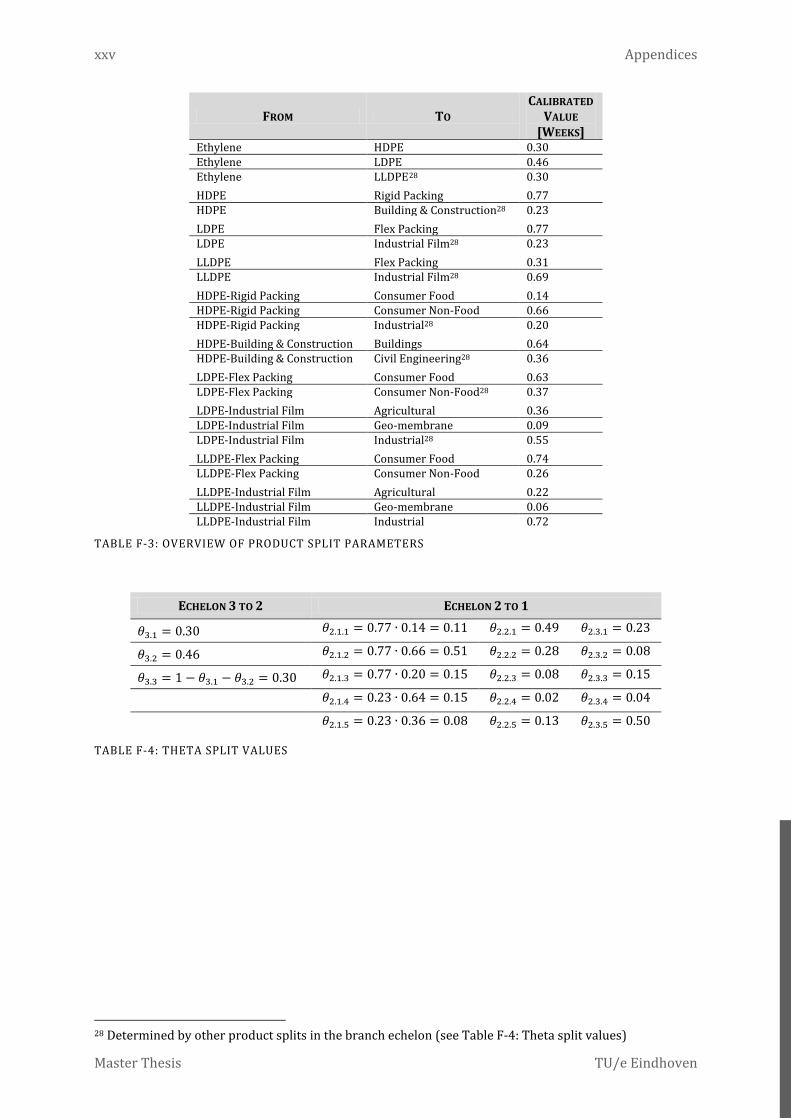
xxv Appendices
Master Thesis TU/e Eindhoven
FROM TO CALIBRATED
VALUE [WEEKS]
Ethylene HDPE 0.30 Ethylene LDPE 0.46 Ethylene LLDPE28 0.30
HDPE Rigid Packing 0.77 HDPE Building & Construction28 0.23
LDPE Flex Packing 0.77 LDPE Industrial Film28 0.23
LLDPE Flex Packing 0.31 LLDPE Industrial Film28 0.69
HDPE-Rigid Packing Consumer Food 0.14 HDPE-Rigid Packing Consumer Non-Food 0.66 HDPE-Rigid Packing Industrial28 0.20
HDPE-Building & Construction Buildings 0.64 HDPE-Building & Construction Civil Engineering28 0.36
LDPE-Flex Packing Consumer Food 0.63 LDPE-Flex Packing Consumer Non-Food28 0.37
LDPE-Industrial Film Agricultural 0.36 LDPE-Industrial Film Geo-membrane 0.09 LDPE-Industrial Film Industrial28 0.55
LLDPE-Flex Packing Consumer Food 0.74 LLDPE-Flex Packing Consumer Non-Food 0.26
LLDPE-Industrial Film Agricultural 0.22 LLDPE-Industrial Film Geo-membrane 0.06 LLDPE-Industrial Film Industrial 0.72
TABLE F-3: OVERVIEW OF PRODUCT SPLIT PARAMETERS
ECHELON 3 TO 2 ECHELON 2 TO 1
𝜃3.1 = 0.30 𝜃2.1.1 = 0.77 ∙ 0.14 = 0.11 𝜃2.2.1 = 0.49 𝜃2.3.1 = 0.23
𝜃3.2 = 0.46 𝜃2.1.2 = 0.77 ∙ 0.66 = 0.51 𝜃2.2.2 = 0.28 𝜃2.3.2 = 0.08
𝜃3.3 = 1 − 𝜃3.1 − 𝜃3.2 = 0.30 𝜃2.1.3 = 0.77 ∙ 0.20 = 0.15 𝜃2.2.3 = 0.08 𝜃2.3.3 = 0.15
𝜃2.1.4 = 0.23 ∙ 0.64 = 0.15 𝜃2.2.4 = 0.02 𝜃2.3.4 = 0.04
𝜃2.1.5 = 0.23 ∙ 0.36 = 0.08 𝜃2.2.5 = 0.13 𝜃2.3.5 = 0.50
TABLE F-4: THETA SPLIT VALUES
28 Determined by other product splits in the branch echelon (see Table F-4: Theta split values)

The Impact of Prices and Maintenance Activities on Business Cycles in the Upstream Process Industry xxvi
David Brandstädter | [email protected] Jul 2013
PARAMETER 95% PAYOFF VALUE CONFIDENCE INTERVAL LOWER BOUND ACTUAL VALUE UPPER BOUND
4 Feedstock transport lead time 0.55 0.55 0.55 4 Desired C2 inventory coverage 0.75* 0.75 0.75 4 Order fulfill delay 0.63 0.63 0.63* 4 C2 delivery time 0.38 0.38 0.47 4 C2 production time 0.61* 0.63 0.63* 3 C2 transportation lead time 1.23 1.24 1.25 3 Desired PE inventory coverage I 5.59* 5.59 5.59* 3 Desired PE inventory coverage II 4.56* 4.56 4.56* 3 Desired PE inventory coverage III 5.37* 5.37 5.37* 3 Order fulfill delay 0.38* 0.50 0.63* 3 PE delivery time 0.38* 0.38 0.39 3 PE production time 3.74 3.75 3.75* 2.1 HDPE transportation lead time 0.19 0.20 0.20 2.1 Desired HDPE-product inventory coverage 6.12 6.15 6.17 2.1 Order fulfill delay 1.05 1.06 1.08 2.1 HDPE delivery time 1.22 1.25 1.25* 2.1 HDPE production time 1.76 1.79 1.81 2.2 LDPE transportation lead time 0.19* 0.30 0.31* 2.2 Desired LDPE-product inventory coverage 5.25* 5.27 7.03 2.2 Order fulfill delay 0.75* 1.00 1.25* 2.2 LDPE delivery time 1.07 1.12 1.16 2.2 LDPE production time 1.50* 1.50 2.00 2.3 LLDPE transportation lead time 0.27 0.30 0.31* 2.3 Desired LLDPE-product inventory coverage 6.50 7.06 7.62 2.3 Order fulfill delay 0.75* 1.00 1.25* 2.3 LLDPE delivery time 1.06 1.24 1.25* 2.3 LLDPE production time 2.44 2.50 2.50* 1.1.1 HDPE-Product transportation lead time 1.05 1.25 1.25* 1.1.1 Desired OEM 1.1 inventory coverage 9.70 10.00 10.00* 1.1.1 Order fulfill delay 0.75* 0.75 1.13 1.1.1 Final Product delivery time 0.75* 1.20 1.25* 1.1.1 OEM 1.1 production time 3.22 3.75 3.75* 1.1.2 HDPE-Product transportation lead time 0.75* 0.76 0.77 1.1.2 Desired OEM 1.2 inventory coverage 7.16 7.26 7.37 1.1.2 Order fulfill delay 0.75* 0.75 0.84 1.1.2 Final Product delivery time 0.75* 1.25 1.25* 1.1.2 OEM 1.2 production time 2.94 2.97 2.99 1.1.4 HDPE-Product transportation lead time 1.23 1.24 1.25* 1.1.4 Desired OEM 1.4 inventory coverage 6.00* 6.00 6.14 1.1.4 Order fulfill delay 0.75* 1.00 1.25* 1.1.4 Final Product delivery time 1.14 1.25 1.25* 1.1.4 OEM 1.4 production time 3.73 3.75 3.75* 1.2.1 LDPE-Product transportation lead time 0.75* 0.75 1.25* 1.2.1 Desired OEM 2.1 inventory coverage 6.00* 6.67 10.00* 1.2.1 Order fulfill delay 0.75* 1.03 1.25* 1.2.1 Final Product delivery time 0.75* 1.25 1.25* 1.2.1 OEM 2.1 production time 2.25* 3.74 3.75* 1.2.2 LDPE-Product transportation lead time 1.20 1.24 1.25* 1.2.2 Desired OEM 2.2 inventory coverage 9.55 10.00 10.00* 1.2.2 Order fulfill delay 0.75* 1.00 1.25* 1.2.2 Final Product delivery time 0.75* 0.75 1.14 1.2.2 OEM 2.2 production time 3.69 3.75 3.75* 1.3.1 LLDPE-Product transportation lead time 0.75* 0.76 1.25* 1.3.1 Desired OEM 3.1 inventory coverage 6.00* 6.15 10.00* 1.3.1 Order fulfill delay 0.75* 1.00 1.25* 1.3.1 Final Product delivery time 0.75* 1.23 1.25* 1.3.1 OEM 3.1 production time 2.25* 2.27 3.75* 1.3.2 LLDPE-Product Transportation lead time 0.75* 0.80 0.95 1.3.2 Desired OEM 3.2 inventory coverage 6.00* 6.01 6.91 1.3.2 Order fulfill delay 0.75* 1.03 1.25* 1.3.2 Final Product delivery time 0.75* 1.25 1.25* 1.3.2 OEM 3.2 production time 2.25* 2.31 2.58

xxvii Appendices
Master Thesis TU/e Eindhoven
4 Supply Line Adjustment Time 1.02 1.12 1.20 4 WIP adjustment time of feedstock orders 33.32 962.01 1,000.00* 4 C2 forecast adjustment time 6.54 6.72 6.98 4 C2 stock adjustment time 2.79 2.88 2.95 3 Supply Line Adjustment Time 538.82 1,000.00 1,000.00* 3 WIP adjustment time of C2 orders 563.28 1,000.00 1,000.00* 3 PE forecast adjustment time 9.59 10.21 10.76 3 PE stock adjustment time 7.08 7.17 7.19 2.1 Supply Line Adjustment Time 1.28 1.28 1.29 2.1 WIP adjustment time of HDPE orders 164.46 996.81 1,000.00* 2.1 HDPE forecast adjustment time 7.78 7.83 7.89 2.1 HDPE-product stock adjustment time 11.82 11.88 11.93 2.2 Supply Line Adjustment Time 1.95 2.12 2.41 2.2 WIP adjustment time of LDPE orders 17.04 616.44 1,000.00* 2.2 LDPE forecast adjustment time 7.56 8.01 8.60 2.2 LDPE-product stock adjustment time 13.78 15.00 15.00* 2.3 Supply Line Adjustment Time 1.00* 1.09 1.23 2.3 WIP adjustment time of LLDPE orders 42.57 949.12 1,000.00* 2.3 LLDPE forecast adjustment time 1.00* 1.00 1.09 2.3 LLDPE-product stock adjustment time 1.12 1.18 1.24 1.1.1 Supply Line Adjustment Time 1.00* 1.02 1.07 1.1.1 WIP adjustment time of HDPE-product orders 1.54 1.91 2.13 1.1.1 OEM 1.1 forecast adjustment time 58.32 99.63 100.00* 1.1.1 OEM 1.1 stock adjustment time 3.39 3.62 3.86 1.1.2 Supply Line Adjustment Time 25.96 26.51 26.89 1.1.2 WIP adjustment time of HDPE-product orders 1.00* 1.00 1.01 1.1.2 OEM 1.2 forecast adjustment time 46.35 57.16 72.16 1.1.2 OEM 1.2 stock adjustment time 12.67 12.93 13.27 1.1.4 Supply Line Adjustment Time 715.02 999.90 1,000.00* 1.1.4 WIP adjustment time of HDPE-product orders 584.51 998.83 1,000.00* 1.1.4 OEM 1.4 forecast adjustment time 5.64 5.80 6.10 1.1.4 OEM 1.4 stock adjustment time 4.73 4.76 4.78 1.2.1 Supply Line Adjustment Time 1.00* 1.08 3.46 1.2.1 WIP adjustment time of LDPE-product orders 2.83 904.08 1,000.00* 1.2.1 OEM 2.1 forecast adjustment time 66.27 99.42 100.00* 1.2.1 OEM 2.1 stock adjustment time 9.83 14.80 15.00* 1.2.2 Supply Line Adjustment Time 15.23 16.61 18.53 1.2.2 WIP adjustment time of LDPE-product orders 159.43 995.27 1,000.00* 1.2.2 OEM 2.2 forecast adjustment time 2.36 2.71 2.93 1.2.2 OEM 2.2 stock adjustment time 2.04 2.07 2.09 1.3.1 Supply Line Adjustment Time 1.00* 766.16 1,000.00* 1.3.1 WIP adjustment time of LLDPE-product orders 1.00* 1.00 3.77 1.3.1 OEM 3.1 forecast adjustment time 51.57 100.00 100.00* 1.3.1 OEM 3.1 stock adjustment time 8.95 14.93 15.00* 1.3.2 Supply Line Adjustment Time 16.62 57.22 1,000.00* 1.3.2 WIP adjustment time of LLDPE-product orders 5.38 6.95 9.02 1.3.2 OEM 3.2 forecast adjustment time 1.00* 1.00 1.25 1.3.2 OEM 3.2 stock adjustment time 1.84* 1.92 2.03 Split: ETHYLENE to HDPE 0.30* 0.30 0.30 Split: ETHYLENE to LDPE 0.45 0.46 0.46* Split: HDPE to Rigid Packing 0.77 0.77 0.77 Split: LDPE to Flex Packing 0.76 0.77 0.78 Split: LLDPE to Flex Packing 0.31* 0.31 0.33 Split: HDPE-Rigid Packing to Consumer Food 0.14 0.14 0.15 Split: HDPE-Rigid Packing to Consumer Non-Food 0.68 0.68 0.68 Split: HDPE-Building & Construction to Buildings 0.65 0.66 0.66 Split: LDPE-Flex Packing to Consumer Food 0.61 0.63 0.65 Split: LDPE-Industrial to Agricultural 0.34 0.36 0.36* Split: LDPE-Industrial Film to Geo-membrane 0.06* 0.09 0.09* Split: LLDPE-Flex Packing to Consumer Food 0.72 0.74 0.74* Split: LLDPE-Industrial Film to Agricultural 0.22* 0.22 0.24 Split: LLDPE-Industrial Film to Geo-membrane 0.06* 0.06 0.09* * 95% confidence interval exceeds calibration limit
TABLE F-5: CONFIDENCE INTERVAL OF PARAMETERS

The Impact of Prices and Maintenance Activities on Business Cycles in the Upstream Process Industry xxviii
David Brandstädter | [email protected] Jul 2013
# LOCATION BEHAVIOURAL OBSERVABLE
1 Split: HDPE to Rigid Packing x
2 1.1.2 WIP adjustment time of HDPE-product orders x
3 1.1.4 OEM 1.4 stock adjustment time x
4 Split: HDPE-Building & Construction to Buildings x
5 2.1 Desired HDPE-product inventory coverage x
6 3 PE production time x
7 2.1 Supply Line Adjustment Time x
8 Split: HDPE-Rigid Packing to Consumer Non-Food x
9 3 Desired PE inventory coverage x
10 4 Desired C2 inventory coverage x
11 2.1 HDPE forecast adjustment time x
12 2.1 HDPE-product stock adjustment time x
13 4 Order fulfill delay x
14 1.1.2 OEM 1.2 production time x
15 1.2.2 OEM 2.2 stock adjustment time x
16 1.1.4 OEM 1.4 production time x
17 1.1.2 HDPE-Product transportation lead time x
18 Split: ETHYLENE to HDPE x
19 2.1 HDPE production time x
20 1.2.2 OEM 2.2 production time x
TABLE F-6: MOST SENSITIVE PARAMETERS OF MODEL M1A
Variable Run 1
RUN 2
RUN 3
RUN 4
RUN 5
RUN 6
RUN 7
RUN 8
RUN 9
RUN 10 𝝈 𝝁
𝝈𝝁 #TOP
R²-value .776 .791 .777 .794 .710 .720 .778 .794 .779 .785 0.03 0.77 0.04 50 25
4 Feedstock transport lead time 0.39 0.39 0.39 0.39 0.59 0.62 0.39 0.39 0.39 0.39 0.09 0.43 0.21 10 1
4 Desired C2 inventory coverage 1.25 1.25 1.25 1.25 0.75 0.75 1.25 1.25 1.25 1.25 0.21 1.15 0.18 10 3
4 Order fulfill delay 0.50 0.63 0.63 0.50 0.63 0.63 0.58 0.63 0.50 0.50 0.06 0.57 0.11 10 3
4 C2 delivery time 0.63 0.63 0.63 0.63 0.51 0.61 0.63 0.63 0.63 0.63 0.04 0.62 0.06 10 0
4 C2 production time 0.38 0.38 0.38 0.38 0.63 0.63 0.38 0.38 0.39 0.38 0.10 0.43 0.24 10 1
3 C2 transportation lead time 1.25 1.22 1.23 1.24 1.24 1.25 1.21 1.24 1.23 1.23 0.01 1.23 0.01 10 0
3 Desired PE inventory coverage I 5.59 5.59 5.59 5.59 6.15 6.15 5.59 5.59 5.59 5.59 0.24 5.70 0.04 10 10
3 Desired PE inventory coverage II 4.56 4.56 4.56 4.56 4.56 4.56 4.56 4.56 4.56 4.56 0.00 4.56 0.00 10 10
3 Desired PE inventory coverage III 5.37 5.37 5.37 5.37 5.37 5.37 5.37 5.37 5.37 5.37 0.00 5.37 0.00 10 10
3 Order fulfill delay 0.50 0.50 0.50 0.50 0.50 0.50 0.50 0.50 0.50 0.50 0.00 0.50 0.00 0 0
3 PE delivery time 0.42 0.38 0.38 0.58 0.63 0.63 0.39 0.58 0.44 0.38 0.11 0.48 0.23 10 7
3 PE production time 3.75 3.71 3.75 3.75 3.75 3.75 3.75 3.75 3.75 3.66 0.03 3.74 0.01 10 10
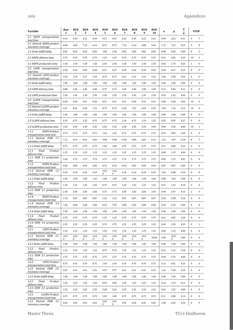
xxix Appendices
Master Thesis TU/e Eindhoven
Variable Run 1
RUN 2
RUN 3
RUN 4
RUN 5
RUN 6
RUN 7
RUN 8
RUN 9
RUN 10 𝝈 𝝁
𝝈𝝁 #TOP
2.1 HDPE transportation lead time 0.19 0.20 0.22 0.20 0.27 0.27 0.22 0.20 0.22 0.22 0.03 0.22 0.11 4 7
2.1 Desired HDPE-product inventory coverage 8.48 6.84 7.24 6.16 8.75 8.75 7.34 6.16 6.86 5.66 1.12 7.22 0.15 9 8
2.1 Order fulfill delay 0.82 0.82 0.82 0.82 1.00 1.00 0.82 0.82 0.82 0.82 0.08 0.85 0.09 0 5
2.1 HDPE delivery time 0.75 0.75 0.75 0.75 1.25 1.25 0.75 0.75 0.75 0.75 0.21 0.85 0.25 10 2
2.1 HDPE production time 1.50 1.50 1.50 1.50 2.50 2.50 1.50 1.50 1.50 1.50 0.42 1.70 0.25 1 0
2.2 LDPE transportation lead time 0.30 0.25 0.30 0.20 0.27 0.27 0.30 0.20 0.30 0.30 0.04 0.27 0.15 8 0
2.2 Desired LDPE-product inventory coverage 5.29 5.29 5.27 5.29 8.75 8.75 5.31 5.29 5.31 5.26 1.46 5.98 0.24 6 0
2.2 Order fulfill delay 1.00 1.00 1.00 1.00 1.00 1.00 1.00 1.00 1.00 1.00 0.00 1.00 0.00 0 0
2.2 LDPE delivery time 0.88 1.00 1.00 1.00 0.75 0.75 1.00 1.00 1.00 1.00 0.11 0.94 0.11 0 0
2.2 LDPE production time 2.20 2.49 2.38 2.49 2.50 2.50 2.39 2.49 2.39 2.38 0.09 2.42 0.04 9 0
2.3 LLDPE transportation lead time 0.30 0.30 0.31 0.30 0.31 0.31 0.31 0.30 0.31 0.31 0.00 0.30 0.02 10 0
2.3 Desired LLDPE-product inventory coverage 6.47 8.42 6.56 7.52 8.75 8.75 6.04 7.52 6.04 6.50 1.09 7.26 0.15 10 0
2.3 Order fulfill delay 1.00 1.00 1.00 1.00 1.00 1.00 1.00 1.00 1.00 1.00 0.00 1.00 0.00 0 0
2.3 LLDPE delivery time 0.76 0.75 1.25 0.75 0.75 0.75 1.24 0.75 1.24 1.25 0.25 0.95 0.27 9 0
2.3 LLDPE production time 2.50 2.50 2.50 2.50 2.50 2.50 2.50 2.50 2.50 2.50 0.00 2.50 0.00 10 1
1.1.1 HDPE-Product transportation lead time 0.75 0.75 0.75 0.75 1.24 1.24 0.75 0.75 0.75 0.75 0.21 0.85 0.24 0 0
1.1.1 Desired OEM 1.1 inventory coverage 7.72 6.91 8.31 6.85 9.98 9.98 9.20 6.85 6.81 6.14 1.41 7.87 0.18 8 7
1.1.1 Order fulfill delay 0.75 0.75 0.75 0.75 1.00 1.00 0.75 0.75 0.75 0.75 0.11 0.80 0.13 0 0
1.1.1 Final Product delivery time 1.25 1.25 1.25 1.25 1.25 1.25 1.25 1.25 1.25 1.25 0.00 1.25 0.00 0 0
1.1.1 OEM 1.1 production time 3.60 3.73 3.73 3.73 3.75 3.75 3.73 3.73 3.73 3.73 0.05 3.72 0.01 0 0
1.1.2 HDPE-Product transportation lead time 0.85 0.85 0.94 0.85 0.76 0.76 0.94 0.85 0.94 0.94 0.07 0.87 0.09 0 0
1.1.2 Desired OEM 1.2 inventory coverage 6.10 6.10 6.10 6.10 10.0
0 10.00 6.10 6.10 6.10 6.10 1.65 6.88 0.24 0 0
1.1.2 Order fulfill delay 1.00 1.00 1.00 1.25 1.00 1.00 1.00 1.00 1.00 1.00 0.08 1.03 0.08 0 0
1.1.2 Final Product delivery time 1.25 1.25 1.25 1.25 0.75 0.75 1.25 1.25 1.25 1.25 0.21 1.15 0.18 0 0
1.1.2 OEM 1.2 production time 2.38 2.83 2.83 2.83 3.75 3.75 2.83 2.83 2.83 2.83 0.44 2.97 0.15 2 4
1.1.4 HDPE-Product transportation lead time 1.18 0.87 0.87 0.87 1.25 1.25 0.87 0.87 0.87 0.87 0.18 0.98 0.18 0 0
1.1.4 Desired OEM 1.4 inventory coverage 7.04 6.00 6.00 6.00 6.65 7.53 6.00 6.00 6.00 6.00 0.56 6.32 0.09 0 0
1.1.4 Order fulfill delay 1.00 1.00 1.00 1.00 1.00 1.00 1.00 1.00 1.00 1.00 0.00 1.00 0.00 0 0
1.1.4 Final Product delivery time 0.75 0.75 0.75 0.75 1.25 1.25 0.75 0.75 0.75 0.75 0.21 0.85 0.25 0 0
1.1.4 OEM 1.4 production time 2.25 2.25 2.25 2.25 3.75 3.75 2.25 2.25 2.25 2.25 0.63 2.55 0.25 0 1
1.2.1 LDPE-Product transportation lead time 1.25 1.25 1.25 1.25 1.25 1.25 1.25 1.25 1.25 1.25 0.00 1.25 0.00 0 0
1.2.1 Desired OEM 2.1 inventory coverage
10.00
10.00
10.00
10.00
10.00
10.00
10.00
10.00
10.00 10.00 0.00 10.0
0 0.00 0 0
1.2.1 Order fulfill delay 1.00 1.00 1.00 1.00 1.00 1.00 1.00 1.00 1.00 1.00 0.00 1.00 0.00 0 0
1.2.1 Final Product delivery time 1.25 1.25 1.25 1.25 0.75 0.75 1.25 1.25 1.25 1.25 0.21 1.15 0.18 0 0
1.2.1 OEM 2.1 production time 3.75 3.75 3.75 3.75 3.75 3.75 3.75 3.75 3.75 3.75 0.00 3.75 0.00 0 0
1.2.2 LDPE-Product transportation lead time 0.75 0.75 0.75 0.75 1.03 1.03 0.75 0.75 0.75 0.75 0.12 0.81 0.15 0 0
1.2.2 Desired OEM 2.2 inventory coverage 6.57 6.91 6.91 6.91 9.97 9.97 6.91 6.91 6.91 6.91 1.32 7.49 0.18 0 0
1.2.2 Order fulfill delay 1.00 1.00 1.00 1.00 1.00 1.00 1.00 1.00 1.00 1.00 0.00 1.00 0.00 0 0
1.2.2 Final Product delivery time 1.25 1.25 1.25 1.25 0.94 0.96 1.25 1.25 1.25 1.25 0.13 1.19 0.11 0 0
1.2.2 OEM 2.2 production time 2.25 2.25 2.25 2.25 2.28 2.26 2.25 2.25 2.25 2.25 0.01 2.25 0.00 0 0
1.3.1 LLDPE-Product transportation lead time 0.75 0.75 0.75 0.75 1.03 1.00 0.75 0.75 0.75 0.75 0.11 0.80 0.14 0 0
1.3.1 Desired OEM 3.1 inventory coverage 6.02 6.02 6.02 6.02 10.0
0 10.00 6.02 6.02 6.02 6.02 1.68 6.82 0.25 0 0

The Impact of Prices and Maintenance Activities on Business Cycles in the Upstream Process Industry xxx
David Brandstädter | [email protected] Jul 2013
Variable Run 1
RUN 2
RUN 3
RUN 4
RUN 5
RUN 6
RUN 7
RUN 8
RUN 9
RUN 10 𝝈 𝝁
𝝈𝝁 #TOP
1.3.1 Order fulfill delay 1.00 1.00 1.00 1.00 1.00 1.00 1.00 1.00 1.00 1.00 0.00 1.00 0.00 0 0
1.3.1 Final Product delivery time 1.25 1.25 1.25 1.25 0.75 0.75 1.25 1.25 1.25 1.25 0.21 1.15 0.18 0 0
1.3.1 OEM 3.1 production time 2.25 2.25 2.25 2.25 3.07 3.06 2.25 2.25 2.25 2.25 0.34 2.41 0.14 0 0
1.3.2 LLDPE-Product Transportation lead time 0.75 0.75 0.75 0.75 1.25 1.25 0.75 0.75 0.75 0.75 0.21 0.85 0.25 0 0
1.3.2 Desired OEM 3.2 inventory coverage 6.00 6.14 6.14 6.14 6.00 10.0
0 6.14 6.14 6.14 6.14 1.23 6.50 0.19 1 0
1.3.2 Order fulfill delay 1.00 1.00 1.00 1.00 1.00 1.00 1.00 1.00 1.00 1.00 0.00 1.00 0.00 0 0
1.3.2 Final Product delivery time 1.17 0.75 0.75 0.75 0.75 0.75 0.75 0.75 0.75 0.75 0.13 0.79 0.17 0 0
1.3.2 OEM 3.2 production time 2.25 2.25 2.25 2.25 3.75 3.75 2.26 2.25 2.26 2.25 0.63 2.55 0.25 4 0
4 Supply Line Adjustment Time 1.10 2.24 1.00 3.57 992.
39 996.36 1.00 3.57 1.00 1.00 418.
50 200.32 2.09 10 1
4 WIP adjustment time of feedstock orders 1.00 1.00 1.00 1.00 1000
.00 998.57 1.00 1.00 1.00 1.00 420.
91 200.66 2.10 10 1
4 C2 forecast adjustment time 2.64 2.54 3.38 2.35 100.
00 59.58 2.89 2.35 3.08 3.38 33.8
2 18.22 1.86 10 1
4 C2 stock adjustment time 2.28 3.04 2.01 3.23 3.73 3.23 2.12 3.23 1.90 2.29 0.65 2.71 0.24 10 3
3 Supply Line Adjustment Time
996.90
1000.00
1000.00
1000.00
1000.00
1000.00
1000.00
1000.00
1000.00
1000.00 0.98 999.
69 0.00 0 0
3 WIP adjustment time of C2 orders
1000.00
1000.00
1000.00
1000.00
1000.00
1000.00
1000.00
1000.00
1000.00
1000.00 0.00 1000
.00 0.00 2 0
3 PE forecast adjustment time 1.52 1.59 1.29 1.59 1.58 2.58 1.34 1.59 1.34 1.29 0.38 1.57 0.24 9 0
3 PE stock adjustment time 8.18 8.14 8.14 8.11 7.92 8.52 8.11 8.11 8.11 8.23 0.15 8.16 0.02 10 7
2.1 Supply Line Adjustment Time 1.00 1.00 1.00 1.00 5.81 5.54 1.00 1.00 1.00 1.00 1.97 1.93 1.02 9 8
2.1 WIP adjustment time of HDPE orders
998.80
992.57
992.57
992.57
121.92
52.76
992.57
992.57
992.57
992.57
382.36
812.15 0.47 0 0
2.1 HDPE forecast adjustment time
14.85
22.69
19.57
27.60
16.96
12.67
14.19
27.60
23.03 28.03 5.91 20.7
2 0.29 10 8
2.1 HDPE-product stock adjustment time 9.89 10.5
2 10.99
11.21 6.80 11.1
6 10.00
11.21
11.85 11.02 1.42 10.4
7 0.14 10 8
2.2 Supply Line Adjustment Time
565.84
562.25
562.25
562.25 1.00 1.00 562.
25 562.25
562.25
562.25
236.83
450.36 0.53 2 0
2.2 WIP adjustment time of LDPE orders
508.36
509.96
509.96
509.96
988.69
988.69
509.96
509.96
509.96
509.96
201.93
605.55 0.33 0 0
2.2 LDPE forecast adjustment time
99.71
100.00
100.00
100.00
17.80
43.74
100.00
100.00
100.00
100.00
29.81
86.13 0.35 2 0
2.2 LDPE-product stock adjustment time 1.84 1.70 1.71 1.70 15.0
0 15.00 1.79 1.70 1.76 1.72 5.59 4.39 1.27 10 0
2.3 Supply Line Adjustment Time
545.05
545.84
545.84
545.84 4.85 6.68 545.
84 545.84
545.84
545.84
227.68
437.75 0.52 1 0
2.3 WIP adjustment time of LLDPE orders
497.13
500.58
500.58
500.58
985.46
985.46
500.58
500.58
500.58
500.58
204.63
597.21 0.34 0 0
2.3 LLDPE forecast adjustment time 2.52 2.52 2.52 2.52 1.00 1.00 2.52 2.52 2.52 2.52 0.64 2.21 0.29 2 0
2.3 LLDPE-product stock adjustment time 2.34 2.34 2.34 2.34 1.64 1.64 2.34 2.34 2.34 2.34 0.30 2.20 0.13 0 1
1.1.1 Supply Line Adjustment Time 2.90 1.41 3.60 1.09 636.
32 636.32 3.42 1.09 4.98 4.63 267.
08 129.57 2.06 8 7
1.1.1 WIP adjustment time of HDPE-product orders
513.00
513.00
513.00
513.00
524.83
524.83
513.00
513.00
513.00
513.00 4.99 515.
36 0.01 0 0
1.1.1 OEM 1.1 forecast adjustment time
100.00
92.96
92.96
92.96
43.84
43.84
92.96
92.96
92.96 92.96 21.1
9 83.84 0.25 0 0
1.1.1 OEM 1.1 stock adjustment time 6.76 2.16 11.3
1 1.52 4.59 4.59 11.31 1.52 11.3
1 11.31 4.32 6.64 0.65 4 7
1.1.2 Supply Line Adjustment Time
185.26
385.77
385.77
385.77
525.98
525.98
385.77
385.77
385.77
385.77
93.62
393.76 0.24 0 0
1.1.2 WIP adjustment time of HDPE-product orders
887.10
99.86
99.86
99.86
993.78
993.78
99.86
99.86
99.86 99.86 415.
64 357.37 1.16 0 0
1.1.2 OEM 1.2 forecast adjustment time
100.00
98.08
98.08
98.08 1.00 1.00 98.0
8 98.08
98.08 98.08 41.0
4 78.85 0.52 0 0
1.1.2 OEM 1.2 stock adjustment time
13.53 9.16 10.8
0 7.19 2.70 2.71 12.96 7.19 9.26 8.54 3.68 8.40 0.44 10 9
1.1.4 Supply Line Adjustment Time
64.98
69.51
69.51
69.51
979.00
979.00
69.51
69.51
69.51 69.51 383.
72 250.95 1.53 0 0
1.1.4 WIP adjustment time of HDPE-product orders
839.19
521.01
521.01
521.01
1000.00
1000.00
521.01
521.01
521.01
521.01
210.09
648.62 0.32 0 0
1.1.4 OEM 1.4 forecast adjustment time
100.00
88.08
88.08
88.08 6.35 6.35 88.0
8 88.08
88.08 88.08 35.2
9 72.93 0.48 0 0
1.1.4 OEM 1.4 stock adjustment time 6.67 4.36 5.03 3.43 5.04 4.41 6.59 3.43 4.26 3.65 1.17 4.69 0.25 9 8
1.2.1 Supply Line Adjustment Time 1.00 1.00 1.00 1.00 1.00 1.00 1.00 1.00 1.00 1.00 0.00 1.00 0.00 0 0

xxxi Appendices
Master Thesis TU/e Eindhoven
Variable Run 1
RUN 2
RUN 3
RUN 4
RUN 5
RUN 6
RUN 7
RUN 8
RUN 9
RUN 10 𝝈 𝝁
𝝈𝝁 #TOP
1.2.1 WIP adjustment time of LDPE-product orders
488.60
495.10
495.10
495.10
979.02
979.02
495.10
495.10
495.10
495.10
204.39
591.24 0.35 0 0
1.2.1 OEM 2.1 forecast adjustment time
100.00
100.00
100.00
100.00
12.98
12.98
100.00
100.00
100.00
100.00
36.69
82.60 0.44 0 0
1.2.1 OEM 2.1 stock adjustment time
15.00
15.00
15.00
15.00
15.00
15.00
15.00
15.00
15.00 15.00 0.00 15.0
0 0.00 0 0
1.2.2 Supply Line Adjustment Time
509.73
497.40
497.40
497.40
503.38
503.38
497.40
497.40
497.40
497.40 4.27 499.
83 0.01 0 0
1.2.2 WIP adjustment time of LDPE-product orders
488.82
491.93
491.93
491.93
504.67
504.67
491.93
491.93
491.93
491.93 5.62 494.
16 0.01 0 0
1.2.2 OEM 2.2 forecast adjustment time 1.00 1.00 1.00 1.00 8.66 8.66 1.00 1.00 1.00 1.00 3.23 2.53 1.28 0 0
1.2.2 OEM 2.2 stock adjustment time 6.20 6.20 6.20 6.20 12.7
5 12.75 6.20 6.20 6.20 6.20 2.76 7.51 0.37 0 0
1.3.1 Supply Line Adjustment Time
490.25
490.25
490.25
490.25
497.89
497.89
490.25
490.25
490.25
490.25 3.22 491.
77 0.01 0 0
1.3.1 WIP adjustment time of LLDPE-product orders
500.84
500.35
500.35
500.35 6.80 6.80 500.
35 500.35
500.35
500.35
208.12
401.69 0.52 0 0
1.3.1 OEM 3.1 forecast adjustment time
100.00
100.00
100.00
100.00
49.63
49.63
100.00
100.00
100.00
100.00
21.24
89.93 0.24 0 0
1.3.1 OEM 3.1 stock adjustment time
15.00
15.00
15.00
15.00
14.92
14.92
15.00
15.00
15.00 15.00 0.03 14.9
8 0.00 0 0
1.3.2 Supply Line Adjustment Time
514.70
512.60
512.60
512.60
462.90
462.90
512.60
512.60
512.60
512.60
21.07
502.87 0.04 0 0
1.3.2 WIP adjustment time of LLDPE-product orders
489.86
489.86
489.86
489.86 5.47 5.47 489.
86 489.86
489.86
489.86
204.24
392.98 0.52 0 0
1.3.2 OEM 3.2 forecast adjustment time
99.34
99.34
99.34
99.34 1.27 1.00 99.3
4 99.34
99.34 99.34 41.4
1 79.70 0.52 2 0
1.3.2 OEM 3.2 stock adjustment time
14.90
15.00
14.90
15.00 2.29 4.21 15.0
0 15.00
15.00 14.90 4.96 12.6
2 0.39 9 0
Split: ETHYLENE to HDPE 0.35 0.37 0.39 0.38 0.30 0.30 0.39 0.38 0.40 0.42 0.04 0.37 0.11 10 10
Split: ETHYLENE to LDPE 0.46 0.43 0.41 0.40 0.46 0.46 0.46 0.40 0.38 0.31 0.05 0.42 0.11 10 8
Split: HDPE to Rigid Packing 0.80 0.80 0.80 0.80 0.80 0.80 0.80 0.80 0.80 0.80 0.00 0.80 0.00 10 10
Split: LDPE to Flex Packing 0.89 0.89 0.89 0.89 0.89 0.89 0.89 0.89 0.89 0.89 0.00 0.89 0.00 10 9
Split: LLDPE to Flex Packing 0.46 0.48 0.47 0.46 0.43 0.48 0.31 0.46 0.44 0.47 0.05 0.44 0.11 10 3
Split: HDPE-Rigid Packing to Consumer Food 0.19 0.19 0.17 0.19 0.19 0.19 0.19 0.19 0.19 0.18 0.01 0.19 0.04 10 10
Split: HDPE-Rigid Packing to Consumer Non-Food 0.52 0.51 0.56 0.56 0.75 0.75 0.52 0.56 0.60 0.64 0.09 0.60 0.15 10 9
Split: HDPE-Building & Construction to Buildings 0.71 0.59 0.59 0.59 0.59 0.59 0.59 0.59 0.59 0.59 0.04 0.60 0.06 10 8
Split: LDPE-Flex Packing to Consumer Food 0.74 0.74 0.74 0.74 0.74 0.74 0.74 0.74 0.73 0.64 0.03 0.73 0.04 10 9
Split: LDPE-Industrial to Agricultural 0.22 0.22 0.22 0.22 0.36 0.36 0.22 0.22 0.22 0.22 0.06 0.25 0.24 10 3
Split: LDPE-Industrial Film to Geo-membrane 0.06 0.06 0.06 0.06 0.06 0.06 0.06 0.06 0.06 0.06 0.00 0.06 0.00 10 3
Split: LLDPE-Flex Packing to Consumer Food 0.74 0.73 0.74 0.73 0.74 0.74 0.60 0.73 0.74 0.74 0.04 0.72 0.06 10 3
Split: LLDPE-Industrial Film to Agricultural 0.22 0.22 0.22 0.22 0.22 0.22 0.22 0.22 0.22 0.22 0.00 0.22 0.00 10 3
Split: LLDPE-Industrial Film to Geo-membrane 0.06 0.06 0.06 0.06 0.06 0.06 0.06 0.06 0.06 0.06 0.00 0.06 0.00 10 3
TABLE F-7: PARAMETER VALUES AND FREQUENCIES FOR 10 RUNS (MODEL M1A)

The Impact of Prices and Maintenance Activities on Business Cycles in the Upstream Process Industry xxxii
David Brandstädter | [email protected] Jul 2013
Appendix G MODEL M1B FORECAST FOR EARLY HORIZON
To test robustness of the volume forecast, the forecast accuracy has been tested for an earlier point in time, around October 2011. The situation is comparable to the one discussed in 5.1.5: The ethylene production is in a trough, followed by a ramp-up in demand. Figure G-1 shows the observed and forecasted values for different calibration horizons. In general, the same observation can be made as for the forecast test in the later period: Trend is captured relatively well; the extent is highly influenced by previous behaviour of the model.
FIGURE G-1: FORECASTED ETHYLENE PRODUCTION (MODEL 1B, EARLY HORIZON)
70
75
80
85
90
95
100
105
110
Model 1B - ethylene production forecast (early horizon)
Observed
Week = 253
Week = 255
Week = 258
Week = 253
Week = 255
Week = 258

xxxiii Appendices
Master Thesis TU/e Eindhoven
Appendix H UPSTREAM/DOWNSTREAM INTERFACE
The plastic supply chain as discussed and scoped in 1.5 can be split in an up- and a downstream part. The upstream consisting of the ethylene (cracker) and polyethylene (polymers) manufacturers, the downstream of the converters and OEMs. This distinction is motivated by several criteria listed in Table H-1 and discussed in previous chapters. This excerpt gives a brief qualitative overview of the interface motivating the modelling choice to investigate the order behaviour of the converter on the one side and the cracker together with the polymer echelon in a monolithic construct on the other side.
CRITERION UPSTREAM DOWNSTREAM 1) Demand proxy Price Volume and price 2) Adjustment of capacity Very slow Medium 3) Adjustment of production volume Slow quick 4) Amount of actors Dozens Ten thousands 6) Firm size Large Small to large 5) Level of integration High Low 6) Product type Commodity Customised 7) Ability to stock Low High 8) Replenishment cycle Short Medium-long
TABLE H-1: CATEGORISATION OF UP- AND DOWNSTREAM PART OF THE SUPPLY CHAIN
The interface of up- and downstream is consequently a very interesting and meaningful part of the plastic supply chain. Moreover, it can be expected to play a significant role in the high fluctuations of volume and price (see 3.2). A predominant role is attributed to the price of polyethylene as pivot between up- and downstream supply chain policies.
Polyethylene prices and the prices of the intermediate products leading to polyethylene, namely naphtha and ethylene, are highly correlated with the price of crude oil (see 1.4). A model attempting to explain the price dynamics thus has to focus on the part of the price which cannot be explained by changes in the crude oil price. Figure H-1 illustrates the influence of the oil price on the prices of intermediates. Note that these are absolute prices rather than price spreads and are thus subject to autocorrelation and inflated R²-values (see 4.1). However, the values can still be used as a qualitative indicator of the reduced explanatory power of the crude oil price the farther down one moves in the value chain.
FIGURE H-1: PRICE VARIANCE OF DERIVATIVES EXPLAINED BY CRUDE OIL PRICE
1.000 .973 .907 .893 .107
.000
.200
.400
.600
.800
1.000
Crude Oil Naphtha Ethylene Polyethylene
Fraction of variance explained by crude oil price explainable byinterface
R² valueexplained bycrude oil price

The Impact of Prices and Maintenance Activities on Business Cycles in the Upstream Process Industry xxxiv
David Brandstädter | [email protected] Jul 2013
Potential Model Design
Following the logic of the previous section, an Upstream/Downstream model of the plastic value chain has to aim at explaining the polyethylene-naphtha by additional factors than the crude oil or derivative prices.
Two short-term29 effects have been identified in expert interviews (see 1.6.2): First, relatively full inventories of polyethylene producers lead to a lower price quote. The reason is that due to delay effects further material from cracker operation is being pushed in the inventories. Further, inventory coverage has been reduced in the aftermath of the Lehman Shock (see 5.1.2) and holding inventory generally has become a strategy non grata due to the rise of lean management philosophy since the early 1990s (e.g. Seeger et. al (2011)). Second, polyethylene customers (converters) showed increased price sensitivity over the last years (see 1.5.1). Corbijn (2013) could show that converters anticipate on price increase and delay buying decisions in times of high price levels. Figure H-2 illustrates the relation in a causal loop diagram. Note that all feedback loops are balancing.
Upstream
Downstream
PolyethylenePrice
InventoryFillrate
-
Delay of BuyingDecision
+
CapacityUtilisation -
+
+
Orders placed-
+
Crude Oil Price
+
FIGURE H-2: CAUSAL LOOP DIAGRAM OF UPSTREAM/DOWNSTREAM PRICE FINDING
The Inventory Fillrate concept poses a challenge because inventory capacity is presumably significantly larger than current inventory levels (see 5.2). In January 2007 inventories peaked at almost 1.5 times the level of December 2012. This means that today’s inventory fillrates are considerably lower than before the Lehman-Shock and are assumed to create little pressure on planning decisions. Consequently, a “perceived inventory level” as trigger to amend price quotes is needed. Price finding is “one of the most difficult formulation challenges in economic modelling” (Sterman, 2000, p. 813) and would exceed the scope of this study. The above mentioned criteria and the potential model design give a first indication on where an elaborate price finding model could start.
29 As polyethylene prices are negotiated monthly, “short-term” depicts a horizon of 1-2 months.

xxxv References
Master Thesis TU/e Eindhoven
13 REFERENCES
Abberger, K. & Nierhaus, W., 2011. Construction of composite business cycle indicators in a sparse data environment. CESifo working paper: Empirical and Theoretical Methods.
Air Liquide, 2013. Gas Encyclopedia. [Online] Available at: http://encyclopedia.airliquide.com/Encyclopedia.asp?GasID=29#MajorHazards [Accessed 29 May 2013].
American Manufacturer and Iron World, 1901. Greater Pittsburgh and Allegheny County, past, present, future. New York: The New York Public Library.
Andy Gibbins, 2010. International eChem: Shell to Close Ethylene Capacity at Wesseling. [Online] Available at: http://internationalechem2.blogspot.nl/2010/09/shell-to-close-ethylene-capacity-at.html [Accessed 3 Mar 2013].
Angerhofer, B. J. & Angelides, M. C., 2000. System Dynamics Modelling in Supply Chain Management: Reserach Review. Orlando, Florida, Proceedings of the 2000 Winter Simulation Conference..
APPE, 2004. Refineries, Pieplines and Crackers: zoom on Benelux Region. [Online] Available at: http://www.petrochemistry.eu/ftp/pressroom/map_benelux2004.pdf [Accessed 22nd June 2013].
APPE, 2006. Petrochemicals Make Things Happen. [Online] Available at: http://www.petrochemistry.net/flowchart/flowchart.htm [Accessed 3 March 2013].
APPE, 2006. What is petrochemistry. [Online] Available at: http://www.petrochemistry.net/what-is-petrochemistry.html [Accessed 21 Feb 2013].
APPE, 2012. Crackers capacities. [Online] Available at: http://www.petrochemistry.net/crackers-capacities-in-europe.html#table [Accessed 19 Dec 2012].
APPE, 2012. Facts and Figures. [Online] Available at: http://www.petrochemistry.eu/about-petrochemistry/facts-and-figures.html [Accessed 22nd June 2013].
Arya, A., 2004. Aggregation and Measurement Errors in Performance Evaluation. Journal of Management Accounting Research, pp. 93-105.
Association of Petrochemicals Producers in Europe, 2006. What is petrochemistry. [Online] Available at: http://www.petrochemistry.net/what-is-petrochemistry.html [Accessed 21 Feb 2013].
BBC, 2008. Lehman Brothers bank collapses. [Online] Available at: http://news.bbc.co.uk/newsbeat/hi/newsbeat/newsid_7617000/7617303.stm [Accessed 20th June 2013].
Bernanke, B. S., 2004. Remarks by Governor Ben S. Bernanke at the Distinguished Lecture Series, Darton College, Albany, Georgia. [Online] Available at:

The Impact of Prices and Maintenance Activities on Business Cycles in the Upstream Process Industry xxxvi
David Brandstädter | [email protected] Jul 2013
http://www.federalreserve.gov/boarddocs/speeches/2004/20041021/default.htm [Accessed 26th June 2013].
Berning, G., Brandenburg, M., Gürsoy, K. & Vipul Mehta, F.-J. T., 2002. An integrated system solution for supply chain optimization in the chemical process industry. OR Spectrum, Volume 24, pp. 371-401.
Beychok, M., 2012. Petrochem Feedstocks. [Online] Available at: http://en.wikipedia.org/wiki/File:Petrochem_Feedstocks.png [Accessed 2 Mar 2013].
Bilfinger Berger Industrial Services, 2012. Process Plant Overhauls. [Online] Available at: http://www.bis.bilfinger.com/uploads/media/BIS_OHARE_Process_Plant_Overhauls.pdf [Accessed 16 October 2012].
Bloomberg, 2012. Bloomberg Naphtha fob Singapore Spot Price. [Online] Available at: http://www.bloomberg.com/quote/NAPHSINF:IND/ [Accessed 04 Dec 2012].
Borshchev, A. & Filippov, A., 2004. From System Dynamics and Discrete Event to Practical Agent Based Modeling: Reasons, Techniques, Tools.. Oxford, The 22nd International Conference of the System Dynamics Society..
Boudin, L. B., 2008. The Theoretical System of Karl Marx. s.l.:Wildside Press, Charles II. Kerr & Company.
Brandstädter, D., 2012. Benefits of horizontal collaboration on tactical planning in the process industry, Eindhoven: TU/e Eindhoven.
British Geological Survey, 2008. Underground Storage. [Online] Available at: http://www.google.com/url?sa=t&rct=j&q=&esrc=s&source=web&cd=1&cad=rja&ved=0CDgQFjAA&url=http%3A%2F%2Fwww.bgs.ac.uk%2Fdownloads%2Fstart.cfm%3Fid%3D1370&ei=ccmlUfCGG9CR0QXFooAI&usg=AFQjCNFged_EvDFKHUu-yy5JnpK8JfBPYA&sig2=_nVK2TaS92hVBbacbs-AFg&bvm=bv.47008 [Accessed 29th May 2013].
BuyersGuideChem, 2013. BuyersGuideChem. [Online] Available at: http://www.buyersguidechem.com/ [Accessed 24 Feb 2013].
Cachon, G. P., Randall, T. & Schmidt, G. M., 2007. In Search of the Bullwhip Effect. Manufacturing & Service Operations Management, 9(4), pp. 457-479.
CEFIC, 2012. The European chemical industry in a worldwide perspective - Facts & Figures 2011, s.l.: CEFIC.
Chen, L. & Lee, H. L., 2012. Bullwhip Effect Measurement and Its Implications. Operations Research, 60(4), pp. 771-784.
CNBC, 2013. Commodity Super Cycle Is Dead: Citi. [Online] Available at: Commodity Super Cycle Is Dead: Cit [Accessed 3rd June 2013].

xxxvii References
Master Thesis TU/e Eindhoven
CNN Money, 2012. U.S. to become biggest oil producer - IEA. [Online] Available at: http://money.cnn.com/2012/11/12/news/economy/us-oil-production-energy/index.html [Accessed 3 Mar 2013].
Corbijn, B., 2013. s.l.: s.n.
Corbijn, B., 2013. Demand forecasting for commodity chemicals: Modeling price and supply chain dynamics, Eindhoven: TU/e Eindhoven.
CPCIF, 2010. CPCIF Annual Report 2010. [Online] Available at: http://www.cpcia.org.cn/Picture/edit/2011/2011040115220533.pdf [Accessed 21 Feb 2013].
DINALOG, 2012. R&D Projects: 4C4Chem. [Online] Available at: http://www.dinalog.nl/en/projects/r_d_projects/4c4chem/ [Accessed 22 feb 2013].
Disney, Stephen, M., Towill, D. R. & Warburton, R. D., 2006. On the equivalence of control theoretic, differential, and difference equation approaches to modeling supply chains.. International Journal of Production Economics, 101(1), pp. 194-208.
Disney, S. & Towill, D., 2003. The effect of vendor managed inventory (VMI) dynamics on the Bullwhip Effect in supply chains. International Journal of Production Economics, Volume 85, pp. 199-215.
Dow, 2011. Polypropylene. [Online] Available at: http://www.dow.com/polyethylene/polypropylene.htm [Accessed 3 Mar 2013].
Dvir, E. & Rogoff, K. S., 2010. The Three Epochs of Oil. Working Paper.
European Plastics Converters, 2010. Plastics Converting in Europe - Understanding the plastics industry, Brussels: s.n.
Eurostat, 2013. EU27 Trade Since 1988 By SITC. [Online] Available at: http://appsso.eurostat.ec.europa.eu/nui/show.do?query=BOOKMARK_DS-018995_QID_5D0EBF9F_UID_-3F171EB0&layout=PERIOD,L,X,0;FLOW,L,Y,0;PARTNER,L,Z,0;PRODUCT,C,Z,1;REPORTER,L,Z,2;INDICATORS,C,Z,3;&zSelection=DS-018995PARTNER,EU27_EXTRA;DS-018995PRODUCT,571;DS- [Accessed 29th May 2013].
Eurostat, 2013. GDP and main components - volumes. [Online] Available at: http://bit.ly/Z6spSK [Accessed 1 Mar 2013].
Fattouh, B., Kilian, L. & Mahadeva, L., 2012. The Role of Speculation in Oil Markets: What Have We Learnes So Far?.
Fiala, P., 2005. Information sharing in supply chains. Omega, 33(5), pp. 419-423.
Field, A., 2005. Discovering Statistics Using SPSS. London: Sage.
Financial Times, 2011. Global 500 2011. [Online] Available at: http://www.ft.com/intl/cms/s/0/bd675ba2-98d5-11e0-bd66-

The Impact of Prices and Maintenance Activities on Business Cycles in the Upstream Process Industry xxxviii
David Brandstädter | [email protected] Jul 2013
00144feab49a.html#axzz2TqvISOQC [Accessed 20 May 2013].
Financial Times, 2012. US shale gas sparks a chemical revolution. [Online] Available at: http://on.ft.com/Yitckk [Accessed 3 Mar 2013].
Forrester, J. W., 1961. Industrial Dynamics. Portland: Productivity Press.
Fransoo, J. C. & Wouters, M. J., 2000. Measuring the bullwhip effect in the supply chain. Supply Chain Management: An International Journal, 5(2), pp. 78-89.
Gautam, A., 2012. Price volatility, short- and long-term, is here to stay, and chemical companies must find ways to protect their profitability. [Online] Available at: http://www.icis.com/Articles/2012/02/13/9531163/a-five-part-strategy-to-defeat-price-volatility.html [Accessed 24 Feb 2013].
Getches-Wilkinson Center, 2013. Hydraulic Fracturing. [Online] Available at: http://www.oilandgasbmps.org/resources/fracing.php [Accessed 3 Mar 2013].
GreenBiz, 2005. Survey: Chemical Industry's Product Responsibility Still in Short Supply. [Online] Available at: http://www.greenbiz.com/news/2005/09/06/survey-chemical-industrys-product-responsibility-still-short-supply [Accessed 24 Feb 2013].
Greenspan, A., 2004. Remarks by Chairman Alan Greenspan to the National Italian American Foundation. [Online] Available at: http://www.federalreserve.gov/boarddocs/speeches/2004/200410152/default.htm [Accessed 26th June 2013].
Hair, J., Babin, B. & Anderson, R., 2009. Multivariate Data Analysis. 7th ed. s.l.:Pearson Prentice Hall.
Hodges, L., 2010. Pricing Risks - Be Prepared for the Next Round of Commodity Price Swings, Colorado: IHS Global Insight Pricing and Purchasing Service.
Hornstein, A., 1998. Inventory Investment and the Business Cycle. FRB Richmond Economic Quarterly, 84(2), pp. 49-71.
Huntsman, 2004. Moving from Major Turnarounds to Planned Maintenance Events or PMEs. [Online] Available at: http://www.google.com/url?sa=t&rct=j&q=huntsman%20imrt%20nsw%20newcastle%20meeting%202004&source=web&cd=1&cad=rja&ved=0CC4QFjAA&url=http%3A%2F%2Fwww.sirfrt.com.au%2Fsirf_pages_members%2Fdownload_file.php%3F%26id%3D413&ei=5EQjUce8DIXB0gXKiYGYCg&usg=AFQjCNH [Accessed 19 Feb 2013].
Huntsman, 2004. Moving from Major Turnarounds to Planned Maintenance Events or PMEs. [Online] Available at: http://www.sirfrt.com.au/sirf_pages_members/download_file.php?&id=413 [Accessed 19 Feb 2013].

xxxix References
Master Thesis TU/e Eindhoven
ICB/ICIS, 2011. Commentary: how much of the shale gas story is hype?. [Online] Available at: http://www.icis.com/Articles/2011/06/13/9468571/commentary-how-much-of-the-shale-gas-story-is-hype.html [Accessed 24 Feb 2013].
ICIS news, 2013. Naphtachimie Lavera cracker issues could last for 12 months. [Online] Available at: http://www.icis.com/Articles/2013/01/16/9632074/naphtachimie-lavera-cracker-issues-could-last-for-12-months-sources.html [Accessed 24 Feb 2013].
IHS Chemical, 2013. Chemical Insight & Forecasting, Englewood: IHS Chemical.
IHS/CMAI, 2005-2013. Europe/Middle East Light Olefins Market Advisory Service, s.l.: IHS.
IHS, 2012. Commodity Price Volatility - What Goes up Must Come Down, s.l.: IHS.
International Union for the Scientific Study of Population, 2010. Multilingual Demographic Dictionary. [Online] Available at: http://en-ii.demopaedia.org/wiki/Heaping [Accessed 26th June 2013].
IQPC, 2013. Masterminding efficient shutdowns – from planning to execution. [Online] Available at: http://www.shutdownsandturnarounds.com/Event.aspx?id=840968 [Accessed 22 Feb 2013].
Khan, M. S., 2009. The 2008 Oil Price "Bubble", Washington, DC: Peterson Institute for International Economics.
Kilian, L. & Murphy, D., 2010. The role of inventories and speculative trading in the global market for crude oil.
Lee, H. L., Padmanabhan, V. & Whang, S., 1997. Information Distortion in a Supply Chain: The Bullwhip Effect. Management Science, 43(4), pp. 546-558.
MarketWatch, 2008. Lehman folds with record $613 billion debt. [Online] Available at: http://www.marketwatch.com/story/lehman-folds-with-record-613-billion-debt?siteid=rss [Accessed 20 January 2013].
Oliva, R. & Sterman, J. D., 2001. Cutting Corners and Working Overtime: Quality Erosion in the Service Industry. Management Science, 47(7), pp. 894-914.
Öller, L.-E. & Barot, B., 2000. The accuracy of European growth and inflation forecasts.. International Journal of Forecasting, 16(3), pp. 293-315.
Packaging Europe, 2013. German and French Plastic Packaging Industries Join Forces. [Online] Available at: http://www.packagingeurope.com/Packaging-Europe-News/53263/German-and-French-Plastic-Packaging-Industries-Join-Forces.html [Accessed 29 May 2013].
Peels, R. et al., 2009. Responding to the Lehman Wave: Sales Forecasting and Supply Management during the Credit Crisis. BETA Working Paper Series, Volume 297.
Platts, 2013. s.l.: Platts McGraw Hill Financial.

The Impact of Prices and Maintenance Activities on Business Cycles in the Upstream Process Industry xl
David Brandstädter | [email protected] Jul 2013
Plourde, A. & Watkins, G. C., 1998. Crude oil prices between 1985 and 1994: how volatile in relation to other commodities?. Resource and Energy Economics, 20(3), pp. 245-262.
Press, W., Flannery, Teukolsky & Vetterling, 2007. Numerical Recipes: The art of scientific computing. 3rd ed. Cambridge: Cambridge University Press.
Read, J., 1998. University of Leicester: On-line statistics - Correlation or Regression?. [Online] Available at: http://www.le.ac.uk/bl/gat/virtualfc/Stats/regression/regrcorr.html [Accessed 14 May 2013].
Refining & Petrochemicals Middle East, 2013. Bring in the Change. Refining & Petrochemicals Middle East, January, pp. 26-29.
ResearchAndMarkets, 2013. Global High Density Polyethylene Industry 2012-2017: Trend, Profit, and Forecast Analysis, World: ResearchAndMarkets.
Reuters, 2010. Bain buying Dow's Styron unit for $1.63 billion. [Online] Available at: http://www.reuters.com/article/2010/03/02/us-dow-styron-idUSTRE6212DY20100302 [Accessed 3 Mar 2013].
Riddalls, C. E., Bennett, S. & Tipi, N., 2000. Modelling the dynamics of supply chains. International Journal of Systems Science, 31(8), pp. 969-976.
SABIC, 2012. Annual Report 2011, Riyadh, Saudi Arabia: SABIC Global.
SABIC, 2013. Facts and Figures. [Online] Available at: http://www.sabic.com/me/en/ourcompany/factsandfigures/default.aspx [Accessed 3 Mar 2013].
Sabir, H., Campbell, D. & Archambault, E., 2010. Spline fitting tool for scientometric applications: estimation of citation peaks and publication time-lags. Leiden, Eleventh International Conference on Science and Technology Indicators.
Seeger, S., Locker, A. & Jergen, C., 2011. Working capital management in the Swiss chemical industry. Journal of Business Chemistry, Issue May.
Singleton, K., 2011. Investor flows and the 2008 boom/bust in oil prices. Stanford University-Graduate School of Business - Working Paper, Volume March.
Sterman, J., 1989. Modeling Managerial Behavior: Misperceptions of Feedback in a Dynamic Decision Making Experiment.. Management Science, 35(3), pp. 321-339.
Sterman, J., 2000. Business Dynamics - Systems Thinking and Modeling for a Complex World. USA: Jeffrey J. Shelstad.
System Dynamics Society, 2013. Origin of System Dynamics. [Online] Available at: http://www.systemdynamics.org/DL-IntroSysDyn/origin.htm [Accessed 26th June 2013].
Tako, A. A. & Robinson, S., 2012. The Application of Discrete Event Simulation and System Dynamics in the Logistics and Supply Chain Context. Decision Support Systems, pp. 802-815.
The Economist, 2012. Shale of the century. [Online] Available at: http://www.economist.com/node/21556242 [Accessed 3 March 2013].

xli References
Master Thesis TU/e Eindhoven
The New Palgrave Dictionary of Economics, 2013. [Online] Available at: http://www.dictionaryofeconomics.com/AUTH?dest=http%3A%2F%2Fwww.dictionaryofeconomics.com%2Farticle%3Fid%3Dpde2008_N000142 [Accessed 16th June 2013].
Theil, H., 1966. Applied economic forecasting. 4th ed. Amsterdam: North-Holland Publishing Company.
Total Petrochemicals USA, Inc., n.d. Total Port Arthur Refinery. [Online] Available at: http://www.totalpetrochemicalsusa.com/pdf/F_FactsPortArthur.pdf [Accessed 29 Nov 2012].
Udenio, M., Fransoo, J. C. & Peels, R., 2012. Destocking, the bullwhip effect, and the credit crisis: modeling supply chain dynamics.
Udenio, M., Fransoo, J. C., Vatamidou, E. & Dellaert, N., 2013. Response speed and the bullwhip. Beta Working Paper Series, Volume 420.
Ventana Systems, Inc., 2012. Venshim Help: Optimization Options. [Online] Available at: https://www.vensim.com/documentation/index.html?23590.htm [Accessed 26th June 2013].
Wigan, D., 2012. Academic battle rages over oil speculation, high prices and volatility. [Online] Available at: http://www.risk.net/energy-risk/feature/2232244/academic-battle-rages-over-oil-speculation-high-prices-and-volatility [Accessed 26th June 2013].
Wikipedia, 2012. Steamcracken. [Online] Available at: http://de.wikipedia.org/wiki/Steamcracken [Accessed 2 Nov 2012].
Wikipedia, 2013. Force majeure. [Online] Available at: en.wikipedia.org/wiki/Force_majeure [Accessed 29th May 2013].
Wikipedia, 2013. Incoterms. [Online] Available at: http://en.wikipedia.org/wiki/Incoterm#FOB_.E2.80.93_Free_on_Board_.28named_port_of_shipment.29 [Accessed 8 May 2013].
Wikipedia, 2013. Incoterms. [Online] Available at: http://bit.ly/XiPvrj [Accessed 3 Mar 2013].
Wikner, J., Towill, D. & Naim, M., 1991. Smoothing supply chain dynamics. International Journal of Production Economics, Volume 22, pp. 231-248.
Wolf, G. et al., 2013. Introduction to Financial Risk Analysis: A Modelling Approach, Edinburgh: University of Edinburgh.

The Impact of Prices and Maintenance Activities on Business Cycles in the Upstream Process Industry xlii
David Brandstädter | [email protected] Jul 2013