propensity score matching

Propensity Score Matching

Outline

Describe the problemIntroduce propensity score matching as one solutionPresent empirical tests of propensity score estimates as unbiasedIllustrate special challenges in practiceDiscuss any applications from your work

“Work Horse” Design: Description

_O _X_O_O O

Two components, pretest and control group not formed at random and hence non-equivalent on expectationThese two components make up one slope that one wants to treat as though it were a perfect counterfactualBut it isn’t known to be, and is not likely to be

Chief Internal Validity Threats with Design

With or without differential attrition, we struggle to rule out:Selection–MaturationSelection-History (Local History)Selection–InstrumentationSelection-Statistical RegressionSo why not match to eliminate all these different faces of selection? If groups can be made equivalent to start with, does not the problem go away, as it does with random assignment?

Bad Matching for Comparability

Simple Regression illustrated with one group

Frequency of such regression in our society

It is a function of all imperfect correlations

Size of Regression gross f(unreliability/population difference)

Simple one-on-one case matching from overlap visually described

T: DecreasesC: Increases

Both forces makes T look ineffective

T C

The Net Effect is…

If either treatment decreases or controls increase due to regression, then bias resultsIf both change in opposite directions, then the bias is exacerbatedMatching individual units from extremes is not recommended

In this Predicament You Might…

The Cicirelli Head Start Evaluation had this problem, concluding Head Start was harmfulLISREL reanalyses by Magidson using multiple measures at pretest led to different conclusion, likely by reducing unreliability.Reliability is higher using aggregate scores like schools--but beware here as with effective schools literature.

Better is to get out of the Pickle

Don’t match from extremes! Use intact groups instead, selecting for comparability on pretestComer Detroit study as an exampleSample schools in same district; match by multiple years of prior achievement and by race composition of school body--why?Choose multiple matches per intervention school, bracketing so that one close match above and the other below intervention schools

The Value of Intact Group Matching?

Exemplified through within-study comparisons

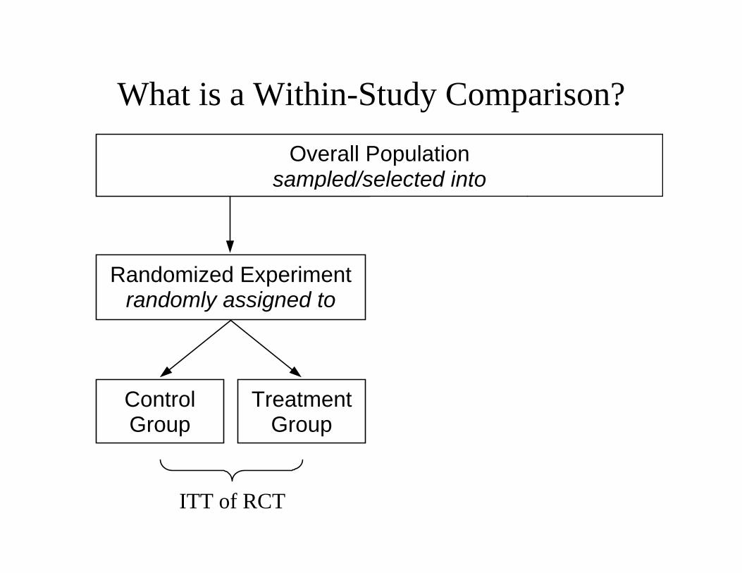
Overall Population sampled/selected into

Randomized Experimentrandomly assigned to

Control Group

TreatmentGroup

Comparison Group

ITT of OSITT of RCT

What is a Within-Study Comparison?

What is a Within-Study Comparison? Overall Population

sampled/selected into


Control Group

TreatmentGroup

Comparison Group

ITT of OSITT of RCT

What is a Within-Study Comparison?

=?

Overall Population sampled/selected into


Control Group

TreatmentGroup

Comparison Group

ITT of OSITT of RCT

Criteria for Comparing Experiments and Q-Es

Clear variation in mode of forming control group--random or notRCT merits being considered a “gold standard’because it demonstrably meets assumptionsExperiment and non-experiment difference is not confounded with 3rd variables like measurementThe quasi-experiment should be a good example of its type--otherwise one compares a good experiment to a poor quasi-experiment

Criteria continued

The experiment and quasi-experiment should estimate the same causal quantity--not LATE vs ATE or ITT vs TOTCriteria for inferring correspondence of results should be clearThe non-experimental analyses should be done blind to the experimental resultsHistorical change in meeting of criteria

Consider 3 examples

Bloom, Michaelopoulos et al.

Aiken, West et al.

Diaz & Handa

Bloom, Michaelopoulos et al

Logic of the design is to compare ES from a randomly created control group with ES from a non-randomly formed comparison that shares the same treatment groupTreatment group is a constant and can be ignored, comparing only the two types of controlIssue is: Will the randomly and non-randomly formed control groups differ over 8 pretest observation points after standard statistical adjustments for any differences in mean or slope

The Context

RCT is on job training at 11 sitesBloom et al restrict the ITS to 5 within-state comparisons, 4 of them within-cityNon-random comparison cases chosen from job training centers in same cityMeasured in the same ways as treated at same times

Results: 3 within-city Samples

What you see in Graphs

Hardly differ at all --- one advantage of TS is that we can see group differencesStatistical tests confirm no differences in intercept or slopeIn these cases, equivalence of randomly and non-randomly formed comparison groups is achieved thru sampling design aloneThus, no need for statistical tests to render them “equivalent”

Two other Sites

Portland--sample size smallest and least stableDetroit vs Grand Rapids--a within-state but not within-

city comparison. Hence, this is not a very local comparison

Bloom et al. Results (2)

Here you see

TS are not equivalent overallTS especially not equivalent around the crucial intervention pointThus use of a random or non-random control group would produce different results10 types of statistical analyses were used to make the series equivalent:

Results of these Analyses

OLS, propensity scores, Heckman selection models, random growth models--all failed to give the same results as the experiment under these conditionsBut the more the pretest time points, the less the biasOnly the random growth model took advantage of the TS nature of the dataWhy did it fail too?

Selecting Intact Groups locally matched on pretest outcomes

Without intending it, Bloom et al’s choice of within-city non-equivalent controls achieved comparability with the randomly formed experimental controls. That is, there was No bias across 3 of the 4 within-city samples; nor for the weighted average of all 4 sitesSo, overlap on observables was achieved through the sampling design alone, precluding need for statistical adjustmentsRemember: There was bias in across-state comparisons, and it could not be adjusted away statistically with the data and models used

Selecting Intact Groups with Maximal Overlap: 2nd Example

Aiken et al. ASU--effects of remedial writingSample selection in their Quasi-Experiment was from the same range of ACTs and SATs as in their experimentDiffered by failure of researchers to contact them over summer and later registrationWhat will the role of unobserved variables be that are correlated with these two features that differentiate randomly and non-randomly formed control units?Measurement framework the same in the experiment and quasi-experiment, as were the intervention and control group experiences

Results

On SAT/CAT, 2 pretest writing measures, the randomly and non-randomly formed comparison groups did not differSo close correspondence on observables w/o any need for statistical adjustment; andIn Q-E, OLS test controls for pretest to add power and not to reduce biasResults for multiple choice writing test in SD units = .59 and .57--both sig. Results for essay = .06 and .16 - both non-sig

3rd Example: Diaz & Handa (2006)

Progresa: Matched Villages with and without the programOne sample of villages had to meet the village eligibility standards--in bottom quintile on test of material resources, but for a variety of reasons not in experimentThe eligible no-treatment comparison families in these villages were not different on outcomes from the randomly created comparison group

But there were different on a few family characteristics

Nonetheless, the results of the matched village analyses were similar whether covariates were added to control for these differences or not

Implications of all Three Studies

Aiken et al and Bloom et al. created non-equivalent control groups that were not different on observables from the treatment group.These observables included a pretest on the same scale as the outcomeDiaz and Handa created much overlap but some differences that did not affect outcomeBut what about unobservables? We never know. But if there are real differences, or real unadjusted differences, then we know to worry

What is a Local, Focal, Non-Equivalent Intact Control Group 1

Local because…Focal because…Non-Equivalent because…Intact because…

What is a Local, Focal, Non-Equivalent Intact Control Group 2

Identical TwinsFraternal TwinsSiblingsSuccessive Grade Cohorts within the same SchoolSame Cohort within different Schools in same DistrictSame Cohort within different Schools in different districts in same stateSame Cohort within different schools in different states, etc.

The Trade Offs here are…

Identity vs. Comparability. We cannot assume that siblings are identical, for example. They have some elements of non-shared genes and environments.Comparability vs. Contamination. Closer they are in terms of space and presumed receptivity to the intervention, the greater the risk of contamination.To reduce an inferential threat is not to prevent it entirely.

Analysis of Workhorse Design Data when group Differences

Modeling the outcome, like covariance analysis

Modeling selection, like Propensity Scores

Empirical Validation literature

Propensity Score Matching

Begin with design of empirical test of propensity score methodsImplementation of a PS analysis1. Causal estimand of interest2. Selection of covariates3. PS estimation4. Estimation of treatment effect5. Sensitivity analysisResults of empirical test

Nonrandomized Experiments (Quasi-Experiments; Observational Studies)A central hypothesis about the use of nonrandomized experiments is that their results can well-approximate results from randomized experiments

especially when the results of the nonrandomized experiment are appropriately adjusted by, for example, selection bias modeling or propensity score analysis. I take the goal of such adjustments to be: to estimate what the effect would have been if the nonrandomly assigned participants had instead been randomly assigned to the same conditions and assessed on the same outcome measures. The latter is a counterfactual that cannot actually be observedSo how is it possible to study whether these adjustments work?

Randomly Assign People to Random or Nonrandom Assigment

One way to test this is to randomly assign participants to being in a randomized or nonrandomized experiment in which they are otherwise treated identically. Then one can adjust the quasi-experimental results to see how well they approximate the randomized results.Here is the design as we implemented it:

Shadish, Clark & Steiner (2008) (Within-Study Comparison)

N = 445 Undergraduate Psychology StudentsRandomly Assigned to

Randomized ExperimentN = 235

Randomly Assigned to

Observational StudyN = 210

Self-Selected into

MathematicsTrainingN = 119

VocabularyTrainingN = 116

MathematicsTrainingN = 79

VocabularyTrainingN = 131

ATE=?

Shadish et al.: Treatments & Outcomes

Two treatments and outcomesTwo treatments: short training either in Vocabulary(advanced vocabulary terms) or Mathematics (exponential equations)→ All participants were treated together without knowledge of the different conditionsTwo outcomes: Vocabulary (30-item posttest) and Mathematics (20-item posttest)

Treatment effect:ATE: average treatment effect for the overall population in the observational study

Shadish et al.: Covariates

Extensive measurement of constructs (in the hope that they would establish strong ignorability):

5 construct domains with 23 constructs based on 156 questionnaire items!

Measured before students were randomly assigned to randomized or quasi-experiment

Hence, measurements are not influenced by assignment or treatment

Shadish et al.: Construct Domains

23 constructs in 5 domainsDemographics (5 single-item constructs): Student‘s age, sex, race (Caucasian, Afro-American, Hispanic), marital status, credit hours

Proxy-pretests (2 multi-item constructs): 36-item Vocabulary Test II, 15-item Arithmetic Aptitude Test

Prior academic achievement (3 multi-item constructs): High school GPA, current college GPA, ACT college admission score

Shadish et al.: Construct Domains

Topic preference (6 multi-item constructs): Liking literature, liking mathematics, preferring mathematics over literature, number of prior mathematics courses, major field of study (math-intensive or not), 25-item mathematics anxiety scale

Psychological predisposition (6 multi-item constructs): Big five personality factors (50 items on extroversion, emotional stability, agreeableness, openness to experience, conscientiousness), Short Beck Depression Inventory (13 items)

Shadish et al.: Unadjusted Results Effects of Math Training on Math Outcome

Math Vocab Mean AbsoluteTng Tng Diff Bias

Mean Mean

Unadjusted Randomized Experiment 11.35 7.16 4.19

Unadjusted Quasi-Experiment 12.38 7.37 5.01 .82

Conclusions: The effect of math training on math scores was larger when participants could self-select into math training.The 4.19 point effect (out of 18 possible points) in the randomized experiment was overestimated by 19.6% (.82 points) in the nonrandomized experiment

Shadish et al.: Unadjusted Results Effects of Vocab Training on Vocab Outcome

Vocab Math Mean AbsoluteTng Tng Diff Bias

Mean Mean

Unadjusted Randomized Experiment 16.19 8.08 8.11

Unadjusted Quasi-Experiment 16.75 7.75 9.00 .89

Conclusions: The effect of vocab training on vocab scores was larger (9 of 30 points) when participants could self-select into vocab training.The 8.11 point effect (out of 30 possible points) in the randomized experiment was overestimated by 11% (.89 points) in the nonrandomized experiment.

Adjusted Quasi-Experiments

It is no surprise that randomized and nonrandomized experiments might yield different answers.The more important question is whether statistical adjustments can improve the quasi-experimental estimate, i.e., remove the selection biasSelection bias can be removed if

The treatment selection is strongly ignorable, i.e., all the covariates that simultaneously affect treatment selection and potential outcome (confounders) are measured

Theory of Strong Ignorability (SI)

If all covariates related to bothtreatment assignment and potential outcomes are observed, and If the selection probabilities, given X, are strictly between zero and one holdsthen, potential outcomes are independent of treatment assignment given observed covariates X:

and treatment assignment is said to be strongly ignorable (strong ignorability; Rosenbaum & Rubin 1983).

X|),( 10 ZYY ⊥

1)|1(0 <=< XZP

),,( 1 ′= pXX KX

Practice of Strong Ignorability (SI)

Need to measure all confounding covariates! If not all covariates, that are simultaneously related to treatment selection and potential outcomes, are observed

the strong ignorability assumption is not met and the average treatment effect will remain biased!

Need to measure covariates reliably (with respect to the selection mechanism)Each subject must have a positive probability of being in the treatment group (overlap).

How to Estimate an Unbiased Treatment Effect?

Assume that we observe all covariates X such that SI holds, then selection bias can be removed with different approaches With original covariates X

Covariance adjustments (standard regression methods)Case matching on observed covariatesMultivariate stratification

With a composite of original covariates b = f(X)Propensity scores (Rosenbaum & Rubin, 1983)Other approaches we will not consider: first discriminant, prognosis scores

Propensity Scores (PS)

The propensity score is the conditional probability that a subject belongs to the treatment group given the observed covariates X:

If treatment selection is strongly ignorable given an observed set of individual covariates X, then it is also strongly ignorable when these individual covariates are combined into a propensity score e(X), i.e.

with(proved Rosenbaum & Rubin 1983)

)|1()( XX == ZPe

)(|),( 10 XeZYY ⊥ 1)(0 << Xe

Propensity Scores (PS)

The propensity score reduces all the information in the predictors to one number

This can make it easier to do matching or stratifying when there are multiple matching variables available.

In a randomized experiment, the true propensity score is .50 for each personIn a quasi-experiment, the true propensity score is unknown

Estimated Propensity Scores

PS needs to be estimated from observed data, e.g., using logistic regression

Weighted composite of all covariates affecting treatment selection (covariates that do not affect selection are typically not included in the PS model)Estimated PS is used to match treatment and control cases with the same or very similar values Therefore, the matched treatment and comparison group are equivalent on the PS (as it would be in a RCT)Interpretation: if treatment = 1 and control = 0, then a propensity score closer to 1.00 (e.g., .83) is a prediction that the person is more likely to be in the treatment group

Example (treatment, covariates, PS)

Steps in Conducting a PS Analysis

Steps in conducting a PS analysis1. Choice of the treatment effect of interest2. Assessing strong ignorability3. Estimation of the PS4. Estimation of the treatment effect & standard errors5. Sensitivity analysis

Use data from Shadish et al. (2008) to illustrate

PS Analysis


Choice of Treatment effect

Types of treatment effects:Average treatment effect (ATE):Treatment effect for the overall target population in the study (treated and untreated subjects together)Average treatment effect for the treated (ATT):Treatment effect for the treated subjects onlyAverage treatment effect for the untreated (ATU):Treatment effect for the untreated subjects only

ATE, ATT, and ATU differ if the treatment effect is not constant (heterogeneous) across subjects

Choice of Treatment effect

Choice depends on the research question (and sometimes on the data at hand)Example: Effect of retaining students on achievement scores (one or more years after retaining):

ATT investigates the effect of retaining on the retained students (What would have happened if the retained students would have not been retained?)ATE investigates the effect of retaining if all students would have been retained vs. all would have passed

Shadish et al.: ATEWhat is the treatment effect if all students would have received the vocabulary (math) training?

PS Analysis


Assessing Covariates & SI

If a causal treatment effect should be estimated, we need to assess whether strong ignorability holds

Are at least all constructs that simultaneously affect treatment selection and potential outcomes measured?If selection is on latent constructs (e.g., self-selection dependent on ability) instead of observed ones (e.g., administrator selection on reported achievement scores), are those constructs reliably measured?

If some important covariates are missing or highly unreliable causal claims are probably not warranted!

Hidden bias, i.e., bias due to unobserved covariates, may remain.


How can we guess that SI holds?Strong theories on selection process and outcome modelExpert knowledgeDirect investigation of the selection processHaving a large number of covariates from heterogeneous domains

Are there groups of covariates that justify SI more than others?

Pretest measures on the outcome do usually betterDirect measures of the selection processEasily available data like demographic are typically not sufficient for warranting SI!


Shadish et al. (2008):Extensive & reliable measurement of different construct domains and constructs

Pretest measures, though only proxy-pretest measures (assumed to be highly correlated with potential outcomes)Direct measures of the assumed selection process, e.g., like mathematics, prefer literature over math (assumed to be highly correlated with the selection process)Broad range of other measures on prior academic achievement, demographics, psychological predisposition

Would we have been confident in assuming SI—without having our experimental benchmark?

PS Analysis


Estimation of PS

Different methods for estimating PS can be used:Binomial models: logistic regression, probit regression

• Most widely used• Rely on functional form assumption

Statistical learning algorithms (data mining methods):classification trees, boosting, bagging, random forests

• Do not rely on functional form assumptions• It is not yet clear, whether these methods are on average

better than binomial models

Estimation of PS

Logistic regression of treatment Z on observed predictors W (covariates X or transformations thereof, e.g. polynomials, log, interactions)

Logistic model:Estimated PS logit:Estimated PS :

PS (logit) is the predicted value from the logistic regression

The distribution of the estimated PS-logit shows how similar/different treatment and control group are

γW~)(logit Zγˆ W=l

)ˆexp(1)ˆexp(el

l+

=

Sample SPSS Syntax

LOGISTIC REGRESSION VAR=vm/METHOD=ENTER vocabpre numbma_r likema_r likeli_r prefli_r pextra pconsc

beck cauc afram age momdeg_r daddeg_r majormi liked avoided selfimpr

/SAVE PRED (ps).

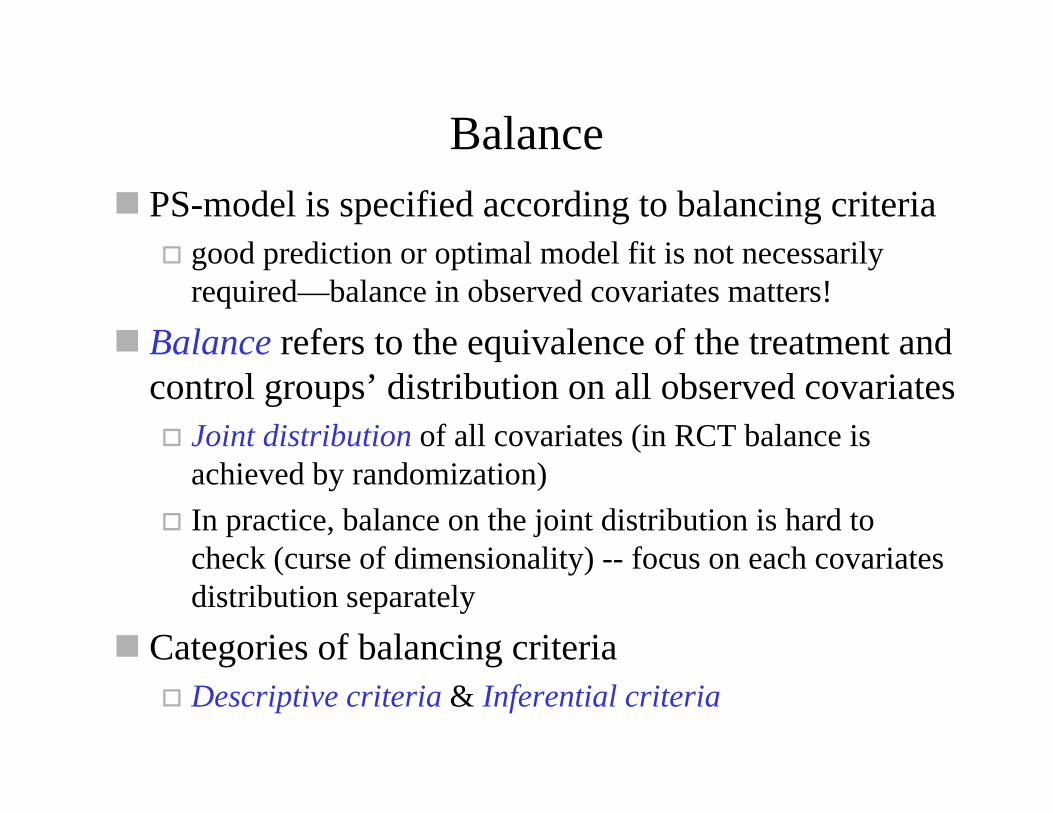
BalancePS-model is specified according to balancing criteria

good prediction or optimal model fit is not necessarily required—balance in observed covariates matters!

Balance refers to the equivalence of the treatment and control groups’ distribution on all observed covariates

Joint distribution of all covariates (in RCT balance is achieved by randomization)In practice, balance on the joint distribution is hard to check (curse of dimensionality) -- focus on each covariates distribution separately

Categories of balancing criteriaDescriptive criteria & Inferential criteria

Balance

Descriptive criteria that compare the covariate distribution of the treatment and control group beforeand after PS-adjustment:

Visual inspection: Comparison of histograms or kernel density estimates; QQ-plots

Initial Imbalance before PS adjust. (Shadish et al., 2008)

0 10 20 30

vocabpre

p(F): 0.014 p(KS): 0.097

0 5 10 15

mathpre

p(F): 0.193 p(KS): 0.569

0 1

afram

p(logit): 0.038 p(chisq): 0.052

0 2 4 6 8 10 12

likemath

p(F): 0.000 p(KS): 0.000

0 2 4 6 8 10 12

likelit

p(F): 0.017 p(KS): 0.037

1 2 3

preflit

p(F): 0.000 p(KS): 0.000

Balance after PS-Adjustment

0 10 20 30

vocabpre

M/IA: 0.970 / 0.984 Mwt: 0.939

0 5 10 15

mathpre

M/IA: 0.887 / 0.595 Mwt: 0.727

0 1

afram

M/IA: 0.915 / 0.150 Mwt: 0.884

0 2 4 6 8 10 12

likemath

M/IA: 0.883 / 0.585 Mwt: 0.829

0 2 4 6 8 10 12

likelit

M/IA: 0.855 / 0.202 Mwt: 0.968

1 2 3

preflit

M/IA: 0.544 / 0.618 Mwt: 0.805

Balance

Descriptive criteria that compare the covariate distribution of the treatment and control group:

Visual inspection: Comparison of histograms or kernel density estimates; QQ-plotsStandardized mean difference & variance ratio (Rubin, 2001)

• Standardized mean difference (Cohen’s d)

d should be close to zero (|d| < 0.1)• Variance ratioν should be close to one (4/5 < ν < 5/4)

• Can also be applied to PS-strata separately for checking balance at different regions of the PS distribution

2/)(/)( 22ctct ssxxd +−=

22 / ct ssv =

-1.0 -0.5 0.0 0.5 1.0

0.5

1.0

1.5

2.0

standardized difference in means

varia

nce

ratio

+

collgpaa

lnumbmath

pextra

balance after PS-adjustment

(Im)balance in Covariates and PS-logit (23 covariates)

-1.0 -0.5 0.0 0.5 1.0

0.5

1.0

1.5

2.0

standardized difference in means

varia

nce

ratio

+

male afram mathpre

collgpaa likemath lnumbmath

majormi

pconsc

cauc

vocabpre

likelit

preflit

mars

pextra pagree

pintell

initial imbalance

Balance

Inferential criteria that compare the covariate distribution of the treatment and control group:

t-test comparing group meansHotelling’s T (multiviariate version of t-test)Kolmogorov-Smirnov test comparing distributionsRegression tests

(Dis)advantage of inferential criteria:Depend on sample size

• No enough power for small samples• Hard to achieve balance for large samples

Overlap & Balance (PS-logit)

-3 -2 -1 0 1 2 3

Propensity Score Logits (by quintiles)

MathematicsVocabulary

before PS-adjustment

-4 -2 0 2 4

Propensity Score Logits

MathematicsVocabulary

after PS-adjustment

Overlap

Overlap of groups: the treatment and control group’s common support region on the PS(-logit)

For non-overlapping cases the treatment effect cannot be estimatedNon-overlapping cases might be the reason why balance cannot be achieved

• Balance should be checked after deletion of non-overlapping cases

Discarding non-overlapping cases restricts the generalizability of results

• Discarding on the basis of covariate values instead of PS retains the interpretability of the treatment effect

Overlap

Example (simulation)

How to Specify a PS Model

1. Estimate a good fitting logistic regression by Including higher-order terms and interaction effects of covariates (also try transformed covariate, e.g., log)Using usual fitting criteria, e.g. AIC or log-likelihood test

2. Delete non-overlapping cases3. Check balance using the same PS techniques as is

later used for estimating the treatment effect4. If balance is not satisfying re-specify PS model (on

all cases) by including further covariates, higher-order terms or interaction effects

5. Go to 2, repeat until satisfactory balance is achieved

What if Balance/Overlap cannot be achieved?

Indication that groups are too heterogeneous for estimating a causal treatment effect (particularly if groups only overlap on their tails)If imbalance is not too severe one could hope that the additional covariance adjustment removes the residual bias due to imperfect balanceIt is usually harder to achieve balance on a large set of covariates than on small set of covariates

PS Analysis

Steps in conducting a PS analysis1. Choice of the treatment effect of interest2. Assessing strong ignorability3. Estimation of the PS4. Estimation of the treatment effect & standard

errors5. Sensitivity analysis

Choice of PS technique

Four groups of PS techniques (Schafer & Kang, 2008; Morgan & Winship, 2007:

Individual case matching on PSPS-StratificationInverse PS-WeightingRegression estimation (ANCOVA) using PS

Combination with an additional covariance adjustment (within the regression framework)

Makes estimates “doubly robust”, i.e., robust against the misspecification either of the PS model or outcome modelHowever, if both models are misspecified, bias can also increase (Kang & Schafer, 2007)

Individual Case Matching

General idea: for each treated subject find at least one control subject who has the same or a very similar PS

Matching estimators typically estimate ATT

Types of matching strategies/algorithmsNumber of matches: 1:1 matching, 1:k matching, full matchingReplacement: With or without replacement of previously matched subjectsSimilarity of matches: Exact matching, caliper matchingAlgorithm: Optimal matching, genetic matching, greedy matching, ...


Standard matching procedures results in two groups:Matched treatment group (might be smaller than the original treatment group if no adequate matches were found) Matched control group (those cases of the original control group that where matched to one or more treatment cases)

Estimation of the treatment effect:Difference in the treatment and control means of the matched samples, (one- or two sample t-test) Alternatively, using regression without or with additional covariance adjustment:

01ˆ mm YY −=τ

mm ZY τα ˆˆˆ += βτα ˆˆˆˆmmm ZY X++=


Matching procedures are available in different statistical (programming) packages:

R: MatchIt (Ho, Imai, King & Stuart, in print) Matching (Sekhon, in print)optmatch (Hansen & Klopfer, 2006)

STATA: PSMATCH2 (Leuven & Sianesi, 2003) MATCH (Abadie et al., 2004) PSCORE (Becker & Ichino, 2002)

SAS: greedy matching (Parsons, 2001) optimal matching (Kosanke & Bergstralh, 2004 )

SPSS: greedy matching (Levesque R. Raynald’s SPSSTools)

PS-Stratification

Use the PS to stratify all observations into j = 1, …, kstrata

Most frequently quantiles are usedQuantiles: remove approx. 90% of the bias (given SI holds)More strata remove more bias but the number of treated and control cases should not be too small (> 10 obs.)

Estimate the treatment effect within each stratummean difference within each stratum oradditional covariance adjustment removes residual bias: regression within each k strata:

jjj YY 01ˆ −=τ

jjjjjj ZY βτα ˆˆˆˆ X++=

PS-Stratification

Pool the stratum-specific treatment effects

with weightsfor ATEfor ATT

Standard error: pooled stratum-specific standard errors

∑=

=k

jjj w

1

ˆˆ ττ

nnnw jjj )( 10 +=.11 nnw jj =

Stratum j = 1 j = 2 … j = k sumZ = 0 n01 n02 … n0k n0.

Z = 1 n11 n12 … n1k n1.

sum n.1 n.2 … n.k n ATEATT

PS-Stratification Example(Shadish et al.)

-3 -2 -1 0 1 2 3

05

1015

Mathematics

PS-logit

Mat

hem

atic

s Sc

ore

PS-StratificationShadish et al. (2008): Mathematics outcome

Stratum-specific means and treatment effect & ATE

Sample size and ATE-weightsStratum j = 1 j = 2 … j = k sumZ = 0 7 24 29 34 37 131Z = 1 35 18 13 8 5 79sum 42 42 42 42 42 210weights .2 .2 .2 .2 .2 1

means j = 1 j = 2 j = 3 j = 4 j = 5 meanZ = 0 12.9 8.0 8.2 6.5 6.0 8.3Z = 1 13.0 12.3 10.9 12.8 11.2 12.0

0.1 4.2 2.7 6.3 5.2 3.7τ ATE

ATE

PS-StratificationStratum-specific means and treatment effect & ATT

= .1·.44 + 4.2·.23 + 2.7·.16 + 6.3·.10 + 5.2·.06 = 2.4Sample size and ATT-weights

Stratum j = 1 j = 2 … j = k sumZ = 0 7 24 29 34 37 131Z = 1 35 18 13 8 5 79sum 42 42 42 42 42 210weights .44 .23 .16 .10 .06 1

means j = 1 j = 2 j = 3 j = 4 j = 5 meanZ = 0 12.9 8.0 8.2 6.5 6.0 8.3Z = 1 13.0 12.3 10.9 12.8 11.2 12.0

0.1 4.2 2.7 6.3 5.2 2.4τ ATT

ATT

τ

Inverse PS-Weighting

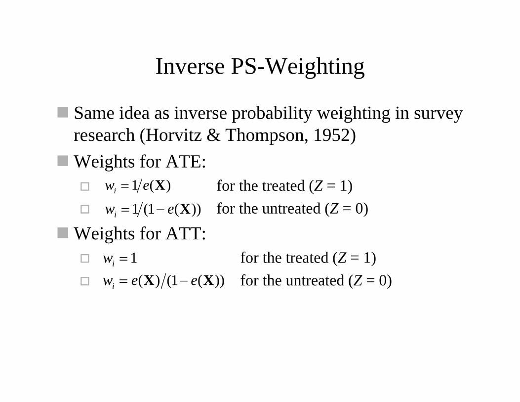
Same idea as inverse probability weighting in survey research (Horvitz & Thompson, 1952)Weights for ATE:

for the treated (Z = 1)for the untreated (Z = 0)

Weights for ATT:for the treated (Z = 1)for the untreated (Z = 0)

)(1 Xewi =

))(1(1 Xewi −=

))(1()( XX eewi −=1=iw

Inverse PS-Weighting

Treatment effect:Treatment effect is the difference between the weighted treatment and control means, which can also be estimated usingWeighted least squares regression (WLS) without or with covariates

Disadvantage:Sensitivity to large weightsLarger standard errors

Regression Estimation using PS

PS can be included as additional covariate in standard regression approaches. The PS can be included as

Quadratic or cubic polynomial of PS or PS-logit (the latter is more likely linearly related to the outcome)Dummy variables for PS strata like deciles, for instance. Is less restrictive than the polynomial.Combination of dummy variables and the linear PS-logit

As simple regression estimate can be obtained by using the cubic polynomial of the PS logit, for instance,

strong functional form assumptions (same from for T & C)ATE or ATT is not clearly defined

γβββτα ˆˆˆˆˆˆˆˆˆˆ 33

221 X+++++= lllZY

Regression Estimation using PS

A better approach is as follows (regression estimation; Schafer & Kang, 2008):

Estimate the regression model for each group separatelyUse the estimated treatment regression for predicting the missing treatment outcomes of the control groupUse the estimated control regression for predicting the missing control outcomes of the treatment groupCompute for each subject the difference between the observed (predicted) treatment and predicted (observed) control outcomeThe average across these differences estimates ATE

ATE & Bias Reduction: Vocabulary

Vocabulary Outcome

Mean Diff. (s.e.) R2 Percent Bias

Reduction Covariate-Adjusted Randomized Exp. 8.25 (.37) .71 Unadjusted Quasi-Experiment 9.00 (.51) .60 PS Stratification 8.11 (.52) .76 80% PS Linear ANCOVA 8.07 (.47) .76 76% PS Nonlinear ANCOVA 8.03 (.48) .77 70% PS Weighting 8.19 (.51) .76 91% PS Stratification (Pred. of Convenience) 8.68 (.47) .65 43% ANCOVA Using Observed Covariates 8.21 (.43) .76 94%

ATE & Bias Reduction: Mathematics

Mathematics Outcome

Mean Diff. (s.e.) R2 Percent Bias

Reduction Covariate-Adjusted Randomized Exp. 4.01 (.35) .58 Unadjusted Quasi-Experiment 5.01 (.55) .28 PS Stratification 3.74 (.42) .66 73% PS Linear ANCOVA 3.65 (.42) .64 64% PS Nonlinear ANCOVA 3.67 (.42) .63 66% PS Weighting 3.71 (.40) .66 70% PS Stratification (Pred. of Convenience) 5.06 (.51) .35 -5% ANCOVA Using Observed Covariates 3.85 (.44) .63 84%

Structural Equation Models as Adjustments

If ordinary ANCOVA did well, perhaps SEM would do well too.After all, it can do more complex models than ordinary ANCOVA:

Which Method Should be Chosen?

BiasWithout additional covariance adjustment matching and stratification results in some residual bias (due to inexact matching)Regression estimation relies on functional form assumptions

EfficiencySome matching estimator are sometimes less efficient because not all available observations are used (except for optimal full matching)Weighting estimators are less efficient (due to extreme weights)


Sample Size RequirementsMatching does better with large samples and a considerably larger number of control cases than treatment casesIn general, PS methods are a large sample technique

Treatment effectMatching is better suited for estimating ATTAll other methods handle ATT and ATE equally well

Ease of ImplementationMatching requires special software tools, but they are available in most major statistical software packagesOther methods are easy to implement (except s.e. estimation)


Additional covariance adjustmentShould be done, though it might sometimes introduce additional biasWith an additional covariate adjustment, the difference between PS methods gets smaller

Does the choice of specific technique make a difference?

In general, differences are smallHowever, for specific data sets it might make a difference

PS Analysis


Sensitivity Analysis

How sensitive is the estimated treatment effect to unobserved confounders?

Need to assume how strongly such an unobserved covariate is correlated with treatment selection and potential outcomes

• assume that the unobserved covariate is as strongly correlated with treatment and outcome as the (second) most important observed covariate

• Sensitivity is determined using a regression approachAlternatively one can ask how strongly a covariate has to be correlated with treatment and outcome such that the treatment effect is no longer different from zero

Empirical Test of PS

Relative Importance ofCovariate selectionReliable measurementChoice of analytic methods

Relative Importance

What are the most important factors for establishing SI and getting an unbiased causal estimate?

Selection of constructs related to both treatment selection and potential outcomesReliable measurement of constructsBalancing pre-treatment baseline differences(i.e., correct specification of PS model)Choice of the analytic method(PS methods or ANCOVA)

Ruling out hidden bias

Avoiding overt bias

Importance of Covariate SelectionSteiner, Cook, Shadish & Clark (2011)

Investigate the importance ofConstruct domainsSingle constructs

for establishing strong ignorabilityCompare it to the importance of choosing a specific analytic method

Bias Reduction: Construct DomainsVocabulary

1

11 1 1 1

11

11

1

11

1 1 1

-20

0

20

40

60

80

100

120

140

Bia

s R

educ

tion

(%)

22 2

2

2

22 2 2

22

2

2

22 2

3 3 3

3 3

3

33

33

33 3 3 3

3

4 4

4

4 4

44

4 44 4

4

4

4

4 4

1234

PS-stratificationPS-ANCOVAPS-weightingANCOVA

1

11 1 1 1

11

11

1

11

1 1 1

22 2

2

2

22 2 2

22

2

2

22 2

3 3 3

3 3

3

33

33

33 3 3 3

3

4 4

4

4 4

44

4 44 4

4

4

4

4 4

psy aca dem pre top dempsy

demaca

dempre

prepsy

demtop

preaca

pretop

dempreaca

dempretop

dempreacatop

dempreacatoppsy

psy aca dem

1

11 1 1 1

11

11

1

11

1 1 1

-20

0

20

40

60

80

100

120

140

Bia

s R

educ

tion

(%)

22 2

2

2

22 2 2

22

2

2

22 2

3 3 3

3 3

3

33

33

33 3 3 3

3

4 4

4

4 4

44

4 44 4

4

4

4

4 4

1234

PS-stratificationPS-ANCOVAPS-weightingANCOVA

1

11 1 1 1

11

11

1

11

1 1 1

22 2

2

2

22 2 2

22

2

2

22 2

3 3 3

3 3

3

33

33

33 3 3 3

3

4 4

4

4 4

44

4 44 4

4

4

4

4 4

psy aca dem pre top dempsy

demaca

dempre

prepsy

demtop

preaca

pretop

dempreaca

dempretop

dempreacatop

dempreacatoppsy

psy aca dem

Bias Reduction: Construct DomainsVocabulary

Bias Reduction: Construct DomainsMathematics

11

1

1

1

1

1

1

11

1 1

1

1

1

1

-20

0

20

40

60

80

100

120

140

Bia

s R

educ

tion

(%)

2

2

22

2

2

2

2 2

2

2 2

2

2

2

2

3

33

3

3

3

3 3 33

33

3

3

3

3

4

44

4

4

4

4 4 4

4

4 4

4

44 4

1234

PS-stratificationPS-ANCOVAPS-weightingANCOVA1

1

1

1

1

1

1

1

11

1 1

1

1

1

1

2

2

22

2

2

2

2 2

2

2 2

2

2

2

2

3

33

3

3

3

3 3 33

33

3

3

3

3

4

44

4

4

4

4 4 4

4

4 4

4

44 4

psy dem aca pre top dempsy

prepsy

demaca

dempre

preaca

demtop

pretop

dempreaca

dempretop

dempreacatop

dempreacatoppsy

psy dem aca

Bias Reduction: Single ConstructsVocabulary

1

1

11

11

1

1

1 1

11

-40

-20

0

20

40

60

80

100

120

140

Bia

s R

educ

tion

(%)

2

2

22

22

2

2 22 2

2

3

3

33

3

3 3

33 3 3

3

4

4

4

44 4

4

4

4

4

4

4

1234


1

11

11

1

1

1 1

11

2

2

22

22

2

2 22 2

2

3

3

33

3

3 3

33 3 3

3

4

4

4

44 4

4

4

4

4

4

4

proxy-pretest topic preference all covariates except

mat

h.pr

e

voca

b.pr

e

num

bmat

h

mar

s

maj

or

like.

mat

h

like.

lit

pref

.mat

h

-voc

ab.p

re-p

ref.m

ath

-voc

ab.p

re

-pre

f.mat

h all

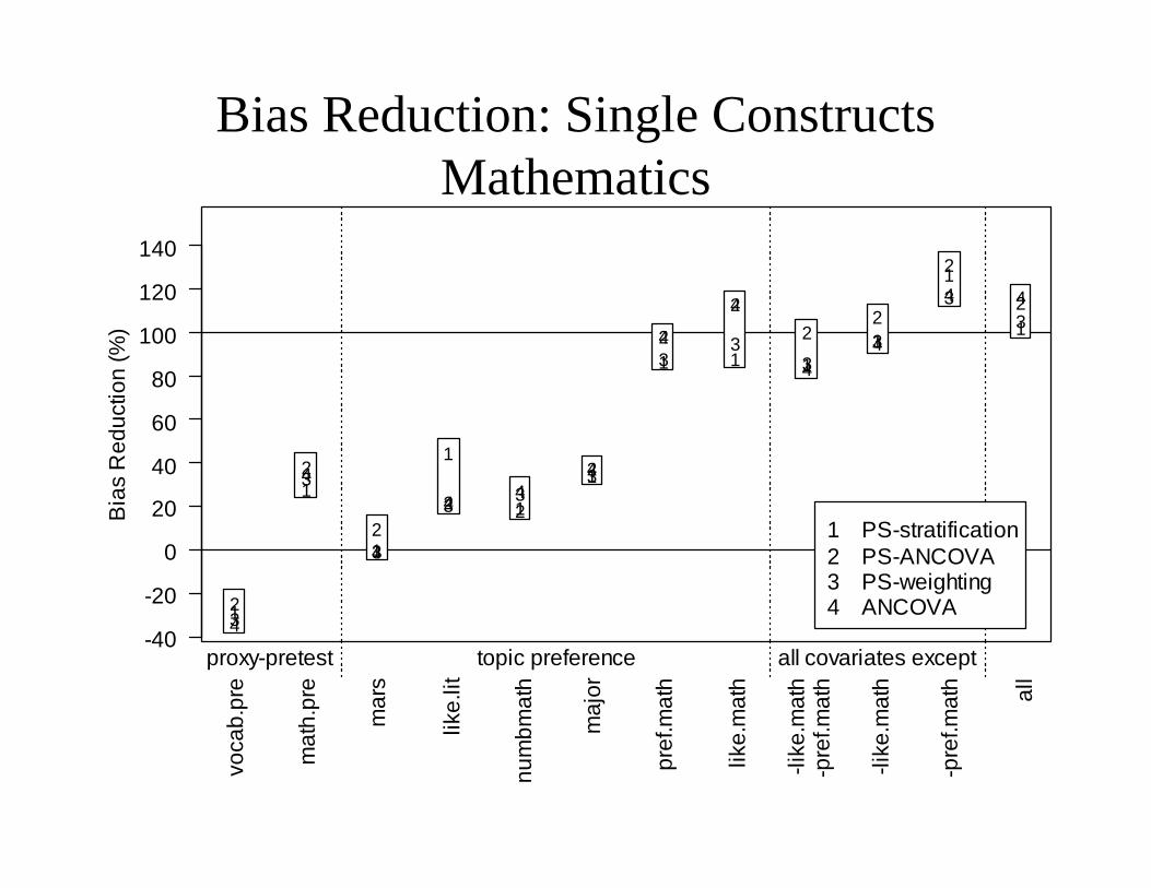
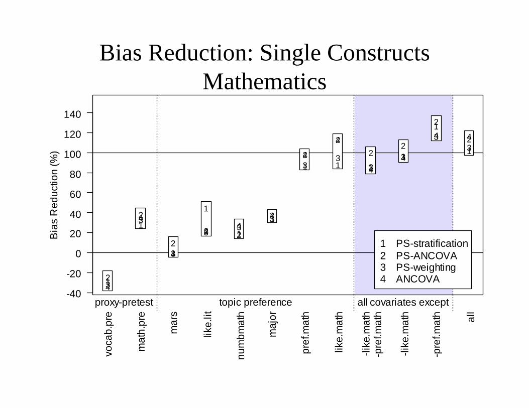
Bias Reduction: Single ConstructsMathematics

1

1

1

1

1

1

1 1 11

1

1

-40

-20

0

20

40

60

80

100

120

140

Bia

s R

educ

tion

(%)

2

2

22 2

2

2

22

2

2

2

3

3

3

3 33

33

33

33

4

4

4

4 44

4

4

44

4 4

1234


1

1

1

1

1

1 1 11

1

1

2

2

22 2

2

2

22

2

2

2

3

3

3

3 33

33

33

33

4

4

4

4 44

4

4

44

4 4

proxy-pretest topic preference all covariates except

voca

b.pr

e

mat

h.pr

e

mar

s

like.

lit

num

bmat

h

maj

or

pref

.mat

h

like.

mat

h

-lik

e.m

ath

-pre

f.mat

h

-lik

e.m

ath

-pre

f.mat

h all

Constructs: Conclusion

In establishing SI selection of constructs matters Need those construct domains that effectively reduce bias (those related to both treatment selection and outcome)Need the right single constructs within domains because only a few covariates successfully reduce bias

Choice of analytic method is less important (given its competent implementation)

No systematic difference between PS methodsANCOVA did as well (at least in that case)

Reliability of Construct MeasurementSteiner, Cook & Shadish (in press)

How important is the reliable measurement of constructs (given selection on latent constructs)?

Does the inclusion of a large set of covariates in the PS model compensate for each covariate‘s unreliable measurement?

Add measurement error to the observed covariates in a simulation study

Assume that original set of covariates is measured without error and removes 100% of selection biasSystematically added measurement error such that the reliability of each covariate was ρ =.5, .6, .7, .8, .9, 1.0

Vocabulary: Reliability 1.0

1

1

1

11

1

11

1

1

1-40

-20

0

20

40

60

80

100

120

Bia

s R

educ

tion

(%)

2

2

2

2 22

22

2

2

2

3

3

3

3

3 3

33

3

3

3

4

44

4

4 4

44

4

4

4

1234

PS-stratificat.PS-ANCOVAPS-weightingANCOVA

1

1

1

11

1

2

2

2

2 22

3

3

3

3

3 3

4

44

4

4 4

4

44

4

4 4

44

4

4

4

all top pre dem aca psy vocabpre

prefmath

likelit

likemath

mathpre

1

1

1

11

1

2

2

2

2 22

3

3

3

3

3 3

4

44

4

4 4

44

4

4

4

Vocabulary: Reliability .9

1

1

1

11

1

11

1

1

1-40

-20

0

20

40

60

80

100

120

Bia

s R

educ

tion

(%)

2

2

2

2 22

22

2

2

2

3

3

3

3

3 3

33

3

3

3

4

44

4

4 4

44

4

4

4

1234


1

1

1

11

1

2

2

2

2 22

3

3

3

3

3 3

4

44

4

4 4

4

44

4

4 4

44

4

4

4


prefmath

likelit

likemath

mathpre

1

1

1

11

1

2

2

2

2 22

3

3

3

3

3 3

4

44

4

4 4

44

4

4

4

1

1

1

1

1 1

2

2

2

22 2

3

3

33

3 3

4

44

4

4 4

4 4

4

4

4


1

1

1

11

1

11

1

1

1-40

-20

0

20

40

60

80

100

120

Bia

s R

educ

tion

(%)

2

2

2

2 22

22

2

2

2

3

3

3

3

3 3

33

3

3

3

4

44

4

4 4

44

4

4

4

1234


1

1

1

11

1

2

2

2

2 22

3

3

3

3

3 3

4

44

4

4 4

4

44

4

4 4

44

4

4

4


prefmath

likelit

likemath

mathpre

1

1

1

11

1

2

2

2

2 22

3

3

3

3

3 3

4

44

4

4 4

44

4

4

4

1

1

1

1

1 1

2

2

2

22 2

3

3

33

3 3

4

44

4

4 4

4 4

4

4

4

1

1

11

1 1

2

2

2

2

2 2

3

3

3 3

3 3

4

44 4

4 4

4 4

44

4


1

1

1

11

1

11

1

1

1-40

-20

0

20

40

60

80

100

120

Bia

s R

educ

tion

(%)

2

2

2

2 22

22

2

2

2

3

3

3

3

3 3

33

3

3

3

4

44

4

4 4

44

4

4

4

1234


1

1

1

11

1

2

2

2

2 22

3

3

3

3

3 3

4

44

4

4 4

4

44

4

4 4

44

4

4

4


prefmath

likelit

likemath

mathpre

1

1

1

11

1

2

2

2

2 22

3

3

3

3

3 3

4

44

4

4 4

44

4

4

4

1

1

1

1

1 1

2

2

2

22 2

3

3

33

3 3

4

44

4

4 4

4 4

4

4

4

1

1

11

1 1

2

2

2

2

2 2

3

3

3 3

3 3

4

44 4

4 4

4 4

44

4

1

1

1 1

1 1

2

2

22

2 2

3

3

33

3 3

4

44 4

4 4

4 4

44

4


1

1

1

11

1

11

1

1

1-40

-20

0

20

40

60

80

100

120

Bia

s R

educ

tion

(%)

2

2

2

2 22

22

2

2

2

3

3

3

3

3 3

33

3

3

3

4

44

4

4 4

44

4

4

4

1234


1

1

1

11

1

2

2

2

2 22

3

3

3

3

3 3

4

44

4

4 4

4

44

4

4 4

44

4

4

4


prefmath

likelit

likemath

mathpre

1

1

1

11

1

2

2

2

2 22

3

3

3

3

3 3

4

44

4

4 4

44

4

4

4

1

1

1

1

1 1

2

2

2

22 2

3

3

33

3 3

4

44

4

4 4

4 4

4

4

4

1

1

11

1 1

2

2

2

2

2 2

3

3

3 3

3 3

4

44 4

4 4

4 4

44

4

1

1

1 1

1 1

2

2

22

2 2

3

3

33

3 3

4

44 4

4 4

4 4

44

4

1

1

1 1

1 1

2

2

2 2

2 2

3

3

33

3 3

4

44

4

4 4

4 4

44

4


1

1

1

11

1

11

1

1

1-40

-20

0

20

40

60

80

100

120

Bia

s R

educ

tion

(%)

2

2

2

2 22

22

2

2

2

3

3

3

3

3 3

33

3

3

3

4

44

4

4 4

44

4

4

4

1234


1

1

1

11

1

2

2

2

2 22

3

3

3

3

3 3

4

44

4

4 4

4

44

4

4 4

44

4

4

4


prefmath

likelit

likemath

mathpre

1

1

1

11

1

2

2

2

2 22

3

3

3

3

3 3

4

44

4

4 4

44

4

4

4

1

1

1

1

1 1

2

2

2

22 2

3

3

33

3 3

4

44

4

4 4

4 4

4

4

4

1

1

11

1 1

2

2

2

2

2 2

3

3

3 3

3 3

4

44 4

4 4

4 4

44

4

1

1

1 1

1 1

2

2

22

2 2

3

3

33

3 3

4

44 4

4 4

4 4

44

4

1

1

1 1

1 1

2

2

2 2

2 2

3

3

33

3 3

4

44

4

4 4

4 4

44

4

1

1

11

11

2

2

2 2

22

3

3

3

3

33

4

44

4

4 4

4 4

44

4

Mathematics: Reliability 1.0

11

1

1 1 1

11

11

1-40

-20

0

20

40

60

80

100

120

Bia

s R

educ

tion

(%)

22

2

22 2

22

22

2

3 3

3

33 3

33

33

3

44

4

4 4 4

44

44

4

1234


11

1

1 1 1

22

2

22 2

3 3

3

33 3

44

4

4 4 4

44

4

4 4 4

44

44

4

all top pre dem aca psy likemath

prefmath

mathpre

likelit

vocabpre

11

1

1 1 1

22

2

22 2

3 3

3

33 3

44

4

4 4 4

44

44

4

Mathematics: Reliability .9

11

1

1 1 1

11

11

1-40

-20

0

20

40

60

80

100

120

Bia

s R

educ

tion

(%)

22

2

22 2

22

22

2

3 3

3

33 3

33

33

3

44

4

4 4 4

44

44

4

1234


11

1

1 1 1

22

2

22 2

3 3

3

33 3

44

4

4 4 4

44

4

4 4 4

44

44

4


prefmath

mathpre

likelit

vocabpre

11

1

1 1 1

22

2

22 2

3 3

3

33 3

44

4

4 4 4

44

44

4

1 1

1

1 11

22

22

22

3 3

3

33 3

44

44 4

4

44

44

4


11

1

1 1 1

11

11

1-40

-20

0

20

40

60

80

100

120

Bia

s R

educ

tion

(%)

22

2

22 2

22

22

2

3 3

3

33 3

33

33

3

44

4

4 4 4

44

44

4

1234


11

1

1 1 1

22

2

22 2

3 3

3

33 3

44

4

4 4 4

44

4

4 4 4

44

44

4


prefmath

mathpre

likelit

vocabpre

11

1

1 1 1

22

2

22 2

3 3

3

33 3

44

4

4 4 4

44

44

4

1 1

1

1 11

22

22

22

3 3

3

33 3

44

44 4

4

44

44

4

1 1

11 1

1

22

2 22 2

3 3

33

3 3

44

44 4 4

44

44

4


11

1

1 1 1

11

11

1-40

-20

0

20

40

60

80

100

120

Bia

s R

educ

tion

(%)

22

2

22 2

22

22

2

3 3

3

33 3

33

33

3

44

4

4 4 4

44

44

4

1234


11

1

1 1 1

22

2

22 2

3 3

3

33 3

44

4

4 4 4

44

4

4 4 4

44

44

4


prefmath

mathpre

likelit

vocabpre

11

1

1 1 1

22

2

22 2

3 3

3

33 3

44

4

4 4 4

44

44

4

1 1

1

1 11

22

22

22

3 3

3

33 3

44

44 4

4

44

44

4

1 1

11 1

1

22

2 22 2

3 3

33

3 3

44

44 4 4

44

44

4

1 1

11 1

1

22

2 22

2

3 3

3 33 3

44

4 4 4 4

44

44

4


11

1

1 1 1

11

11

1-40

-20

0

20

40

60

80

100

120

Bia

s R

educ

tion

(%)

22

2

22 2

22

22

2

3 3

3

33 3

33

33

3

44

4

4 4 4

44

44

4

1234


11

1

1 1 1

22

2

22 2

3 3

3

33 3

44

4

4 4 4

44

4

4 4 4

44

44

4


prefmath

mathpre

likelit

vocabpre

11

1

1 1 1

22

2

22 2

3 3

3

33 3

44

4

4 4 4

44

44

4

1 1

1

1 11

22

22

22

3 3

3

33 3

44

44 4

4

44

44

4

1 1

11 1

1

22

2 22 2

3 3

33

3 3

44

44 4 4

44

44

4

1 1

11 1

1

22

2 22

2

3 3

3 33 3

44

4 4 4 4

44

44

4

1 1

1 1 1 1

22

2 22 2

3 3

3 33 3

44

4 4 4 4

44

4 4

4


11

1

1 1 1

11

11

1-40

-20

0

20

40

60

80

100

120

Bia

s R

educ

tion

(%)

22

2

22 2

22

22

2

3 3

3

33 3

33

33

3

44

4

4 4 4

44

44

4

1234


11

1

1 1 1

22

2

22 2

3 3

3

33 3

44

4

4 4 4

44

4

4 4 4

44

44

4


prefmath

mathpre

likelit

vocabpre

11

1

1 1 1

22

2

22 2

3 3

3

33 3

44

4

4 4 4

44

44

4

1 1

1

1 11

22

22

22

3 3

3

33 3

44

44 4

4

44

44

4

1 1

11 1

1

22

2 22 2

3 3

33

3 3

44

44 4 4

44

44

4

1 1

11 1

1

22

2 22

2

3 3

3 33 3

44

4 4 4 4

44

44

4

1 1

1 1 1 1

22

2 22 2

3 3

3 33 3

44

4 4 4 4

44

4 4

4

1 1

1 1 1 1

22

2 22 2

3 3

3 33 3

44

4 4 4 4

44

4 4

4

Reliability: Conclusions

Measurement error attenuates the potential of covariates for reducing selection biasThe measurement of a large set of interrelated covariates compensates for unreliability in each covariate—but does so only partiallyThe reliability of effective covariates matters. Measurement error in ineffective covariates has almost no influence on bias reduction.Choice of analytic method is less important (no systematic difference between methods)

Conclusions

The most important factors for establishing SI are:1. The selection of constructs is most important for

establishing SI (Bloom et al. 2005, Cook et al. 2008, Glazerman et al. 2003)

2. The next important factor is their reliable measurement3. PS has to balance observed pretreatment group differences

in order to remove all overt bias4. Choosing a specific analytic method—PS techniques or

ANCOVA—is of least importance given its competent implementation (as also demonstrated by reviews of within-study comparisons and meta-analyses in epidemiology)

PS vs. Regression: Summary

PS MethodsAdvantages

BlindingExclusion of non-overlapping casesNo outcome modeling (type I error holds)

DisadvantagesBalancing metricsStandard errorsGeneralizability

Regression ApproachesAdvantages

GeneralizabilityStandard errorsCriteria for model selection

DisadvantagesFunct. form assumptions & extrapolationNo blindingModel specification (α)

Implications for Practice

Need strong theories on the selection process and outcome model for ruling out hidden bias and avoiding overt bias

1. Ruling out hidden biasCover different construct domains that are related to both treatment selection and outcome—administrative data or demographics alone will usually not suffice (e.g., Diaz & Handa 2006)Measure several constructs within each construct domainReliably measure constructs—particularly the effective ones

2. Avoiding overt biasBalance pretreatment group differencesChoose an analytic method (appropriate for the causal estimand, sample sizes, assumed functional form)

Some Other Within-Study Comparisons

Pohl, Steiner, Eisermann, Soellner & Cook (2009)

Very close replication of Shadish et al. (2008) in Germany (Berlin)

Math and English Training/Outcome (English instead of Vocabulary)Same extensive covariate measurement as in Shadish et al.Different selection mechanism due to the English (instead of Vocabulary) alternative → no selection bias in mathematics outcome

Results:PS methods and ANCOVA removed all the selection bias for English outcome (and didn’t introduce bias in mathematics)SEM did slightly better then standard ANCOVA

Diaz & Handa: Other Non-Equivalent Sample

Sample of non-equivalent and clearly richer villagesBig differences between randomly formed eligible families and non-eligible ones, but some overlapUse of same means of material welfare as used for treatment assignment When used as covariates, all bias is non-experiment explained away

Diaz & Handa and Shadish et al.

Complete knowledge of selection process in Diaz & HandaHighly plausible knowledge in Shadish et al.Shadish et al second route to bias reduction

Earliest and Most Negative Evidence: Job Training Within

Study Comparison in Job Training

12 studiesNo close correspondence of resultsIdentification of some facilitating conditionsDeep pessimism

Within Study Comparison in Cook, Shadish & Wong

Multiple domains12 comparisons in 10 studiesRD Intact Group Matching Selection process known 4 othersMore optimistic implications

Education: Wilde & Hollister

The Experiment is Project Star in 11 sitesThe non-equivalent comparison group formed from other Tenn. sites via propensity scoresNo pretest, but proxy background variables and some school dataAnalysis of 11 exp vs non-exp comparisonsConclusions are: (1) no equivalence in individual site comparisons of exp and non-exp results(2) pooled across sites, each significant but they differ in magnitude (.69 vs. 1.07)

What’s debatable here?

Design first: Who would design a quasi-experiment on this topic w/o pretest? with non-local and non-intact matches? Does this study compare a good experiment with a bad quasi-experiment?Analysis: How good is a propensity score analysis with mostly demographic data?

How valid is it to examine separate sites vs across sites? In any event, we have recovered the full cross-site treatment effect by first matching schools and then matching individual students within schools

Agodini & M.Dinarski

The experiment is on dropout at individual level at middle and high schoolThe workhorse design uses propensity scoresThey are constructed separately from two sources--one another study at the middle school level and the other national dataFindings: Few balanced matches are possible (29 of 128), given covariate data available and overlap achieved; Where balanced experiment and non-experiment do not produce same results

Commentary

How good was the experiment? 2 of 5 sitesControl cases not from high schoolTesting at different timesPretest measures mostly not availableHow rich was the covariate structure? No theory of dropping out used, merely what was available in archiveModest exp contrasted with poor non-experiment

Role of Pretest: Reanalysis of Hong and Raudenbush (2005; 2006)

Hong and Raudenbush used the rich covariates in the ECLS-K to estimate the effect of kindergarten retention on academic outcomes in math and readingProvided subset of data used in original analysis which included students who attended schools where at least some students were retained in kindergarten

10,726 students in 1,080 schools144 pretreatment covariates

Mean Unadjusted Math Scores for Retained and Promoted Students

20.43

28.92

44.59

14.85

21.38

32.04

0.00

5.00

10.00

15.00

20.00

25.00

30.00

35.00

40.00

45.00

50.00

Fall Year 1 Spring Year 1 Spring Year 2

Promoted

Retained

Purposes of Reanalysis

This study tests whetherTwo pretest time measures are superior to oneProxy pretests can substitute for true pretest measuresIncluding a rich and large set of covariates that excludes the true and proxy pretests might be as effective in reducing bias as when pretest measures are included

Analytic Approach

Broke 144 possible covariates in three groups:Pretest measures of the outcomeProxy pretests (teacher ratings)All other covariates

• Further divided into domain specific categories in later analyses

Created propensity scores with each set of covariates and estimated effects on reading and math, examined

Bias reduction compared to benchmark modelWhether estimates were statistically distinguishable from one another using bootstrap standard errors

Math Effect EstimatesMean Standard Error

Unadjusted -11.86 0.17All Covariates -5.29 0.85Pretests:One Pretest -7.21 0.77Two Pretests -5.76 0.74First Pretest and Slopes -5.89 0.76Proxy Pretests:One Proxy Pretest -9.56 0.77Two Proxy Pretests -5.65 0.73Other Covariates & Combinations:Other Covariates -7.58 0.99

One Pretest and Other Covariates -6.06 1.05

One Proxy and Other Covariates -5.37 1.01

Math Effect EstimatesMath

All covariates -5.29(0.88)

All other covariates without pretests

-7.58(0.99)

Child demographics -10.77(0.90)

Child social skills -8.76(0.80)

Classroom demographic composition

-12.56(0.75)

Classroom Learning Environment

-11.88(0.70)

Home environment -11.78(0.74)

School structures and supports

-12.61(0.76)

School demographic composition

-12.56(0.74)

Teacher demographics

-12.71(0.75)

Conclusions

In this data set:Two true pretests are superior to a single pretest and are not different from our benchmark causal estimateA single pretest is superior to a single proxy pretestTwo proxy pretests are not different from two true pretests or our benchmark causal estimateA large and heterogeneous set of covariates without a true or proxy pretest reduces more bias than a homogeneous set of covariates, though remaining bias is still more than when two true or proxy pretests or the benchmark model is used

Study Limitations

No RCT benchmarkAnalysis relies on the crucial assumption that the full set of observed covariates approximates meeting strong ignorability better than when fewer variables are used

Ongoing work is examining whether these findings hold using data from several randomized experiments

Summary about Validity of Workhorse Design

Much discussion that workhorse design is empirically not validatedTrue for low quality quasi-experiments that no-one trained in Campbell tradition would ever doNot universally true--e.g., local focal matching can often reproduce the results of experiments cos of strong common support – overlap prior to case matchNot true if a rich set of covariates is available that assess assignment process well--e.g. Shadish et al., and here pretest plays special role

The mantra: We have a problem of partially unknown differential selection; not of selection per se

propensity score matching

Documents