Techniques on Impact Evaluation: Propensity Score

Matching

ADB-3ie-PIDS Conference on Impact Evaluation

Asian Development Bank, Manila

2 September 2014

Outline

Motivation

Types of matching

Steps in PSM

Example: Water and Sanitation in Rural

Philippines

Motivation In many cases, assignment to treatment is not

randomized

Participation in social programs, job fairs

Those who participated have different characteristics

from the rest of the population

Program participants were selected because they are

poor and expressed willingness to join

Those who attended job fairs have innate drive

Biased estimate of the impact

“Impact” = effect of treatment + selection bias

Evaluation questions

With only observational data, how to estimate the

true impact of the intervention?

What is the “treatment effect on the treated”?

The impact of the intervention on those who actually

participated in the program (i.e., received the treatment).

What is the counterfactual?

What would have been the outcome for the participants

had they not participated?

How to find a proper counterfactual (i.e., participant as

“non-participant”)?

Matching

A proper counterfactual can be found by

matching a participant to a non-participant with

similar pre-intervention characteristics (X)

For the observation units with matched

characteristics, each has an equal chance

of being a participant or an a non-

participant.

Matching achieves …

Conditional independence assumption

Y1, Y0 TX

For the samples matched on X, outcome

(Y1, Y0) is independent of treatment (T)

Thus, mimicking a randomized

assignment (i.e., (Y1, Y0), X T)

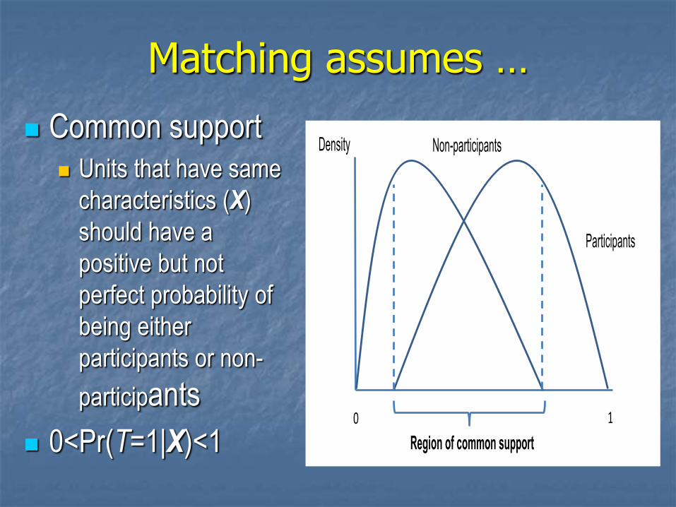
Matching assumes …

Common support Units that have same

characteristics (X)

should have a

positive but not

perfect probability of

being either

participants or non-

participants

0<Pr(T=1|X)<1

0 1

0

Density

Participants

Non-participants

Region of common support

Types of Matching

Covariate (or Direct) matching

Match a participant to a non-participant

using covariates

Propensity score matching

Match a participant to a non-participant

using propensity scores

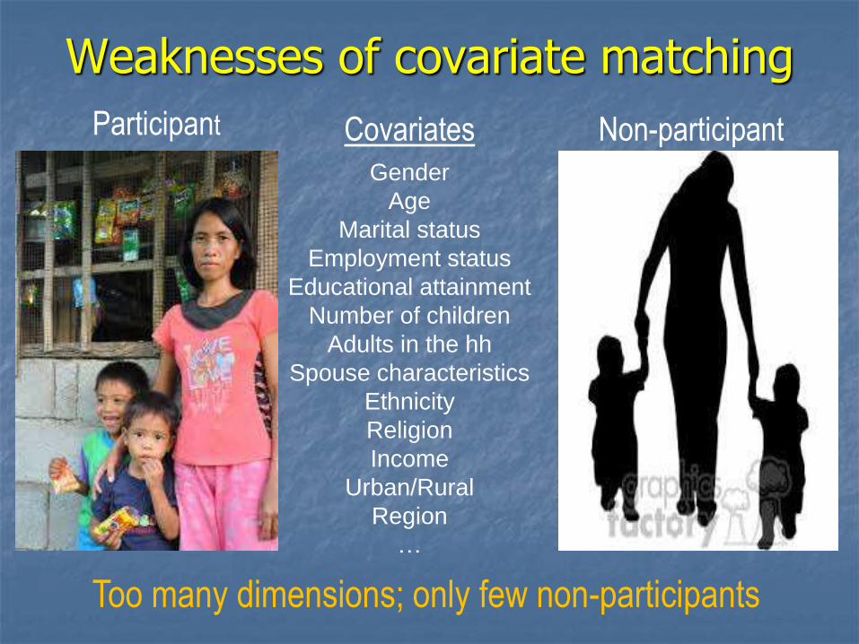
Weaknesses of covariate matching

Participant Non-participant

Gender

Age

Marital status

Employment status

Educational attainment

Number of children

Adults in the hh

Spouse characteristics

Ethnicity

Religion

Income

Urban/Rural

Region

…

Covariates

Too many dimensions; only few non-participants

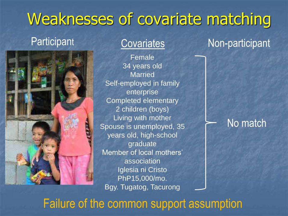
Weaknesses of covariate matching

Participant Non-participant Female

34 years old

Married

Self-employed in family

enterprise

Completed elementary

2 children (boys)

Living with mother

Spouse is unemployed, 35

years old, high-school

graduate

Member of local mothers’

association

Iglesia ni Cristo

PhP15,000/mo.

Bgy. Tugatog, Tacurong

Covariates

No match

Failure of the common support assumption

Dealing with the dimensionality problem

Match using propensity scores

The propensity score is the probability that an

individual will be in the treatment group given her

observed covariates (X).

Pr(T=1|X)=Pr(X) → “reduce the info in X into one

number (propensity score)”.

Intuition: Rather than match on each of the many

dimensions, match on a single dimension.

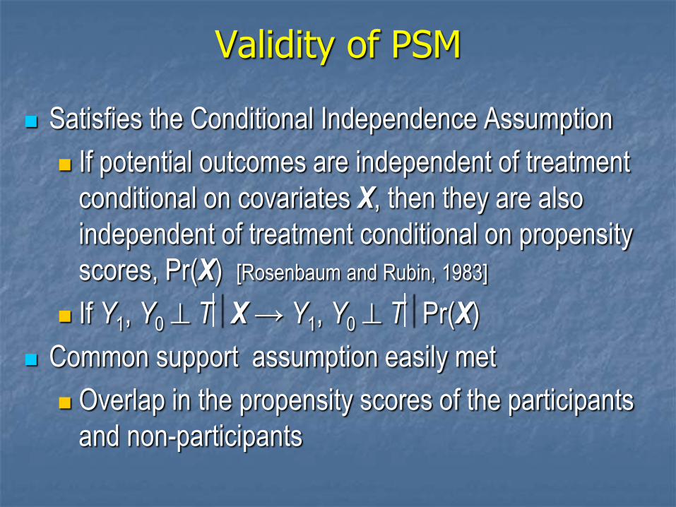
Validity of PSM

Satisfies the Conditional Independence Assumption

If potential outcomes are independent of treatment

conditional on covariates X, then they are also

independent of treatment conditional on propensity

scores, Pr(X) [Rosenbaum and Rubin, 1983]

If Y1, Y0 TX → Y1, Y0 TPr(X)

Common support assumption easily met

Overlap in the propensity scores of the participants

and non-participants

Step 1 in PSM

Choose the appropriate dataset

Ideally, the data on the participants and non-

participants should come from the same source (i.e.,

same survey, using same questionnaire) Poor in the poorest areas (participants) vs. poor in non-poor areas (non-

participants)

Same questions, but different time period

Have you received social health insurance benefits (before and after

universal health insurance coverage, or before and after a natural

disaster)

Different reference period or reference group

Incidence of child diarrhea in the last week vs. Incidence of diarrhea in

infants in the last 24 hours

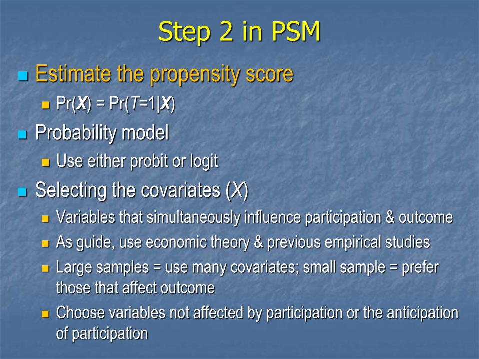
Step 2 in PSM

Estimate the propensity score Pr(X) = Pr(T=1|X)

Probability model

Use either probit or logit

Selecting the covariates (X)

Variables that simultaneously influence participation & outcome

As guide, use economic theory & previous empirical studies

Large samples = use many covariates; small sample = prefer

those that affect outcome

Choose variables not affected by participation or the anticipation

of participation

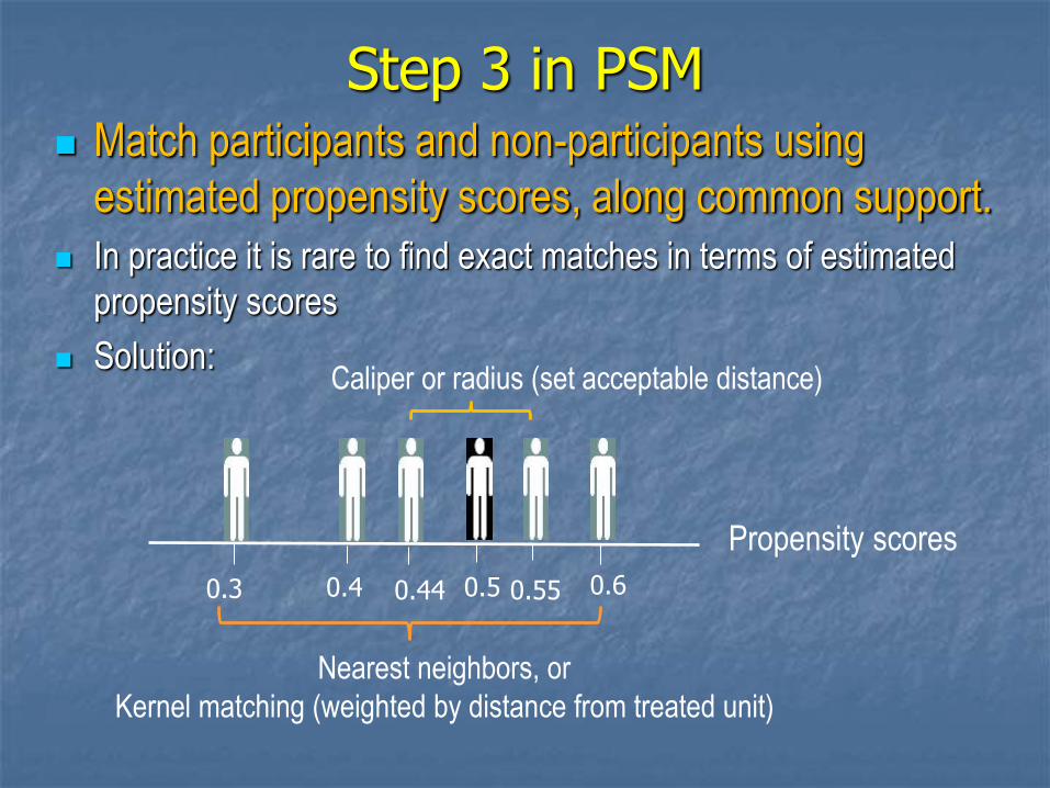
Step 3 in PSM Match participants and non-participants using

estimated propensity scores, along common support.

In practice it is rare to find exact matches in terms of estimated

propensity scores

Solution:

Propensity scores

0.55 0.5 0.4 0.6 0.3 0.44

Nearest neighbors, or

Kernel matching (weighted by distance from treated unit)

Caliper or radius (set acceptable distance)

Step 4 in PSM

Perform balancing tests: The participants and non-

participants should have balanced covariates.

Two-sample t-tests of means in the covariates: No significant

differences in the means

Comparison of standardized bias (difference in means ÷

standard deviation) before & after matching: Lower after

matching

Joint significance (F-tests): “zero” after matching

Psuedo-R2: lower after matching

Stratification test: no significant differences in the means of the

propensity scores of participants and non-participants included in

the stratum

Step 5 in PSM

Estimate the average treatment effects using

the participants and matched non-participants

Compute the effect of the treatment for each

match (i.e., difference in outcomes between

the participants and matched non-

participants)

Obtain the average of these conditional

treatment effects

Step 5 in PSM

Computing standard errors

Bootstrapping method = repeat estimation

several times from a randomly drawn sub-

sample of the whole samples and generate

standard errors of estimates (for kernel

matching)

Bias-adjusted robust standard errors (for

nearest neighbor)

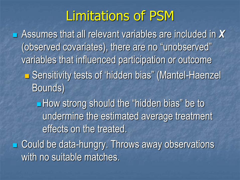
Limitations of PSM

Assumes that all relevant variables are included in X

(observed covariates), there are no “unobserved”

variables that influenced participation or outcome

Sensitivity tests of ‘hidden bias” (Mantel-Haenzel

Bounds)

How strong should the “hidden bias” be to

undermine the estimated average treatment

effects on the treated.

Could be data-hungry. Throws away observations

with no suitable matches.

Application: Estimating the impact of piped water and flush toilets on the incidence of child

diarrhea in rural Philippines

Dataset - NDHS

All rural households with children below 5 years old from

the 2008 round of the NDHS

Some of these children had diarrhea during the two-

week period prior to the interview

Treatment vs. control

Children in households with piped water vs.

children in households without piped water

Children in households with their own flush toilets

vs. children in households without their own flush

toilets.

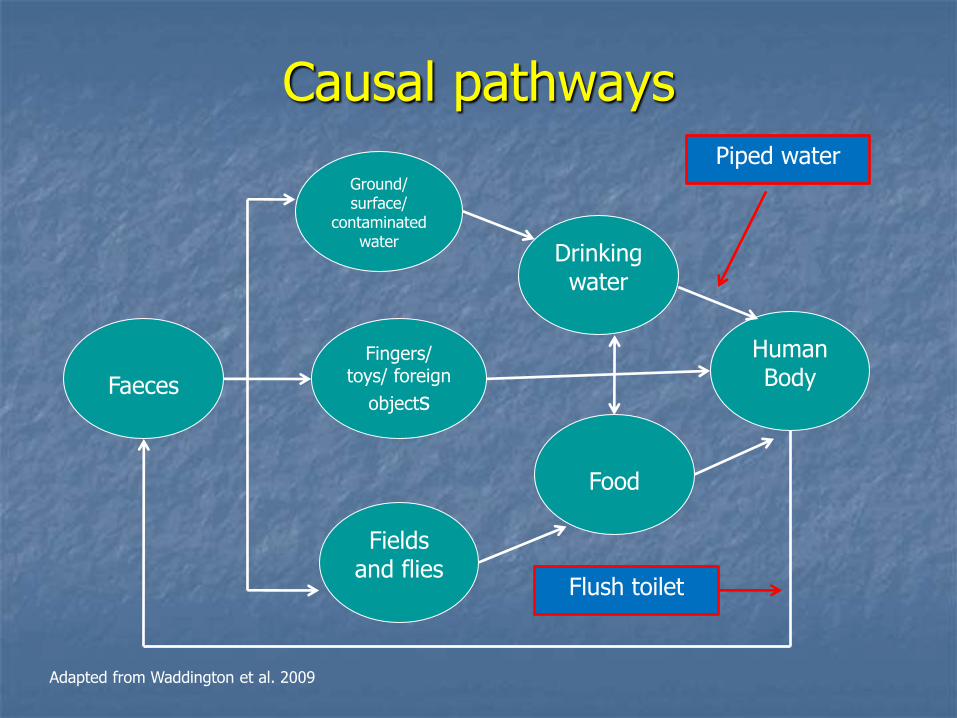
Causal pathways

Human Body

Drinking water

Food

Fingers/ toys/ foreign

objects

Ground/ surface/

contaminated water

Fields and flies

Faeces

Adapted from Waddington et al. 2009

Piped water

Flush toilet

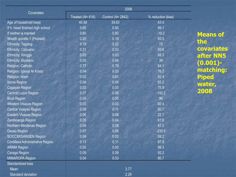
Covariates 2008

Treated (N= 616) Control (N= 2842) % reduction |bias|

Age of household head 40.58 39.83 43.4

If h. head finished high school 0.60 0.60 99.1

If mother is married 0.80 0.80 -19.2

Wealth quintile 1 (Poorest) 0.20 0.19 93.5

Ethnicity: Tagalog 0.19 0.22 73

Ethnicity: Cebuano 0.31 0.33 50.6

Ethnicity: Ilonggo 0.05 0.03 68.3

Ethnicity: Bicolano 0.05 0.04 39

Religion: Catholic 0.77 0.79 64.1

Religion: Iglesia Ni Kristo 0.04 0.03 76.7

Religion: Islam 0.02 0.01 92.4

Ilocos Region 0.04 0.04 83.2

Cagayan Region 0.03 0.03 75.9

Central Luzon Region 0.07 0.08 -142.2

Bicol Region 0.05 0.05 96

Western Visayas Region 0.03 0.03 92.4

Central Visayas Region 0.09 0.11 50.7

Eastern Visayas Region 0.06 0.08 22.1

Zamboanga Region 0.05 0.04 61.6

Northern Mindanao Region 0.09 0.08 81.2

Davao Region 0.07 0.06 -235.5

SOCCSKSARGEN Region 0.04 0.03 59.2

Cordillera Administrative Region 0.13 0.11 87.9

ARMM Region 0.00 0.00 99.3

Caraga Region 0.09 0.09 92.2

MIMAROPA Region 0.04 0.03 80.7

Standardized bias

Mean 3.77

Standard deviation 2.29

Pseudo R-squared (logit) 0.1726

Means of the covariates after NN5 (0.001)-matching: Piped water, 2008

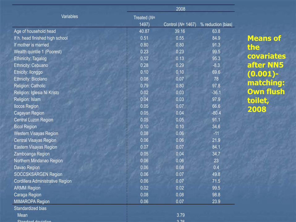
Means of the covariates after NN5 (0.001)-matching: Own flush toilet, 2008

Variables

2008

Treated (N=

1497) Control (N= 1467) % reduction |bias|

Age of household head 40.87 39.16 63.8

If h. head finished high school 0.51 0.55 84.9

If mother is married 0.80 0.80 91.3

Wealth quintile 1 (Poorest) 0.23 0.23 99.5

Ethinicity: Tagalog 0.12 0.13 95.3

Ethnicity: Cebuano 0.28 0.29 -8.3

Etnicity: Ilonggo 0.10 0.10 69.6

Ethnicity: Bicolano 0.08 0.07 78

Religion: Catholic 0.79 0.80 97.8

Religion: Iglesia Ni Kristo 0.02 0.03 -36.1

Religion: Islam 0.04 0.03 97.9

Ilocos Region 0.05 0.07 66.6

Cagayan Region 0.05 0.04 -80.4

Central Luzon Region 0.05 0.05 91.1

Bicol Region 0.10 0.10 34.6

Western Visayas Region 0.08 0.06 -11

Central Visayas Region 0.06 0.06 21.9

Eastern Visayas Region 0.07 0.07 84.1

Zamboanga Region 0.05 0.04 34.7

Northern Mindanao Region 0.06 0.06 23

Davao Region 0.06 0.08 0.4

SOCCSKSARGEN Region 0.06 0.07 49.8

Cordillera Administrative Region 0.06 0.07 71.5

ARMM Region 0.02 0.02 99.5

Caraga Region 0.08 0.08 98.8

MIMAROPA Region 0.06 0.07 23.9

Standardized bias

Mean 3.79

Standard deviation 3.76

Pseudo R-squared (logit) 0.2757

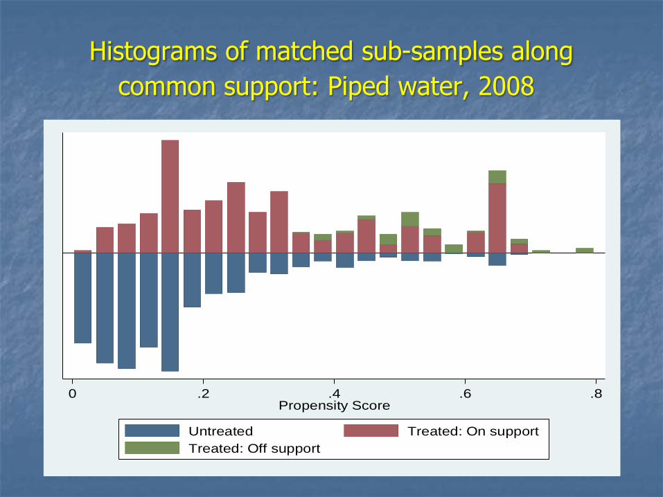
Histograms of matched sub-samples along

common support: Piped water, 2008

0 .2 .4 .6 .8Propensity Score

Untreated Treated: On support

Treated: Off support

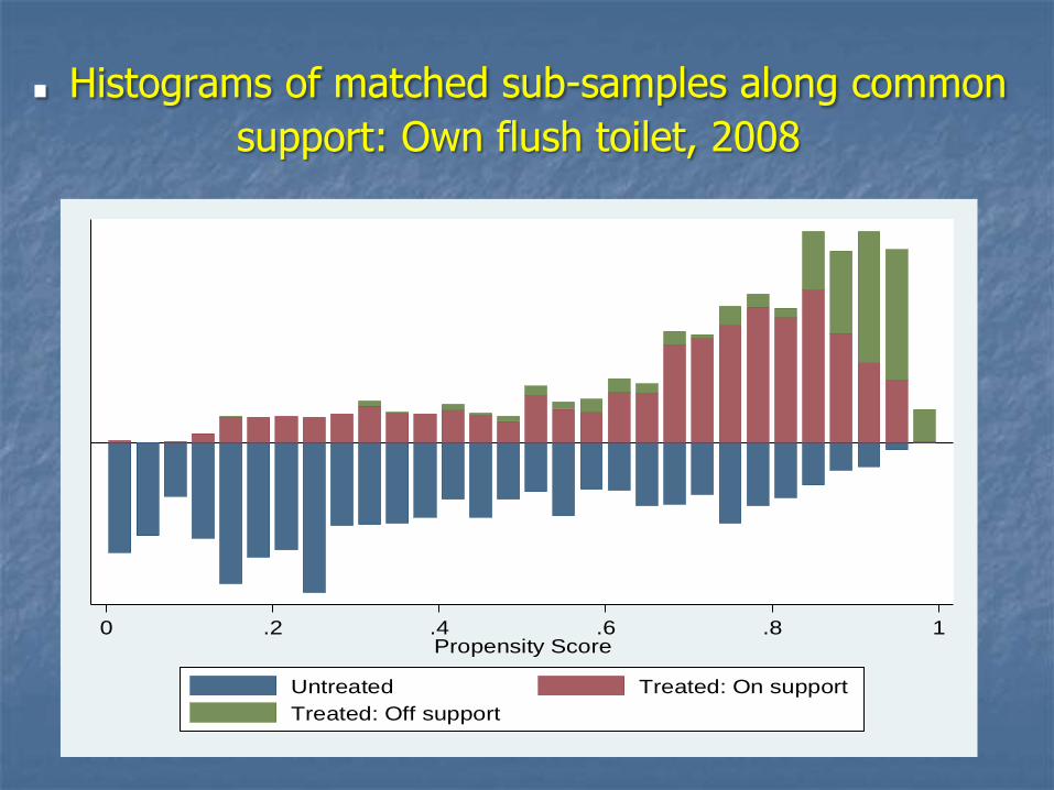
. Histograms of matched sub-samples along common

support: Own flush toilet, 2008

0 .2 .4 .6 .8 1Propensity Score

Untreated Treated: On support

Treated: Off support

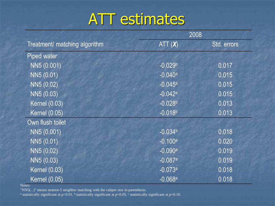
ATT estimates

Treatment/ matching algorithm

2008

ATT (X) Std. errors

Piped water

NN5 (0.001)

NN5 (0.01)

NN5 (0.02)

NN5 (0.03)

Kernel (0.03)

Kernel (0.05)

-0.029b

-0.040a

-0.045a

-0.042a

-0.028b

-0.018b

0.017

0.015

0.015

0.015

0.013

0.013

Own flush toilet

NN5 (0.001)

NN5 (0.01)

NN5 (0.02)

NN5 (0.03)

Kernel (0.03)

Kernel (0.05)

-0.034b

-0.100a

-0.090a

-0.087a

-0.073a

-0.068a

0.018

0.020

0.019

0.019

0.018

0.018 Notes: "NN5(...)" means nearest-5 neighbor matching with the caliper size in parenthesis. a statistically significant at p<0.01. b statistically significant at p<0.05. c statistically significant at p<0.10.

Sources and references J. Capuno, CA Tan, Jr. and VM Fabella (2013). Do piped water and flush

toilets prevent child diarrhea in rural Philippines? Asia Pacific Journal of Public

Health.

D. Evans (2010). Impact evaluation methods: Difference in difference &

matching. Africa Program for education impact evaluation and World Bank.

P. Gertler et al. (2011). Impact evaluation in practice. Washington, DC: The

World Bank.

S. Khandker et al. (2010). Handbook on impact evaluation. Washington, DC:

The World Bank.

A. Orbeta, Jr. and R. B. Mallari (2013). Impact evaluation training for DSWD

Staff. DSWD.

H. White (2009). Theory-based impact evaluation: principles and practice. 3ie

working paper 3. 3ie, New Delhi.

H. White (2012). Quality impact evaluation: An introductory workshop. 3ie, New

Delhi.

Thank you!