1

 

Credibility of propensity score matching estimates. An example from Fair Trade certification of coffee producers

Nicolas Lampach and Ulrich B. Morawetz

This article has been published in “Applied Economics”. Please download the edited version from:

http://dx.doi.org/10.1080/00036846.2016.1153795

and use the information provided there for citation. Thank you.

Abstract

Propensity score matching (PSM) is an increasingly popular method for evaluation studies in

agricultural and development economics. However, statisticians and econometricians have stressed

that results rely on untestable assumptions, and therefore guidelines for researchers on how to improve

credibility have been developed. We follow one of these guidelines with a data set analyzed by other

authors to evaluate the impact of Fair Trade certification on the income of coffee producers. We

provide thereby a best practice example of how to evaluate the credibility of PSM estimates. We find

that a thorough assessment of the assumptions made renders the data we use not suitable for a credible

PSM estimation of the effects of treatment. We conclude that the debate about the impact of Fair

Trade certification would greatly benefit from a detailed reporting of credibility checking.

JEL classification: Q13; Q12; C19

Keywords: Credibility; Propensity Score Matching; Evaluation; Coffee Certification; Ethiopia

Running title: Credibility of PSM: Fair Trade certification of coffee producers

Corresponding author: Ulrich B. Morawetz: University of Natural Resources and Life Sciences, Vienna (BOKU), Feistmantelstr. 4, 1180 Vienna, Austria, +43/1/47654-3672, Email: ulrich.morawetz@boku.ac.at

Nicolas Lampach: BETA, CNRS and University of Strasbourg, Avenue de la Forêt Noire 61, 67085 Strasbourg, France, +33/0/368852091, Email: nlampach@unistra.fr

Acknowledgements:

Grateful thanks to Jasjeet S. Sekhon from the University of California (UC Berkely), Bruno Rodrigues and Sandrine Spaeter from the University of Strasbourg (BETA, CNRS) and Klaus Salhofer from University of Natural Resources and Life Sciences Vienna (BOKU) for giving us helpful advice, thanks to Pradyot R. Jena from the International Maize and Wheat Improvement Center (CIMMYT) for providing us with accurate data, to Liz Lucas for editing and for the useful comments from participants during the poster presentation at the Augustin Cournot Doctoral Days event which took place in Strasbourg on April 11-12, 2014. Thanks for suggestions for improvements to the anonymous reviewers. All errors are ours.

2

 

1. Introduction

Propensity score matching (PSM) is a method which allows the use of observational data to estimate

the effect of a treatment. It is based on a very appealing idea: the pairwise comparison between the

treated and the not treated is limited to observations which are, except for the treatment, identical.

PSM has become a frequently-used method for evaluation studies published in agricultural economics

journals. For example, it has been used to assess the effect of agricultural policy on environmental

outcomes (Chabé-Ferret and Subervie 2013; Pufahl and Weiss 2009), to estimate the effect of

agricultural policy on land values (Michalek, Ciaian, and Kancs 2014) and to estimate the effect of

using metal silos to prevent storage losses of Kenyan farmers (Gitonga et al. 2013). It has also been

used to evaluate the impact of Fair Trade certification on the livelihoods of coffee producers

(Chiputwa, Spielman, and Qaim 2015; Jena et al. 2012; Ruben and Fort 2012).

However, statisticians and econometricians warn that, while propensity score matching is a potentially

useful econometric tool, it does not represent a general solution to the evaluation problem (Smith and

Todd 2005). Several studies have shown that even with very thorough application of the method it is

not always possible to replicate results retrieved from randomized controlled trails (Smith and Todd

2005; Peikes, Moreno, and Orzol 2008; Wilde and Hollister 2007). Blundell et al. (2005) remind

readers that, as in regression-based approaches, the central issue in the matching method is choosing

the appropriate covariates to fulfill the unconfoundedness assumption. As with all other econometric

methods, unconfoundedness cannot be tested directly (Imbens 2015).

To help increase the credibility of results from PSM, several authors have written best practice

guidelines on how to apply PSM (Caliendo and Kopeinig 2008; Imbens 2015). They provide step-by-

step descriptions of how to conduct PSM. The guidance from Caliendo and Kopeinig (2008) is

organized in five steps: 1. propensity score estimation; 2. choosing a matching algorithm; 3. checking

common support; 4. matching quality assessment and estimation of effects; 5. sensitivity analysis. In

order to be applicable for multiple cases, the guidelines are kept rather general. The purpose of this

article is to use the guidelines proposed by Caliendo and Kopeinig (2008) and apply them to an

example from the field of agricultural economics, thereby giving a best practice example which will

help to pinpoint problems faced when applying the PSM method.

3

 

As an example we opt for the debate about the impact of coffee certification on the livelihood of

producers. At its core the debate is about whether Fair Trade1 certification makes economic sense, and

whether it actually improves the livelihoods of coffee producers (Dragusanu, Giovannucci, and Nunn

2014). Dammert and Mohan (2014) demonstrate that many of the recent evaluations of Fair Trade face

severe methodological challenges. Three recent papers have used PSM to estimate the effect of Fair

Trade certification (Chiputwa, Spielman, and Qaim 2015; Jena et al. 2012; Ruben and Fort 2012). We

use the data provided in one of these articles to demonstrate how the five steps in the guidelines of

Caliendo and Kopeinig (2008) may be applied to increase credibility of PSM estimates. While we do

not provide new data, we contribute to a better understanding of how reliable results from matching

analysis about the impacts of coffee certification schemes might look. We also provide the code for

open-source software to make it easy for readers to apply the steps by themselves.

The remainder of this paper is organized as follows: section 2 presents the two fundamental

assumptions of PSM; in section 3 we provide a the best practice example of how to apply a guideline

for evaluation by PSM of Fair Trade certification; section 4 concludes the paper by summarizing the

lessons learned when applying the guidelines, and by recommending points which are vital for

credible results in future research on Fair Trade certification.

2. Assumptions required for unbiased PSM estimates

To ensure that the data analysis leads to an unbiased estimate of the treatment effect, both the

unconfoundedness2 as well as the common support3 assumptions need to be fulfilled (Caliendo and

Kopeinig 2008). Unconfoundedness implies that the systematic differences in outcomes between

treated and untreated control observations with the same observable characteristics are entirely

attributable to the treatment. The unconfoundedness assumption is untestable due to the impossibility

of testing whether there is an omitted variable influencing the outcome and the treatment alike.

Researchers have to rely on theory and, if applicable, on non-linear instrument variable regression to

specify their balancing scores model. Hence all variables that influence the treatment assignment and

the outcomes simultaneously have to be modelled (Caliendo and Kopeinig 2008).

The unconfoundedness assumption is clearly more difficult to fulfil if no pre-treatment observations

are available: the covariates used for matching must not be modified by the treatment (Caliendo and

                                                            1 In 2012 the US Fair Trade organization split from the umbrella organization (Dragusanu, Giovannucci, and Nunn 2014). When we write “Fair Trade” we refer to the general initiative and movement. 2 Also called ‘ignorability’ 3 In the literature also referred to as ‘overlap’ 

4

 

Kopeinig 2008). If pre-treatment observations are available, lagged outcomes can also be used as

‘pseudo outcome’ for a plausibility test of the unconfoundedness assumption (Imbens 2015). If the

estimated treatment effect differs from zero, the unconfoundedness assumption is less plausible.

The common support assumption requires every observed covariate combination to be in the treatment

and in the control group. As a consequence, researchers frequently drop observations which do not

have suitable counterparts or, more precisely, which are not fitting for comparison. If one is interested

only in the average treatment effect on the treated (ATT) a weaker assumption is sufficient: for the

treated observations only, suitable control counterparts are necessary (in this case, only treated

observations are dropped). Clearly, dropping observations modifies the quantity being estimated.

3. Example: the treatment effect of Fair Trade certification of coffee

Fair Trade is an alternative approach to conventional trade based on a partnership agreement between

producers and traders, businesses and consumers. As consumers usually pay a price premium for Fair

Trade products, evaluation of the impact of Fair Trade on producers’ livelihoods is crucial for the

justification of the premium.

Dragusanu et al. (2014) summarize in their survey that empirical evidence, based primarily on

conditional correlations, suggests that Fair Trade does achieve many of its intended goals (higher

average prices for farmers, greater access to credit, more stable perceived economic environment and

more probable environmentally-friendly practices), although these effects are on a comparatively

modest scale. In another recent survey Dammert and Mohan (2014) explain that the only-modest effect

of Fair Trade on profits is driven by the limited world market demand for Fair Trade coffee.

Consequently, only a fraction of producers’ output can realize Fair Trade premiums (Dammert and

Mohan 2014). The survey by Dammert and Mohan (2014) also shows that many publications about

the effect of Fair Trade certification have severe methodological shortcomings.

Three recent articles which have used PSM to analyze the impact of Fair Trade certification have been

published in established scientific journals. Chiputwa et al. (2015) find that Fair Trade certification in

Uganda increases household living standards and reduces the prevalence and depth of poverty.

Organic and UTZ certification, on the other hand, do not have a significant influence on these

indicators. Ruben and Fort (2012) find modest positive direct effects of coffee certification in Peru on

income and production, but also significant changes in organization, use of inputs, wealth, assets and

attitude to risk. Jena et al. (2012) do not find a significant influence of Fair Trade on per capita

income, total income, and yield per ha, but find a small, statistically significant influence on per capita

consumption.

5

 

Table 1 summarizes how these three journal articles differ in the number of observations, data

structure, covariates and modeling variations they present to the reader. Only one of the studies uses

before-treatment observations, none presents alternative choices of covariates, and only one shares the

results of a sensitivity analysis with the reader. The article by Jena et al. (2012) is the only one where

data and computer code are available from the journal’s webpage. We use this article to demonstrate

the five steps of Caliendo and Kopeinig (2008).

[Table1 here]

Jena et al. (2012) define Fair Trade certified farms as those being a member of a Fair Trade

cooperative. They collected data from 249 coffee-producing farmers from four Fair Trade certified

cooperatives and two non-certified cooperatives. By using a propensity score matching estimator with

cross-section data they find a small — but significant — treatment effect of certification on per capita

consumption of 0.79 Ethiopian Birr (the 1.25 USD poverty line translates to 5.47 Ethiopian Birr per

capita income per day). On the other hand, they find no significant effect of certification on per capita

income, log total income, or yield per ha.

They suggest two reasons for the economically-insignificant effects of certification: firstly, the prices

paid by the certified cooperatives are not different from the prices paid by the non-certified

cooperatives, and secondly, both certified and non-certified famers sell a substantial part of their

coffee harvest (75%) to private traders who, incidentally, pay a relatively higher price to non-certified

farmers. From qualitative interviews they conclude that the institutional arrangements of the

cooperatives are heterogeneous, and that the effect of certification hinges mainly on the institutional

strength of cooperatives. They explain that the insignificant effect of certification on the income levels

of the farmers indicates that there is a failure of farmers’ organizations rather than a failure of

certification itself.

3.1. Empirical Approach

For the demonstration of how to make PSM more credible we follow the five steps described by

Caliendo and Kopeinig (2008). For the sake of brevity, we restrict our replication to the outcome

variables per capita income, log total income and per capita consumption and refrain from using yield

per ha which is the fourth outcome used by Jena et al. (2012) but has less observations due to missing

data.

6

 

The first step in Caliendo and Kopeinig (2008) is the propensity score estimation. For the binary case

this primarily involves the choice of the variables used as covariates and their functional form. The

data at hand pose several difficulties for a proper modeling. Firstly, to fulfil the unconfoundedness

assumption covariates should influence the probability of being certified and the outcome alike, but

covariates should not be influenced by certification. This is difficult in the case of cross-section data as

no pre-certification covariates are available. Secondly, it is not known for how long the farmers have

been members of the cooperative. Since it can be expected that some of the effects of certification will

take a while to materialize it is impossible to know if the outcomes from certification are already

observable. Thirdly, it is not known what proportion of the crops is sold to the cooperative and

therefore which price regime applied. Given these shortcomings in the data, we use the data at hand to

fit the model as well as possible.

For the approach to choosing the covariates, we refer to Caliendo and Kopeinig (2008) who

summarize the literature thus: ‘the economic theory, a sound knowledge of previous research and also

information about the institutional settings should guide the researcher in building up the model’. The

logical starting point is the literature closest to the problem at hand. Consequently we start with the

logit model used by Jena et al. (2012) to reproduce exactly their results (first column in Table 2).

Additionally we suggest an ‘alternative model’ by choosing different covariates (fourth, fifth and sixth

columns). We review other articles on the impact of coffee certification and elicit which covariates

might be added to the alternative model. We then consider economic theory and institutional settings

and check the MatchBalances of the covariates. A MatchBalance is a summary of descriptive statistics

and tests to check if the treated (certified) and control (non-certified) observations have the same

distribution in observed variables. For checking the MatchBalance we follow the advice of Walter and

Sekhon (2011) to include higher-order terms of the variables. For the choice of covariates, though, we

add high-order terms only if linear terms are unbalanced according to the MatchBalance, as

recommended by Caliendo and Kopeinig (2008). An additional decision researcher’s face is whether

to use propensity scores lying in the range between the values 0 and 1, or linear predictions of the logit

model. Diamond and Sekhon (2013) argue that linear predictions should be used as they are often

closer to being normally distributed. We use propensity scores for the original set of variables and

linear predictions for the alternative model.

[Table 2 here]

7

 

The second step in Caliendo and Kopeinig (2008) is choosing a matching algorithm. Jena et al. (2012)

use Nearest Neighbor Matching (NN) which we reproduce exactly as a reference (Rubin 1973). In

addition we apply two alternative matching methods to check the influence of the choice of the

matching algorithm. The first matching method is Mahalanobis-distance Matching (MM) which

differs from Nearest Neighbor Matching by not relying on estimated propensity scores but directly

minimizes the Mahalanobis-distance between the covariates (Rosenbaum and Rubin 1985). The third

matching method we consider is Genetic Matching (GM), which minimizes a generalized

Mahalanobis-distance but uses an optimization routine to find an optimal weight for each covariate

(Diamond and Sekhon 2013). Genetic Matching improves covariate balance over the usual matching

methods, especially when the variables are not ellipsoidally distributed (e.g. normal- or t-distributed).

An extensive Monte Carlo study for the choice of the matching algorithm, as demonstrated in Huber et

al.(2013), will in most cases not be feasible. First, the data set must be very large to treat the sample as

coming from an infinite population and, second, the simulation itself is computational demanding and

time-consuming.. We intended to choose matching methods with appropriate theoretical properties

which demonstrate the influence of the choice of the matching method on our results.

Researchers face several other decisions when applying each of these matching methods. One is

whether matching should be done with replacement. As the sample analyzed here includes more

treated than control observations, matching without replacement would imply further reducing the

small sample. Similarly, the caliper-distance of a recommended width of 0.2 standard errors (Austin

2011) drastically reduces the resulting number of matches4. Finally, the distance-tolerance was set to a

precision equal to 1E-06, which allows us to replicate exactly the original results. Ties are dealt with

by calculating weighted averages to avoid randomness in the results through random breaking of ties.

The third step in Caliendo and Kopeinig (2008) implies checking the common support of treated and

control observations. We apply two different selection rules for observations and additionally compare

them through visual analysis. Firstly, for the reproduction of the original results, we apply the minima-

maxima rule for the average treatment effect (ATE): we use only those control group observations

where the propensity score is higher than the lowest propensity score of the treatment group, and only

those treatment group observations where the propensity score is lower than the highest propensity

score of the control group5.

As a second method, we apply the CHIM (Crump, Hotz, Imbens and Mitnik) approach developed by

(Crump et al. 2009) through the theory of asymptotic efficiency bounds. The main advantage of this

approach is that it reduces the variance of the estimated treatment effects and improves robustness                                                             4 when applying caliper-distances, we found less than 10 matched observations. 5 Interestingly, JENA ET AL. (2012) do not use the weaker rule for ATT which would result in not dropping control observations, even though they estimate the ATT. 

8

 

through trimming observations which have a high leverage (Imbens 2015). We apply the CHIM

approach for the alternative model.

The fourth step involves the assessment of the matching quality and the estimation of the treatment

effects. The main idea is to appraise the accuracy of the matching procedure in order to balance the

distribution of relevant variables in both control and treatment groups. To assess the MatchBalance we

use standardized differences (Std. Diff.) recommended by Rosenbaum and Rubin (1985) which should

not exceed the value of 20. Similarly, the ratio of variance should be approximate to the value of 1

(Rubin 2001). We also report p-values on the difference of the mean of treated and observed

observations. In ex-post impact evaluation the ATT is usually considered more relevant than the ATE.

We do not see a need to estimate alternative measures for the treatment effect as we consider it the

best choice in this context. For the estimation of the variance of the ATT, we use the Abadie-Imbens

standard error (Abadie and Imbens 2006) which corrects for uncertainty in Mahalanobis-distance

Matching and Genetic Matching.

The fifth step entails the sensitivity analysis. To test the results for their sensitivity to the

unconfoundedness assumption we apply Wilcoxon's Sign-Rank and Hodges-Lehmann tests

(Rosenbaum 2002, 114 and 116). The tests reveal whether the estimated treatment effects are still

significant in the case that the matched pairs did not have equal propensity scores because of a

violation of the unconfoundedness assumption. The magnitude of the violation is measured by the

factor by which the odds of being certified differ.

We analyze the data with the open-source software R (R Development Core Team 2015) and the R-

packages ‘Matching’ v4.8-3.4 (Sekhon 2011), ‘rgenoud’ v5.7-12 (Walter and Sekhon 2011) and

‘rbounds’ v2.0 (Keele 2010). Interested readers are welcome to download our code and data together

with a detailed appendix from the webpage of the journal.

3.2. Results

As certification is based on cooperative membership, data on the cooperative level are first discussed,

and then data on certified and non-certified producers. On the level of cooperatives, the means of

observable variables are mostly not statistically different: only for ‘Access to non-farm income’ and

‘Size of Farm’ the ANOVA based F-test is significant on a 5% level, refuting the hypothesis of

equality in the mean value comparing cooperatives (see Tables A1a, A1b, A1c in the online appendix

for details). Comparing observable variables of Fair Trade certified with non-certified producers the

picture is more diverse: all variables describing the household head or the household itself are

9

 

significantly different, except for education where the hypothesis of equal means cannot be rejected

(for details see Table A1a in the online appendix). With respect to farm characteristics, there is no

statistically-significant difference between certified and non-certified farms with respect to most of the

variables (size of farm, price of coffee paid by the cooperatives, value of livestock, damage by floods

or droughts, income from coffee, total household income and coffee yield). We find a difference

between certified and conventional farms with respect to price for dried coffee paid by traders (15%

lower for members of certified cooperatives), area of land under coffee (30 % more land under coffee

by members of certified cooperatives), per capita income (47% lower for members of certified

cooperatives), and per capita consumption (27% higher for members of certified cooperatives). See

Table A1b in the online appendix for details.

The logit model for estimating propensity scores used by Jena et al. (2012) explains the probability of

a farm being certified by the characteristics of the household head: (age, age squared, education and

gender); household characteristics: (access to non-farming income, dependency ratio6, experience in

coffee production and access to credit); and by farm characteristics: (land area, recent exposure to

flood and drought shocks). Table 1 summarizes the covariates used by other authors applying PSM to

estimate the impact of coffee certification. Characteristics of the household head similar to those used

by Jena et al. (2012) are included in all studies. However, household and farm characteristics used as

covariates are quite heterogeneous. This is likely the consequence of household and farm

characteristics being seen as exogeneous, but farm characteristics are potentially endogeneous

(compare Dragusanu et al. (2014). Based on the literature and on the variables available in the data set,

we added land coffee area, household size and livestock as additional covariates. Checking

institutional settings, it transpired that Fair Trade policies offer pre-finance to producers (Fairtrade

International 2015), which renders the variable access to credit incompatible with the

unconfoundedness assumption in the event of cross-section data (even if these Fair Trade policies

should not apply it is likely that credit worthiness is influenced by certification). Using economic

theory, one could object that land area, livestock, land coffee area and household size might be

influenced by certification and therefore would not be suitable in the model: if there are costs

associated with certification, households might buy or sell livestock to cover them, or if there are

production requirements for certification, land area in coffee is also likely to be affected.7 Adding

these variables might introduce bias just as much as omitting them. Additional information (in

particular pre-treatment information) is necessary to derive unbiased treatment effects or at least to run

indirect tests of exogeneity. For the sake of demonstrating the next four steps of Caliendo and

Kopeinig (2008) we include these four variables: dropping them leads to the same main conclusions as

including them.

                                                            6 Household members below 14 and above 65 years divided by the rest of the household members. 7 We thank one of the anonymous reviewers for making this explicit. 

10

 

The MatchBalances after matching were particularly unbalanced for the covariates recent exposure to

flood and drought shocks and access to non-farming income. Both covariates might influence coffee

production but not necessarily the likelihood of certification. Since including unbalanced covariates

can induce bias, we opted to drop these two covariates. Hence the covariates of the final alternative

model contain the following variables: age of the head of household; dependency ratio; household

size; land area; land coffee area; livestock; education; gender; and experience in coffee production.

The estimated coefficients for the two logit model specifications are available in the online appendix

as Table A2.

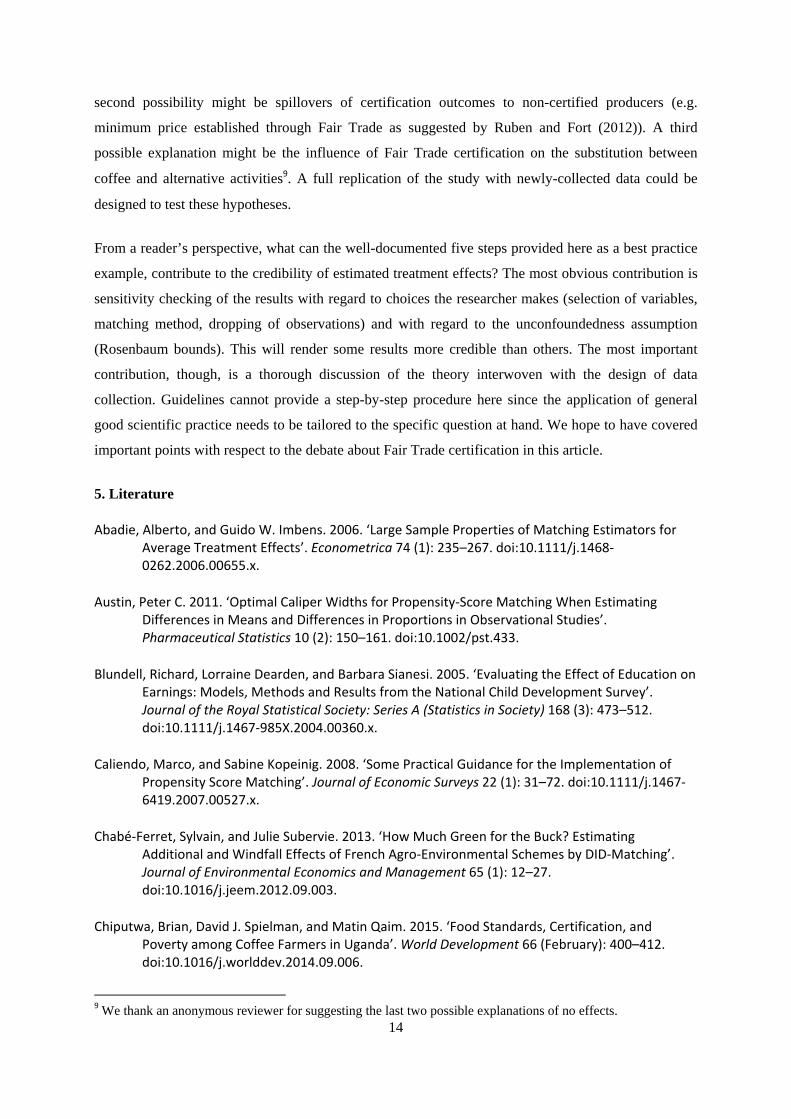
A histogram of the estimated propensity scores based on the original covariates shows that there are

three treated observations with propensity scores below 0.2, and 9 control observations with

propensity scores above 0.8. For the propensity scores based on the covariates of the alternative

model, there are 7 treated observations with propensity scores below 0.2, and 2 control observations

with propensity scores above 0.8 (see the online appendix Figure A1).

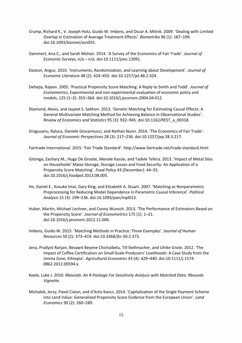
Applying the minima-maxima rule to the estimated propensity scores from the logit model with the

original covariates results in dropping 33 of the 164 treated observations and one of the 82 control

observations. The model with the original covariates has therefore 212 observations of which 131 are

certified. Applying the CHIM approach to the estimated propensity scores with the alternative

covariates results in dropping 32 of the 152 treatment observations and two of the 81 control

observations which are above the cutoff point of 0.899 (none of the observations were below the lower

cutoff point of 0.101)8. The model with the alternative covariates has therefore 199 observations of

which 120 are certified. See also online appendix Figure A1 and A2.

The matching quality assessment, as part of step four in Caliendo and Kopeinig (2008), is based on the

MatchBalances (see the online appendix Tables A3 to A8). The model with the original set of

variables results in low p-values for the t-tests for all variables, a standardized difference higher than

20 for almost all covariates, and a ratio of variance departing strongly from 1 for the covariates access

to non-farming income, land area squared, recent exposure to flood and drought shocks, gender, and

access to credit. The MatchBalances from Mahalanobis-distance Matching and Genetic Matching

have more favourable values for many, but not for all covariates. Turning to the MatchBalances of the

alternative model, Nearest Neighbor and Mahalanobis-distance Matching again have unbalanced

covariates according to at least one of the three criteria. For the MatchBalance from Genetic Matching

only the covariates dependency ratio squared, land area squared and livestock (squared and linear) are                                                             8 The number of observations differs between models with different covariates because of missing values in some of the covariates.

11

 

clearly unbalanced. As the choice of the variables was done checking the MatchBalance of Genetic

Matching, it is not surprising that Genetic Matching performs relatively well.

Graphically, the kernel density distributions of the propensity scores after matching for the six models

show a reasonable overlap of treated and control observations (see Figure A3 in the appendix).

Comparing the three matching approaches, the predictions for the estimated propensity scores higher

than 0.7 are covered better by Nearest Neighbor Matching than by Mahalanobis-distance and Genetic

Matching.

Turning to the estimated average treatment effect on the treated (see Table 3), no model specification

found a statistically significant effect of certification on per capita income or log total income of the

households. For the outcome per capita consumption, only the original model by Jena et al. (2012)

showed a significant impact of certification. The per capita consumption per day is estimated to be

0.79 Birr, with the average per capita consumption per day in the sample being 1.75 Birr. The five

other model specifications failed to find a significant influence of certification on per capita

consumption. Due to missing covariates the alternative set of explanatory models led to 13

observations being dropped.

[Table 3 here]

The last step is the sensitivity analysis. The Wilcoxon Ranks-Sign test shows that the effect of

certification on per capita consumption would vanish if an unobserved covariate increased the odds of

certification by more than a factor of 1.5. The lower and the upper bounds of the Hodges-Lehmann

estimates capture the range in which the treatment effect changes in the case of an unobserved

covariate bias. According to the Hodges-Lehmann point estimates, the difference between the treated

and the control observations for the original model with Nearest Neighbor matching is equal to 0.45

Birr per capita consumption per day, although this difference extends to a range of between 0.26 and

0.66 Birr per capita consumption per day if the odds of certification of equal observations are mis-

estimated by a factor of 1.25. For a factor of 2 (certified farmers with equal covariates as non-certified

farmers are twice as likely to be certified), this range extends from -0.04 to 1.16 Birr per capita

consumption per day.

4. Conclusions

12

 

In our case study of Fair Trade coffee certification we find that the data do not support the hypothesis

that there is, on average, an effect of membership of a Fair Trade certified cooperative on per capita

income, log total income and per capita consumption. Several clarifications need to be made to

understand this result.

Firstly, the proportion of crops sold under Fair Trade conditions at the producer level is not known.

This blurs the definition of what the treatment ‘certification’ actually means. The design of the survey

is not suitable for estimating the effect of certification, but instead we estimate the effect of

cooperative membership. The percentage of output actually going to Fair Trade markets is an issue in

many Fair Trade organizations, and consequently it would be necessary to consider it explicitly in

evaluation studies (Dammert and Mohan 2014).

Secondly, the design of the survey does not provide pre-treatment observations. Consequently, the

covariates used might be influenced by the certification (e.g. access to credit or land under coffee)

which will cause biases in an unknown direction, even if covariates are balanced. If the compared

producers have joined the cooperative at different times, it would be important to match pairs which

are similar prior to joining the cooperative (Rosenbaum 2010, 223). This is not possible with the data

at hand. The direction of the resulting bias is not known. The unconfoundedness assumption is not

fulfilled, therefore we do not know what causes our result of ‘no effect’. As our small survey of PSM

studies about certification has shown, it is not uncommon for pre-treatment observations to be missing,

even in well-established journals.

Thirdly, the propensity score overlap of treatment observations by control observations is reasonable

in relative terms, but rather poor in absolute terms (56 certified observations with a propensity score

higher than 0.8 but only 9 control observations in the case of the original specification). The rather low

number in absolute terms makes the results susceptible to the modeling choices (e.g. through missing

values in some of the covariates or through the choice of the matching algorithm). The common

support assumption is questionable. No general conclusions about different matching approaches are

possible due to the low absolute number of observations.

With the unconfoundedness and the common overlap assumption being questionable, the main result

of ‘no significant effect’ is hard to justify. Our only result is that the data do not support any

conclusion of the effect of membership in a certified cooperation. This is a major point in the

interpretation of the results and it is important to be explicit on this point. Obviously, being explicit on

this difference is only possible if proper assumption checking has been reported. Finally, the influence

of dropped variables (34 due to the common support restriction and 13 due to missing variables in the

alternative set of covariates from 246) is unknown and would require a separate discussion.

13

 

If we disregard the uncertainties about the unconfoundedness assumption, the estimated treatment

effects suggest that there is no significant difference in income between producers from certified and

producers from non-certified cooperatives. However, this result needs to be interpreted as certification

making a difference: the price for non-certified producers is, on average, 15% higher than for certified

producers. With 75% of the crop sold to private traders (Jena et al. 2012), the difference in revenue is

not negligible. Thus producers from certified cooperatives must have lower costs, higher yields, better

storage facilities or other sources of income. Unfortunately the data do not support an investigation

into what the actual reason might be. Also it is unfortunately not known why traders pay members of

certified cooperatives less.

This article shows how the application of readily available tools can make a difference in the

conclusions drawn from estimated PSM effects. This is captured on two levels. Firstly, the estimated

treatment effects are not credible because the unconfoundedness assumption is not met. The

conclusion is not ‘no effect’ but ‘no result’. Secondly, even if one is ready to accept that the

underlying assumptions are fulfilled, it is critical to apply a sensitivity analysis. Indeed, reporting a

significant effect without a sensitivity analysis has already lead to a questionable citation with the

results discussed; Chiputwa et al. (2015) cite Jena et al. (2012): ‘They showed that certification

contributes to higher incomes among coffee farmers, but the impact on poverty was insignificant.’

We saw that at least for the case of Fair Trade coffee certification, even in well-established journals

the number of possible alternative model specifications reported is quite limited. The importance of

the choice of covariates has already been stressed by others (Dehejia 2005; Ho et al. 2007). Ho et al.

(2007) have suggested a method of preprocessing the data and making the selection of the covariates

less opaque. If one sticks to PSM, though, it needs to be kept in mind that the unconfoundedness

assumption is central in PSM but cannot be tested. The techniques shown in this article are minimum

requirements, which each PSM study should report in order to make the paper credible. With online

appendices usually not restricting the length of papers, we wonder why these sensitivity checks are not

requested by reviewers.

We did not go into the issue of proper survey design. Rosenbaum (2010, 6) reminds readers that the

most plausible alternative explanations for an actual treatment effect need to be tested as well (and

considered in the survey design). These alternatives have to be described before a survey starts,

documented in a study protocol, and the data collected need to allow testing these alternatives. A

similar view is put forward by Deaton (2010), who stresses the importance of theory to make progress

in empirical research. In our case study, for example, a thorough theoretical discussion might lead to

alternative explanations for (no) treatment effect. One possible explanation might be the heterogeneity

of institutional strengths of the cooperatives, as qualitative research by Jena et al. (2012) suggests. A

14

 

second possibility might be spillovers of certification outcomes to non-certified producers (e.g.

minimum price established through Fair Trade as suggested by Ruben and Fort (2012)). A third

possible explanation might be the influence of Fair Trade certification on the substitution between

coffee and alternative activities9. A full replication of the study with newly-collected data could be

designed to test these hypotheses.

From a reader’s perspective, what can the well-documented five steps provided here as a best practice

example, contribute to the credibility of estimated treatment effects? The most obvious contribution is

sensitivity checking of the results with regard to choices the researcher makes (selection of variables,

matching method, dropping of observations) and with regard to the unconfoundedness assumption

(Rosenbaum bounds). This will render some results more credible than others. The most important

contribution, though, is a thorough discussion of the theory interwoven with the design of data

collection. Guidelines cannot provide a step-by-step procedure here since the application of general

good scientific practice needs to be tailored to the specific question at hand. We hope to have covered

important points with respect to the debate about Fair Trade certification in this article.

5. Literature

Abadie, Alberto, and Guido W. Imbens. 2006. ‘Large Sample Properties of Matching Estimators for Average Treatment Effects’. Econometrica 74 (1): 235–267. doi:10.1111/j.1468‐0262.2006.00655.x. 

Austin, Peter C. 2011. ‘Optimal Caliper Widths for Propensity‐Score Matching When Estimating Differences in Means and Differences in Proportions in Observational Studies’. Pharmaceutical Statistics 10 (2): 150–161. doi:10.1002/pst.433. 

Blundell, Richard, Lorraine Dearden, and Barbara Sianesi. 2005. ‘Evaluating the Effect of Education on Earnings: Models, Methods and Results from the National Child Development Survey’. Journal of the Royal Statistical Society: Series A (Statistics in Society) 168 (3): 473–512. doi:10.1111/j.1467‐985X.2004.00360.x. 

Caliendo, Marco, and Sabine Kopeinig. 2008. ‘Some Practical Guidance for the Implementation of Propensity Score Matching’. Journal of Economic Surveys 22 (1): 31–72. doi:10.1111/j.1467‐6419.2007.00527.x. 

Chabé‐Ferret, Sylvain, and Julie Subervie. 2013. ‘How Much Green for the Buck? Estimating Additional and Windfall Effects of French Agro‐Environmental Schemes by DID‐Matching’. Journal of Environmental Economics and Management 65 (1): 12–27. doi:10.1016/j.jeem.2012.09.003. 

Chiputwa, Brian, David J. Spielman, and Matin Qaim. 2015. ‘Food Standards, Certification, and Poverty among Coffee Farmers in Uganda’. World Development 66 (February): 400–412. doi:10.1016/j.worlddev.2014.09.006. 

                                                            9 We thank an anonymous reviewer for suggesting the last two possible explanations of no effects. 

15

 

Crump, Richard K., V. Joseph Hotz, Guido W. Imbens, and Oscar A. Mitnik. 2009. ‘Dealing with Limited Overlap in Estimation of Average Treatment Effects’. Biometrika 96 (1): 187–199. doi:10.1093/biomet/asn055. 

Dammert, Ana C., and Sarah Mohan. 2014. ‘A Survey of the Economics of Fair Trade’. Journal of Economic Surveys, n/a – n/a. doi:10.1111/joes.12091. 

Deaton, Angus. 2010. ‘Instruments, Randomization, and Learning about Development’. Journal of Economic Literature 48 (2): 424–455. doi:10.1257/jel.48.2.424. 

Dehejia, Rajeev. 2005. ‘Practical Propensity Score Matching: A Reply to Smith and Todd’. Journal of Econometrics, Experimental and non‐experimental evaluation of economic policy and models, 125 (1–2): 355–364. doi:10.1016/j.jeconom.2004.04.012. 

Diamond, Alexis, and Jasjeet S. Sekhon. 2013. ‘Genetic Matching for Estimating Causal Effects: A General Multivariate Matching Method for Achieving Balance in Observational Studies’. Review of Economics and Statistics 95 (3): 932–945. doi:10.1162/REST_a_00318. 

Dragusanu, Raluca, Daniele Giovannucci, and Nathan Nunn. 2014. ‘The Economics of Fair Trade’. Journal of Economic Perspectives 28 (3): 217–236. doi:10.1257/jep.28.3.217. 

Fairtrade International. 2015. ‘Fair Trade Standard’. http://www.fairtrade.net/trade‐standard.html. 

Gitonga, Zachary M., Hugo De Groote, Menale Kassie, and Tadele Tefera. 2013. ‘Impact of Metal Silos on Households’ Maize Storage, Storage Losses and Food Security: An Application of a Propensity Score Matching’. Food Policy 43 (December): 44–55. doi:10.1016/j.foodpol.2013.08.005. 

Ho, Daniel E., Kosuke Imai, Gary King, and Elizabeth A. Stuart. 2007. ‘Matching as Nonparametric Preprocessing for Reducing Model Dependence in Parametric Causal Inference’. Political Analysis 15 (3): 199–236. doi:10.1093/pan/mpl013. 

Huber, Martin, Michael Lechner, and Conny Wunsch. 2013. ‘The Performance of Estimators Based on the Propensity Score’. Journal of Econometrics 175 (1): 1–21. doi:10.1016/j.jeconom.2012.11.006. 

Imbens, Guido W. 2015. ‘Matching Methods in Practice: Three Examples’. Journal of Human Resources 50 (2): 373–419. doi:10.3368/jhr.50.2.373. 

Jena, Pradyot Ranjan, Bezawit Beyene Chichaibelu, Till Stellmacher, and Ulrike Grote. 2012. ‘The Impact of Coffee Certification on Small‐Scale Producers’ Livelihoods: A Case Study from the Jimma Zone, Ethiopia’. Agricultural Economics 43 (4): 429–440. doi:10.1111/j.1574‐0862.2012.00594.x. 

Keele, Luke J. 2010. Rbounds: An R Package For Sensitivity Analysis with Matched Data. Rbounds Vignette. 

Michalek, Jerzy, Pavel Ciaian, and d’Artis Kancs. 2014. ‘Capitalization of the Single Payment Scheme into Land Value: Generalized Propensity Score Evidence from the European Union’. Land Economics 90 (2): 260–289. 

16

 

Peikes, Deborah N, Lorenzo Moreno, and Sean Michael Orzol. 2008. ‘Propensity Score Matching’. The American Statistician 62 (3): 222–231. doi:10.1198/000313008X332016. 

Pufahl, Andrea, and Christoph R. Weiss. 2009. ‘Evaluating the Effects of Farm Programmes: Results from Propensity Score Matching’. European Review of Agricultural Economics 36 (1): 1–23. doi:10.1093/erae/jbp001. 

R Development Core Team. 2015. R: A Language and Environment for Statistical Computing. R Foundation for Statistical Computing. Vienna, Austria. http://www.R‐project.org. 

Rosenbaum, Paul R. 2002. Observational Studies. Springer Science & Business Media. 

Rosenbaum, Paul R. 2010. Design of Observational Studies. New York: Springer. 

Rosenbaum, Paul R., and Donald B. Rubin. 1985. ‘Constructing a Control Group Using Multivariate Matched Sampling Methods That Incorporate the Propensity Score’. The American Statistician 39 (1): 33–38. doi:10.1080/00031305.1985.10479383. 

Ruben, Ruerd, and Ricardo Fort. 2012. ‘The Impact of Fair Trade Certification for Coffee Farmers in Peru’. World Development 40 (3): 570–582. doi:10.1016/j.worlddev.2011.07.030. 

Rubin, Donald B. 1973. ‘Matching to Remove Bias in Observational Studies’. Biometrics 29 (1): 159–183. doi:10.2307/2529684. 

Rubin, Donald B. 2001. ‘Using Propensity Scores to Help Design Observational Studies: Application to the Tobacco Litigation’. Health Services and Outcomes Research Methodology 2 (3‐4): 169–188. doi:10.1023/A:1020363010465. 

Sekhon, Jasjeet S. 2011. ‘Multivariate and Propensity Score Matching Software with Automated Balance Optimization: The Matching Package for R.’ Journal of Statistical Software 42 (7): 1–52. 

Smith, Jeffrey A., and Petra E. Todd. 2005. ‘Does Matching Overcome LaLonde’s Critique of Nonexperimental Estimators?’ Journal of Econometrics, Experimental and non‐experimental evaluation of economic policy and models, 125 (1–2): 305–353. doi:10.1016/j.jeconom.2004.04.011. 

Walter, R. Mebane Jr., and Jasjeet S Sekhon. 2011. ‘Genetic Optimization Using Derivatives: The Rgenoud Package for R. Journal of Statistical Software’. Journal of Statistical Software 42 (11): 1–26. 

Wilde, Elizabeth Ty, and Robinson Hollister. 2007. ‘How Close Is Close Enough? Evaluating Propensity Score Matching Using Data from a Class Size Reduction Experiment’. Journal of Policy Analysis and Management 26 (3): 455–477. doi:10.1002/pam.20262. 

 

17

 

Table 1: Studies of the effect of Fair Trade coffee certification using propensity score matching

Reference Country Treatment Pre-treatment obs.

Covariates Altern. covariate choice

Methods Bala- ncing test

Sens. analysis

Chiputwa et al. (2015)

Uganda (n=419, certified= 271)

Fair Trade, Organic and UTZ

No Head (gender, age , age squared, education, cell-phone ownership), Household (work equivalence, number of rooms, years resident in village, years growing coffee, leadership position, access to public extension, access to savings account, access to credit), Farm (total land owned 5 years ago, altitude, distance to input and output market, distance to all-weather road)

No Nearest Neighbor, Kernel Matching

No Yes

Jena et al. (2012)

Ethiopia (n=249, certified= 166)

Fair Trade

No Head (age, age squared, education and gender), Household (access to non-farming income, dependency ratio, experience in coffee production and access to credit) Farm (land area, recent exposure to flood and drought shocks)

No Nearest Neighbor

No No

Ruben and Fort (2012)

Peru (n=325, certified= 164)

Fair Trade, organic

Yes Head (age, education), Household (size, years residing in locality), Farm (area coffee area, area other crops, time parcel to capital, value agricultural assets until 1999, organization membership before 2000)

No Nearest Neighbor (two variants), Kernel Matching

Yes No

Source: Own compilation

18

 

Table 2: Overview of estimated models

Original Covariates (Jena et al. (2012)) Models Alternative Covariates Models

Matching Method NN MM GM NN MM GM

Covariates As Jena et al.(2012) Other

Predictions Propensity scores – – Liner predictions – –

Common Support Minima-Maximia CHIM

Notes: NN: Nearest Neighbor matching; MM: Mahalanobis-distance Matching; GM: Genetic MatchingCHIM: Procedure by Crump et al. (2009); ‘ – ’ not applicable

Source: Own compilation

19

 

Table 3: Estimation of the treatment effect on treated (ATT) for two sets of covariates and three matching methods

Nearest Neighbor Matching Mahalanobis-distance Matching Genetic Matching

Original Covariates (n=212)

Per capita income -0.15 -0.69 -0.41

(0.99) (0.93) (0.66)

log Total income -0.18 -0.50 -0.38

(0.45) (0.4) (0.33)

Per capita consumption -0.79 ** 0.60 0.40

(0.39) (0.39) (0.3)

Nearest Neighbor Matching Mahalanobis-distance Matching Genetic Matching

Alternative Covariates (n=199)

Per capita income -1.22 -0.43 -0.24

(1.52) (0.88) (0.97)

log Total income -0.4 -0.04 -0.15

(0.41) (0.35) (0.41)

Per capita consumption 0.22 0.31 0.28

(0.5) (0.34) (0.38)Notes: sig: ∗p<0.1; ∗∗p<0.05; ∗∗∗p<0.01, Abadie-Imbems standard error in brackets Source: Own calculations based on Jena et al. (2012) data

 

Online Appendix

 

Table A1a: Comparison of observable characteristic’s between cooperatives and between conventional vs. certified farms

Comparison cooperatives a)-f) Comparison conventional and certified

n Median Mean St. Dev. p- value n Median Mean St. Dev. p- value

Head Age a 38 40 43.16 12.85 Conventional

b 45 40 42.96 15.3 83 40 43.05 14.15

c 41 46 46.00 11.06 Certified

d 40 57 55.58 12.99

e 41 50 49.90 15.19

f 44 50 50.57 11.96 0.94 166 50 50.48 13.19 0.00

Gender a 38 1 1.00 0 Conventional

(Male = 1) b 45 1 0.98 0.15 83 1 0.99 0.11

c 41 1 0.85 0.36 Certified

d 40 1 0.82 0.38

e 41 1 1.00 0

f 44 1 0.95 0.21 0.03 166 1 0.91 0.29 0.00

Education a 38 4 4.21 3.46 Conventional

(years) b 45 3 4.31 3.7 83 4 4.27 3.57

c 41 5 5.17 2.81 Certified

d 40 3 3.30 2.99

e 41 4 3.59 3.06

f 44 5 4.77 3.15 0.61 166 4 4.22 3.08 0.93House-hold Household a 38 6 6.03 1.33 Conventional

members b 45 6 5.62 1.67 83 6 5.81 1.53

c 41 7 6.20 1.42 Certified

d 40 6 6.03 2.74

e 41 6 6.32 1.98

f 44 7 6.89 2.04 0.96 166 7 6.37 2.1 0.02

Dependency a 38 0.67 0.83 0.58 Conventional

ratio b 45 0.6 0.87 0.97 83 0.67 0.85 0.81

c 41 0.33 0.64 0.69 Certified

d 39 0.25 0.42 0.47

e 41 0.57 0.75 0.67

f 44 0.44 0.62 0.52 0.30 165 0.4 0.61 0.6 0.02

Experience a 38 14 15.11 10.1 Conventional

coffee b 45 13 16.62 12.86 83 13 15.93 11.63

production c 41 23 20.54 14.09 Certified

(years) d 40 30 24.75 12.99

e 41 25 21.68 15.77

f 44 24 21.27 10.93 0.71 166 25 22.03 13.49 0.00

Access to a 38 0 0.13 0.34 Conventional

non-farm b 45 0 0.24 0.43 83 0 0.19 0.4

income c 41 0 0.02 0.16 Certified

(yes = 1) d 40 0 0.20 0.41

e 41 0 0.02 0.16

f 44 0 0.11 0.32 0.03 166 0 0.09 0.29 0.04

Access to a 38 0 0.03 0.16 Conventional

credit b 45 0 0.07 0.25 83 0 0.05 0.22

(yes = 1) c 41 1 0.54 0.5 Certified

d 40 0 0.08 0.27

e 41 0 0.17 0.38

f 44 0.5 0.50 0.51 0.11 166 0 0.33 0.47 0.00

Source: Own calculations from Jena et al.(2012) data.

P-values for comparison of cooperatives a)-f) bases on ANOVA F-test; p-values for comparison of certified and conventional based on t-test.

 

Table A1b: Comparison of observable characteristic’s between cooperatives and between conventional vs. certified farms, continued       Comparison cooperatives a)‐f)     Comparison conventional and certified      

        n  Median  Mean St. Dev. p‐ value   n Median  Mean St. Dev. p‐value

Farm  Size of farm  a  37  1.13  1.35 0.83   Conventional          

  (ha)  b  45  1.50  1.80 1.63     82 1.25  1.6  1.34  

    c  41  1.25  1.53 1.08   Certified           

    d  40  0.63  0.88 0.50              

    e  40  2.50  2.75 1.37              

     f  44  1.50  1.65 0.88 0.014    165 1.38  1.7  1.2 0.57

  Price coffee  a  11  3.00  3.01 0.53   Conventional          

  from   b  27  3.00  3.29 0.66     38 3  3.21  0.63  

  cooperative  c  38  2.50  3.58 3.21   Certified           

  (birr/kg)  d  21  3.00  3.17 1.56              

    e  39  3.00  3.21 1.03              

     f  32  3.00  3.15 0.55 0.448    130 3  3.3  1.94 0.64

  Price coffee  a  34  6.00  6.49 2.46   Conventional          

  dried  b  35  6.00  6.35 2.15     69 6  6.42  2.29  

  from private  c  29  6.00  5.48 2.72   Certified           

  trader  d  20  6.00  5.66 2.22              

  (birr/kg)  e  34  5.60  5.63 2.08              

     f  33  5.00  5.44 2.10 0.778    116 5.7  5.54  2.26 0.01

  Livestock value  a  38  5225  6109 4530   Conventional          

  (birr)  b  45  4000  4556 4028     83 4520  5267  4309  

    c  41  1060  2720 3467   Certified           

    d  40  900  2430 2968              

    e  41  7000  7646 5235              

     f  44  4170  4803 3451 0.065    166 3605  4419  4364 0.15

  Size of land  a  37  0.38  0.57 0.49   Conventional          

  under coffee  b  45  0.75  1.06 0.90     82 0.75  0.84  0.78  

  (ha)  c  40  0.75  1.51 2.68   Certified           

    d  35  0.50  0.64 0.37              

    e  35  1.25  1.75 2.02              

     f  44  0.75  0.92 0.64 0.842    154 0.75  1.2  1.75 0.03

  Affected by  a  38  0.00  0.21 0.41   Conventional          

  floods/droughts  b  45  0.00  0.22 0.42     83 0  0.22  0.41  

  last year (2008/09) c  41  0.00  0.22 0.42   Certified           

    d  40  0.00  0.05 0.22              

    e  41  0.00  0.12 0.33              

     f  44  0.00  0.14 0.35 0.832    166 0  0.13  0.34 0.11

Source: Own calculations from Jena et al. (2012) data.               

P‐values for comparison of cooperatives a)‐f) bases on ANOVA F‐test; p‐values for comparison of certified and conventional based on t‐test. 

 

   

 

 

Table A1c: Comparison of observable characteristic’s between cooperatives and between conventional vs. certified farms, continued

      Comparison cooperatives a)‐f) Comparison conventional and certified 

      n Median  Mean  St. Dev. p‐ value n Media  Mean  St. Dev  p‐value

Out‐comes  Income from  a  38 3923  5834  6378     Conventional           

  coffee  b  45 3367  3857  3581       83 3600  4762  5120  

  (birr/ha/year)  c  40 2000  4786  8183     Certified           

    d  38 1793  3634  5002                

    e  36 3000  3234  2342                

     f  44 2840  3287  2808 0.067      158 2534  3738  5129  0.14

 per capita income  a  38 1.39  2.60  3.24     Conventional           

  (birr/day)  b  45 2.61  5.28  7.70       83 2.27  4.05  6.2  

    c  41 1.59  3.46  6.46     Certified           

    d  40 0.92  1.79  1.98                

    e  41 2.87  3.88  3.51                

     f  44 1.54  1.93  1.88 0.132      166 1.74  2.75  3.97  0.09

  total income  a  38 3030  3968  4238     Conventional           

  of household  b  45 4200  5228  5242       83 3570  4651  4822  

  (birr/year)  c  41 3100  6153  12155     Certified           

    d  40 1797  2718  2866                

    e  41 6000  6923  6086                

     f  44 3050  3757  3596 0.881      166 3292  4880  7281  0.77

  per capita  a  38 0.89  1.26  1.13     Conventional           

  consumption  b  45 0.98  1.55  1.41       83 0.97  1.42  1.29  

  (birr/day)  c  41 1.98  3.06  2.57     Certified           

    d  40 0.97  1.78  1.98                

    e  41 1.07  1.91  1.98                

     f  44 0.69  1.14  1.25 0.001      166 1.07  1.96  2.09  0.01

  coffee yield  a  36 1100  1197  994     Conventional           

  (kg/ha)  b  41 750  892  642       77 800  1035  834  

    c  35 800  905  778     Certified           

    d  28 585  933  868                

    e  33 666  812  629                

      f  39 700  846  618 0.24       135 690  871  714  0.15

Source: Own calculations from Jena et al. (2012) data               

P‐values for comparison of cooperatives a)‐f) bases on ANOVA F‐test; p‐values for comparison of certified and conventional based on t‐test. 

 

 

 

Table A2: Results of logit propensity score models. Dependent variable: Fair Trade certification.

Jena et al. (2012) model Alternative model

Age of the head of the household 0.11 0.04** (0.07) (0.02) Age of the head of the household squared -0.001 (0.001) Access to non-farming income -1.16** (0.53) Dependency Ratio -0.23 -0.30 (0.23) (0.23) Household size 0.22* (0.10) Land area -0.17 -0.64* (0.25) (0.36) Recent exposure to flood and drought shocks -0.86** (0.43) Land coffee area 0.91*** (0.32) Livestock -0.0001* (0.0000) Education 0.18*** 0.19*** (0.07) (0.06) Gender -2.86** -2.1* (1.12) (1.12) Experience in coffee production 0.02* 0.03** (0.01) (0.01) Access to credit 2.34*** (0.57) Constant -1.64 -1.00 (2.22) (1.42)

Observations 246 233 Log likelihood -117.58 -122.11

Akaike Inf. Crit. 256.16 264.22

Note: sig: ∗p<0.1; ∗∗p<0.05; ∗∗∗p<0.01

 

Table A3: MatchBalance of Jena et al. (2012) model using Nearest Neighbor Matching

Before Matching After Matching

p-value Std.Diff Var.Ratio p-value Std.Diff Var.RatioVariable of Jena et al. (2012) model (N=212)

Age of the head of the household 0.00 44.41 0.95 0.02 -25.96 1.11Age of the head of the household squared 0.00 38.25 1.10 0.03 -24.47 1.18Access to non-farming income 0.13 -25.25 0.63 0.01 27.08 4.27Dependency Ratio 0.07 -30.72 0.60 0.02 24.24 1.35Dependency ratio squared 0.15 -39.05 0.19 0.08 20.01 1.15Land area 0.79 3.52 1.24 0.00 -39.38 1.02Land area squared 0.30 17.02 0.63 0.07 -33.73 0.25Recent exposure to flood and drought shocks 0.14 -23.75 0.68 0.05 20.37 1.97Education 0.92 -1.50 0.71 0.05 24.41 1.07Education squared 0.40 -14.35 0.59 0.06 22.04 1.14Gender 0.05 -20.27 4.68 0.13 -15.88 2.56Experience in coffee production 0.01 36.46 1.38 0.00 -33.63 0.94Experience in coffee production squared 0.00 40.41 1.31 0.00 -38.64 0.61Access to credit 0.00 35.86 3.27 0.01 23.22 1.73

Table A4: MatchBalance of Jena et al. (2012) model using Mahalanobis-distance Matching

Before Matching After Matching

p-value Std.Diff Var.Ratio p-value Std.Diff Var.RatioVariable of Jena et al. (2012) model (N=212)

Age of the head of the household 0.00 44.41 0.95 0.00 17.71 1.15Age of the head of the household squared 0.00 39.25 1.10 0.00 18.25 1.27Access to non-farming income 0.13 -25.25 0.63 0.01 14.77 1.66Dependency Ratio 0.07 -30.72 0.60 0.41 -7.23 1.03Dependency ratio squared 0.14 -39.05 0.19 0.66 -3.58 0.77Land area 0.79 3.52 1.24 0.94 0.51 2.07Land area squared 0.30 17.02 0.63 0.00 39.06 2.52Recent exposure to flood and drought shocks 0.14 -23.75 0.68 0.02 11.31 1.36Education 0.92 -1.50 0.71 0.47 -5.03 1.14Education squared 0.40 -14.35 0.59 0.92 -0.69 1.29Gender 0.05 -20.27 4.68 1.00 0.00 1.00Experience in coffee production 0.01 36.45 1.38 0.46 4.64 1.69Experience in coffee production squared 0.00 40.40 1.31 0.01 17.50 1.40Access to credit 0.00 35.86 3.27 0.02 9.68 1.19

 

 

 

Table A5: MatchBalance of Jena et al. (2012) model using Genetic Matching

Before Matching After Matching

p-value Std.Diff Var.Ratio p-value Std.Diff Var.RatioVariable of Jena et al. (2012) model (N=212)

Age of the head of the household 0.00 44.41 0.95 0.23 0.92 1.06Age of the head of the household squared 0.00 39.25 1.10 0.15 1.69 1.12Access to non-farming income 0.13 -25.25 0.63 0.15 -19.27 0.69Dependency Ratio 0.07 -30.72 0.60 0.56 -6.93 0.61Dependency ratio squared 0.14 -39.05 0.19 0.31 -22.00 0.18Land area 0.79 3.52 1.24 0.30 -11.34 1.28Land area squared 0.30 17.02 0.63 0.53 8.67 0.62Recent exposure to flood and drought shocks 0.14 -23.75 0.68 0.01 -36.96 0.60Education 0.92 -1.50 0.71 0.02 23.45 0.92Education squared 0.40 -14.35 0.59 0.10 16.41 0.93Gender 0.05 -20.27 4.68 0.02 -21.70 6.50Experience in coffee production 0.01 36.45 1.38 0.80 2.76 1.23Experience in coffee production squared 0.00 40.40 1.31 0.43 8.59 1.11Access to credit 0.00 35.86 3.27 0.00 35.53 3.21

 

Table A6: MatchBalance of alternative model using Nearest Neighbor Matching

Before Matching After Matching

p-value Std.Diff Var.Ratio p-value Std.Diff Var.RatioVariable of the alternative model (N=199)

Age of the head of the household 0.00 46.95 0.85 0.07 -20.56 0.78Age of the head of the household squared 0.01 41.30 0.89 0.03 -24.64 0.79Dependency Ratio 0.08 -29.97 0.60 0.67 6.71 0.44Dependency ratio squared 0.17 -38.27 0.19 0.28 -30.87 0.11Household size 0.20 16.59 1.47 0.01 30.03 1.16Household size squared 0.10 19.60 2.21 0.01 28.67 1.63Land area 0.55 8.50 1.09 0.01 -35.17 1.37Land area squared 0.53 10.30 0.68 0.40 -13.01 0.60Land coffee area 0.01 41.64 0.69 0.06 -25.63 0.86Land coffee area squared 0.00 -50.94 0.54 0.88 -2.02 0.81Livestock 0.43 -11.62 0.99 0.49 -9.43 0.98Livestock squared 0.62 -7.39 0.93 0.65 -6.19 0.88Education 0.72 5.97 0.68 0.08 22.73 0.88Education squared 0.61 -8.64 0.62 0.28 14.44 0.78Gender 0.82 -3.12 1.31 0.56 -6.48 1.98Experience in coffee production 0.00 46.48 1.40 0.00 -42.55 0.76Experience in coffee production squared 0.00 44.47 1.68 0.00 -52.47 0.56

 

Table A7: MatchBalance of alternative model using Mahalanbois-distance Matching

Before Matching After Matching

p-value Std.Diff Var.Ratio p-value Std.Diff Var.RatioVariable of the alternative model (N=199)

Age of the head of the household 0.00 46.95 0.85 0.00 17.37 1.07Age of the head of the household squared 0.01 41.30 0.89 0.00 17.68 1.05Dependency Ratio 0.08 -29.97 0.60 0.77 -2.20 1.61Dependency ratio squared 0.17 -38.27 0.19 0.18 9.21 2.22Household size 0.20 16.59 1.47 0.60 -3.11 1.55Household size squared 0.10 19.60 2.21 0.74 2.14 2.11Land area 0.55 8.50 1.09 0.64 -2.79 1.51Land area squared 0.53 10.30 0.68 0.00 19.13 1.49Land coffee area 0.01 41.64 0.69 0.00 18.73 1.09Land coffee area squared 0.00 -50.94 0.54 0.54 -5.36 1.12Livestock 0.43 -11.62 0.99 0.95 0.36 1.36Livestock squared 0.62 -7.39 0.93 0.20 7.24 1.72Education 0.72 5.97 0.68 0.47 5.33 1.04Education squared 0.61 -8.64 0.62 0.42 5.79 1.02Gender 0.82 -3.12 1.31 1.00 0.00 1.00Experience in coffee production 0.00 46.48 1.40 0.00 19.18 1.57Experience in coffee production squared 0.00 44.47 1.68 0.00 26.53 2.40

Table A8: MatchBalance of alternative model using Genetic Matching

Before Matching After Matching

p-value Std.Diff Var.Ratio p-value Std.Diff Var.RatioVariable of the alternative model (N=199)

Age of the head of the household 0.00 46.95 0.85 0.37 5.18 1.02Age of the head of the household squared 0.01 41.30 0.89 0.39 5.31 1.10Dependency Ratio 0.08 -29.97 0.60 0.13 9.56 1.40Dependency ratio squared 0.17 -38.27 0.19 0.04 13.35 1.95Household size 0.20 16.59 1.47 0.61 -5.34 1.51Household size squared 0.10 19.60 2.21 0.98 -0.20 1.63Land area 0.55 8.50 1.09 0.08 -14.37 1.66Land area squared 0.53 10.30 0.68 0.13 14.36 2.73Land coffee area 0.01 41.64 0.69 0.31 8.31 1.05Land coffee area squared 0.00 -50.94 0.54 0.91 -1.07 1.08Livestock 0.43 -11.62 0.99 0.78 1.35 1.50Livestock squared 0.62 -7.39 0.93 0.03 9.65 1.45Education 0.72 5.97 0.68 0.36 4.77 1.12Education squared 0.61 -8.64 0.62 0.16 7.26 1.06Gender 0.82 -3.12 1.31 1.00 0.00 1.00Experience in coffee production 0.00 46.48 1.40 0.29 -10.82 1.11Experience in coffee production squared 0.00 44.47 1.68 0.49 -7.42 1.04

 

Table A9: Rosenbaum bounds for the results of the Jena et al. (2012) model specification and for the alternative model specification

Jena et al. model Nearest Neighbor Matching Mahalanobis-distance Matching Genetic Matching Wilcoxon Rank Sign Test HL Treatment Effects Wilcoxon Rank Sign Test HL Treatment Effects Wilcoxon Rank Sign Test HL Treatment Effects

Parameter Lower Bound

Upper Bound

Lower Bound

Upper Bound

Lower Bound

Upper Bound

Lower Bound

Upper Bound

Lower Bound

Upper Bound

Lower Bound

Upper Bound

1.00 0.45 0.45 -0.04 -0.04 0.03 0.03 -0.42 -0.42 0.24 0.24 -0.15 -0.15 1.25 0.11 0.84 -0.34 0.26 0.00 0.24 -0.72 -0.12 0.03 0.66 -0.45 0.15 1.50 0.02 0.97 -0.54 0.46 0.00 0.57 -1.02 0.08 0.00 0.91 -0.65 0.35 1.75 0.00 1.00 -0.74 0.66 0.00 0.82 -1.22 0.28 0.00 0.98 -0.95 0.65

1.00 0.33 0.33 -0.06 -0.06 0.02 0.02 -0.27 -0.27 0.11 0.11 -0.18 -0.18 1.25 0.06 0.75 -0.26 0.14 0.00 0.15 -0.47 -0.07 0.01 0.45 -0.38 0.02 1.50 0.01 0.94 -0.46 0.34 0.00 0.43 -0.57 0.03 0.00 0.78 -0.58 0.12 1.75 0.00 0.99 -0.56 0.44 0.00 0.72 -0.67 0.13 0.00 0.94 -0.68 0.32

1.00 0.00 0.00 0.46 0.46 0.03 0.03 0.27 0.27 0.04 0.04 0.24 0.24 1.25 0.00 0.01 0.26 0.66 0.00 0.22 0.07 0.57 0.00 0.25 0.04 0.44 1.50 0.00 0.09 0.16 0.86 0.00 0.55 -0.03 0.67 0.00 0.58 -0.06 0.64 1.75 0.00 0.26 0.06 1.06 0.00 0.81 -0.13 0.87 0.00 0.83 -0.16 0.84

Alternative model Nearest Neighbor Matching Mahalanobis-distance Matching Genetic Matching

Wilcoxon Rank Sign Test HL Treatment Effects Wilcoxon Rank Sign Test HL Treatment Effects Wilcoxon Rank Sign Test HL Treatment Effects

Parameter Lower Bound

Upper Bound

Lower Bound

Upper Bound

Lower Bound

Upper Bound

Lower Bound

Upper Bound

Lower Bound

Upper Bound

Lower Bound

Upper Bound

1.00 0.13 0.13 -0.35 -0.35 0.48 0.48 -0.02 -0.02 0.32 0.32 -0.10 -0.10 1.25 0.01 0.48 -0.75 0.05 0.13 0.85 -0.32 0.28 0.06 0.73 -0.40 0.20 1.50 0.00 0.79 -1.05 0.25 0.02 0.97 -0.52 0.48 0.01 0.93 -0.60 0.40 1.75 0.00 0.94 -1.25 0.55 0.00 1.00 -0.72 0.58 0.00 0.99 -0.80 0.60

1.00 0.04 0.04 -0.22 -0.22 0.57 0.57 0.02 0.02 0.39 0.39 -0.04 -0.04 1.25 0.00 0.25 -0.42 -0.02 0.19 0.89 -0.18 0.22 0.09 0.78 -0.24 0.16 1.50 0.00 0.58 -0.52 0.08 0.04 0.98 -0.28 0.32 0.01 0.95 -0.34 0.26 1.75 0.00 0.82 -0.62 0.18 0.01 1.00 -0.38 0.42 0.00 0.99 -0.44 0.36

1.00 0.48 0.48 0.01 0.01 0.35 0.35 0.05 0.05 0.48 0.48 0.00 0.00 1.25 0.13 0.85 -0.19 0.21 0.07 0.75 -0.15 0.25 0.13 0.85 -0.20 0.20 1.50 0.02 0.97 -0.29 0.41 0.01 0.94 -0.25 0.35 0.02 0.97 -0.30 0.30 1.75 0.00 1.00 -0.39 0.51 0.00 0.99 -0.35 0.55 0.00 1.00 -0.40 0.50

 

Figure A1: Histogram of propensity scores for certified (treated) and not certified (control) farms, using the covariates from the Jena et al. (2012) model specification after applying minima-maxima rule to secure common support.

Figure A2: Histogram of propensity scores for certified (treated) and not certified (control) farms, using the covariates from the alternative model specification after applying the Crump et al. (2009) approach to secure common support.

 

Figure A3: Density distribution of the propensity scores using two different models (Jena et al. (2012) and alternative model) and three matching methods (NN = Nearest Neighbors Matching, MM = Mahalanobis-distance Matching, GM = Genetic Matching)