PROJECTION MOIRÉ INTERFEROMETRY FOR ROTORCRAFT APPLICATIONS: DEFORMATION MEASUREMENTS OF ACTIVE TWIST ROTOR BLADES

Gary A. Fleming Hector L. Soto Bruce W. South

g.a.fleming@larc.nasa.gov h.l.soto@larc.nasa.gov b.w.south@larc.nasa.gov

National Aeronautics and Space Administration Langley Research Center

Hampton, Virginia 23681-2199 USA

ABSTRACT 1 Projection Moiré Interferometry (PMI) has been used during wind tunnel tests to obtain azimuthally dependent blade bending and twist measurements for a 4-bladed Active Twist Rotor (ATR) system in simulated forward flight. The ATR concept offers a means to reduce rotor vibratory loads and noise by using piezoelectric active fiber composite actuators embedded in the blade structure to twist each blade as they rotate throughout the rotor azimuth. The twist imparted on the blades for blade control causes significant changes in blade loading, resulting in complex blade deformation consisting of coupled bending and twist. Measurement of this blade deformation is critical in understanding the overall behavior of the ATR system and the physical mechanisms causing the reduction in rotor loads and noise. PMI is a non-contacting, video-based optical measurement technique capable of obtaining spatially continuous structural deformation measurements over the entire object surface within the PMI system field-of-view. When applied to rotorcraft testing, PMI can be used to measure the azimuth-dependent blade bending and twist along the full span of the rotor blade. This paper presents the PMI technique as applied to rotorcraft testing, and provides results obtained during the ATR tests demonstrating the PMI system performance. PMI measurements acquired at select blade actuation conditions generating minimum and maximum rotor loads are provided to explore the interrelationship between rotor loads, blade bending, and twist.

Presented at the American Helicopter Society 58th Annual Forum, Montréal, Canada, June 11-13, 2002.

NOTATION

Dimensional parameters have been identified accordingly. C A constant CL Nominal rotor lift coefficient d Distance between projected grid lines fj Grid frequency, cycles/pixel FL Predominant loads frequency, rad/sec i, j Image plane coordinates, pixels ic, jc Coordinates of pixel in center of image plane IG1, 2 Grid pattern intensity IM Moiré pattern intensity I0, 90… Phase shifted interferogram intensity K PMI system sensitivity constant, mm/rad n An integer NB Number of blades NFR Fringe number R Rotor radius, 1.397 m V∞ Tunnel free stream velocity, m/s X, Y, Z Spatial coordinate axes x, y, z Spatial coordinates ∆z Fringe contour interval µ Rotor advance ratio, V∞ / RΩ θ Angle between PMI camera and projector, deg. Φ Spatial phase function, rad

Ω Rotor rotation speed, rad/sec Ψ Rotor azimuth, deg.

INTRODUCTION Achieving active control of rotor blade twist has been a long sought goal within the rotorcraft community1-3. The blade twist distribution is generally designed as a compromise between the twist required to achieve increased thrust at hover, and the twist required for low vibration levels. A highly twisted blade is desired for hover, but will cause increased rotor vibration during forward flight4. Thus the blade twist distribution must be designed to be sufficient for both flight conditions, but optimal for neither. The ability to actively twist the rotor blades to change their twist distribution during flight offers the possibility of an adaptive rotor system which could optimize itself for any flight regime. Rotor blade active twist control also provides a mechanism to reduce rotorcraft vibratory loads and noise. In general terms, rotor vibrations are caused by the unsteady aerodynamics experienced by the blades as they rotate throughout the 360° azimuth. The aerodynamics on the blade-advancing side of the vehicle are characterized by

high velocity flow over the blades which generates a majority of the lift experienced by the aircraft. In contrast, the blades experience dynamic stall and regions of reverse flow on the blade-retreating side of the vehicle. This imbalance in aerodynamic loading results in blade structural loads which are transferred to the rotorcraft rotating-system components (e.g. hardware above the swashplate) by the blades, and the fixed-system components (e.g. hardware below the swashplate) by the rotor hub and shaft. The loading is periodic with a predominant frequency of FL = NB × Ω, where FL is the vibratory load frequency, NB is the number of blades on the aircraft and Ω is the rotor operating frequency. The azimuth-dependent blade aerodynamic loading can be altered by sinusoidally twisting the blades at frequencies equivalent to the fundamental loads frequency FL . Independently controlling the phase of the twist actuation applied to each blade allows the loading to be redistributed about the azimuth, which can yield significant vibration reduction by balancing the applied loads. Active twist control has been difficult to achieve because either the potential actuators have lacked the control authority necessary to attain an effective amount of blade twist, or they could not be integrated into the blade structure. Actuators based on recently developed piezoelectric Active Fiber Composite (AFC) technology5 have satisfied these criteria, and have now enabled the construction of a prototype Active Twist Rotor (ATR) system. The ATR system has been developed in cooperation between the NASA Langley Research Center (LaRC), Army Research Laboratory, and Massachusetts Institute of Technology (MIT) Active Materials and Structures Laboratory. Each ATR blade contains 24 AFC actuators embedded within the blade structure progressing along the span. Applying a high voltage to the actuators generates strain within the blade, causing the blade to twist. The amount of twist can be varied by adjusting the applied voltage level, with an approximate 1.3º of twist (measured at the blade tip) obtained for a 1000 volts actuation. Sinusoidally twisting the blades as they rotate through the rotor azimuth causes significant changes in azimuth-dependent blade loading compared to a conventional rotor system. These changes in blade loading result in complex blade deformation consisting of coupled twist and flapwise bending. Measurement of this blade deformation during experimental testing is essential to completely characterize the effects of active twist control, and to aid in understanding the physical mechanisms causing the reduction in vibratory loads and noise. However, such measurements are generally intractable using conventional instrumentation such as strain gauges and single point accelerometers. Projection Moiré Interferometry (PMI) is a non-contacting optical measurement technique capable of obtaining global, spatially continuous measurements of structural deformation. This technique is particularly appealing for ATR testing since the azimuth-dependent spanwise twist and

flapwise bending distributions can be measured in a non-contacting fashion without requiring any further model instrumentation. The PMI technique was applied during wind tunnel testing of the ATR system in the NASA LaRC Transonic Dynamics Tunnel (TDT) in October, 2000. This was the first time PMI was used during ATR testing, and data were acquired during portions of the test specifically designed to investigate the PMI system measurement capabilities pertinent to ATR testing. PMI data were also acquired for select blade actuation cases resulting in minimum/maximum fixed-system vibratory loads to investigate the associated blade deformation. The PMI technique and its application to rotorcraft testing is described in this paper, and results from the October, 2000 ATR wind tunnel tests are presented to demonstrate the PMI system capabilities and performance. Additionally, blade bending and twist profiles are presented for select minimum and maximum rotor loads cases to explore the interrelationships between rotor loads, blade bending, and twist. Finally, challenges in expanding the PMI system capabilities for enhanced ATR and rotorcraft testing are addressed.

PROJECTION MOIRÉ INTERFEROMETRY Development Program The PMI technique is not new. Moiré techniques for surface contouring were originally suggested in the late 1940’s6, but were largely ignored because of the inability to obtain quantitative measurements. A significant amount of research was performed throughout the 1970’s and 1980’s resulting in a variety of moiré image generation methods and analysis procedures for resolving quantitative shape measurements7. What is relatively new is the use of PMI systems in large scale wind tunnel facilities. The PMI technique has been under development at NASA LaRC since 1996 for acquiring deformation measurements of wind tunnel models under aerodynamic loads8. The goal of the LaRC PMI development effort is to mature the PMI technique for the routine acquisition of spatially continuous, full-field model deformation measurements in production wind tunnels. During the course of development, PMI has been used in several LaRC wind tunnel facilities to measure the deformations of a variety of aircraft including rotorcraft9, semispan aeroelastic wings10, fixed wing aircraft, and micro air vehicles11. A method similar to PMI known as the projected grid method was used during the Higher Harmonic Control Aeroacoustic Rotor Test at the German-Dutch Wind Tunnel (DNW) for blade deformation measurements12. Of all the PMI applications conducted at LaRC, the application of PMI to measuring rotorcraft model blade deformation remains the most challenging. This is primarily because of the demands placed on the PMI system instrumentation to obtain azimuthally-dependent blade deformation measurements at scale rotor speeds ranging from 600-2200 rpm typical of models tested in LaRC facilities.

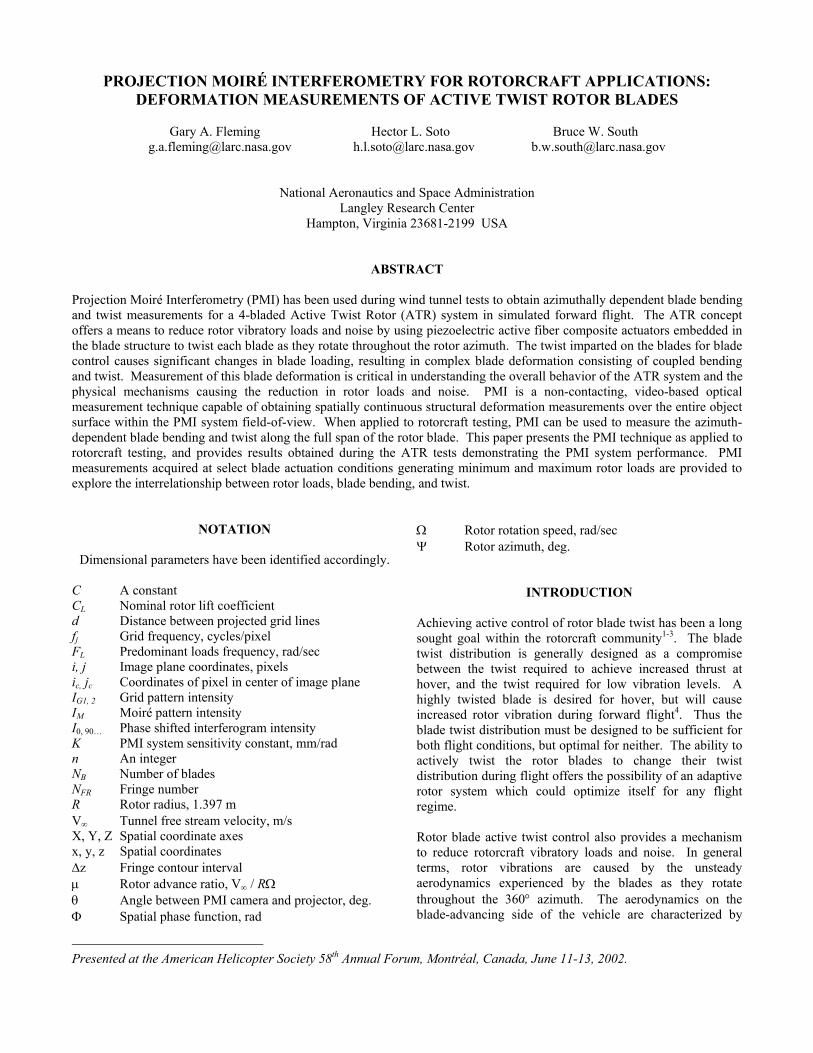
PMI Fundamentals PMI is based on the moiré effect, which occurs when two grids of similar spatial frequency are superimposed. Interference patterns occur at points where the grids intersect, producing a coarse fringe structure of lower spatial frequency than the two original grids. The process of creating moiré fringes is shown schematically in figure 1. Figure 1a shows a grid of straight parallel lines whose intensity varies cosinusoidally along the rows of the image. Mathematically, the normalized image intensity IG1 can be represented by the equation:

( ) [ ]jfjiI jG π2cos5.05.0,1 += (1) where i, j are the image row, column coordinates, and fj is the grid line frequency. Figure 1b shows the same grid as shown in figure 1a, but the intensity pattern IG2 has been distorted by the addition of a spatial phase function Φ(i, j):

( ) ( )[ ]jijfjiI jG ,2cos5.05.0,2 Φ++= π (2) The phase function used to generate the grid pattern in figure 1b is shown in figure 1c, given by:

( ) ( ) ( )222, cc jjiiCji −+−=Φ π (3) where ic, jc are the row, column coordinates of the center of the image, and C is a constant governing the phase function magnitude. The spatial phase function is smooth and continuous, but has been plotted using a 6-level palette for publication purposes. Breaks in the color palette correspond with 2πn (n = an integer) phase contours. Interfering the grids IG1 and IG2 is accomplished by taking the absolute value of their difference. The absolute value is taken because intensity is always considered a positive-valued property. Performing the interference operation produces the interferogram shown in figure 1d. The interferogram contains the desired moiré fringes, as well as high spatial

frequency artifacts of the original grids IG1 and IG2. Mathematically, the following relation is obtained:

( ) ( )

( ) ( )

Φ

Φ

+

=−=

2,sin

2,2sin

, 12

jijijfabs

IIabsjiI

j

GGM

π (4)

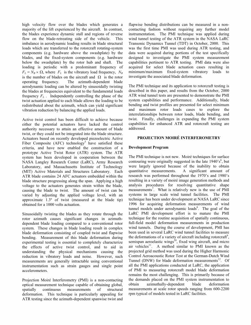
Equation (4) reaches minima for values of Φ(i, j) = 2πn, corresponding with the location of moiré fringes in the interferogram. In other words, the moiré fringes are contours of the spatial phase function with a contour interval of 2π. The moiré effect can be used to measure surface deformation by capturing images of a grid projected onto an object surface while the object is at two different positions or states of stress. To illustrate this concept, consider the PMI system shown schematically in figure 2, configured to measure the

2π4π

6π8π

10π

(a) (b) (c) (d)

Figures 1a-d: (a) Undistorted grid pattern, (b) grid pattern distorted by spatial phase function Φ(i, j) shown in (c), and (d) interferogram produced by interfering (a) and (b).

XY

Z

z-1

z 0

z+1

Projected gridintensity profile

Contour planes

Projector withRonchi ruling

CCD Camera

Projected grid lines

Grid line positionperceived by camera

d

Figure 2: Schematic of a simple PMI system

surface displacement in the Z direction. The PMI system consists of a projector whose optical axis is aligned parallel to the direction of measurement, and a CCD video camera positioned at an angle θ from the projector optical axis. A telecentric optical system is assumed for simplicity. The projector and camera lie within the X−Z plane. Assume a flat plate lying in the X−Y plane is positioned at location z 0. The projector is used to project a series of equal spaced, parallel lines onto the plate surface. A Ronchi ruling (a transmissive grating with opaque parallel lines etched at equal spacing and thickness) installed in the projector is the physical element generating the grid lines. Viewing the grid lines projected onto the plate surface with the video camera will produce an image similar to figure 1a, here referred to as a reference image. Translation of the plate in the Z direction will cause a change in the spatial locations of the grid lines observed by the camera. An image of the plate captured after the translation is here called a deformed image. Recalling equations (1) and (2), the change in observed grid line position is mathematically equivalent to distorting the grid in the reference image by a spatial phase function Φ(i, j). Geometric analysis of the schematic PMI system in figure 2 leads to the relation:

( ) ( )d

yxzji θπ tan,2, =Φ (5)

where Φ(i, j) is the spatial phase at row i, column j in the CCD camera image plane (same as defined previously for Eqns. (1) - (4)), z(x, y) is the deformation in the Z direction at point x, y on the object surface, and d is the distance between the grid lines. Interfering the reference and deformed images produces an interferogram containing moiré fringes as described in Equation (4). Again, the moiré fringes occur when Φ(i, j) = 2πn. Thus for the example PMI system in figure 2, moiré fringes will occur when:

( )θtan

, dnyxz = (6)

Equation (6) establishes that the moiré fringes define X-Y planes of constant deformation in the Z direction. Therefore

the moiré fringes in an interferogram of the test object represent contours of the object deformation along the Z axis. The fringe contour interval ∆z is:

θtandz =∆ (7)

The previous discussion has provided the background necessary to understand moiré fringe generation and how moiré fringes can be considered deformation contours. However, several notable problems remain when considering the simplified PMI system in figure 2:

a. Interferograms are directionally ambiguous, meaning the direction of deformation along the Z axis cannot be determined by the interferogram alone;

b. Deformation information between moiré fringes is indiscernible;

c. Absolute position information is lost if the test object translates through one or more contour planes; and

d. The optics used in most PMI systems are rarely telecentric.

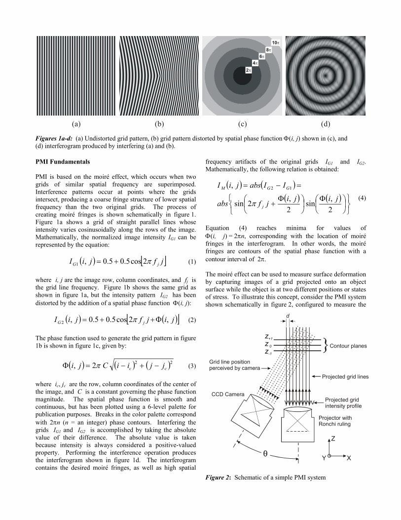
Problems (a) and (b) above can both be solved by using a technique known as phase shifting13. The goal of the phase shifting process is to determine the value of the spatial phase function Φ(i, j) at all points in the image plane. Phase shifting requires the generation of multiple interferograms, with the spatial phase of either the projected grid or a reference image incremented, or stepped, between each interferogram. Various algorithms requiring 3, 4, or 5 interferograms have been published6, but a 4-interferogram process with an incremental π/2 phase step is most common. Each of the four phase stepped interferograms must be spatially low pass filtered to eliminate the presence of high frequency artifacts caused by the interference process. Then Φ(i, j) is computed by:

( ) ( ) ( )( ) ( )

−−

=Φ −

jiIjiIjiIjiI

ji,,,,

tan,27090

18001 (8)

(a) (b) (c) (d)

Figure 3: Phase stepped interferograms, with phase step values of (a) 0°, (b) 90°, (c) 180°, and (d) 270°.

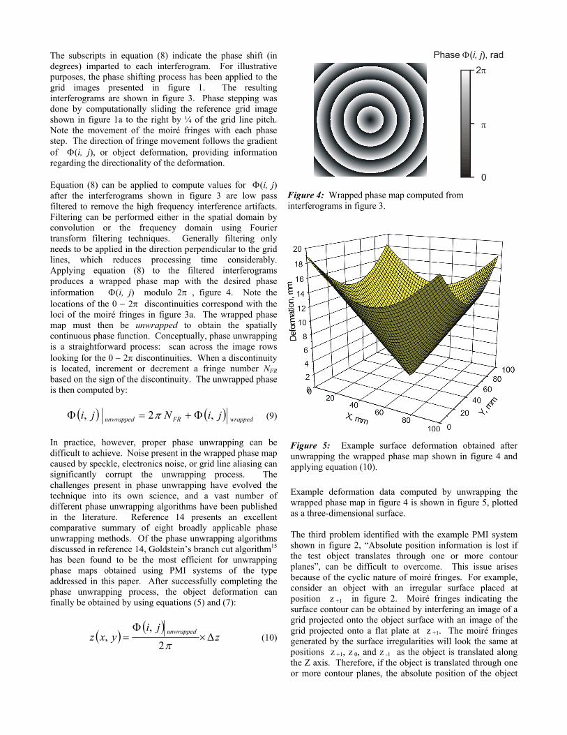
The subscripts in equation (8) indicate the phase shift (in degrees) imparted to each interferogram. For illustrative purposes, the phase shifting process has been applied to the grid images presented in figure 1. The resulting interferograms are shown in figure 3. Phase stepping was done by computationally sliding the reference grid image shown in figure 1a to the right by ¼ of the grid line pitch. Note the movement of the moiré fringes with each phase step. The direction of fringe movement follows the gradient of Φ(i, j), or object deformation, providing information regarding the directionality of the deformation. Equation (8) can be applied to compute values for Φ(i, j) after the interferograms shown in figure 3 are low pass filtered to remove the high frequency interference artifacts. Filtering can be performed either in the spatial domain by convolution or the frequency domain using Fourier transform filtering techniques. Generally filtering only needs to be applied in the direction perpendicular to the grid lines, which reduces processing time considerably. Applying equation (8) to the filtered interferograms produces a wrapped phase map with the desired phase information Φ(i, j) modulo 2π , figure 4. Note the locations of the 0 − 2π discontinuities correspond with the loci of the moiré fringes in figure 3a. The wrapped phase map must then be unwrapped to obtain the spatially continuous phase function. Conceptually, phase unwrapping is a straightforward process: scan across the image rows looking for the 0 − 2π discontinuities. When a discontinuity is located, increment or decrement a fringe number NFR based on the sign of the discontinuity. The unwrapped phase is then computed by:

( ) ( ) wrappedFRunwrapped jiNji ,2, Φ+=Φ π (9)

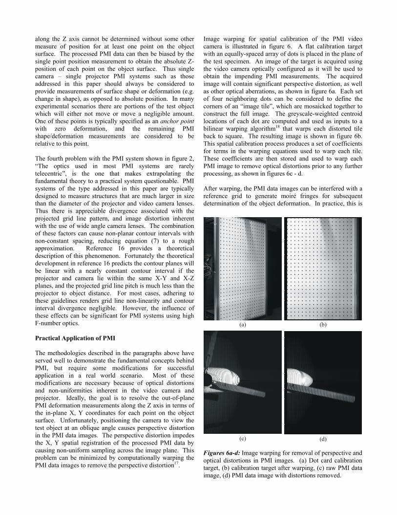
In practice, however, proper phase unwrapping can be difficult to achieve. Noise present in the wrapped phase map caused by speckle, electronics noise, or grid line aliasing can significantly corrupt the unwrapping process. The challenges present in phase unwrapping have evolved the technique into its own science, and a vast number of different phase unwrapping algorithms have been published in the literature. Reference 14 presents an excellent comparative summary of eight broadly applicable phase unwrapping methods. Of the phase unwrapping algorithms discussed in reference 14, Goldstein’s branch cut algorithm15 has been found to be the most efficient for unwrapping phase maps obtained using PMI systems of the type addressed in this paper. After successfully completing the phase unwrapping process, the object deformation can finally be obtained by using equations (5) and (7):

( )( )

zji

yxz unwrapped∆×

Φ=

π2,

, (10)

Example deformation data computed by unwrapping the wrapped phase map in figure 4 is shown in figure 5, plotted as a three-dimensional surface. The third problem identified with the example PMI system shown in figure 2, “Absolute position information is lost if the test object translates through one or more contour planes”, can be difficult to overcome. This issue arises because of the cyclic nature of moiré fringes. For example, consider an object with an irregular surface placed at position z +1 in figure 2. Moiré fringes indicating the surface contour can be obtained by interfering an image of a grid projected onto the object surface with an image of the grid projected onto a flat plate at z +1. The moiré fringes generated by the surface irregularities will look the same at positions z +1, z 0, and z -1 as the object is translated along the Z axis. Therefore, if the object is translated through one or more contour planes, the absolute position of the object

Figure 5: Example surface deformation obtained after unwrapping the wrapped phase map shown in figure 4 and applying equation (10).

0

π

2πPhase ( ), radΦ i, j

Figure 4: Wrapped phase map computed from interferograms in figure 3.

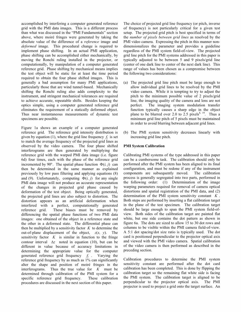
along the Z axis cannot be determined without some other measure of position for at least one point on the object surface. The processed PMI data can then be biased by the single point position measurement to obtain the absolute Z-position of each point on the object surface. Thus single camera – single projector PMI systems such as those addressed in this paper should always be considered to provide measurements of surface shape or deformation (e.g. change in shape), as opposed to absolute position. In many experimental scenarios there are portions of the test object which will either not move or move a negligible amount. One of these points is typically specified as an anchor point with zero deformation, and the remaining PMI shape/deformation measurements are considered to be relative to this point. The fourth problem with the PMI system shown in figure 2, “The optics used in most PMI systems are rarely telecentric”, is the one that makes extrapolating the fundamental theory to a practical system questionable. PMI systems of the type addressed in this paper are typically designed to measure structures that are much larger in size than the diameter of the projector and video camera lenses. Thus there is appreciable divergence associated with the projected grid line pattern, and image distortion inherent with the use of wide angle camera lenses. The combination of these factors can cause non-planar contour intervals with non-constant spacing, reducing equation (7) to a rough approximation. Reference 16 provides a theoretical description of this phenomenon. Fortunately the theoretical development in reference 16 predicts the contour planes will be linear with a nearly constant contour interval if the projector and camera lie within the same X-Y and X-Z planes, and the projected grid line pitch is much less than the projector to object distance. For most cases, adhering to these guidelines renders grid line non-linearity and contour interval divergence negligible. However, the influence of these effects can be significant for PMI systems using high F-number optics. Practical Application of PMI The methodologies described in the paragraphs above have served well to demonstrate the fundamental concepts behind PMI, but require some modifications for successful application in a real world scenario. Most of these modifications are necessary because of optical distortions and non-uniformities inherent in the video camera and projector. Ideally, the goal is to resolve the out-of-plane PMI deformation measurements along the Z axis in terms of the in-plane X, Y coordinates for each point on the object surface. Unfortunately, positioning the camera to view the test object at an oblique angle causes perspective distortion in the PMI data images. The perspective distortion impedes the X, Y spatial registration of the processed PMI data by causing non-uniform sampling across the image plane. This problem can be minimized by computationally warping the PMI data images to remove the perspective distortion17.

Image warping for spatial calibration of the PMI video camera is illustrated in figure 6. A flat calibration target with an equally-spaced array of dots is placed in the plane of the test specimen. An image of the target is acquired using the video camera optically configured as it will be used to obtain the impending PMI measurements. The acquired image will contain significant perspective distortion, as well as other optical aberrations, as shown in figure 6a. Each set of four neighboring dots can be considered to define the corners of an “image tile”, which are mosaicked together to construct the full image. The greyscale-weighted centroid locations of each dot are computed and used as inputs to a bilinear warping algorithm18 that warps each distorted tile back to square. The resulting image is shown in figure 6b. This spatial calibration process produces a set of coefficients for terms in the warping equations used to warp each tile. These coefficients are then stored and used to warp each PMI image to remove optical distortions prior to any further processing, as shown in figures 6c - d. After warping, the PMI data images can be interfered with a reference grid to generate moiré fringes for subsequent determination of the object deformation. In practice, this is

(a) (b)

(c) (d)

Figures 6a-d: Image warping for removal of perspective and optical distortions in PMI images. (a) Dot card calibration target, (b) calibration target after warping, (c) raw PMI data image, (d) PMI data image with distortions removed.

accomplished by interfering a computer generated reference grid with the PMI data images. This is a different process than what was discussed in the “PMI Fundamentals” section above, where moiré fringes were generated by taking the absolute value of the difference of a reference image and deformed image. This procedural change is required to implement phase shifting. In an actual PMI application, phase shifting can be accomplished either mechanically, by moving the Ronchi ruling installed in the projector, or computationally, by manipulation of a computer generated reference grid. Phase shifting by mechanical means implies the test object will be static for at least the time period required to obtain the four phase shifted images. This is generally a bad assumption for many PMI applications, particularly those that are wind tunnel-based. Mechanically shifting the Ronchi ruling also adds complexity to the instrument, and stringent mechanical tolerances are required to achieve accurate, repeatable shifts. Besides keeping the optics simple, using a computer generated reference grid eliminates the requirement of a statically deformed object. Thus near instantaneous measurements of dynamic test specimens are possible. Figure 1a shows an example of a computer generated reference grid. The reference grid intensity distribution is given by equation (1), where the grid line frequency fj is set to match the average frequency of the projected grid lines as observed by the video camera. The four phase shifted interferograms are then generated by multiplying the reference grid with the warped PMI data image (i.e. figure 6d) four times, each with the phase of the reference grid incremented by 90°. The spatial phase function Φ(i, j) can then be determined in the same manner as explained previously by low pass filtering and applying equations (8) and (9). Unfortunately, computing Φ(i, j) for any single PMI data image will not produce an accurate representation of the changes in projected grid phase caused by deformation of the test object. Being optically generated, the projected grid lines are also subject to distortion. The distortion appears as an artificial deformation when interfered with a perfect, computationally generated reference grid. These biases must be removed by differencing the spatial phase functions of two PMI data images: one obtained of the object in a reference state and the other in a deformed state. The differential phase can then be multiplied by a sensitivity factor K to determine the out-of-plane displacement of the object, z(x, y). The sensitivity factor K is similar in function to the fringe contour interval ∆z noted in equation (10), but can be different in value because of accuracy limitations in determining the appropriate value for the computer generated reference grid frequency fj . Varying the reference grid frequency by as much as 1% can significantly alter the shape and position of moiré fringes in the interferograms. Thus the true value for K must be determined through calibration of the PMI system for a specific reference grid frequency. These calibration procedures are discussed in the next section of this paper.

The choice of projected grid line frequency (or pitch, inverse of frequency) is not particularly critical for a given test setup. The projected grid pitch is best specified in terms of the number of pixels between grid lines as resolved by the PMI video camera. Expressing the pitch in this manner non-dimensionalizes the parameter and provides a guideline regardless of the PMI system field-of-view. The projected grid line pitch for the PMI systems addressed in this paper is typically adjusted to be between 5 and 9 pixels/grid line (center of one dark line to center of the next dark line). This range of values has been chosen as a compromise between the following two considerations: (a) The projected grid line pitch must be large enough to

allow individual grid lines to be resolved by the PMI video camera. While it is tempting to try to adjust the pitch to the minimum possible value of 2 pixels/grid line, the imaging quality of the camera and lens are not perfect. The imaging system modulation transfer function typically causes a sharp edge in the object plane to be blurred over 2.0 to 2.5 pixels8, 19. Thus a minimum grid line pitch of 5 pixels must be maintained in order to avoid blurring between adjacent grid lines.

(b) The PMI system sensitivity decreases linearly with

increasing grid line pitch. PMI System Calibration Calibrating PMI systems of the type addressed in this paper can be a cumbersome task. The calibration should only be performed after the PMI system has been aligned to its final configuration, and must be redone if any of the instrument components are subsequently moved. The calibration process is generally segregated into two parts, performed in the following order: (1) Determination of the image warping parameters required for removal of camera optical distortions and spatial registration of the PMI data, and (2) determination of the PMI system sensitivity constant K . Both steps are performed by inserting a flat calibration target in the plane of the test specimen. The calibration target should be large enough to span the PMI system field-of-view. Both sides of the calibration target are painted flat white, but one side contains the dot pattern as shown in figure 6a. The dots are sized to allow 15 to 30 dot rows and columns to be visible within the PMI camera field-of-view. A 5:1 dot spacing/dot size ratio is typically used. The dot card is positioned perpendicular to the projector optical axis and viewed with the PMI video camera. Spatial calibration of the video camera is then performed as described in the preceding section. Calibration procedures to determine the PMI system sensitivity constant are performed after the dot card calibration has been completed. This is done by flipping the calibration target so the remaining flat white side is facing the PMI system. The calibration target is aligned to be perpendicular to the projector optical axis. The PMI projector is used to project a grid onto the target surface. An

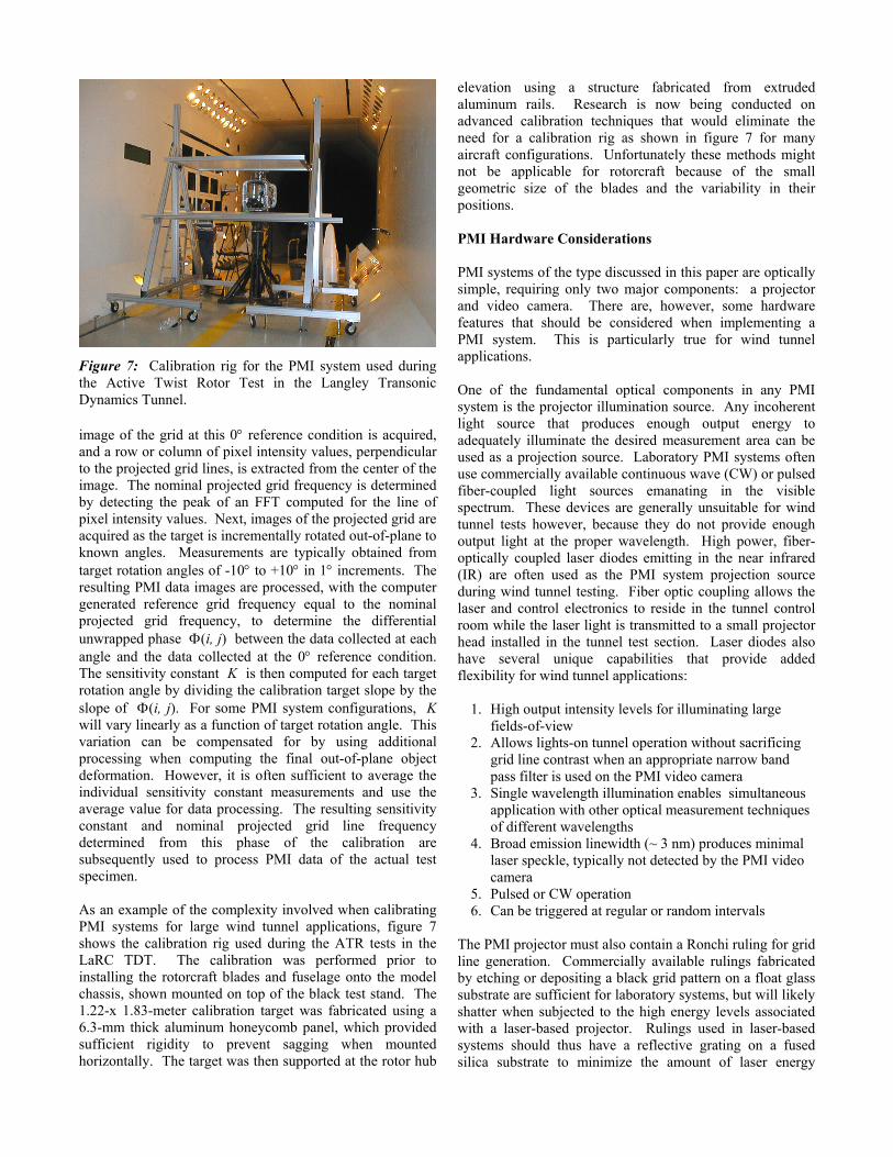
image of the grid at this 0° reference condition is acquired, and a row or column of pixel intensity values, perpendicular to the projected grid lines, is extracted from the center of the image. The nominal projected grid frequency is determined by detecting the peak of an FFT computed for the line of pixel intensity values. Next, images of the projected grid are acquired as the target is incrementally rotated out-of-plane to known angles. Measurements are typically obtained from target rotation angles of -10° to +10° in 1° increments. The resulting PMI data images are processed, with the computer generated reference grid frequency equal to the nominal projected grid frequency, to determine the differential unwrapped phase Φ(i, j) between the data collected at each angle and the data collected at the 0° reference condition. The sensitivity constant K is then computed for each target rotation angle by dividing the calibration target slope by the slope of Φ(i, j). For some PMI system configurations, K will vary linearly as a function of target rotation angle. This variation can be compensated for by using additional processing when computing the final out-of-plane object deformation. However, it is often sufficient to average the individual sensitivity constant measurements and use the average value for data processing. The resulting sensitivity constant and nominal projected grid line frequency determined from this phase of the calibration are subsequently used to process PMI data of the actual test specimen. As an example of the complexity involved when calibrating PMI systems for large wind tunnel applications, figure 7 shows the calibration rig used during the ATR tests in the LaRC TDT. The calibration was performed prior to installing the rotorcraft blades and fuselage onto the model chassis, shown mounted on top of the black test stand. The 1.22-x 1.83-meter calibration target was fabricated using a 6.3-mm thick aluminum honeycomb panel, which provided sufficient rigidity to prevent sagging when mounted horizontally. The target was then supported at the rotor hub

elevation using a structure fabricated from extruded aluminum rails. Research is now being conducted on advanced calibration techniques that would eliminate the need for a calibration rig as shown in figure 7 for many aircraft configurations. Unfortunately these methods might not be applicable for rotorcraft because of the small geometric size of the blades and the variability in their positions. PMI Hardware Considerations PMI systems of the type discussed in this paper are optically simple, requiring only two major components: a projector and video camera. There are, however, some hardware features that should be considered when implementing a PMI system. This is particularly true for wind tunnel applications. One of the fundamental optical components in any PMI system is the projector illumination source. Any incoherent light source that produces enough output energy to adequately illuminate the desired measurement area can be used as a projection source. Laboratory PMI systems often use commercially available continuous wave (CW) or pulsed fiber-coupled light sources emanating in the visible spectrum. These devices are generally unsuitable for wind tunnel tests however, because they do not provide enough output light at the proper wavelength. High power, fiber-optically coupled laser diodes emitting in the near infrared (IR) are often used as the PMI system projection source during wind tunnel testing. Fiber optic coupling allows the laser and control electronics to reside in the tunnel control room while the laser light is transmitted to a small projector head installed in the tunnel test section. Laser diodes also have several unique capabilities that provide added flexibility for wind tunnel applications:

1. High output intensity levels for illuminating large fields-of-view

2. Allows lights-on tunnel operation without sacrificing grid line contrast when an appropriate narrow band pass filter is used on the PMI video camera

3. Single wavelength illumination enables simultaneous application with other optical measurement techniques of different wavelengths

4. Broad emission linewidth (~ 3 nm) produces minimal laser speckle, typically not detected by the PMI video camera

5. Pulsed or CW operation 6. Can be triggered at regular or random intervals

The PMI projector must also contain a Ronchi ruling for grid line generation. Commercially available rulings fabricated by etching or depositing a black grid pattern on a float glass substrate are sufficient for laboratory systems, but will likely shatter when subjected to the high energy levels associated with a laser-based projector. Rulings used in laser-based systems should thus have a reflective grating on a fused silica substrate to minimize the amount of laser energy

Figure 7: Calibration rig for the PMI system used during the Active Twist Rotor Test in the Langley Transonic Dynamics Tunnel.

absorbed into the optic. The ruling pitch varies by application, but typically ranges from 8 to 24 line pairs/mm. Most commercially available monochrome CCD video cameras are suitable for use in PMI systems. The imager should provide at least 640-x 480 pixel resolution, and progressive scan technology is desirable in order to avoid interlacing effects. Cameras with asynchronous reset offer triggering capabilities which are critical in capturing near instantaneous measurements of transient objects (e.g. rotor blades). Cameras having increased sensitivity in the near IR are beneficial for laser-based PMI systems, except caution must be exercised because the enhanced sensitivity often comes at the sacrifice of increased camera noise. High quality video lenses can be used for both the projector and video camera. Several manufacturers offer lenses that are coated for transmission in the near IR, which offer slight improvements in optical throughput for laser-based PMI systems. Zoom lenses are suitable for laboratory use, but more rugged fixed focal length lenses with lockdown screws are recommended for PMI testing in wind tunnels. A final hardware consideration regards the surface finish of the object being measured. PMI measurements can be obtained on any surface that provides enough diffuse scattered light to make the projected grid visible to the PMI system video camera. Therefore surface treatment is not necessary for most solid surfaces. Very dark surfaces, or highly polished metallic surfaces that reflect light specularly, may require painting. PMI Measurement Accuracy and Resolution The out-of-plane deformation measurement resolution of a PMI system is primarily dependent on the video camera field-of-view, camera and projector optical modulation transfer functions, and illumination/observation angles. As a conservative rule-of-thumb, the out-of-plane deformation measurement accuracy and resolution of a PMI system can be approximated at 1/1500 and 1/2500 of the field-of-view respectively. Deformation measurement resolutions better than 0.05-mm have been attained with conventional laboratory systems using 640-x 480-pixel video cameras with a 300-x 300-mm field-of-view. Absolute deformation measurement accuracies better than 0.15-mm over a 50-mm range of deformation have been achieved for similar laboratory systems. Wind tunnel-based PMI systems generally suffer somewhat degraded accuracy and performance specifications compared to their laboratory counterparts because of the often harsh wind tunnel environment. However, a wind tunnel-based PMI system with a 1.2-x 1.2-meter field-of-view has been shown to demonstrate 0.75-mm measurement accuracy10, adhering to the rule-of-thumb approximation.

OVERVIEW OF THE ACTIVE TWIST ROTOR WIND TUNNEL TEST

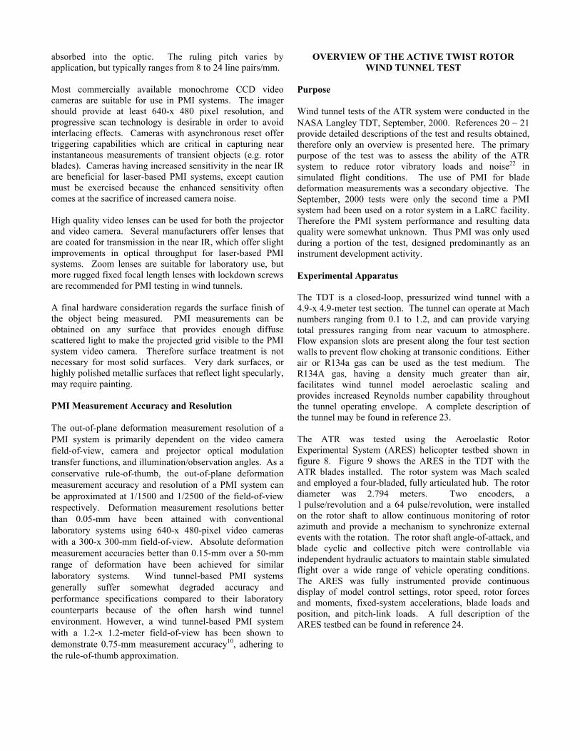
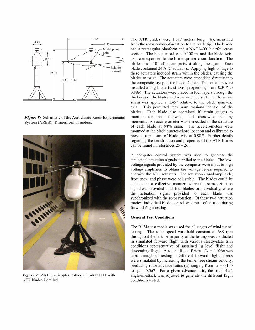
Purpose Wind tunnel tests of the ATR system were conducted in the NASA Langley TDT, September, 2000. References 20 − 21 provide detailed descriptions of the test and results obtained, therefore only an overview is presented here. The primary purpose of the test was to assess the ability of the ATR system to reduce rotor vibratory loads and noise22 in simulated flight conditions. The use of PMI for blade deformation measurements was a secondary objective. The September, 2000 tests were only the second time a PMI system had been used on a rotor system in a LaRC facility. Therefore the PMI system performance and resulting data quality were somewhat unknown. Thus PMI was only used during a portion of the test, designed predominantly as an instrument development activity. Experimental Apparatus The TDT is a closed-loop, pressurized wind tunnel with a 4.9-x 4.9-meter test section. The tunnel can operate at Mach numbers ranging from 0.1 to 1.2, and can provide varying total pressures ranging from near vacuum to atmosphere. Flow expansion slots are present along the four test section walls to prevent flow choking at transonic conditions. Either air or R134a gas can be used as the test medium. The R134A gas, having a density much greater than air, facilitates wind tunnel model aeroelastic scaling and provides increased Reynolds number capability throughout the tunnel operating envelope. A complete description of the tunnel may be found in reference 23. The ATR was tested using the Aeroelastic Rotor Experimental System (ARES) helicopter testbed shown in figure 8. Figure 9 shows the ARES in the TDT with the ATR blades installed. The rotor system was Mach scaled and employed a four-bladed, fully articulated hub. The rotor diameter was 2.794 meters. Two encoders, a 1 pulse/revolution and a 64 pulse/revolution, were installed on the rotor shaft to allow continuous monitoring of rotor azimuth and provide a mechanism to synchronize external events with the rotation. The rotor shaft angle-of-attack, and blade cyclic and collective pitch were controllable via independent hydraulic actuators to maintain stable simulated flight over a wide range of vehicle operating conditions. The ARES was fully instrumented provide continuous display of model control settings, rotor speed, rotor forces and moments, fixed-system accelerations, blade loads and position, and pitch-link loads. A full description of the ARES testbed can be found in reference 24.

The ATR blades were 1.397 meters long (R), measured from the rotor center-of-rotation to the blade tip. The blades had a rectangular planform and a NACA-0012 airfoil cross section. The blade chord was 0.108 m, and the blade twist axis corresponded to the blade quarter-chord location. The blades had -10° of linear pretwist along the span. Each blade contained 24 AFC actuators. Applying high voltage to these actuators induced strain within the blades, causing the blades to twist. The actuators were embedded directly into the composite layup of the blade D-spar. The actuators were installed along blade twist axis, progressing from 0.30R to 0.98R. The actuators were placed in four layers through the thickness of the blades and were oriented such that the active strain was applied at ±45° relative to the blade spanwise axis. This permitted maximum torsional control of the blades. Each blade also contained 10 strain gauges to monitor torsional, flapwise, and chordwise bending moments. An accelerometer was embedded in the structure of each blade at 98% span. The accelerometers were mounted at the blade quarter-chord location and calibrated to provide a measure of blade twist at 0.98R. Further details regarding the construction and properties of the ATR blades can be found in references 25 – 26. A computer control system was used to generate the sinusoidal actuation signals supplied to the blades. The low-voltage signals provided by the computer were input to high voltage amplifiers to obtain the voltage levels required to energize the AFC actuators. The actuation signal amplitude, frequency, and phase were adjustable. The blades could be actuated in a collective manner, where the same actuation signal was provided to all four blades, or individually, where the actuation signal provided to each blade was synchronized with the rotor rotation. Of these two actuation modes, individual blade control was most often used during forward flight testing. General Test Conditions The R134a test media was used for all stages of wind tunnel testing. The rotor speed was held constant at 688 rpm throughout the test. A majority of the testing was conducted in simulated forward flight with various steady-state trim conditions representative of sustained 1g level flight and descending flight. A rotor lift coefficient CL = 0.0066 was used throughout testing. Different forward flight speeds were simulated by increasing the tunnel free stream velocity, producing rotor advance ratios (µ) ranging from µ = 0.140 to µ = 0.367. For a given advance ratio, the rotor shaft angle-of-attack was adjusted to generate the different flight conditions tested.

Figure 9: ARES helicopter testbed in LaRC TDT with ATR blades installed.

Model pivotpoint

Balancecentroid

2.55

1.52

1.841.92

2.37

0.62

0.41

Figure 8: Schematic of the Aeroelastic Rotor Experimental System (ARES). Dimensions in meters.

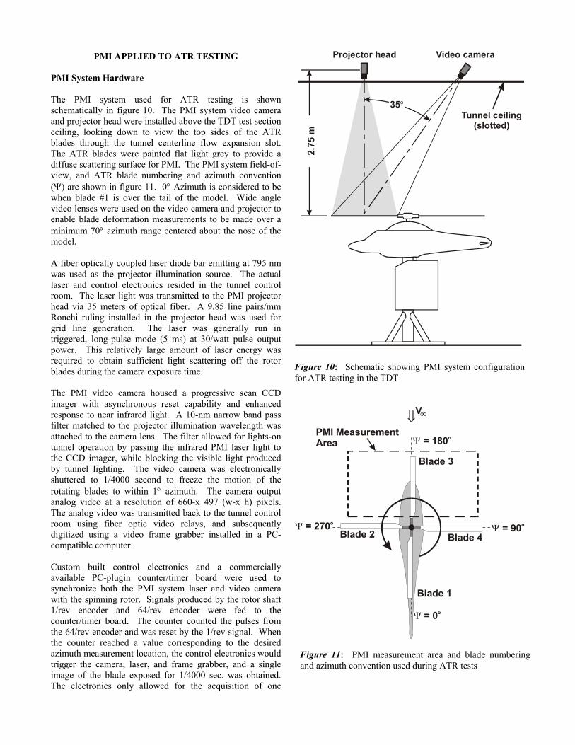
PMI APPLIED TO ATR TESTING PMI System Hardware The PMI system used for ATR testing is shown schematically in figure 10. The PMI system video camera and projector head were installed above the TDT test section ceiling, looking down to view the top sides of the ATR blades through the tunnel centerline flow expansion slot. The ATR blades were painted flat light grey to provide a diffuse scattering surface for PMI. The PMI system field-of-view, and ATR blade numbering and azimuth convention (Ψ) are shown in figure 11. 0° Azimuth is considered to be when blade #1 is over the tail of the model. Wide angle video lenses were used on the video camera and projector to enable blade deformation measurements to be made over a minimum 70° azimuth range centered about the nose of the model. A fiber optically coupled laser diode bar emitting at 795 nm was used as the projector illumination source. The actual laser and control electronics resided in the tunnel control room. The laser light was transmitted to the PMI projector head via 35 meters of optical fiber. A 9.85 line pairs/mm Ronchi ruling installed in the projector head was used for grid line generation. The laser was generally run in triggered, long-pulse mode (5 ms) at 30/watt pulse output power. This relatively large amount of laser energy was required to obtain sufficient light scattering off the rotor blades during the camera exposure time. The PMI video camera housed a progressive scan CCD imager with asynchronous reset capability and enhanced response to near infrared light. A 10-nm narrow band pass filter matched to the projector illumination wavelength was attached to the camera lens. The filter allowed for lights-on tunnel operation by passing the infrared PMI laser light to the CCD imager, while blocking the visible light produced by tunnel lighting. The video camera was electronically shuttered to 1/4000 second to freeze the motion of the rotating blades to within 1° azimuth. The camera output analog video at a resolution of 660-x 497 (w-x h) pixels. The analog video was transmitted back to the tunnel control room using fiber optic video relays, and subsequently digitized using a video frame grabber installed in a PC-compatible computer. Custom built control electronics and a commercially available PC-plugin counter/timer board were used to synchronize both the PMI system laser and video camera with the spinning rotor. Signals produced by the rotor shaft 1/rev encoder and 64/rev encoder were fed to the counter/timer board. The counter counted the pulses from the 64/rev encoder and was reset by the 1/rev signal. When the counter reached a value corresponding to the desired azimuth measurement location, the control electronics would trigger the camera, laser, and frame grabber, and a single image of the blade exposed for 1/4000 sec. was obtained. The electronics only allowed for the acquisition of one

Video camera

Tunnel ceiling(slotted)

Projector head

2.75

m

35 °

Figure 10: Schematic showing PMI system configuration for ATR testing in the TDT

Blade 1

Blade 2

Blade 3

PMI MeasurementArea

Blade 4

Ψ = 0o

Ψ = 90oΨ = 270o

Ψ = 180o

V

Figure 11: PMI measurement area and blade numbering and azimuth convention used during ATR tests

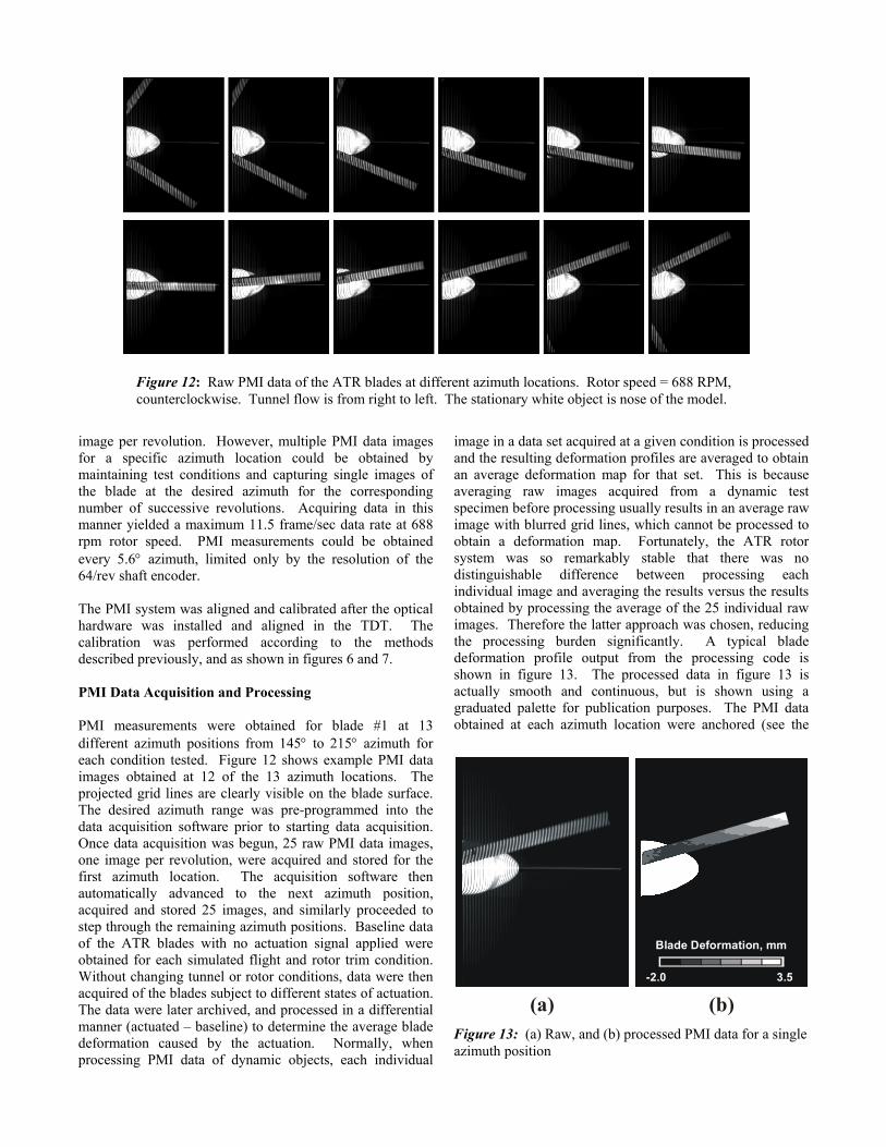
image per revolution. However, multiple PMI data images for a specific azimuth location could be obtained by maintaining test conditions and capturing single images of the blade at the desired azimuth for the corresponding number of successive revolutions. Acquiring data in this manner yielded a maximum 11.5 frame/sec data rate at 688 rpm rotor speed. PMI measurements could be obtained every 5.6° azimuth, limited only by the resolution of the 64/rev shaft encoder. The PMI system was aligned and calibrated after the optical hardware was installed and aligned in the TDT. The calibration was performed according to the methods described previously, and as shown in figures 6 and 7. PMI Data Acquisition and Processing PMI measurements were obtained for blade #1 at 13 different azimuth positions from 145° to 215° azimuth for each condition tested. Figure 12 shows example PMI data images obtained at 12 of the 13 azimuth locations. The projected grid lines are clearly visible on the blade surface. The desired azimuth range was pre-programmed into the data acquisition software prior to starting data acquisition. Once data acquisition was begun, 25 raw PMI data images, one image per revolution, were acquired and stored for the first azimuth location. The acquisition software then automatically advanced to the next azimuth position, acquired and stored 25 images, and similarly proceeded to step through the remaining azimuth positions. Baseline data of the ATR blades with no actuation signal applied were obtained for each simulated flight and rotor trim condition. Without changing tunnel or rotor conditions, data were then acquired of the blades subject to different states of actuation. The data were later archived, and processed in a differential manner (actuated – baseline) to determine the average blade deformation caused by the actuation. Normally, when processing PMI data of dynamic objects, each individual

image in a data set acquired at a given condition is processed and the resulting deformation profiles are averaged to obtain an average deformation map for that set. This is because averaging raw images acquired from a dynamic test specimen before processing usually results in an average raw image with blurred grid lines, which cannot be processed to obtain a deformation map. Fortunately, the ATR rotor system was so remarkably stable that there was no distinguishable difference between processing each individual image and averaging the results versus the results obtained by processing the average of the 25 individual raw images. Therefore the latter approach was chosen, reducing the processing burden significantly. A typical blade deformation profile output from the processing code is shown in figure 13. The processed data in figure 13 is actually smooth and continuous, but is shown using a graduated palette for publication purposes. The PMI data obtained at each azimuth location were anchored (see the

Figure 12: Raw PMI data of the ATR blades at different azimuth locations. Rotor speed = 688 RPM, counterclockwise. Tunnel flow is from right to left. The stationary white object is nose of the model.

Figure 13: (a) Raw, and (b) processed PMI data for a single azimuth position

(a) (b)-2.0 3.5

Blade Deformation, mm

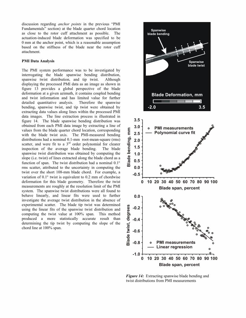
discussion regarding anchor points in the previous “PMI Fundamentals” section) at the blade quarter chord location as close to the rotor cuff attachment as possible. The actuation-induced blade deformation was specified to be 0 mm at the anchor point, which is a reasonable assumption based on the stiffness of the blade near the rotor cuff attachment. PMI Data Analysis The PMI system performance was to be investigated by interrogating the blade spanwise bending distribution, spanwise twist distribution, and tip twist. Although displaying the processed PMI data as an image as shown in figure 13 provides a global perspective of the blade deformation at a given azimuth, it contains coupled bending and twist information and has limited value for further detailed quantitative analysis. Therefore the spanwise bending, spanwise twist, and tip twist were obtained by extracting data values along lines within the processed PMI data images. The line extraction process is illustrated in figure 14. The blade spanwise bending distribution was obtained from each PMI data image by extracting a line of values from the blade quarter chord location, corresponding with the blade twist axis. The PMI-measured bending distributions had a nominal 0.1-mm root-mean-square (rms) scatter, and were fit to a 3rd order polynomial for clearer inspection of the average blade bending. The blade spanwise twist distribution was obtained by computing the slope (i.e. twist) of lines extracted along the blade chord as a function of span. The twist distribution had a nominal 0.1° rms scatter, attributed to the uncertainty in computing the twist over the short 108-mm blade chord. For example, a variation of 0.1° twist is equivalent to 0.2 mm of chordwise deformation for this blade geometry. Therefore the twist measurements are roughly at the resolution limit of the PMI system. The spanwise twist distributions were all found to behave linearly, and linear fits were used to further investigate the average twist distribution in the absence of experimental scatter. The blade tip twist was determined using the linear fits of the spanwise twist distribution and computing the twist value at 100% span. This method produced a more statistically accurate result than determining the tip twist by computing the slope of the chord line at 100% span.

Figure 14: Extracting spanwise blade bending and twist distributions from PMI measurements

0 10 20 30 40 50 60 70 80 90 100

-0.50.00.51.01.52.02.53.03.5

Blade span, percent

Bla

de b

endi

ng, m

m PMI measurementsPolynomial curve fit

0 10 20 30 40 50 60 70 80 90 100Blade span, percent

Bla

de tw

ist,

degr

ees

PMI measurementsLinear regression

-1.0

-0.8

-0.6

-0.4

-0.2

0.0

Spanwiseblade twist

Spanwiseblade bending

-2.0 3.5

Blade Deformation, mm

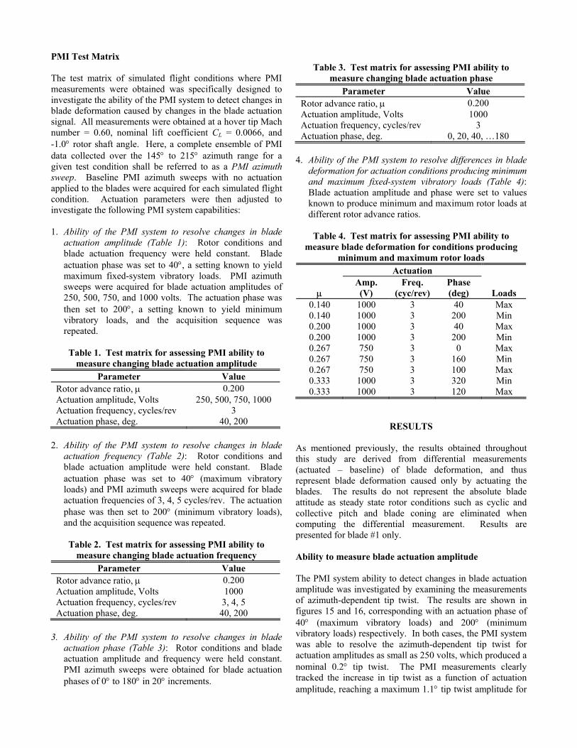
PMI Test Matrix The test matrix of simulated flight conditions where PMI measurements were obtained was specifically designed to investigate the ability of the PMI system to detect changes in blade deformation caused by changes in the blade actuation signal. All measurements were obtained at a hover tip Mach number = 0.60, nominal lift coefficient CL = 0.0066, and -1.0° rotor shaft angle. Here, a complete ensemble of PMI data collected over the 145° to 215° azimuth range for a given test condition shall be referred to as a PMI azimuth sweep. Baseline PMI azimuth sweeps with no actuation applied to the blades were acquired for each simulated flight condition. Actuation parameters were then adjusted to investigate the following PMI system capabilities: 1. Ability of the PMI system to resolve changes in blade

actuation amplitude (Table 1): Rotor conditions and blade actuation frequency were held constant. Blade actuation phase was set to 40°, a setting known to yield maximum fixed-system vibratory loads. PMI azimuth sweeps were acquired for blade actuation amplitudes of 250, 500, 750, and 1000 volts. The actuation phase was then set to 200°, a setting known to yield minimum vibratory loads, and the acquisition sequence was repeated.

Table 1. Test matrix for assessing PMI ability to

measure changing blade actuation amplitude Parameter Value

Rotor advance ratio, µ 0.200 Actuation amplitude, Volts 250, 500, 750, 1000 Actuation frequency, cycles/rev 3 Actuation phase, deg. 40, 200

2. Ability of the PMI system to resolve changes in blade

actuation frequency (Table 2): Rotor conditions and blade actuation amplitude were held constant. Blade actuation phase was set to 40° (maximum vibratory loads) and PMI azimuth sweeps were acquired for blade actuation frequencies of 3, 4, 5 cycles/rev. The actuation phase was then set to 200° (minimum vibratory loads), and the acquisition sequence was repeated.

Table 2. Test matrix for assessing PMI ability to

measure changing blade actuation frequency Parameter Value

Rotor advance ratio, µ 0.200 Actuation amplitude, Volts 1000 Actuation frequency, cycles/rev 3, 4, 5 Actuation phase, deg. 40, 200

3. Ability of the PMI system to resolve changes in blade

actuation phase (Table 3): Rotor conditions and blade actuation amplitude and frequency were held constant. PMI azimuth sweeps were obtained for blade actuation phases of 0° to 180° in 20° increments.

Table 3. Test matrix for assessing PMI ability to

measure changing blade actuation phase Parameter Value

Rotor advance ratio, µ 0.200 Actuation amplitude, Volts 1000 Actuation frequency, cycles/rev 3 Actuation phase, deg. 0, 20, 40, …180

4. Ability of the PMI system to resolve differences in blade

deformation for actuation conditions producing minimum and maximum fixed-system vibratory loads (Table 4): Blade actuation amplitude and phase were set to values known to produce minimum and maximum rotor loads at different rotor advance ratios.

Table 4. Test matrix for assessing PMI ability to

measure blade deformation for conditions producing minimum and maximum rotor loads

Actuation

µ Amp. (V)

Freq. (cyc/rev)

Phase (deg) Loads

0.140 1000 3 40 Max 0.140 1000 3 200 Min 0.200 1000 3 40 Max 0.200 1000 3 200 Min 0.267 750 3 0 Max 0.267 750 3 160 Min 0.267 750 3 100 Max 0.333 1000 3 320 Min 0.333 1000 3 120 Max

RESULTS As mentioned previously, the results obtained throughout this study are derived from differential measurements (actuated – baseline) of blade deformation, and thus represent blade deformation caused only by actuating the blades. The results do not represent the absolute blade attitude as steady state rotor conditions such as cyclic and collective pitch and blade coning are eliminated when computing the differential measurement. Results are presented for blade #1 only. Ability to measure blade actuation amplitude The PMI system ability to detect changes in blade actuation amplitude was investigated by examining the measurements of azimuth-dependent tip twist. The results are shown in figures 15 and 16, corresponding with an actuation phase of 40° (maximum vibratory loads) and 200° (minimum vibratory loads) respectively. In both cases, the PMI system was able to resolve the azimuth-dependent tip twist for actuation amplitudes as small as 250 volts, which produced a nominal 0.2° tip twist. The PMI measurements clearly tracked the increase in tip twist as a function of actuation amplitude, reaching a maximum 1.1° tip twist amplitude for

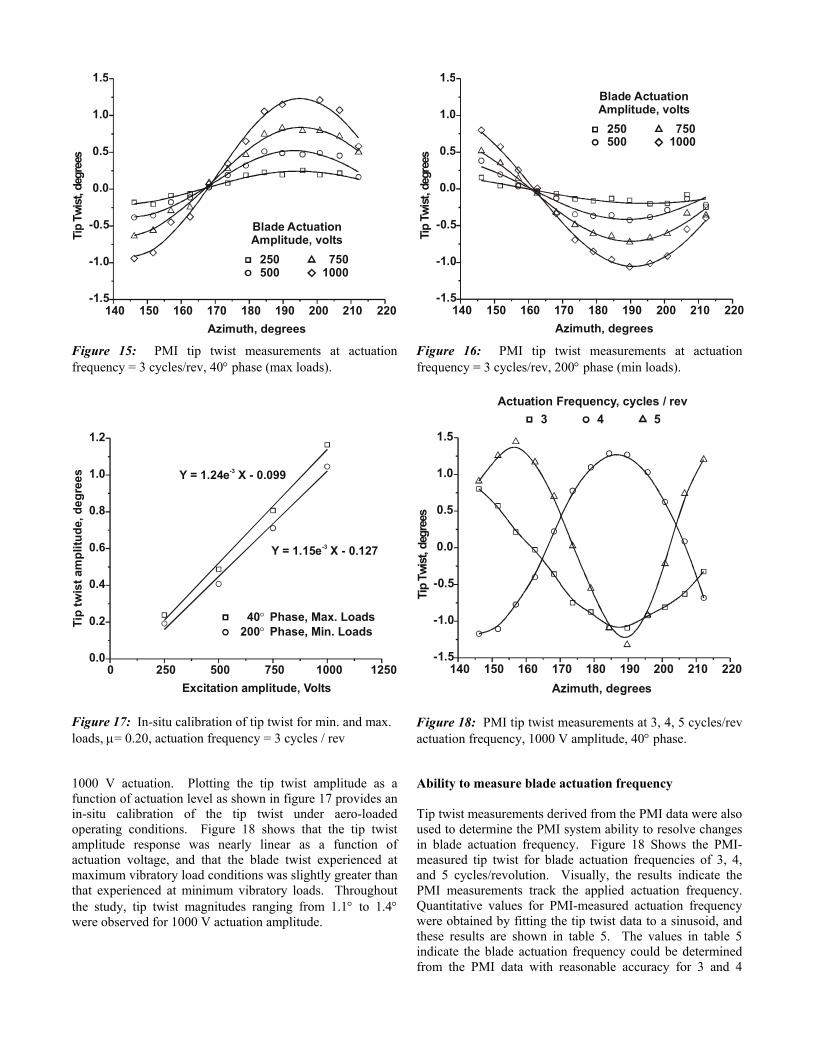
1000 V actuation. Plotting the tip twist amplitude as a function of actuation level as shown in figure 17 provides an in-situ calibration of the tip twist under aero-loaded operating conditions. Figure 18 shows that the tip twist amplitude response was nearly linear as a function of actuation voltage, and that the blade twist experienced at maximum vibratory load conditions was slightly greater than that experienced at minimum vibratory loads. Throughout the study, tip twist magnitudes ranging from 1.1° to 1.4° were observed for 1000 V actuation amplitude.

Ability to measure blade actuation frequency Tip twist measurements derived from the PMI data were also used to determine the PMI system ability to resolve changes in blade actuation frequency. Figure 18 Shows the PMI-measured tip twist for blade actuation frequencies of 3, 4, and 5 cycles/revolution. Visually, the results indicate the PMI measurements track the applied actuation frequency. Quantitative values for PMI-measured actuation frequency were obtained by fitting the tip twist data to a sinusoid, and these results are shown in table 5. The values in table 5 indicate the blade actuation frequency could be determined from the PMI data with reasonable accuracy for 3 and 4

140 150 160 170 180 190 200 210 220-1.5

-1.0

-0.5

0.0

0.5

1.0

1.5Ti

pTw

ist,

degr

ees

Azimuth, degrees

Blade ActuationAmplitude, volts

250 500

750 1000

Figure 15: PMI tip twist measurements at actuation frequency = 3 cycles/rev, 40° phase (max loads).

140 150 160 170 180 190 200 210 220-1.5

-1.0

-0.5

0.0

0.5

1.0

1.5

Tip

Twist

,deg

rees

Azimuth, degrees

Blade ActuationAmplitude, volts

250 500

750 1000

Figure 16: PMI tip twist measurements at actuation frequency = 3 cycles/rev, 200° phase (min loads).

0 250 500 750 1000 12500.0

0.2

0.4

0.6

0.8

1.0

1.2

Y = 1.24e X - 0.099-3

Excitation amplitude, Volts

40° Phase, Max. Loads 200° Phase, Min. LoadsTi

p tw

ist a

mpl

itude

, deg

rees

Y = 1.15e X - 0.127-3

Figure 17: In-situ calibration of tip twist for min. and max. loads, µ= 0.20, actuation frequency = 3 cycles / rev

140 150 160 170 180 190 200 210 220-1.5

-1.0

-0.5

0.0

0.5

1.0

1.5Ti

pTw

ist,

degr

ees

Azimuth, degrees

Actuation Frequency, cycles / rev 3 4 5

Figure 18: PMI tip twist measurements at 3, 4, 5 cycles/rev actuation frequency, 1000 V amplitude, 40° phase.

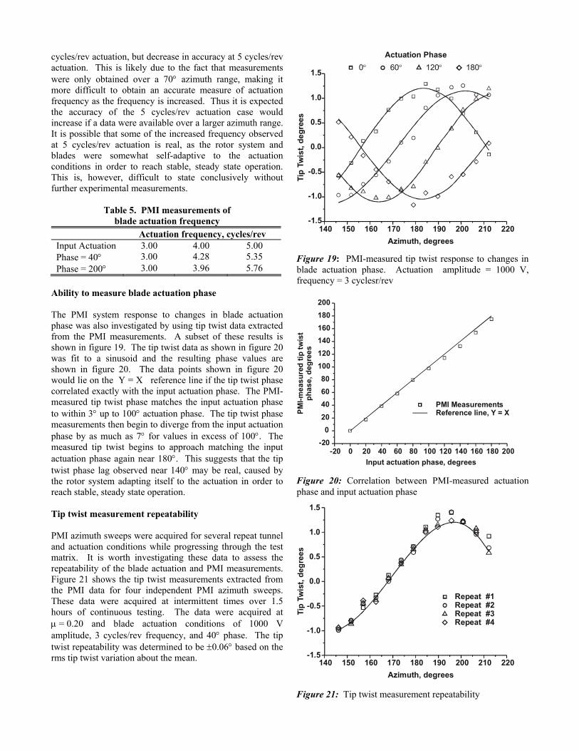
cycles/rev actuation, but decrease in accuracy at 5 cycles/rev actuation. This is likely due to the fact that measurements were only obtained over a 70° azimuth range, making it more difficult to obtain an accurate measure of actuation frequency as the frequency is increased. Thus it is expected the accuracy of the 5 cycles/rev actuation case would increase if a data were available over a larger azimuth range. It is possible that some of the increased frequency observed at 5 cycles/rev actuation is real, as the rotor system and blades were somewhat self-adaptive to the actuation conditions in order to reach stable, steady state operation. This is, however, difficult to state conclusively without further experimental measurements.

Table 5. PMI measurements of blade actuation frequency

Actuation frequency, cycles/rev Input Actuation 3.00 4.00 5.00 Phase = 40° 3.00 4.28 5.35 Phase = 200° 3.00 3.96 5.76

Ability to measure blade actuation phase The PMI system response to changes in blade actuation phase was also investigated by using tip twist data extracted from the PMI measurements. A subset of these results is shown in figure 19. The tip twist data as shown in figure 20 was fit to a sinusoid and the resulting phase values are shown in figure 20. The data points shown in figure 20 would lie on the Y = X reference line if the tip twist phase correlated exactly with the input actuation phase. The PMI-measured tip twist phase matches the input actuation phase to within 3° up to 100° actuation phase. The tip twist phase measurements then begin to diverge from the input actuation phase by as much as 7° for values in excess of 100°. The measured tip twist begins to approach matching the input actuation phase again near 180°. This suggests that the tip twist phase lag observed near 140° may be real, caused by the rotor system adapting itself to the actuation in order to reach stable, steady state operation. Tip twist measurement repeatability PMI azimuth sweeps were acquired for several repeat tunnel and actuation conditions while progressing through the test matrix. It is worth investigating these data to assess the repeatability of the blade actuation and PMI measurements. Figure 21 shows the tip twist measurements extracted from the PMI data for four independent PMI azimuth sweeps. These data were acquired at intermittent times over 1.5 hours of continuous testing. The data were acquired at µ = 0.20 and blade actuation conditions of 1000 V amplitude, 3 cycles/rev frequency, and 40° phase. The tip twist repeatability was determined to be ±0.06° based on the rms tip twist variation about the mean.

140 150 160 170 180 190 200 210 220-1.5

-1.0

-0.5

0.0

0.5

1.0

1.5

Azimuth, degrees

0° 60° 120° 180°Actuation Phase

Tip

Twis

t, de

gree

s

Figure 19: PMI-measured tip twist response to changes in blade actuation phase. Actuation amplitude = 1000 V, frequency = 3 cyclesr/rev

Figure 20: Correlation between PMI-measured actuation phase and input actuation phase

-20 0 20 40 60 80 100 120 140 160 180 200-20

020406080

100120140160180200

Input actuation phase, degrees

PMI Measurements Reference line, Y = XPM

I-mea

sure

d tip

twis

tph

ase,

deg

rees

140 150 160 170 180 190 200 210 220-1.5

-1.0

-0.5

0.0

0.5

1.0

1.5

Azimuth, degrees

Repeat #1 Repeat #2 Repeat #3 Repeat #4

Tip

Twis

t, de

gree

s

Figure 21: Tip twist measurement repeatability

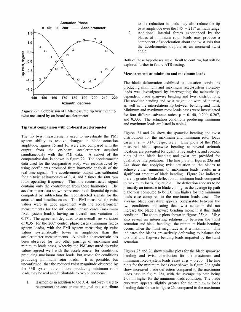
Tip twist comparison with on-board accelerometer The tip twist measurements used to investigate the PMI system ability to resolve changes in blade actuation amplitude, figures 15 and 16, were also compared with the output from the on-board accelerometer acquired simultaneously with the PMI data. A subset of the comparative data is shown in figure 22. The accelerometer data used for the comparative study was reconstructed by using coefficients produced from harmonic analysis of the real-time signal. The accelerometer output was calibrated for tip twist at harmonics of 3, 4, and 5 times the 688 rpm rotor operating frequency. Thus the reconstructed signal contains only the contribution from these harmonics. The accelerometer data shown represents the differential tip twist computed by subtracting the reconstructed signals for the actuated and baseline cases. The PMI-measured tip twist values were in good agreement with the accelerometer measurements for the 40° control phase cases (maximum fixed-system loads), having an overall rms variation of 0.17°. The agreement degraded to an overall rms variation of 0.35° for the 200° control phase cases (minimum fixed-system loads), with the PMI system measuring tip twist values systematically lower in amplitude than the accelerometer measurements. A similar characteristic has been observed for two other pairings of maximum and minimum loads cases, whereby the PMI-measured tip twist values agreed well with the accelerometer for conditions producing maximum rotor loads, but worse for conditions producing minimum rotor loads. It is possible, but unconfirmed, that the reduced twist magnitude observed by the PMI system at conditions producing minimum rotor loads may be real and attributable to two phenomena:

1. Harmonics in addition to the 3, 4, and 5/rev used to reconstruct the accelerometer signal that contribute

to the reduction in loads may also reduce the tip twist amplitude over the 145° − 215° azimuth range

2. Additional intertial forces experienced by the blades at minimum rotor loads may produce a component of acceleration about the twist axis that the accelerometer outputs as an increased twist angle.

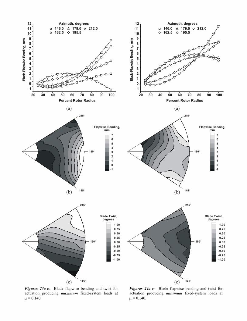
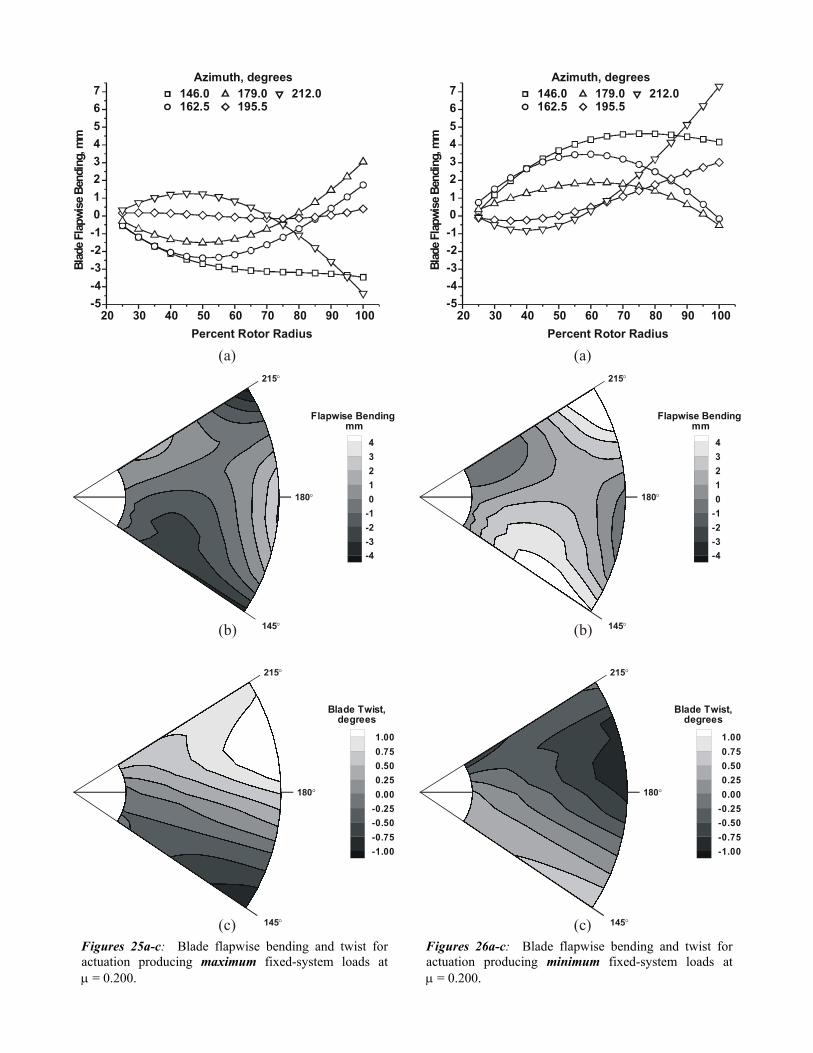
Both of these hypotheses are difficult to confirm, but will be explored further in future ATR testing. Measurements at minimum and maximum loads The blade deformation exhibited at actuation conditions producing minimum and maximum fixed-system vibratory loads was investigated by interrogating the azimuthally-dependent blade spanwise bending and twist distributions. The absolute bending and twist magnitude were of interest, as well as the interrelationship between bending and twist. Minimum and maximum rotor loads cases were investigated for four different advance ratios, µ = 0.140, 0.200, 0.267, and 0.333. The actuation conditions producing minimum and maximum loads are listed in table 4. Figures 23 and 24 show the spanwise bending and twist distributions for the maximum and minimum rotor loads cases at µ = 0.140 respectively. Line plots of the PMI-measured blade spanwise bending at several azimuth locations are presented for quantitative analysis, and contour plots of the blade bending and twist are provided for qualitative interpretation. The line plots in figures 23a and 24a show that applying twist actuation to the blades to achieve either minimum or maximum loads results in a significant amount of blade bending. Figure 24a indicates there is greater blade deflection at minimum loads compared to maximum loads, figure 23a. The deflection appears to be primarily an increase in blade coning, as the average tip path plane was computed to be 2.0 mm higher for the minimum loads case compared to the maximum loads case. The average blade curvature appears comparable between the two conditions, indicating that twist actuation did not increase the blade flapwise bending moment at this flight condition. The contour plots shown in figures 23b,c – 24b,c also reveal an interesting relationship between the twist actuation and blade bending: the minimum blade bending occurs when the twist magnitude is at a maximum. This indicates the blades are actively deforming to balance the torsional and flapwise bending loads imparted by the twist actuation. Figures 25 and 26 show similar plots for the blade spanwise bending and twist distribution for the maximum and minimum fixed-system loads cases at µ = 0.200. The line plots for the minimum loads case shown in figure 26a again show increased blade deflection compared to the maximum loads case in figure 25a, with the average tip path being 2.0 mm higher for the minimum loads condition. The blade curvature appears slightly greater for the minimum loads bending data shown in figure 26a compared to the maximum

140 150 160 170 180 190 200 210 220

-1.5

-1.0

-0.5

0.0

0.5

1.0

1.5

Tip

Twist

,deg

rees

Azimuth, degrees

40° 200° AccelerometerActuation Phase

Figure 22: Comparison of PMI-measured tip twist with tip twist measured by on-board accelerometer

(a)

(b)

(c)

(a)

(b)

(c)

Azimuth, degrees 146.0 162.5

179.0 195.5

212.0

20 30 40 50 60 70 80 90 100-10123456789

101112

Blad

eFl

apwi

seBe

ndin

g,m

m

Percent Rotor Radius

Azimuth, degrees 146.0 162.5

179.0 195.5

212.0

20 30 40 50 60 70 80 90 100-10123456789

101112

Blad

eFl

apwi

seBe

ndin

g,m

m

Percent Rotor Radius

76543210

-1

Flapwise Bendingmm

145°

180°

215°

,

76543210

-1

Flapwise Bendingmm

145°

180°

215°

,

1.000.750.500.250.00

-0.25-0.50-0.75-1.00

Blade Twist,degrees

145°

180°

215°

1.000.750.500.250.00

-0.25-0.50-0.75-1.00

Blade Twist,degrees

145°

180°

215°

Figures 23a-c: Blade flapwise bending and twist for actuation producing maximum fixed-system loads atµ = 0.140.

Figures 24a-c: Blade flapwise bending and twist for actuation producing minimum fixed-system loads atµ = 0.140.

20 30 40 50 60 70 80 90 100-5-4-3-2-101234567

Blad

eFlap

wise

Bend

ing,

mm

Percent Rotor Radius

Azimuth, degrees 146.0 162.5

179.0 195.5

212.0

43210

-1-2-3-4

Flapwise Bendingmm

145°

180°

215°

1.000.750.500.250.00

-0.25-0.50-0.75-1.00

Blade Twist,degrees

145°

180°

215°

20 30 40 50 60 70 80 90 100-5-4-3-2-101234567

Blad

eFlap

wise

Bend

ing,

mm

Percent Rotor Radius

Azimuth, degrees 146.0 162.5

179.0 195.5

212.0

43210

-1-2-3-4

Flapwise Bendingmm

145°

180°

215°

1.000.750.500.250.00

-0.25-0.50-0.75-1.00

Blade Twist,degrees

145°

180°

215°

(a)

(b)

(c)

(a)

(b)

(c)Figures 25a-c: Blade flapwise bending and twist for actuation producing maximum fixed-system loads atµ = 0.200.

Figures 26a-c: Blade flapwise bending and twist for actuation producing minimum fixed-system loads atµ = 0.200.

(a)

(b)

(c)

(a)

(b)

(c)

Azimuth, degrees 146.0 162.5

179.0 195.5

212.0Azimuth, degrees

146.0 162.5

179.0 195.5

212.0

20 30 40 50 60 70 80 90 100-6-5-4-3-2-10123456

Blad

eFl

apwi

seBe

ndin

g,m

m

Percent Rotor Radius20 30 40 50 60 70 80 90 100

-6-5-4-3-2-10123456

Blad

eFl

apwi

seBe

ndin

g,m

m

Percent Rotor Radius

1.000.750.500.250.00

-0.25-0.50-0.75-1.00

Blade Twist,degrees

145°

180°

215°

1.000.750.500.250.00

-0.25-0.50-0.75-1.00

Blade Twist,degrees

145°

180°

215°

21.510.50

-0.5-1-1.5-2

Flapwise Bendingmm

145°

180°

215°

,

21.510.50

-0.5-1-1.5-2

Flapwise Bendingmm

145°

180°

215°

,

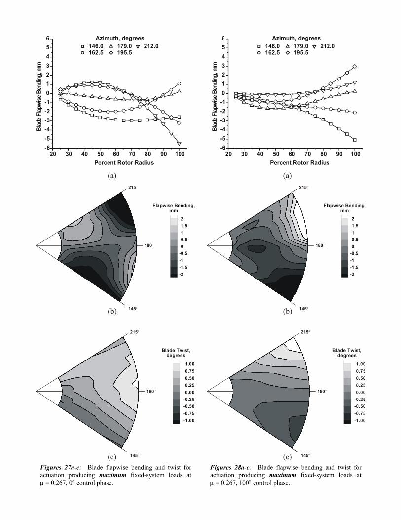
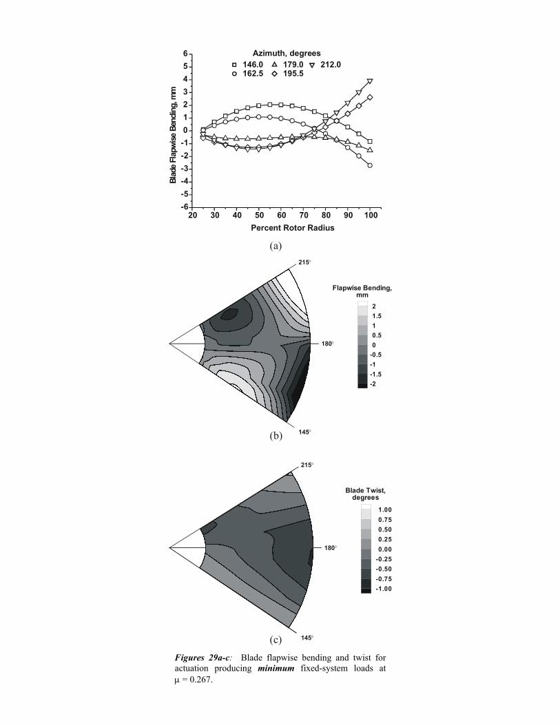
Figures 27a-c: Blade flapwise bending and twist for actuation producing maximum fixed-system loads atµ = 0.267, 0° control phase.

Figures 28a-c: Blade flapwise bending and twist for actuation producing maximum fixed-system loads atµ = 0.267, 100° control phase.

(a)

(b)

(c)

Azimuth, degrees 146.0 162.5

179.0 195.5

212.0

1.000.750.500.250.00

-0.25-0.50-0.75-1.00

Blade Twist,degrees

145°

180°

215°

20 30 40 50 60 70 80 90 100-6-5-4-3-2-10123456

Blad

eFl

apwi

seBe

ndin

g,m

m

Percent Rotor Radius

21.510.50

-0.5-1-1.5-2

Flapwise Bendingmm

145°

180°

215°

,

Figures 29a-c: Blade flapwise bending and twist for actuation producing minimum fixed-system loads atµ = 0.267.

(a)

(b)

(c)

(a)

(b)

(c)

Azimuth, degrees 146.0 162.5

179.0 195.5

212.0Azimuth, degrees

146.0 162.5

179.0 195.5

212.0

20 30 40 50 60 70 80 90 100-2.50.02.55.07.5

10.012.515.017.520.022.525.0

Blad

eFl

apwi

seBe

ndin

g,m

m

Percent Rotor Radius20 30 40 50 60 70 80 90 100

-2.50.02.55.07.5

10.012.515.017.520.022.525.0

Blad

eFl

apwi

seBe

ndin

g,m

m

Percent Rotor Radius

20.017.515.012.510.0

7.55.02.50.0

Flapwise Bendingmm

145°

180°

215°

,

20.017.515.012.510.0

7.55.02.50.0

Flapwise Bendingmm

145°

180°

215°

,

1.000.750.500.250.00

-0.25-0.50-0.75-1.00

Blade Twist,degrees

145°

180°

215°

1.000.750.500.250.00

-0.25-0.50-0.75-1.00

Blade Twist,degrees

145°

180°

215°

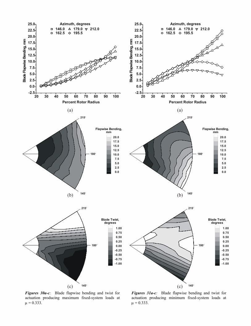
Figures 30a-c: Blade flapwise bending and twist for actuation producing maximum fixed-system loads atµ = 0.333.

Figures 31a-c: Blade flapwise bending and twist for actuation producing minimum fixed-system loads atµ = 0.333.

loads data shown in figure 25a, suggesting an increase in the blade flapwise bending moment at actuation conditions producing minimum loads. Examination of the contour plots in figures 25b,c and figures 26b,c again shows that minimum bending corresponds with maximum twist. PMI data were acquired at µ = 0.267 for two actuation cases that equivalently produced maximum fixed-system loads. These results are presented in figures 27 and 28 for 0° and 100° control phase respectively. The blade deformation results for the minimum loads case at µ = 0.267 is presented in figure 29. Note the actuation amplitude at µ = 0.267 was 750 volts versus 1000 volts for all other minimum/maximum loads cases studied. An overall reduction in blade bending and twist can be observed in the data accordingly. The data presented in figures 27 and 28 shows the blade spanwise bending and twist behavior was similar for the two maximum loads cases. In comparison with the minimum loads data shown in figure 29, no distinguishable difference can be seen in the height of the average blade tip path. However, the data shows a clear increase in blade bending for the minimum loads case of figure 29. This is particularly noticeable by examining the relatively high concentration of the contour lines in figure 29b compared to figures 27b and 28b. Therefore, as in the µ = 0.200 case, the bending data indicates an increase in flapwise bending moment at actuation conditions producing minimum fixed-system vibratory loads. The bending and twist contour plots shown in figures 27b, c – 29b, c again indicate that minimum blade bending coincides with maximum blade twist. The blade bending and twist data obtained for maximum and minimum loads cases at µ = 0.333 is shown in figures 30 and 31 respectively. The spanwise bending data shown in figures 30a and 31a show that actuating the blades at conditions producing either maximum or minimum loads increases the height of the blade tip path significantly. The blade bending data shown for the minimum loads case in figures 31a,b show a distinguishable increase in blade curvature compared to the maximum loads case of figures 30a,b. This again indicates an increase in blade flapwise bending moment for actuation conditions producing minimum loads. Although less noticeable because of the increase in steady state blade coning, figures 30b-c and 31b-c again indicate that minimum blade bending corresponds with maximum blade twist.

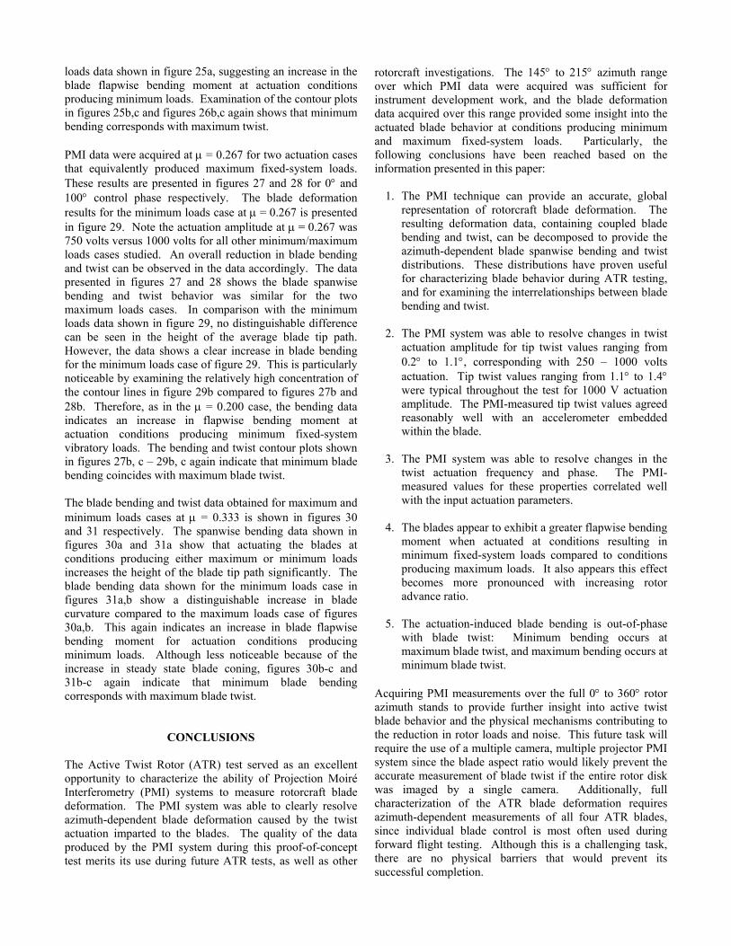
CONCLUSIONS The Active Twist Rotor (ATR) test served as an excellent opportunity to characterize the ability of Projection Moiré Interferometry (PMI) systems to measure rotorcraft blade deformation. The PMI system was able to clearly resolve azimuth-dependent blade deformation caused by the twist actuation imparted to the blades. The quality of the data produced by the PMI system during this proof-of-concept test merits its use during future ATR tests, as well as other

rotorcraft investigations. The 145° to 215° azimuth range over which PMI data were acquired was sufficient for instrument development work, and the blade deformation data acquired over this range provided some insight into the actuated blade behavior at conditions producing minimum and maximum fixed-system loads. Particularly, the following conclusions have been reached based on the information presented in this paper:

1. The PMI technique can provide an accurate, global representation of rotorcraft blade deformation. The resulting deformation data, containing coupled blade bending and twist, can be decomposed to provide the azimuth-dependent blade spanwise bending and twist distributions. These distributions have proven useful for characterizing blade behavior during ATR testing, and for examining the interrelationships between blade bending and twist.

2. The PMI system was able to resolve changes in twist

actuation amplitude for tip twist values ranging from 0.2° to 1.1°, corresponding with 250 – 1000 volts actuation. Tip twist values ranging from 1.1° to 1.4° were typical throughout the test for 1000 V actuation amplitude. The PMI-measured tip twist values agreed reasonably well with an accelerometer embedded within the blade.

3. The PMI system was able to resolve changes in the

twist actuation frequency and phase. The PMI-measured values for these properties correlated well with the input actuation parameters.

4. The blades appear to exhibit a greater flapwise bending

moment when actuated at conditions resulting in minimum fixed-system loads compared to conditions producing maximum loads. It also appears this effect becomes more pronounced with increasing rotor advance ratio.

5. The actuation-induced blade bending is out-of-phase

with blade twist: Minimum bending occurs at maximum blade twist, and maximum bending occurs at minimum blade twist.

Acquiring PMI measurements over the full 0° to 360° rotor azimuth stands to provide further insight into active twist blade behavior and the physical mechanisms contributing to the reduction in rotor loads and noise. This future task will require the use of a multiple camera, multiple projector PMI system since the blade aspect ratio would likely prevent the accurate measurement of blade twist if the entire rotor disk was imaged by a single camera. Additionally, full characterization of the ATR blade deformation requires azimuth-dependent measurements of all four ATR blades, since individual blade control is most often used during forward flight testing. Although this is a challenging task, there are no physical barriers that would prevent its successful completion.

ACKNOWLEGEMENTS The authors extend their appreciation to the U.S. Army Research Laboratory, Hampton, VA for providing wind tunnel time to conduct the PMI instrument development activities addressed in this paper.

REFERENCES 1. Lemnios, A. Z., and Howes, H. E., “Wind Tunnel

Investigation of the Controllable Twist Rotor Performance and Dynamic Behavior”, USAAMRDL-TR-77-10, Fort Eustis, VA., June, 1977.

2. Chen, P., and Chopra, I., “A Feasibility Study to Build a Smart Rotor: Induced Strain Actuation of Airfoil Twisting using Piezoceramic Crystals”, Proceedings of SPIE, Vol. 1917, Part 1, pp. 238-254, 1993.

3. Straub, F., “A Feasibility Study of Using Smart materials for Rotor Control”, Proceedings of the American Helicopter Society 49th Annual Forum, St. Louis, MO, May, 1993.

4. Derham, R. C., and Hagood, N. W., “Rotor Design Using Smart Materials to Actively Twist Blades”, Proceedings of the American Helicopter Society 52nd Annual Forum, Washington, DC, June 4 – 6, 1996.

5. Rodgers, J. P., Bent, A. A., and Hagood, N. W., “Characterization of interdigitated electrode piezoelectric fiber composites under high electrical and mechanical loading”, Proceedings of SPIE, Vol. 2717, pp. 642 – 659, 1996.

6. Patorski, K., Handbook of the Moiré Fringe Technique, Elsevier Science Publishers, 1993. pp. vii – xi, pp. 372-373.

7. Indebetouw, G., and Czarnek, R., editors, Selected Papers on Optical Moiré and Applications, SPIE Milestone Series, Vol. MS 64, 1992.

8. Fleming, G. A., Soto, H. L., South, B. W., and Bartram, S. M., “Advances in Projection Moiré Interferometry Development for Large Wind Tunnel Applications”, SAE Paper No. 1999-01-5598, SAE World Aviation Congress, San Francisco, CA, October 19-21, 1999.

9. Fleming, G. A., and Gorton, S. A., “Measurement of rotorcraft blade deformation using Projection Moiré Interferometry”, Journal of Shock and Vibration, Vol. 7, No. 3, 2000.

10. Fleming, G. A., and Burner, A. W., “Deformation measurements of smart aerodynamic surfaces”, Proceedings of SPIE, Vol. 3783, pp. 228 – 238, 1999.

11. Fleming, G. A., Bartram, S. M., Waszak, M. R., and Jenkins, L. N., “Projection Moiré Interferometry Measurements of Micro Air Vehicle Wings”, Proceedings of SPIE Vol. 4448, pp. 90 – 101, 2001.

12. Mercker, E., Pengel, K., Kube, R., Van der Wall, B., Boutier, A., Micheli, F., “On the Blade Deformation Measured at a Scaled Helicopter Rotor”, Proceedings on Aeromechanics Technology and Product Design, Bridgeport, CT, October 11-13, 1995.

13. Bruning, et al., “Digital wavefront measurement interferometer for testing optical surfaces and lenses”, Applied Optics, Vol. 30, pp. 2693-2703, 1974.

14. Ghiglia, D. C., and Pritt, M. D., Two-Dimensional Phase Unwrapping: Theory, Algorithms, and Software, John Wiley & Sons, Inc., New York, 1998.

15. Goldstein, R. M., Zebker, H. A., and Werner, C. L., “Satellite radar interferometry: two-dimensional phase unwrapping”, Radio Science, Vol. 23, (4), 1988, pp. 713 - 720.

16. Pirodda, L., “Shadow and projection moiré techniques for absolute or relative mapping of surface shapes”, Optical Engineering 21(4), pp. 640-649, July/August 1982.

17. J.F. Meyers, “Doppler Global Velocimetry - The Next Generation?”, paper AIAA-92-3897, Proceedings of the AIAA 17th Aerospace Ground Testing Conference, Nashville, TN, July 6-8 1992.

18. Phillips, D., “Image Processing in C, Part 14: Warping and Morphing”, C/C++ Users Journal, October, 1995, pp. 55 – 68.

19. Bass, M., editor, Handbook of Optics, Volume II – Devices, Measurements, and Properties, 2nd Edition. McGraw-Hill, Inc. New York, 1995, pp. 11.6.

20. Wilbur, M. L., Mirick, P. H., Yeager, W. T., Langston, C. W., Cesnik, C. E. S., and Shin, S-J., “Vibratory Loads Reduction Testing of the NASA/ARMY/MIT Active Twist Rotor”, Proceedings of the American Helicopter Society 57th Annual Forum, Washington, DC, May 9-11, 2001.

21. Wilbur, M. L., Yeager, W. T., Jr., and Sekula, M. K., "Further Examination of the Vibratory Loads Reduction Results from the NASA/Army/MIT Active Twist Rotor Test," Proceedings of the American Helicopter Society 58th Annual Forum, Montreal, Canada, June 11-13, 2002.

22. Booth Jr., E. R., and Wilbur, M. L., “Acoustic Aspects of Active Twist Rotor Control”, Proceedings of the American Helicopter Society 58th Annual Forum, Montréal, Canada, June 11-13, 2002.

23. “The NASA Langley Transonic Dynamics Tunnel”, NASA LWP-799, September, 1969.

24. Yeager, W. T., Jr., Mirick, P. H., Hamouda, M-N., Wilbur, M. L., Singleton, J. D., and Wilkie, W. K., "Rotorcraft Aeroelastic Testing in the Langley Transonic Dynamics Tunnel," Journal of the American Helicopter Society, Vol. 38, No. 3, July 1993, pp. 73-82.

25. Shin, S-J., Integral Twist Actuation of Helicopter Rotor Blades for Vibration Reduction, Ph. D. Dissertation, Massachusetts Institute of Technology, August, 2001.

26. Shin, S-J., and Cesnik, C. E. S., Design, manufacturing, and testing of an active twist rotor. AMSL #99-3, Massachusetts Institute of Technology, June, 1999.