Structural Dynamics Verification of Rotorcraft Comprehensive Analysis System (RCAS)

February 2005 • NREL/TP-500-35328

G.S. Bir

National Renewable Energy Laboratory 1617 Cole Boulevard, Golden, Colorado 80401-3393 303-275-3000 • www.nrel.gov

Operated for the U.S. Department of Energy Office of Energy Efficiency and Renewable Energy by Midwest Research Institute • Battelle

Contract No. DE-AC36-99-GO10337

National Renewable Energy Laboratory 1617 Cole Boulevard, Golden, Colorado 80401-3393 303-275-3000 • www.nrel.gov

Operated for the U.S. Department of Energy Office of Energy Efficiency and Renewable Energy by Midwest Research Institute • Battelle

Contract No. DE-AC36-99-GO10337

February 2005 • NREL/TP-500-35328

Structural Dynamics Verification of Rotorcraft Comprehensive Analysis System (RCAS)

G.S. Bir Prepared under Task No.WER5 3114

NOTICE

This report was prepared as an account of work sponsored by an agency of the United States government. Neither the United States government nor any agency thereof, nor any of their employees, makes any warranty, express or implied, or assumes any legal liability or responsibility for the accuracy, completeness, or usefulness of any information, apparatus, product, or process disclosed, or represents that its use would not infringe privately owned rights. Reference herein to any specific commercial product, process, or service by trade name, trademark, manufacturer, or otherwise does not necessarily constitute or imply its endorsement, recommendation, or favoring by the United States government or any agency thereof. The views and opinions of authors expressed herein do not necessarily state or reflect those of the United States government or any agency thereof.

Available electronically at http://www.osti.gov/bridge

Available for a processing fee to U.S. Department of Energy and its contractors, in paper, from:

U.S. Department of Energy Office of Scientific and Technical Information P.O. Box 62 Oak Ridge, TN 37831-0062 phone: 865.576.8401 fax: 865.576.5728 email: mailto:reports@adonis.osti.gov

Available for sale to the public, in paper, from: U.S. Department of Commerce National Technical Information Service 5285 Port Royal Road Springfield, VA 22161 phone: 800.553.6847 fax: 703.605.6900 email: orders@ntis.fedworld.gov online ordering: http://www.ntis.gov/ordering.htm

Printed on paper containing at least 50% wastepaper, including 20% postconsumer waste

iii

Executive Summary The Rotorcraft Comprehensive Analysis System (RCAS) was acquired and evaluated as part of an ongoing effort by the U.S Department of Energy (DOE) and the National Renewable Energy Laboratory (NREL) to provide state-of-the-art wind turbine modeling and analysis technology for Government and industry. RCAS is an interdisciplinary tool offering aeroelastic modeling and analysis options not supported by current codes. RCAS was developed during a 4-year joint effort among the U.S. Army’s Aeroflightdynamics Directorate, Advanced Rotorcraft Technology Inc., and the helicopter industry. The code draws heavily from its predecessor 2GCHAS (Second Generation Comprehensive Helicopter Analysis System), which required an additional 14 years to develop. Though developed for the rotorcraft industry, its general-purpose features allow it to model or analyze a general dynamic system. Its key feature is a specialized finite element that can model spinning flexible parts. The code, therefore, appears particularly suited for wind turbines whose dynamics is dominated by massive flexible spinning rotors. In addition to the simulation capability of the existing codes, RCAS [1-3] offers a range of unique capabilities, including aeroelastic stability analysis, trim, state-space modeling, operating modes, modal reduction, multi-blade coordinate transformation, periodic-system-specific analysis, choice of aerodynamic models, and a controls design/implementation graphical interface. These capabilities will likely become critical as wind turbines become larger and flexible, incorporating multivariable controls and novel design features (e.g., curved blades and stability augmentation mechanisms). RCAS also has a modular code structure, which allows it to readily absorb new technology as it becomes available (e.g., in the aerodynamics area).

A preliminary assessment in June 2002 showed that RCAS’s unique capabilities matched the demands of the wind industry, academia, and government agencies for advanced research, design, and analysis of existing—as well as evolving—wind turbine configurations, beyond the limitations imposed by the current codes. Management at the National Wind Technology Center (NWTC) recognized RCAS’s potential, but to thoroughly ensure that it was well suited for wind turbines, a more comprehensive evaluation of the code was mandated. It called for a three-part evaluation: a demonstration of RCAS’s ability to model wind turbines, aerodynamics verification, and dynamics verification. Jonkman et al. [4] demonstrated the ability of RCAS to model a three-bladed 1.5-MW wind turbine. Tangler et al. [5] performed the aerodynamics verification of RCAS.

This report focuses on the dynamics verification of RCAS. Verification implies checking workability of diverse modeling and analysis options in RCAS and assessing the accuracy of the results. We also attempt an assessment of RCAS’s user-friendliness and computational features. In addition, we provide a brief assessment of some unique features of RCAS that are not rigorously verifiable for lack of experimental data or another code with similar features.

The dynamics verification studies start with an elastic beam and progress to a full wind turbine model. Each model is built using RCAS and also ADAMS® (Automated Dynamic Analysis of Mechanical Systems) or UMARC (University of Maryland Advanced Rotorcraft Code) for comparative studies. If feasible, a corresponding analytical model is also developed. A variety of analyses are performed on each model, and the RCAS results are compared with those from ADAMS or UMARC. The analytical results, if available, are given the highest priority for verification. We pay special attention to the RCAS elastic beam modeling because a typical wind turbine’s dominant components are flexible and are frequently modeled as elastic beams (examples are tower, drivetrain shafts, and rotor blades; only the hub and the nacelle may be modeled as rigid bodies). When we progress to the full system model, all capabilities of RCAS are not directly verifiable. This is because ADAMS, the only general-purpose code available for side-by-side comparison, is limited to only two major capabilities: simulation and parked-turbine modal analysis. Jonkman et al. [4] verified these capabilities of RCAS. However, they made a few simplifications in the full-system RCAS model to permit comparison with ADAMS and FAST (Fatigue, Aerodynamics, Structures, and Turbulence) code. For our studies, we removed these simplifications by introducing a realistic gearbox, fully flexible low- and high-speed shafts, etc. Using the full system model,

iv

we exercised capabilities unique to RCAS (e.g., operating modes and stability analyses, multi-blade coordinate transformation, and modal reduction).

Verification studies confirm that RCAS is as accurate as ADAMS or UMARC. We were also able to exercise all the unique capabilities of RCAS without encountering any numerical instability or convergence problems. The results, although not directly verifiable, appeared physically viable and explainable. While performing simulation studies on the full system models, Jonkman [4] observed that RCAS computational time was an order of magnitude longer than that of ADAMS. In these studies, an identical number of degrees of freedom (DOFs) and time-step size were used for both the RCAS and ADAMS models. However, realizing that RCAS uses a more accurate finite element methodology compared to the lumped-properties approach ADAMS uses, we examined ways to reduce simulation time without sacrificing accuracy. We found that through a judicious choice of the number of finite elements, the modes for model reduction, and the number of Gaussian integration points within an element, the computational time may be reduced by a factor of 4 to 6 with only a 3%-5% accuracy loss.

Although RCAS allows accurate modeling and offers more capabilities than other codes, we found it as tedious to learn and use as ADAMS. The difficulty in usage is primarily due to the fact that output data from a typical RCAS run is difficult to extract in a user-friendly format. On the positive side, developing or modifying a dynamic model and running multiple analyses in RCAS are comparatively easy. Also, RCAS offers far more output options compared to ADAMS. Difficulty in learning is due to poorly written user’s manuals; these lack clear guidelines, definitions, and examples and also do not reflect the recent RCAS upgrades. An RCAS evaluation meeting was held recently at the NWTC and was attended by members from the wind industry, NREL, and Sandia. Although the code was deemed not ready for industry dissemination, there was a unanimous consensus to retain it as an in-house R&D code and use it for modeling and analyses not possible using current codes.

v

Table of Contents

1. Introduction......................................................................................................................... 1

2. Overview of RCAS Features .............................................................................................. 2

Structural Modeling Features............................................................................................ 2

Aerodynamic Modeling Features ...................................................................................... 5 Airload Models ................................................................................................................. 5 Induced Velocity Models.................................................................................................. 5

Controls Modeling Features............................................................................................... 6

Analysis Features ................................................................................................................ 6

3. Verification Approach........................................................................................................ 8

4. Verification Results............................................................................................................. 9

Tower .................................................................................................................................... 9 Uniform Beam Static Model............................................................................................. 9 Uniform Beam Dynamic Model ..................................................................................... 10 Non-Uniform Beam Model (non-rotating) ..................................................................... 11

Rotor Blades ...................................................................................................................... 12 Uniform Cable (Spinning) .............................................................................................. 12 Uniform Blade (Spinning) .............................................................................................. 13 Spinning Uniform Blade with Tip Mass......................................................................... 16 Non-Uniform Blade (Spinning) ...................................................................................... 16

Drivetrain........................................................................................................................... 19 Drivetrain Control Exercise ............................................................................................ 21

Full Wind Turbine System................................................................................................... 21 Operating Turbine Modes ............................................................................................... 23 Multi-Blade Coordinate Transformation ........................................................................ 23 Modal Reduction............................................................................................................. 24 System Response ............................................................................................................ 24

5. Critique of RCAS Capabilities and User-Friendliness.................................................. 26

6. Potential Usage of RCAS.................................................................................................. 29

Acknowledgments ................................................................................................................. 29

References.............................................................................................................................. 30

APPENDIX A: RCAS Scripts................................................................................................ 1

A1. RCAS Script for the Rotating Blade .......................................................................... 1 Non-Uniform Blade Properties Data File ......................................................................... 6 Uniform Blade Properties Data File ............................................................................... 10 Uniform Cable Properties Data File ............................................................................... 11

vi

A2. RCAS Script for the Drivetrain.................................................................................. 1 Low-Speed Shaft Properties Data File.............................................................................. 6

A3. RCAS Script for the Drivetrain Control.................................................................... 1 Controls Interface File (komgsq.cmd) ............................................................................ 11

A4. RCAS Script for the Full Turbine System................................................................. 1 Tower Properties Data File ............................................................................................. 12

1

1. Introduction Over the past few years, FAST and ADAMS® have been successfully used by the U.S. wind industry, the National Renewable Energy Laboratory (NREL), and the National Wind Technology Center (NWTC) for predicting the dynamic response, loads, and fatigue life of wind turbines. FAST (Fatigue, Aerodynamics, Structures, and Turbulence) [6] is a wind-turbine-specific structural dynamic code originally developed by Oregon State University and the University of Utah and later extensively upgraded by NWTC researchers [7]. ADAMS [8-9], or Automated Dynamic Analysis of Mechanical Systems, is a commercial, general-purpose, dynamics code available from the MSC.Software Corporation that is capable of modeling wind turbines using a multi-rigid-body approach. Both FAST and ADAMS are usually coupled with the University of Utah’s AeroDyn aerodynamics package [10] to allow aeroelastic simulations.

Unfortunately, these codes do not offer some key capabilities required for a more comprehensive analysis and design of large, flexible wind turbines using multivariable controls or unconventional design features. Examples of capabilities not supported by the existing codes include finite element methodology, aeroelastic stability analysis, trim, state-space modeling, operating modes, modal reduction, multi-blade coordinate transformation, periodic-system-specific analyses, multiple aerodynamic modeling options, and a controls design interface. The Rotorcraft Comprehensive Analysis System (RCAS) [1-3], the most advanced aeroelastic code currently available, has the potential to fill this void. The code was jointly developed by the U.S. Army’s Aeroflightdynamics Directorate, the Advanced Rotorcraft Technology (ART), and the helicopter industry over a 4-year period. The code heavily draws from its predecessor 2GCHAS (Second Generation Comprehensive Helicopter Analysis System), which took an additional 14 years to develop. Though developed for the rotorcraft industry, its general-purpose features allow it to model or analyze a general-configuration aeroelastic system, including wind turbines. Also, the code is free to U.S. industries and government agencies.

The key feature of RCAS is a specialized finite element that accurately captures the large-deflection, centrifugal, and gyroscopic effects associated with spinning flexible rotors. The code, therefore, appears particularly suited for wind turbines whose dynamics are dominated by a massive rotor that behaves like a flexible gyroscope coupled to a tall flexible tower via a flexible drivetrain. The code has the flexibility to model conventional configurations (including teeter, deta-3, and an arbitrary number of twisted, tapered blades), as well as unconventional configurations (including offshore turbine designs, variable-swept blades, multi-axis gearboxes, complex hub and blade-pitch mechanisms). It incorporates a broad range of aerodynamic modules, including those available in the AeroDyn, and advanced control modules available in a Simulink®-like graphical environment.

Motivated by RCAS’s extensive range of modeling and analysis capabilities, its ability to absorb new research (especially in the aerodynamics area), and its long development history, we decided to evaluate its applicability to wind turbines. The evaluation study was divided into three parts: a demonstration of RCAS’s ability to model wind turbines, dynamics verification, and aerodynamics verification. Report [4] demonstrates the ability of RCAS to model a three-bladed, 1.5-MW wind turbine using a side-by-side comparison of RCAS-predicted responses with those predicted by ADAMS and FAST. In this report, the tower and the blades were modeled as fully flexible beams, but the drivetrain model was simplified to permit comparison with ADAMS and FAST (e.g., the gearbox was eliminated and the high-speed and low-speed shaft were assumed rigid joined by a single torsion spring). Report [5] covers the aerodynamics verification of RCAS; a rigid-blade rotor was used to eliminate aeroelastic feedback effects and concentrate on aerodynamics only.

This report focuses on the structural dynamics verification of RCAS. The report also provides an evaluation of some unique features of RCAS that are not rigorously verifiable for lack of experimental data or another code with similar features. Finally, the report attempts an assessment of RCAS’s user-friendliness and computational features.

2

The next section provides an overview of RCAS, including a brief description of its structural and aerodynamic features. Section 2 describes the dynamics verification approach and Section 4 provides detailed verification results. Particular attention is paid to the elastic beam because it uses novel finite elements and represents all the major and flexible components of a wind turbine (the tower, the blades, and the drivetrain). Section 5 critiques RCAS’s capabilities, user-friendliness, and computational features. The report concludes with Section 6 and a discussion of potential applications for RCAS.

2. Overview of RCAS Features RCAS is a comprehensive, multi-disciplinary computer code capable of modeling complex, general configurations and analyzing them under a broad range of operating conditions. Though primarily intended for rotorcraft research and engineering design, its general-purpose capabilities make it suitable for wind turbines as well. It is a significantly improved version of the original comprehensive computer code known as the Second Generation Comprehensive Helicopter Analysis System (2GCHAS). While retaining all functionalities of 2GCHAS, RCAS offers improved numerical schemes for computational efficiency, ability to handle large motions, a substantially improved nonlinear beam element, and an interactive user interface. The RCAS documentation is derived from the 2GCHAS manuals, which were originally developed by several organizations: Advanced Rotorcraft Technology, Inc.; Boeing Helicopters; Computer Science Corporation; Johnson Aeronautics; Kaman Aerospace Corporation; McDonnell Douglas Helicopter Company; Sterling Software; Federal Systems Group; United Technologies; and Sikorsky Aircraft. RCAS is available from the Aero Flightdynamics Directorate as a nonproprietary rotorcraft simulation system for use by the government and government-approved agencies. Below we summarize RCAS’s salient features and its modeling approach.

Structural Modeling Features RCAS is the only code available that simultaneously offers finite-element-based multi-flexible-body modeling, state-space linearization, and applicability to rotating structures. NASTRAN is also a multi-body finite element code, but its elements fail to adequately capture the gyroscopic and centrifugal stiffening effects associated with a rotating structure. RCAS uses a special nonlinear beam finite element that overcomes these deficiencies. ADAMS is a multi-rigid-body code, but a judicious combination of rigid and discreet spring elements allows ADAMS to model a general flexible structure quite adequately. For almost a decade, ADAMS has been successfully used to model and analyze a variety of wind turbines. A user typically employs a large number of elements to compensate for the loss of accuracy offered by a multi-flexible-body. However, ADAMS lacks capabilities like state-space modeling for controls, aeroelastic stability analysis, etc.

Like other multi-body codes, RCAS offers a variety of structural elements that may be connected arbitrarily to model a complex general system. RCAS has a far more extensive library of structural elements than ADAMS, which uses only rigid-body, force, and field (spring-damper) elements. RCAS does not have a library of constraints, though. The elements implicitly take care of the constraints; this has pros and cons. The advantages are that the number of equations required for modeling is greatly reduced and that no differential-algebraic equations are required with their attendant numerical instability problems. The disadvantage is that one must rely on a recursive formulation and solution of system equations to account for the inter-element forces and displacements; RCAS uses a force-residual recursive scheme. Among the structural elements RCAS uses, the nonlinear beam and the gearbox elements deserve attention.

The RCAS beam element has a few unique features. Its underlying formulation includes the pertinent nonlinear geometric terms associated with gyroscopic and centrifugal effects. Also, a finite element assembly based on deformed coordinates allows for very large beam deflections; even a wrap-around of a

3

flexible beam is admissible. The beam element has a maximum of 15 degrees of freedom, or DOFs (4 for flap, 4 for lag, 3 for torsion, and 4 for axial displacements) and a maximum of 5 nodes (two external and three internal). A user may opt to retain only the flap DOF, only the lag DOF, only the torsion DOF, only the axial DOF, or any combination of these. This is a unique and useful capability that ADAMS does not offer. Also, different number of Gaussian integration points may be specified for the beam elements. This variable specification of Gaussian points is a useful feature. For example, a user may wish to specify more Gaussian points, and hence a more accurate integration, over elements with rapid variation of structural or aerodynamic properties, and fewer Gaussian points for elements with relatively smooth variation of properties. Computational time versus desired accuracy thus may be balanced. The beam element formulation accepts arbitrary variation of section mass, inertia, flap and edgewise stiffness, torsion and axial stiffness, elastic-axis offset, center-of-mass offset, and tension-center offset. As for composite modeling capability, the element does have provisions for admitting cross-coupled stiffness properties. But RCAS does not yet provide any preprocessor to derive these cross-coupled terms from user-specified composite material structural and geometric properties.

The gearbox element allows specification of multiple input or output shafts oriented arbitrarily in the three-dimensional space. It also allows specification of inertia properties and damping for its gears. Thus, the gearbox is truly a dynamic element, unlike the pure kinematic, single-axis element used in ADAMS. It also does not appear to cause any numerical convergence problems, as does the ADAMS element for high gear ratios.

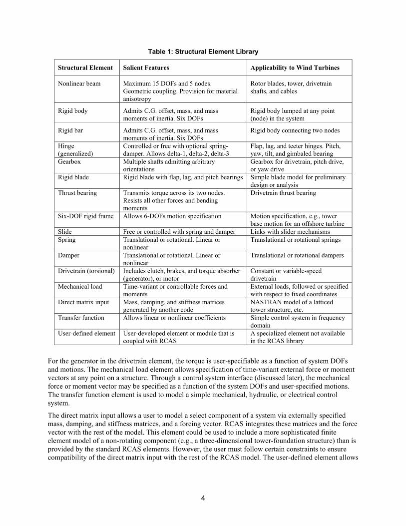
Each element listed in Table 1 is distinguishable by its type, its nodes available for connection to the rest of the system, and its properties. An element has at least one node. Most have two: a parent node and a child node. Some elements, such as springs and dampers, have more than one parent node, and some elements, like the nonlinear beam element, have multiple children nodes (aerodynamic nodes and end nodes). During assembly, the root node of each element attaches rigidly to the end node of its parent element. This means the motion of the child node of an element defines the motion of the parent node of its child element. Structural constraints are implemented by including elements such as hinges and slides. A detailed descriptions and mathematical basis of these elements is presented in Chapter 4 of the RCAS Theory Manual [1]. The nonlinear beam will undoubtedly be the most widely used element for wind turbines because of its ability to model rotor blades, tower, and the drivetrain shafts.

The rigid body element has only one node and is used for lumping mass or inertia at a single point on a structure. We may use it, for example, to model a concentrated inertia at the tip node of a blade. The rigid bar element, on the other hand, has two nodes and is used to model very stiff structures joining two points on a structure. Its typical use would be modeling nacelle and hub components. The rigid blade element provides a simpler model of the rotor blade than would be obtained through nonlinear beam elements. It represents a rigid structure with three hinges: flap hinge, lag hinge, and pitch bearing. The hinges may be preset at arbitrary angles and placed in any sequence at desired radial locations; the radial locations may or may not be coincident. Rotational springs and dampers may be included for any of the hinges. All three rigid elements described in this paragraph allow center-of-mass offset with respect to their nodal points of attachment. The spring and the damper are both two-node elements, which allow translational or rotational displacement at their end nodes. These elements can model linear or nonlinear spring-dampers.

4

Table 1: Structural Element Library

Structural Element Salient Features Applicability to Wind Turbines

Nonlinear beam Maximum 15 DOFs and 5 nodes. Geometric coupling. Provision for material anisotropy

Rotor blades, tower, drivetrain shafts, and cables

Rigid body Admits C.G. offset, mass, and mass moments of inertia. Six DOFs

Rigid body lumped at any point (node) in the system

Rigid bar Admits C.G. offset, mass, and mass moments of inertia. Six DOFs

Rigid body connecting two nodes

Hinge (generalized)

Controlled or free with optional spring-damper. Allows delta-1, delta-2, delta-3

Flap, lag, and teeter hinges. Pitch, yaw, tilt, and gimbaled bearing

Gearbox Multiple shafts admitting arbitrary orientations

Gearbox for drivetrain, pitch drive, or yaw drive

Rigid blade Rigid blade with flap, lag, and pitch bearings Simple blade model for preliminary design or analysis

Thrust bearing Transmits torque across its two nodes. Resists all other forces and bending moments

Drivetrain thrust bearing

Six-DOF rigid frame Allows 6-DOFs motion specification Motion specification, e.g., tower base motion for an offshore turbine

Slide Free or controlled with spring and damper Links with slider mechanisms Spring Translational or rotational. Linear or

nonlinear Translational or rotational springs

Damper Translational or rotational. Linear or nonlinear

Translational or rotational dampers

Drivetrain (torsional) Includes clutch, brakes, and torque absorber (generator), or motor

Constant or variable-speed drivetrain

Mechanical load Time-variant or controllable forces and moments

External loads, followed or specified with respect to fixed coordinates

Direct matrix input Mass, damping, and stiffness matrices generated by another code

NASTRAN model of a latticed tower structure, etc.

Transfer function Allows linear or nonlinear coefficients Simple control system in frequency domain

User-defined element User-developed element or module that is coupled with RCAS

A specialized element not available in the RCAS library

For the generator in the drivetrain element, the torque is user-specifiable as a function of system DOFs and motions. The mechanical load element allows specification of time-variant external force or moment vectors at any point on a structure. Through a control system interface (discussed later), the mechanical force or moment vector may be specified as a function of the system DOFs and user-specified motions. The transfer function element is used to model a simple mechanical, hydraulic, or electrical control system.

The direct matrix input allows a user to model a select component of a system via externally specified mass, damping, and stiffness matrices, and a forcing vector. RCAS integrates these matrices and the force vector with the rest of the model. This element could be used to include a more sophisticated finite element model of a non-rotating component (e.g., a three-dimensional tower-foundation structure) than is provided by the standard RCAS elements. However, the user must follow certain constraints to ensure compatibility of the direct matrix input with the rest of the RCAS model. The user-defined element allows

5

a user to supply an external subroutine that calculates matrices for an element not available in the RCAS standard library.

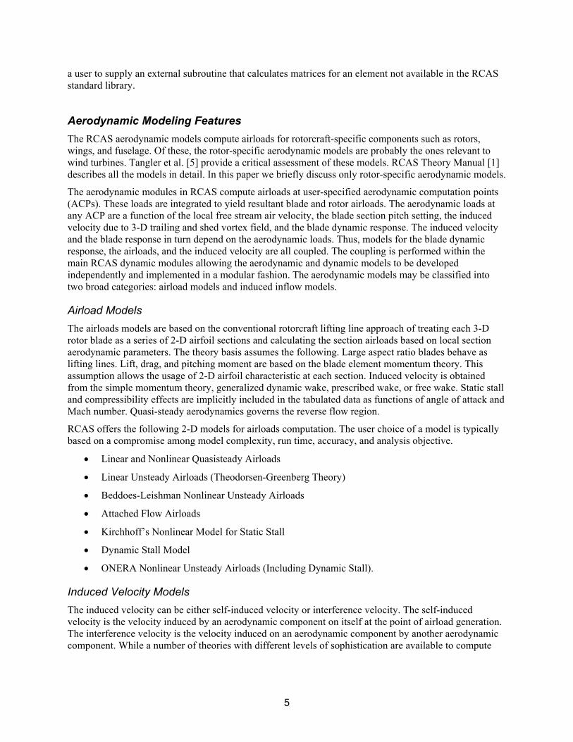
Aerodynamic Modeling Features The RCAS aerodynamic models compute airloads for rotorcraft-specific components such as rotors, wings, and fuselage. Of these, the rotor-specific aerodynamic models are probably the ones relevant to wind turbines. Tangler et al. [5] provide a critical assessment of these models. RCAS Theory Manual [1] describes all the models in detail. In this paper we briefly discuss only rotor-specific aerodynamic models.

The aerodynamic modules in RCAS compute airloads at user-specified aerodynamic computation points (ACPs). These loads are integrated to yield resultant blade and rotor airloads. The aerodynamic loads at any ACP are a function of the local free stream air velocity, the blade section pitch setting, the induced velocity due to 3-D trailing and shed vortex field, and the blade dynamic response. The induced velocity and the blade response in turn depend on the aerodynamic loads. Thus, models for the blade dynamic response, the airloads, and the induced velocity are all coupled. The coupling is performed within the main RCAS dynamic modules allowing the aerodynamic and dynamic models to be developed independently and implemented in a modular fashion. The aerodynamic models may be classified into two broad categories: airload models and induced inflow models.

Airload Models The airloads models are based on the conventional rotorcraft lifting line approach of treating each 3-D rotor blade as a series of 2-D airfoil sections and calculating the section airloads based on local section aerodynamic parameters. The theory basis assumes the following. Large aspect ratio blades behave as lifting lines. Lift, drag, and pitching moment are based on the blade element momentum theory. This assumption allows the usage of 2-D airfoil characteristic at each section. Induced velocity is obtained from the simple momentum theory, generalized dynamic wake, prescribed wake, or free wake. Static stall and compressibility effects are implicitly included in the tabulated data as functions of angle of attack and Mach number. Quasi-steady aerodynamics governs the reverse flow region.

RCAS offers the following 2-D models for airloads computation. The user choice of a model is typically based on a compromise among model complexity, run time, accuracy, and analysis objective.

• Linear and Nonlinear Quasisteady Airloads

• Linear Unsteady Airloads (Theodorsen-Greenberg Theory)

• Beddoes-Leishman Nonlinear Unsteady Airloads

• Attached Flow Airloads

• Kirchhoff’s Nonlinear Model for Static Stall

• Dynamic Stall Model

• ONERA Nonlinear Unsteady Airloads (Including Dynamic Stall).

Induced Velocity Models The induced velocity can be either self-induced velocity or interference velocity. The self-induced velocity is the velocity induced by an aerodynamic component on itself at the point of airload generation. The interference velocity is the velocity induced on an aerodynamic component by another aerodynamic component. While a number of theories with different levels of sophistication are available to compute

6

induced velocity distributions, only the most frequently used for rotorcraft analyses are considered in RCAS. For the rotor, RCAS offers the following

• Uniform inflow based momentum theory

• Generalized dynamic wake (Peter and He)

• Prescribed wake

• Free wake.

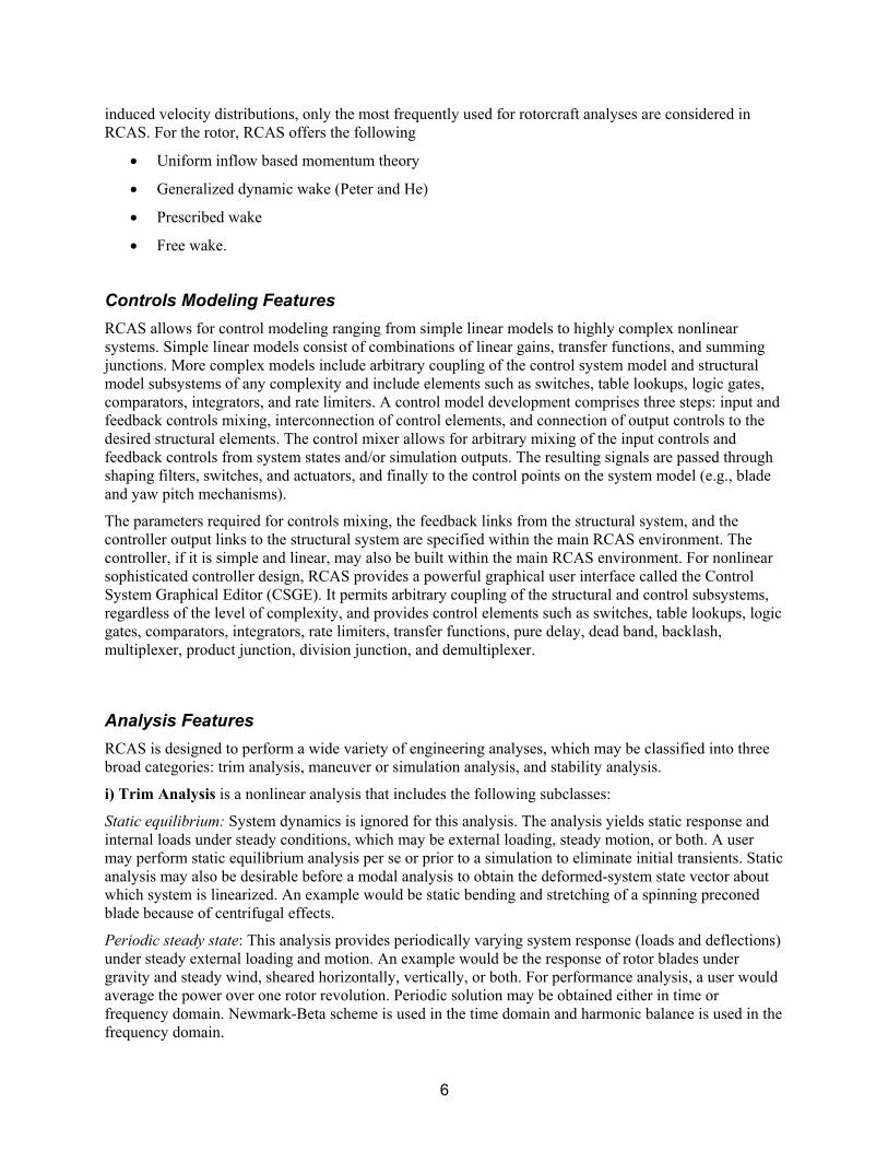
Controls Modeling Features RCAS allows for control modeling ranging from simple linear models to highly complex nonlinear systems. Simple linear models consist of combinations of linear gains, transfer functions, and summing junctions. More complex models include arbitrary coupling of the control system model and structural model subsystems of any complexity and include elements such as switches, table lookups, logic gates, comparators, integrators, and rate limiters. A control model development comprises three steps: input and feedback controls mixing, interconnection of control elements, and connection of output controls to the desired structural elements. The control mixer allows for arbitrary mixing of the input controls and feedback controls from system states and/or simulation outputs. The resulting signals are passed through shaping filters, switches, and actuators, and finally to the control points on the system model (e.g., blade and yaw pitch mechanisms).

The parameters required for controls mixing, the feedback links from the structural system, and the controller output links to the structural system are specified within the main RCAS environment. The controller, if it is simple and linear, may also be built within the main RCAS environment. For nonlinear sophisticated controller design, RCAS provides a powerful graphical user interface called the Control System Graphical Editor (CSGE). It permits arbitrary coupling of the structural and control subsystems, regardless of the level of complexity, and provides control elements such as switches, table lookups, logic gates, comparators, integrators, rate limiters, transfer functions, pure delay, dead band, backlash, multiplexer, product junction, division junction, and demultiplexer.

Analysis Features RCAS is designed to perform a wide variety of engineering analyses, which may be classified into three broad categories: trim analysis, maneuver or simulation analysis, and stability analysis.

i) Trim Analysis is a nonlinear analysis that includes the following subclasses:

Static equilibrium: System dynamics is ignored for this analysis. The analysis yields static response and internal loads under steady conditions, which may be external loading, steady motion, or both. A user may perform static equilibrium analysis per se or prior to a simulation to eliminate initial transients. Static analysis may also be desirable before a modal analysis to obtain the deformed-system state vector about which system is linearized. An example would be static bending and stretching of a spinning preconed blade because of centrifugal effects.

Periodic steady state: This analysis provides periodically varying system response (loads and deflections) under steady external loading and motion. An example would be the response of rotor blades under gravity and steady wind, sheared horizontally, vertically, or both. For performance analysis, a user would average the power over one rotor revolution. Periodic solution may be obtained either in time or frequency domain. Newmark-Beta scheme is used in the time domain and harmonic balance is used in the frequency domain.

7

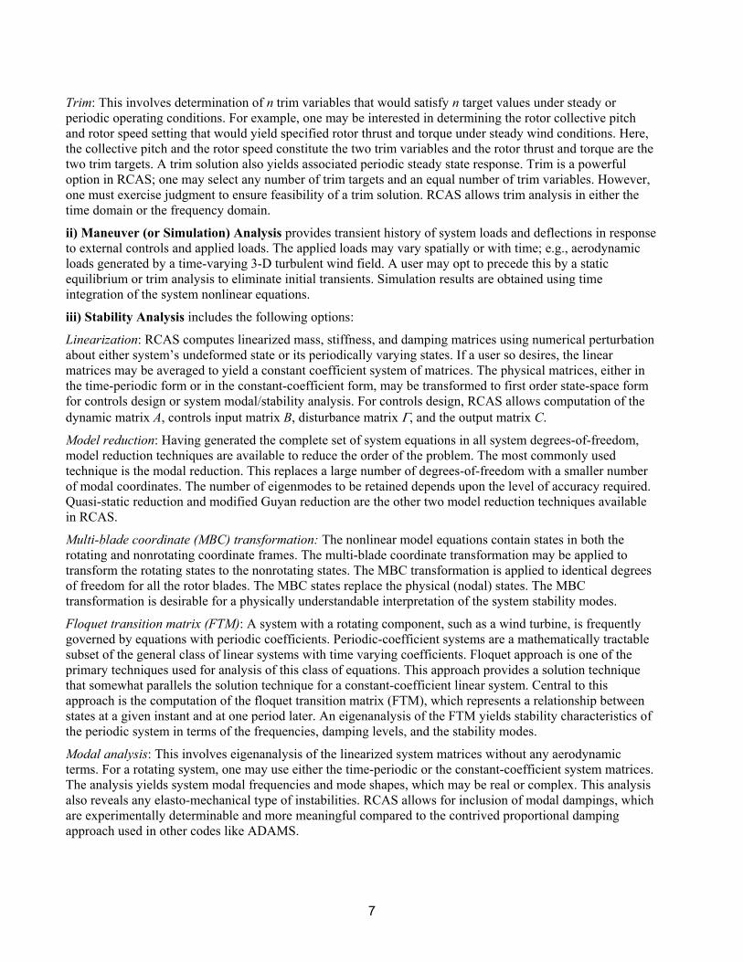
Trim: This involves determination of n trim variables that would satisfy n target values under steady or periodic operating conditions. For example, one may be interested in determining the rotor collective pitch and rotor speed setting that would yield specified rotor thrust and torque under steady wind conditions. Here, the collective pitch and the rotor speed constitute the two trim variables and the rotor thrust and torque are the two trim targets. A trim solution also yields associated periodic steady state response. Trim is a powerful option in RCAS; one may select any number of trim targets and an equal number of trim variables. However, one must exercise judgment to ensure feasibility of a trim solution. RCAS allows trim analysis in either the time domain or the frequency domain.

ii) Maneuver (or Simulation) Analysis provides transient history of system loads and deflections in response to external controls and applied loads. The applied loads may vary spatially or with time; e.g., aerodynamic loads generated by a time-varying 3-D turbulent wind field. A user may opt to precede this by a static equilibrium or trim analysis to eliminate initial transients. Simulation results are obtained using time integration of the system nonlinear equations.

iii) Stability Analysis includes the following options:

Linearization: RCAS computes linearized mass, stiffness, and damping matrices using numerical perturbation about either system’s undeformed state or its periodically varying states. If a user so desires, the linear matrices may be averaged to yield a constant coefficient system of matrices. The physical matrices, either in the time-periodic form or in the constant-coefficient form, may be transformed to first order state-space form for controls design or system modal/stability analysis. For controls design, RCAS allows computation of the dynamic matrix A, controls input matrix B, disturbance matrix Γ, and the output matrix C.

Model reduction: Having generated the complete set of system equations in all system degrees-of-freedom, model reduction techniques are available to reduce the order of the problem. The most commonly used technique is the modal reduction. This replaces a large number of degrees-of-freedom with a smaller number of modal coordinates. The number of eigenmodes to be retained depends upon the level of accuracy required. Quasi-static reduction and modified Guyan reduction are the other two model reduction techniques available in RCAS.

Multi-blade coordinate (MBC) transformation: The nonlinear model equations contain states in both the rotating and nonrotating coordinate frames. The multi-blade coordinate transformation may be applied to transform the rotating states to the nonrotating states. The MBC transformation is applied to identical degrees of freedom for all the rotor blades. The MBC states replace the physical (nodal) states. The MBC transformation is desirable for a physically understandable interpretation of the system stability modes.

Floquet transition matrix (FTM): A system with a rotating component, such as a wind turbine, is frequently governed by equations with periodic coefficients. Periodic-coefficient systems are a mathematically tractable subset of the general class of linear systems with time varying coefficients. Floquet approach is one of the primary techniques used for analysis of this class of equations. This approach provides a solution technique that somewhat parallels the solution technique for a constant-coefficient linear system. Central to this approach is the computation of the floquet transition matrix (FTM), which represents a relationship between states at a given instant and at one period later. An eigenanalysis of the FTM yields stability characteristics of the periodic system in terms of the frequencies, damping levels, and the stability modes.

Modal analysis: This involves eigenanalysis of the linearized system matrices without any aerodynamic terms. For a rotating system, one may use either the time-periodic or the constant-coefficient system matrices. The analysis yields system modal frequencies and mode shapes, which may be real or complex. This analysis also reveals any elasto-mechanical type of instabilities. RCAS allows for inclusion of modal dampings, which are experimentally determinable and more meaningful compared to the contrived proportional damping approach used in other codes like ADAMS.

8

Aeroelastic stability analysis: This involves eigenanalysis of the linearized system matrices with aerodynamic terms included. Again, one may use either the time-periodic or the constant-coefficient system matrices. The analysis yields stability mode shapes, associated frequencies, and damping levels. A typical stability analysis involves two steps: linearization and linear analysis. Linearization is usually preceded by a trim analysis and followed by model reduction and the MBC transformation mentioned above.

The trim analysis, the maneuver analysis, and computation of the floquet transition matrix require time integration, which is performed using the extended Newmark-Beta method. This method is unconditionally stable for linear systems. It is second-order accurate, easy to use, and depends only on system states from the previous time step. Nonlinearities may render the Newmark-Beta method unstable. This is more likely for high-frequency modes for which the integration time step may become too large. For most dynamic response cases, the participation of higher modes is small and may be ignorable. For cases in which higher modes become important, the time integration step must be reduced. RCAS uses the Hilber-Hughes-Taylor (HHT) extension of the Newmark-Beta method, which provides numerical damping for the higher modes, yet has little effect on the low-frequency modes. 3. Verification Approach As mentioned earlier, this report focuses on the structural dynamic of RCAS; aerodynamic verification is covered in a separate report [5]. We performed the verification in two phases. First, we critically examined the RCAS theory basis (i.e., formulation of structural elements, assembly procedure, time integration approach, and schemes underlying RCAS-specific analyses). Though no technical errors were found, it took inordinate time and effort to follow the theoretical developments because of the following reasons: poor technical writing, vague definitions, incomplete description of several concepts, and lack of explanatory figures and examples. The Advanced Rotorcraft Technology had to be consulted frequently to seek clarifications. Two technical details concerned us. One was the lack of description for the multi-axis and multi-node gearbox element. The other was the thrust-bearing element, which though described well, assumed that the drivetrain axial constraint and its constant speed, if required, occurred at the same location. This assumption, though not an overriding technical concern (ADAMS modeling tacitly makes the same assumption), was inconsistent with the degree of modeling flexibility we expected from RCAS. If one is interested in load paths experienced by a detailed drivetrain model, this assumption may lead to erroneous results. Both of these concerns have been conveyed to Advanced Rotorcraft Technology (ART) members, and they are resolving these.

In the second phase, we performed verification studies on the RCAS code. To this end, we developed several structural models using RCAS. Similar models were developed for side-by-side comparisons with RCAS using one of the following:

• Analytical formulation

• UMARC code

• ADAMS code.

The analytical formulation was given the highest priority because it provided exact results. However, analytical results were obtainable for a few simple cases only. We accorded the next priority to models developed using the University of Maryland Rotorcraft Code, UMARC [11]. Like RCAS, this code is also finite-element-based and has been extensively validated with both analytical and experimental data. However, UMARC is rotorcraft-specific, and we could use it only to validate RCAS’s capability to model flexible tower and rotor blades. Because it lacks general-configuration modeling capability, we could not use it for validating the full wind turbine system. We used ADAMS instead.

9

Table 2: Models Used for Structural Dynamic Verification

RCAS Model Set to be Verified

Code Used for Side-By-Side Comparison

Tower models Analytical and UMARC

Rotor blades (uniform) Analytical and UMARC

Rotor blades (non-uniform) UMARC

Drivetrain Analytical

Full wind turbine model ADAMS

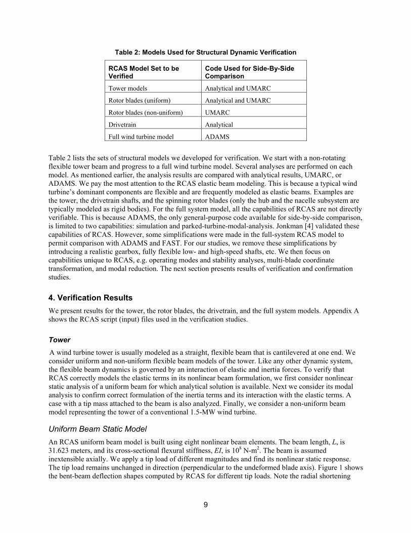
Table 2 lists the sets of structural models we developed for verification. We start with a non-rotating flexible tower beam and progress to a full wind turbine model. Several analyses are performed on each model. As mentioned earlier, the analysis results are compared with analytical results, UMARC, or ADAMS. We pay the most attention to the RCAS elastic beam modeling. This is because a typical wind turbine’s dominant components are flexible and are frequently modeled as elastic beams. Examples are the tower, the drivetrain shafts, and the spinning rotor blades (only the hub and the nacelle subsystem are typically modeled as rigid bodies). For the full system model, all the capabilities of RCAS are not directly verifiable. This is because ADAMS, the only general-purpose code available for side-by-side comparison, is limited to two capabilities: simulation and parked-turbine-modal-analysis. Jonkman [4] validated these capabilities of RCAS. However, some simplifications were made in the full-system RCAS model to permit comparison with ADAMS and FAST. For our studies, we remove these simplifications by introducing a realistic gearbox, fully flexible low- and high-speed shafts, etc. We then focus on capabilities unique to RCAS, e.g. operating modes and stability analyses, multi-blade coordinate transformation, and modal reduction. The next section presents results of verification and confirmation studies. 4. Verification Results We present results for the tower, the rotor blades, the drivetrain, and the full system models. Appendix A shows the RCAS script (input) files used in the verification studies.

Tower A wind turbine tower is usually modeled as a straight, flexible beam that is cantilevered at one end. We consider uniform and non-uniform flexible beam models of the tower. Like any other dynamic system, the flexible beam dynamics is governed by an interaction of elastic and inertia forces. To verify that RCAS correctly models the elastic terms in its nonlinear beam formulation, we first consider nonlinear static analysis of a uniform beam for which analytical solution is available. Next we consider its modal analysis to confirm correct formulation of the inertia terms and its interaction with the elastic terms. A case with a tip mass attached to the beam is also analyzed. Finally, we consider a non-uniform beam model representing the tower of a conventional 1.5-MW wind turbine.

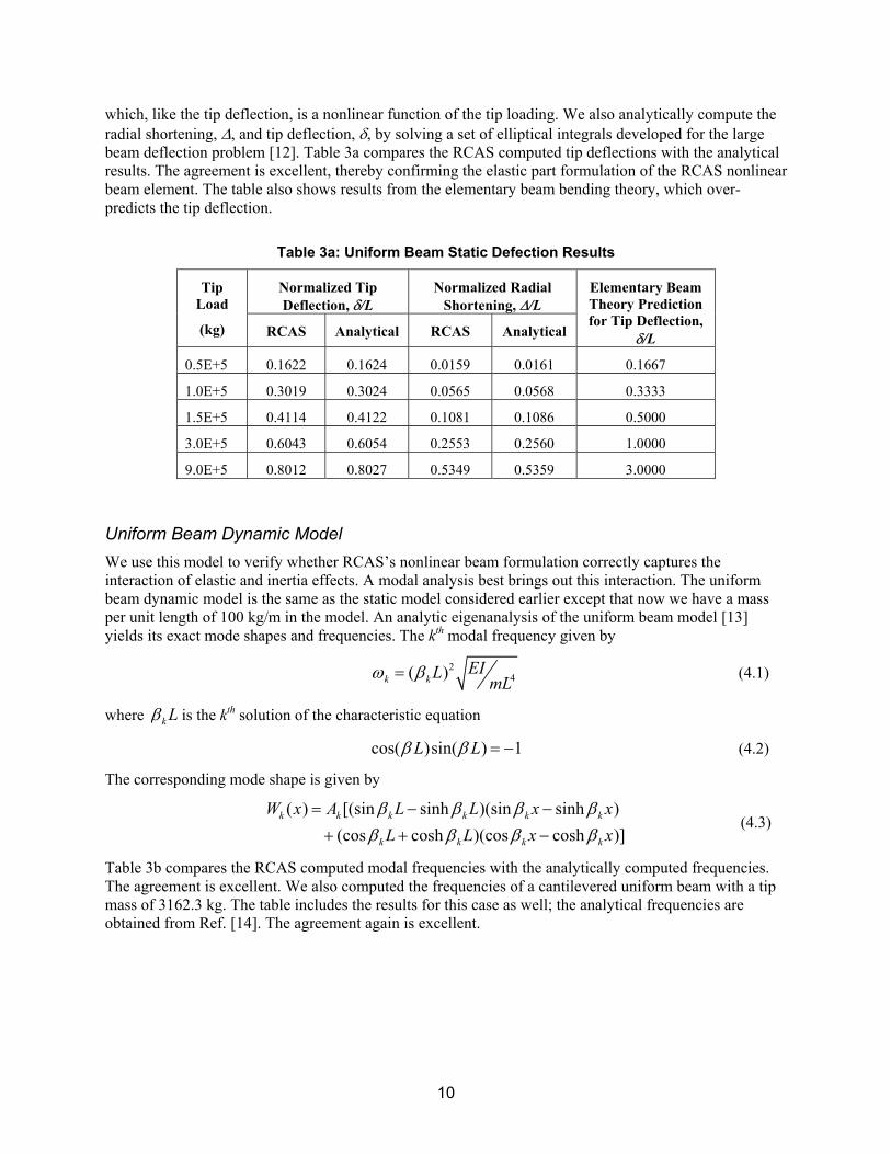
Uniform Beam Static Model An RCAS uniform beam model is built using eight nonlinear beam elements. The beam length, L, is 31.623 meters, and its cross-sectional flexural stiffness, EI, is 108 N-m2. The beam is assumed inextensible axially. We apply a tip load of different magnitudes and find its nonlinear static response. The tip load remains unchanged in direction (perpendicular to the undeformed blade axis). Figure 1 shows the bent-beam deflection shapes computed by RCAS for different tip loads. Note the radial shortening

10

which, like the tip deflection, is a nonlinear function of the tip loading. We also analytically compute the radial shortening, ∆, and tip deflection, δ, by solving a set of elliptical integrals developed for the large beam deflection problem [12]. Table 3a compares the RCAS computed tip deflections with the analytical results. The agreement is excellent, thereby confirming the elastic part formulation of the RCAS nonlinear beam element. The table also shows results from the elementary beam bending theory, which over-predicts the tip deflection.

Table 3a: Uniform Beam Static Defection Results

Normalized Tip Deflection, δ/L

Normalized Radial Shortening, ∆/L

Tip Load

(kg) RCAS Analytical RCAS Analytical

Elementary Beam Theory Prediction for Tip Deflection,

δ/L

0.5E+5 0.1622 0.1624 0.0159 0.0161 0.1667

1.0E+5 0.3019 0.3024 0.0565 0.0568 0.3333

1.5E+5 0.4114 0.4122 0.1081 0.1086 0.5000

3.0E+5 0.6043 0.6054 0.2553 0.2560 1.0000

9.0E+5 0.8012 0.8027 0.5349 0.5359 3.0000

Uniform Beam Dynamic Model We use this model to verify whether RCAS’s nonlinear beam formulation correctly captures the interaction of elastic and inertia effects. A modal analysis best brings out this interaction. The uniform beam dynamic model is the same as the static model considered earlier except that now we have a mass per unit length of 100 kg/m in the model. An analytic eigenanalysis of the uniform beam model [13] yields its exact mode shapes and frequencies. The kth modal frequency given by

24( )k k

EIL mLω β= (4.1)

where k Lβ is the kth solution of the characteristic equation

cos( )sin( ) 1L Lβ β = − (4.2)

The corresponding mode shape is given by

( ) [(sin sinh )(sin sinh )

(cos cosh )(cos cosh )]k k k k k k

k k k k

W x A L L x xL L x x

β β β ββ β β β

= − −+ + −

(4.3)

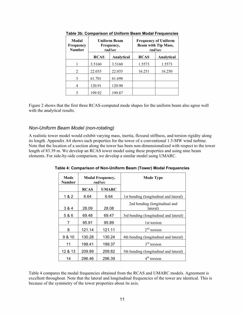
Table 3b compares the RCAS computed modal frequencies with the analytically computed frequencies. The agreement is excellent. We also computed the frequencies of a cantilevered uniform beam with a tip mass of 3162.3 kg. The table includes the results for this case as well; the analytical frequencies are obtained from Ref. [14]. The agreement again is excellent.

11

Table 3b: Comparison of Uniform Beam Modal Frequencies Uniform Beam

Frequency, rad/sec

Frequency of Uniform Beam with Tip Mass,

rad/sec

Modal Frequency Number

RCAS Analytical RCAS Analytical

1 3.5160 3.5160 1.5573 1.5573

2 22.035 22.035 16.251 16.250

3 61.701 61.698

4 120.91 120.90

5 199.92 199.87

Figure 2 shows that the first three RCAS-computed mode shapes for the uniform beam also agree well with the analytical results.

Non-Uniform Beam Model (non-rotating) A realistic tower model would exhibit varying mass, inertia, flexural stiffness, and torsion rigidity along its length. Appendix A4 shows such properties for the tower of a conventional 1.5-MW wind turbine. Note that the location of a section along the tower has been non-dimensionalized with respect to the tower length of 83.39 m. We develop an RCAS tower model using these properties and using nine beam elements. For side-by-side comparison, we develop a similar model using UMARC.

Table 4: Comparison of Non-Uniform Beam (Tower) Modal Frequencies

Mode Number

Modal Frequency, rad/sec

RCAS UMARC

Mode Type

1 & 2 6.64 6.64 1st bending (longitudinal and lateral)

3 & 4 28.09 28.08 2nd bending (longitudinal and

lateral)

5 & 6 69.48 69.47 3rd bending (longitudinal and lateral)

7 95.91 95.89 1st torsion

8 121.14 121.11 2nd torsion

9 & 10 130.28 130.24 4th bending (longitudinal and lateral)

11 199.41 199.37 3rd torsion

12 & 13 209.89 209.82 5th bending (longitudinal and lateral)

14 296.46 296.39 4th torsion

Table 4 compares the modal frequencies obtained from the RCAS and UMARC models. Agreement is excellent throughout. Note that the lateral and longitudinal frequencies of the tower are identical. This is because of the symmetry of the tower properties about its axis.

12

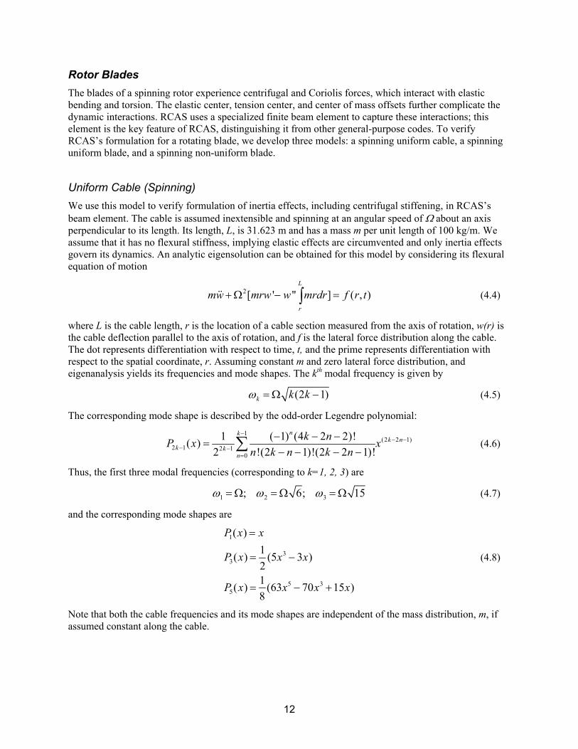
Rotor Blades The blades of a spinning rotor experience centrifugal and Coriolis forces, which interact with elastic bending and torsion. The elastic center, tension center, and center of mass offsets further complicate the dynamic interactions. RCAS uses a specialized finite beam element to capture these interactions; this element is the key feature of RCAS, distinguishing it from other general-purpose codes. To verify RCAS’s formulation for a rotating blade, we develop three models: a spinning uniform cable, a spinning uniform blade, and a spinning non-uniform blade.

Uniform Cable (Spinning) We use this model to verify formulation of inertia effects, including centrifugal stiffening, in RCAS’s beam element. The cable is assumed inextensible and spinning at an angular speed of Ω about an axis perpendicular to its length. Its length, L, is 31.623 m and has a mass m per unit length of 100 kg/m. We assume that it has no flexural stiffness, implying elastic effects are circumvented and only inertia effects govern its dynamics. An analytic eigensolution can be obtained for this model by considering its flexural equation of motion

2[ ' '' ] ( , )L

r

mw mrw w mrdr f r t+ Ω − =∫&& (4.4)

where L is the cable length, r is the location of a cable section measured from the axis of rotation, w(r) is the cable deflection parallel to the axis of rotation, and f is the lateral force distribution along the cable. The dot represents differentiation with respect to time, t, and the prime represents differentiation with respect to the spatial coordinate, r. Assuming constant m and zero lateral force distribution, and eigenanalysis yields its frequencies and mode shapes. The kth modal frequency is given by

(2 1)k k kω = Ω − (4.5)

The corresponding mode shape is described by the odd-order Legendre polynomial:

1

(2 2 1)2 1 2 1

0

1 ( 1) (4 2 2)!( )2 !(2 1)!(2 2 1)!

nkk n

k kn

k nP x xn k n k n

−− −

− −=

− − −=

− − − −∑ (4.6)

Thus, the first three modal frequencies (corresponding to k=1, 2, 3) are

1 2 3; 6; 15ω ω ω= Ω = Ω = Ω (4.7)

and the corresponding mode shapes are

1

33

5 35

( )1( ) (5 3 )21( ) (63 70 15 )8

P x x

P x x x

P x x x x

=

= −

= − +

(4.8)

Note that both the cable frequencies and its mode shapes are independent of the mass distribution, m, if assumed constant along the cable.

13

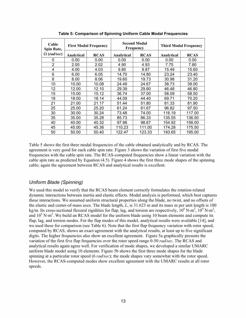
Table 5: Comparison of Spinning Uniform Cable Modal Frequencies

First Modal Frequency Second Modal Frequency Third Modal Frequency Cable

Spin Rate, Ω (rad/sec) Analytical RCAS Analytical RCAS Analytical RCAS

0 0.00 0.00 0.00 0.00 0.00 0.00 2 2.00 2.02 4.90 4.93 7.75 7.80 4 4.00 4.03 9.80 9.87 15.49 15.60 6 6.00 6.05 14.70 14.80 23.24 23.40 8 8.00 8.06 19.60 19.73 30.98 31.20 10 10.00 10.08 24.49 24.67 38.73 39.00 12 12.00 12.10 29.39 29.60 46.48 46.80 15 15.00 15.12 36.74 37.00 58.09 58.50 18 18.00 18.14 44.09 44.40 69.71 70.20 21 21.00 21.17 51.44 51.80 81.33 81.90 25 25.00 25.20 61.24 61.67 96.82 97.50 30 30.00 30.24 73.48 74.00 116.19 117.00 35 35.00 35.28 85.73 86.33 135.55 136.50 40 40.00 40.32 97.98 98.67 154.92 156.00 45 45.00 45.36 110.23 111.00 174.28 175.50 50 50.00 50.40 122.47 123.33 193.65 195.00

Table 5 shows the first three modal frequencies of the cable obtained analytically and by RCAS. The agreement is very good for each cable spin rate. Figure 3 shows the variation of first five modal frequencies with the cable spin rate. The RCAS-computed frequencies show a linear variation with the cable spin rate as predicted by Equation (4.5). Figure 4 shows the first three mode shapes of the spinning cable; again the agreement between RCAS and analytical results is excellent.

Uniform Blade (Spinning) We used this model to verify that the RCAS beam element correctly formulates the rotation-related dynamic interactions between inertia and elastic effects. Modal analysis is performed, which best captures these interactions. We assumed uniform structural properties along the blade, no twist, and no offsets of the elastic and center-of-mass axes. The blade length, L, is 31.623 m and its mass m per unit length is 100 kg/m. Its cross-sectional flexural rigidities for flap, lag, and torsion are respectively, 108 N-m2, 109 N-m2, and 105 N-m2. We build an RCAS model for the uniform blade using 10 beam elements and compute its flap, lag, and torsion modes. For the flap modes of this model, analytical results were available [14], and we used these for comparison (see Table 6). Note that the first flap frequency variation with rotor speed, computed by RCAS, shows an exact agreement with the analytical results, at least up to five significant digits. The higher frequencies also show an excellent agreement. Figure 5a graphically presents the variation of the first five flap frequencies over the rotor speed range 0-50 rad/sec. The RCAS and analytical results again agree well. For verification of mode shapes, we developed a similar UMARC uniform blade model using 10 elements. Figure 5b shows the first three mode shapes for the blade spinning at a particular rotor speed (6 rad/sec); the mode shapes vary somewhat with the rotor speed. However, the RCAS-computed modes show excellent agreement with the UMARC results at all rotor speeds.

14

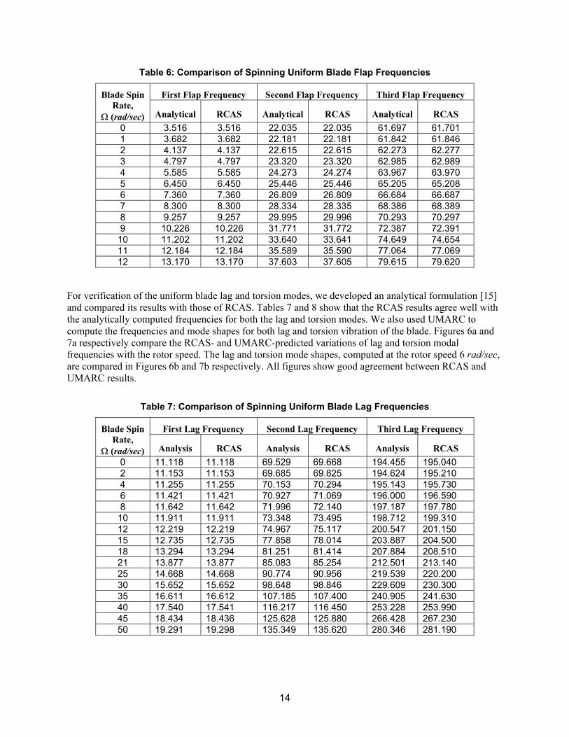
Table 6: Comparison of Spinning Uniform Blade Flap Frequencies

First Flap Frequency Second Flap Frequency Third Flap Frequency Blade Spin Rate,

Ω (rad/sec) Analytical RCAS Analytical RCAS Analytical RCAS 0 3.516 3.516 22.035 22.035 61.697 61.701 1 3.682 3.682 22.181 22.181 61.842 61.846 2 4.137 4.137 22.615 22.615 62.273 62.277 3 4.797 4.797 23.320 23.320 62.985 62.989 4 5.585 5.585 24.273 24.274 63.967 63.970 5 6.450 6.450 25.446 25.446 65.205 65.208 6 7.360 7.360 26.809 26.809 66.684 66.687 7 8.300 8.300 28.334 28.335 68.386 68.389 8 9.257 9.257 29.995 29.996 70.293 70.297 9 10.226 10.226 31.771 31.772 72.387 72.391 10 11.202 11.202 33.640 33.641 74.649 74.654 11 12.184 12.184 35.589 35.590 77.064 77.069 12 13.170 13.170 37.603 37.605 79.615 79.620

For verification of the uniform blade lag and torsion modes, we developed an analytical formulation [15] and compared its results with those of RCAS. Tables 7 and 8 show that the RCAS results agree well with the analytically computed frequencies for both the lag and torsion modes. We also used UMARC to compute the frequencies and mode shapes for both lag and torsion vibration of the blade. Figures 6a and 7a respectively compare the RCAS- and UMARC-predicted variations of lag and torsion modal frequencies with the rotor speed. The lag and torsion mode shapes, computed at the rotor speed 6 rad/sec, are compared in Figures 6b and 7b respectively. All figures show good agreement between RCAS and UMARC results.

Table 7: Comparison of Spinning Uniform Blade Lag Frequencies

First Lag Frequency Second Lag Frequency Third Lag Frequency Blade Spin Rate,

Ω (rad/sec) Analysis RCAS Analysis RCAS Analysis RCAS 0 11.118 11.118 69.529 69.668 194.455 195.040 2 11.153 11.153 69.685 69.825 194.624 195.210 4 11.255 11.255 70.153 70.294 195.143 195.730 6 11.421 11.421 70.927 71.069 196.000 196.590 8 11.642 11.642 71.996 72.140 197.187 197.780 10 11.911 11.911 73.348 73.495 198.712 199.310 12 12.219 12.219 74.967 75.117 200.547 201.150 15 12.735 12.735 77.858 78.014 203.887 204.500 18 13.294 13.294 81.251 81.414 207.884 208.510 21 13.877 13.877 85.083 85.254 212.501 213.140 25 14.668 14.668 90.774 90.956 219.539 220.200 30 15.652 15.652 98.648 98.846 229.609 230.300 35 16.611 16.612 107.185 107.400 240.905 241.630 40 17.540 17.541 116.217 116.450 253.228 253.990 45 18.434 18.436 125.628 125.880 266.428 267.230 50 19.291 19.298 135.349 135.620 280.346 281.190

15

Table 8: Comparison of Spinning Uniform Blade Torsion Frequencies

First Modal Frequency Second Modal Frequency Third Modal Frequency Blade Spin

Rate, Ω (rad/sec) Analysis RCAS Analysis RCAS Analysis RCAS

0 15.712 15.714 47.298 47.303 79.361 79.42 2 15.834 15.84 47.250 47.345 79.287 79.446 4 16.209 16.215 47.377 47.472 79.362 79.521 6 16.803 16.82 47.587 47.682 79.488 79.647 8 17.615 17.633 47.879 47.975 79.662 79.822 10 18.606 18.625 48.251 48.348 79.887 80.047 12 19.751 19.771 48.703 48.801 80.161 80.322 15 21.701 21.723 49.525 49.624 80.662 80.824 18 23.869 23.893 50.510 50.611 81.271 81.434 21 26.201 26.227 51.650 51.754 81.985 82.149 25 29.496 29.526 53.395 53.502 83.095 83.262 30 33.830 33.864 55.900 56.012 84.727 84.897 35 38.324 38.362 58.724 58.842 86.615 86.789 40 42.929 42.972 61.822 61.946 88.745 88.923 45 47.612 47.66 65.154 65.285 91.098 91.281 50 52.354 52.406 68.688 68.826 93.658 93.846

The fan plot in Figure 8 shows frequency variation of all the modal frequencies of the spinning blade with respect to the rotor speed.

Convergence study: We conducted a brief study to examine the effect of number of beam elements on the convergence of modal results. We first consider the case when the uniform blade is not rotating. Table 9 shows how RCAS-computed flap frequencies converge as the number of elements is increased from three to 10.

Table 9: Convergence of Flap Frequencies for the Uniform Blade (Non-Rotating)

Mode 1st flap 2nd flap 3rd flap 4th flap 5th flap

No. of Elements

RCAS ADAMS RCAS ADAMS RCAS ADAMS RCAS ADAMS RCAS ADAMS

3 3.516 3.529 22.12 20.70 62.33 50.28 139.35 79.72 260.34 100.56 5 3.516 3.521 22.05 21.55 61.96 57.22 122.61 103.32 202.82 153.62 7 3.516 3.519 22.04 21.79 61.86 59.35 121.21 111.39 203.27 173.95 8 3.516 3.518 22.04 21.84 61.75 59.88 121.23 113.49 201.57 179.48

10 3.516 3.517 22.04 21.91 61.74 60.52 121.08 116.06 201.14 186.37 12 3.517 21.95 60.88 117.50 190.30 15 3.517 21.98 61.17 118.69 193.62 20 3.516 22.00 61.39 119.64 196.27

For the first three flap modes, note that three elements suffice to yield frequencies within 1% accuracy. For five modes, we need eight elements to get the same accuracy. For comparison, we conducted a similar study using ADAMS. ADAMS results, especially for the higher modes, converge rather slowly. If we use 20 elements, the first two modes do converge within 1%. However, for higher modes, ADAMS would need more elements to yield the same accuracy. Table 10 presents convergence study results for the same blade spinning at 12 rad/sec. All five modes converge within 0.2% if we use 10 elements. No results are shown using ADAMS because it lacks a built-in linearization capability for a spinning blade.

16

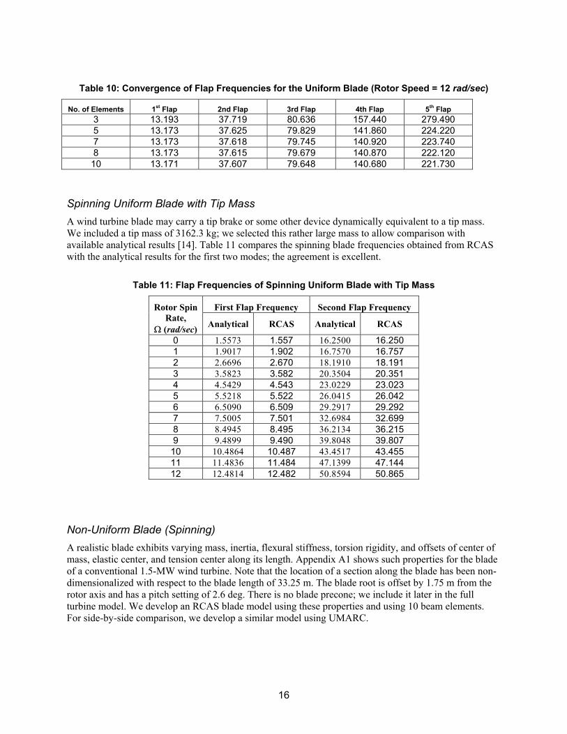
Table 10: Convergence of Flap Frequencies for the Uniform Blade (Rotor Speed = 12 rad/sec)

No. of Elements 1st Flap 2nd Flap 3rd Flap 4th Flap 5th Flap 3 13.193 37.719 80.636 157.440 279.490 5 13.173 37.625 79.829 141.860 224.220 7 13.173 37.618 79.745 140.920 223.740 8 13.173 37.615 79.679 140.870 222.120 10 13.171 37.607 79.648 140.680 221.730

Spinning Uniform Blade with Tip Mass A wind turbine blade may carry a tip brake or some other device dynamically equivalent to a tip mass. We included a tip mass of 3162.3 kg; we selected this rather large mass to allow comparison with available analytical results [14]. Table 11 compares the spinning blade frequencies obtained from RCAS with the analytical results for the first two modes; the agreement is excellent.

Table 11: Flap Frequencies of Spinning Uniform Blade with Tip Mass

First Flap Frequency Second Flap Frequency Rotor Spin Rate,

Ω (rad/sec) Analytical RCAS Analytical RCAS

0 1.5573 1.557 16.2500 16.250 1 1.9017 1.902 16.7570 16.757 2 2.6696 2.670 18.1910 18.191 3 3.5823 3.582 20.3504 20.351 4 4.5429 4.543 23.0229 23.023 5 5.5218 5.522 26.0415 26.042 6 6.5090 6.509 29.2917 29.292 7 7.5005 7.501 32.6984 32.699 8 8.4945 8.495 36.2134 36.215 9 9.4899 9.490 39.8048 39.807 10 10.4864 10.487 43.4517 43.455 11 11.4836 11.484 47.1399 47.144 12 12.4814 12.482 50.8594 50.865

Non-Uniform Blade (Spinning) A realistic blade exhibits varying mass, inertia, flexural stiffness, torsion rigidity, and offsets of center of mass, elastic center, and tension center along its length. Appendix A1 shows such properties for the blade of a conventional 1.5-MW wind turbine. Note that the location of a section along the blade has been non-dimensionalized with respect to the blade length of 33.25 m. The blade root is offset by 1.75 m from the rotor axis and has a pitch setting of 2.6 deg. There is no blade precone; we include it later in the full turbine model. We develop an RCAS blade model using these properties and using 10 beam elements. For side-by-side comparison, we develop a similar model using UMARC.

17

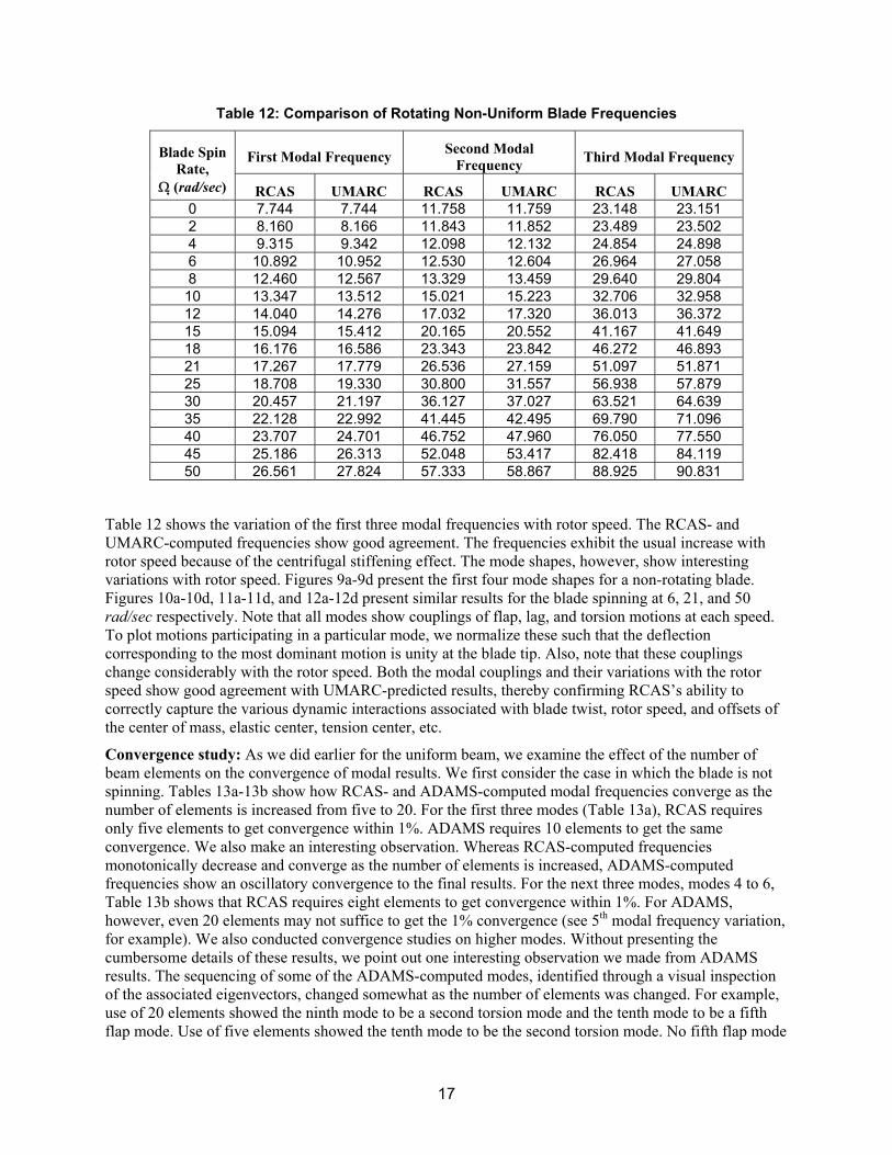
Table 12: Comparison of Rotating Non-Uniform Blade Frequencies

First Modal Frequency Second Modal Frequency Third Modal Frequency Blade Spin

Rate, Ω (rad/sec) RCAS UMARC RCAS UMARC RCAS UMARC

0 7.744 7.744 11.758 11.759 23.148 23.151 2 8.160 8.166 11.843 11.852 23.489 23.502 4 9.315 9.342 12.098 12.132 24.854 24.898 6 10.892 10.952 12.530 12.604 26.964 27.058 8 12.460 12.567 13.329 13.459 29.640 29.804 10 13.347 13.512 15.021 15.223 32.706 32.958 12 14.040 14.276 17.032 17.320 36.013 36.372 15 15.094 15.412 20.165 20.552 41.167 41.649 18 16.176 16.586 23.343 23.842 46.272 46.893 21 17.267 17.779 26.536 27.159 51.097 51.871 25 18.708 19.330 30.800 31.557 56.938 57.879 30 20.457 21.197 36.127 37.027 63.521 64.639 35 22.128 22.992 41.445 42.495 69.790 71.096 40 23.707 24.701 46.752 47.960 76.050 77.550 45 25.186 26.313 52.048 53.417 82.418 84.119 50 26.561 27.824 57.333 58.867 88.925 90.831

Table 12 shows the variation of the first three modal frequencies with rotor speed. The RCAS- and UMARC-computed frequencies show good agreement. The frequencies exhibit the usual increase with rotor speed because of the centrifugal stiffening effect. The mode shapes, however, show interesting variations with rotor speed. Figures 9a-9d present the first four mode shapes for a non-rotating blade. Figures 10a-10d, 11a-11d, and 12a-12d present similar results for the blade spinning at 6, 21, and 50 rad/sec respectively. Note that all modes show couplings of flap, lag, and torsion motions at each speed. To plot motions participating in a particular mode, we normalize these such that the deflection corresponding to the most dominant motion is unity at the blade tip. Also, note that these couplings change considerably with the rotor speed. Both the modal couplings and their variations with the rotor speed show good agreement with UMARC-predicted results, thereby confirming RCAS’s ability to correctly capture the various dynamic interactions associated with blade twist, rotor speed, and offsets of the center of mass, elastic center, tension center, etc.

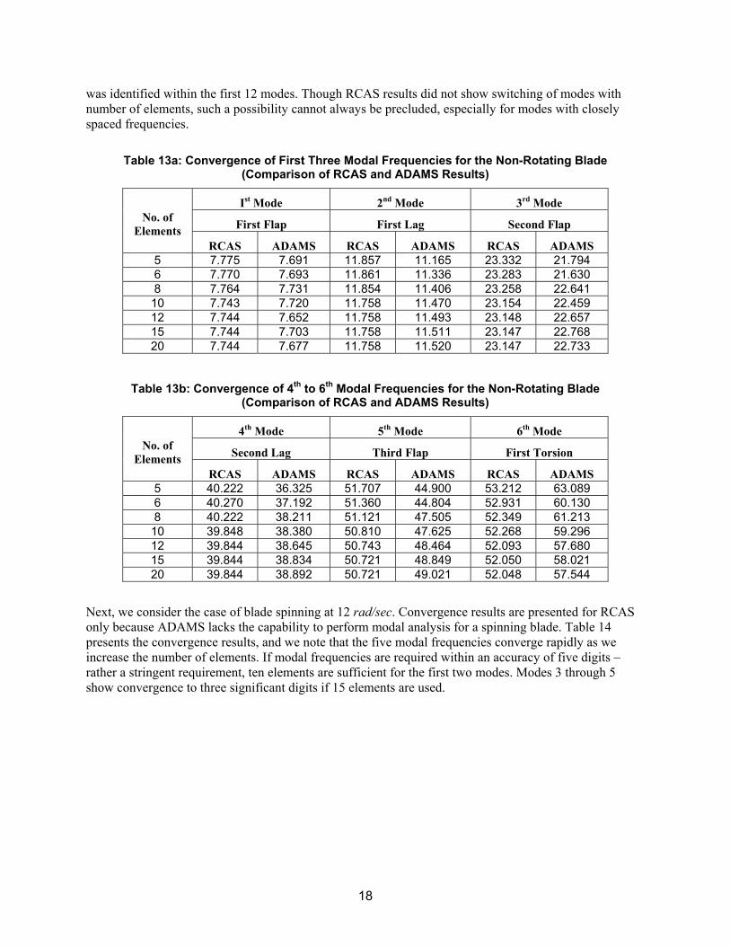
Convergence study: As we did earlier for the uniform beam, we examine the effect of the number of beam elements on the convergence of modal results. We first consider the case in which the blade is not spinning. Tables 13a-13b show how RCAS- and ADAMS-computed modal frequencies converge as the number of elements is increased from five to 20. For the first three modes (Table 13a), RCAS requires only five elements to get convergence within 1%. ADAMS requires 10 elements to get the same convergence. We also make an interesting observation. Whereas RCAS-computed frequencies monotonically decrease and converge as the number of elements is increased, ADAMS-computed frequencies show an oscillatory convergence to the final results. For the next three modes, modes 4 to 6, Table 13b shows that RCAS requires eight elements to get convergence within 1%. For ADAMS, however, even 20 elements may not suffice to get the 1% convergence (see 5th modal frequency variation, for example). We also conducted convergence studies on higher modes. Without presenting the cumbersome details of these results, we point out one interesting observation we made from ADAMS results. The sequencing of some of the ADAMS-computed modes, identified through a visual inspection of the associated eigenvectors, changed somewhat as the number of elements was changed. For example, use of 20 elements showed the ninth mode to be a second torsion mode and the tenth mode to be a fifth flap mode. Use of five elements showed the tenth mode to be the second torsion mode. No fifth flap mode

18

was identified within the first 12 modes. Though RCAS results did not show switching of modes with number of elements, such a possibility cannot always be precluded, especially for modes with closely spaced frequencies.

Table 13a: Convergence of First Three Modal Frequencies for the Non-Rotating Blade (Comparison of RCAS and ADAMS Results)

Ist Mode 2nd Mode 3rd Mode

First Flap First Lag Second Flap No. of Elements

RCAS ADAMS RCAS ADAMS RCAS ADAMS 5 7.775 7.691 11.857 11.165 23.332 21.794 6 7.770 7.693 11.861 11.336 23.283 21.630 8 7.764 7.731 11.854 11.406 23.258 22.641 10 7.743 7.720 11.758 11.470 23.154 22.459 12 7.744 7.652 11.758 11.493 23.148 22.657 15 7.744 7.703 11.758 11.511 23.147 22.768 20 7.744 7.677 11.758 11.520 23.147 22.733

Table 13b: Convergence of 4th to 6th Modal Frequencies for the Non-Rotating Blade (Comparison of RCAS and ADAMS Results)

4th Mode 5th Mode 6th Mode

Second Lag Third Flap First Torsion No. of Elements

RCAS ADAMS RCAS ADAMS RCAS ADAMS 5 40.222 36.325 51.707 44.900 53.212 63.089 6 40.270 37.192 51.360 44.804 52.931 60.130 8 40.222 38.211 51.121 47.505 52.349 61.213 10 39.848 38.380 50.810 47.625 52.268 59.296 12 39.844 38.645 50.743 48.464 52.093 57.680 15 39.844 38.834 50.721 48.849 52.050 58.021 20 39.844 38.892 50.721 49.021 52.048 57.544

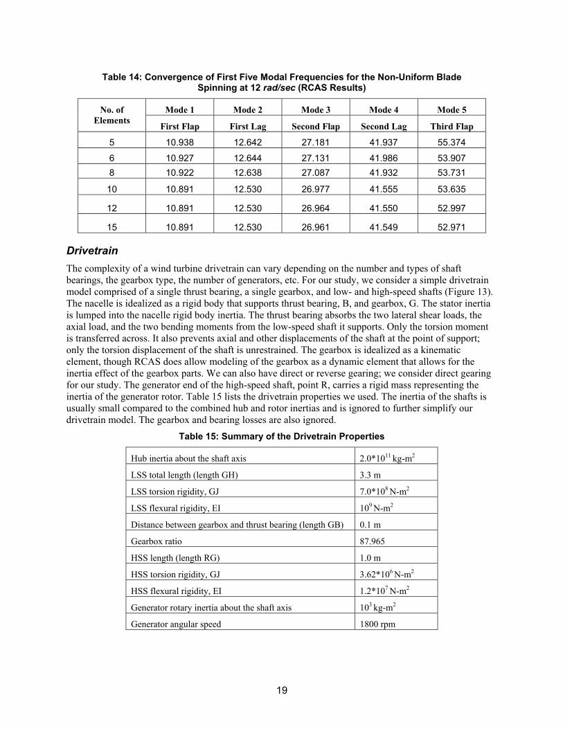
Next, we consider the case of blade spinning at 12 rad/sec. Convergence results are presented for RCAS only because ADAMS lacks the capability to perform modal analysis for a spinning blade. Table 14 presents the convergence results, and we note that the five modal frequencies converge rapidly as we increase the number of elements. If modal frequencies are required within an accuracy of five digits – rather a stringent requirement, ten elements are sufficient for the first two modes. Modes 3 through 5 show convergence to three significant digits if 15 elements are used.

19

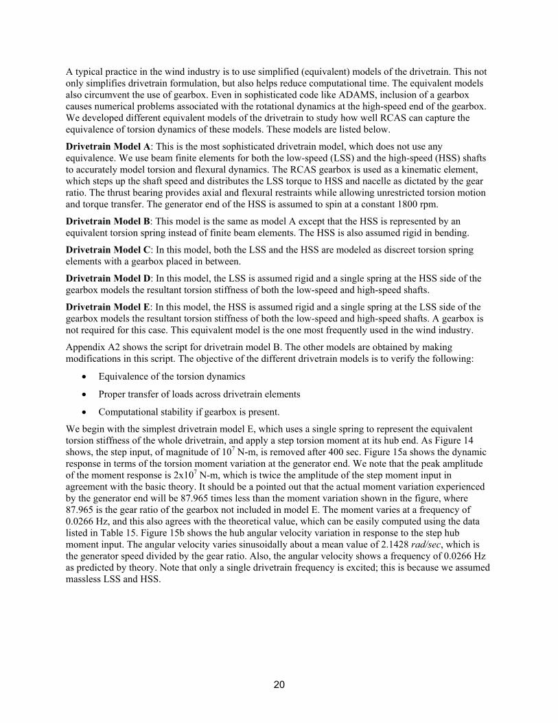
Table 14: Convergence of First Five Modal Frequencies for the Non-Uniform Blade Spinning at 12 rad/sec (RCAS Results)

Mode 1 Mode 2 Mode 3 Mode 4 Mode 5 No. of Elements First Flap First Lag Second Flap Second Lag Third Flap

5 10.938 12.642 27.181 41.937 55.374

6 10.927 12.644 27.131 41.986 53.907 8 10.922 12.638 27.087 41.932 53.731

10 10.891 12.530 26.977 41.555 53.635

12 10.891 12.530 26.964 41.550 52.997

15 10.891 12.530 26.961 41.549 52.971

Drivetrain The complexity of a wind turbine drivetrain can vary depending on the number and types of shaft bearings, the gearbox type, the number of generators, etc. For our study, we consider a simple drivetrain model comprised of a single thrust bearing, a single gearbox, and low- and high-speed shafts (Figure 13). The nacelle is idealized as a rigid body that supports thrust bearing, B, and gearbox, G. The stator inertia is lumped into the nacelle rigid body inertia. The thrust bearing absorbs the two lateral shear loads, the axial load, and the two bending moments from the low-speed shaft it supports. Only the torsion moment is transferred across. It also prevents axial and other displacements of the shaft at the point of support; only the torsion displacement of the shaft is unrestrained. The gearbox is idealized as a kinematic element, though RCAS does allow modeling of the gearbox as a dynamic element that allows for the inertia effect of the gearbox parts. We can also have direct or reverse gearing; we consider direct gearing for our study. The generator end of the high-speed shaft, point R, carries a rigid mass representing the inertia of the generator rotor. Table 15 lists the drivetrain properties we used. The inertia of the shafts is usually small compared to the combined hub and rotor inertias and is ignored to further simplify our drivetrain model. The gearbox and bearing losses are also ignored.

Table 15: Summary of the Drivetrain Properties

Hub inertia about the shaft axis 2.0*1011 kg-m2

LSS total length (length GH) 3.3 m

LSS torsion rigidity, GJ 7.0*108 N-m2

LSS flexural rigidity, EI 109 N-m2

Distance between gearbox and thrust bearing (length GB) 0.1 m

Gearbox ratio 87.965

HSS length (length RG) 1.0 m

HSS torsion rigidity, GJ 3.62*106 N-m2

HSS flexural rigidity, EI 1.2*107 N-m2

Generator rotary inertia about the shaft axis 103 kg-m2

Generator angular speed 1800 rpm

20

A typical practice in the wind industry is to use simplified (equivalent) models of the drivetrain. This not only simplifies drivetrain formulation, but also helps reduce computational time. The equivalent models also circumvent the use of gearbox. Even in sophisticated code like ADAMS, inclusion of a gearbox causes numerical problems associated with the rotational dynamics at the high-speed end of the gearbox. We developed different equivalent models of the drivetrain to study how well RCAS can capture the equivalence of torsion dynamics of these models. These models are listed below.

Drivetrain Model A: This is the most sophisticated drivetrain model, which does not use any equivalence. We use beam finite elements for both the low-speed (LSS) and the high-speed (HSS) shafts to accurately model torsion and flexural dynamics. The RCAS gearbox is used as a kinematic element, which steps up the shaft speed and distributes the LSS torque to HSS and nacelle as dictated by the gear ratio. The thrust bearing provides axial and flexural restraints while allowing unrestricted torsion motion and torque transfer. The generator end of the HSS is assumed to spin at a constant 1800 rpm.

Drivetrain Model B: This model is the same as model A except that the HSS is represented by an equivalent torsion spring instead of finite beam elements. The HSS is also assumed rigid in bending.

Drivetrain Model C: In this model, both the LSS and the HSS are modeled as discreet torsion spring elements with a gearbox placed in between.

Drivetrain Model D: In this model, the LSS is assumed rigid and a single spring at the HSS side of the gearbox models the resultant torsion stiffness of both the low-speed and high-speed shafts.

Drivetrain Model E: In this model, the HSS is assumed rigid and a single spring at the LSS side of the gearbox models the resultant torsion stiffness of both the low-speed and high-speed shafts. A gearbox is not required for this case. This equivalent model is the one most frequently used in the wind industry.

Appendix A2 shows the script for drivetrain model B. The other models are obtained by making modifications in this script. The objective of the different drivetrain models is to verify the following:

• Equivalence of the torsion dynamics

• Proper transfer of loads across drivetrain elements

• Computational stability if gearbox is present.

We begin with the simplest drivetrain model E, which uses a single spring to represent the equivalent torsion stiffness of the whole drivetrain, and apply a step torsion moment at its hub end. As Figure 14 shows, the step input, of magnitude of 107 N-m, is removed after 400 sec. Figure 15a shows the dynamic response in terms of the torsion moment variation at the generator end. We note that the peak amplitude of the moment response is 2x107 N-m, which is twice the amplitude of the step moment input in agreement with the basic theory. It should be a pointed out that the actual moment variation experienced by the generator end will be 87.965 times less than the moment variation shown in the figure, where 87.965 is the gear ratio of the gearbox not included in model E. The moment varies at a frequency of 0.0266 Hz, and this also agrees with the theoretical value, which can be easily computed using the data listed in Table 15. Figure 15b shows the hub angular velocity variation in response to the step hub moment input. The angular velocity varies sinusoidally about a mean value of 2.1428 rad/sec, which is the generator speed divided by the gear ratio. Also, the angular velocity shows a frequency of 0.0266 Hz as predicted by theory. Note that only a single drivetrain frequency is excited; this is because we assumed massless LSS and HSS.

21

We apply the same step input hub moment to all the drivetrain models and use RCAS to predict the hub- and generator-end responses. Figure 16a compares the generator-end moment variation experienced by the different models (note we have divided the moment variation result for model E by the gear ratio as required). Figure 16b compares the angular velocity variation at hub end of the different models. All models show excellent agreement, thereby confirming RCAS’s ability to analyze the equivalent models correctly. Note that we modeled the LSS and HSS as massless elements for the purpose of verification. Also note that the results for model A are missing. This is because this model experienced numerical instability and no results could be obtained. While the finite element modeling of the LSS yields correct results, as evidenced by model B, finite element modeling of the rapidly spinning HSS leads to numerical problems. The problem was reported to ART and the AeroFlightDynamics Directorate (AFDD) and they recently fixed it; we will verify the updated drivetrain model in the near future.

Any of the five equivalent models describes above would suffice if we were interested in the torsional dynamics of an isolated drivetrain only. Model E, the only model that does not include the gearbox and the one most frequently used in ADAMS, would, however, not be adequate if we were interested in detailed dynamics loads, e.g., in the gyroscopic pitching moments associated with the yawing of the drivetrain. Model C or D may be adequate if the drivetrain shaft that is light in comparison to the rotor and generator is also stiff in bending. Otherwise, one must use model A or model B.

Drivetrain Control Exercise As mentioned in Section 2, RCAS has a graphical user interface (CSGE) to develop a control system of arbitrary complexity and integrate it with the RCAS structural or aeroelastic model. We use the CSGE to develop a simple proportional-integral (PI) controller and integrate it with the drivetrain model described above. The objective is simply to check the workability of CSGE-developed control model and its interface with RCAS. No attempt is made to verify or optimize controls.

Figure 17 shows the PI controller built using the CSGE. The interface between the CSGE controller and the RCAS drivetrain model is provided by the interface script komg.cmd (see Appendix A3). Before applying the control, we find the trim solution for the drivetrain, which yields an LSS rotational speed of 1.5 rad/sec. We then set the controller on with a proportional control gain of 1000, and integral control gain of 70,000. The target speed is 2.14 rad/sec (20.44 rpm). Figure 18a shows the LSS speed response following the application of control; the target speed is attained within about 12 seconds. Figure 18b shows the associated drivetrain torque commanded by the controller. Figures 19a and 19b show similar plots when the proportional gain is set to 10,000 and the integral gain to 20,000. In these cases, there is no oscillatory response and also less overshoot; however, it takes about 25 seconds before the desired LSS speed is attained.

One of the main motivations to acquire RCAS is to use it for state-space controls. However, we did not have time to learn CSGE well enough to exercise this option. We may try this in the future.

Full Wind Turbine System Finally, we focus on the full horizontal-axis wind turbine (HAWT). The structural configuration of a HAWT can vary depending on the type of hub (teetering, articulated, rigid, etc.), blade-pitch and yaw mechanisms, drivetrain complexity, tower construction, and the construction and geometry of the blades. For our studies, we consider a conventional 1.5-MW HAWT design. Table 16 summarizes its main properties. The rotor blade is straight, tapered, and twisted, with isotopic structural properties (see Appendix A1 for the blade properties). The drivetrain consists of a single thrust bearing, a single gearbox, and low- and high-speed shafts (Figure 13). The nacelle supports thrust bearing, B, and gearbox, G. The inertia of the stator and other non-rotating drivetrain parts are lumped into the inertia of the nacelle,

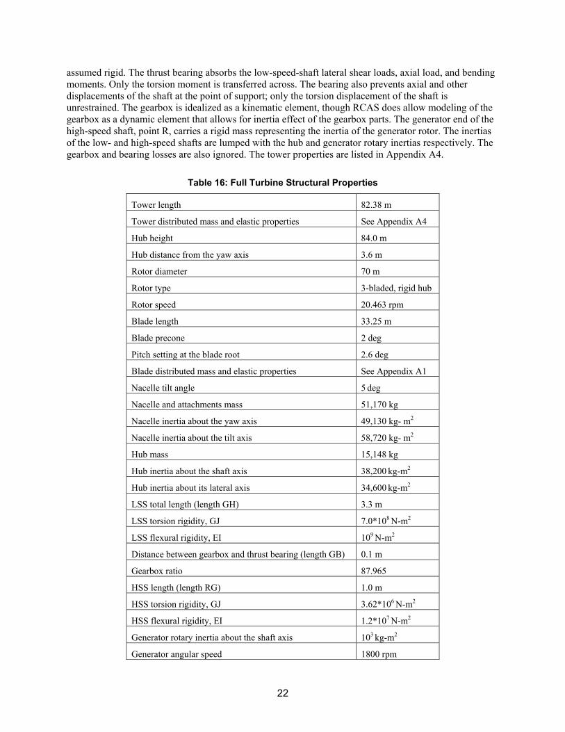
22

assumed rigid. The thrust bearing absorbs the low-speed-shaft lateral shear loads, axial load, and bending moments. Only the torsion moment is transferred across. The bearing also prevents axial and other displacements of the shaft at the point of support; only the torsion displacement of the shaft is unrestrained. The gearbox is idealized as a kinematic element, though RCAS does allow modeling of the gearbox as a dynamic element that allows for inertia effect of the gearbox parts. The generator end of the high-speed shaft, point R, carries a rigid mass representing the inertia of the generator rotor. The inertias of the low- and high-speed shafts are lumped with the hub and generator rotary inertias respectively. The gearbox and bearing losses are also ignored. The tower properties are listed in Appendix A4.

Table 16: Full Turbine Structural Properties

Tower length 82.38 m

Tower distributed mass and elastic properties See Appendix A4

Hub height 84.0 m

Hub distance from the yaw axis 3.6 m

Rotor diameter 70 m

Rotor type 3-bladed, rigid hub

Rotor speed 20.463 rpm

Blade length 33.25 m

Blade precone 2 deg

Pitch setting at the blade root 2.6 deg

Blade distributed mass and elastic properties See Appendix A1

Nacelle tilt angle 5 deg

Nacelle and attachments mass 51,170 kg

Nacelle inertia about the yaw axis 49,130 kg- m2

Nacelle inertia about the tilt axis 58,720 kg- m2

Hub mass 15,148 kg

Hub inertia about the shaft axis 38,200 kg-m2

Hub inertia about its lateral axis 34,600 kg-m2

LSS total length (length GH) 3.3 m

LSS torsion rigidity, GJ 7.0*108 N-m2

LSS flexural rigidity, EI 109 N-m2

Distance between gearbox and thrust bearing (length GB) 0.1 m

Gearbox ratio 87.965

HSS length (length RG) 1.0 m

HSS torsion rigidity, GJ 3.62*106 N-m2

HSS flexural rigidity, EI 1.2*107 N-m2

Generator rotary inertia about the shaft axis 103 kg-m2

Generator angular speed 1800 rpm

23

RCAS offers a number of analyses that may be performed on the full system model. However, all of these options cannot be directly verified for lack of parallel modeling and analyses required for side-by-side comparisons. First, no analytical formulation is available or possible for the full system. Second, ADAMS, the only general-purpose code available for side-by-side comparison, is limited to only two capabilities: parked-turbine-modal-analysis and simulation. Jonkman [4] has already verified these capabilities of RCAS. Some simplifications, however, were required in the full system model to permit comparison with FAST and ADAMS. The main simplification was in the drivetrain model; the whole drivetrain was modeled as a rigid shaft spinning at a constant speed and connected to the hub via a torsion spring.

For our studies, directed toward unique features of RCAS, these simplifications were not required and we developed a sophisticated full-system model in accordance with the properties listed in Table 16. However, we did make one simplification; the high-speed shaft was modeled as a torsion spring instead of a nonlinear beam-shaft element to avoid drivetrain numerical instability mentioned earlier. We then used this model to exercise features unique to RCAS (e.g., operating modes and stability analyses, multi-blade coordinate transformation, periodic state-space formulation, trim analysis, and modal reduction). Though none of these results is rigorously verifiable because of lack of analytical solutions or a computer code with similar capabilities, we present sample results to confirm the workability of select RCAS features that we believe will help advance design and analyses of wind turbines.

Operating Turbine Modes Our objective here is to exercise RCAS to generate a Coleman plot, which shows the variation of the system frequencies with the rotor speed. Such a plot provides insight into system dynamics and identifies potential resonance and instability regions. To obtain this plot, we use a feature of RCAS to handle multiple cases in a single run (in the current scenario, each rotor speed represents a single case). We consider a rotor speed range of 0-40 rad/sec, select 23 points in the range, and run RCAS to yield system frequencies, damping levels, and mode shapes at each of these points (rotor speeds). Figure 20a shows the system frequencies computed by RCAS at each rotor speed. The figure, however, does not quite show how a particular system mode and its associated frequency would vary with rotor speed. Identifying these trends usually requires time and expertise. One must examine the eigenvector associated with each frequency point, and then connect the points to identify these trends. RCAS, fortunately, offers an identification technique to automate this procedure. Figure 20b shows the plot RCAS generated using this option. Note, however, that each curve on this plot shows variation of frequency associated with a system degree of freedom, and not a participating system mode. Also, some of these degrees of freedom refer to a non-rotating frame, and some to a rotating frame. A physical understanding of system dynamics from this plot would be extremely difficult, if not impossible. For this, we need multi-blade coordinate (MBC) transformation.

Multi-Blade Coordinate Transformation MBC transforms the individual blade modes into a set of rotor modes, which look at the rotor blades collectively rather than individually. Multi-blade coordinates are easy to interpret, simplify the equations of motion, and govern the physical interactions of the rotor with the non-rotating part of the system. A full explanation of the MBC is beyond the scope of this report. One may refer to any book on rotorcraft dynamics for this purpose; Ref [16] is an excellent source.

We invoke the MBC option of RCAS and regenerate the frequencies’ fan plot. Figure 21a shows the dot plot, and Figure 21b shows the line plot obtained using RCAS’s modal identification option. The line plot

24

now takes on a more familiar look of a typical Coleman plot. An explanation of each curve on this plot is not the intent of this report. However, we would like to make an observation. Readers familiar with rotor dynamics may readily recognize the curve associated with the rotor in-plane first regressive mode, wherein the rotor blades oscillate in the plane of the rotor in a manner that causes the effective rotor center of mass to whirl in a direction opposite to that of the rotor angular velocity. This curve is shown as a solid line in the dot plot (Figure 21a). System eigenvectors were examined to identify this line. Figure 21b, obtained, however, shows that RCAS’s automated identification does not quite capture this line over the rotor speed range 0-1.9 Hz. The line segments AB, CD, and EF in fact should a make a single line AF, thereby making AFG a single curve representing the aforementioned regressive mode. Such misidentifications occur at other places also. Choosing more points (cases) to cover the rotor speed range can somewhat mitigate this problem. However, one must check eigenvectors to correct curves, especially near areas of frequency crossovers. RCAS’s automated identification feature, though, reduces manual examination of eigenvectors drastically.

Modal Reduction Modal reduction is an extremely useful capability of RCAS and offers many benefits. The two main benefits are the reduction of analysis time and the generation of high-fidelity low-order models for several applications, including controls design and analyses. RCAS allows arbitrary specification of modes for modal reduction. We tried the first 10 rotating-blade modes. The Coleman plot, generated after modal reduction, is shown in Figure 22. This looks very similar to the plot we obtained without modal reduction (Figure 21b). This shows that the ignored higher blade modes have little effect on the lower system modes of interest. The close similarity of the plots also verifies the correct implementation of the modal reduction feature in RCAS.

Next, we choose the first six blade modes for modal reduction. Figure 23 shows the resulting Coleman plot. This plot is very similar to the plot obtained using 10 modes, showing the efficacy of further modal reduction. However, the curves differ in the small vicinity of point R on the plot. RCAS’s automated modal identification obviously fails in this region. As mentioned earlier, RCAS does a good identification job for the most part, thereby saving an enormous amount of user time in the interpretation of modes. However, the user must exercise caution near frequency crossover regions and inspect system eigenvectors to correctly generate the frequency plots.

System Response Finally, we assess the RCAS computational time required for a simulation. Ref [4] noted that RCAS took an order-of-magnitude more time than ADAMS for a full-system simulation. It was also reported that the same number of degrees of freedom were used in both RCAS and ADAMS. Convergence studies on the isolated beam modal analysis, shown earlier in this section, suggest that RCAS, unlike ADAMS, may not require that many degrees of freedom to achieve a desired accuracy. This is because RCAS uses a specialized finite element to model elastic beams, allowing fewer elements to model the dynamics accurately. Accordingly, we performed several studies on the full turbine system to examine the effect of the number of finite elements on the accuracy and time taken for simulations. We also examined the effect of modal reduction and finite-element Gaussian points on the simulation time and accuracy. Presented below is a sample study.

We take the full system model described earlier, apply a time-varying load at the tip of one of its blades, and examine the response using different numbers of elements. The tip load is a follower force, always remaining normal to the local blade chord. Figure 24 shows time variation of the applied follower force applied over 49 seconds. The force is ramped up from zero to 10,000 N over the time interval 6.2-8.2

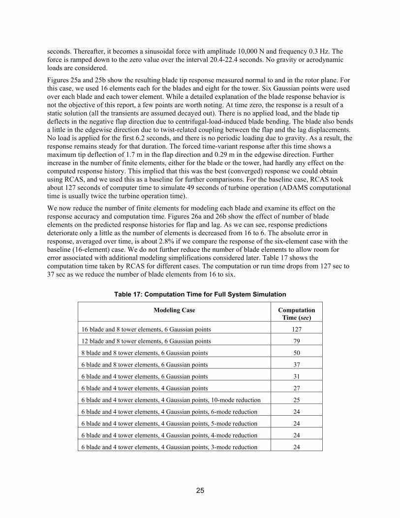
25

seconds. Thereafter, it becomes a sinusoidal force with amplitude 10,000 N and frequency 0.3 Hz. The force is ramped down to the zero value over the interval 20.4-22.4 seconds. No gravity or aerodynamic loads are considered.

Figures 25a and 25b show the resulting blade tip response measured normal to and in the rotor plane. For this case, we used 16 elements each for the blades and eight for the tower. Six Gaussian points were used over each blade and each tower element. While a detailed explanation of the blade response behavior is not the objective of this report, a few points are worth noting. At time zero, the response is a result of a static solution (all the transients are assumed decayed out). There is no applied load, and the blade tip deflects in the negative flap direction due to centrifugal-load-induced blade bending. The blade also bends a little in the edgewise direction due to twist-related coupling between the flap and the lag displacements. No load is applied for the first 6.2 seconds, and there is no periodic loading due to gravity. As a result, the response remains steady for that duration. The forced time-variant response after this time shows a maximum tip deflection of 1.7 m in the flap direction and 0.29 m in the edgewise direction. Further increase in the number of finite elements, either for the blade or the tower, had hardly any effect on the computed response history. This implied that this was the best (converged) response we could obtain using RCAS, and we used this as a baseline for further comparisons. For the baseline case, RCAS took about 127 seconds of computer time to simulate 49 seconds of turbine operation (ADAMS computational time is usually twice the turbine operation time).

We now reduce the number of finite elements for modeling each blade and examine its effect on the response accuracy and computation time. Figures 26a and 26b show the effect of number of blade elements on the predicted response histories for flap and lag. As we can see, response predictions deteriorate only a little as the number of elements is decreased from 16 to 6. The absolute error in response, averaged over time, is about 2.8% if we compare the response of the six-element case with the baseline (16-element) case. We do not further reduce the number of blade elements to allow room for error associated with additional modeling simplifications considered later. Table 17 shows the computation time taken by RCAS for different cases. The computation or run time drops from 127 sec to 37 sec as we reduce the number of blade elements from 16 to six.

Table 17: Computation Time for Full System Simulation

Modeling Case Computation Time (sec)

16 blade and 8 tower elements, 6 Gaussian points 127

12 blade and 8 tower elements, 6 Gaussian points 79

8 blade and 8 tower elements, 6 Gaussian points 50

6 blade and 8 tower elements, 6 Gaussian points 37

6 blade and 4 tower elements, 6 Gaussian points 31

6 blade and 4 tower elements, 4 Gaussian points 27

6 blade and 4 tower elements, 4 Gaussian points, 10-mode reduction 25

6 blade and 4 tower elements, 4 Gaussian points, 6-mode reduction 24

6 blade and 4 tower elements, 4 Gaussian points, 5-mode reduction 24

6 blade and 4 tower elements, 4 Gaussian points, 4-mode reduction 24

6 blade and 4 tower elements, 4 Gaussian points, 3-mode reduction 24

26

Next, we reduce the number of tower elements from eight to four. Figures 27a and 27b show that both the flap and lag responses deteriorate very little. The drop in accuracy, measured in terms of averaged absolute error, is about 0.85% as we move from eight to four tower elements. Figures 28a and 28b show that the effect of reducing Gaussian points from six to four, for both the blade and tower elements, also has little effect on the predicted flap and lag responses. The drop in accuracy is about 1.2%. Numerical instability resulted when we reduced the number of Gaussian points to two.

Finally, we performed modal reduction using the blade modes ranging from the first three to the first ten. Figures 29a and 29b show the resulting effect on the response predictions. The drop in response-prediction accuracy is about 1% when we use 10 modes, 3% when we use six modes, and 11% when we use three modes. Interestingly though, modal reduction does not yield much in terms of computational time saving (see Table 17). Modal reduction using 10 modes saves only 2 sec, using six modes saves 3 sec, and using four modes saves 4 sec. Further reduction in the number of modes does not yield any additional time saving.

Considering computation time versus accuracy, we reckon that a combination of six blade elements, four tower elements, four Gaussian points, and six modes would yield the best result for this simulation study. The response predictions resulting from this combination are compared with the baseline predictions in Figures 30a and 30b. The computational time saving is about 103 sec (24 versus 127 sec) with only a 4.8% drop in time-averaged accuracy for the flap response and 6.5% drop for the lag response.

We have presented results of a specific simulation study. We performed a few other studies covering simulation, trim, and stability analyses. The simulation results overall showed a similar trend in computation time versus accuracy. Reducing the number of blade elements had the maximum beneficial effect in terms of substantial time saving with little drop in accuracy. The trim analyses, usually very time consuming, particularly benefited from the reduction in the number of finite elements. Modal reduction, though yielding little time saving for trim and simulation, resulted in substantial computational time reduction for the modal and stability analyses. 5. Critique of RCAS Capabilities and User-Friendliness Verification results on the full system [4] showed close agreement between the RCAS and ADAMS results. Only slight discrepancies were noticed, for example in the blade torsion response. The slight discrepancies are understandable because RCAS uses a more sophisticated finite element approach compared to the lumped-mass approach used by ADAMS. Verification results presented in this report confirm this. Whenever analytical results were available for comparison, RCAS results showed slightly better agreement and faster convergence compared to ADAMS. Slightly better accuracy offered by RCAS, however, does not justify its adaptation for wind turbines. Its key strengths are its high-fidelity-modeling capability and its modeling and analysis features not offered by other general-purpose codes.

The high-fidelity modeling capability of RCAS is not directly verifiable. This is because existing codes do not have a similar capability to allow side-by-side comparisons. Note, for example, the full turbine RCAS model used in [4] was simplified to match modeling capabilities of ADAMS and FAST and make verification studies possible. In particular, the drivetrain was simplified; it was modeled as a single torsion spring. While for most applications such simplifications are justifiable, situations may arise wherein a high-fidelity model is desired. Examples include high-fidelity state-space modeling, understanding detailed drivetrain dynamics, and tracing detailed load-transfer mechanisms. The high-fidelity modeling capability of RCAS was verified at the component level in this report. Particular attention was paid to the elastic blade modeling. This is because most of the wind turbine components behave as elastic beams (tower, rotor blades, and drivetrain shafts). Verification results show that RCAS can model the elastic beam with a high degree of fidelity through a proper choice of number of elements, number of Gaussian integration points, and the number of modes for modal reduction. A verification of high-fidelity drivetrain models versus its equivalent models was also attempted. Results showed that

27

RCAS could accurately model the drivetrain dynamics, including transfer of dynamic loads from the gearbox and the thrust bearing to the nacelle, with one exception. It could not model a drivetrain with its high-speed-shaft modeled by beam-shaft finite elements. The high-speed shaft needs to be modeled as an equivalent spring on one side of the gearbox with the low-speed shaft modeled as a finite-element beam-shaft on the other side of the gearbox. ART members were notified of this problem, and they have just released a new version of RCAS, which allows finite element modeling of the high-speed shaft. However, care needs to be exercised in choosing the correct integration time step to accommodate high-frequency dynamics of the shaft at the generator end. Though preliminary results appear promising, we have not fully verified the new drivetrain implementation. It is worth mentioning here that the Aeroflightdynamics Directorate at NASA-Ames also had conducted some verification studies. Most of these studies were focused on the aerodynamic verification of helicopter rotors. Ref [17], however, shows some interesting results related to structural and dynamic verification of the rotor blade.

Like the high-fidelity modeling capability, the unique features of RCAS are also not directly verifiable at the full system level. Examples include variable sweep, operating modes, aeroelastic stability analysis, trim, state-space modeling, modal reduction, multi-blade coordinate transformation, and periodic-system-specific Floquet analysis. ADAMS is limited to only simulation and parked turbine modal analysis capabilities, and these were used to successfully verify similar capabilities of RCAS [4]. For verification of some of the other capabilities of RCAS, we resorted to component-level side-by-side comparison with analytical results or results from other codes. All verification results showed excellent agreement. At the full system level, we could only exercise the various capabilities of RCAS and make a judgment as to their accuracy (only sample results for the full system are presented in the report). No weaknesses or inadequacies were noticed in these exercises. However, we did notice the lack of composite modeling capability in RCAS. This is not a serious shortcoming, though. RCAS formulation is in a format that can readily accommodate this capability.

It is worth noting that attempts have been made and are being made on ADAMS to extract linearized state-space matrices under operating conditions. However, these are time-consuming ad hoc post-processing techniques, which have neither the rigor nor the accuracy of RCAS’s formulation.

We also assessed the RCAS computation time required for a simulation. Ref [4] noted that RCAS took an order-of-magnitude more time than ADAMS for a full-system simulation. It was also reported that the same number of degrees of freedom were used in both RCAS and ADAMS. Convergence studies of the isolated beam modal analysis, presented in Section 4 of this report, suggest that RCAS, unlike ADAMS, may not require that many degrees of freedom to achieve a desired accuracy. This is because RCAS uses a sophisticated finite element to model elastic beams, allowing fewer elements to model the dynamics accurately. Our studies show that a judicious selection of the number of finite elements and the number of modes (for model reduction) can reduce the computational time by a factor of 4-6 with only a 3%-5% loss in the accuracy. The trim analyses, usually very time consuming, particularly benefit from the reduction in the number of finite elements. Modal reduction, though it yields little time saving for trim or simulation, results in substantial computational time reduction for the modal and stability analyses.

Though the prime objective of our effort was to verify RCAS’s modeling accuracy and make a preliminary assessment of its unique features, we also examined its user-friendliness. User-friendliness, we feel, is just as important in determining whether RCAS should be adopted by the wind industry. RCAS offers a number of user interfaces; a typical user would use one or more of these: TIP (Technology Input Processor), RSCOPE, TOP (Technology Output Processor), and CSGE (Controls System Graphical Editor).

To develop/modify a model and specify analyses, a user generally writes a script (input file) and requests the TIP to read it. The TIP verifies the input data and submits it to RCAS for execution. We found that modeling and analysis specifications via script are easy and efficient. For modeling, the user specifies nodes on a system and joins these with the appropriate elements (beam finite element, gearbox, rigid

28

body, hinge, etc.). Except for the major subsystem (rotor, tower, etc), the user does not need to specify the orientation angles or associated transformations. RCAS automatically computes these transformations. This is a major advantage over other codes such as ADAMS, which requires explicit specification of these orientations, a cumbersome process. Also, for the major systems, the orientations may be specified using an arbitrary sequence of Euler angles, another beneficial feature of RCAS. Also, the variety of analyses RCAS offers (trim, static, or dynamic response; operating modes; stability analysis; modal reduction; Floquet analysis) is easily specifiable via off-on flags. We were particularly impressed by its multi-analysis capability; it allows a user to perform a number of different analyses (up to 150) in a single run.

RSCOPE provides a Matlab-like environment. Though mostly used for specialized post-processing of RCAS output, it may be used to perform a complete task: building a model, specifying analyses, executing RCAS, post-processing output, and saving/displaying results. Its usage, though, requires an advanced understanding of RCAS innards and RSCOPE commands. The CSGE provides a powerful Simulink®-type environment and is used for designing and implementing controls. It offers a variety of control elements and is easy to use. However, one needs to write a special script to interface CSGE and RCAS models; this requires some training.

TOP is used for standard post-processing of RCAS output and saving/displaying the results. Standard post-processing generates dynamic response and/or loads history at desired nodes on the model, fan plots, mode shapes, stability reports, and distribution of an arbitrary output with respect to rotor radius or azimuth. Some results may be examined either in the frequency or time domain. A particularly powerful feature is its automatic curve-fitting feature for fan plots. TOP has a capability that identifies each frequency with a particular system mode and joins the frequency points accordingly (see Figures 20a and 20b). Manual curve-fittings require expert interpretation of associated modal vectors and can take weeks. However, the automated feature is not always successful, especially in the vicinity of frequency crossing (see Figure 21b). One can still save substantial time by focusing on interpretation of only those modal vectors that are associated with frequencies in the vicinity of crossovers.

In spite of its uses, TOP is extremely tedious to learn. Also, it uses an archaic text-based interface rather than a graphical interface. It does not offer any animation feature. Only a stick-figure capability is available to display mode shapes. Even this display capability is of poor quality. TOP does generate good-quality plots, but these lose display clarity when exported to Microsoft documents (see Figures 17 to 23). We found RSCOPE more useful to save and display most of the results. But it required inordinate effort and time to learn post-processing using TOP and RSCOPE utilities, and we still have not mastered these fully.

RCAS also suffers from poor error handling. The execution of the main code or one of its output processors may stop suddenly without identifying the cause. A user then has no choice but to rely on the limited support at ART to trace the underlying problems.

Overall, in our opinion, RCAS is as tedious to learn as ADAMS. This is primarily due to the lack of well-written user manuals, not any intrinsic problem with RCAS. The manuals lack clear guidelines and examples. Several input variables are either not defined or inaccurately defined. Inaccurate definitions misled us many times. For example, the blade section mass radii of gyration about the chord axis, defined in an RCAS manual, is actually the radii of gyration about an axis normal to the chord. We found this error only after accidentally noticing that the centrifugal tension caused the blade to twist rather than untwist (in accordance with the tennis-racket effect, well-known in the rotorcraft field). The manuals often use helicopter-specific nomenclature for variables, which are quite generic in nature, thereby giving a false impression that RCAS may be helicopter-specific. For example, the term fuselage is used to denote any non-rotating system (thus the tower would be a fuselage in RCAS parlance). We spent a substantial amount of time comprehending user manuals. Even then, we had difficulty learning RCAS; the manuals either lacked or had imprecise description of several procedures. The theory manuals, though

29

comparatively better-written, also lack adequate description of several concepts, particularly those introduced in the recent past, e.g., multi-axis dynamic formulation of the gearbox and automatic curve fitting technique for the fan plots.

RCAS relies on the Linux operating system. The advantage is that the Linux operating system and some of its associated applications are free. One must, however, learn the basic Linux commands to use RCAS effectively. Basic knowledge of dynamics and finite element methodology is helpful, but not essential. Since RSCOPE uses Matlab-like commands, knowledge of Matlab can save learning time. A major feature of the RCAS computer code is its modular structuring. This allows easy upgrades/modification of the code to accommodate corresponding upgrades/modifications of its theory basis. This also allows easy integration with user-written functions and routines. Thus, should we be interested in integrating AeroDyn with RCAS, modular structuring of RCAS would allow this readily, provided the AeroDyn interface is also simplified accordingly.

In time, RCAS will probably incorporate several upgrades, in particular composite beam modeling, animation, and integration with CFD. Its user and theory manuals will also improve. Until this happens, a user must decide between the time it would take to learn RCAS and the advantages that might accrue from RCAS’s unique modeling and analysis features.

6. Potential Usage of RCAS RCAS does not yet appear suited for routine wind-industry use, primarily due to poorly written user manuals and limited support availability. This will most likely change with time. Until this happens, engineers may want to use RCAS only for modeling and analyses requirements not covered by existing codes. Examples:

• High-fidelity state-space modeling and controls design

• Aeroelastic stability and operating modal analyses

• Examining dynamic interactions underlying adverse load mechanisms.

Similar recommendations were voiced by the wind industry review meeting held at the NWTC on September 18, 2003. The RCAS is not deemed ready for industry dissemination. There was, however, unanimous support to retain RCAS as an in-house R&D code. The general consensus was to move beyond verification and demonstrate RCAS’s capabilities for aeroelastic stability analysis and advanced controls design, areas unique to RCAS. Based on these recommendations, we plan to use RCAS for the aeroelastic stability analysis of a large turbine with curved blades and for modeling a floating offshore wind turbine.

Acknowledgments Thanks to H. Saberi of Advanced Rotorcraft Technology, Inc., for providing excellent technical support throughout the RCAS verification effort. Special thanks to J. Jonkman of NREL for his help with ADAMS runs and to Marshall Buhl of NREL for his computer support. Finally, the author would like to thank Mike Robinson of NREL and Robert Ormiston of the U.S. Army’s Aeroflightdynamics Directorate for their constant support and guidance. DOE supported this work under contract number DE-AC36-83CH10093.

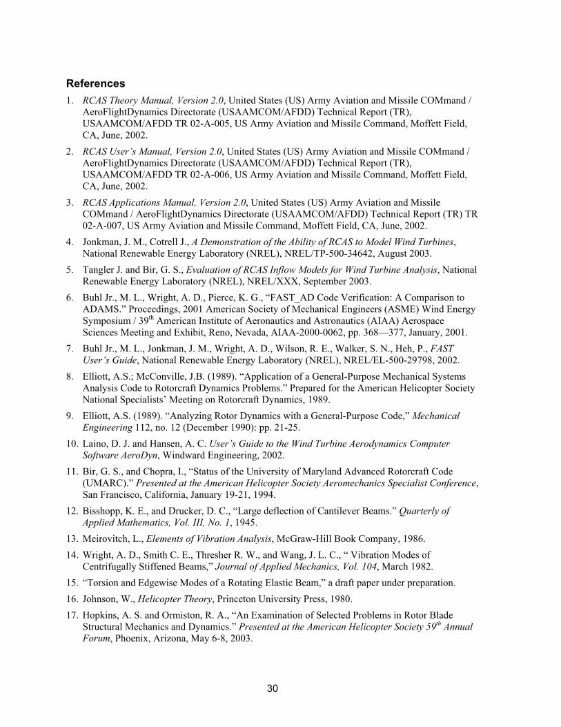
30

References 1. RCAS Theory Manual, Version 2.0, United States (US) Army Aviation and Missile COMmand /

AeroFlightDynamics Directorate (USAAMCOM/AFDD) Technical Report (TR), USAAMCOM/AFDD TR 02-A-005, US Army Aviation and Missile Command, Moffett Field, CA, June, 2002.

2. RCAS User’s Manual, Version 2.0, United States (US) Army Aviation and Missile COMmand / AeroFlightDynamics Directorate (USAAMCOM/AFDD) Technical Report (TR), USAAMCOM/AFDD TR 02-A-006, US Army Aviation and Missile Command, Moffett Field, CA, June, 2002.

3. RCAS Applications Manual, Version 2.0, United States (US) Army Aviation and Missile COMmand / AeroFlightDynamics Directorate (USAAMCOM/AFDD) Technical Report (TR) TR 02-A-007, US Army Aviation and Missile Command, Moffett Field, CA, June, 2002.

4. Jonkman, J. M., Cotrell J., A Demonstration of the Ability of RCAS to Model Wind Turbines, National Renewable Energy Laboratory (NREL), NREL/TP-500-34642, August 2003.

5. Tangler J. and Bir, G. S., Evaluation of RCAS Inflow Models for Wind Turbine Analysis, National Renewable Energy Laboratory (NREL), NREL/XXX, September 2003.

6. Buhl Jr., M. L., Wright, A. D., Pierce, K. G., “FAST_AD Code Verification: A Comparison to ADAMS.” Proceedings, 2001 American Society of Mechanical Engineers (ASME) Wind Energy Symposium / 39th American Institute of Aeronautics and Astronautics (AIAA) Aerospace Sciences Meeting and Exhibit, Reno, Nevada, AIAA-2000-0062, pp. 368—377, January, 2001.

7. Buhl Jr., M. L., Jonkman, J. M., Wright, A. D., Wilson, R. E., Walker, S. N., Heh, P., FAST User’s Guide, National Renewable Energy Laboratory (NREL), NREL/EL-500-29798, 2002.

8. Elliott, A.S.; McConville, J.B. (1989). “Application of a General-Purpose Mechanical Systems Analysis Code to Rotorcraft Dynamics Problems.” Prepared for the American Helicopter Society National Specialists’ Meeting on Rotorcraft Dynamics, 1989.

9. Elliott, A.S. (1989). “Analyzing Rotor Dynamics with a General-Purpose Code,” Mechanical Engineering 112, no. 12 (December 1990): pp. 21-25.

10. Laino, D. J. and Hansen, A. C. User’s Guide to the Wind Turbine Aerodynamics Computer Software AeroDyn, Windward Engineering, 2002.

11. Bir, G. S., and Chopra, I., “Status of the University of Maryland Advanced Rotorcraft Code (UMARC).” Presented at the American Helicopter Society Aeromechanics Specialist Conference, San Francisco, California, January 19-21, 1994.

12. Bisshopp, K. E., and Drucker, D. C., “Large deflection of Cantilever Beams.” Quarterly of Applied Mathematics, Vol. III, No. 1, 1945.

13. Meirovitch, L., Elements of Vibration Analysis, McGraw-Hill Book Company, 1986. 14. Wright, A. D., Smith C. E., Thresher R. W., and Wang, J. L. C., “ Vibration Modes of

Centrifugally Stiffened Beams,” Journal of Applied Mechanics, Vol. 104, March 1982. 15. “Torsion and Edgewise Modes of a Rotating Elastic Beam,” a draft paper under preparation. 16. Johnson, W., Helicopter Theory, Princeton University Press, 1980. 17. Hopkins, A. S. and Ormiston, R. A., “An Examination of Selected Problems in Rotor Blade

Structural Mechanics and Dynamics.” Presented at the American Helicopter Society 59th Annual Forum, Phoenix, Arizona, May 6-8, 2003.

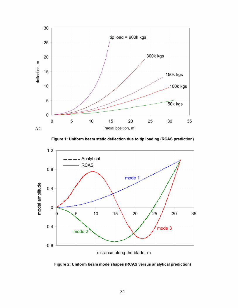
31

0

5

10

15

20

25

30

0 5 10 15 20 25 30 35radial position, m

defle

ctio

n, m

tip load = 900k kgs

100k kgs

300k kgs

50k kgs

150k kgs

-0.8

-0.4

0

0.4

0.8

1.2

0 5 10 15 20 25 30 35

distance along the blade, m

mod

al a

mpl

itude

mode 1

mode 2mode 3

AnalyticalRCAS

Figure 1: Uniform beam static deflection due to tip loading (RCAS prediction)

Figure 2: Uniform beam mode shapes (RCAS versus analytical prediction)

A2-

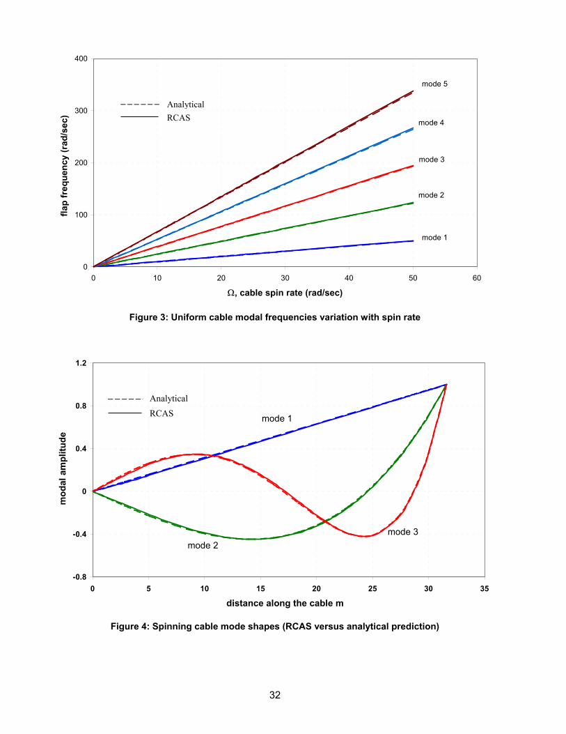
32

Figure 3: Uniform cable modal frequencies variation with spin rate

Figure 4: Spinning cable mode shapes (RCAS versus analytical prediction)

-0.8

-0.4

0

0.4

0.8

1.2

0 5 10 15 20 25 30 35

distance along the cable m

mod

al a

mpl

itude

mode 1

mode 2mode 3

AnalyticalRCAS

0

100

200

300

400

0 10 20 30 40 50 60

Ω, cable spin rate (rad/sec)

flap

freq

uenc

y (r

ad/s

ec)

mode 1

mode 5

mode 4

mode 2

mode 3

AnalyticalRCAS

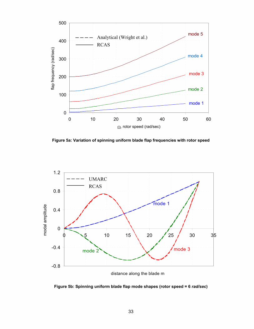
33

0

100

200

300

400

500

0 10 20 30 40 50 60

Ω, rotor speed (rad/sec)

flap

frequ

ency

(rad

/sec

)

mode 1

mode 5

mode 4

mode 2

mode 3

Figure 5a: Variation of spinning uniform blade flap frequencies with rotor speed

Figure 5b: Spinning uniform blade flap mode shapes (rotor speed = 6 rad/sec)

Analytical (Wright et al.)RCAS

UMARCRCAS

-0.8

-0.4

0

0.4

0.8

1.2

0 5 10 15 20 25 30 35

distance along the blade m

mod

al a

mpl

itude

mode 1

mode 2 mode 3

UMARCRCAS

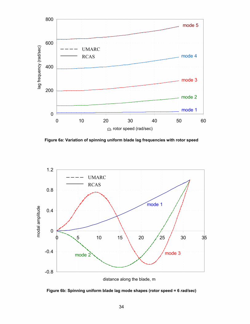
34

0

200

400

600

800

0 10 20 30 40 50 60

Ω, rotor speed (rad/sec)

lag

frequ

ency

(rad

/sec

)

mode 1

mode 5

mode 4

mode 2

mode 3

-0.8

-0.4

0

0.4

0.8

1.2

0 5 10 15 20 25 30 35

distance along the blade, m

mod

al a

mpl

itude

mode 1

mode 2 mode 3

Figure 6a: Variation of spinning uniform blade lag frequencies with rotor speed

Figure 6b: Spinning uniform blade lag mode shapes (rotor speed = 6 rad/sec)

UMARC RCAS

UMARCRCAS

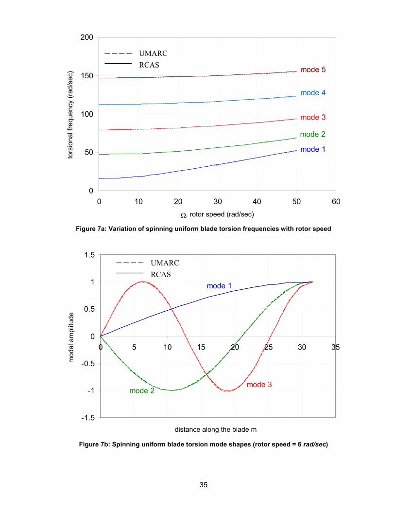
35

0

50

100

150

200

0 10 20 30 40 50 60

Ω, rotor speed (rad/sec)

tors

iona

l fre

quen

cy (r

ad/s

ec)

mode 1

mode 5

mode 4

mode 2

mode 3

-1.5

-1

-0.5

0

0.5

1

1.5

0 5 10 15 20 25 30 35

distance along the blade m

mod

al a

mpl

itude

mode 1

mode 2mode 3

Figure 7a: Variation of spinning uniform blade torsion frequencies with rotor speed

Figure 7b: Spinning uniform blade torsion mode shapes (rotor speed = 6 rad/sec)

UMARCRCAS

UMARCRCAS

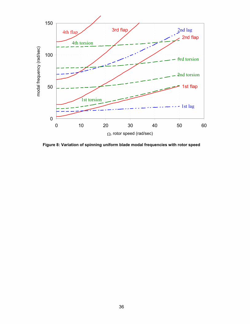
36

0

50

100

150

0 10 20 30 40 50 60

Ω, rotor speed (rad/sec)

mod

al fr

eque

ncy

(rad/

sec)

1st flap

2nd flap3rd flap

Figure 8: Variation of spinning uniform blade modal frequencies with rotor speed

1st lag

2nd lag

1st torsion

2nd torsion

3rd torsion

4th torsion

4th flap

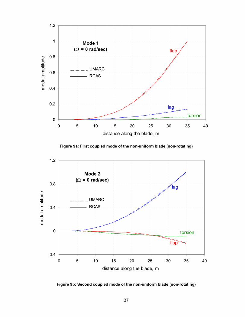
37

0

0.2

0.4

0.6

0.8

1

1.2

0 5 10 15 20 25 30 35 40

distance along the blade, m

mod

al a

mpl

itude

lag

torsion

flapMode 1

(Ω = 0 rad/sec)

UMARCRCAS

-0.4

0

0.4

0.8

1.2

0 5 10 15 20 25 30 35 40

distance along the blade, m

mod

al a

mpl

itude

lag

torsion

flap

Mode 2(Ω = 0 rad/sec)

UMARC

RCAS

Figure 9a: First coupled mode of the non-uniform blade (non-rotating)

Figure 9b: Second coupled mode of the non-uniform blade (non-rotating)

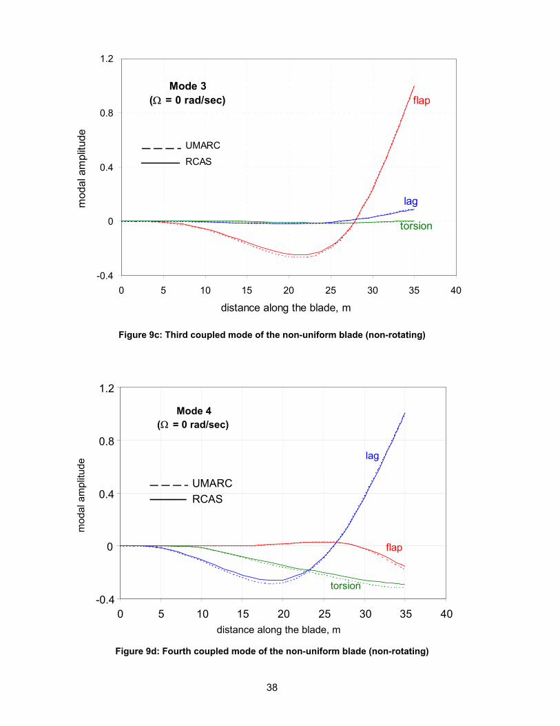
38

-0.4

0

0.4

0.8

1.2

0 5 10 15 20 25 30 35 40

distance along the blade, m

mod

al a

mpl

itude

lag

torsion

flapMode 3

(Ω = 0 rad/sec)

UMARC

RCAS

-0.4

0

0.4

0.8

1.2

0 5 10 15 20 25 30 35 40distance along the blade, m

mod

al a

mpl

itude

lag

torsion

flap

Mode 4 ( Ω = 0 rad/sec)

UMARCRCAS

Figure 9c: Third coupled mode of the non-uniform blade (non-rotating)

Figure 9d: Fourth coupled mode of the non-uniform blade (non-rotating)

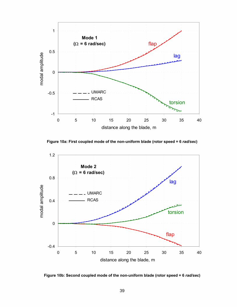
39

-1

-0.5

0

0.5

1

0 5 10 15 20 25 30 35 40

distance along the blade, m

mod

al a

mpl

itude lag

torsion

flapMode 1

(Ω = 6 rad/sec)

UMARC

RCAS

-0.4

0

0.4

0.8

1.2

0 5 10 15 20 25 30 35 40

distance along the blade, m

mod

al a

mpl

itude

lag

torsion

flap

Mode 2(Ω = 6 rad/sec)

UMARC

RCAS

Figure 10a: First coupled mode of the non-uniform blade (rotor speed = 6 rad/sec)

Figure 10b: Second coupled mode of the non-uniform blade (rotor speed = 6 rad/sec)

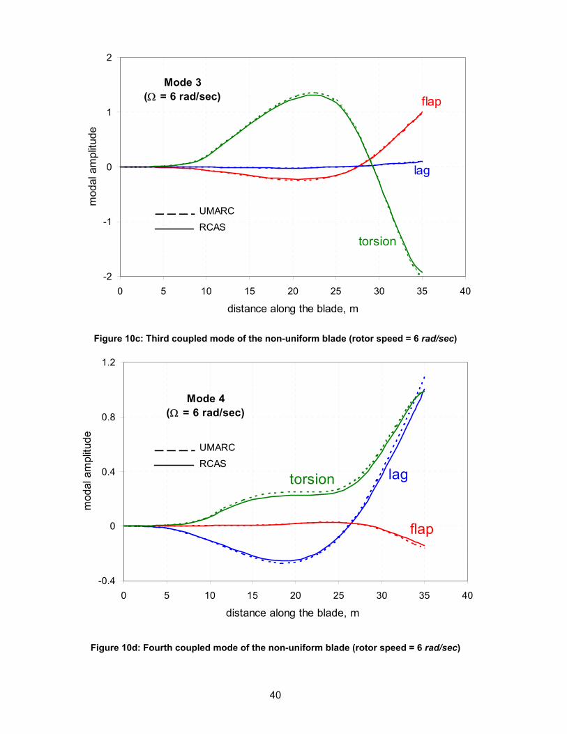
40

-2

-1

0

1

2

0 5 10 15 20 25 30 35 40

distance along the blade, m

mod

al a

mpl

itude

lag

torsion

flapMode 3

(Ω = 6 rad/sec)

UMARC

RCAS

-0.4

0

0.4

0.8

1.2

0 5 10 15 20 25 30 35 40

distance along the blade, m

mod

al a

mpl

itude

lagtorsion

flap

Mode 4(Ω = 6 rad/sec)

UMARC

RCAS

Figure 10c: Third coupled mode of the non-uniform blade (rotor speed = 6 rad/sec)

Figure 10d: Fourth coupled mode of the non-uniform blade (rotor speed = 6 rad/sec)

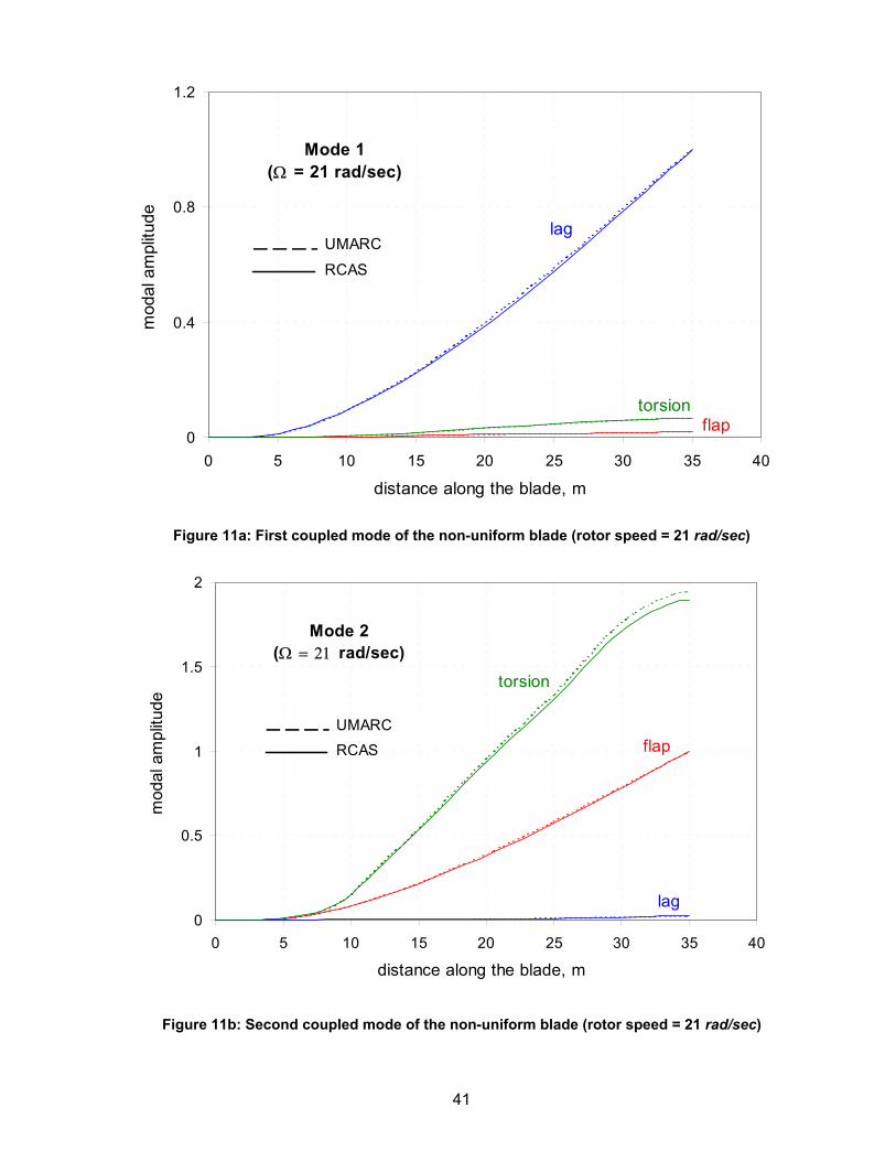
41

0

0.4

0.8

1.2

0 5 10 15 20 25 30 35 40

distance along the blade, m

mod

al a

mpl

itude lag

torsionflap

Mode 1(Ω = 21 rad/sec)

UMARC

RCAS

0

0.5

1

1.5

2

0 5 10 15 20 25 30 35 40

distance along the blade, m

mod

al a

mpl

itude

lag

torsion

flap

Mode 2(Ω = 21 rad/sec)

UMARCRCAS

Figure 11a: First coupled mode of the non-uniform blade (rotor speed = 21 rad/sec)

Figure 11b: Second coupled mode of the non-uniform blade (rotor speed = 21 rad/sec)

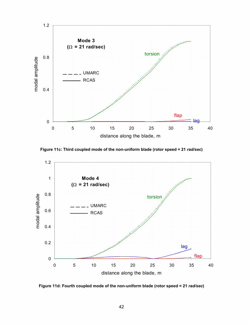
42

0

0.4

0.8

1.2

0 5 10 15 20 25 30 35 40

distance along the blade, m

mod

al a

mpl

itude

lag

torsion

flap

Mode 3(Ω = 21 rad/sec)

UMARC

RCAS

0

0.2

0.4

0.6

0.8

1

1.2

0 5 10 15 20 25 30 35 40

distance along the blade, m

mod

al a

mpl

itude

lag

torsion

flap

Mode 4(Ω = 21 rad/sec)

UMARC

RCAS

Figure 11c: Third coupled mode of the non-uniform blade (rotor speed = 21 rad/sec)

Figure 11d: Fourth coupled mode of the non-uniform blade (rotor speed = 21 rad/sec)

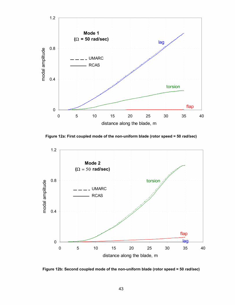
43

0

0.4

0.8

1.2

0 5 10 15 20 25 30 35 40

distance along the blade, m

mod

al a

mpl

itude

lag

torsion

flap

Mode 1(Ω = 50 rad/sec)

UMARC

RCAS

0

0.4

0.8

1.2

0 5 10 15 20 25 30 35 40

distance along the blade, m

mod

al a

mpl

itude

lag

torsion

flap

Mode 2(Ω = 50 rad/sec)

UMARC

RCAS

Figure 12a: First coupled mode of the non-uniform blade (rotor speed = 50 rad/sec)

Figure 12b: Second coupled mode of the non-uniform blade (rotor speed = 50 rad/sec)

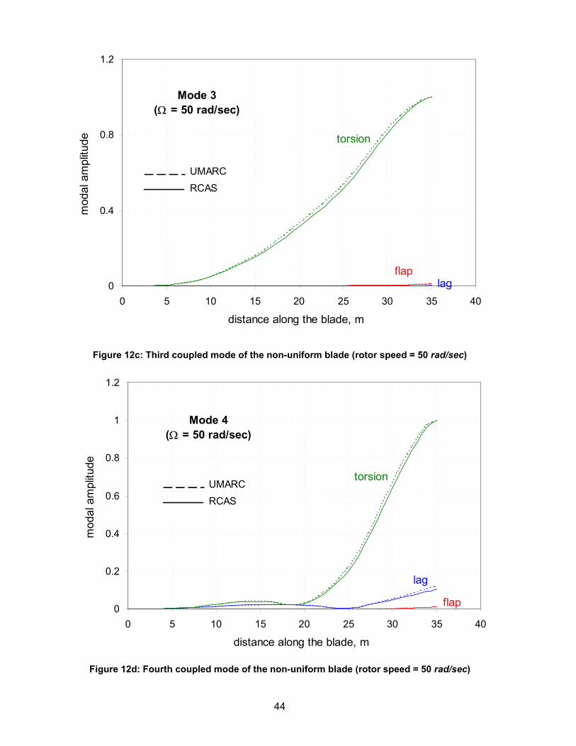
44

0

0.4

0.8

1.2

0 5 10 15 20 25 30 35 40

distance along the blade, m

mod

al a

mpl

itude

lag

torsion

flap

Mode 3(Ω = 50 rad/sec)

UMARC

RCAS

0

0.2

0.4

0.6

0.8

1

1.2

0 5 10 15 20 25 30 35 40

distance along the blade, m

mod

al a

mpl

itude

lag

torsion

flap

Mode 4(Ω = 50 rad/sec)

UMARC

RCAS

Figure 12c: Third coupled mode of the non-uniform blade (rotor speed = 50 rad/sec)

Figure 12d: Fourth coupled mode of the non-uniform blade (rotor speed = 50 rad/sec)

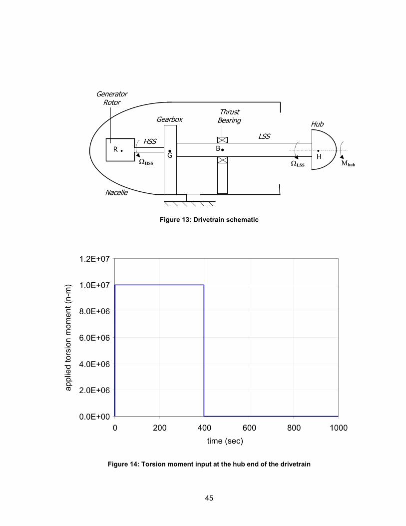
45

0.0E+00

2.0E+06

4.0E+06

6.0E+06

8.0E+06

1.0E+07

1.2E+07

0 200 400 600 800 1000 time (sec)

appl

ied

tors

ion

mom

ent (

n-m

)

Figure 13: Drivetrain schematic

Figure 14: Torsion moment input at the hub end of the drivetrain

Μhub

Nacelle

Generator Rotor

HSS

Hub

ThrustBearing

. . . . LSS

Gearbox

G B

H R

ΩHSS ΩLSS

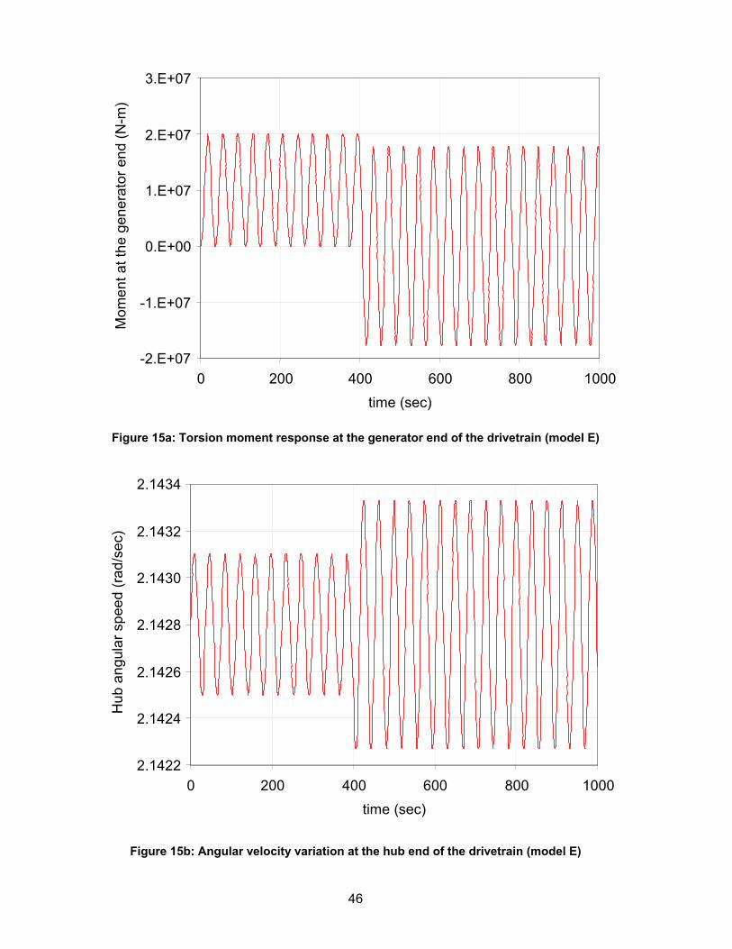
46

-2.E+07

-1.E+07

0.E+00

1.E+07

2.E+07

3.E+07

0 200 400 600 800 1000time (sec)

Mom

ent a

t the

gen

erat

or e

nd (N

-m)

2.1422

2.1424

2.1426

2.1428

2.1430

2.1432

2.1434

0 200 400 600 800 1000time (sec)

Hub

ang

ular

spe

ed (r

ad/s

ec)

Figure 15a: Torsion moment response at the generator end of the drivetrain (model E)

Figure 15b: Angular velocity variation at the hub end of the drivetrain (model E)

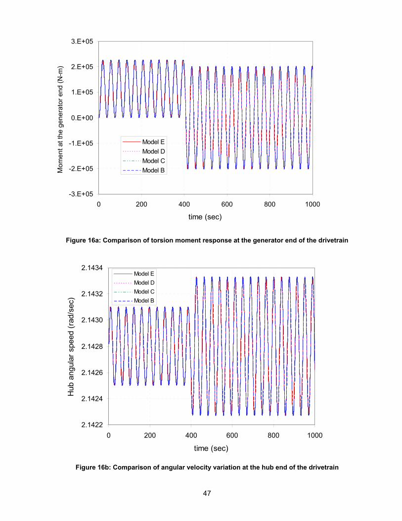
47

-3.E+05

-2.E+05

-1.E+05

0.E+00

1.E+05

2.E+05

3.E+05

0 200 400 600 800 1000

time (sec)

Mom

ent a

t the

gen

erat

or e

nd (N

-m)

Model EModel DModel CModel B

2.1422

2.1424

2.1426

2.1428

2.1430

2.1432

2.1434

0 200 400 600 800 1000

time (sec)

Hub

ang

ular

spe

ed (r

ad/s

ec)

Model EModel DModel CModel B

Figure 16a: Comparison of torsion moment response at the generator end of the drivetrain

Figure 16b: Comparison of angular velocity variation at the hub end of the drivetrain

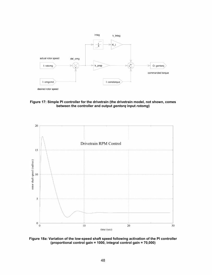
48

Figure 17: Simple PI controller for the drivetrain (the drivetrain model, not shown, comes between the controller and output gentorq input rotomg)

Figure 18a: Variation of the low-speed shaft speed following activation of the PI controller (proportional control gain = 1000, integral control gain = 70,000)

Drivetrain RPM Control

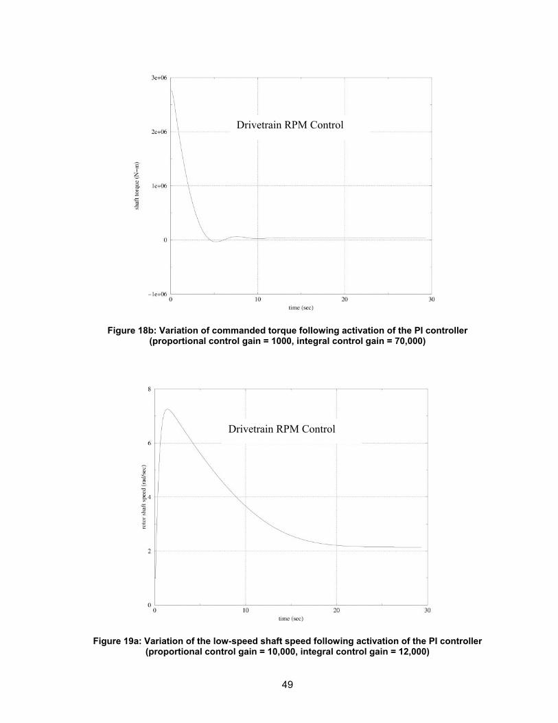
49

Figure 18b: Variation of commanded torque following activation of the PI controller (proportional control gain = 1000, integral control gain = 70,000)

Figure 19a: Variation of the low-speed shaft speed following activation of the PI controller (proportional control gain = 10,000, integral control gain = 12,000)

Drivetrain RPM Control

Drivetrain RPM Control

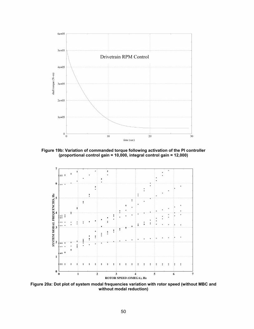
50

Figure 19b: Variation of commanded torque following activation of the PI controller (proportional control gain = 10,000, integral control gain = 12,000)

Figure 20a: Dot plot of system modal frequencies variation with rotor speed (without MBC and without modal reduction)

Drivetrain RPM Control

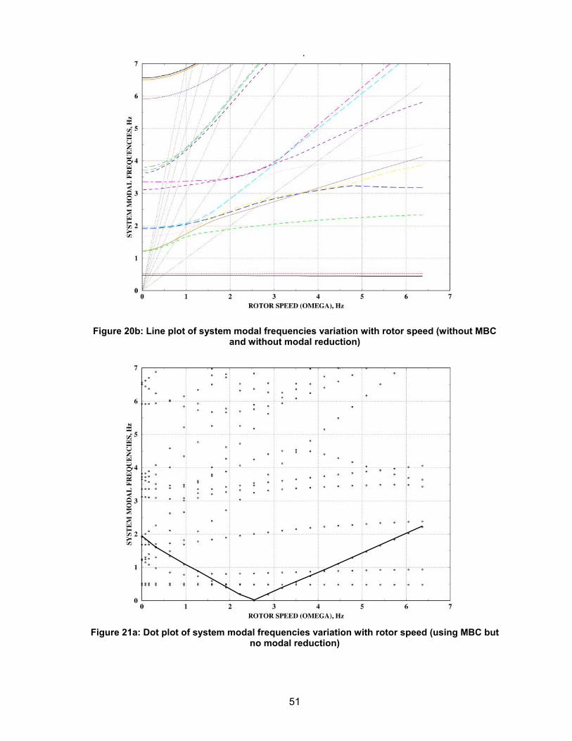
51

Figure 20b: Line plot of system modal frequencies variation with rotor speed (without MBC and without modal reduction)

Figure 21a: Dot plot of system modal frequencies variation with rotor speed (using MBC but no modal reduction)

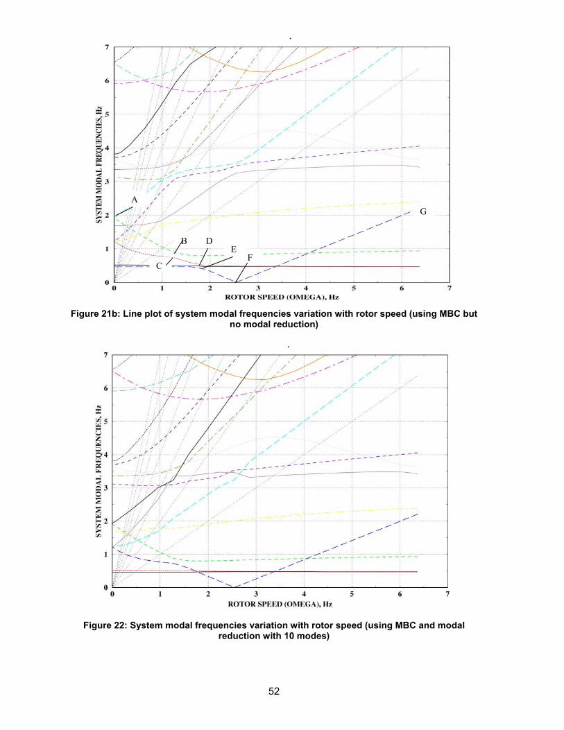
52

Figure 21b: Line plot of system modal frequencies variation with rotor speed (using MBC but no modal reduction)

Figure 22: System modal frequencies variation with rotor speed (using MBC and modal reduction with 10 modes)

A

B

C

D E

F

G

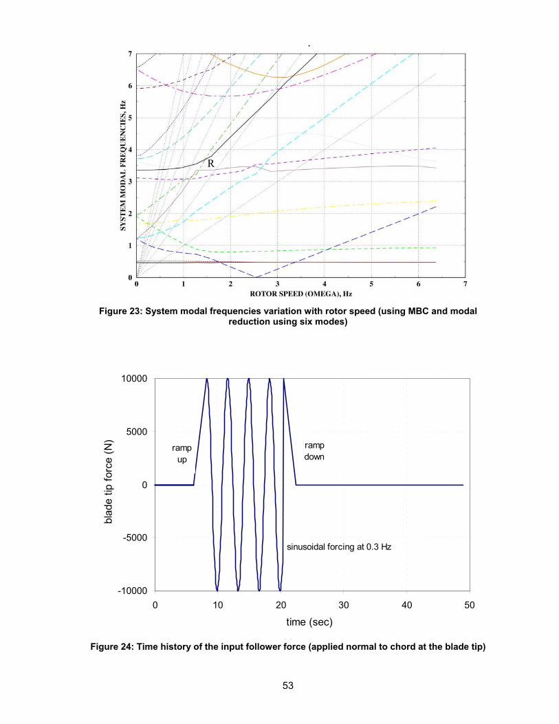
53

Figure 23: System modal frequencies variation with rotor speed (using MBC and modal reduction using six modes)

Fi Figure 24: Time history of the input follower force (applied normal to chord at the blade tip)

R

-10000

-5000

0

5000

10000

0 10 20 30 40 50

time (sec)

blad

e tip

forc

e (N

)

rampup

sinusoidal forcing at 0.3 Hz

rampdown

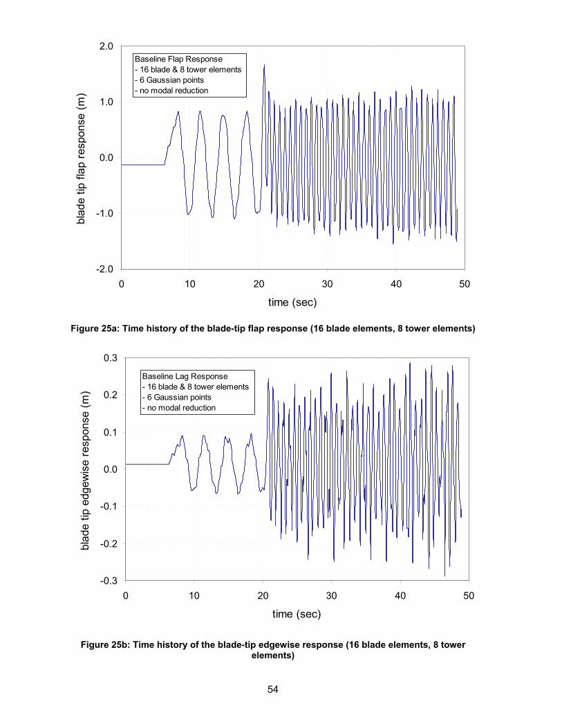
54

-2.0

-1.0

0.0

1.0

2.0

0 10 20 30 40 50

time (sec)

blad

e tip

flap

resp

onse

(m)

Baseline Flap Response- 16 blade & 8 tower elements- 6 Gaussian points- no modal reduction

-0.3

-0.2

-0.1

0.0

0.1

0.2

0.3

0 10 20 30 40 50

time (sec)

blad

e tip

edg

ewis

e re

spon

se (m

)

Baseline Lag Response- 16 blade & 8 tower elements- 6 Gaussian points- no modal reduction

Figure 25a: Time history of the blade-tip flap response (16 blade elements, 8 tower elements)

Figure 25b: Time history of the blade-tip edgewise response (16 blade elements, 8 tower elements)

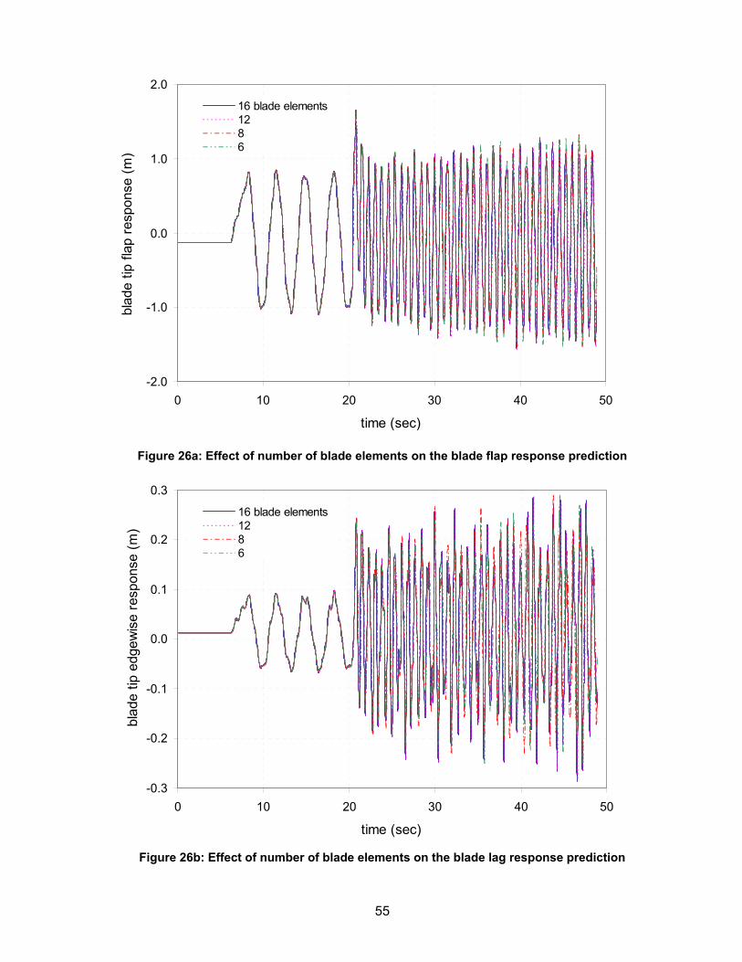
55

-2.0

-1.0

0.0

1.0

2.0

0 10 20 30 40 50

time (sec)

blad

e tip

flap

resp

onse

(m)

16 blade elements1286

-0.3

-0.2

-0.1

0.0

0.1

0.2

0.3

0 10 20 30 40 50

time (sec)

blad

e tip

edg

ewis

e re

spon

se (m

)

16 blade elements1286

Figure 26a: Effect of number of blade elements on the blade flap response prediction

Figure 26b: Effect of number of blade elements on the blade lag response prediction

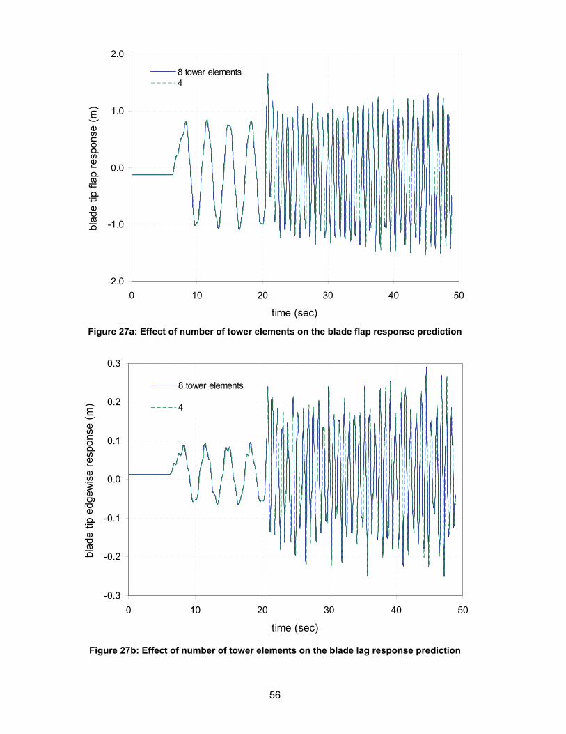
56

-2.0

-1.0

0.0

1.0

2.0

0 10 20 30 40 50

time (sec)

blad

e tip

flap

resp

onse

(m)

8 tower elements4

-0.3

-0.2

-0.1

0.0

0.1

0.2

0.3

0 10 20 30 40 50

time (sec)

blad

e tip

edg

ewis

e re

spon

se (m

)

8 tower elements

4

Figure 27a: Effect of number of tower elements on the blade flap response prediction

Figure 27b: Effect of number of tower elements on the blade lag response prediction

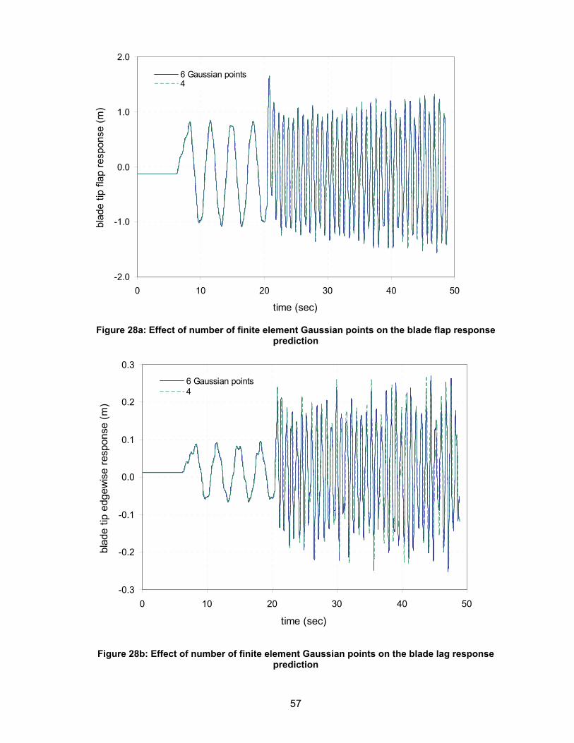
57

-2.0

-1.0

0.0

1.0

2.0

0 10 20 30 40 50

time (sec)

blad

e tip

flap

resp

onse

(m)

6 Gaussian points4

-0.3

-0.2

-0.1

0.0

0.1

0.2

0.3

0 10 20 30 40 50

time (sec)

blad

e tip

edg

ewis

e re

spon

se (m

)

6 Gaussian points4

Figure 28a: Effect of number of finite element Gaussian points on the blade flap response

prediction

Figure 28b: Effect of number of finite element Gaussian points on the blade lag response prediction

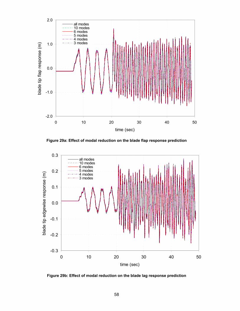
58

-0.3

-0.2

-0.1

0.0

0.1

0.2

0.3

0 10 20 30 40 50

time (sec)

blad

e tip

edg

ewis

e re

spon

se (m

)

all modes10 modes6 modes5 modes4 modes3 modes

-2.0

-1.0

0.0

1.0

2.0

0 10 20 30 40 50

time (sec)

blad

e tip

flap

resp

onse

(m)

all modes10 modes6 modes5 modes4 modes3 modes

Figure 29a: Effect of modal reduction on the blade flap response prediction

Figure 29b: Effect of modal reduction on the blade lag response prediction

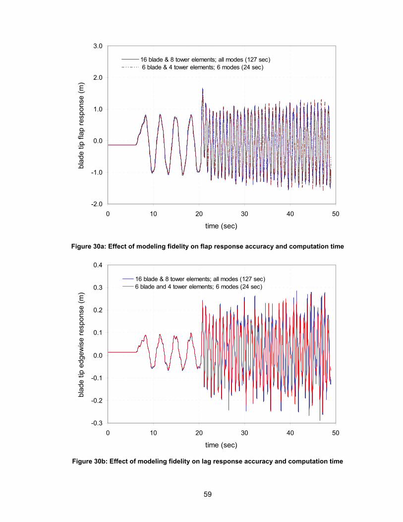
59

-2.0

-1.0

0.0

1.0

2.0

3.0

0 10 20 30 40 50

time (sec)

blad

e tip

flap

resp

onse

(m)

16 blade & 8 tower elements; all modes (127 sec) 6 blade & 4 tower elements; 6 modes (24 sec)

-0.3

-0.2

-0.1

0.0

0.1

0.2

0.3

0.4

0 10 20 30 40 50

time (sec)

blad

e tip

edg

ewis

e re

spon

se (m

)

16 blade & 8 tower elements; all modes (127 sec)6 blade and 4 tower elements; 6 modes (24 sec)

Figure 30a: Effect of modeling fidelity on flap response accuracy and computation time

Figure 30b: Effect of modeling fidelity on lag response accuracy and computation time

60

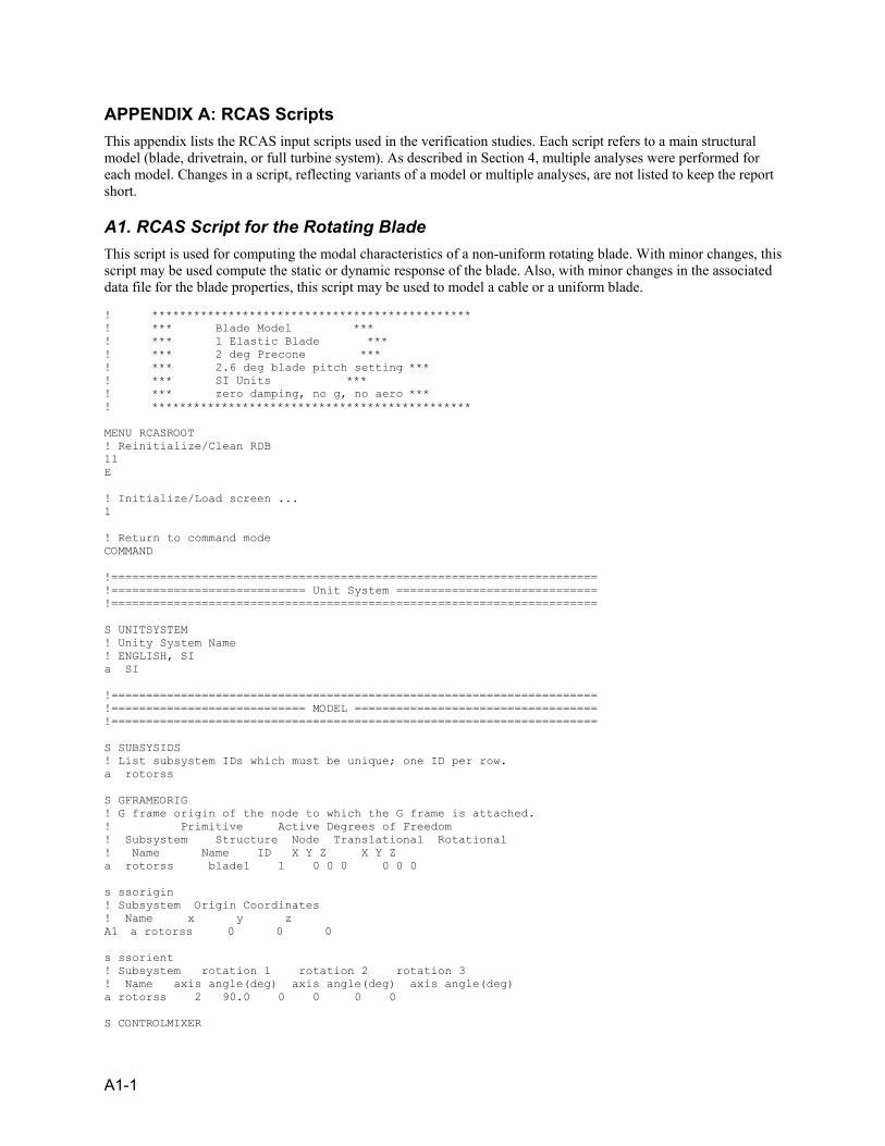
A1-1

APPENDIX A: RCAS Scripts This appendix lists the RCAS input scripts used in the verification studies. Each script refers to a main structural model (blade, drivetrain, or full turbine system). As described in Section 4, multiple analyses were performed for each model. Changes in a script, reflecting variants of a model or multiple analyses, are not listed to keep the report short.

A1. RCAS Script for the Rotating Blade This script is used for computing the modal characteristics of a non-uniform rotating blade. With minor changes, this script may be used compute the static or dynamic response of the blade. Also, with minor changes in the associated data file for the blade properties, this script may be used to model a cable or a uniform blade. ! ********************************************** ! *** Blade Model *** ! *** 1 Elastic Blade *** ! *** 2 deg Precone *** ! *** 2.6 deg blade pitch setting *** ! *** SI Units *** ! *** zero damping, no g, no aero *** ! ********************************************** MENU RCASROOT ! Reinitialize/Clean RDB 11 E ! Initialize/Load screen ... 1 ! Return to command mode COMMAND !====================================================================== !============================ Unit System ============================= !====================================================================== S UNITSYSTEM ! Unity System Name ! ENGLISH, SI a SI !====================================================================== !============================ MODEL =================================== !====================================================================== S SUBSYSIDS ! List subsystem IDs which must be unique; one ID per row. a rotorss S GFRAMEORIG ! G frame origin of the node to which the G frame is attached. ! Primitive Active Degrees of Freedom ! Subsystem Structure Node Translational Rotational ! Name Name ID X Y Z X Y Z a rotorss blade1 1 0 0 0 0 0 0 s ssorigin ! Subsystem Origin Coordinates ! Name x y z A1 a rotorss 0 0 0 s ssorient ! Subsystem rotation 1 rotation 2 rotation 3 ! Name axis angle(deg) axis angle(deg) axis angle(deg) a rotorss 2 90.0 0 0 0 0 S CONTROLMIXER

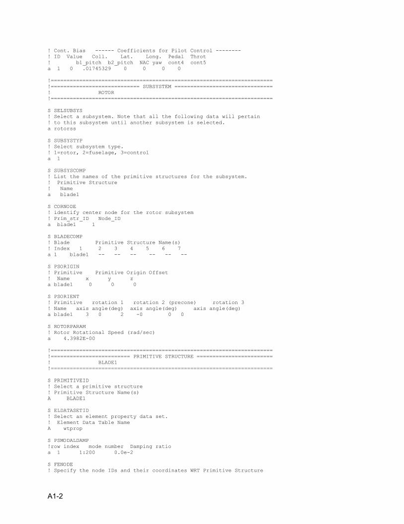
A1-2

! Cont. Bias ------ Coefficients for Pilot Control -------- ! ID Value Coll. Lat. Long. Pedal Throt ! b1_pitch b2_pitch NAC yaw cont4 cont5 a 1 0 .01745329 0 0 0 0 !====================================================================== !============================ SUBSYSTEM =============================== ! ROTOR !====================================================================== S SELSUBSYS ! Select a subsystem. Note that all the following data will pertain ! to this subsystem until another subsystem is selected. a rotorss S SUBSYSTYP ! Select subsystem type. ! 1=rotor, 2=fuselage, 3=control a 1 S SUBSYSCOMP ! List the names of the primitive structures for the subsystem. ! Primitive Structure ! Name a blade1 S CORNODE ! identify center node for the rotor subsystem ! Prim_str_ID Node_ID a blade1 1 S BLADECOMP ! Blade Primitive Structure Name(s) ! Index 1 2 3 4 5 6 7 a 1 blade1 -- -- -- -- -- -- S PSORIGIN ! Primitive Primitive Origin Offset ! Name x y z a blade1 0 0 0 S PSORIENT ! Primitive rotation 1 rotation 2 (precone) rotation 3 ! Name axis angle(deg) axis angle(deg) axis angle(deg) a blade1 3 0 2 -0 0 0 S ROTORPARAM ! Rotor Rotational Speed (rad/sec) a 4.3982E-00 !====================================================================== !========================= PRIMITIVE STRUCTURE ======================== ! BLADE1 !====================================================================== S PRIMITIVEID ! Select a primitive structure ! Primitive Structure Name(s) A BLADE1 S ELDATASETID ! Select an element property data set. ! Element Data Table Name A wtprop S PSMODALDAMP !row index mode number Damping ratio a 1 1:200 0.0e-2 S FENODE ! Specify the node IDs and their coordinates WRT Primitive Structure

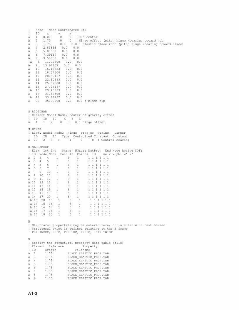
A1-3

! Node Node Coordinates (m) ! ID x y z A 1 0.00 0 0 ! Hub center A 2 1.75 0 0 ! Hinge offset (pitch hinge /bearing toward hub) A 3 1.75 0.0 0.0 ! Elastic blade root (pitch hinge /bearing toward blade) A 4 2.85833 0.0 0.0 A 5 5.07500 0.0 0.0 A 6 7.29167 0.0 0.0 A 7 9.50833 0.0 0.0 !A 8 11.72500 0.0 0.0 A 9 13.94167 0.0 0.0 A 10 16.15833 0.0 0.0 A 11 18.37500 0.0 0.0 A 12 20.59167 0.0 0.0 A 13 22.80833 0.0 0.0 A 14 25.02500 0.0 0.0 A 15 27.24167 0.0 0.0 !A 16 29.45833 0.0 0.0 A 17 31.67500 0.0 0.0 !A 18 33.89167 0.0 0.0 A 20 35.00000 0.0 0.0 ! blade tip S RIGIDBAR ! Element Node1 Node2 Center of gravity offset ! ID ID ID X Y Z A 1 1 2 0 0 0 ! Hinge offset S HINGE ! Elem. Node1 Node2 Hinge Free or Spring Damper ! ID ID ID Type Controlled Constant Constant A 20 2 3 P 1 0 0 ! Control bearing S NLBEAMDEF ! Elem 1st 2nd Shape NGauss MatProp End Node Active DOFs ! ID Node Node Func ID Points ID ue v w phi w' v' A 2 3 4 1 6 1 1 1 1 1 1 1 A 3 4 5 1 6 1 1 1 1 1 1 1 A 4 5 6 1 6 1 1 1 1 1 1 1 A 5 6 7 1 6 1 1 1 1 1 1 1 A 7 9 10 1 6 1 1 1 1 1 1 1 A 8 10 11 1 6 1 1 1 1 1 1 1 A 9 11 12 1 6 1 1 1 1 1 1 1 A 10 12 13 1 6 1 1 1 1 1 1 1 A 11 13 14 1 6 1 1 1 1 1 1 1 A 12 14 15 1 6 1 1 1 1 1 1 1 A 13 15 17 1 6 1 1 1 1 1 1 1 A 14 17 20 1 6 1 1 1 1 1 1 1 !A 15 20 15 1 6 1 1 1 1 1 1 1 !A 14 15 16 1 6 1 1 1 1 1 1 1 !A 15 16 17 1 6 1 1 1 1 1 1 1 !A 16 17 18 1 6 1 1 1 1 1 1 1 !A 17 18 20 1 6 1 1 1 1 1 1 1 N ! Structural properties may be entered here, or in a table in next screen ! Structural twist is defined relative to the E frame ! PRP-INDEX, ELID, PRP-LOC, PRPID, STR-TWIST N ! Specify the structural property data table (file) ! Element Refernce Property ! ID origin Filename A 2 1.75 BLADE_ELASTIC_PROP.TAB A 3 1.75 BLADE_ELASTIC_PROP.TAB A 4 1.75 BLADE_ELASTIC_PROP.TAB A 5 1.75 BLADE_ELASTIC_PROP.TAB A 6 1.75 BLADE_ELASTIC_PROP.TAB A 7 1.75 BLADE_ELASTIC_PROP.TAB A 8 1.75 BLADE_ELASTIC_PROP.TAB A 9 1.75 BLADE_ELASTIC_PROP.TAB

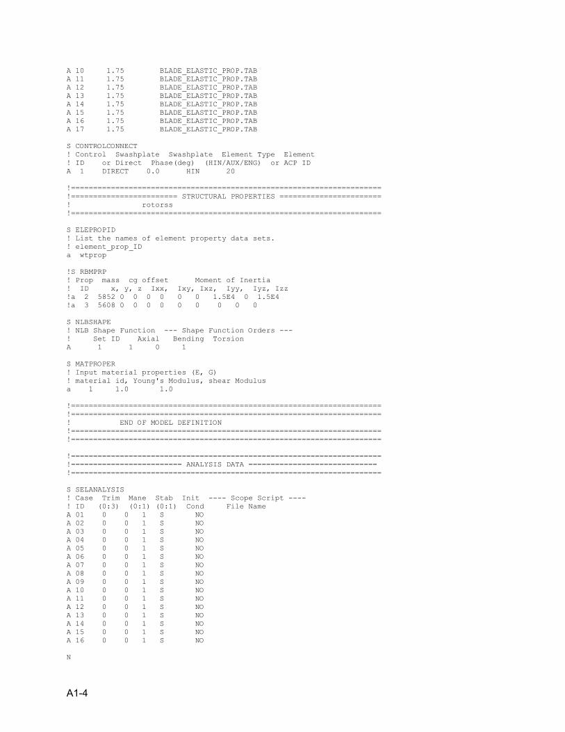
A1-4

A 10 1.75 BLADE_ELASTIC_PROP.TAB A 11 1.75 BLADE_ELASTIC_PROP.TAB A 12 1.75 BLADE_ELASTIC_PROP.TAB A 13 1.75 BLADE_ELASTIC_PROP.TAB A 14 1.75 BLADE_ELASTIC_PROP.TAB A 15 1.75 BLADE_ELASTIC_PROP.TAB A 16 1.75 BLADE_ELASTIC_PROP.TAB A 17 1.75 BLADE_ELASTIC_PROP.TAB S CONTROLCONNECT ! Control Swashplate Swashplate Element Type Element ! ID or Direct Phase(deg) (HIN/AUX/ENG) or ACP ID A 1 DIRECT 0.0 HIN 20 !====================================================================== !======================== STRUCTURAL PROPERTIES ======================= ! rotorss !====================================================================== S ELEPROPID ! List the names of element property data sets. ! element_prop_ID a wtprop !S RBMPRP ! Prop mass cg offset Moment of Inertia ! ID x, y, z Ixx, Ixy, Ixz, Iyy, Iyz, Izz !a 2 5852 0 0 0 0 0 0 1.5E4 0 1.5E4 !a 3 5608 0 0 0 0 0 0 0 0 0 S NLBSHAPE ! NLB Shape Function --- Shape Function Orders --- ! Set ID Axial Bending Torsion A 1 1 0 1 S MATPROPER ! Input material properties (E, G) ! material id, Young's Modulus, shear Modulus a 1 1.0 1.0 !====================================================================== !====================================================================== ! END OF MODEL DEFINITION !====================================================================== !====================================================================== !====================================================================== !========================= ANALYSIS DATA ============================= !====================================================================== S SELANALYSIS ! Case Trim Mane Stab Init ---- Scope Script ---- ! ID (0:3) (0:1) (0:1) Cond File Name A 01 0 0 1 S NO A 02 0 0 1 S NO A 03 0 0 1 S NO A 04 0 0 1 S NO A 05 0 0 1 S NO A 06 0 0 1 S NO A 07 0 0 1 S NO A 08 0 0 1 S NO A 09 0 0 1 S NO A 10 0 0 1 S NO A 11 0 0 1 S NO A 12 0 0 1 S NO A 13 0 0 1 S NO A 14 0 0 1 S NO A 15 0 0 1 S NO A 16 0 0 1 S NO N

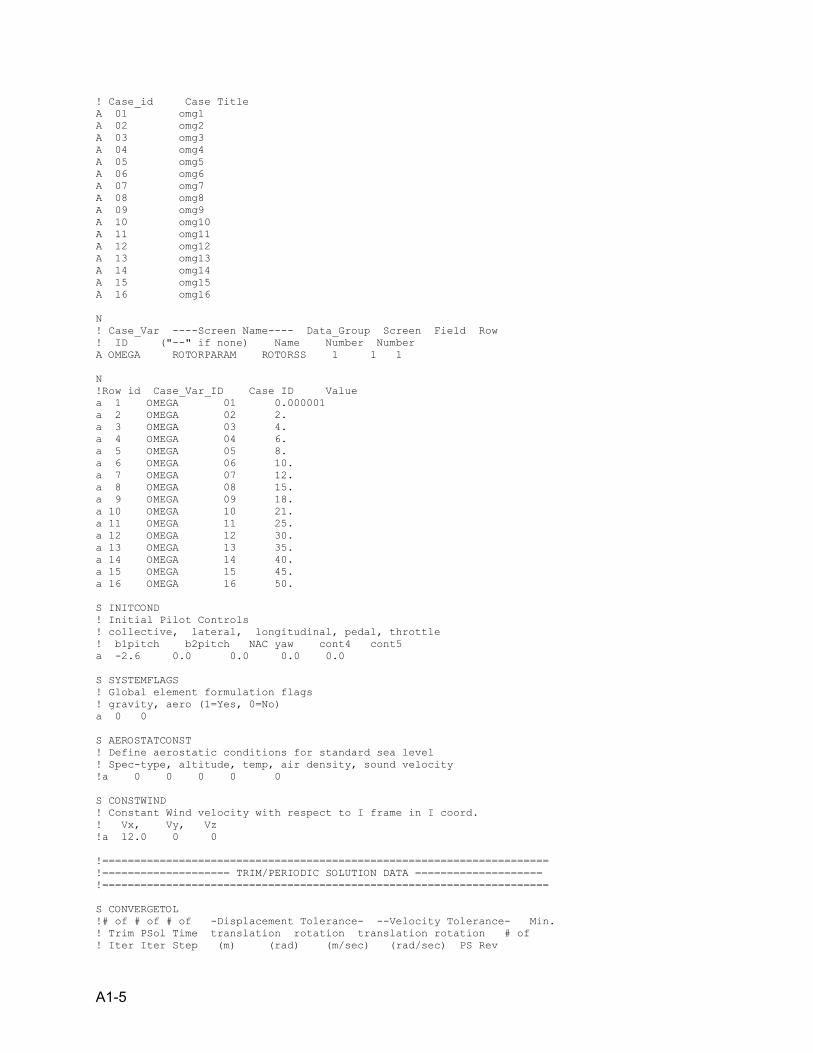
A1-5

! Case_id Case Title A 01 omg1 A 02 omg2 A 03 omg3 A 04 omg4 A 05 omg5 A 06 omg6 A 07 omg7 A 08 omg8 A 09 omg9 A 10 omg10 A 11 omg11 A 12 omg12 A 13 omg13 A 14 omg14 A 15 omg15 A 16 omg16 N ! Case_Var ----Screen Name---- Data_Group Screen Field Row ! ID ("--" if none) Name Number Number A OMEGA ROTORPARAM ROTORSS 1 1 1 N !Row id Case_Var_ID Case ID Value a 1 OMEGA 01 0.000001 a 2 OMEGA 02 2. a 3 OMEGA 03 4. a 4 OMEGA 04 6. a 5 OMEGA 05 8. a 6 OMEGA 06 10. a 7 OMEGA 07 12. a 8 OMEGA 08 15. a 9 OMEGA 09 18. a 10 OMEGA 10 21. a 11 OMEGA 11 25. a 12 OMEGA 12 30. a 13 OMEGA 13 35. a 14 OMEGA 14 40. a 15 OMEGA 15 45. a 16 OMEGA 16 50. S INITCOND ! Initial Pilot Controls ! collective, lateral, longitudinal, pedal, throttle ! b1pitch b2pitch NAC yaw cont4 cont5 a -2.6 0.0 0.0 0.0 0.0 S SYSTEMFLAGS ! Global element formulation flags ! gravity, aero (1=Yes, 0=No) a 0 0 S AEROSTATCONST ! Define aerostatic conditions for standard sea level ! Spec-type, altitude, temp, air density, sound velocity !a 0 0 0 0 0 S CONSTWIND ! Constant Wind velocity with respect to I frame in I coord. ! Vx, Vy, Vz !a 12.0 0 0 !====================================================================== !==================== TRIM/PERIODIC SOLUTION DATA ==================== !====================================================================== S CONVERGETOL !# of # of # of -Displacement Tolerance- --Velocity Tolerance- Min. ! Trim PSol Time translation rotation translation rotation # of ! Iter Iter Step (m) (rad) (m/sec) (rad/sec) PS Rev

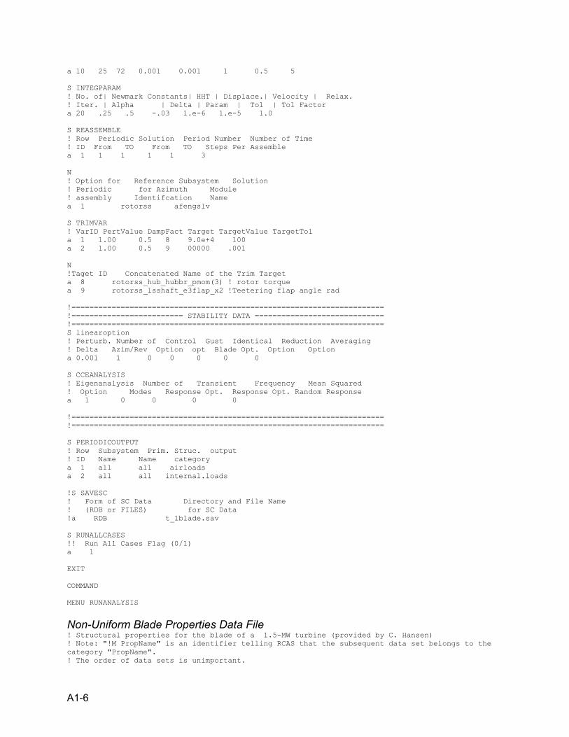
A1-6

a 10 25 72 0.001 0.001 1 0.5 5 S INTEGPARAM ! No. of| Newmark Constants| HHT | Displace.| Velocity | Relax. ! Iter. | Alpha | Delta | Param | Tol | Tol Factor a 20 .25 .5 -.03 1.e-6 1.e-5 1.0 S REASSEMBLE ! Row Periodic Solution Period Number Number of Time ! ID From TO From TO Steps Per Assemble a 1 1 1 1 1 3 N ! Option for Reference Subsystem Solution ! Periodic for Azimuth Module ! assembly Identifcation Name a 1 rotorss afengslv S TRIMVAR ! VarID PertValue DampFact Target TargetValue TargetTol a 1 1.00 0.5 8 9.0e+4 100 a 2 1.00 0.5 9 00000 .001 N !Taget ID Concatenated Name of the Trim Target a 8 rotorss_hub_hubbr_pmom(3) ! rotor torque a 9 rotorss_lsshaft_e3flap_x2 !Teetering flap angle rad !====================================================================== !========================= STABILITY DATA ============================= !====================================================================== S linearoption ! Perturb. Number of Control Gust Identical Reduction Averaging ! Delta Azim/Rev Option opt Blade Opt. Option Option a 0.001 1 0 0 0 0 0 S CCEANALYSIS ! Eigenanalysis Number of Transient Frequency Mean Squared ! Option Modes Response Opt. Response Opt. Random Response a 1 0 0 0 0 !====================================================================== !====================================================================== S PERIODICOUTPUT ! Row Subsystem Prim. Struc. output ! ID Name Name category a 1 all all airloads a 2 all all internal.loads !S SAVESC ! Form of SC Data Directory and File Name ! (RDB or FILES) for SC Data !a RDB t_1blade.sav S RUNALLCASES !! Run All Cases Flag (0/1) a 1 EXIT COMMAND MENU RUNANALYSIS

Non-Uniform Blade Properties Data File ! Structural properties for the blade of a 1.5-MW turbine (provided by C. Hansen) ! Note: "!M PropName" is an identifier telling RCAS that the subsequent data set belongs to the category "PropName". ! The order of data sets is unimportant.

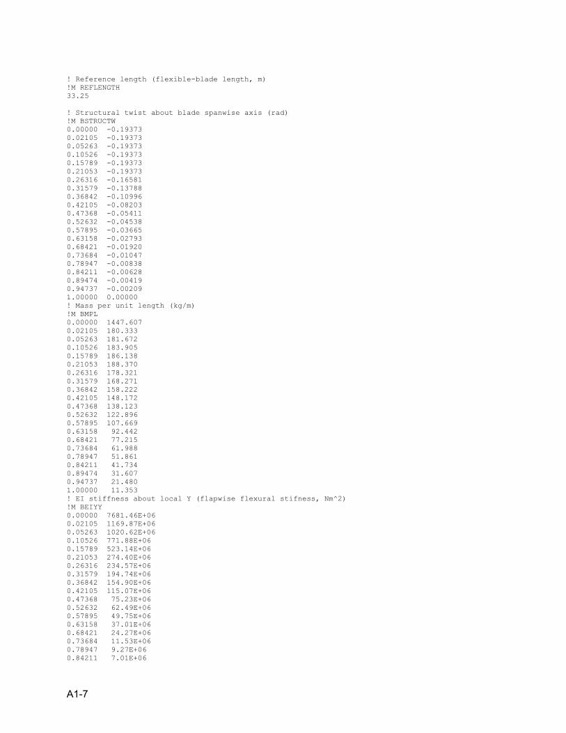
A1-7

! Reference length (flexible-blade length, m) !M REFLENGTH 33.25 ! Structural twist about blade spanwise axis (rad) !M BSTRUCTW 0.00000 -0.19373 0.02105 -0.19373 0.05263 -0.19373 0.10526 -0.19373 0.15789 -0.19373 0.21053 -0.19373 0.26316 -0.16581 0.31579 -0.13788 0.36842 -0.10996 0.42105 -0.08203 0.47368 -0.05411 0.52632 -0.04538 0.57895 -0.03665 0.63158 -0.02793 0.68421 -0.01920 0.73684 -0.01047 0.78947 -0.00838 0.84211 -0.00628 0.89474 -0.00419 0.94737 -0.00209 1.00000 0.00000 ! Mass per unit length (kg/m) !M BMPL 0.00000 1447.607 0.02105 180.333 0.05263 181.672 0.10526 183.905 0.15789 186.138 0.21053 188.370 0.26316 178.321 0.31579 168.271 0.36842 158.222 0.42105 148.172 0.47368 138.123 0.52632 122.896 0.57895 107.669 0.63158 92.442 0.68421 77.215 0.73684 61.988 0.78947 51.861 0.84211 41.734 0.89474 31.607 0.94737 21.480 1.00000 11.353 ! EI stiffness about local Y (flapwise flexural stifness, Nm^2) !M BEIYY 0.00000 7681.46E+06 0.02105 1169.87E+06 0.05263 1020.62E+06 0.10526 771.88E+06 0.15789 523.14E+06 0.21053 274.40E+06 0.26316 234.57E+06 0.31579 194.74E+06 0.36842 154.90E+06 0.42105 115.07E+06 0.47368 75.23E+06 0.52632 62.49E+06 0.57895 49.75E+06 0.63158 37.01E+06 0.68421 24.27E+06 0.73684 11.53E+06 0.78947 9.27E+06 0.84211 7.01E+06

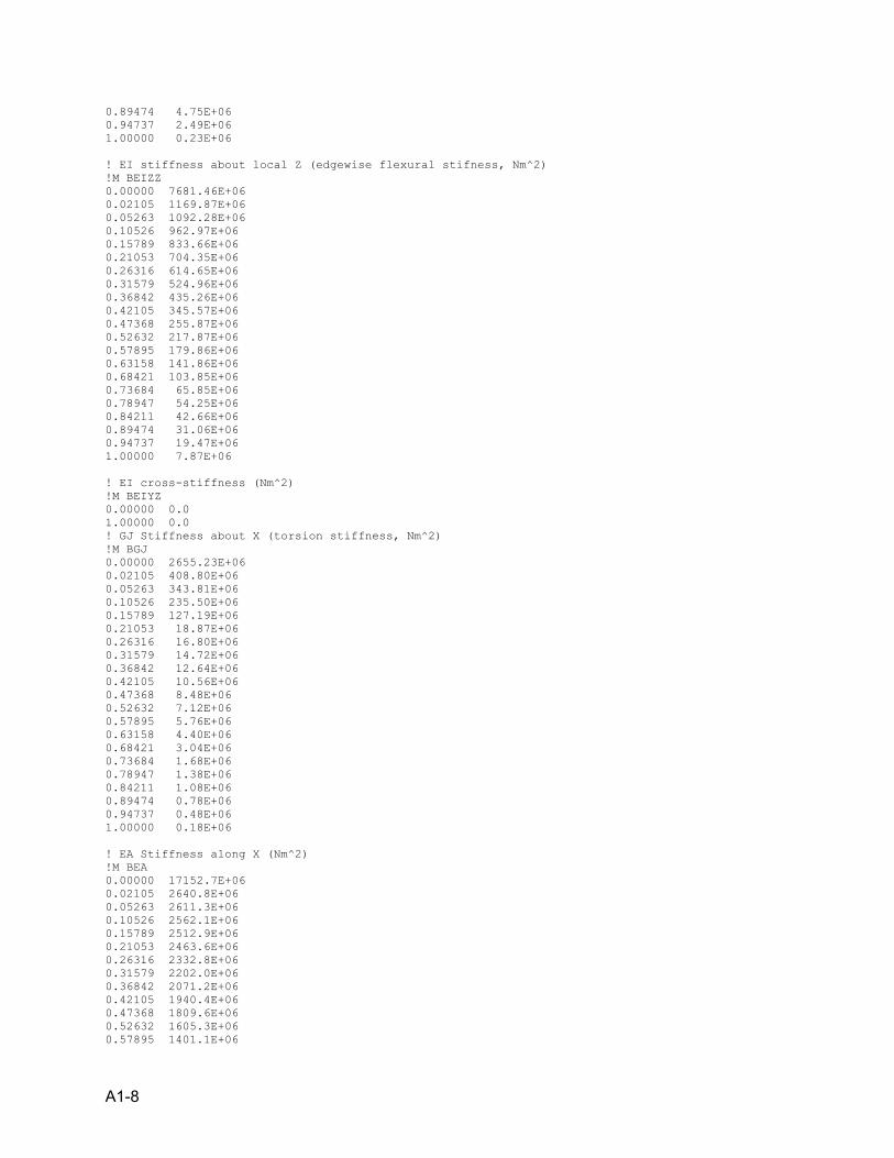
A1-8

0.89474 4.75E+06 0.94737 2.49E+06 1.00000 0.23E+06 ! EI stiffness about local Z (edgewise flexural stifness, Nm^2) !M BEIZZ 0.00000 7681.46E+06 0.02105 1169.87E+06 0.05263 1092.28E+06 0.10526 962.97E+06 0.15789 833.66E+06 0.21053 704.35E+06 0.26316 614.65E+06 0.31579 524.96E+06 0.36842 435.26E+06 0.42105 345.57E+06 0.47368 255.87E+06 0.52632 217.87E+06 0.57895 179.86E+06 0.63158 141.86E+06 0.68421 103.85E+06 0.73684 65.85E+06 0.78947 54.25E+06 0.84211 42.66E+06 0.89474 31.06E+06 0.94737 19.47E+06 1.00000 7.87E+06 ! EI cross-stiffness (Nm^2) !M BEIYZ 0.00000 0.0 1.00000 0.0 ! GJ Stiffness about X (torsion stiffness, Nm^2) !M BGJ 0.00000 2655.23E+06 0.02105 408.80E+06 0.05263 343.81E+06 0.10526 235.50E+06 0.15789 127.19E+06 0.21053 18.87E+06 0.26316 16.80E+06 0.31579 14.72E+06 0.36842 12.64E+06 0.42105 10.56E+06 0.47368 8.48E+06 0.52632 7.12E+06 0.57895 5.76E+06 0.63158 4.40E+06 0.68421 3.04E+06 0.73684 1.68E+06 0.78947 1.38E+06 0.84211 1.08E+06 0.89474 0.78E+06 0.94737 0.48E+06 1.00000 0.18E+06 ! EA Stiffness along X (Nm^2) !M BEA 0.00000 17152.7E+06 0.02105 2640.8E+06 0.05263 2611.3E+06 0.10526 2562.1E+06 0.15789 2512.9E+06 0.21053 2463.6E+06 0.26316 2332.8E+06 0.31579 2202.0E+06 0.36842 2071.2E+06 0.42105 1940.4E+06 0.47368 1809.6E+06 0.52632 1605.3E+06 0.57895 1401.1E+06

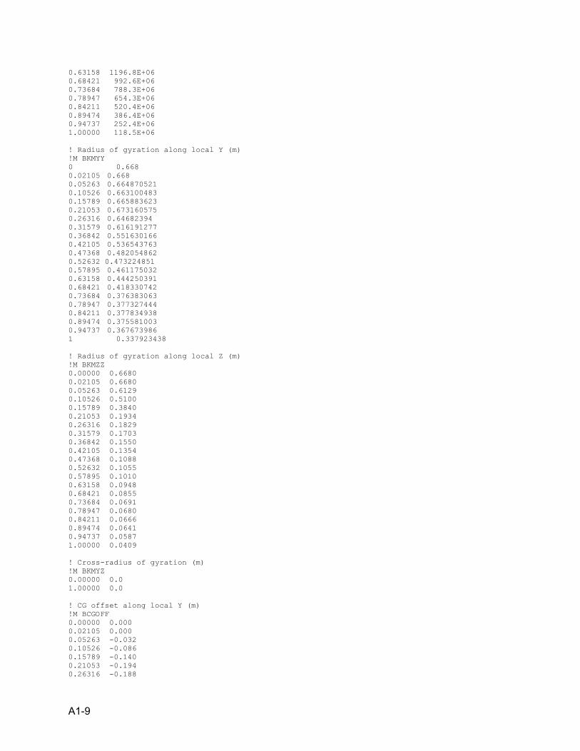
A1-9

0.63158 1196.8E+06 0.68421 992.6E+06 0.73684 788.3E+06 0.78947 654.3E+06 0.84211 520.4E+06 0.89474 386.4E+06 0.94737 252.4E+06 1.00000 118.5E+06 ! Radius of gyration along local Y (m) !M BKMYY 0 0.668 0.02105 0.668 0.05263 0.664870521 0.10526 0.663100483 0.15789 0.665883623 0.21053 0.673160575 0.26316 0.64682394 0.31579 0.616191277 0.36842 0.551630166 0.42105 0.536543763 0.47368 0.482054862 0.52632 0.473224851 0.57895 0.461175032 0.63158 0.444250391 0.68421 0.418330742 0.73684 0.376383063 0.78947 0.377327444 0.84211 0.377834938 0.89474 0.375581003 0.94737 0.367673986 1 0.337923438 ! Radius of gyration along local Z (m) !M BKMZZ 0.00000 0.6680 0.02105 0.6680 0.05263 0.6129 0.10526 0.5100 0.15789 0.3840 0.21053 0.1934 0.26316 0.1829 0.31579 0.1703 0.36842 0.1550 0.42105 0.1354 0.47368 0.1088 0.52632 0.1055 0.57895 0.1010 0.63158 0.0948 0.68421 0.0855 0.73684 0.0691 0.78947 0.0680 0.84211 0.0666 0.89474 0.0641 0.94737 0.0587 1.00000 0.0409 ! Cross-radius of gyration (m) !M BKMYZ 0.00000 0.0 1.00000 0.0 ! CG offset along local Y (m) !M BCGOFF 0.00000 0.000 0.02105 0.000 0.05263 -0.032 0.10526 -0.086 0.15789 -0.140 0.21053 -0.194 0.26316 -0.188

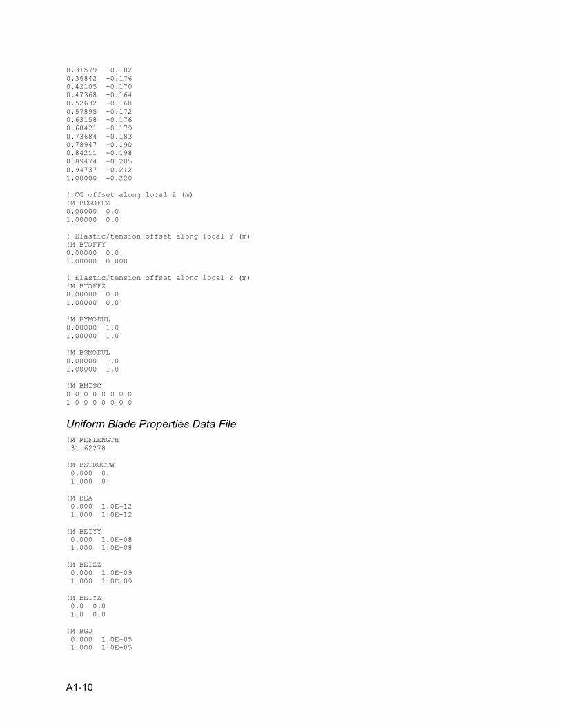
A1-10

0.31579 -0.182 0.36842 -0.176 0.42105 -0.170 0.47368 -0.164 0.52632 -0.168 0.57895 -0.172 0.63158 -0.176 0.68421 -0.179 0.73684 -0.183 0.78947 -0.190 0.84211 -0.198 0.89474 -0.205 0.94737 -0.212 1.00000 -0.220 ! CG offset along local Z (m) !M BCGOFFZ 0.00000 0.0 1.00000 0.0 ! Elastic/tension offset along local Y (m) !M BTOFFY 0.00000 0.0 1.00000 0.000 ! Elastic/tension offset along local Z (m) !M BTOFFZ 0.00000 0.0 1.00000 0.0 !M BYMODUL 0.00000 1.0 1.00000 1.0 !M BSMODUL 0.00000 1.0 1.00000 1.0 !M BMISC 0 0 0 0 0 0 0 0 1 0 0 0 0 0 0 0

Uniform Blade Properties Data File !M REFLENGTH 31.62278 !M BSTRUCTW 0.000 0. 1.000 0. !M BEA 0.000 1.0E+12 1.000 1.0E+12 !M BEIYY 0.000 1.0E+08 1.000 1.0E+08 !M BEIZZ 0.000 1.0E+09 1.000 1.0E+09 !M BEIYZ 0.0 0.0 1.0 0.0 !M BGJ 0.000 1.0E+05 1.000 1.0E+05

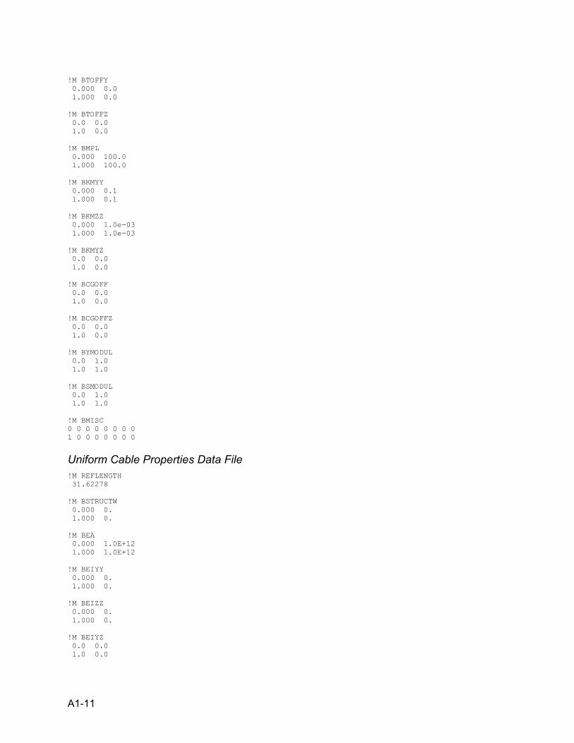
A1-11

!M BTOFFY 0.000 0.0 1.000 0.0 !M BTOFFZ 0.0 0.0 1.0 0.0 !M BMPL 0.000 100.0 1.000 100.0 !M BKMYY 0.000 0.1 1.000 0.1 !M BKMZZ 0.000 1.0e-03 1.000 1.0e-03 !M BKMYZ 0.0 0.0 1.0 0.0 !M BCGOFF 0.0 0.0 1.0 0.0 !M BCGOFFZ 0.0 0.0 1.0 0.0 !M BYMODUL 0.0 1.0 1.0 1.0 !M BSMODUL 0.0 1.0 1.0 1.0 !M BMISC 0 0 0 0 0 0 0 0 1 0 0 0 0 0 0 0

Uniform Cable Properties Data File !M REFLENGTH 31.62278 !M BSTRUCTW 0.000 0. 1.000 0. !M BEA 0.000 1.0E+12 1.000 1.0E+12 !M BEIYY 0.000 0. 1.000 0. !M BEIZZ 0.000 0. 1.000 0. !M BEIYZ 0.0 0.0 1.0 0.0

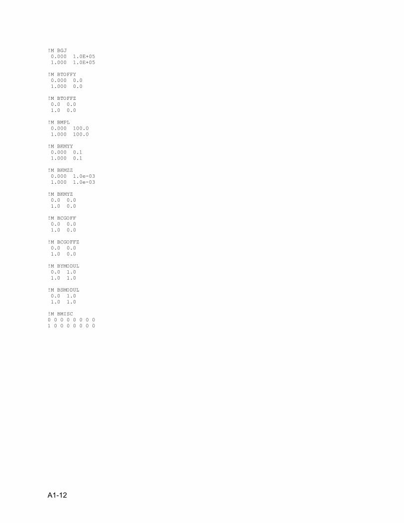
A1-12

!M BGJ 0.000 1.0E+05 1.000 1.0E+05 !M BTOFFY 0.000 0.0 1.000 0.0 !M BTOFFZ 0.0 0.0 1.0 0.0 !M BMPL 0.000 100.0 1.000 100.0 !M BKMYY 0.000 0.1 1.000 0.1 !M BKMZZ 0.000 1.0e-03 1.000 1.0e-03 !M BKMYZ 0.0 0.0 1.0 0.0 !M BCGOFF 0.0 0.0 1.0 0.0 !M BCGOFFZ 0.0 0.0 1.0 0.0 !M BYMODUL 0.0 1.0 1.0 1.0 !M BSMODUL 0.0 1.0 1.0 1.0 !M BMISC 0 0 0 0 0 0 0 0 1 0 0 0 0 0 0 0

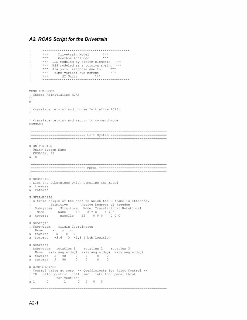
A2-1

A2. RCAS Script for the Drivetrain ! ********************************************* ! *** Drivetrain Model *** ! *** Gearbox included *** ! *** LSS modeled by finite elements *** ! *** HSS modeled as a torsion spring *** ! *** Analysis: response due to *** ! *** time-variant hub moment *** ! *** SI Units *** ! ********************************************* MENU RCASROOT ! Choose Reinitialize RCAS 11 E ! <carriage return> and choose Initialize RCAS... 1 ! <carriage return> and return to command mode COMMAND !====================================================================== !============================ Unit System ============================= !====================================================================== S UNITSYSTEM ! Unity System Name ! ENGLISH, SI a SI !====================================================================== !============================ MODEL =================================== !====================================================================== ! S SUBSYSIDS ! List the subsystems which comprise the model a towerss a rotorss S GFRAMEORIG ! G frame origin of the node to which the G frame is attached. ! Primitive Active Degrees of Freedom ! Subsystem Structure Node Translational Rotational ! Name Name ID X Y Z X Y Z a towerss nacelle 22 0 0 0 0 0 0 s ssorigin ! Subsystem Origin Coordinates ! Name x y z a towerss 0 0 0 a rotorss -3.6 0 -1.6 ! hub location s ssorient ! Subsystem rotation 1 rotation 2 rotation 3 ! Name axis angle(deg) axis angle(deg) axis angle(deg) a towerss 2 90 0 0 0 0 a rotorss 2 90 0 0 0 0 S CONTROLMIXER ! Control Value at zero -- Coefficients for Pilot Control -- ! ID pilot control coll used latc lonc pedal throt ! for mechload a 1 0 1 0 0 0 0 !======================================================================

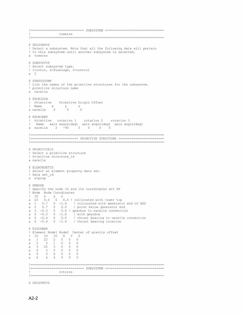
A2-2

!============================ SUBSYSTEM =============================== ! towerss !====================================================================== S SELSUBSYS ! Select a subsystem. Note that all the following data will pertain ! to this subsystem until another subsystem is selected. a towerss S SUBSYSTYP ! Select subsystem type. ! 1=rotor, 2=fuselage, 3=control a 2 S SUBSYSCOMP ! List the names of the primitive structures for the subsystem. ! primitive structure name a nacelle S PSORIGIN ! Primitive Primitive Origin Offset ! Name x y z a nacelle 0 0 0 S PSORIENT ! Primitive rotation 1 rotation 2 rotation 3 ! Name axis angle(deg) axis angle(deg) axis angle(deg) a nacelle 2 -90 0 0 0 0 !====================================================================== !========================= PRIMITIVE STRUCTURE ======================== !====================================================================== S PRIMITIVEID ! Select a primitive structure ! Primitive structure_id a nacelle S ELDATASETID ! Select an element property data set. ! Data set_id a elprop S FENODE ! Specify the node ID and its coordinates wrt PS ! Node Node Coordinates ! ID x y z a 22 0.0 0 0.0 ! collocated with tower top a 1 0.7 0 -1.6 ! collocated with generator end of HSS a 2 0.7 0 0.0 ! point below generator end a 3 -0.3 0 0.0 ! gearbox to nacelle connection a 4 -0.3 0 -1.6 ! with gearbox a 5 -0.4 0 0.0 ! thrust bearing to nacelle connection a 6 -0.4 0 -1.6 ! thrust bearing location S RIGIDBAR ! Element Node1 Node2 Center of gravity offset ! ID ID ID X Y Z a 1 22 2 0 0 0 a 2 2 1 0 0 0 a 3 22 3 0 0 0 a 4 3 5 0 0 0 a 5 5 6 0 0 0 a 6 6 4 0 0 0 !====================================================================== !============================ SUBSYSTEM =============================== ! rotorss !====================================================================== S SELSUBSYS

A2-3

! Select a subsystem. Note that all the following data will pertain ! to this subsystem until another subsystem is selected. a rotorss S SUBSYSTYP ! Select subsystem type. ! 1=rotor, 2=towersslage, 3=control a 1 S SUBSYSCOMP ! List the names of the primitive structures for the subsystem. ! Primitive Structure ! Name a rshaft !Rotating shaft prim. struct S CORNODE ! Identify Center Of Rotation Node ! Prim. struct. Drivetrain ! ID Node_ID A rshaft 10 S BLADECOMP ! Blade Primitive Structure Name(s) ! Index 1 2 3 4 5 6 7 a 1 rshaft -- -- -- -- -- -- s psorigin ! Primitive Primitive Origin Offset ! Name x y z a rshaft 0 0 0.0 s psorient ! Primitive rotation 1 rotation 2 rotation 3 ! Name axis angle(deg) axis angle(deg) axis angle(deg) a rshaft 2 -90 0 0 0 0 !rpm=1800 !gr = 87.965 !rpm_rotor = 1800/87.965 =20.4627 ==> omega = 2.1428 S ROTORPARAM ! Rotor Rotational Speed (rad/sec) a 2.1428 !====================================================================== !========================= PRIMITIVE STRUCTURE ======================== ! rshaft !====================================================================== S PRIMITIVEID ! Select a primitive structure ! Primitive structure_id a rshaft S ELDATASETID ! Select an element property data set. ! Data set_id a elprop S FENODE ! Specify the node ID and its coordinates wrt PS ! Node Node Coordinates ! ID x y z a 1 0.0 0 0 ! Hub location a 5 3.2 0 0 ! Thrust bearing (hub side) a 6 3.2 0 0 ! Thrust bearing (gearbox side) a 7 3.3 0 0 ! Gear box (LSS side) a 8 3.3 0 0 ! Gear box (HSS side)B a 9 4.2 0 0 ! a 10 4.3 0 0 ! drivetrain generator S SEGEARBOX

A2-4

! Elem. Nominal Moment of Damping Fixed System Connection Node ! ID Omega Inertia Coefficient Subsys Prim_Str Node_ID a 1 2.1428 2.1 .01 towerss nacelle 4 !A N ! Row Elem. Child Gear Child Shaft Orientation Angles ! ID ID Node ID Ratio Phi Theta Psi a 1 1 7 1 0 0 0 a 2 1 8 87.965 0 0 0 S IDEALBEARING ! Elem. Node1 Node2 Axis of Connect to fixed system ! ID ID ID Bearing Subsys Prim_Str Node_ID a 2 5 6 X towerss nacelle 6 !E S RIGIDBAR ! Element Node1 Node2 Center of gravity offset ! ID ID ID X Y Z !!a 3 1 5 0 0 0 ! lss 1 !!a 4 6 7 0 0 0 ! lss 2 a 5 9 10 0 0 0 ! hss 1 N ! ID Mass Ixx Ixy Ixz Iyy Iyz Izz a 3 100 2.0e11 0 0 0 0 0 ! lss inertia 2.0e9 !a 3 100 2.0e11 0 0 0 0 0 ! lss inertia a 5 10 1.0e3 0 0 0 0 0 ! hss inertia !---- S NLBEAMDEF !Elem 1st 2nd Shape NGauss MatProp End Node Active DOFs ! ID Node Node Func ID Points ID ue v w phi w' v' a 4 6 7 1 6 11 1 0 0 1 0 0 a 14 1 5 1 6 11 1 0 0 1 0 0 N N !Specify the structural property data table (file) ! Element Refernce Property ! ID origin Filename a 4 3.2 SHAFT.TAB a 14 3.2 SHAFT.TAB !---- S SPRELE !Element Node1 Node2 Trans./Rot. Type Linear stiffness ! ID ID ID (TR/RX/RY/RZ) (L/N) coefficient a 6 8 9 RX L 3.62E+6 !dt stiffness ? S DMPELE ! Element Node1 Node2 Trans./Rot. Type Linear Damping ! ID ID ID (TR/RX/RY/RZ) (L/N) coefficient a 7 8 9 RX L 0000 ! dt damper 2000 S RBMELE ! Generate rigid body mass element. ! ELID, node ID, prop ID A 10 1 2 SCREEN MECHLOAD ! Elem Node Steady Load Direction Coord. Frame Periodic ! ID ID Amplitude (FX|FY|FZ|MX|MY|MZ) (EL|PS) Input ID a 31 1 0 MX EL 0 S CONTROLCONNECT ! Control Swashplate Swashplate Element Type Element ! ID or Direct Phase(deg) (HIN/AUX/ENG ...) or ACP ID a 1 DIRECT 0.0 MLD 31 !====================================================================== !============== Rotating to Nonrotating Connection ==================== !======================================================================

A2-5

S ROTNONCONST !Cnstr. Subsys. Primit. Node Subsys. Primit. Node ! ID Name Name ID Name Name ID a 1 towerss nacelle 1 rotorss rshaft 10 !====================================================================== !======================== STRUCTURAL PROPERTIES ======================= ! ELPROP !====================================================================== S ELEPROPID ! Add the name of an element property data set. ! element_prop_id a elprop S RBMPRP ! Prop Elem. Center Mass Offset --- Mass Moment of Inertia Matrix --- ! ID Mass X Y Z Ixx, Ixy Ixz Iyy Iyz Izz A 1 1.e-7 0 0 0 0 0 0 0 0 0 A 2 50 0 0 0 1000 0 0 9000 0 10000 S NLBSHAPE ! NLB Shape Function Orders ! Shape fn ID Axial Bending Torsion A 1 1 0 1 S MATPROPER ! Input material properties (E, G) ! material id, Young's Modulus, shear Modulus a 11 1.0 1.0 !====================================================================== !====================================================================== ! END OF MODEL DEFINITION !====================================================================== !====================================================================== !====================================================================== !========================== ANALYSIS DATA ============================= !====================================================================== S SELANALYSIS ! Case ID Trim Mane Stab Init ----- Scope Script ----- ! (0:3) (0:1) (0:1) Cond File Name A 1 0 1 0 D NO N ! Case ID Case Title (Maximum 30 Characters) a 1 wttest S INITCOND ! Initial Controls ! coll used latc lonc pedal throt ! for Mechload a 0 0 0 0 0 S SYSTEMFLAGS ! Global element formulation flags (1=Yes, 0=No) ! Gravity Aero ! Effects Effects a 0 0 S CONVERGETOL ! # of # of # of Displ. Tolerance veloc tolerance Min. ! Trim PSol Time (Trans, Rot) (Trans, Rot) # of ! Iter Iter Step (ft) (rad) (ft/sec)(rad/sec) PS Rev a 10 4 36 0.005 0.01 1.0 0.01 5 SCREEN INTEGPARAM !No. of| Newmark Constants| HHT | Displace. | Velocity | Relax. !Iter. | Alpha | Delta | Param | Tol | Tol | Factor a 20 .25 .5 -.03 1.e-6 1.e-5 1.0

A2-6

!====================================================================== !========================= STABILITY DATA ============================= S linearoption ! Perturb. Number of Control Gust Identical Reduction Averaging ! Delta Azim/Rev Option Opt. Blade Opt. Option Option a 0.001 1 0 0 0 0 S CCEANALYSIS !Eigenanalysis Number of Transient Frequency Mean Squared ! Option Modes Response Opt. Response Opt. Random Response a 1 0 0 0 0 !====================================================================== !========================== MANEUVER DATA ============================= !====================================================================== S MANEUVERINPUT !Number of Time Time Step ! Steps (sec) a 10000 .1 5 N !Row INPUT Step Number Amp1 Amp2 Freq1 Freq2 Phase ! ID ID Start End (Hz) (HZ) (Deg) a 1 coll 1 4000 1.E+7 1.E+7 0 0 0.0 S MANEUVEROUTPUT ! Row Subsystem Prim. Struc. output ! ID Name Name category a 1 all all System_Dynamic.Response a 2 all all Internal.Loads !====================================================================== !========================= OUTPUT SLECTION============================= S PERIODICOUTPUT ! Row Subsystem Prim. Struc. output ! ID Name Name category a 1 all all internal.loads a 2 all all airloads EXIT COMMAND MENU RUNANALYSIS

Low-Speed Shaft Properties Data File ! Structural properties for the shaft of a 1.5-MW turbine (provided by C. Hansen) ! Note: "!M PropName" is an identifier telling RCAS that the subsequent data set belongs to the category "PropName". ! The order of data sets is unimportant. ! Reference length (m) !M REFLENGTH 3.3 !M BSTRUCTW 0.000 0. 1.000 0. !M BEA 0.000 1.0E+14 1.000 1.0E+14 !M BEIYY 0.000 1.0E+09

A2-7

1.000 1.0E+09 !M BEIZZ 0.000 1.0E+09 1.000 1.0E+09 !M BEIYZ 0.0 0.0 1.0 0.0 !M BGJ 0.000 7.0E+08 1.000 7.0E+08 !M BTOFFY 0.000 0.0 1.000 0.0 !M BTOFFZ 0.0 0.0 1.0 0.0 !M BMPL 0.000 1.0 1.000 1.0 !M BKMYY 0.000 0.01 1.000 0.01 !M BKMZZ 0.000 0.01 1.000 0.01 !M BKMYZ 0.0 0.0 1.0 0.0 !M BCGOFF 0.0 0.0 1.0 0.0 !M BCGOFFZ 0.0 0.0 1.0 0.0 !M BYMODUL 0.0 1.0 1.0 1.0 !M BSMODUL 0.0 1.0 1.0 1.0 !M BMISC 0 0 0 0 0 0 0 0 1 0 0 0 0 0 0 0

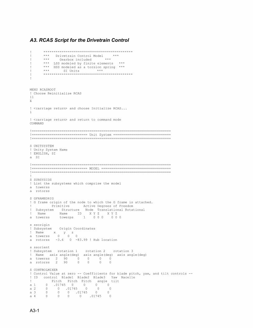
A3-1

A3. RCAS Script for the Drivetrain Control ! ********************************************* ! *** Drivetrain Control Model *** ! *** Gearbox included *** ! *** LSS modeled by finite elements *** ! *** HSS modeled as a torsion spring *** ! *** SI Units *** ! ********************************************* ! MENU RCASROOT ! Choose Reinitialize RCAS 11 E ! <carriage return> and choose Initialize RCAS... 1 ! <carriage return> and return to command mode COMMAND !====================================================================== !============================ Unit System ============================= !====================================================================== S UNITSYSTEM ! Unity System Name ! ENGLISH, SI a SI !====================================================================== !============================ MODEL =================================== !====================================================================== ! S SUBSYSIDS ! List the subsystems which comprise the model a towerss a rotorss S GFRAMEORIG ! G frame origin of the node to which the G frame is attached. ! Primitive Active Degrees of Freedom ! Subsystem Structure Node Translational Rotational ! Name Name ID X Y Z X Y Z a towerss towerps 1 0 0 0 0 0 0 s ssorigin ! Subsystem Origin Coordinates ! Name x y z a towerss 0 0 0 a rotorss -3.6 0 -83.99 ! Hub location s ssorient ! Subsystem rotation 1 rotation 2 rotation 3 ! Name axis angle(deg) axis angle(deg) axis angle(deg) a towerss 2 90 0 0 0 0 a rotorss 2 90 0 0 0 0 S CONTROLMIXER ! Control Value at zero -- Coefficients for blade pitch, yaw, and tilt controls -- ! ID control Blade1 Blade2 Blade3 Yaw Nacelle ! Pitch Pitch Pitch angle tilt a 1 0 .01745 0 0 0 0 a 2 0 0 .01745 0 0 0 a 3 0 0 0 .01745 0 0 a 4 0 0 0 0 .01745 0

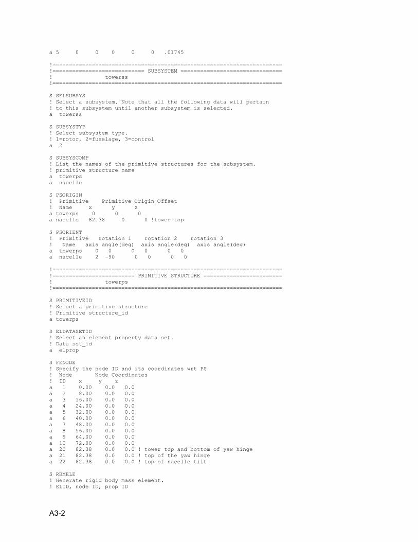
A3-2

a 5 0 0 0 0 0 .01745 !====================================================================== !============================ SUBSYSTEM =============================== ! towerss !====================================================================== S SELSUBSYS ! Select a subsystem. Note that all the following data will pertain ! to this subsystem until another subsystem is selected. a towerss S SUBSYSTYP ! Select subsystem type. ! 1=rotor, 2=fuselage, 3=control a 2 S SUBSYSCOMP ! List the names of the primitive structures for the subsystem. ! primitive structure name a towerps a nacelle S PSORIGIN ! Primitive Primitive Origin Offset ! Name x y z a towerps 0 0 0 a nacelle 82.38 0 0 !tower top S PSORIENT ! Primitive rotation 1 rotation 2 rotation 3 ! Name axis angle(deg) axis angle(deg) axis angle(deg) a towerps 0 0 0 0 0 0 a nacelle 2 -90 0 0 0 0 !====================================================================== !========================= PRIMITIVE STRUCTURE ======================== ! towerps !====================================================================== S PRIMITIVEID ! Select a primitive structure ! Primitive structure_id a towerps S ELDATASETID ! Select an element property data set. ! Data set_id a elprop S FENODE ! Specify the node ID and its coordinates wrt PS ! Node Node Coordinates ! ID x y z a 1 0.00 0.0 0.0 a 2 8.00 0.0 0.0 a 3 16.00 0.0 0.0 a 4 24.00 0.0 0.0 a 5 32.00 0.0 0.0 a 6 40.00 0.0 0.0 a 7 48.00 0.0 0.0 a 8 56.00 0.0 0.0 a 9 64.00 0.0 0.0 a 10 72.00 0.0 0.0 a 20 82.38 0.0 0.0 ! tower top and bottom of yaw hinge a 21 82.38 0.0 0.0 ! top of the yaw hinge a 22 82.38 0.0 0.0 ! top of nacelle tilt S RBMELE ! Generate rigid body mass element. ! ELID, node ID, prop ID

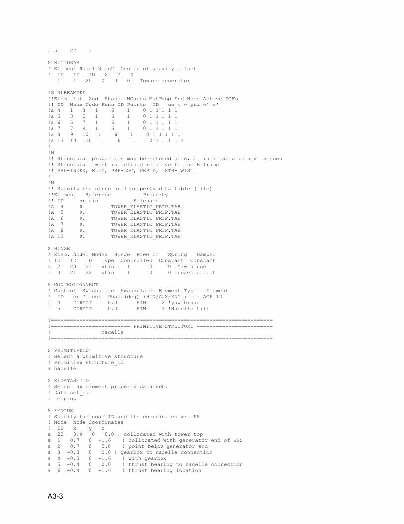
A3-3

a 51 22 1 S RIGIDBAR ! Element Node1 Node2 Center of gravity offset ! ID ID ID X Y Z a 1 1 20 0 0 0 ! Toward generator !S NLBEAMDEF !!Elem 1st 2nd Shape NGauss MatProp End Node Active DOFs !! ID Node Node Func ID Points ID ue v w phi w' v' !a 4 1 3 1 6 1 0 1 1 1 1 1 !a 5 3 5 1 6 1 0 1 1 1 1 1 !a 6 5 7 1 6 1 0 1 1 1 1 1 !a 7 7 9 1 6 1 0 1 1 1 1 1 !a 8 9 10 1 6 1 0 1 1 1 1 1 !a 13 10 20 1 6 1 0 1 1 1 1 1 ! !N !! Structural properties may be entered here, or in a table in next screen !! Structural twist is defined relative to the E frame !! PRP-INDEX, ELID, PRP-LOC, PRPID, STR-TWIST ! !N !! Specify the structural property data table (file) !!Element Refernce Property !! ID origin Filename !A 4 0. TOWER_ELASTIC_PROP.TAB !A 5 0. TOWER_ELASTIC_PROP.TAB !A 6 0. TOWER_ELASTIC_PROP.TAB !A 7 0. TOWER_ELASTIC_PROP.TAB !A 8 0. TOWER_ELASTIC_PROP.TAB !A 13 0. TOWER_ELASTIC_PROP.TAB S HINGE ! Elem. Node1 Node2 Hinge Free or Spring Damper ! ID ID ID Type Controlled Constant Constant a 2 20 21 xhin 1 0 0 !Yaw hinge a 3 21 22 yhin 1 0 0 !ncaelle tilt S CONTROLCONNECT ! Control Swashplate Swashplate Element Type Element ! ID or Direct Phase(deg) (HIN/AUX/ENG ) or ACP ID a 4 DIRECT 0.0 HIN 2 !yaw hinge a 5 DIRECT 0.0 HIN 3 !Nacelle tilt !====================================================================== !========================= PRIMITIVE STRUCTURE ======================== ! nacelle !====================================================================== S PRIMITIVEID ! Select a primitive structure ! Primitive structure_id a nacelle S ELDATASETID ! Select an element property data set. ! Data set_id a elprop S FENODE ! Specify the node ID and its coordinates wrt PS ! Node Node Coordinates ! ID x y z a 22 0.0 0 0.0 ! collocated with tower top a 1 0.7 0 -1.6 ! collocated with generator end of HSS a 2 0.7 0 0.0 ! point below generator end a 3 -0.3 0 0.0 ! gearbox to nacelle connection a 4 -0.3 0 -1.6 ! with gearbox a 5 -0.4 0 0.0 ! thrust bearing to nacelle connection a 6 -0.4 0 -1.6 ! thrust bearing location

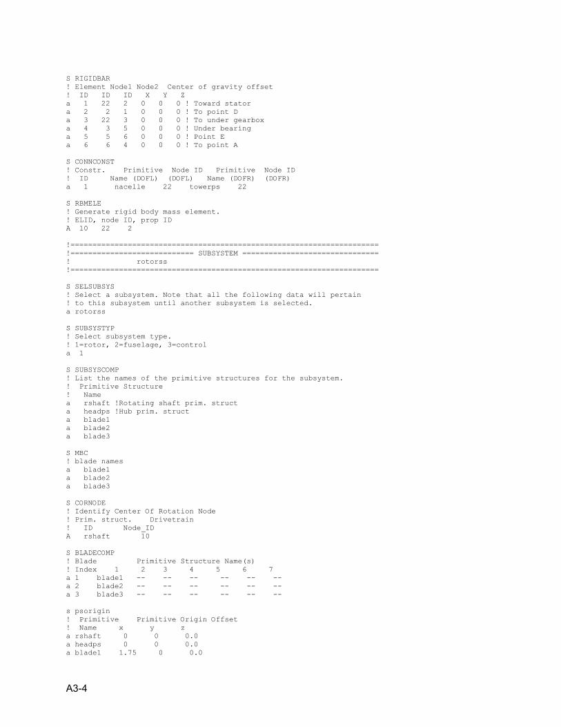
A3-4

S RIGIDBAR ! Element Node1 Node2 Center of gravity offset ! ID ID ID X Y Z a 1 22 2 0 0 0 ! Toward stator a 2 2 1 0 0 0 ! To point D a 3 22 3 0 0 0 ! To under gearbox a 4 3 5 0 0 0 ! Under bearing a 5 5 6 0 0 0 ! Point E a 6 6 4 0 0 0 ! To point A S CONNCONST ! Constr. Primitive Node ID Primitive Node ID ! ID Name (DOFL) (DOFL) Name (DOFR) (DOFR) a 1 nacelle 22 towerps 22 S RBMELE ! Generate rigid body mass element. ! ELID, node ID, prop ID A 10 22 2 !====================================================================== !============================ SUBSYSTEM =============================== ! rotorss !====================================================================== S SELSUBSYS ! Select a subsystem. Note that all the following data will pertain ! to this subsystem until another subsystem is selected. a rotorss S SUBSYSTYP ! Select subsystem type. ! 1=rotor, 2=fuselage, 3=control a 1 S SUBSYSCOMP ! List the names of the primitive structures for the subsystem. ! Primitive Structure ! Name a rshaft !Rotating shaft prim. struct a headps !Hub prim. struct a blade1 a blade2 a blade3 S MBC ! blade names a blade1 a blade2 a blade3 S CORNODE ! Identify Center Of Rotation Node ! Prim. struct. Drivetrain ! ID Node_ID A rshaft 10 S BLADECOMP ! Blade Primitive Structure Name(s) ! Index 1 2 3 4 5 6 7 a 1 blade1 -- -- -- -- -- -- a 2 blade2 -- -- -- -- -- -- a 3 blade3 -- -- -- -- -- -- s psorigin ! Primitive Primitive Origin Offset ! Name x y z a rshaft 0 0 0.0 a headps 0 0 0.0 a blade1 1.75 0 0.0

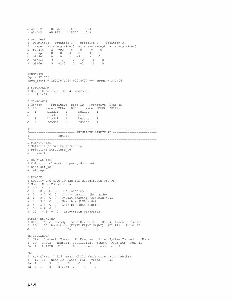
A3-5

a blade2 -0.875 -1.5155 0.0 a blade3 -0.875 1.5155 0.0 s psorient ! Primitive rotation 1 rotation 2 rotation 3 ! Name axis angle(deg) axis angle(deg) axis angle(deg) a rshaft 2 -90 0 0 0 0 a headps 0 0 0 0 0 0 a blade1 0 0 2 -2 0 0 a blade2 3 -120 2 -2 0 0 a blade3 3 -240 2 -2 0 0 !rpm=1800 !gr = 87.965 !rpm_rotor = 1800/87.965 =20.4627 ==> omega = 2.1428 S ROTORPARAM ! Rotor Rotational Speed (rad/sec) a 2.1428 S CONNCONST ! Constr. Primitive Node ID Primitive Node ID ! ID Name (DOFL) (DOFL) Name (DOFR) (DOFR) a 1 blade1 1 headps 1 a 2 blade2 1 headps 2 a 3 blade3 1 headps 3 a 4 headps 8 rshaft 1 !====================================================================== !========================= PRIMITIVE STRUCTURE ======================== ! rshaft !====================================================================== S PRIMITIVEID ! Select a primitive structure ! Primitive structure_id a rshaft S ELDATASETID ! Select an element property data set. ! Data set_id a elprop S FENODE ! Specify the node ID and its coordinates wrt PS ! Node Node Coordinates ! ID x y z a 1 0.0 0 0 ! Hub location a 5 3.2 0 0 ! Thrust bearing (hub side) a 6 3.2 0 0 ! Thrust bearing (gearbox side) a 7 3.3 0 0 ! Gear box (LSS side) a 8 3.3 0 0 ! Gear box (HSS side)B a 9 4.2 0 0 ! a 10 4.3 0 0 ! drivetrain generator SCREEN MECHLOAD ! Elem Node Steady Load Direction Coord. Frame Periodic ! ID ID Amplitude (FX|FY|FZ|MX|MY|MZ) (EL|PS) Input ID a 9 10 0 MX EL 0 !S SEGEARBOX !! Elem. Nominal Moment of Damping Fixed System Connection Node !! ID Omega Inertia Coefficient Subsys Prim_Str Node_ID !a 1 2.1428 2.1 .00 towerss nacelle 4 !N !! Row Elem. Child Gear Child Shaft Orientation Angles !! ID ID Node ID Ratio Phi Theta Psi !a 1 1 7 1 0 0 0 !a 2 1 8 87.965 0 0 0

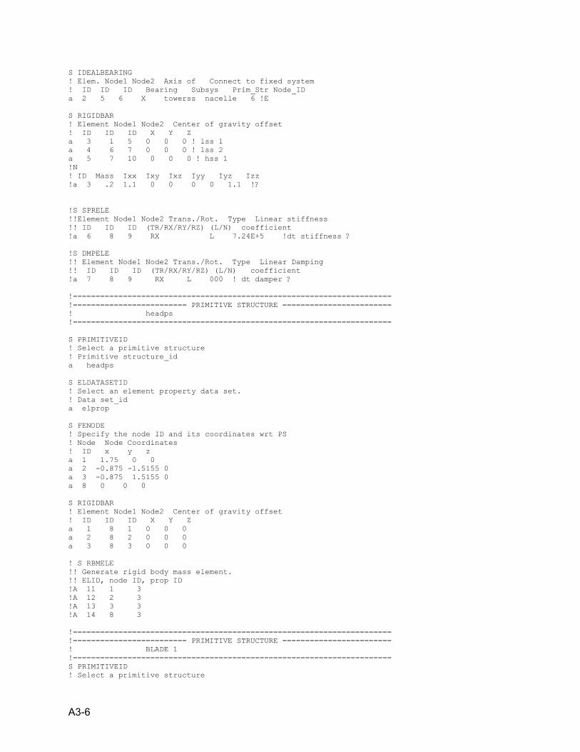
A3-6

S IDEALBEARING ! Elem. Node1 Node2 Axis of Connect to fixed system ! ID ID ID Bearing Subsys Prim_Str Node_ID a 2 5 6 X towerss nacelle 6 !E S RIGIDBAR ! Element Node1 Node2 Center of gravity offset ! ID ID ID X Y Z a 3 1 5 0 0 0 ! lss 1 a 4 6 7 0 0 0 ! lss 2 a 5 7 10 0 0 0 ! hss 1 !N ! ID Mass Ixx Ixy Ixz Iyy Iyz Izz !a 3 .2 1.1 0 0 0 0 1.1 !? !S SPRELE !!Element Node1 Node2 Trans./Rot. Type Linear stiffness !! ID ID ID (TR/RX/RY/RZ) (L/N) coefficient !a 6 8 9 RX L 7.24E+5 !dt stiffness ? !S DMPELE !! Element Node1 Node2 Trans./Rot. Type Linear Damping !! ID ID ID (TR/RX/RY/RZ) (L/N) coefficient !a 7 8 9 RX L 000 ! dt damper ? !====================================================================== !========================= PRIMITIVE STRUCTURE ======================== ! headps !====================================================================== S PRIMITIVEID ! Select a primitive structure ! Primitive structure_id a headps S ELDATASETID ! Select an element property data set. ! Data set_id a elprop S FENODE ! Specify the node ID and its coordinates wrt PS ! Node Node Coordinates ! ID x y z a 1 1.75 0 0 a 2 -0.875 -1.5155 0 a 3 -0.875 1.5155 0 a 8 0 0 0 S RIGIDBAR ! Element Node1 Node2 Center of gravity offset ! ID ID ID X Y Z a 1 8 1 0 0 0 a 2 8 2 0 0 0 a 3 8 3 0 0 0 ! S RBMELE !! Generate rigid body mass element. !! ELID, node ID, prop ID !A 11 1 3 !A 12 2 3 !A 13 3 3 !A 14 8 3 !====================================================================== !========================= PRIMITIVE STRUCTURE ======================== ! BLADE 1 !====================================================================== S PRIMITIVEID ! Select a primitive structure

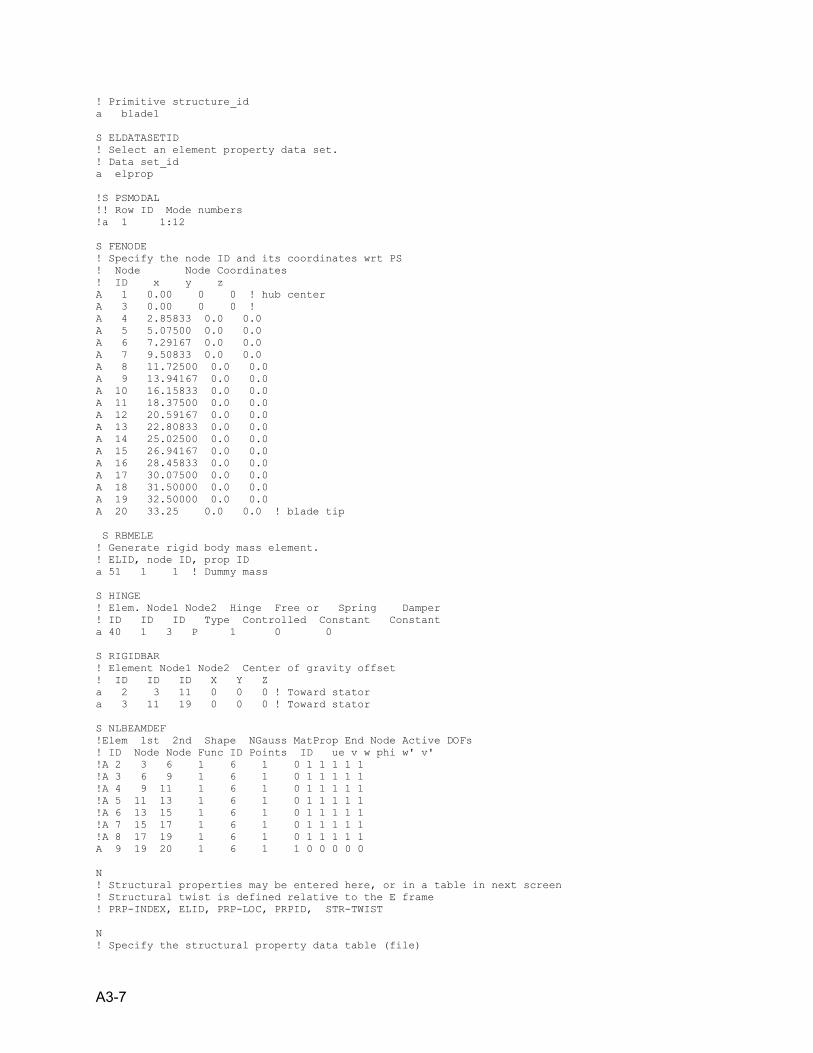
A3-7

! Primitive structure_id a blade1 S ELDATASETID ! Select an element property data set. ! Data set_id a elprop !S PSMODAL !! Row ID Mode numbers !a 1 1:12 S FENODE ! Specify the node ID and its coordinates wrt PS ! Node Node Coordinates ! ID x y z A 1 0.00 0 0 ! hub center A 3 0.00 0 0 ! A 4 2.85833 0.0 0.0 A 5 5.07500 0.0 0.0 A 6 7.29167 0.0 0.0 A 7 9.50833 0.0 0.0 A 8 11.72500 0.0 0.0 A 9 13.94167 0.0 0.0 A 10 16.15833 0.0 0.0 A 11 18.37500 0.0 0.0 A 12 20.59167 0.0 0.0 A 13 22.80833 0.0 0.0 A 14 25.02500 0.0 0.0 A 15 26.94167 0.0 0.0 A 16 28.45833 0.0 0.0 A 17 30.07500 0.0 0.0 A 18 31.50000 0.0 0.0 A 19 32.50000 0.0 0.0 A 20 33.25 0.0 0.0 ! blade tip S RBMELE ! Generate rigid body mass element. ! ELID, node ID, prop ID a 51 1 1 ! Dummy mass S HINGE ! Elem. Node1 Node2 Hinge Free or Spring Damper ! ID ID ID Type Controlled Constant Constant a 40 1 3 P 1 0 0 S RIGIDBAR ! Element Node1 Node2 Center of gravity offset ! ID ID ID X Y Z a 2 3 11 0 0 0 ! Toward stator a 3 11 19 0 0 0 ! Toward stator S NLBEAMDEF !Elem 1st 2nd Shape NGauss MatProp End Node Active DOFs ! ID Node Node Func ID Points ID ue v w phi w' v' !A 2 3 6 1 6 1 0 1 1 1 1 1 !A 3 6 9 1 6 1 0 1 1 1 1 1 !A 4 9 11 1 6 1 0 1 1 1 1 1 !A 5 11 13 1 6 1 0 1 1 1 1 1 !A 6 13 15 1 6 1 0 1 1 1 1 1 !A 7 15 17 1 6 1 0 1 1 1 1 1 !A 8 17 19 1 6 1 0 1 1 1 1 1 A 9 19 20 1 6 1 1 0 0 0 0 0 N ! Structural properties may be entered here, or in a table in next screen ! Structural twist is defined relative to the E frame ! PRP-INDEX, ELID, PRP-LOC, PRPID, STR-TWIST N ! Specify the structural property data table (file)

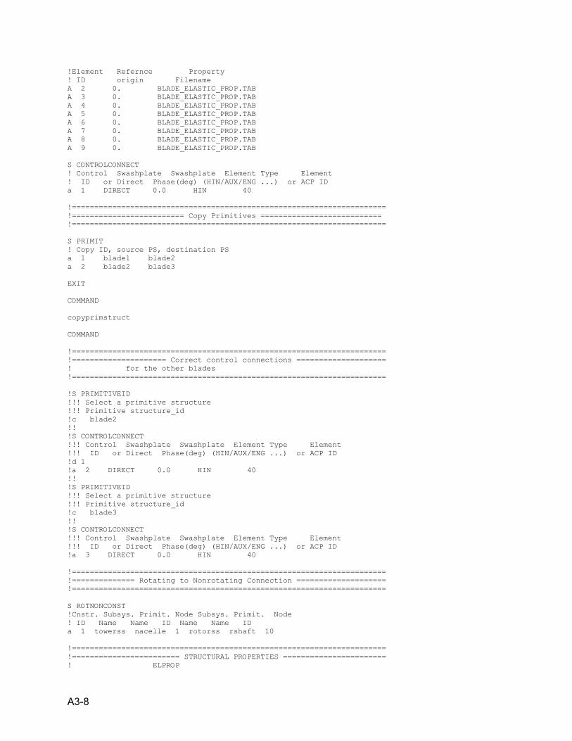
A3-8

!Element Refernce Property ! ID origin Filename A 2 0. BLADE_ELASTIC_PROP.TAB A 3 0. BLADE_ELASTIC_PROP.TAB A 4 0. BLADE_ELASTIC_PROP.TAB A 5 0. BLADE_ELASTIC_PROP.TAB A 6 0. BLADE_ELASTIC_PROP.TAB A 7 0. BLADE_ELASTIC_PROP.TAB A 8 0. BLADE_ELASTIC_PROP.TAB A 9 0. BLADE_ELASTIC_PROP.TAB S CONTROLCONNECT ! Control Swashplate Swashplate Element Type Element ! ID or Direct Phase(deg) (HIN/AUX/ENG ...) or ACP ID a 1 DIRECT 0.0 HIN 40 !====================================================================== !========================= Copy Primitives =========================== !====================================================================== S PRIMIT ! Copy ID, source PS, destination PS a 1 blade1 blade2 a 2 blade2 blade3 EXIT COMMAND copyprimstruct COMMAND !====================================================================== !===================== Correct control connections ==================== ! for the other blades !====================================================================== !S PRIMITIVEID !!! Select a primitive structure !!! Primitive structure_id !c blade2 !! !S CONTROLCONNECT !!! Control Swashplate Swashplate Element Type Element !!! ID or Direct Phase(deg) (HIN/AUX/ENG ...) or ACP ID !d 1 !a 2 DIRECT 0.0 HIN 40 !! !S PRIMITIVEID !!! Select a primitive structure !!! Primitive structure_id !c blade3 !! !S CONTROLCONNECT !!! Control Swashplate Swashplate Element Type Element !!! ID or Direct Phase(deg) (HIN/AUX/ENG ...) or ACP ID !a 3 DIRECT 0.0 HIN 40 !====================================================================== !============== Rotating to Nonrotating Connection ==================== !====================================================================== S ROTNONCONST !Cnstr. Subsys. Primit. Node Subsys. Primit. Node ! ID Name Name ID Name Name ID a 1 towerss nacelle 1 rotorss rshaft 10 !====================================================================== !======================== STRUCTURAL PROPERTIES ======================= ! ELPROP

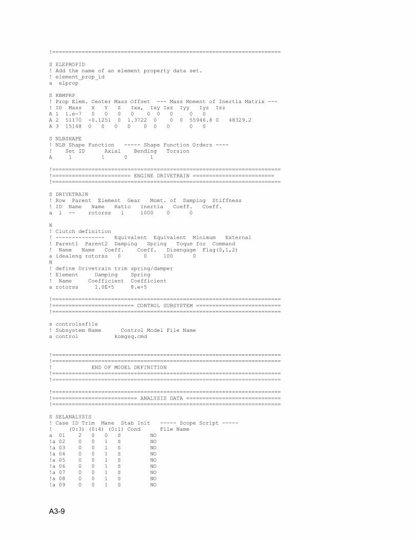
A3-9

!====================================================================== S ELEPROPID ! Add the name of an element property data set. ! element_prop_id a elprop S RBMPRP ! Prop Elem. Center Mass Offset --- Mass Moment of Inertia Matrix --- ! ID Mass X Y Z Ixx, Ixy Ixz Iyy Iyz Izz A 1 1.e-7 0 0 0 0 0 0 0 0 0 A 2 51170 -0.1251 0 1.3722 0 0 0 55946.8 0 48329.2 A 3 15148 0 0 0 0 0 0 0 0 0 S NLBSHAPE ! NLB Shape Function ----- Shape Function Orders ---- ! Set ID Axial Bending Torsion A 1 1 0 1 !====================================================================== !======================== ENGINE DRIVETRAIN ========================= !====================================================================== S DRIVETRAIN ! Row Parent Element Gear Momt. of Damping Stiffness ! ID Name Name Ratio Inertia Coeff. Coeff. a 1 -- rotorss 1 1000 0 0 N ! Clutch definition ! --------------- Equivalent Equivalent Minimum External ! Parent1 Parent2 Damping Spring Toque for Command ! Name Name Coeff. Coeff. Disengage Flag(0,1,2) a idealeng rotorss 0 0 100 0 N ! define Drivetrain trim spring/damper ! Element Damping Spring ! Name Coefficient Coefficient a rotorss 1.0E+5 8.e+5 !====================================================================== !========================= CONTROL SUBSYSTEM ========================== !====================================================================== s controlssfile ! Subsystem Name Control Model File Name a control komgsq.cmd !====================================================================== !====================================================================== ! END OF MODEL DEFINITION !====================================================================== !====================================================================== !====================================================================== !========================== ANALYSIS DATA ============================= !====================================================================== S SELANALYSIS ! Case ID Trim Mane Stab Init ----- Scope Script ----- ! (0:3) (0:4) (0:1) Cond File Name a 01 2 0 0 S NO !a 02 0 0 1 S NO !a 03 0 0 1 S NO !a 04 0 0 1 S NO !a 05 0 0 1 S NO !a 06 0 0 1 S NO !a 07 0 0 1 S NO !a 08 0 0 1 S NO !a 09 0 0 1 S NO

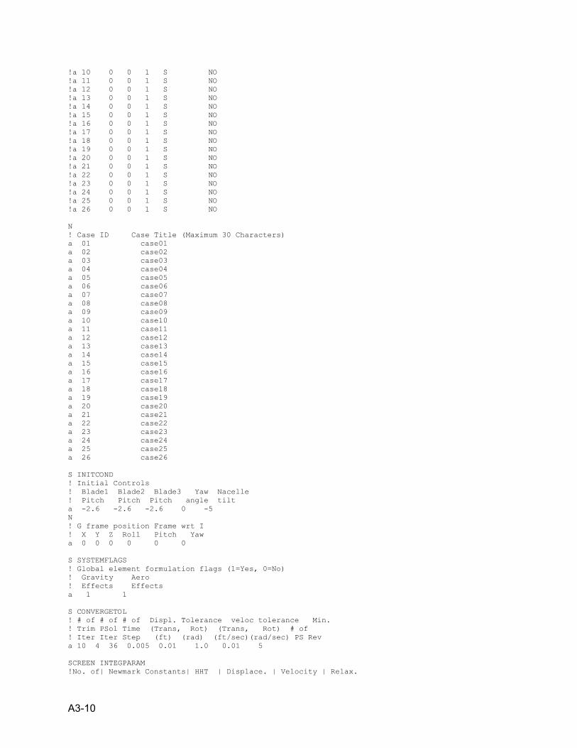
A3-10

!a 10 0 0 1 S NO !a 11 0 0 1 S NO !a 12 0 0 1 S NO !a 13 0 0 1 S NO !a 14 0 0 1 S NO !a 15 0 0 1 S NO !a 16 0 0 1 S NO !a 17 0 0 1 S NO !a 18 0 0 1 S NO !a 19 0 0 1 S NO !a 20 0 0 1 S NO !a 21 0 0 1 S NO !a 22 0 0 1 S NO !a 23 0 0 1 S NO !a 24 0 0 1 S NO !a 25 0 0 1 S NO !a 26 0 0 1 S NO N ! Case ID Case Title (Maximum 30 Characters) a 01 case01 a 02 case02 a 03 case03 a 04 case04 a 05 case05 a 06 case06 a 07 case07 a 08 case08 a 09 case09 a 10 case10 a 11 case11 a 12 case12 a 13 case13 a 14 case14 a 15 case15 a 16 case16 a 17 case17 a 18 case18 a 19 case19 a 20 case20 a 21 case21 a 22 case22 a 23 case23 a 24 case24 a 25 case25 a 26 case26 S INITCOND ! Initial Controls ! Blade1 Blade2 Blade3 Yaw Nacelle ! Pitch Pitch Pitch angle tilt a -2.6 -2.6 -2.6 0 -5 N ! G frame position Frame wrt I ! X Y Z Roll Pitch Yaw a 0 0 0 0 0 0 S SYSTEMFLAGS ! Global element formulation flags (1=Yes, 0=No) ! Gravity Aero ! Effects Effects a 1 1 S CONVERGETOL ! # of # of # of Displ. Tolerance veloc tolerance Min. ! Trim PSol Time (Trans, Rot) (Trans, Rot) # of ! Iter Iter Step (ft) (rad) (ft/sec)(rad/sec) PS Rev a 10 4 36 0.005 0.01 1.0 0.01 5 SCREEN INTEGPARAM !No. of| Newmark Constants| HHT | Displace. | Velocity | Relax.

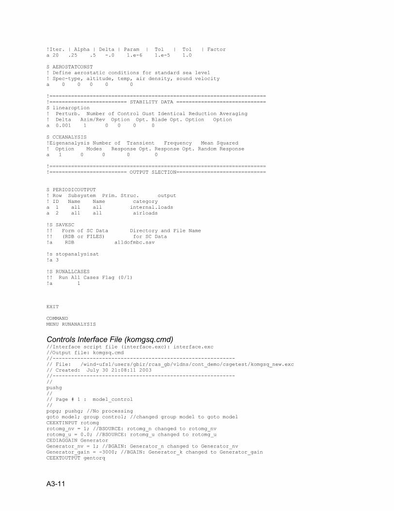
A3-11

!Iter. | Alpha | Delta | Param | Tol | Tol | Factor a 20 .25 .5 -.0 1.e-6 1.e-5 1.0 S AEROSTATCONST ! Define aerostatic conditions for standard sea level ! Spec-type, altitude, temp, air density, sound velocity a 0 0 0 0 0 !====================================================================== !========================= STABILITY DATA ============================= S linearoption ! Perturb. Number of Control Gust Identical Reduction Averaging ! Delta Azim/Rev Option Opt. Blade Opt. Option Option a 0.001 1 0 0 0 0 S CCEANALYSIS !Eigenanalysis Number of Transient Frequency Mean Squared ! Option Modes Response Opt. Response Opt. Random Response a 1 0 0 0 0 !====================================================================== !========================= OUTPUT SLECTION============================= S PERIODICOUTPUT ! Row Subsystem Prim. Struc. output ! ID Name Name category a 1 all all internal.loads a 2 all all airloads !S SAVESC !! Form of SC Data Directory and File Name !! (RDB or FILES) for SC Data !a RDB alldofmbc.sav !s stopanalysisat !a 3 !S RUNALLCASES !! Run All Cases Flag (0/1) !a 1 EXIT COMMAND MENU RUNANALYSIS

Controls Interface File (komgsq.cmd) //Interface script file (interface.exc): interface.exc //Output file: komgsq.cmd //----------------------------------------------------------- // File: /wind-ufs1/users/gbir/rcas_gb/vldns/cont_demo/csgetest/komgsq_new.exc // Created: July 30 21:08:11 2003 //----------------------------------------------------------- // pushg // // Page # 1 : model_control // popg; pushg; //No processing goto model; group control; //changed group model to goto model CEEXTINPUT rotomg rotomg_nv = 1; //BSOURCE: rotomg_n changed to rotomg_nv rotomg_u = 0.0; //BSOURCE: rotomg_u changed to rotomg_u CEDIAGGAIN Generator Generator_nv = 1; //BGAIN: Generator_n changed to Generator_nv Generator_gain = -3000; //BGAIN: Generator_k changed to Generator_gain CEEXTOUTPUT gentorq

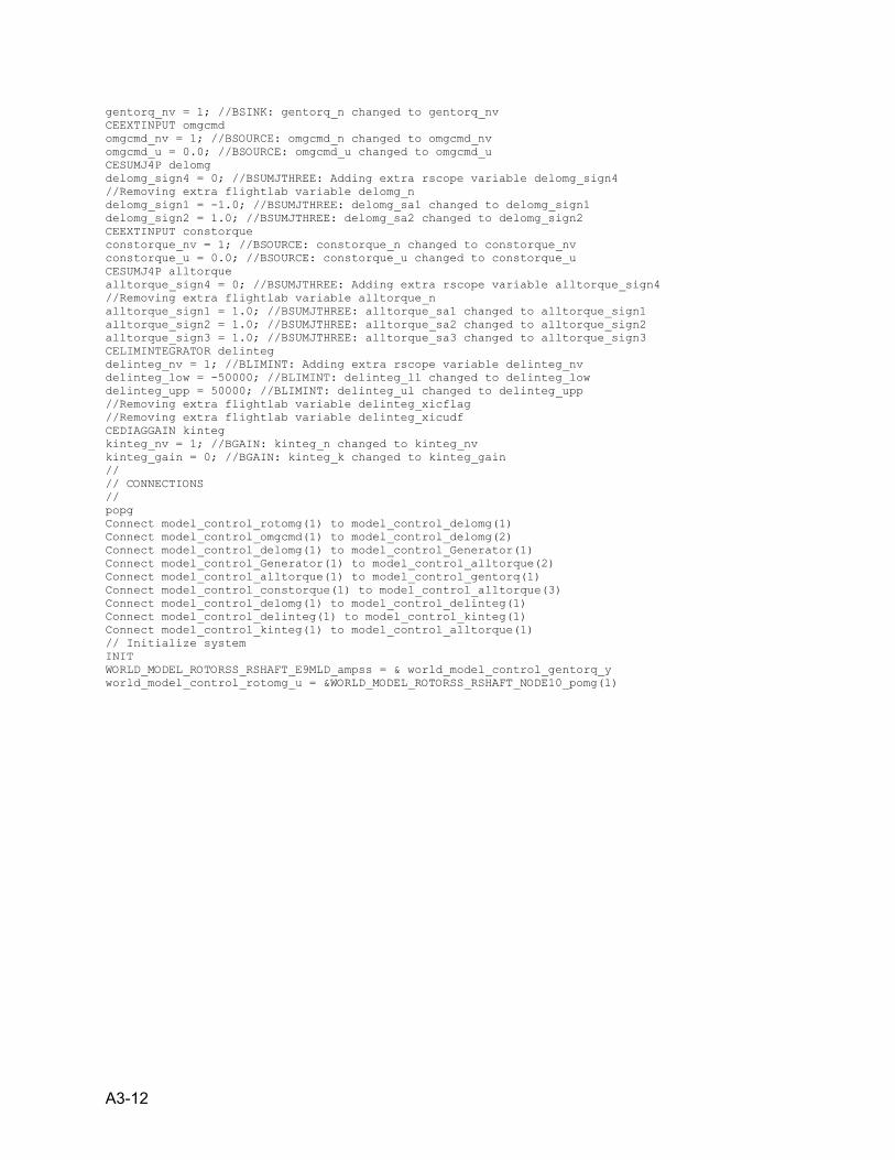
A3-12

gentorq_nv = 1; //BSINK: gentorq_n changed to gentorq_nv CEEXTINPUT omgcmd omgcmd_nv = 1; //BSOURCE: omgcmd_n changed to omgcmd_nv omgcmd_u = 0.0; //BSOURCE: omgcmd_u changed to omgcmd_u CESUMJ4P delomg delomg_sign4 = 0; //BSUMJTHREE: Adding extra rscope variable delomg_sign4 //Removing extra flightlab variable delomg_n delomg_sign1 = -1.0; //BSUMJTHREE: delomg_sa1 changed to delomg_sign1 delomg_sign2 = 1.0; //BSUMJTHREE: delomg_sa2 changed to delomg_sign2 CEEXTINPUT constorque constorque_nv = 1; //BSOURCE: constorque_n changed to constorque_nv constorque_u = 0.0; //BSOURCE: constorque_u changed to constorque_u CESUMJ4P alltorque alltorque_sign4 = 0; //BSUMJTHREE: Adding extra rscope variable alltorque_sign4 //Removing extra flightlab variable alltorque_n alltorque_sign1 = 1.0; //BSUMJTHREE: alltorque_sa1 changed to alltorque_sign1 alltorque_sign2 = 1.0; //BSUMJTHREE: alltorque_sa2 changed to alltorque_sign2 alltorque_sign3 = 1.0; //BSUMJTHREE: alltorque_sa3 changed to alltorque_sign3 CELIMINTEGRATOR delinteg delinteg_nv = 1; //BLIMINT: Adding extra rscope variable delinteg_nv delinteg_low = -50000; //BLIMINT: delinteg_ll changed to delinteg_low delinteg_upp = 50000; //BLIMINT: delinteg_ul changed to delinteg_upp //Removing extra flightlab variable delinteg_xicflag //Removing extra flightlab variable delinteg_xicudf CEDIAGGAIN kinteg kinteg_nv = 1; //BGAIN: kinteg_n changed to kinteg_nv kinteg_gain = 0; //BGAIN: kinteg_k changed to kinteg_gain // // CONNECTIONS // popg Connect model_control_rotomg(1) to model_control_delomg(1) Connect model_control_omgcmd(1) to model_control_delomg(2) Connect model_control_delomg(1) to model_control_Generator(1) Connect model_control_Generator(1) to model_control_alltorque(2) Connect model_control_alltorque(1) to model_control_gentorq(1) Connect model_control_constorque(1) to model_control_alltorque(3) Connect model_control_delomg(1) to model_control_delinteg(1) Connect model_control_delinteg(1) to model_control_kinteg(1) Connect model_control_kinteg(1) to model_control_alltorque(1) // Initialize system INIT WORLD_MODEL_ROTORSS_RSHAFT_E9MLD_ampss = & world_model_control_gentorq_y world_model_control_rotomg_u = &WORLD_MODEL_ROTORSS_RSHAFT_NODE10_pomg(1)

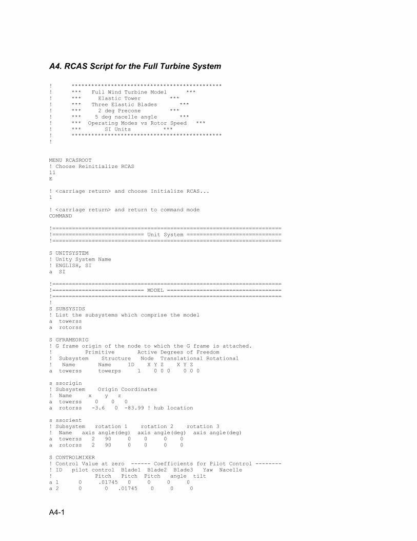
A4-1

A4. RCAS Script for the Full Turbine System ! ********************************************** ! *** Full Wind Turbine Model *** ! *** Elastic Tower *** ! *** Three Elastic Blades *** ! *** 2 deg Precone *** ! *** 5 deg nacelle angle *** ! *** Operating Modes vs Rotor Speed *** ! *** SI Units *** ! ********************************************** ! MENU RCASROOT ! Choose Reinitialize RCAS 11 E ! <carriage return> and choose Initialize RCAS... 1 ! <carriage return> and return to command mode COMMAND !====================================================================== !============================ Unit System ============================= !====================================================================== S UNITSYSTEM ! Unity System Name ! ENGLISH, SI a SI !====================================================================== !============================ MODEL =================================== !====================================================================== ! S SUBSYSIDS ! List the subsystems which comprise the model a towerss a rotorss S GFRAMEORIG ! G frame origin of the node to which the G frame is attached. ! Primitive Active Degrees of Freedom ! Subsystem Structure Node Translational Rotational ! Name Name ID X Y Z X Y Z a towerss towerps 1 0 0 0 0 0 0 s ssorigin ! Subsystem Origin Coordinates ! Name x y z a towerss 0 0 0 a rotorss -3.6 0 -83.99 ! hub location s ssorient ! Subsystem rotation 1 rotation 2 rotation 3 ! Name axis angle(deg) axis angle(deg) axis angle(deg) a towerss 2 90 0 0 0 0 a rotorss 2 90 0 0 0 0 S CONTROLMIXER ! Control Value at zero ------ Coefficients for Pilot Control -------- ! ID pilot control Blade1 Blade2 Blade3 Yaw Nacelle ! Pitch Pitch Pitch angle tilt a 1 0 .01745 0 0 0 0 a 2 0 0 .01745 0 0 0

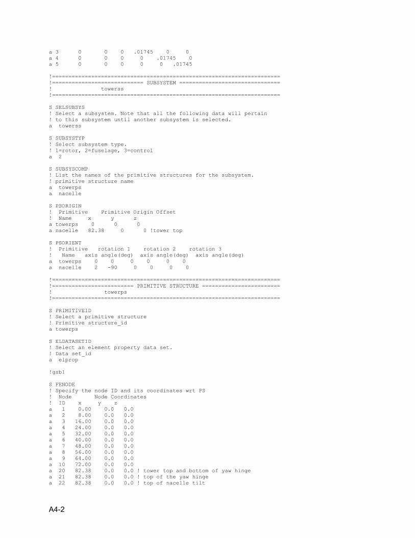
A4-2

a 3 0 0 0 .01745 0 0 a 4 0 0 0 0 .01745 0 a 5 0 0 0 0 0 .01745 !====================================================================== !============================ SUBSYSTEM =============================== ! towerss !====================================================================== S SELSUBSYS ! Select a subsystem. Note that all the following data will pertain ! to this subsystem until another subsystem is selected. a towerss S SUBSYSTYP ! Select subsystem type. ! 1=rotor, 2=fuselage, 3=control a 2 S SUBSYSCOMP ! List the names of the primitive structures for the subsystem. ! primitive structure name a towerps a nacelle S PSORIGIN ! Primitive Primitive Origin Offset ! Name x y z a towerps 0 0 0 a nacelle 82.38 0 0 !tower top S PSORIENT ! Primitive rotation 1 rotation 2 rotation 3 ! Name axis angle(deg) axis angle(deg) axis angle(deg) a towerps 0 0 0 0 0 0 a nacelle 2 -90 0 0 0 0 !====================================================================== !========================= PRIMITIVE STRUCTURE ======================== ! towerps !====================================================================== S PRIMITIVEID ! Select a primitive structure ! Primitive structure_id a towerps S ELDATASETID ! Select an element property data set. ! Data set_id a elprop !gsb1 S FENODE ! Specify the node ID and its coordinates wrt PS ! Node Node Coordinates ! ID x y z a 1 0.00 0.0 0.0 a 2 8.00 0.0 0.0 a 3 16.00 0.0 0.0 a 4 24.00 0.0 0.0 a 5 32.00 0.0 0.0 a 6 40.00 0.0 0.0 a 7 48.00 0.0 0.0 a 8 56.00 0.0 0.0 a 9 64.00 0.0 0.0 a 10 72.00 0.0 0.0 a 20 82.38 0.0 0.0 ! tower top and bottom of yaw hinge a 21 82.38 0.0 0.0 ! top of the yaw hinge a 22 82.38 0.0 0.0 ! top of nacelle tilt

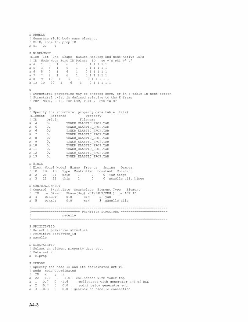
A4-3

S RBMELE ! Generate rigid body mass element. ! ELID, node ID, prop ID A 51 22 1 S NLBEAMDEF !Elem 1st 2nd Shape NGauss MatProp End Node Active DOFs ! ID Node Node Func ID Points ID ue v w phi w' v' a 4 1 3 1 6 1 0 1 1 1 1 1 a 5 3 5 1 6 1 0 1 1 1 1 1 a 6 5 7 1 6 1 0 1 1 1 1 1 a 7 7 9 1 6 1 0 1 1 1 1 1 a 8 9 10 1 6 1 0 1 1 1 1 1 a 13 10 20 1 6 1 0 1 1 1 1 1 N ! Structural properties may be entered here, or in a table in next screen ! Structural twist is defined relative to the E frame ! PRP-INDEX, ELID, PRP-LOC, PRPID, STR-TWIST N ! Specify the structural property data table (file) !Element Refernce Property ! ID origin Filename A 4 0. TOWER_ELASTIC_PROP.TAB A 5 0. TOWER_ELASTIC_PROP.TAB A 6 0. TOWER_ELASTIC_PROP.TAB A 7 0. TOWER_ELASTIC_PROP.TAB A 8 0. TOWER_ELASTIC_PROP.TAB A 9 0. TOWER_ELASTIC_PROP.TAB A 10 0. TOWER_ELASTIC_PROP.TAB A 11 0. TOWER_ELASTIC_PROP.TAB A 12 0. TOWER_ELASTIC_PROP.TAB A 13 0. TOWER_ELASTIC_PROP.TAB S HINGE ! Elem. Node1 Node2 Hinge Free or Spring Damper ! ID ID ID Type Controlled Constant Constant a 2 20 21 xhin 1 0 0 !Yaw hinge a 3 21 22 yhin 1 0 0 !ncaelle tilt hinge S CONTROLCONNECT ! Control Swashplate Swashplate Element Type Element ! ID or Direct Phase(deg) (HIN/AUX/ENG ) or ACP ID a 4 DIRECT 0.0 HIN 2 !yaw a 5 DIRECT 0.0 HIN 3 !Nacelle tilt !====================================================================== !========================= PRIMITIVE STRUCTURE ======================== ! nacelle !====================================================================== S PRIMITIVEID ! Select a primitive structure ! Primitive structure_id a nacelle S ELDATASETID ! Select an element property data set. ! Data set_id a elprop S FENODE ! Specify the node ID and its coordinates wrt PS ! Node Node Coordinates ! ID x y z a 22 0.0 0 0.0 ! collocated with tower top a 1 0.7 0 -1.6 ! collocated with generator end of HSS a 2 0.7 0 0.0 ! point below generator end a 3 -0.3 0 0.0 ! gearbox to nacelle connection

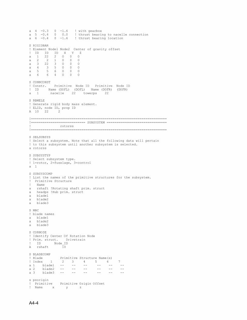
A4-4

a 4 -0.3 0 -1.6 ! with gearbox a 5 -0.4 0 0.0 ! thrust bearing to nacelle connection a 6 -0.4 0 -1.6 ! thrust bearing location S RIGIDBAR ! Element Node1 Node2 Center of gravity offset ! ID ID ID X Y Z a 1 22 2 0 0 0 a 2 2 1 0 0 0 a 3 22 3 0 0 0 a 4 3 5 0 0 0 a 5 5 6 0 0 0 a 6 6 4 0 0 0 S CONNCONST ! Constr. Primitive Node ID Primitive Node ID ! ID Name (DOFL) (DOFL) Name (DOFR) (DOFR) a 1 nacelle 22 towerps 22 S RBMELE ! Generate rigid body mass element. ! ELID, node ID, prop ID A 10 22 2 !====================================================================== !============================ SUBSYSTEM =============================== ! rotorss !====================================================================== S SELSUBSYS ! Select a subsystem. Note that all the following data will pertain ! to this subsystem until another subsystem is selected. a rotorss S SUBSYSTYP ! Select subsystem type. ! 1=rotor, 2=fuselage, 3=control a 1 S SUBSYSCOMP ! List the names of the primitive structures for the subsystem. ! Primitive Structure ! Name a rshaft !Rotating shaft prim. struct a headps !Hub prim. struct a blade1 a blade2 a blade3 S MBC ! blade names a blade1 a blade2 a blade3 S CORNODE ! Identify Center Of Rotation Node ! Prim. struct. Drivetrain ! ID Node_ID A rshaft 10 S BLADECOMP ! Blade Primitive Structure Name(s) ! Index 1 2 3 4 5 6 7 a 1 blade1 -- -- -- -- -- -- a 2 blade2 -- -- -- -- -- -- a 3 blade3 -- -- -- -- -- -- s psorigin ! Primitive Primitive Origin Offset ! Name x y z

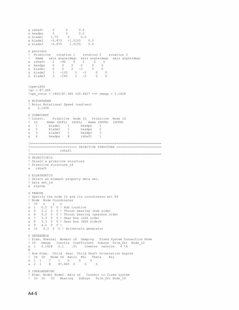
A4-5

a rshaft 0 0 0.0 a headps 0 0 0.0 a blade1 1.75 0 0.0 a blade2 -0.875 -1.5155 0.0 a blade3 -0.875 1.5155 0.0 s psorient ! Primitive rotation 1 rotation 2 rotation 3 ! Name axis angle(deg) axis angle(deg) axis angle(deg) a rshaft 2 -90 0 0 0 0 a headps 0 0 0 0 0 0 a blade1 0 0 2 -2 0 0 a blade2 3 -120 2 -2 0 0 a blade3 3 -240 2 -2 0 0 !rpm=1800 !gr = 87.965 !rpm_rotor = 1800/87.965 =20.4627 ==> omega = 2.1428 S ROTORPARAM ! Rotor Rotational Speed (rad/sec) a 2.1428 S CONNCONST ! Constr. Primitive Node ID Primitive Node ID ! ID Name (DOFL) (DOFL) Name (DOFR) (DOFR) a 1 blade1 1 headps 1 a 2 blade2 1 headps 2 a 3 blade3 1 headps 3 a 4 headps 8 rshaft 1 !====================================================================== !========================= PRIMITIVE STRUCTURE ======================== ! rshaft !====================================================================== S PRIMITIVEID ! Select a primitive structure ! Primitive structure_id a rshaft S ELDATASETID ! Select an element property data set. ! Data set_id a elprop S FENODE ! Specify the node ID and its coordinates wrt PS ! Node Node Coordinates ! ID x y z a 1 0.0 0 0 ! Hub location a 5 3.2 0 0 ! Thrust bearing (hub side) a 6 3.2 0 0 ! Thrust bearing (gearbox side) a 7 3.3 0 0 ! Gear box (LSS side) a 8 3.3 0 0 ! Gear box (HSS side)B a 9 4.2 0 0 ! a 10 4.3 0 0 ! drivetrain generator S SEGEARBOX ! Elem. Nominal Moment of Damping Fixed System Connection Node ! ID Omega Inertia Coefficient Subsys Prim_Str Node_ID a 1 2.1428 2.1 .01 towerss nacelle 4 !A N ! Row Elem. Child Gear Child Shaft Orientation Angles ! ID ID Node ID Ratio Phi Theta Psi a 1 1 7 1 0 0 0 a 2 1 8 87.965 0 0 0 S IDEALBEARING ! Elem. Node1 Node2 Axis of Connect to fixed system ! ID ID ID Bearing Subsys Prim_Str Node_ID

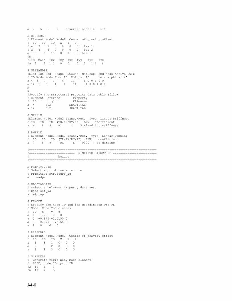
A4-6

a 2 5 6 X towerss nacelle 6 !E S RIGIDBAR ! Element Node1 Node2 Center of gravity offset ! ID ID ID X Y Z !!a 3 1 5 0 0 0 ! lss 1 !!a 4 6 7 0 0 0 ! lss 2 a 5 9 10 0 0 0 ! hss 1 !N ! ID Mass Ixx Ixy Ixz Iyy Iyz Izz !a 3 .2 1.1 0 0 0 0 1.1 !? S NLBEAMDEF !Elem 1st 2nd Shape NGauss MatProp End Node Active DOFs ! ID Node Node Func ID Points ID ue v w phi w' v' a 4 6 7 1 6 11 1 0 0 1 0 0 a 14 1 5 1 6 11 1 0 0 1 0 0 N N !Specify the structural property data table (file) ! Element Refernce Property ! ID origin Filename a 4 3.2 SHAFT.TAB a 14 3.2 SHAFT.TAB S SPRELE !Element Node1 Node2 Trans./Rot. Type Linear stiffness ! ID ID ID (TR/RX/RY/RZ) (L/N) coefficient a 6 8 9 RX L 3.62E+6 !dt stiffness S DMPELE ! Element Node1 Node2 Trans./Rot. Type Linear Damping ! ID ID ID (TR/RX/RY/RZ) (L/N) coefficient a 7 8 9 RX L 0000 ! dt damping !====================================================================== !========================= PRIMITIVE STRUCTURE ======================== ! headps !====================================================================== S PRIMITIVEID ! Select a primitive structure ! Primitive structure_id a headps S ELDATASETID ! Select an element property data set. ! Data set_id a elprop S FENODE ! Specify the node ID and its coordinates wrt PS ! Node Node Coordinates ! ID x y z a 1 1.75 0 0 a 2 -0.875 -1.5155 0 a 3 -0.875 1.5155 0 a 8 0 0 0 S RIGIDBAR ! Element Node1 Node2 Center of gravity offset ! ID ID ID X Y Z a 1 8 1 0 0 0 a 2 8 2 0 0 0 a 3 8 3 0 0 0 ! S RBMELE !! Generate rigid body mass element. !! ELID, node ID, prop ID !A 11 1 3 !A 12 2 3

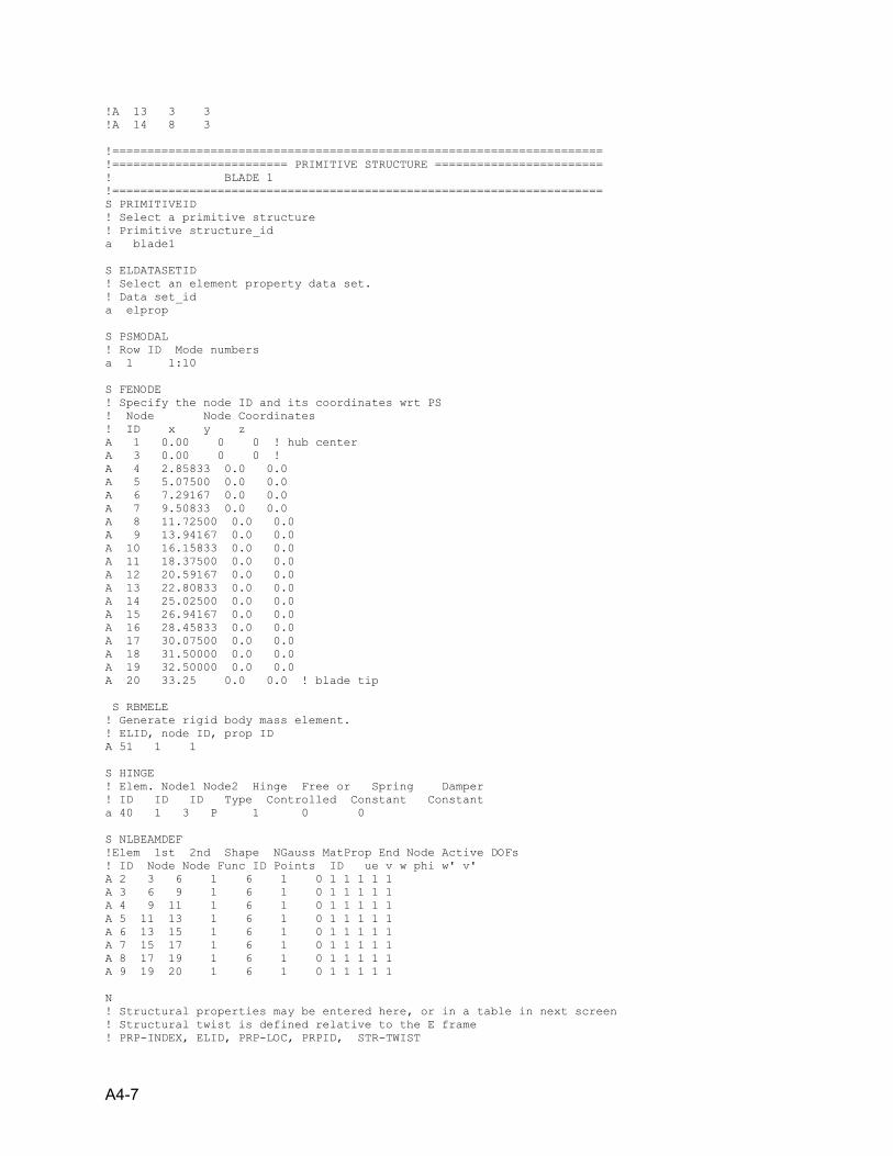
A4-7

!A 13 3 3 !A 14 8 3 !====================================================================== !========================= PRIMITIVE STRUCTURE ======================== ! BLADE 1 !====================================================================== S PRIMITIVEID ! Select a primitive structure ! Primitive structure_id a blade1 S ELDATASETID ! Select an element property data set. ! Data set_id a elprop S PSMODAL ! Row ID Mode numbers a 1 1:10 S FENODE ! Specify the node ID and its coordinates wrt PS ! Node Node Coordinates ! ID x y z A 1 0.00 0 0 ! hub center A 3 0.00 0 0 ! A 4 2.85833 0.0 0.0 A 5 5.07500 0.0 0.0 A 6 7.29167 0.0 0.0 A 7 9.50833 0.0 0.0 A 8 11.72500 0.0 0.0 A 9 13.94167 0.0 0.0 A 10 16.15833 0.0 0.0 A 11 18.37500 0.0 0.0 A 12 20.59167 0.0 0.0 A 13 22.80833 0.0 0.0 A 14 25.02500 0.0 0.0 A 15 26.94167 0.0 0.0 A 16 28.45833 0.0 0.0 A 17 30.07500 0.0 0.0 A 18 31.50000 0.0 0.0 A 19 32.50000 0.0 0.0 A 20 33.25 0.0 0.0 ! blade tip S RBMELE ! Generate rigid body mass element. ! ELID, node ID, prop ID A 51 1 1 S HINGE ! Elem. Node1 Node2 Hinge Free or Spring Damper ! ID ID ID Type Controlled Constant Constant a 40 1 3 P 1 0 0 S NLBEAMDEF !Elem 1st 2nd Shape NGauss MatProp End Node Active DOFs ! ID Node Node Func ID Points ID ue v w phi w' v' A 2 3 6 1 6 1 0 1 1 1 1 1 A 3 6 9 1 6 1 0 1 1 1 1 1 A 4 9 11 1 6 1 0 1 1 1 1 1 A 5 11 13 1 6 1 0 1 1 1 1 1 A 6 13 15 1 6 1 0 1 1 1 1 1 A 7 15 17 1 6 1 0 1 1 1 1 1 A 8 17 19 1 6 1 0 1 1 1 1 1 A 9 19 20 1 6 1 0 1 1 1 1 1 N ! Structural properties may be entered here, or in a table in next screen ! Structural twist is defined relative to the E frame ! PRP-INDEX, ELID, PRP-LOC, PRPID, STR-TWIST

A4-8

N S NLBEAMDEF !Elem 1st 2nd Shape NGauss MatProp End Node Active DOFs ! ID Node Node Func ID Points ID ue v w phi w' v' A 2 3 6 1 6 1 0 1 1 1 1 1 A 3 6 9 1 6 1 0 1 1 1 1 1 A 4 9 11 1 6 1 0 1 1 1 1 1 A 5 11 13 1 6 1 0 1 1 1 1 1 A 6 13 15 1 6 1 0 1 1 1 1 1 A 7 15 17 1 6 1 0 1 1 1 1 1 A 8 17 19 1 6 1 0 1 1 1 1 1 A 9 19 20 1 6 1 1 0 0 0 0 0 S CONTROLCONNECT ! Control Swashplate Swashplate Element Type Element ! ID or Direct Phase(deg) (HIN/AUX/ENG ...) or ACP ID a 1 DIRECT 0.0 HIN 40 !====================================================================== !========================= Copy Primitives =========================== !====================================================================== S PRIMIT ! Copy ID, source PS, destination PS a 1 blade1 blade2 a 2 blade2 blade3 EXIT COMMAND copyprimstruct COMMAND !====================================================================== !===================== Correct control connections ==================== ! for the other blades !====================================================================== S PRIMITIVEID !! Select a primitive structure !! Primitive structure_id c blade2 ! S CONTROLCONNECT !! Control Swashplate Swashplate Element Type Element !! ID or Direct Phase(deg) (HIN/AUX/ENG ...) or ACP ID d 1 a 2 DIRECT 0.0 HIN 40 ! S PRIMITIVEID !! Select a primitive structure !! Primitive structure_id c blade3 ! S CONTROLCONNECT !! Control Swashplate Swashplate Element Type Element !! ID or Direct Phase(deg) (HIN/AUX/ENG ...) or ACP ID d 1 a 3 DIRECT 0.0 HIN 40 !====================================================================== !============== Rotating to Nonrotating Connection ==================== !====================================================================== S ROTNONCONST !Cnstr. Subsys. Primit. Node Subsys. Primit. Node ! ID Name Name ID Name Name ID a 1 towerss nacelle 1 rotorss rshaft 10

A4-9

!====================================================================== !======================== STRUCTURAL PROPERTIES ======================= ! ELPROP !====================================================================== S ELEPROPID ! Add the name of an element property data set. ! element_prop_id a elprop S RBMPRP ! Prop Elem. Center Mass Offset --- Mass Moment of Inertia Matrix --- ! ID Mass X Y Z Ixx, Ixy Ixz Iyy Iyz Izz A 1 1.e-7 0 0 0 0 0 0 0 0 0 A 2 51170 -0.1251 0 1.3722 0 0 0 55946.8 0 48329.2 A 3 15148 0 0 0 0 0 0 0 0 0 S NLBSHAPE ! NLB Shape Function ----- Shape Function Orders ---- ! Set ID Axial Bending Torsion A 1 1 0 1 !====================================================================== !====================================================================== ! END OF MODEL DEFINITION !====================================================================== !====================================================================== !====================================================================== !========================== ANALYSIS DATA ============================= !====================================================================== S SELANALYSIS ! Case ID Trim Mane Stab Init ----- Scope Script ----- ! (0:3) (0:4) (0:1) Cond File Name a 01 0 0 1 S NO a 02 0 0 1 S NO a 03 0 0 1 S NO a 04 0 0 1 S NO a 05 0 0 1 S NO a 06 0 0 1 S NO a 07 0 0 1 S NO a 08 0 0 1 S NO a 09 0 0 1 S NO a 10 0 0 1 S NO a 11 0 0 1 S NO a 12 0 0 1 S NO a 13 0 0 1 S NO a 14 0 0 1 S NO a 15 0 0 1 S NO a 16 0 0 1 S NO a 17 0 0 1 S NO a 18 0 0 1 S NO a 19 0 0 1 S NO a 20 0 0 1 S NO a 21 0 0 1 S NO a 22 0 0 1 S NO a 23 0 0 1 S NO N ! Case ID Case Title (Maximum 30 Characters) a 01 case01 a 02 case02 a 03 case03 a 04 case04 a 05 case05 a 06 case06 a 07 case07 a 08 case08 a 09 case09 a 10 case10

A4-10

a 11 case11 a 12 case12 a 13 case13 a 14 case14 a 15 case15 a 16 case16 a 17 case17 a 18 case18 a 19 case19 a 20 case20 a 21 case21 a 22 case22 a 23 case23 N ! Case_Var --Screen Name-- Data_Group Screen Field Row ! ID ("--" if none) Number Number Number a OMEGA ROTORPARAM ROTORSS 1 1 1 N !Row id Case_Var_ID Case ID Value a 1 OMEGA 01 .01 a 2 OMEGA 02 .5 a 3 OMEGA 03 1. a 4 OMEGA 04 02 a 5 OMEGA 05 04 a 6 OMEGA 06 06 a 7 OMEGA 07 08 a 8 OMEGA 08 10 a 9 OMEGA 09 12 a 10 OMEGA 10 14 a 11 OMEGA 11 16 a 12 OMEGA 12 18 a 13 OMEGA 13 20 a 14 OMEGA 14 22 a 15 OMEGA 15 24 a 16 OMEGA 16 26 a 17 OMEGA 17 28 a 18 OMEGA 18 30 a 19 OMEGA 19 32 a 20 OMEGA 20 34 a 21 OMEGA 21 36 a 22 OMEGA 22 38 a 23 OMEGA 23 40 S INITCOND ! Initial Controls ! Blade1 Blade2 Blade3 Yaw Nacelle ! Pitch Pitch Pitch angle tilt a -2.6 -2.6 -2.6 0 -5 N ! G frame position Frame wrt I ! X Y Z Roll Pitch Yaw a 0 0 0 0 0 0 S SYSTEMFLAGS ! Global element formulation flags (1=Yes, 0=No) ! Gravity Aero ! Effects Effects a 0 0 S CONVERGETOL ! # of # of # of Displ. Tolerance veloc tolerance Min. ! Trim PSol Time (Trans, Rot) (Trans, Rot) # of ! Iter Iter Step (ft) (rad) (ft/sec)(rad/sec) PS Rev a 10 4 36 0.005 0.01 1.0 0.01 5 SCREEN INTEGPARAM !No. of| Newmark Constants| HHT | Displace. | Velocity | Relax. !Iter. | Alpha | Delta | Param | Tol | Tol | Factor

A4-11

a 20 .25 .5 -.0 1.e-6 1.e-5 1.0 S AEROSTATCONST ! Define aerostatic conditions for standard sea level ! Spec-type, altitude, temp, air density, sound velocity a 0 0 0 0 0 !====================================================================== !========================= STABILITY DATA ============================= S linearoption ! Perturb. Number of Control Gust Identical Reduction Averaging ! Delta Azim/Rev Option Opt. Blade Opt. Option Option a 0.001 1 0 0 0 0 S CCEANALYSIS !Eigenanalysis Number of Transient Frequency Mean Squared ! Option Modes Response Opt. Response Opt. Random Response a 1 0 0 0 0 !====================================================================== !========================= OUTPUT SLECTION============================= S PERIODICOUTPUT ! Row Subsystem Prim. Struc. output ! ID Name Name category a 1 all all internal.loads a 2 all all airloads S SAVESC ! Form of SC Data Directory and File Name ! (RDB or FILES) for SC Data a RDB 10bmodmbc.sav !s stopanalysisat !a 3 S RUNALLCASES ! Run All Cases Flag (0/1) a 1 EXIT COMMAND MENU RUNANALYSIS

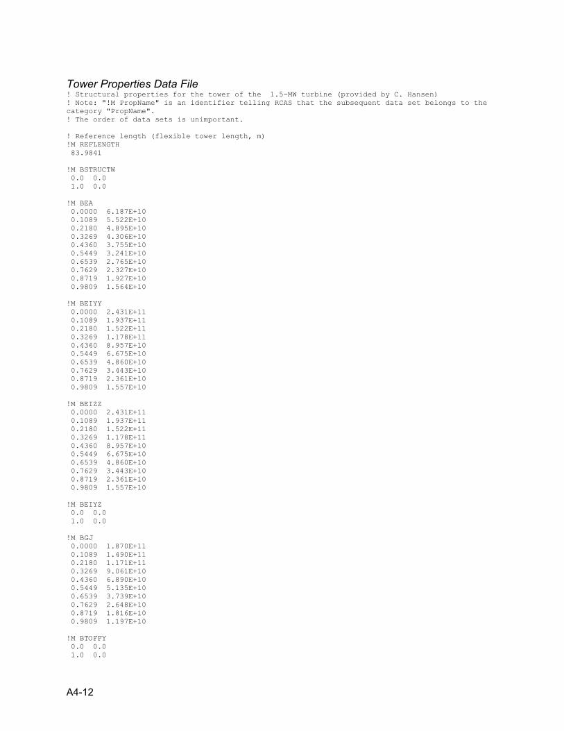
A4-12

Tower Properties Data File ! Structural properties for the tower of the 1.5-MW turbine (provided by C. Hansen) ! Note: "!M PropName" is an identifier telling RCAS that the subsequent data set belongs to the category "PropName". ! The order of data sets is unimportant. ! Reference length (flexible tower length, m) !M REFLENGTH 83.9841 !M BSTRUCTW 0.0 0.0 1.0 0.0 !M BEA 0.0000 6.187E+10 0.1089 5.522E+10 0.2180 4.895E+10 0.3269 4.306E+10 0.4360 3.755E+10 0.5449 3.241E+10 0.6539 2.765E+10 0.7629 2.327E+10 0.8719 1.927E+10 0.9809 1.564E+10 !M BEIYY 0.0000 2.431E+11 0.1089 1.937E+11 0.2180 1.522E+11 0.3269 1.178E+11 0.4360 8.957E+10 0.5449 6.675E+10 0.6539 4.860E+10 0.7629 3.443E+10 0.8719 2.361E+10 0.9809 1.557E+10 !M BEIZZ 0.0000 2.431E+11 0.1089 1.937E+11 0.2180 1.522E+11 0.3269 1.178E+11 0.4360 8.957E+10 0.5449 6.675E+10 0.6539 4.860E+10 0.7629 3.443E+10 0.8719 2.361E+10 0.9809 1.557E+10 !M BEIYZ 0.0 0.0 1.0 0.0 !M BGJ 0.0000 1.870E+11 0.1089 1.490E+11 0.2180 1.171E+11 0.3269 9.061E+10 0.4360 6.890E+10 0.5449 5.135E+10 0.6539 3.739E+10 0.7629 2.648E+10 0.8719 1.816E+10 0.9809 1.197E+10 !M BTOFFY 0.0 0.0 1.0 0.0

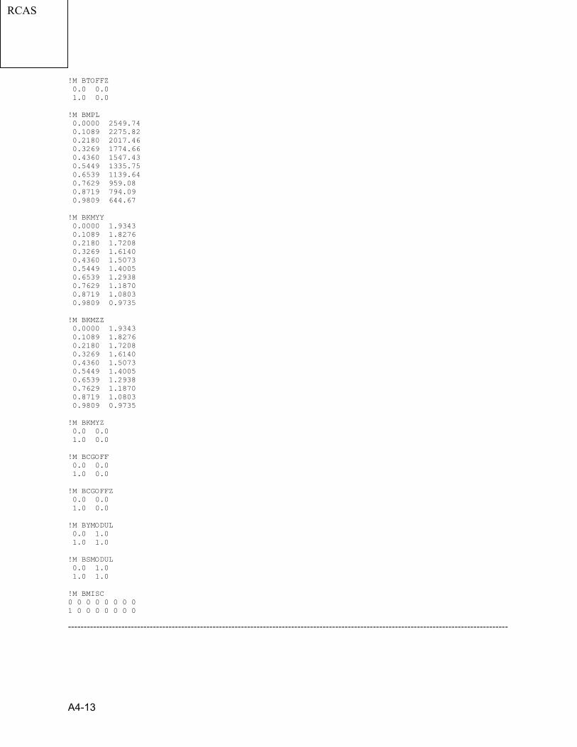
A4-13

!M BTOFFZ 0.0 0.0 1.0 0.0 !M BMPL 0.0000 2549.74 0.1089 2275.82 0.2180 2017.46 0.3269 1774.66 0.4360 1547.43 0.5449 1335.75 0.6539 1139.64 0.7629 959.08 0.8719 794.09 0.9809 644.67 !M BKMYY 0.0000 1.9343 0.1089 1.8276 0.2180 1.7208 0.3269 1.6140 0.4360 1.5073 0.5449 1.4005 0.6539 1.2938 0.7629 1.1870 0.8719 1.0803 0.9809 0.9735 !M BKMZZ 0.0000 1.9343 0.1089 1.8276 0.2180 1.7208 0.3269 1.6140 0.4360 1.5073 0.5449 1.4005 0.6539 1.2938 0.7629 1.1870 0.8719 1.0803 0.9809 0.9735 !M BKMYZ 0.0 0.0 1.0 0.0 !M BCGOFF 0.0 0.0 1.0 0.0 !M BCGOFFZ 0.0 0.0 1.0 0.0 !M BYMODUL 0.0 1.0 1.0 1.0 !M BSMODUL 0.0 1.0 1.0 1.0 !M BMISC 0 0 0 0 0 0 0 0 1 0 0 0 0 0 0 0

--------------------------------------------------------------------------------------------------------------------------------------------

RCAS

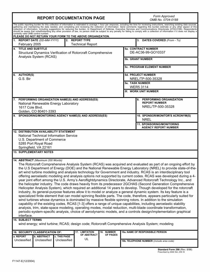
F1147-E(12/2004)

REPORT DOCUMENTATION PAGE Form Approved OMB No. 0704-0188

The public reporting burden for this collection of information is estimated to average 1 hour per response, including the time for reviewing instructions, searching existing data sources, gathering and maintaining the data needed, and completing and reviewing the collection of information. Send comments regarding this burden estimate or any other aspect of this collection of information, including suggestions for reducing the burden, to Department of Defense, Executive Services and Communications Directorate (0704-0188). Respondents should be aware that notwithstanding any other provision of law, no person shall be subject to any penalty for failing to comply with a collection of information if it does not display a currently valid OMB control number. PLEASE DO NOT RETURN YOUR FORM TO THE ABOVE ORGANIZATION. 1. REPORT DATE (DD-MM-YYYY)

February 2005 2. REPORT TYPE

Technical Report 3. DATES COVERED (From - To)

5a. CONTRACT NUMBER

DE-AC36-99-GO10337

5b. GRANT NUMBER

4. TITLE AND SUBTITLE Structural Dynamics Verification of Rotorcraft Comprehensive Analysis System (RCAS)

5c. PROGRAM ELEMENT NUMBER

5d. PROJECT NUMBER NREL/TP-500-35328

5e. TASK NUMBER WER5 3114

6. AUTHOR(S) G.S. Bir

5f. WORK UNIT NUMBER

7. PERFORMING ORGANIZATION NAME(S) AND ADDRESS(ES) National Renewable Energy Laboratory 1617 Cole Blvd. Golden, CO 80401-3393

8. PERFORMING ORGANIZATION REPORT NUMBER NREL/TP-500-35328

10. SPONSOR/MONITOR'S ACRONYM(S) NREL

9. SPONSORING/MONITORING AGENCY NAME(S) AND ADDRESS(ES)

11. SPONSORING/MONITORING AGENCY REPORT NUMBER

12. DISTRIBUTION AVAILABILITY STATEMENT National Technical Information Service U.S. Department of Commerce 5285 Port Royal Road Springfield, VA 22161

13. SUPPLEMENTARY NOTES

14. ABSTRACT (Maximum 200 Words) The Rotorcraft Comprehensive Analysis System (RCAS) was acquired and evaluated as part of an ongoing effort by the U.S Department of Energy (DOE) and the National Renewable Energy Laboratory (NREL) to provide state-of-the-art wind turbine modeling and analysis technology for Government and industry. RCAS is an interdisciplinary tool offering aeroelastic modeling and analysis options not supported by current codes. RCAS was developed during a 4-year joint effort among the U.S. Army’s Aeroflightdynamics Directorate, Advanced Rotorcraft Technology Inc., and the helicopter industry. The code draws heavily from its predecessor 2GCHAS (Second Generation Comprehensive Helicopter Analysis System), which required an additional 14 years to develop. Though developed for the rotorcraft industry, its general-purpose features allow it to model or analyze a general dynamic system. Its key feature is a specialized finite element that can model spinning flexible parts. The code, therefore, appears particularly suited for wind turbines whose dynamics is dominated by massive flexible spinning rotors. In addition to the simulation capability of the existing codes, RCAS [1-3] offers a range of unique capabilities, including aeroelastic stability analysis, trim, state-space modeling, operating modes, modal reduction, multi-blade coordinate transformation, periodic-system-specific analysis, choice of aerodynamic models, and a controls design/implementation graphical interface.

15. SUBJECT TERMS wind energy; wind turbine; RCAS; design code; Rotorcraft Comprehensive Analysis System; modeling

16. SECURITY CLASSIFICATION OF: 19a. NAME OF RESPONSIBLE PERSON a. REPORT

Unclassified b. ABSTRACT Unclassified

c. THIS PAGE Unclassified

17. LIMITATION OF ABSTRACT

UL

18. NUMBER OF PAGES

19b. TELEPHONE NUMBER (Include area code)

Standard Form 298 (Rev. 8/98) Prescribed by ANSI Std. Z39.18