professor of aeronautics & astronautics bifurcation buckling · pdf file ·...

MIT - 16.20 Fall, 2002

Unit 16 Bifurcation Buckling

Readings:Rivello 14.1, 14.2, 14.4

Paul A. Lagace, Ph.D.Professor of Aeronautics & Astronautics

and Engineering Systems

Paul A. Lagace © 2001

MIT - 16.20 Fall, 2002

V. Stability and Buckling

Paul A. Lagace © 2001 Unit 16 - 2

MIT - 16.20 Fall, 2002

Now consider the case of compressive loads and the instability they can cause. Consider only static instabilities (static loading as opposed to dynamic loading [e.g., flutter])

From Unified, defined instability via:

“A system becomes unstable when a negative stiffness overcomes the natural stiffness of the structure.”

(Physically, the more you push, it gives more and builds on itself)

Review some of the mathematical concepts. Limit initial discussions to columns.

Generally, there are two types of buckling/instability

• Bifurcation buckling • Snap-through buckling


MIT - 16.20 Fall, 2002

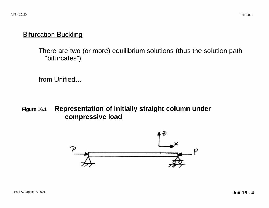
Bifurcation Buckling

There are two (or more) equilibrium solutions (thus the solution path “bifurcates”)

from Unified…

Figure 16.1 Representation of initially straight column under compressive load


MIT - 16.20 Fall, 2002

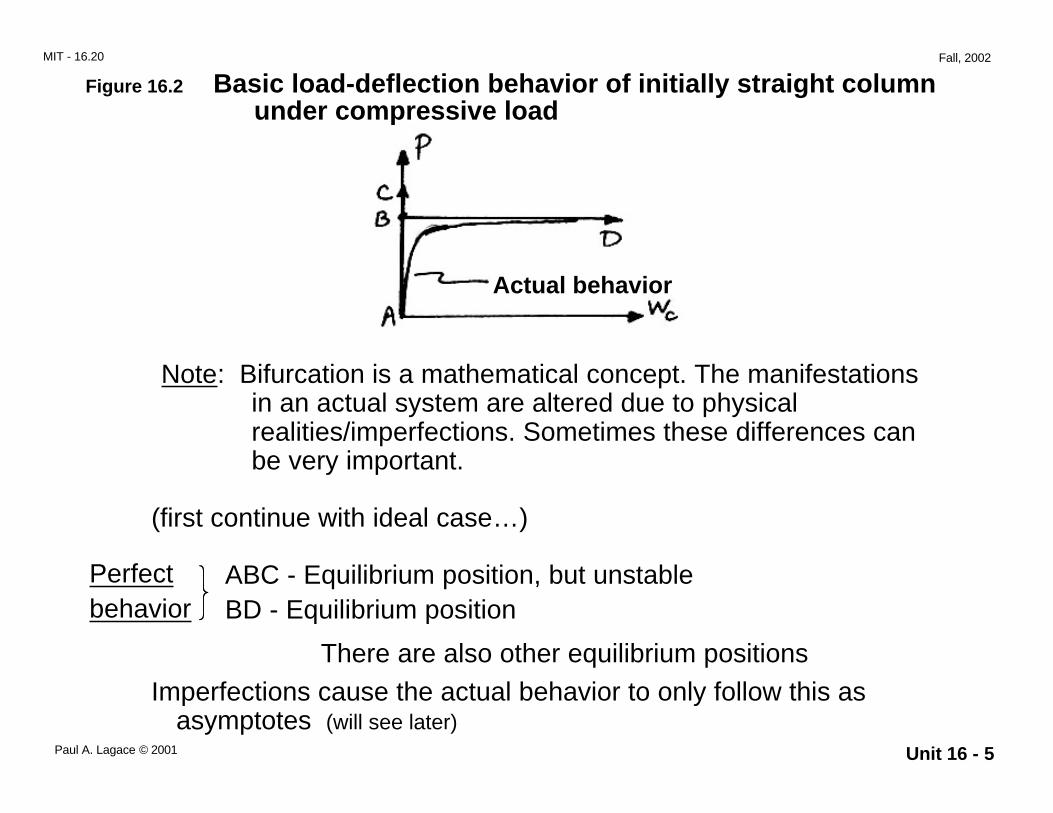
Figure 16.2 Basic load-deflection behavior of initially straight column under compressive load

Actual behavior

Note: Bifurcation is a mathematical concept. The manifestations in an actual system are altered due to physical realities/imperfections. Sometimes these differences can be very important.

(first continue with ideal case…)

Perfect ABC - Equilibrium position, but unstable behavior BD - Equilibrium position

There are also other equilibrium positions

Imperfections cause the actual behavior to only follow this as asymptotes (will see later)


MIT - 16.20 Fall, 2002

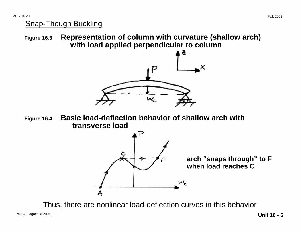
Snap-Though Buckling

Figure 16.3 Representation of column with curvature (shallow arch) with load applied perpendicular to column

Figure 16.4 Basic load-deflection behavior of shallow arch with transverse load

arch “snaps through” to F when load reaches C

Thus, there are nonlinear load-deflection curves in this behaviorPaul A. Lagace © 2001 Unit 16 - 6

MIT - 16.20 Fall, 2002

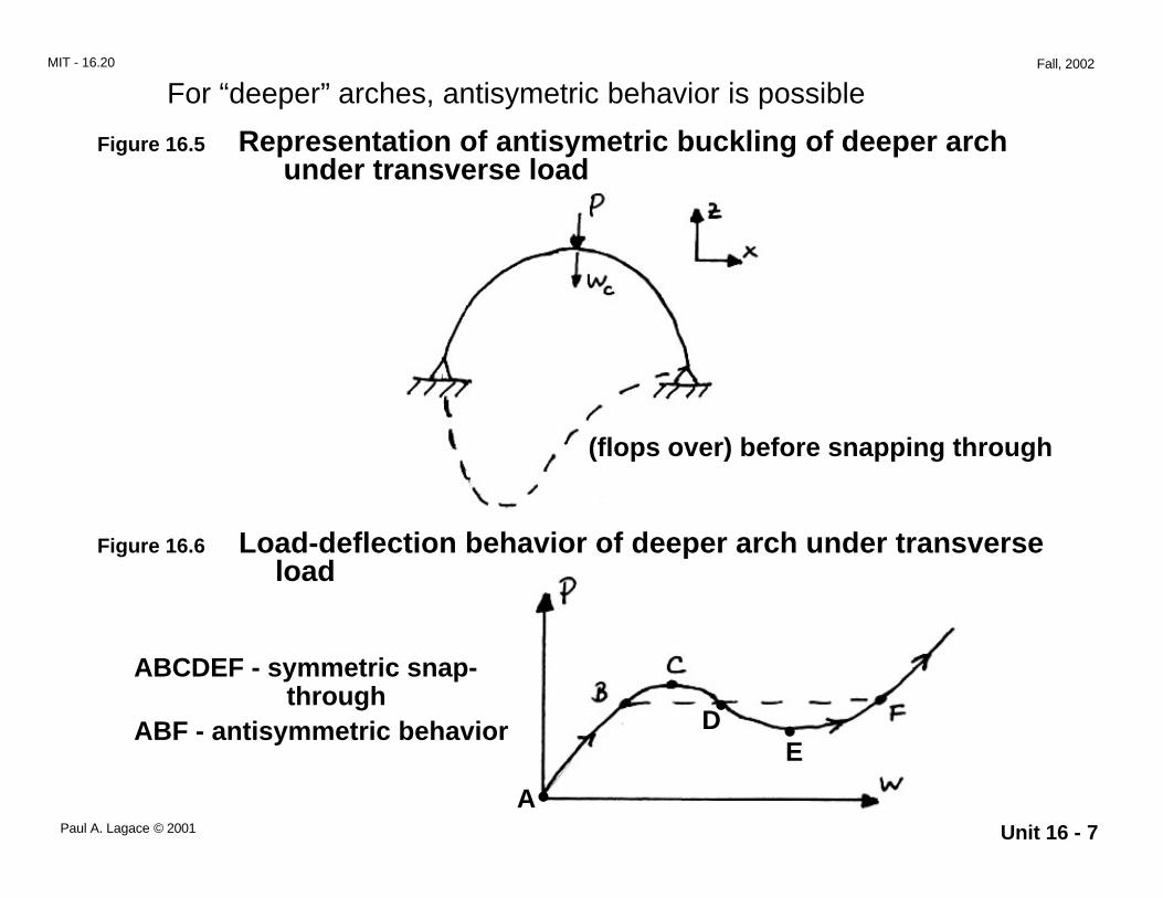
For “deeper” arches, antisymetric behavior is possible

Figure 16.5 Representation of antisymetric buckling of deeper arch under transverse load

(flops over) before snapping through

Figure 16.6 Load-deflection behavior of deeper arch under transverse load

ABCDEF - symmetric snap-through

ABF - antisymmetric behavior

A

D E

• •

• Paul A. Lagace © 2001 Unit 16 - 7

MIT - 16.20 Fall, 2002

Will deal mainly with…

Bifurcation Buckling

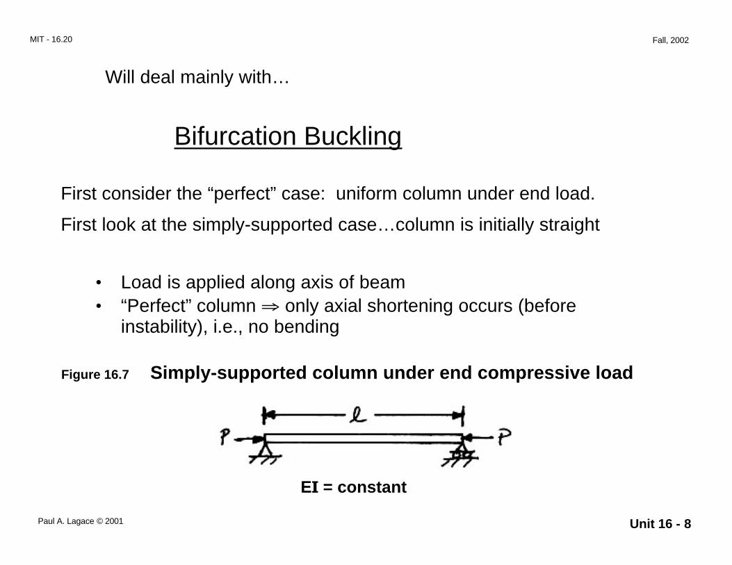
First consider the “perfect” case: uniform column under end load.

First look at the simply-supported case…column is initially straight

• Load is applied along axis of beam • “Perfect” column ⇒ only axial shortening occurs (before

instability), i.e., no bending

Figure 16.7 Simply-supported column under end compressive load

EI = constant


MIT - 16.20 Fall, 2002

Recall the governing equation: 4 2

EId w

+ Pd w

= 0 dx 4 dx2

--> Notice that P does not enter into the equation on the right hand side (making the differential equation homogenous), but enters as a coefficient of a linear differential term

This is an eigenvalue problem. Let: λ xw = e

this gives:

λ4 + P

λ2 = 0 EI

⇒ λ = ± P

EI i 0, 0

repeated roots ⇒ need to look for more solutions

End up with the following general homogenous solution:

w = Asin P

EI x + B cos

P

EI x + C + D x


MIT - 16.20 Fall, 2002

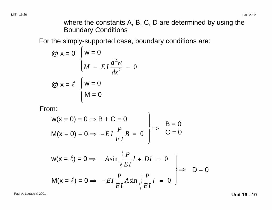
where the constants A, B, C, D are determined by using the Boundary Conditions

For the simply-supported case, boundary conditions are:

@ x = 0 w = 0 2

M = E Id w

= 0 dx2

@ x = l w = 0

M = 0

From:

w(x = 0) = 0 ⇒ B + C = 0 B = 0

⇒ M(x = 0) = 0 ⇒ − E I

PB = 0 C = 0

E I

w(x = l) = 0 ⇒ Asin P

EI l + Dl = 0

⇒ D = 0

M(x = l) = 0 ⇒ − EI P

Asin P

EI l = 0

EI Paul A. Lagace © 2001 Unit 16 - 10

MIT - 16.20 Fall, 2002

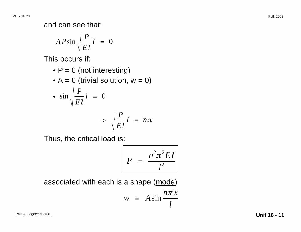
and can see that:

A P sin P

EI l = 0

This occurs if:

• P = 0 (not interesting) • A = 0 (trivial solution, w = 0)

• sin P

EI l = 0

⇒ P

EI l = nπ

Thus, the critical load is:

2 2n π EIP =

l2

associated with each is a shape (mode) n xπ

w = Asin l


MIT - 16.20 Fall, 2002

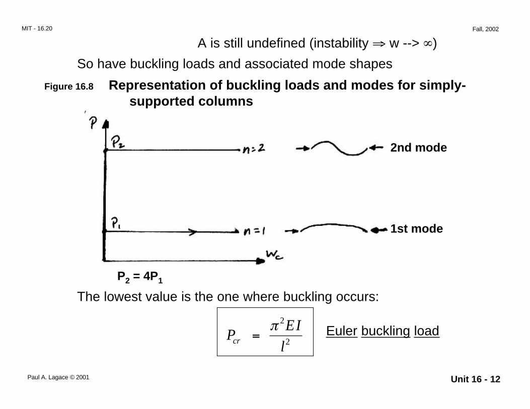
A is still undefined (instability ⇒ w --> ∞)

So have buckling loads and associated mode shapes

Figure 16.8 Representation of buckling loads and modes for simply-supported columns

2nd mode

1st mode

P2 = 4P1

The lowest value is the one where buckling occurs:

P = π 2 EI Euler buckling load

cr l2


MIT - 16.20 Fall, 2002

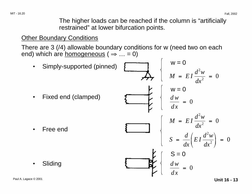
The higher loads can be reached if the column is “artificially restrained” at lower bifurcation points.

Other Boundary Conditions

There are 3 (/4) allowable boundary conditions for w (need two on each end) which are homogeneous ( ⇒ … = 0)

w = 0 • Simply-supported (pinned)

2

M = E Id w

= 0 dx2

w = 0 • Fixed end (clamped) d w

= 0 d x

2

M = E Id w

= 0 dx2

• Free end 2

S = d E I

d w 2 = 0

dx dx

S = 0

• Sliding d w = 0

d x Paul A. Lagace © 2001 Unit 16 - 13

MIT - 16.20 Fall, 2002

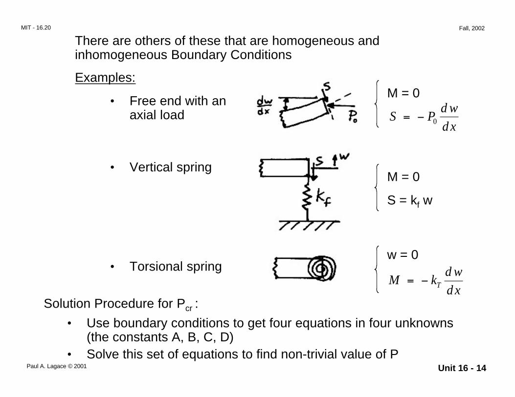
There are others of these that are homogeneous and inhomogeneous Boundary Conditions

Examples:

• Free end with an axial load

• Vertical spring

• Torsional spring

Solution Procedure for Pcr :

M = 0

S = − P d w

0 d x

M = 0

S = kf w

w = 0 d w

M = − kT d x

• Use boundary conditions to get four equations in four unknowns (the constants A, B, C, D)

• Solve this set of equations to find non-trivial value of P Paul A. Lagace © 2001 Unit 16 - 14

MIT - 16.20 Fall, 2002

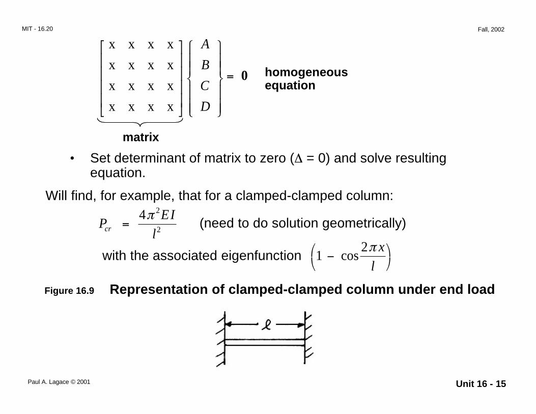
x x x x A x x x x B = 0 homogeneous

x x x x C equation x x x x D

matrix

• Set determinant of matrix to zero (∆ = 0) and solve resulting equation.

Will find, for example, that for a clamped-clamped column: 4π 2 EI

Pcr = l2

(need to do solution geometrically)

with the associated eigenfunction 1 − cos2π x

l

Figure 16.9 Representation of clamped-clamped column under end load


MIT - 16.20 Fall, 2002

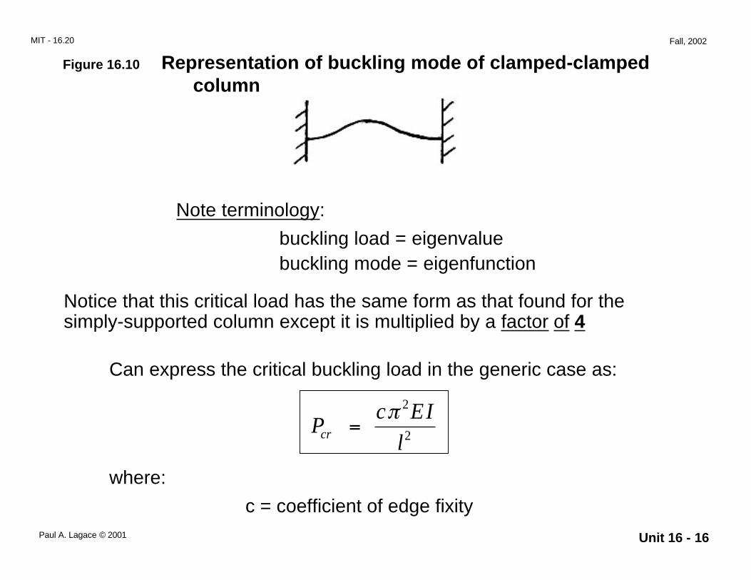
Figure 16.10 Representation of buckling mode of clamped-clamped column

Note terminology:

buckling load = eigenvalue buckling mode = eigenfunction

Notice that this critical load has the same form as that found for the simply-supported column except it is multiplied by a factor of 4

Can express the critical buckling load in the generic case as:

c EIπ 2

P = cr l2

where:

c = coefficient of edge fixity Paul A. Lagace © 2001 Unit 16 - 16

MIT - 16.20 Fall, 2002

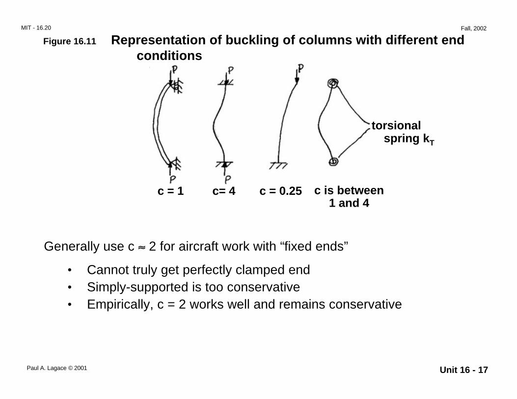
Figure 16.11 Representation of buckling of columns with different end conditions

spring kT

torsional

c = 1 c= 4 c = 0.25 c is between 1 and 4

Generally use c ≈ 2 for aircraft work with “fixed ends”

• Cannot truly get perfectly clamped end • Simply-supported is too conservative • Empirically, c = 2 works well and remains conservative


MIT - 16.20 Fall, 2002

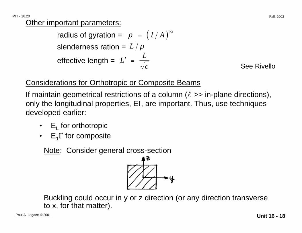
Other important parameters:

radius of gyration = ρ = ( I A 1 2)

slenderness ration = L ρ L

effective length = L′ = c See Rivello

Considerations for Orthotropic or Composite Beams

If maintain geometrical restrictions of a column (l >> in-plane directions), only the longitudinal properties, EI, are important. Thus, use techniques developed earlier:

• EL for orthotropic • E1I* for composite

Note: Consider general cross-section

Buckling could occur in y or z direction (or any direction transverse to x, for that matter).


MIT - 16.20 Fall, 2002

--> must evaluate I* for each direction and see which is less…buckling occurs for the case where I* is smaller

--> anywhere in y-z plane --> use Mohr’s circle

Note: May need to be corrected for shearing effects

See Timoshenko and Gere, Theory of Elastic Stability, pp. 132-135

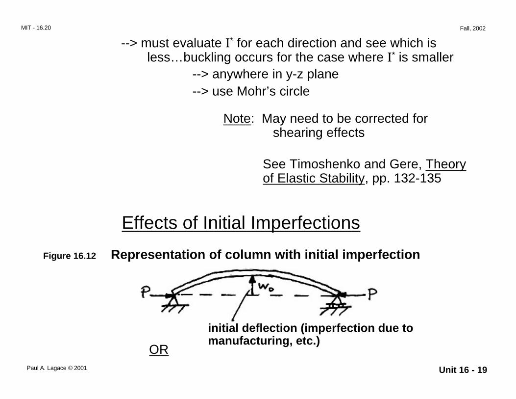
Effects of Initial Imperfections

Figure 16.12 Representation of column with initial imperfection

initial deflection (imperfection due to

OR manufacturing, etc.)


MIT - 16.20 Fall, 2002

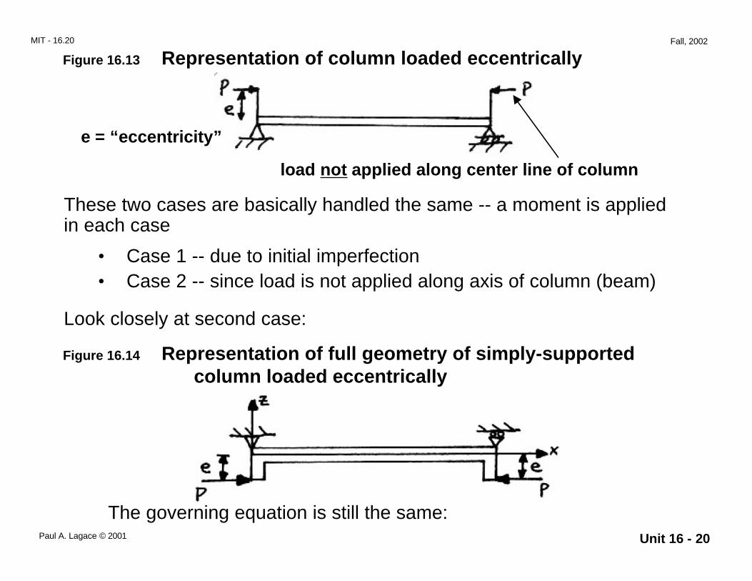
Figure 16.13 Representation of column loaded eccentrically

e = “eccentricity”

load not applied along center line of column

These two cases are basically handled the same -- a moment is applied in each case

• Case 1 -- due to initial imperfection • Case 2 -- since load is not applied along axis of column (beam)

Look closely at second case:

Figure 16.14 Representation of full geometry of simply-supported column loaded eccentrically

The governing equation is still the same:Paul A. Lagace © 2001 Unit 16 - 20

MIT - 16.20 Fall, 2002 4 2

EId w

+ Pd w

= 0 dx 4 dx2

and thus the basic solution is the same:

w = Asin P

EI x + B cos

P

EI x + C + D x

What changes are the Boundary Conditions

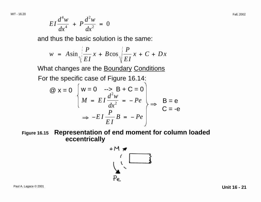
For the specific case of Figure 16.14:

@ x = 0 w = 0 --> B + C = 0 2

M = E Id w

= − Pe ⇒ B = e

dx2

C = -eP ⇒ −E I B = − Pe

E I

Figure 16.15 Representation of end moment for column loaded eccentrically


MIT - 16.20 Fall, 2002

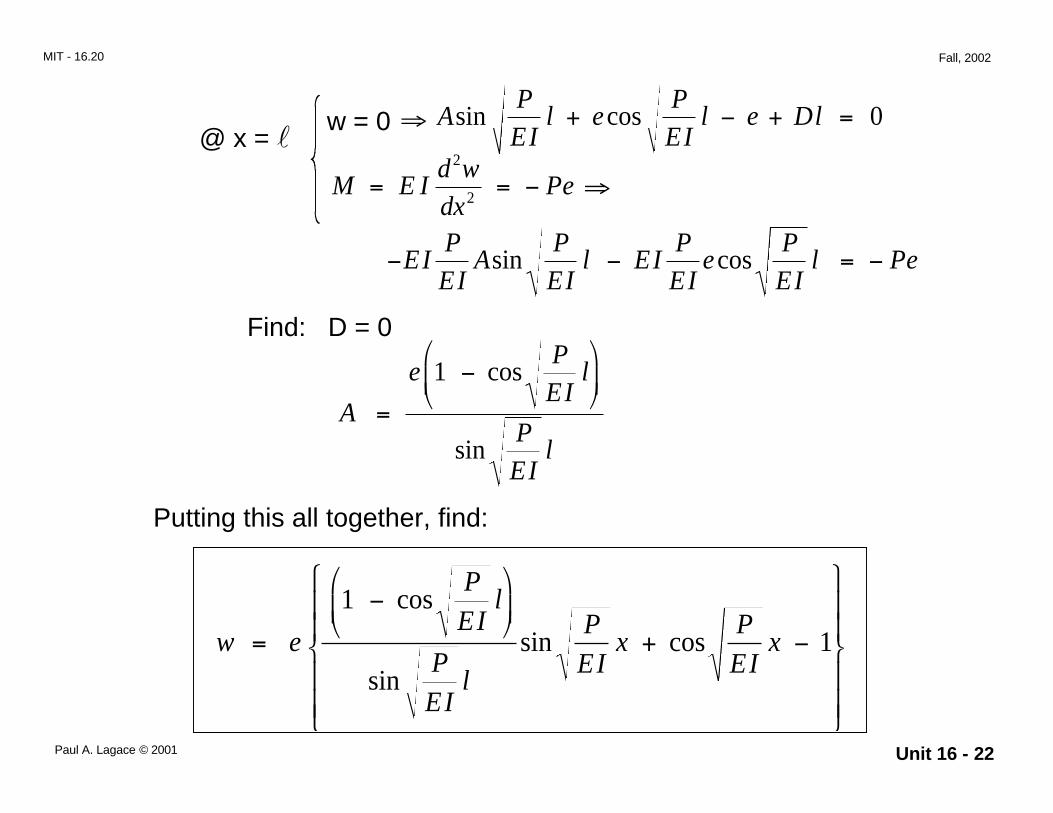
w = 0 ⇒ Asin P

EI l + e cos

P

EI l − e + Dl = 0

@ x = l 2

M = E Id w

= − Pe ⇒dx2

−EI P

Asin P

EI l − EI

Pe cos

P

EI l = − Pe

EI EI

Find: D = 0 P

EI

e 1 − cos l

A = sin

P

EI l

Putting this all together, find:

w

P

EI l

P

EI l

P

EI x

P

EI x=

−

+ −

1

1

cos

sin sin cos e


MIT - 16.20 Fall, 2002

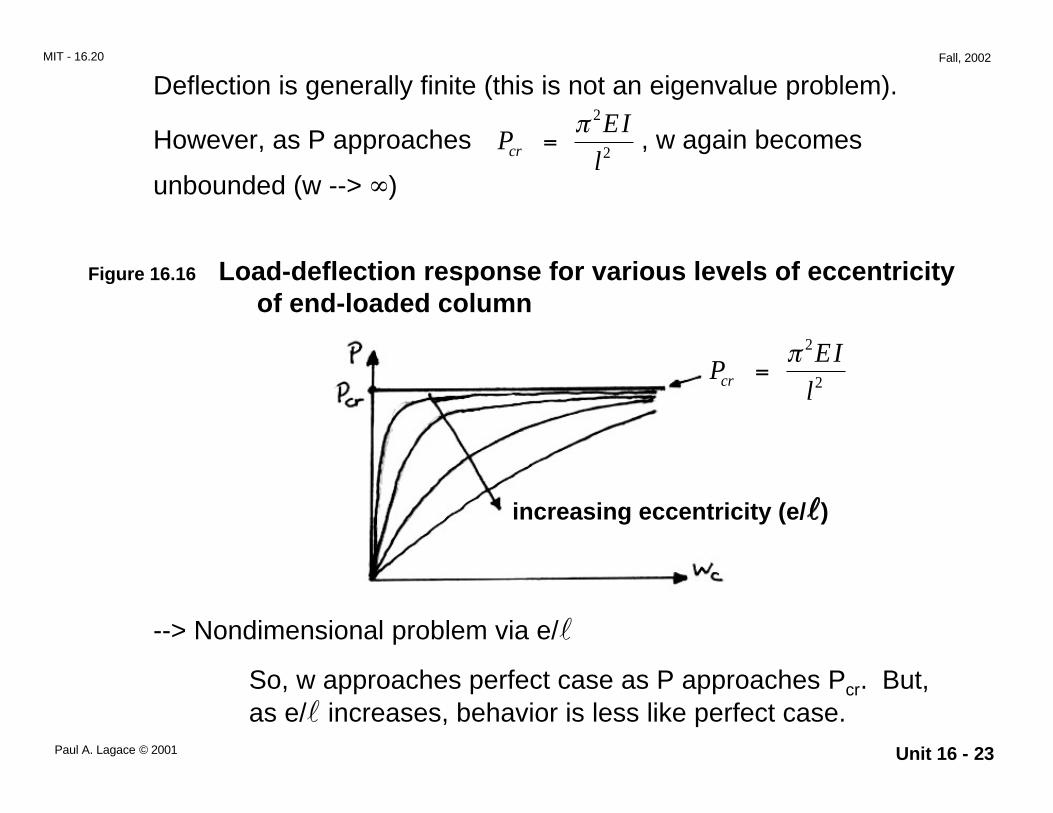
Deflection is generally finite (this is not an eigenvalue problem). π 2 EI

However, as P approaches Pcr = l2

, w again becomes

unbounded (w --> ∞)

Figure 16.16 Load-deflection response for various levels of eccentricity of end-loaded column

π 2 EI =

l2Pcr

increasing eccentricity (e/llll)

--> Nondimensional problem via e/l

So, w approaches perfect case as P approaches Pcr. But, as e/l increases, behavior is less like perfect case.


MIT - 16.20 Fall, 2002

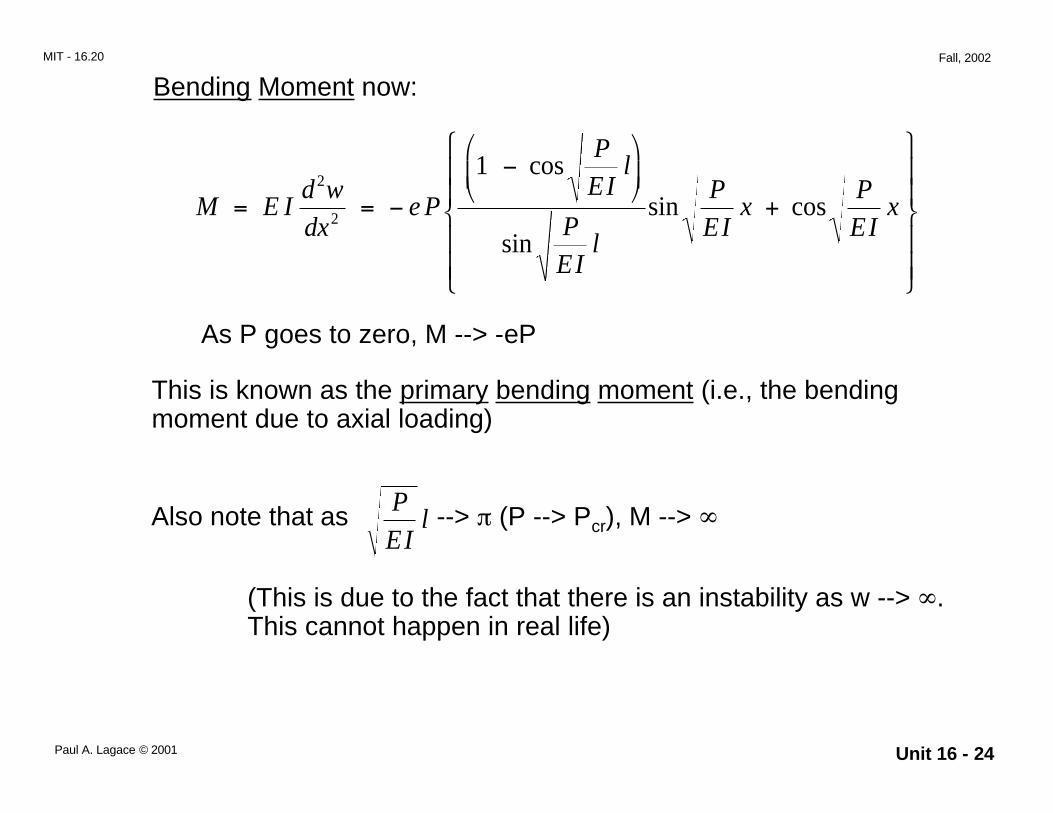
Bending Moment now:

P

EI

1 − cos l

P

EI

P

EI

2 M = E I

d w = − e P

P

EI

sin x + cos x dx2

sin l

As P goes to zero, M --> -eP

This is known as the primary bending moment (i.e., the bending moment due to axial loading)

Also note that as P

EI l --> π (P --> Pcr), M --> ∞

(This is due to the fact that there is an instability as w --> ∞. This cannot happen in real life)


MIT - 16.20 Fall, 2002

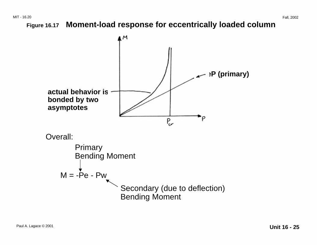
Figure 16.17 Moment-load response for eccentrically loaded column

eP (primary)

actual behavior is bonded by two asymptotes

Overall: Primary Bending Moment

M = -Pe - Pw

Secondary (due to deflection) Bending Moment


MIT - 16.20 Fall, 2002

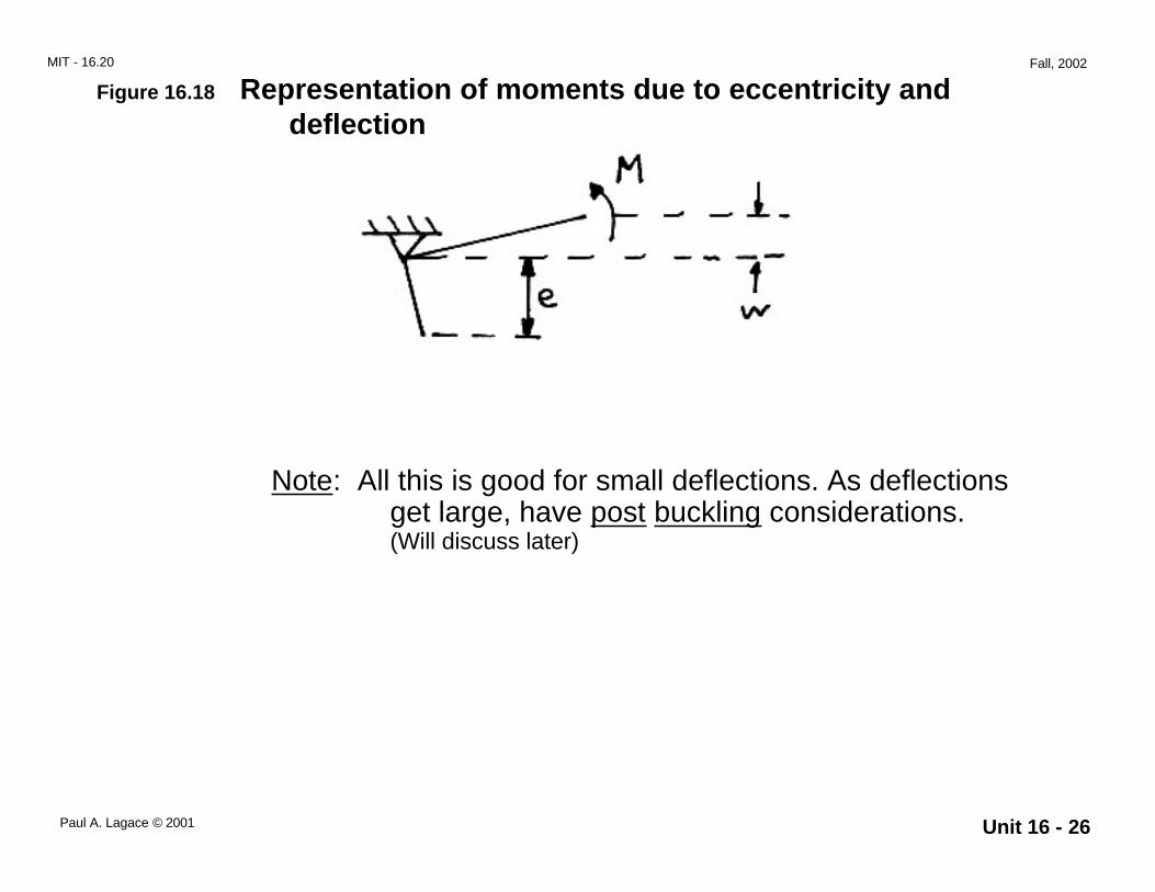
Figure 16.18 Representation of moments due to eccentricity and deflection

Note: All this is good for small deflections. As deflections get large, have post buckling considerations. (Will discuss later)


professor of aeronautics & astronautics bifurcation buckling · pdf file ·...

Documents