producer theory - cms.phbs.pku.edu.cn

Producer Theory

Marshall Urias

Marshall Urias Producer Theory 1 / 79

Theory of the firm

The theory of the firm explains how businesses make profit-maximizingdecisions in the face of constraints related to technology and themarketplace.

We will tackle the theory of the firm in different parts:

1 Production technology

2 Cost constraints

3 Input choices


Part 1: Technology


Technology

Technology describes the feasible means of converting raw inputs, calledfactors of production, into output.


Factors of production

Factors of production are often classified into broad categories such as

Labor

Capital

Land

Materials

When economists talk about capital, we mean inputs to production thatare themselves produced goods (e.g. buildings, computers, machinery).

Sometimes the word “capital” is uesed to describe the start-up moneyrequired for a business, but here we use the word “capital” to refer tophysical capital, not financial capital.


Production set

The set of all combinations of inputs and outputs that are technologicallyfeasible is called a production possibilities set.

It is most useful to think of inputs and outputs as being measured in termsof flows: a certain amount of inputs per time period are used to produce acertain amount of outputs per unit of time period.

Formally, we can show a production plan by a vector y ∈ Rn where yj < 0represents the jth good is an input, and yj > 0 represents the jth good isan output. The set of all patterns of inputs and outputs that aretechnologically feasible, Y ⊂ Rn, is called the production possibilitiesset.


Production set

Note that you can describe the elements of a production plan witharbitrary specificity and distinguish between plans that are “immediatelyfeasible” versus “eventually feasible.”

We may choose to distinguish between skilled and unskilled labor, or evenprofessors and administrative workers, or even assistant professors andassociate professors and 114 workers and HR workers, and so on...

We may choose to distinguish the short-run from the long-run based onwhich production plans are feasible today versus sometime in the future.


Input set

Example: Suppose we have a firm that produces only one output y using avector of inputs x . We can then define a special case of restrictedproduction possibilities set called the input requirement set

V (y) = {x ∈ Rn+ : (y ,−x) is inY }

The input requirement set is the set of all input bundles that produce atleast y units of output.


Isoquants

In the previous example, we could also define an isoquant

Q(y) = {x ∈ Rn+ : x is inV (y) and x is not in V (y ′) for y ′ > y}

The isoquant gives all input bundles that produce exactly y units ofoutput.


Production function

When a firm has only one output, we can easily describe what istechnologically feasible using a production function

f (x) = {y ∈ R : y is the maximum output associated with − x}

The production function describes what is technologically feasible whenthe firm operates efficiently—when the firm uses each combination ofinputs as effectively as possible.


Production set


Cobb-Douglas technology

One of the most widely studied production technologies is theCobb-Douglas technology. Let α, β ∈ (0, 1) and A > 0 and supposeonly two inputs, then the technology is defined by

Y = {(y , x1, x2) : y ≤ Axα1 xβ2 }

V (y) = {(x1, x2) : y ≤ Axα1 xβ2 }

Q(y) = {(x1, x2) : y = Axα1 xβ2 }

f (x1, x2) = Axα1 xβ2

The parameter A measures, roughly speaking, the scale of production whilethe parameters α, β dictate how output responds to changes in inputs.


Cobb-Douglas technology


Fixed proportion (Leontif) technology

Another popular technology is described by the following

Y = {(y , x1, x2) : y ≤ min(ax1, bx2)}V (y) = {(x1, x2) : y ≤ min(ax1, bx2)}Q(y) = {(x1, x2) : y = min(ax1, bx2)}

f (x1, x2) = min(ax1, bx2)

where a, b > 0.


Fixed proportion (Leontif) technology


Perfect substitutes technology

Another popular technology is described by the following

Y = {(y , x1, x2) : y ≤ x1 + x2}V (y) = {(x1, x2) : y ≤ x1 + x2)}Q(y) = {(x1, x2) : y = x1 + x2}

f (x1, x2) = x1 + x2


Perfect substitutes technology


Properties of technology

As was done for preferences, it is useful to assume some reasonableproperties about technology:

Monotonic: if you increase the amount of at least one of the inputs,it should be possible to produce at least as much output as you wereproducing before

Convex: if you have two ways to produce y units of output, say(x1, x2) or (z1, z2), then their weighted average will produce at leasty units of output.



Why convexity?

Suppose there are two different techniques a firm can use to produce 1unit of output

Technique A: one unit of factor 1 and two units of factor 2

Technique B: two units of actor 1 and one unit of factor 2

and suppose we want to produce 100 units of output.

As a first step, we can argue that we should be able to replicate how weproduce 1 unit of output 100 times. Of course not all production processeswill allow for this kind of replication, but it seems plausible in manycircumstances. So we conclude that (100,200) and (200,100) are inV (100).



Of course, we could also replicate 50 processes of technique A and 50processes of technique B using (150, 150), or 25 processes of technique Aand 75 processes of technique B using.25(100, 200) + .75(200, 100) = (175, 125) or ...

t(100, 200) + (1− t)(200, 100) = (100t + 200(1− t), 200t + (1− t)100)

all of which belong to V (100).


Convexity


The average product

One way to measure how useful each input is in the production process isto use the average product—output per unit of a particular unit. Theaverage product of factor i is

APi =y

xi=

f (x)

xi


The marginal product

Given some technology, we want to quantify how much extra output canbe generated from increasing inputs.

The question economists ask is: How much more output will we get peradditional unit of factor i, holding factor j constant?

The answer is called the marginal product of factor i:

MPi ≡∂y

∂xi=∂f (x)

∂xi


The marginal product

We often assume diminishing marginal product—as the use of an inputincreases with other input fixed, the marginal additions to output willeventually decrease—because it is a common feature of most kinds ofproduction processes.

Imagine 1 person working in office 114 can service 50 students per week.If we add another person to the office, we may be able to service 100students per week, in which case we say the marginal product of an extraworker is 50 students. You can imagine what happens when we try to hirethe 50th person!


Relationship between average and marginal

We have a very useful relationship between the average product andmarginal product:

∂APi

∂xi=∂f (x)

∂xi

1

xi− f (x)

x2i=

MPi − APi

xi

Therefore we have that

if MPi > APi then average product is increasing

if MPi = APi then average product is constant

if MPi < APi then average product is decreasing


The technical rate of substitution

Given some technology, we want to quantify how the firm can vary its mixof inputs to produce the same amount of output.

The question economists ask is: How much extra factor j do we need if weare going to give up a little bit of factor i in order to produce the sameamount of output?

The answer is called the technical rate of substitution

TRS(xi , xj) =∂xj∂xj

= −MPi

MPj

Notice that this is the slope of the isoquant!


The technical rate of substitution

We often assume diminishing technical rate of substitution because itis a common feature of most kinds of production processes.

The isoquants will have the same sort of convex shape as well-behavedindifference curves.

Example: Food grown on large farms in the United States, where labor isrelatively expensive, operate in the range of production where the rate oftechnical substitution is high (high capital-to-labor ratio), whereas indeveloping countries, where labor is cheap, operate with a lower rate oftechnical substitution (lower capital-to-labor ratio).


Returns to scale

Instead of increasing the amount of one output while holding the otherinput fixed, we can measure what happens when we increase the amountof all inputs to the production function. In other words, let’s scale theamount of inputs up by a constant factor: for example, use twice as muchof all factors.

Constant returns to scale: tf (x) = f (tx)

Increasing returns to scale: tf (x) > f (tx)

Decreasing returns to scale: tf (x) < f (tx)


Returns to scale

Constant returns to scale is the most “natural” case because of thereplication argument.

Increasing returns to scale occurs for some production technologies such asoil pipeplines (if we double the diameter of the pipe, we use twice as muchmaterial, but the cross section of the section of the pipe goes up by afactor of 4!)

Decreasing returns to scale seems “unnatural” because of the replicationargument, but makes sense in the short-run if some inputs are fixed.

It may be the case that technology can exhibit different kinds of returns toscale at different levels of production (if you try to keep increasing thediameter of the pipeline eventually it will collapse under it’s ownweight...maybe the same for 114 )


Part 2: Profit Maximization


Profit

Economic profit is the difference between revenues and costs.

It is important to remember that all costs must be included in thecalculation of economic profit:

If I open a noodle shop in Pingshan and work there, my salary as anemployee should be counted as a cost of production

If my students loan me money to open the noodle shop, the interestpayment must be counted as a cost of production

If I need to bribe a health regulator to let me keep my shop open, thebribe money should be counted as a cost


Accounting versus economic profit

Accounting profit = revenues minus explicit costs. Costs associated withpaying wages to workers, buying raw materials etc.

Economic profit = revenues minuse implicit and explicit costs. Implicitcosts include the opportunity cost of production.


Accounting versus economic profit

I’m considering leaving my job at PHBS to open a noodle shop inPingshan

I earn 40,000 RMB per month at PHBS

I forecast 10,000 RMB per month revenue from the noodle business

I forecast rent and other expenses at 7,000 RMB per month

Accounting profit = 10,000 - 7,000 = 3,000 RMB per month

Economic profit = 10,000 - 7,000 - 40,000 = -37,000 RMB per month


Profit

At an abstract level we can imagine that a firm can engage in a largevariety of actions, all of which incur costs. We can write the revenue as afunction of some n actions, R(a1, ..., an), and the costs as a function ofthese same n activities C (a1, ..., an).

The most basic assumption of the economic analysis of the firm is that itacts to as to maximize profits

maxa1,...,an

R(a1, ..., an)− C (a1, ..., an)


Fundamental concept of profit maximization

Taking first order conditions reveals the most fundamental conditioncharacterizing profit maximization:

∂R(a∗)

∂ai=∂C (a∗)

∂ai

The level of output should be chosen so that the production of one moreunit of output should produce a marginal revenue equal to its marginalcost.


Fundamental concept of profit maximization

Example: Suppose a company is deciding how many employees to hire thisyear. Our fundamental condition for profit maximization says that thecompany should hire an amount of labor such that the marginal revenuefrom employing one more person is equal to the marginal cost of hiringthat person.


Profit maximization

In order to apply this concept in a more concrete way, we need to break uprevenues and costs into different parts:

Revenue consists of how much output the firm sells and the price ofthat output

Costs consists of how much input the firm buys and the prices ofthose inputs

There are market constraints that concern the effect of actions of otherentities on the firm. For now, we assume the simplest kind of marketbehavior called price-taking behavior. That is, each firmm will beassumed to take prices as given, exogenous variables. Such a price-takingfirm is called a competitive firm.


Profit maximization

The most general way of describing the firm’s problem is

π(p) = maxpy s.t. y ∈ Y

but for us it will be mostly sufficient to focus on the case of a singleoutput firm

π(p,w) = maxx

pf (x)−wx

or if you like the two input case we could write

π(p,w1,w2) = maxx1,x2

pf (x1, x2)− w1x1 − w2x2


Profit maximization

The firm chooses how much of each input x = (x1, ..., xn) to use, takingprices p and w = (w1, ...,wn) as given, to maximize profits. We can nowexpress the profit maximization condition concretely

p∂f (x)

∂xi= wi

The value of the marginal product of each factor must be equal to its price.


Fixed versus variable factors

In a given period of time, it may be very difficult to adjust some of theinputs. We call a factor of production that is used in a fixed amount as afixed factor, while a factor that can be used in different amounts is calleda variable factor.

Economists often distinguish the long-run from the short-run based onwhether or not some factors are fixed. If a firm is unable to adjust some ofit’s factors, then we say that this is the short-run for the firm. In thelong-run, all factors are variable.



We may then distinguish a firm’s short-run profit maximization problem as

maxx1

pf (x1, x̄2)− w1x1 − w2x̄2

which of course yields the same rule as before

pMP1(x∗1 , x̄2) = w1


Factor demands

The functions that give the optimal choices of inputs for given prices areknown as factor demands, denoted xi (p,w), which are defined implicitlyby our profit maximizing condition

∂f (x)

∂xi=

wi

p

We want to know how these factor demands behave...


Factor demands

For simplicity, let’s look at a firm with one output and one input

maxx

pf (x)− wx

We know the factor demand function x(p,w) must satisfy

pf ′(x(p,w))− w = 0

pf ′′(x(p,w)) ≤ 0

We can differentiate the first-order condition to get

dx(p,w)

dw=

1

pf ′′(x(p,w))

So factor demands slope downward!


Part 3: Costs of Production


Cost minimization problem

Here we study how firms make decisions to produce a given amount ofoutput at minimum cost.

minx

wx s.t. f (x) = y



The two most important costs facing a firm are labor and capital.

The price of labor is simply the wage rate w

The price of capital is called the rental rate r . Capital that ispurchased can be treated as though it were rented at a rental rateequal to the interest rate plus depreciation rate.

Often we can discuss the costs of the firm only in terms of these twovariables

TC = wL + rK

but more generally we can specify an arbitrary number of inputs

TC = wx



Writing the Lagrangian for the cost minimization problem

L = wx − λ[f (x)− y ]

allows us to take first order conditions characterizing an interior solution x∗

wi − λ∂f (x∗)

∂xi= 0 for i = 1, ..., n

f (x∗) = y



We can interpret these first-order conditions by dividing the ith conditionby the jth to get

wi

wj=

∂f (x∗)∂xi

∂f (x∗)∂xj

which says that a firm will employ each factor such that it’s marginal rateof technical substitution is equal to the economic rate of substitution. Ifthis were not so, then there would exist some adjustment that could lowercosts while still producing the same output, for example

wi

wj=

2

16= 1

1=

∂f (x∗)∂xi

∂f (x∗)∂xj

could save two dollars by hiring one unit less of factor i and spend onlyone extra dollar by hiring more of factor j .



Example: Consider a firm just employing capital K and labor L.

Our cost minimizing condition is that

MRTS =MPL

MPK=

w

r

Given the wage rate and rental rate, the firm optimally chooses acombination of labor and capital such that the rate of technicalsubstitution is exactly equal to the wage-to-rental-rate ratio.


Long-run total cost curve

The conditional factor demands are the functions that give the optimalchoices of inputs for given prices and output x(w , y).

The total cost function shows the minimal cost of producing y units ofoutput

c(w , y) ≡ wx(w , y)

which is just the value of the conditional factor demands.



We can illustrate the total cost function in the following way

Choose an output level y represented by an isoquant

Find the point of tangency of your chosen isoquant with an isocostline

From the isocost line, determine the cost of producing y

Graph the output-cost combination


Short-run total cost curve

The short-run cost function is simply the minimum cost of producing youtput, only adjusting variable factors of production

cs(wv ,wf , y) ≡ wvxv (wv ,wf , y) + wf xf (wv ,wf , y)


Fixed versus variable costs

It is useful to distinguish between different types of costs that firms face:

Variable costs: costs that vary with the level of output

Fixed costs: costs that are independent of the level of output

Quasi-fixed costs: costs that that are independent of the level ofoutput, but only need to be paid if the firm produces a positiveamount of output

Sunk costs: a cost that has already been incurred before the level ofproduction is decided


Fixed versus variable costs

We can always express total costs of the firm as the sum of the variablecosts and fixed costs

c(y) = cv (y) + F

(where it is understood that costs depend on factor prices, but we takethese as exogenous and fixed for now)


Average cost

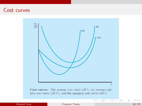
The average cost function measures the cost per unit of output.

AC (y) =c(y)

y=

cv (y)

y+

F

y= AVC (y) + AFC (y)


Average cost


Average cost

Notice that...

...if technology exhibits increasing returns to scale, then the costs willincrease less than linearly with respect to output, so the average costswill be declining in output

...if technology exhibits decreasing returns to scale, then averagecosts will rise as output increases

...if technology exhibits constant returns to scale, then average costswill unchanged as output increases


Average cost

When evaluating whether producing an extra unit is worthwhile, the firmcares about marginal cost

MC (y) ≡ c ′(y)


Cost curves


Long-run and short-run cost curves

We define the short-run as being the period of time in which the firm isunable to adjust some factors, so that there exist fixed costs.

In the long-run, the firm can choose the level of “fixed” factors—they areno longer fixed!

Although there may be quasi-fixed costs in the long-run—costs that haveto be paid to produce any positive level of output—there are no fixedcosts, since it is always possible to shut down.



Suppose I’m deciding on expanding my Pingshan noodle shop. Let’simagine the fixed factor as being the total square meters of real estate Iown in shop-space (call it k). In the short-run, I can easily vary laborhours, ingredient purchases, operating time etc, but I can’t quicklypurchase new real estate. Denote my noodle shop’s short-run costfunction by

cs(y , k̄)

For any given target level of output, there is some optimal size of realestate to produce that level of output, call it k(y). Then the long-run costfunction for my noodle shops is

c(y) = cs(y , k(y))



Notice that she short-run cost of running my noodle shops to produce y ,must be at least a large as the long-run cost to produce y , because in thelong-run I’m able to adjust the size of my real estate.

And at my desired level of real-estate, my short-run cost will be exactlyequal to my long-run cost.


Part 4: Supply


Market constraints

So far we have discussed the technological constraints facing a firm, andhow technology leads to cost constraints.

Now we consider market constraints—the competitive environment thatlimits the firms ability to sell according to how much people are willing tobuy.

In fact, we have already described an important element of a marketconstraint: the demand curve!


Market constraints

If there were only one firm in the market, the demand curve facing thefirm is easy to describe: it is just the market demand curve describedearlier on consumer behavior.

But if there are other firms in the market, the market constraints facingthe firm will be different. In this case, the firm has to guess how the otherfirms in the market will behave when it chooses its price and output.


Market constraints

For now, let’s analyze the simplest market environment called purecompetition.

Large number of buyers and sellers.

Homogeneous output. All firms sell identical product

Perfect information. Buyers and sellers have all information about themarket

No transaction costs. Neither buyers nor sellers incur costs or fees toparticipate in the market

No externalities. Each firm bears the full cost of its productionprocess.


Market constraints

The key implication of the pure competition market environment is thateach individual firm is a price taker: the price is taken as given by anyindividual firm.

No firm can charge a price above the market price without losing all of itscustomers, so the firm views the price at which it can sell as beyond itscontrol. Similarly, consumers cannot find a firm willing to sell blwo marketprice, so conusmer also view the market price as beyond their contorl.


Firm’s demand curve

A price-takers demand curve is simple:

If it sells at the market price, it can sell whatever amount it wants

If it sells below the market price, it will get the entire market demandat that price

Don’t forget we are describing the demand curve facing a particular firm.This is not the same as the market demand curve which measures therelationship between the market price and the total output sold.


Firm’s demand curve


Price-taking firm’s supply decision

Because we are analyzing a market environment where firms are pricetakers, profit maximization problem facing a firm is

maxy

py − c(y)

which obtains an optimal amount of output y∗ given by the rule

p = MC (y)

Notice that this is a simple application of the rule we learned before: profitmaximization occurs where marginal revenue equals marginal cost. Here,the marginal revenue of a firm is simply the price it can sell it’s output,which is independent of output due to price-taking behavior.



Whatever is the market price, a competitive firm will choose a level ofoutput y such that price equals marginal cost.

The marginal cost curve of a competitive firm is precisely its supply curve.


producer theory - cms.phbs.pku.edu.cn

Documents