Probability Distribution

Prof. (Dr.) Rajib Kumar BhattacharjyaIndian Institute of Technology Guwahati

Guwahati, Assam

Email: rkbc@iitg.ernet.in Web: www.iitg.ernet.in/rkbc

Visiting Faculty NIT Meghalaya

Probabilistic Approach:

A random variable X is a variable described by a probability distribution.

The distribution specifies the chance that an observation x of the variable will fall in a specific range of X.

A set of observations n1, n2, n3,…………., nn of the random variable is called a sample.

It is assumed that samples are drawn from a hypothetical infinite population possessing constant statistical

properties.

Properties of sample may vary from one sample to others.

The probability P (A) of an event is the chance that it will occur when an observation of the random variable is made.

𝑃(𝐴) = lim𝑛→∞

𝑛𝐴

𝑛

nA --- number in range of event A.

n----- Total observations

1. Total Probability

𝑃 𝐴1 + 𝑃 𝐴2 + 𝑃 𝐴3 +. . ……………+ 𝑃(𝐴𝑛) = 𝑃(Ω) = 1

1. Complementarity

𝑃 𝐴 = 1 − 𝑃(𝐴)

1. Conditional Probability

𝑃𝐵

𝐴=

𝑃(𝐴∩𝐵)

𝑃(𝐴)

B will occur provided A has already occurred.

Joint Probability

𝑃 𝐴 ∩ 𝐵 = 𝑃(𝐴)𝑃(𝐵)

Example:

The probability that annual precipitation will be less than 120 mm is 0.333. What is the probability that there will be

two successive year of precipitation less than 120 mm.

P(R<35) = 0.333

P(C) = 0.3332 =0.111

Year

Precipi-tation

2

5

9

15

10

5

Frequency Histogram

Relative Frequency:

𝑓𝑠 𝑥𝑖 =𝑛𝑖

𝑛

Which is equivalent to 𝑃 𝑥𝑖 − ∆𝑥 ≤ 𝑋 ≤ 𝑥𝑖 , the probability that the random variable X will lie in the interval [𝑥𝑖 −

∆𝑥,𝑥𝑖]

Cumulative Frequency Function:

𝐹𝑠 𝑥𝑖 =

𝑗=1

𝑖

𝑓𝑠 𝑥𝑗

This is estimated as 𝑃 𝑋 ≤ 𝑥𝑖 , the cumulative probability of xi.

This is estimated for sample data, corresponding function for population will be

Probability density Function:

𝑓 𝑥 = lim𝑛→∞∆𝑥→0

𝑓𝑠(𝑥)

∆𝑥

Probability Distribution Function:

𝐹 𝑥 = lim𝑛→∞∆𝑥→0

𝐹𝑠 𝑥

Whose derivative is the probability density function

𝑓 𝛾 =𝑑𝐹 𝛾

𝑑𝑥

The cumulative probability as 𝑃 𝑋 ≤ 𝑥 , can be expressed as

𝑃 𝑋 ≤ 𝑥 = 𝐹 𝑥 =

−∞

𝑥

𝑓 𝑢 𝑑𝑢

𝑃 𝑥𝑖 = 𝑃 𝑥𝑖 − ∆𝑥 ≤ 𝑋 ≤ 𝑥𝑖

=

𝑥𝑖−∆𝑥

𝑥𝑖

𝑓 𝑥 𝑑𝑥

=

−∞

𝑥𝑖

𝑓 𝑥 𝑑𝑥 −

−∞

𝑥𝑖−∆𝑥

𝑓 𝑥 𝑑𝑥

=𝐹 𝑥𝑖 − 𝐹 𝑥𝑖 − ∆𝑥

=𝐹 𝑥𝑖 − 𝐹 𝑥𝑖−1

Sample

Pxi

fsxi

∆xx xi

Population

Fsxi

x

Fsxi

dF(x)

dx

Probability density function

𝑓(𝑥)

𝑥

𝐹(𝑥)

𝑥

𝑓 𝑥 =1

2𝜋𝑒𝑥𝑝 −

𝑥 − 𝜇 2

2𝜎2

𝑓 𝑧 =1

2𝜋𝑒𝑥𝑝 −

𝑧2

2 𝑧 =𝑥 − 𝜇

𝜎

𝐹 𝑧 =

−∞

𝑧1

2𝜋𝑒−𝑢2/2𝑑𝑢

−∞ ≤ 𝑧 ≤ ∞

𝐹 𝑧 =

−∞

𝑧1

2𝜋𝑒−𝑢2/2𝑑𝑢

Cumulative probability of standard normal distribution

𝐵 =1

21 + 0.196854 𝑧 + 0.115194 𝑧 2 + 0.000344 𝑧 3 + 0.019527 𝑧 4 −4

𝐹 𝑧 = 𝐵 for 𝑧 < 0

𝐹 𝑧 = 1 − 𝐵 for 𝑧 ≥ 0

Ex. What is the probability that the standard normal random variable 𝑧 will be less than -2? Less than 1? What is 𝑃 −2 < 𝑍 < 1 ?

𝑃 𝑍 < −2 = 𝐹 −2 = 1 − 𝐹 2 = 1 − 0.9772 = 0.228

Solution

𝑃 𝑍 < 1 = 𝐹 1 = 0.8413

𝑃 −2 < 𝑍 < 1 = 𝐹 1 − 𝐹 2 = 0.841 − 0.023 = 0.818

Example 2:

The annual runoff of a stream is modeled by a normal distribution with mean and standard deviation of 5000 and 1000 ha-m

respectively.

i. Find the probability that the annual runoff in any year is more than 6500 ha-m.

ii. Find the probability that it would be between 3800 and 5800 ha-m.

Solution:

Let X is the random variable denoting the annual runoff. Then z is given by

𝑧 =(𝑋−5000)

1000N (0, 1)

(i) P (X≥6500) = P (z ≥(6500−5000)

1000)

= P (z≥1.5)

= 1-P (z≤1.5)

= 1- F (1.5)

F (1.5) = 0.9332

P (X≥6500) =1-0.9332 = 0.0688

P (X≥6500) =0.0688

(ii) P (3800≤X≤5800)

= P [(3800−5000)

1000≤ 𝑧 ≤ P

(5800−5000)

1000]

= P [-1.2≤z≤0.8]

= F (0.8)-F (-1.2)

= F (0.8)-[1-F (1.2)]

=0.7881-(1-0.8849)

=0.673

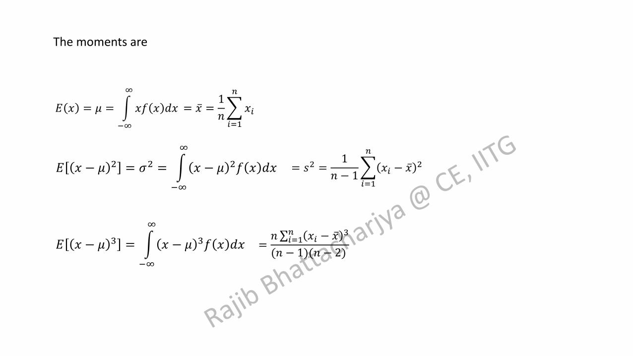
Statistical parameter

Expected value

It is the first moment about the origin of the random variable, a measure of the midpoint or central tendency of the distribution

The sample estimate of the mean is the average

The variability of data is measured by the variance 𝜎2

𝐸 𝑥 − 𝜇 2 = 𝜎2 =

−∞

∞

𝑥 − 𝜇 2𝑓 𝑥 𝑑𝑥

𝐸 𝑥 = 𝜇 =

−∞

∞

𝑥𝑓 𝑥 𝑑𝑥

𝑥 =1

𝑛

𝑖=1

𝑛

𝑥𝑖

The sample estimate of the variance is given by 𝑠2 =1

𝑛 − 1

𝑖=1

𝑛

𝑥𝑖 − 𝑥 2

A symmetry of distribution about the mean is a measured by the skewness. This is the third moment about the mean

𝐸 𝑥 − 𝜇 3 =

−∞

∞

𝑥 − 𝜇 3𝑓 𝑥 𝑑𝑥

The coefficient of skewness 𝛾 is defined as

𝛾 =1

𝜎3𝐸 𝑥 − 𝜇 3

A sample estimate for 𝛾 is given by

𝐶𝑠 =𝑛 𝑖=1

𝑛 𝑥𝑖 − 𝑥 3

(𝑛 − 1)(𝑛 − 2)𝑠3

Fitting a probability distribution

A probability distribution is a function representing the probability of occurrence of a random variable.

By fitting a distribution function, we can extract the probabilistic information of the random variable

Fitting distribution can be achieved by the method of moments and the method of maximum likelihood

Method of moments

Karl Pearson (27 March 1857 – 27 April 1936) was an English mathematician

Developed by Karl Pearson in 1902

He considered that good estimate of the parameters of a probability distribution are those for which moments of the probability density function about the origin are equal to the corresponding moments of the sample data

𝐸 𝑥 − 𝜇 2 = 𝜎2 =

−∞

∞

𝑥 − 𝜇 2𝑓 𝑥 𝑑𝑥

𝐸 𝑥 = 𝜇 =

−∞

∞

𝑥𝑓 𝑥 𝑑𝑥 = 𝑥 =1

𝑛

𝑖=1

𝑛

𝑥𝑖

= 𝑠2 =1

𝑛 − 1

𝑖=1

𝑛

𝑥𝑖 − 𝑥 2

𝐸 𝑥 − 𝜇 3 =

−∞

∞

𝑥 − 𝜇 3𝑓 𝑥 𝑑𝑥 =𝑛 𝑖=1

𝑛 𝑥𝑖 − 𝑥 3

(𝑛 − 1)(𝑛 − 2)

The moments are

Method of moments

Developed by R A Fisher in 1922 Sir Ronald Aylmer Fisher (17 February 1890 –29 July 1962), known as R.A. Fisher, was an Englishstatistician, evolutionarybiologist, mathematician,geneticist, and eugenicist.

He reasoned that the best value of a parameter of a probability distribution should be that value which maximizes the likelihood of joint probability of occurrence of the observed sample

Suppose that the sample space is divided into intervals of length 𝑑𝑥 and that a sample of independent and identically distributed observations 𝑥1, 𝑥2, 𝑥3, … , 𝑥𝑛 is taken

The value of the probability density for 𝑋 = 𝑥𝑖 is 𝑓(𝑥𝑖)

The probability that the random variable will occur in that interval including 𝑥𝑖 is 𝑓 𝑥𝑖 𝑑𝑥

Since the observation is independent, their joint probability of occurrence is

𝑓 𝑥1 𝑑𝑥𝑓 𝑥2 𝑑𝑥𝑓 𝑥3 𝑑𝑥 …𝑓 𝑥𝑛 𝑑𝑥 =

𝑖=1

𝑛

𝑓(𝑥𝑖)𝑑𝑥𝑛

𝑀𝑎𝑥 𝐿 =

𝑖=1

𝑛

𝑓(𝑥𝑖)

Since 𝑑𝑥 is fixed, we can maximize

𝑀𝑎𝑥 𝑙𝑛𝐿 =

𝑖=1

𝑛

𝑙𝑛𝑓(𝑥𝑖)

Example: The exponential distribution can be used to describe various kinds of hydrological data, such as

inter arrival times of rainfall events. Its probability density function is 𝑓 𝑥 = 𝜆𝑒−𝜆𝑥 for 𝑥 > 0. Determine the relationship between the parameter 𝜆 and the first moment about the origin 𝜇.

Solution:

𝜇 = 𝐸 𝑥 =

−∞

∞

𝑥𝑓 𝑥 𝑑𝑥

=

−∞

∞

𝑥𝜆𝑒−𝜆𝑥𝑑𝑥

𝜇 =1

𝜆

Method of moments

Method of maximum likelihood

𝑙𝑛𝐿 =

𝑖=1

𝑛

𝑙𝑛𝑓(𝑥𝑖)

𝑙𝑛𝐿 =

𝑖=1

𝑛

𝑙𝑛 𝜆𝑒−𝜆𝑥𝑖

𝑙𝑛𝐿 =

𝑖=1

𝑛

𝑙𝑛𝜆 − 𝜆𝑥𝑖

𝑙𝑛𝐿 = 𝑛𝑙𝑛𝜆 − 𝜆

𝑖=1

𝑛

𝑥𝑖

𝜕𝑙𝑛𝐿

𝜕𝜆=

𝑛

𝜆−

𝑖=1

𝑛

𝑥𝑖 = 0

1

𝜆=

1

𝑛

𝑖=1

𝑛

𝑥𝑖

𝜆 =1

𝑥

Exponential, Pearson type III, Log-Pearson type III

Normal family Normal, lognormal, lognormal-III

Generalized extreme value family EV1 (Gumbel), GEV, and EVIII (Weibull)

Exponential/Pearson type family

𝑓 𝑥 =1

𝜎 2𝜋𝑒

−12

𝑥−𝜇𝜎

2

−∞ ≤ 𝑥 ≤ +∞

-10 -8 -6 -4 -2 0 2 4 6 8 100

0.1

0.2

0.3

0.4

0.5

0.6

0.7

0.8

x

f(x)

=0.5

=1.5

=2.5

=3.5

=4.5

-50 -40 -30 -20 -10 0 10 20 30 40 500

0.01

0.02

0.03

0.04

0.05

0.06

0.07

0.08

x

f(x)

=-20

=-10

=0

=10

=20

Normal Distribution

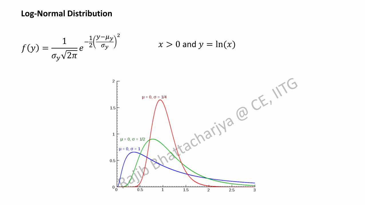
𝑓 𝑦 =1

𝜎𝑦 2𝜋𝑒

−12

𝑦−𝜇𝑦

𝜎𝑦

2

𝑥 > 0 and 𝑦 = ln(𝑥)

Log-Normal Distribution

25

Extreme value (EV) distributions

• Extreme values – maximum or minimum values of sets of data

• Annual maximum discharge, annual minimum discharge

• When the number of selected extreme values is large, the distribution converges to one of the three forms of EV distributions called Type I, II and III

EV type I distributionIf M1, M2…, Mn be a set of daily rainfall or streamflow, and let X = max(Mi) be the maximum for the year. If Mi are independent and identically distributed, then for large n, X has an extreme value type I or Gumbel distribution.

Distribution of annual maximum stream flow follows an EV1 distribution

-5 0 5 10 15 200

0.02

0.04

0.06

0.08

0.1

0.12

0.14

0.16

0.18

0.2

x

f(x)

=0.5

=1

=1.5

=2.0

=2.5

-5 0 5 10 15 200

0.02

0.04

0.06

0.08

0.1

0.12

0.14

0.16

0.18

0.2

x

f(x)

=1

=2

=3

=4

𝑓 𝑥 =1

𝛽𝑒− 𝑦+𝑒−𝑦

𝑦 =𝑥 − 𝜇

𝛽

𝜇 = 𝑥 − 0.5772𝛽 𝛽 =6𝑆𝑥

𝜋

EV type III distributionIf Wi are the minimum stream flows in different days of the year, let X = min(Wi) be the smallest. X can be described by the EV type III or Weibull distribution.

Distribution of low flows (eg. 7-day min flow) follows EV3 distribution.

0 0.5 1 1.5 2 2.50

0.2

0.4

0.6

0.8

1

1.2

1.4

1.6

1.8

x

f(x)

=1 k=0.5

=1 k=1.0

=1 k=1.5

=1 k=2.0

𝑓 𝑥 =𝑘

𝜆

𝑥

𝜆

𝑘−1

𝑒−

𝑥𝜆

𝑘

𝑥 > 0, 𝜆, 𝑘 > 0

Exponential distribution

Poisson process – a stochastic process in which the number of events occurring in two disjoint subintervals are independent random variables.

In hydrology, the interarrival time (time between stochastic hydrologic events) is described by exponential distribution

x

1 xexf x ;0)(

Interarrival times of polluted runoffs, rainfall intensities, etc are described by exponential distribution.

0 0.2 0.4 0.6 0.8 1 1.2 1.4 1.6 1.8 20

0.5

1

1.5

2

2.5

3

3.5

4

4.5

x

f(x)

=0.5

=1.5

=2.5

=3.5

=4.5

Gamma Distribution• The time taken for a number of events (b) in a Poisson process is described by the gamma

distribution

• Gamma distribution – a distribution of sum of b independent and identical exponentially distributed random variables.

Skewed distributions (eg. hydraulic conductivity) can be represented using gamma without log transformation.

function gamma xex

xfx

;0)(

)(1

Pearson Type III

Named after the statistician Pearson, it is also called three-parameter gamma distribution. A lower bound is introduced through the third parameter (e)

function gamma xex

xfx

;)(

)()(

)(1

e

e e

It is also a skewed distribution first applied in hydrology for describing the pdf of annual maximum flows.

Log-Pearson Type III

If log X follows a Person Type III distribution, then X is said to have a log-Pearson Type III distribution

e

e e

x log yey

xfy

)(

)()(

)(1

32

Frequency analysis for extreme events

5772.06

expexp1

)(

xus

uxuxxf

x

uxxF expexp)(

uxy

Ty

xP(xp wherepxFy

yxF

T

T

11lnln

))1ln(ln)(lnln

)exp(exp)(

If you know T, you can find 𝑦𝑇, and once 𝑦𝑇 is know, 𝑥𝑇 can be computed by

TT yux

Q. Find a flow (or any other event) that has a return period of T years

EV1 pdf and cdf

Define a reduced variable y

33

Example 01

Given annual maxima for 10-minute storms. The mean and standard deviation are 0.649 in and 0.177 in.

Find 5 & 50 year return period 10-minute storms

138.0177.0*66

s

569.0138.0*5772.0649.05772.0 xu

ins

inx

177.0

649.0

5.115

5lnln

1lnln5

T

Ty

inyux 78.05.1*138.0569.055

inx 11.150

34

Normal Distribution2

2

1

2

1)(

x

X exf TT

Tz

s

xxK

szxsKxx TTT

054.2;02.050

1;50 5050 zKpT

Normal distribution

So the frequency factor for the Normal Distribution is the standard normal variate

Example: 50 year return period

𝑃 𝑋 > 𝑥𝑇 =1

𝑇=

𝑥𝑇

∞

𝑓 𝑥 𝑑𝑥

𝑥𝑇𝜇

𝐾𝑇𝜎

𝑤 = 𝑙𝑛1

𝑝2

1/2

0 < 𝑝 ≤ 0.5

𝑧 = 𝑤 −2.515517 + 0.802853𝑤 + 0.010328𝑤2

1 + 1.432788𝑤 + 0.189269𝑤2 + 0.001308𝑤3

36

EV-I (Gumbel) Distribution

uxxF expexp)(

s6 5772.0 xu

1lnln

T

TyT

sT

Tx

T

Tssx

yux TT

1lnln5772.0

6

1lnln

665772.0

1lnln5772.0

6

T

TKT

sKxx TT

37

Example 02

Given annual maximum rainfall, calculate 5-yr storm using frequency factor

1lnln5772.0

6

T

TKT

719.015

5lnln5772.0

6

TK

in 0.78

0.177 0.719 0.649

sKxx TT

Distribution PDF CDF Range Mean

Normal 1

𝜎 2𝜋𝑒

−12

𝑥−𝜇𝜎

2

Or

1

2𝜋𝑒−

𝑧2

2 , 𝑧 =𝑥−𝜇

𝜎

−∞

𝑥1

𝜎 2𝜋𝑒

−12

𝑥−𝜇𝜎

2

𝑑𝑥−∞ ≤ 𝑥 ≤ +∞ 𝜇 and 𝜎

Lognormal𝑦 = ln(𝑥)

1

𝜎𝑦 2𝜋𝑒

−12

𝑥−𝜇𝑦

𝜎𝑦

2

−∞

𝑦1

𝜎𝑦 2𝜋𝑒

−12

𝑥−𝜇𝑦

𝜎𝑦

2

𝑑𝑦−∞ ≤ 𝑦 ≤ +∞0 ≤ 𝑥 ≤ +∞

𝜇𝑦 and 𝜎𝑦

Extreme value Type I𝑦 = (𝑥 − 𝛽)/𝛼

1

𝛼𝑒− 𝑦+𝑒−𝑦 𝑒−𝑒−𝑦 −∞ ≤ 𝑥 ≤ +∞ 𝛽 = 𝑥 − 0.5772𝛼

𝛼 =6𝑆𝑥

𝜋

Extreme value Type III

𝛼𝑥𝛼−1𝛽−𝛼𝑒− 𝑥/𝛽 𝛼 1 − 𝑒− 𝑥/𝛽 𝛼 𝑥 ≥ 0 𝛽Γ 1 + 1/𝛼𝛽 Γ 1 + 2/𝛼

Ex. Annual maximum values of 10 min duration rainfall at some place from 1913 to 1947 are presented in Table below. Develop a model for storm rainfall frequency analysis using Extreme Value Type I distribution and calculate the 5, 10, and 50 year return period maximum values of 10 min rainfall of the area.

Year 1910 1920 1930 1940

0 0.53 0.33 0.34

1 0.76 0.96 0.70

2 0.57 0.94 0.57

3 0.49 0.80 0.80 0.92

4 0.66 0.66 0.62 0.66

5 0.36 0.68 0.71 0.65

6 0.58 0.68 1.11 0.63

7 0.41 0.61 0.64 0.60

8 0.47 0.88 0.52

9 0.74 0.49 0.64

Mean 0.649 SD 0.177

Solution

𝛼 =6𝑠

𝜋=

6 × 0.177

𝜋= 0.138

𝑢 = 𝑥 − 0.5772𝛼 = 0.649 − 0.5772 × 0.138 = 0.569

Ty

xP(xp wherepxFy

yxF

T

T

11lnln

))1ln(ln)(lnln

)exp(exp)(

𝑦𝑇 = −𝑙𝑛 𝑙𝑛 1 −1

5= 1.5

𝑥𝑇 = 𝑢 + 𝛼𝑦𝑇 = 0.569 + 0.138 × 1.5 = 0.78

1lnln5772.0

6

T

TKT

𝐾𝑇 = −6

𝜋0.5772 + 𝑙𝑛 𝑙𝑛

5

5 − 1= 0.719

𝑥𝑇 = 𝑥 + 𝐾𝑇𝑠 = 0.649 + 0.719 × 0.177 = 0.78

LOG – PEARSON TYPE III DISTRIBUTION

𝑦 = log(𝑥)

Calculate mean 𝑦, standard deviation 𝑠𝑦 and the coefficient of skewness 𝐶𝑠

The value of z can be calculated using the procedure described earlier.

Ex. Calculate the 5 and 50 year return period maximum discharge of the Guadalupe River, Texas using lognormal and Log-Pearson Type III distribution.

Year 1930 1940 1950 1960 1970

0 55900 13300 23700 9190

1 58000 12300 55800 9740

2 56000 28400 10800 58500

3 7710 11600 4100 33100

4 12300 8560 5720 25200

5 38500 22000 4950 15000 30200

6 179000 17900 1730 9790 14100

7 17200 46000 25300 70000 54500

8 25400 6970 58300 44300 12700

9 4940 20600 10100 15200

SOLUTION

𝑦 = 4.2743 𝑠𝑦 = 0.4027 𝐶𝑠 = −0.0696

𝐾50 for 𝐶𝑠 = 0 is 2.054

𝑦50 = 𝑦 + 𝐾50𝑠𝑦

= 4.2743 + 2.054 × 0.4027 = 5.101

𝑥50 = 10 5.101 = 126300 𝑐𝑓𝑠

𝑥5 = 41060 𝑐𝑓𝑠

Lognormal Distribution

Log-Pearson Type III Distribution

𝐾50 = 2.054 +2.0 − 2.054

−0.1 − 0−0.0696 − 0 = 2.016

𝑦50 = 𝑦 + 𝐾50𝑠𝑦 = 4.2743 + 2.016 × 0.4027 = 5.0863

𝑥50 = 10 5.0863 = 121990 𝑐𝑓𝑠

𝑥5 = 41170 𝑐𝑓𝑠

PLOTING POSITIONS

Plotting position refers to the probability value assigned to each piece of data to be plotted

𝑃 𝑋 ≥ 𝑥𝑚 =𝑚

𝑛California’s formula

𝑃 𝑋 ≥ 𝑥𝑚 =𝑚 − 1

𝑛Modified formula

𝑃 𝑋 ≥ 𝑥𝑚 =𝑚 − 0.5

𝑛Hazen (1930) formula

𝑃 𝑋 ≥ 𝑥𝑚 =𝑚 − 0.3

𝑛 + 0.4Chegodayev’s formula

𝑃 𝑋 ≥ 𝑥𝑚 =𝑚

𝑛 + 1Weibull formula

𝑃 𝑋 ≥ 𝑥𝑚 =𝑚 − 𝑏

𝑛 + 1 − 2𝑏

𝑏 = 0.5 For Hazen (1930) formula

𝑏 = 0.3 For Chegodayev’s formula

𝑏 = 0 For Weibull formula

𝑏 = 3/8 For Blom’s formula

𝑏 = 1/3 For Tukey’s formula

𝑏 = 0.44 For Gringorten’s formula

Year

Mai

mu

mD

isch

arge

(m

3/s

)

Ran

k

Exce

ed

ence

pro

bab

ility

w z

log(

Q)

Log

Q f

rom

Lo

gno

rmal

d

istr

ibu

tio

n

1936 5069 1 0.022 2.76 2.01 3.70 3.541967 1982 2 0.044 2.50 1.70 3.30 3.411972 1657 3 0.067 2.33 1.50 3.22 3.331958 1651 4 0.089 2.20 1.35 3.22 3.271941 1642 5 0.111 2.10 1.22 3.22 3.221942 1586 6 0.133 2.01 1.11 3.20 3.171940 1583 7 0.156 1.93 1.01 3.20 3.131961 1580 8 0.178 1.86 0.92 3.20 3.101977 1543 9 0.200 1.79 0.84 3.19 3.071947 1303 10 0.222 1.73 0.76 3.11 3.031968 1254 11 0.244 1.68 0.69 3.10 3.001935 1090 12 0.267 1.63 0.62 3.04 2.981973 937 13 0.289 1.58 0.56 2.97 2.951975 855 14 0.311 1.53 0.49 2.93 2.921952 804 15 0.333 1.48 0.43 2.91 2.901938 719 16 0.356 1.44 0.37 2.86 2.881957 716 17 0.378 1.40 0.31 2.86 2.851974 714 18 0.400 1.35 0.25 2.85 2.831960 671 19 0.422 1.31 0.20 2.83 2.81

1945 623 20 0.444 1.27 0.14 2.79 2.781949 583 21 0.467 1.23 0.08 2.77 2.761946 507 22 0.489 1.20 0.03 2.70 2.741937 487 23 0.511 1.16 -0.03 2.69 2.721969 430 24 0.533 1.12 -0.08 2.63 2.691965 425 25 0.556 1.08 -0.14 2.63 2.671976 399 26 0.578 1.05 -0.20 2.60 2.651950 377 27 0.600 1.01 -0.25 2.58 2.621978 360 28 0.622 0.97 -0.31 2.56 2.601944 348 29 0.644 0.94 -0.37 2.54 2.581951 348 30 0.667 0.90 -0.43 2.54 2.551953 328 31 0.689 0.86 -0.49 2.52 2.531962 306 32 0.711 0.83 -0.55 2.49 2.501959 286 33 0.733 0.79 -0.62 2.46 2.481966 277 34 0.756 0.75 -0.68 2.44 2.451971 276 35 0.778 0.71 -0.75 2.44 2.421970 260 36 0.800 0.67 -0.83 2.42 2.391954 242 37 0.822 0.63 -0.91 2.38 2.361943 218 38 0.844 0.58 -0.99 2.34 2.331948 197 39 0.867 0.53 -1.08 2.30 2.291964 162 40 0.889 0.49 -1.19 2.21 2.251955 140 41 0.911 0.43 -1.30 2.15 2.201939 140 42 0.933 0.37 -1.43 2.15 2.151963 116 43 0.956 0.30 -1.60 2.06 2.081956 49 44 0.978 0.21 -1.83 1.69 1.99

1.50

2.00

2.50

3.00

3.50

4.00

0.0020.2020.4020.6020.802

Log(

Q)

Exceedence probability

RELIABILITY OF ANALYSIS

Confidence Limits: Statistical estimate often presented with a range, or confidence interval within which the true value can be expected to lie.

Confidence Level 𝛽

Significant Level 𝛼 𝛼 =1 − 𝛽

2i.e. is 𝛽 = 90%, then 𝛼 = 0.05

For a return period 𝑇, the upper limit 𝑈𝑇,𝛼 and lower limit 𝐿𝑇,𝛼 may be specified as

𝑈𝑇,𝛼 = 𝑦 + 𝑠𝑦𝐾𝑇,𝛼𝑈

𝑈𝑇,𝛼 = 𝑦 + 𝑠𝑦𝐾𝑇,𝛼𝐿

𝐾𝑇,𝛼𝑈 =

𝐾𝑇 + 𝐾𝑇2 − 𝑎𝑏

𝑎𝐾𝑇,𝛼

𝐿 =𝐾𝑇 − 𝐾𝑇

2 − 𝑎𝑏

𝑎

𝑎 = 1 −𝑧𝛼

2

2 𝑛 − 1𝑏 = 𝐾𝑇

2 −𝑧𝛼

2

𝑛

𝑧𝛼 is the standard normal variable with exceedence probability 𝛼

Problem: Determine 90% confidence limits for the 100 year discharge using the following data

Logarithmic mean =3.639, standard deviation = 0.4439, coefficient of skewedness = -0.64 for 16 years of data

𝛽 = 0.9 𝛼 = 0.05

Solution:

𝑧𝛼has the exceedence probability of 0.05. This cumulative probability is 0.95.

𝑧𝛼 = 1.645

Considering log-normal distribution, the 𝐾100 = 1.843

𝑎 = 1 −𝑧𝛼

2

2 𝑛 − 1= 1 −

1.6452

2 16 − 1= 0.909799

𝑏 = 𝐾𝑇2 −

𝑧𝛼2

𝑛= 1.8432 −

1.6452

16= 3.227522

𝐾𝑇,𝛼𝑈 =

𝐾𝑇 + 𝐾𝑇2 − 𝑎𝑏

𝑎=

1.843 + 1.8432 − 𝑎𝑏

𝑎= 2.7714

𝐾𝑇,𝛼𝐿 =

𝐾𝑇 − 𝐾𝑇2 − 𝑎𝑏

𝑎=

1.843 − 1.8432 − 𝑎𝑏

𝑎= 1.2804

𝑈𝑇,𝛼 = 𝑦 + 𝑠𝑦𝐾𝑇,𝛼𝑈 = 3.639 + 0.4439 × 2.7714 = 4.869225

𝐿𝑇,𝛼 = 𝑦 + 𝑠𝑦𝐾𝑇,𝛼𝐿 = 3.639 + 0.4439 × 1.2804 = 4.207211

Testing the Goodness of Fit

𝜒2 test is used to test the goodness of fitting

𝜒2 =

𝑖=1

𝑚𝑛 𝑓𝑠 𝑥𝑖 − 𝑝 𝑥𝑖

2

𝑝 𝑥𝑖Where 𝑚 is the number of interval

𝑛𝑓𝑠 𝑥𝑖 is the observed number of occurrence and 𝑛𝑝 𝑥𝑖 is the corresponding expected number of occurrence in the interval 𝑖.

For describing 𝜒2 test, 𝜒2 probability distribution must be defined

𝑓 𝑥 =1

2𝑘/2Γ 𝑘/2𝑥

𝑘2−1𝑒−𝑥/2

F 𝑥 =1

Γ 𝑘/2𝛾 𝑘/2, 𝑥/2

Degree of freedom 𝑣 = 𝑚 − 𝑝 − 1

Check the goodness of fit on Normal Distribution Interval Range 𝑛𝑖

1 20 1

2 25 2

3 30 6

4 35 14

5 40 11

6 45 16

7 50 10

8 55 5

9 60 3

10 65 1

69

Mean 39.77

SD 9.17

𝐵 =1

21 + 0.196854 𝑧 + 0.115194 𝑧 2 + 0.000344 𝑧 3 + 0.019527 𝑧 4 −4

𝐹 𝑧 = 𝐵 for 𝑧 < 0

𝐹 𝑧 = 1 − 𝐵 for 𝑧 ≥ 0

Interval Range 𝑛𝑖 𝑓𝑠(𝑥𝑖) 𝐹𝑠(𝑥𝑖) 𝑧𝑖 B 𝐹(𝑥𝑖) 𝑝(𝑥𝑖) 𝜒2

1 20 1 0.0145 0.0145 -2.1559 0.0154 0.0154 0.0154 0.004084

2 25 2 0.0290 0.0435 -1.6107 0.0535 0.0535 0.0380 0.147864

3 30 6 0.0870 0.1304 -1.0654 0.1436 0.1436 0.0901 0.007632

4 35 14 0.2029 0.3333 -0.5202 0.3012 0.3012 0.1577 0.895245

5 40 11 0.1594 0.4928 0.0251 0.4901 0.5099 0.2087 0.801553

6 45 16 0.2319 0.7246 0.5703 0.2840 0.7160 0.2061 0.22287

7 50 10 0.1449 0.8696 1.1156 0.1325 0.8675 0.1515 0.01965

8 55 5 0.0725 0.9420 1.6609 0.0482 0.9518 0.0843 0.115501

9 60 3 0.0435 0.9855 2.2061 0.0136 0.9864 0.0346 0.159163

10 65 1 0.0145 1.0000 2.7514 0.0032 0.9968 0.0104 0.108361

69 1 2.481923

Mean 39.77

SD 9.17

Degree of freedom 𝑣 = 𝑚 − 𝑝 − 1 = 10 − 2 − 1 = 7 𝜒7,1−0.952 = 14.067

Since 𝜒7,1−0.952 is greater than 𝜒𝑐

2, the null hypothesis can not be rejected

𝑧𝑖 =𝑥𝑖 − 𝜋

𝜎