statistical modeling of extreme values

Statistical Moeling of ExtremeValues: Basic Theory and Its

Implementation in Open SourcePrograming Environment R

Nader TajvidiDepartment of Mathematical Statistics

Lund Institute of TechnologyBox 118

SE-22100 LundSweden

August 6, 2010

Khon Kaen University

Outline

• Some examples of application of extreme valuetheory

• Univariate extreme value distributions

• Characterisation of multivariate extreme valuedistributions

• Bivariate extreme value distributions

• Parametric models for the dependence function

• Parametric and nonparametric estimation of thedependence function

• Monte Carlo approximations to mean integratedsquared errors of parametric and nonparametricestimators

• Application to Australian temperature data

Khon Kaen University August 6, 2010

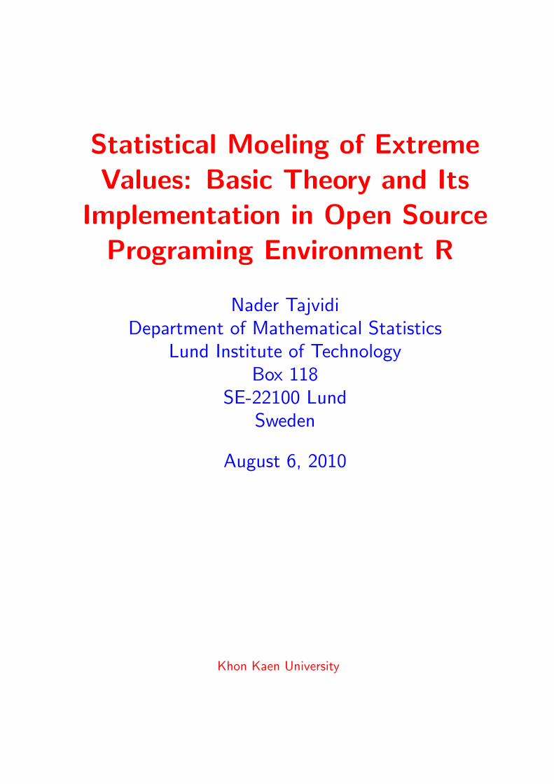
Annualm

axi

mum

sea

leve

lsat

Port

Pirie

,South

Aust

ralia

3.6

3.8

4.0

4.2

4.4

4.6

1930

1940

1950

1960

1970

1980

Yea

r

Sea−Level (meters)

Khon

Kae

nU

niv

ersity

Augu

st6,

2010

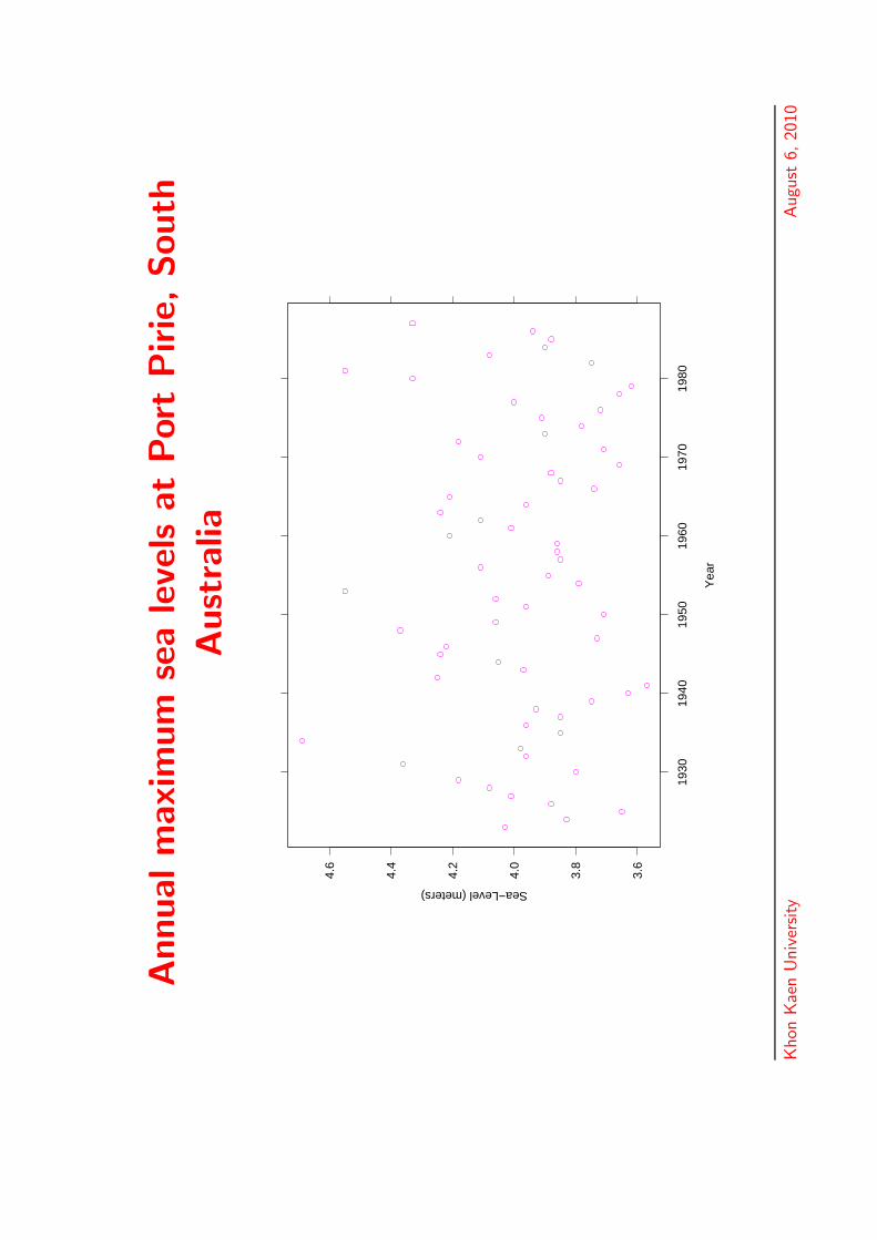
Breaking strengths of glass fibers

0.0

0.5

1.0

1.5

0.5 1.0 1.5 2.0 2.5

Breaking Strength

Den

sity

Density plot of breaking strengths of glass fibers

0

10

20

30

0.5 1.0 1.5 2.0

Breaking Strength

Per

cent

of T

otal

Histogram of breaking strengths of glass fibers


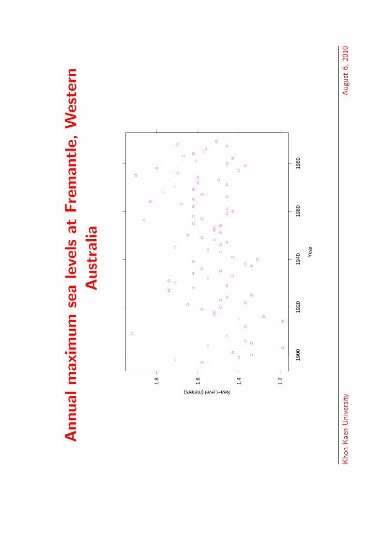
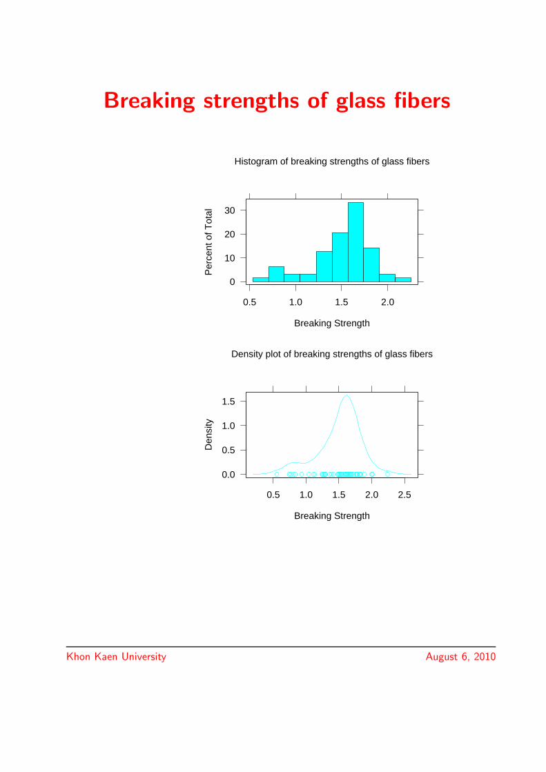
Annualm

axi

mum

sea

leve

lsat

Fre

mantle,

Wes

tern

Aust

ralia

1.2

1.4

1.6

1.8

1900

1920

1940

1960

1980

Yea

r


Khon

Kae

nU

niv

ersity

Augu

st6,

2010

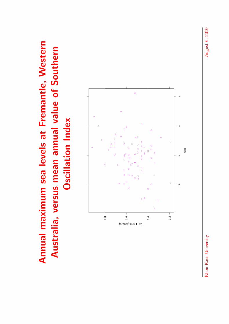
Annualm

axi

mum

sea

leve

lsat

Fre

mantle,

Wes

tern

Aust

ralia

,ve

rsus

mea

nannualva

lue

ofSouth

ern

Osc

illation

Index

1.2

1.4

1.6

1.8

−1

01

2

SO

I


Khon

Kae

nU

niv

ersity

Augu

st6,

2010

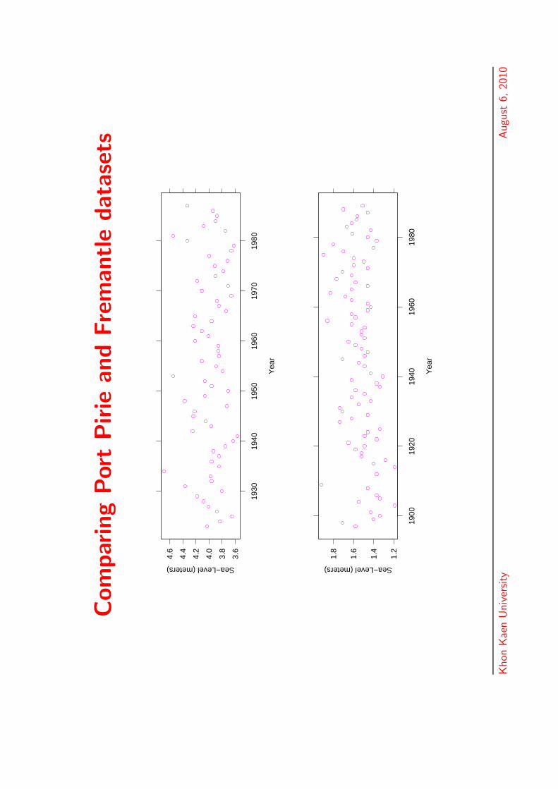
Com

par

ing

Port

Pirie

and

Fre

mantle

data

sets

1.2

1.4

1.6

1.8

1900

1920

1940

1960

1980

Yea

r


3.6

3.8

4.0

4.2

4.4

4.6

1930

1940

1950

1960

1970

1980

Yea

r


Khon

Kae

nU

niv

ersity

Augu

st6,

2010

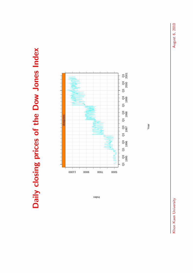
Daily

closing

price

softh

eD

ow

Jones

Index

50007000900011000

Q1

Q3

Q1

Q3

Q1

Q3

Q1

Q3

Q1

Q3

Q1

Q3

Q1

1995

1996

1997

1998

1999

2000

2001

dow

jone

s

Yea

r

Index

Khon

Kae

nU

niv

ersity

Augu

st6,

2010

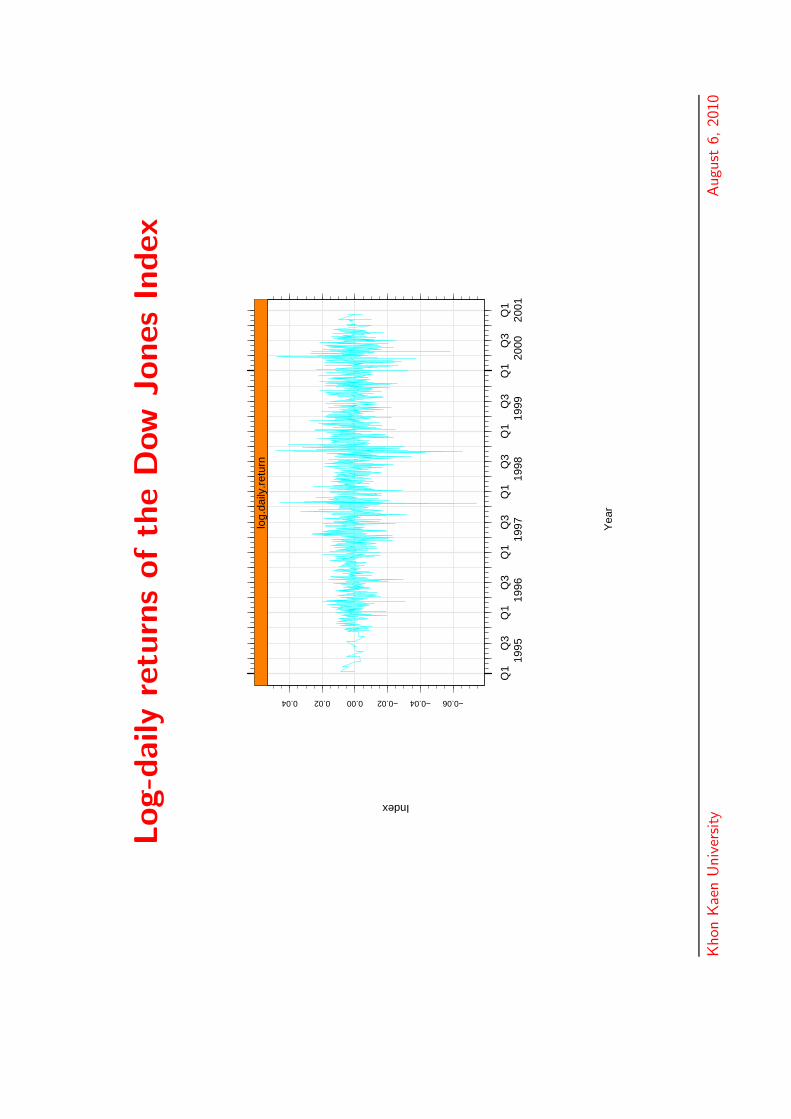
Log-d

aily

retu

rns

ofth

eD

ow

Jones

Index

−0.06−0.04−0.020.000.020.04

Q1

Q3

Q1

Q3

Q1

Q3

Q1

Q3

Q1

Q3

Q1

Q3

Q1

1995

1996

1997

1998

1999

2000

2001

log.

daily

.ret

urn

Yea

r

Index

Khon

Kae

nU

niv

ersity

Augu

st6,

2010

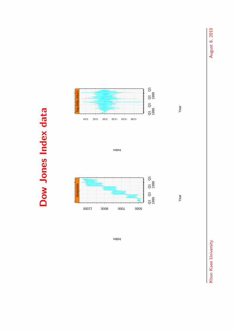
Dow

Jones

Index

data

50007000900011000

Q1

Q1

Q1

Q1

1995

1999

dow

jone

s

Yea

r

Index

−0.06−0.04−0.020.000.020.04

Q1

Q1

Q1

Q1

1995

1999

log.

daily

.ret

urn

Yea

rIndex

Khon

Kae

nU

niv

ersity

Augu

st6,

2010

Windstorm loss data

• Windstorm losses of the Swedish insurance groupLansforsakringar during the period 1982 to 1993

• The database contains:

– The individual amounts of all claims– The place and time of the claims– The type of the claim

• 46 storm events, with a total claimed amount of510 million Swedish crowns (MSEK)

• Farm insurance comprising of approximately 65% ofthe total amount

• All values were corrected for inflation

• No adjustments for portfolio changes


Windstorm losses 1982-1993

Feb 92

Dec 88

Jan 84

Jan

83

Jan 93

Questions:

• How can we predict the size of the next very severestorm?

• How much reinsurance does a company need tobuy?


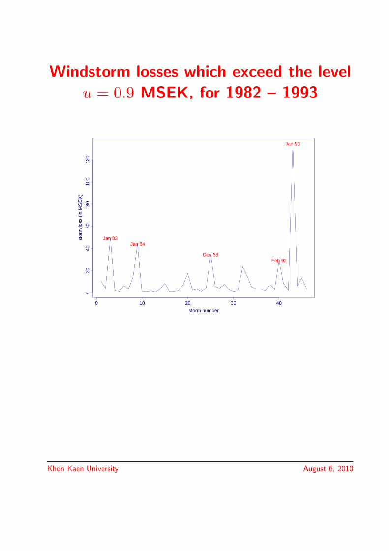
Windstorm losses which exceed the level

u = 0.9 MSEK, for 1982 – 1993

storm number

stor

m lo

ss (

in M

SE

K)

0 10 20 30 40

020

4060

8010

012

0

Jan 83Jan 84

Dec 88Feb 92

Jan 93


Australian temperature data

• A very large dataset on annual maximum andminimum average daily temperatures at 224 stationsacross Australia

QueenslandNew South WalesVictoriaSouth AustraliaWest AustraliaNorthern TerritoryTasmania


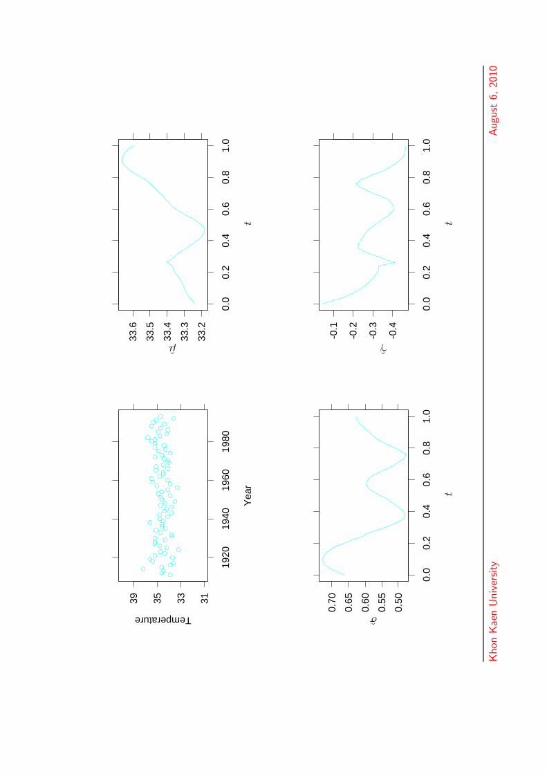
Annual maximum temperatures in

Victoria, Australia

• The maximum value, over all 34 weather stationsthat were operating in the state of Victoria from1910 to 1993, of annual temperatures (in degreesCelsius) during this period.


31333539

1920

1940

1960

1980

Yea

r

Temperature

-0.4

-0.3

-0.2

-0.1

0.0

0.2

0.4

0.6

0.8

1.0

0.50

0.55

0.60

0.65

0.70

0.0

0.2

0.4

0.6

0.8

1.0

33.2

33.3

33.4

33.5

33.6

0.0

0.2

0.4

0.6

0.8

1.0

t

γ

t

σ

t

μ

Khon

Kae

nU

niv

ersity

Augu

st6,

2010

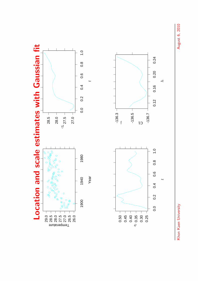
Average annual maximum temperature

• The average annual maximum is derived by takingthe mean of maximum annual temperature readingsat 224 weather stations across Australia in theperiod 1890–1993.



Loca

tion

and

scale

estim

ate

sw

ith

Gauss

ian

fit

26.0

26.5

27.0

27.5

28.0

28.5

29.0

1900

1940

1980

Yea

r

Temperature

27.0

27.5

28.0

28.5

0.0

0.2

0.4

0.6

0.8

1.0

0.25

0.30

0.35

0.40

0.45

0.50

0.0

0.2

0.4

0.6

0.8

1.0

-136

.7

-136

.5

-136

.3

0.12

0.16

0.20

0.24

C1 j

t

μ

t

σ

h

Khon

Kae

nU

niv

ersity

Augu

st6,

2010

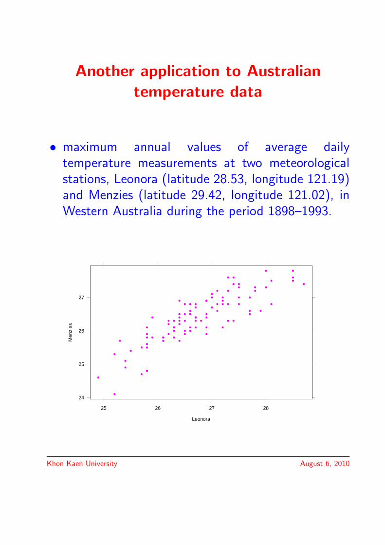
Another application to Australian

temperature data

• maximum annual values of average dailytemperature measurements at two meteorologicalstations, Leonora (latitude 28.53, longitude 121.19)and Menzies (latitude 29.42, longitude 121.02), inWestern Australia during the period 1898–1993.

24

25

26

27

25 26 27 28

Leonora

Men

zies


AnnualM

axi

mum

Win

dSpee

ds

in1944-1

983

50607080

4045

5055

6065

Ann

ual M

axim

um W

ind

Spe

ed (

kont

s) a

t Alb

any

(NY

)

Annual Maximum Wind Speed (konts) at Hartford (CT)

Khon

Kae

nU

niv

ersity

Augu

st6,

2010

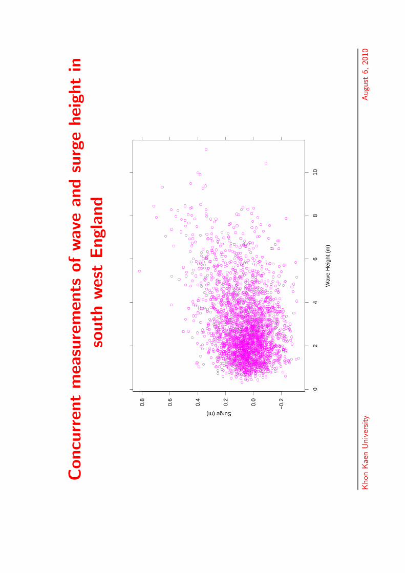
Concu

rren

tm

easu

rem

ents

ofwave

and

surg

ehei

ght

in

south

wes

tEngla

nd

−0.

2

0.0

0.2

0.4

0.6

0.8

02

46

810

Wav

e H

eigh

t (m

)

Surge (m)

Khon

Kae

nU

niv

ersity

Augu

st6,

2010

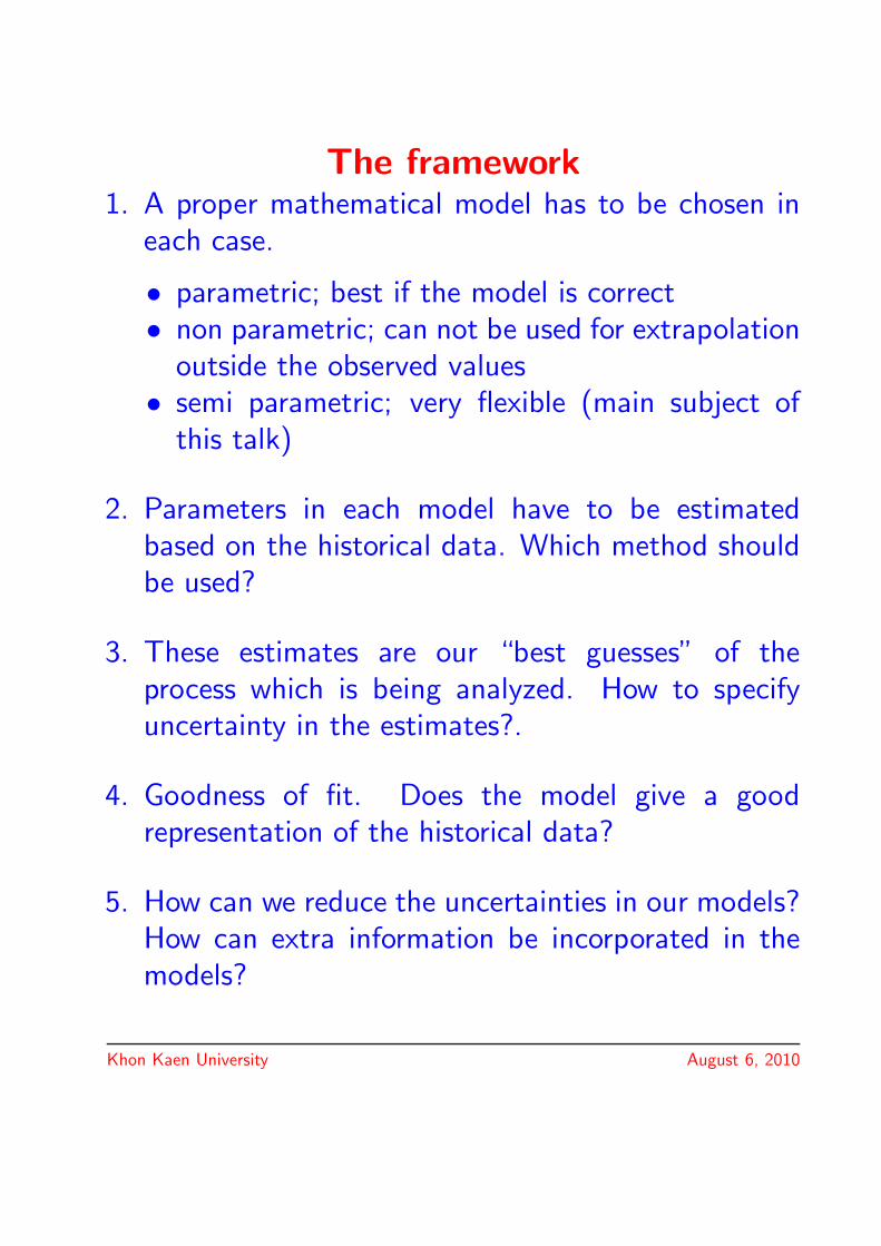
The framework1. A proper mathematical model has to be chosen in

each case.

• parametric; best if the model is correct• non parametric; can not be used for extrapolation

outside the observed values• semi parametric; very flexible (main subject of

this talk)

2. Parameters in each model have to be estimatedbased on the historical data. Which method shouldbe used?

3. These estimates are our “best guesses” of theprocess which is being analyzed. How to specifyuncertainty in the estimates?.

4. Goodness of fit. Does the model give a goodrepresentation of the historical data?

5. How can we reduce the uncertainties in our models?How can extra information be incorporated in themodels?


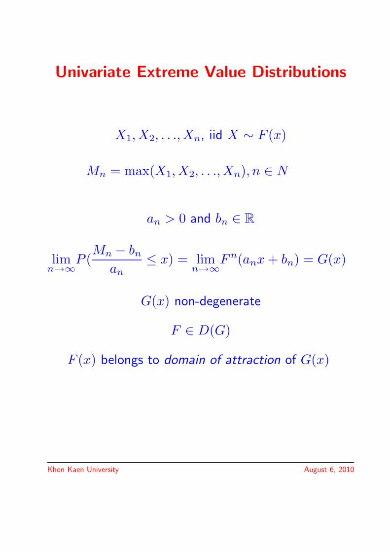
Univariate Extreme Value Distributions

X1,X2, . . .,Xn, iid X ∼ F (x)

Mn = max(X1, X2, . . .,Xn), n ∈ N

an > 0 and bn ∈ R

limn→∞P (

Mn − bn

an≤ x) = lim

n→∞Fn(anx + bn) = G(x)

G(x) non-degenerate

F ∈ D(G)

F (x) belongs to domain of attraction of G(x)


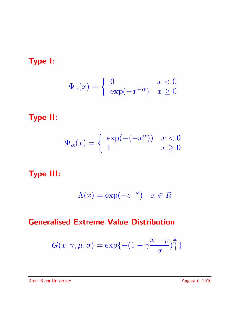
Type I:

Φα(x) ={

0 x < 0exp(−x−α) x ≥ 0

Type II:

Ψα(x) ={

exp(−(−xα)) x < 01 x ≥ 0

Type III:

Λ(x) = exp(−e−x) x ∈ R

Generalised Extreme Value Distribution

G(x; γ, μ, σ) = exp{−(1 − γx − μ

σ)

1γ+}


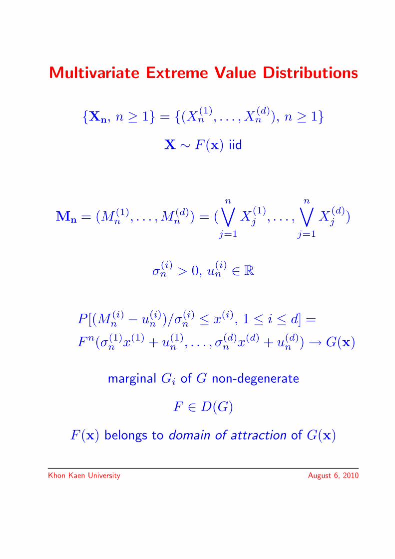
Multivariate Extreme Value Distributions

{Xn, n ≥ 1} = {(X(1)n , . . . , X

(d)n ), n ≥ 1}

X ∼ F (x) iid

Mn = (M (1)n , . . . ,M (d)

n ) = (n∨

j=1

X(1)j , . . . ,

n∨j=1

X(d)j )

σ(i)n > 0, u

(i)n ∈ R

P [(M (i)n − u(i)

n )/σ(i)n ≤ x(i), 1 ≤ i ≤ d] =

Fn(σ(1)n x(1) + u(1)

n , . . . , σ(d)n x(d) + u(d)

n ) → G(x)

marginal Gi of G non-degenerate

F ∈ D(G)

F (x) belongs to domain of attraction of G(x)


Characterisation of Multivariate Extreme

Value Distributions

P [(M (i)n − u(i)

n )/σ(i)n ≤ x(i), 1 ≤ i ≤ d] =

Fn(σ(1)n x(1) + u(1)

n , . . . , σ(d)n x(d) + u(d)

n ) → G(x)

Definition. A df G in Rd is called max-stable if for

every t > 0

Gt(x) = G(α(1)(t)x(1)+β(1)(t), . . . , α(d)(t)x(d)+β(d)(t)).

Definition. A df G in Rd is called max-infinitely

divisible (max-id) if F t(x1, . . . , xd) is a df for everyt > 0.

G(∞,∞, . . . , xi, . . . ,∞) = Φ1(xi) = exp(−x−1i )

G∗(x) is a MEVD with Φ1 marginals


Characterisation of Max-id and

Max-Stable DistributionsF max-id iff for a Radon measure μ on

E := [k,∞] � {k}, k ∈ [−∞,∞)d

F (y) ={

exp{−μ[−∞,y]c} y ≥ k0 otherwise

The measure μ is called an exponent measure.G(∞,∞, . . . , xi, . . . ,∞) = Φ1(xi) = exp(−x−1

i )

G∗(x) is a MEVD with Φ1 marginals if for a finitemeasure S on

ℵ = {y : ‖y‖ = 1}

G∗(x) = exp{−

∫ℵ

d∨i=1

(a(i)

x(i)

)S(da)

}∫ℵ

a(i)S(da) = 1, 1 ≤ i ≤ d


Bivariate Extreme Value Distributions

G∗(x, y) = e−μ∗[0,(x,y)]c

μ∗[0, (x, y)]c = (1x

+1y)A(

x

x + y)

A(w) =∫ 1

0

max{q(1 − w), (1 − q)w}S(dq)

A(w) is called dependence function.

∫ 1

0

qS(dq) =∫ 1

0

(1 − q)S(dq) = 1

• A(0) = A(1) = 1

• max{w, 1 − w} ≤ A(w) ≤ 1

• A(w) is convex for w ∈ [0, 1]


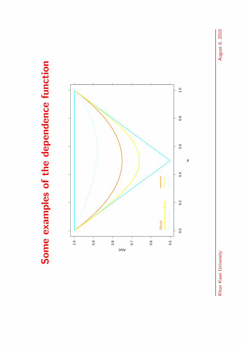
Som

eex

am

ple

softh

edep

enden

cefu

nct

ion

0.5

0.6

0.7

0.8

0.9

1.0

0.0

0.2

0.4

0.6

0.8

1.0

w

A(w)

Mix

edG

ener

alis

ed m

ixed

Asy

m. m

ixed

Khon

Kae

nU

niv

ersity

Augu

st6,

2010

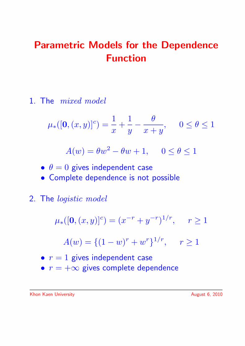
Parametric Models for the Dependence

Function

1. The mixed model

μ∗([0, (x, y)]c) =1x

+1y− θ

x + y, 0 ≤ θ ≤ 1

A(w) = θw2 − θw + 1, 0 ≤ θ ≤ 1

• θ = 0 gives independent case• Complete dependence is not possible

2. The logistic model

μ∗([0, (x, y)]c) = (x−r + y−r)1/r, r ≥ 1

A(w) = {(1 − w)r + wr}1/r, r ≥ 1

• r = 1 gives independent case• r = +∞ gives complete dependence


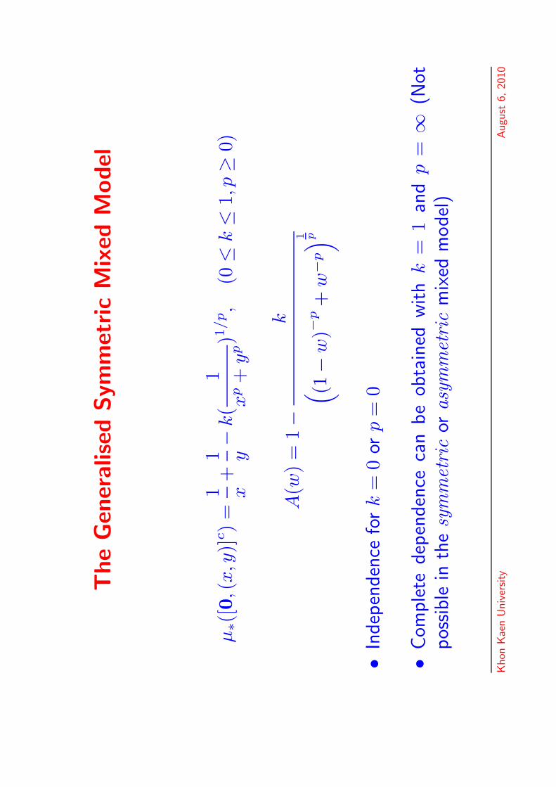
The

Gen

eralis

edSym

met

ric

Mix

edM

odel

μ∗(

[0,(

x,y

)]c)

=1 x

+1 y−

k(

1x

p+

yp)1

/p,

(0≤

k≤

1,p≥

0)

A(w

)=

1−

k( (1

−w

)−p+

w−

p)1 p

•In

dep

enden

cefo

rk

=0

orp

=0

•Com

ple

tedep

enden

ceca

nbe

obta

ined

with

k=

1an

dp

=∞

(Not

pos

sible

inth

esy

mm

etri

cor

asym

met

ric

mix

edm

odel

)

Khon

Kae

nU

niv

ersity

Augu

st6,

2010

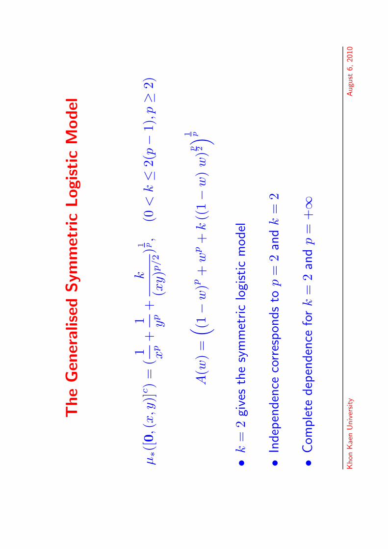
The

Gen

eralis

edSym

met

ric

Logistic

Model

μ∗(

[0,(

x,y

)]c)

=(

1 xp

+1 yp

+k

(xy)p

/2)1 p

,(0

<k≤

2(p−

1),p

≥2)

A(w

)=

( (1−

w)p

+w

p+

k((

1−

w)

w)p 2

)1 p

•k

=2

give

sth

esy

mm

etric

logi

stic

model

•In

dep

enden

ceco

rres

pon

ds

top

=2

and

k=

2

•Com

ple

tedep

enden

cefo

rk

=2

and

p=

+∞

Khon

Kae

nU

niv

ersity

Augu

st6,

2010

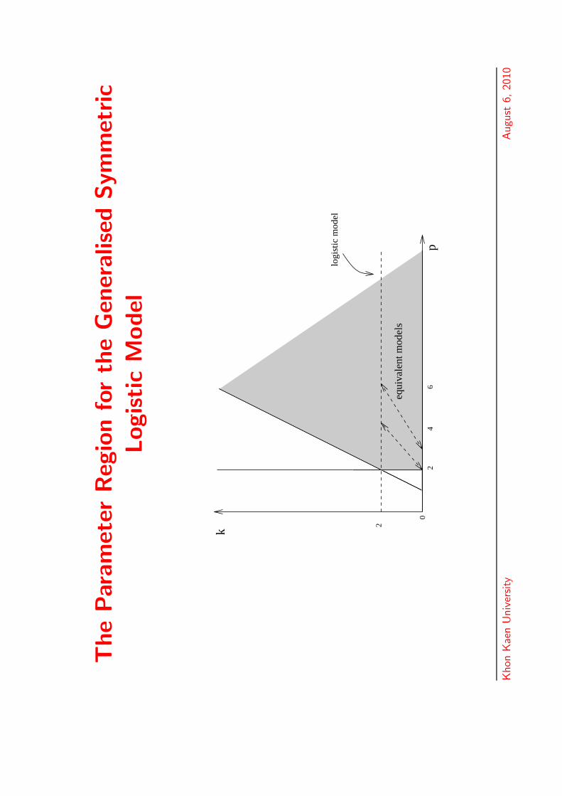
The

Par

am

eter

Reg

ion

for

the

Gen

eralis

edSym

met

ric

Logistic

Model

k

2

2

06

4p

logi

stic

mod

el

equi

vale

nt m

odel

s

Khon

Kae

nU

niv

ersity

Augu

st6,

2010

The

Asy

mm

etric

Mix

edM

odel

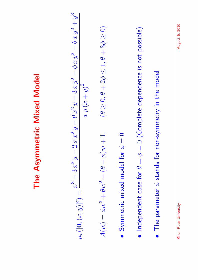
μ∗(

[0,(

x,y

)]c)=

x3+

3x

2y−

2φ

x2y−

θx

2y

+3

xy2−

φx

y2−

θx

y2+

y3

xy

(x+

y)2

A(w

)=

φw

3+

θw2−

(θ+

φ)w

+1,

(θ≥

0,θ

+2φ

≤1,

θ+

3φ≥

0)

•Sym

met

ric

mix

edm

odel

for

φ=

0

•In

dep

enden

tca

sefo

rθ

=φ

=0

(Com

ple

tedep

enden

ceis

not

pos

sible

)

•T

he

par

amet

erφ

stan

ds

for

non

-sym

met

ryin

the

model

Khon

Kae

nU

niv

ersity

Augu

st6,

2010

The

Asy

mm

etric

Logistic

Model

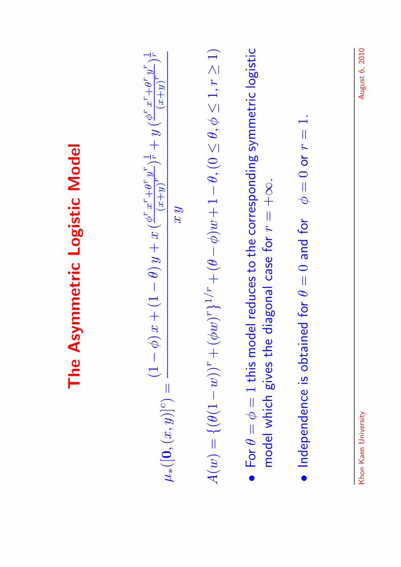
μ∗(

[0,(

x,y

)]c)

=(1

−φ)x

+(1

−θ)

y+

x(φ

rx

r+

θr

yr

(x+

y)r

)1 r+

y(φ

rx

r+

θr

yr

(x+

y)r

)1 r

xy

A(w

)=

{(θ(

1−

w))

r+

(φw

)r}1

/r+

(θ−

φ)w

+1−

θ,(0

≤θ,

φ≤

1,r≥

1)

•For

θ=

φ=

1th

ism

odel

reduce

sto

the

corr

espon

din

gsy

mm

etric

logi

stic

model

whic

hgi

ves

the

dia

gonal

case

for

r=

+∞

.

•In

dep

enden

ceis

obta

ined

for

θ=

0an

dfo

rφ

=0

orr

=1.

Khon

Kae

nU

niv

ersity

Augu

st6,

2010

Estimation of the dependence function

• Nonparametric methods

1. Pickands estimator (1981)2. Caperaa, Fougeres and Genest’s estimator (1997)

• Maximum likelihood based on parametirc models

New Nonparametric Methods:

1. Convex hull of modified Pickands estimator

2. Constrained smoothing splines


Pickands estimator

• Suppose (X,Y ) has a bivariate extreme valuedistribution with exponential margins.

• min{X/(1 − w), Y/w} has an exponentialdistribution with mean 1/A(w).

• the maximum likelihood estimator of A(w) is

An(w) = n

{n∑

i=1

min {Xi/(1 − w), Yi/w}}−1

• For each 0 ≤ w ≤ 1, 1/An(w) is an unbiased andstrongly consistent estimator of 1/A(w).

• δn(w) = n1/2(1/An(w) − 1/A(w)

)satisfies the

central limit theorem in(C(0, 1), B

); see Deheuvels,

P. (1991).


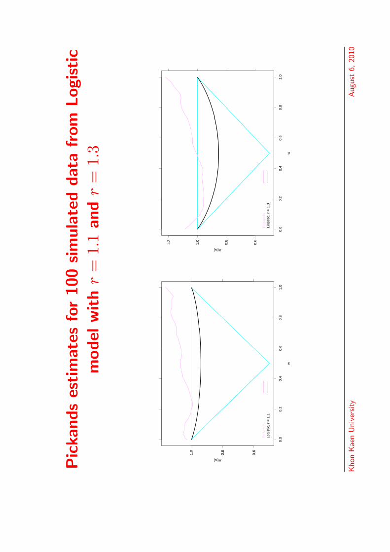
Pic

kands

estim

ate

sfo

r100

sim

ula

ted

data

from

Logistic

model

with

r=

1.1

and

r=

1.3

0.6

0.8

1.0

0.0

0.2

0.4

0.6

0.8

1.0

w

A(w)

Pic

kand

sLo

gist

ic, r

= 1

.1

0.6

0.8

1.0

1.2

0.0

0.2

0.4

0.6

0.8

1.0

w

A(w)

Pic

kand

sLo

gist

ic, r

= 1

.3

Khon

Kae

nU

niv

ersity

Augu

st6,

2010

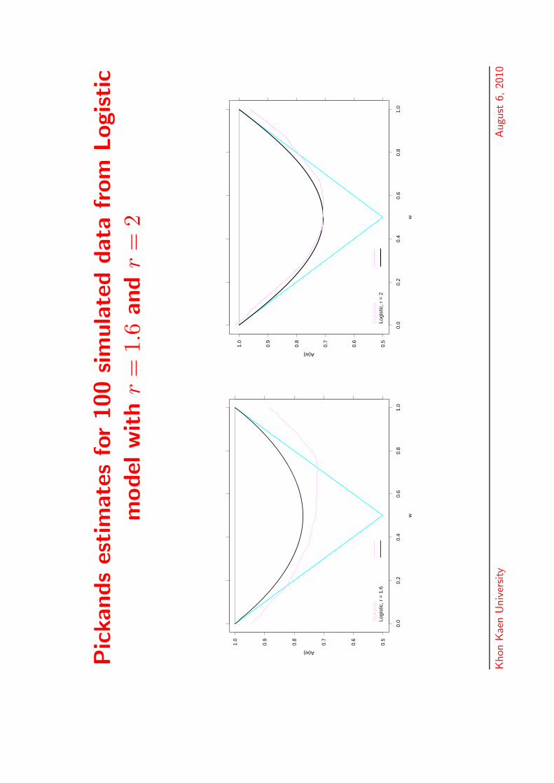
Pic

kands

estim

ate

sfo

r100

sim

ula

ted

data

from

Logistic

model

with

r=

1.6

and

r=

2

0.5

0.6

0.7

0.8

0.9

1.0

0.0

0.2

0.4

0.6

0.8

1.0

w

A(w)

Pic

kand

sLo

gist

ic, r

= 1

.60.

5

0.6

0.7

0.8

0.9

1.0

0.0

0.2

0.4

0.6

0.8

1.0

w

A(w)

Pic

kand

sLo

gist

ic, r

= 2

Khon

Kae

nU

niv

ersity

Augu

st6,

2010

Caperaa, Fougeres and Genest’s

estimator

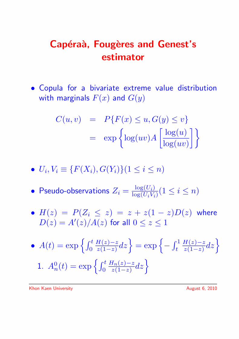
• Copula for a bivariate extreme value distributionwith marginals F (x) and G(y)

C(u, v) = P{F (x) ≤ u,G(y) ≤ v}

= exp{

log(uv)A[

log(u)log(uv)

]}

• Ui, Vi ≡ {F (Xi), G(Yi)}(1 ≤ i ≤ n)

• Pseudo-observations Zi = log(Ui)log(UiVi)

(1 ≤ i ≤ n)

• H(z) = P (Zi ≤ z) = z + z(1 − z)D(z) whereD(z) = A′(z)/A(z) for all 0 ≤ z ≤ 1

• A(t) = exp{∫ t

0H(z)−zz(1−z) dz

}= exp

{− ∫ 1

tH(z)−zz(1−z) dz

}1. A0

n(t) = exp{∫ t

0Hn(z)−zz(1−z) dz

}Khon Kaen University August 6, 2010

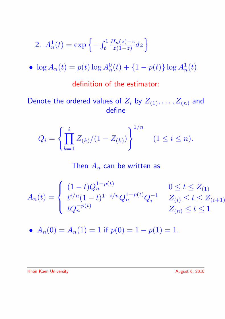
2. A1n(t) = exp

{− ∫ 1

tHn(z)−zz(1−z) dz

}• log An(t) = p(t) log A0

n(t) + {1 − p(t)} log A1n(t)

definition of the estimator:

Denote the ordered values of Zi by Z(1), . . . , Z(n) anddefine

Qi =

{i∏

k=1

Z(k)/(1 − Z(k))

}1/n

(1 ≤ i ≤ n).

Then An can be written as

An(t) =

⎧⎪⎨⎪⎩(1 − t)Q1−p(t)

n 0 ≤ t ≤ Z(1)

ti/n(1 − t)1−i/nQ1−p(t)n Q−1

i Z(i) ≤ t ≤ Z(i+1)

tQ−p(t)n Z(n) ≤ t ≤ 1

• An(0) = An(1) = 1 if p(0) = 1 − p(1) = 1.


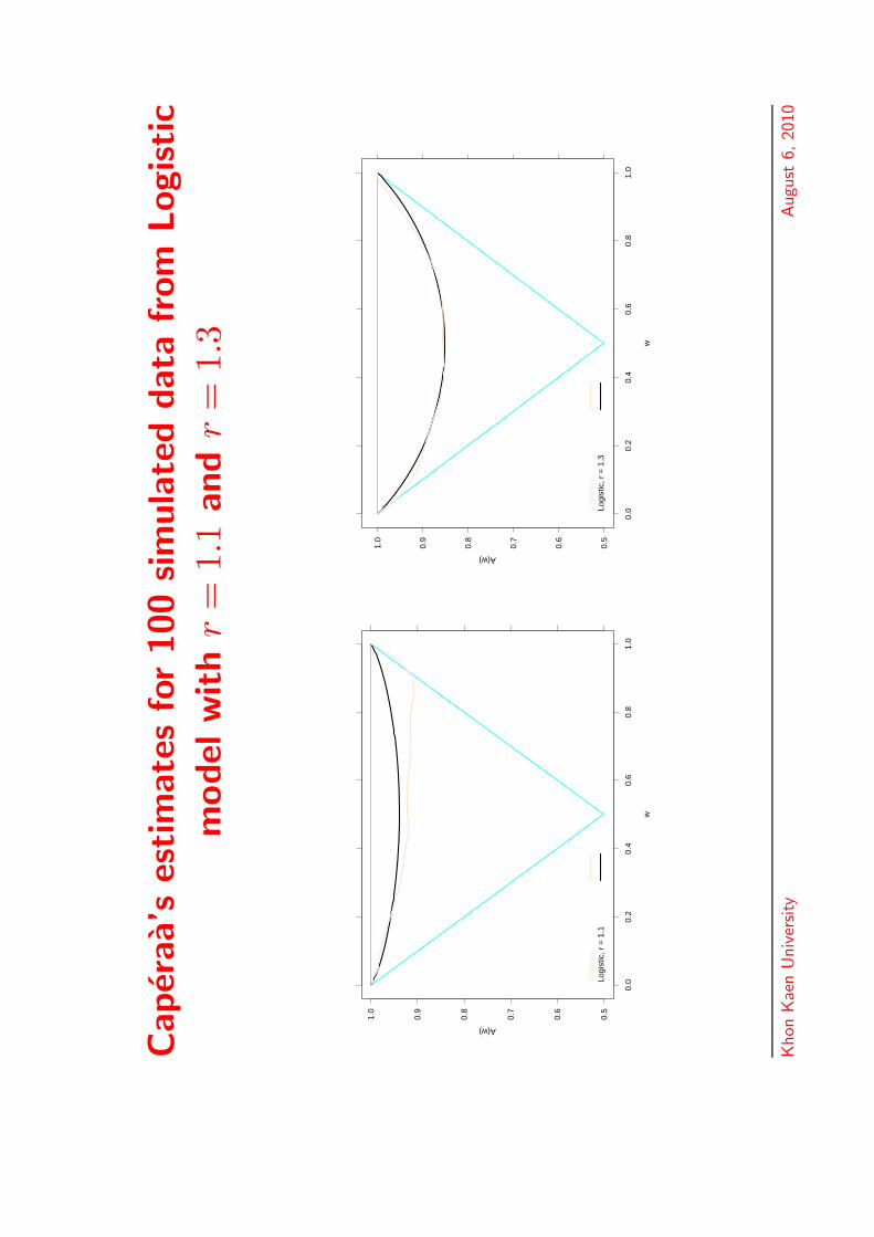
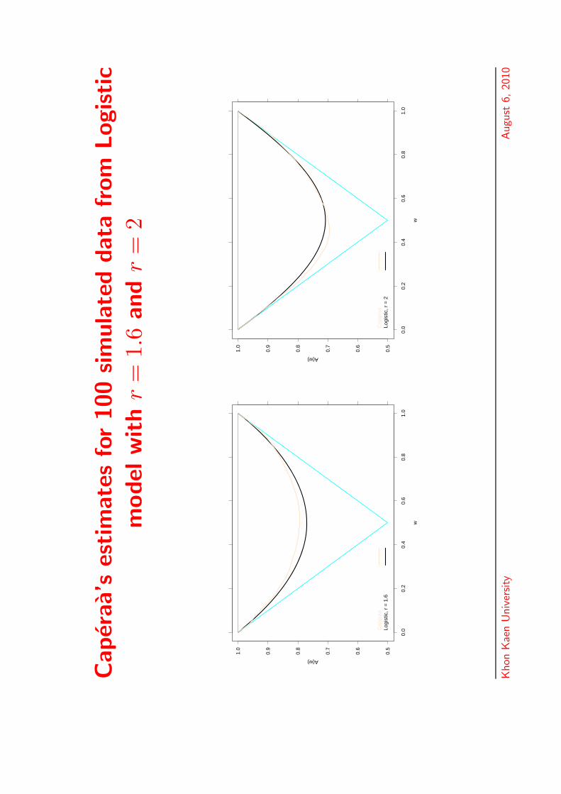
Caper

aa’s

estim

ate

sfo

r100

sim

ula

ted

data

from

Logistic

model

with

r=

1.1

and

r=

1.3

0.5

0.6

0.7

0.8

0.9

1.0

0.0

0.2

0.4

0.6

0.8

1.0

w

A(w)

Cap

eraa

Logi

stic

, r =

1.1

0.5

0.6

0.7

0.8

0.9

1.0

0.0

0.2

0.4

0.6

0.8

1.0

w

A(w)

Cap

eraa

Logi

stic

, r =

1.3

Khon

Kae

nU

niv

ersity

Augu

st6,

2010

Caper

aa’s

estim

ate

sfo

r100

sim

ula

ted

data

from

Logistic

model

with

r=

1.6

and

r=

2

0.5

0.6

0.7

0.8

0.9

1.0

0.0

0.2

0.4

0.6

0.8

1.0

w

A(w)

Cap

eraa

Logi

stic

, r =

1.6

0.5

0.6

0.7

0.8

0.9

1.0

0.0

0.2

0.4

0.6

0.8

1.0

w

A(w)

Cap

eraa

Logi

stic

, r =

2

Khon

Kae

nU

niv

ersity

Augu

st6,

2010

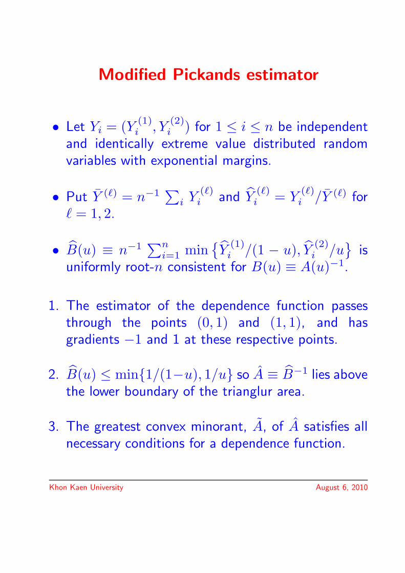
Modified Pickands estimator

• Let Yi = (Y (1)i , Y

(2)i ) for 1 ≤ i ≤ n be independent

and identically extreme value distributed randomvariables with exponential margins.

• Put Y (�) = n−1∑

i Y(�)i and Y

(�)i = Y

(�)i /Y (�) for

= 1, 2.

• B(u) ≡ n−1∑n

i=1 min{Y

(1)i /(1 − u), Y (2)

i /u}

isuniformly root-n consistent for B(u) ≡ A(u)−1.

1. The estimator of the dependence function passesthrough the points (0, 1) and (1, 1), and hasgradients −1 and 1 at these respective points.

2. B(u) ≤ min{1/(1−u), 1/u} so A ≡ B−1 lies abovethe lower boundary of the trianglur area.

3. The greatest convex minorant, A, of A satisfies allnecessary conditions for a dependence function.


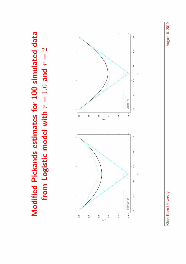
Modifi

edPic

kands

estim

ate

sfo

r100

sim

ula

ted

data

from

Logistic

model

with

r=

1.1

and

r=

1.3

0.5

0.6

0.7

0.8

0.9

1.0

0.0

0.2

0.4

0.6

0.8

1.0

w

A(w)

chul

l of m

odifi

ed P

icka

ndM

odifi

ed P

icka

nds

Logi

stic

, r =

1.1

0.5

0.6

0.7

0.8

0.9

1.0

0.0

0.2

0.4

0.6

0.8

1.0

w

A(w)

chul

l of m

odifi

ed P

icka

ndM

odifi

ed P

icka

nds

Logi

stic

, r =

1.3

Khon

Kae

nU

niv

ersity

Augu

st6,

2010

Modifi

edPic

kands

estim

ate

sfo

r100

sim

ula

ted

data

from

Logistic

model

with

r=

1.6

and

r=

2

0.5

0.6

0.7

0.8

0.9

1.0

0.0

0.2

0.4

0.6

0.8

1.0

w

A(w)

chul

l of m

odifi

ed P

icka

ndM

odifi

ed P

icka

nds

Logi

stic

, r =

1.6

0.5

0.6

0.7

0.8

0.9

1.0

0.0

0.2

0.4

0.6

0.8

1.0

w

A(w)

chul

l of m

odifi

ed P

icka

ndM

odifi

ed P

icka

nds

Logi

stic

, r =

2

Khon

Kae

nU

niv

ersity

Augu

st6,

2010

Constrained smoothing splines

• A may be approximated by a spline that isconstrained to satisfy all the necessary conditionson the dependence function.

• Choose regularly spaced points 0 = t0 < . . . <tm = 1 in the interval [0, 1].

• Given a smoothing parameter s > 0, take As to bea polynomial smoothing spline of degree 3 or morewhich minimises

m∑j=1

{A(tj) − As(tj)}2 + s

∫ 1

0

A′′s(t)2 dt ,

subject to

1. As(0) = As(1) = 12. A′

s(0) ≥ −1 and A′s(1) ≤ 1

3. A′′s ≥ 0 on [0, 1].


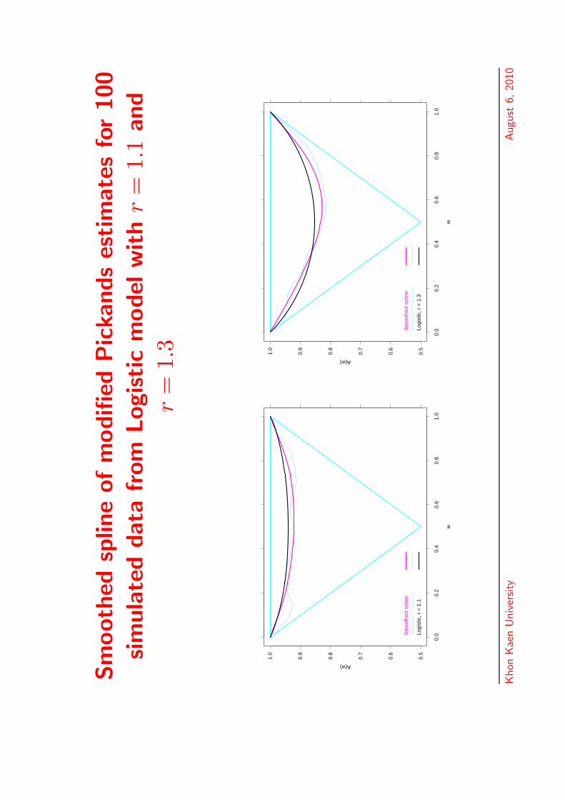
Sm

ooth

edsp

line

ofm

odifi

edPic

kands

estim

ate

sfo

r100

sim

ula

ted

data

from

Logistic

model

with

r=

1.1

and

r=

1.3

0.5

0.6

0.7

0.8

0.9

1.0

0.0

0.2

0.4

0.6

0.8

1.0

w

A(w)

Sm

ooth

ed s

plin

eM

odifi

ed P

icka

nds

Logi

stic

, r =

1.1

0.5

0.6

0.7

0.8

0.9

1.0

0.0

0.2

0.4

0.6

0.8

1.0

w

A(w)

Sm

ooth

ed s

plin

eM

odifi

ed P

icka

nds

Logi

stic

, r =

1.3

Khon

Kae

nU

niv

ersity

Augu

st6,

2010

Sm

ooth

edsp

line

ofm

odifi

edPic

kands

estim

ate

sfo

r100

sim

ula

ted

data

from

Logistic

model

with

r=

1.6

and

r=

2

0.5

0.6

0.7

0.8

0.9

1.0

0.0

0.2

0.4

0.6

0.8

1.0

w

A(w)

Sm

ooth

ed s

plin

eM

odifi

ed P

icka

nds

Logi

stic

, r =

1.6

0.5

0.6

0.7

0.8

0.9

1.0

0.0

0.2

0.4

0.6

0.8

1.0

w

A(w)

Sm

ooth

ed s

plin

eM

odifi

ed P

icka

nds

Logi

stic

, r =

2

Khon

Kae

nU

niv

ersity

Augu

st6,

2010

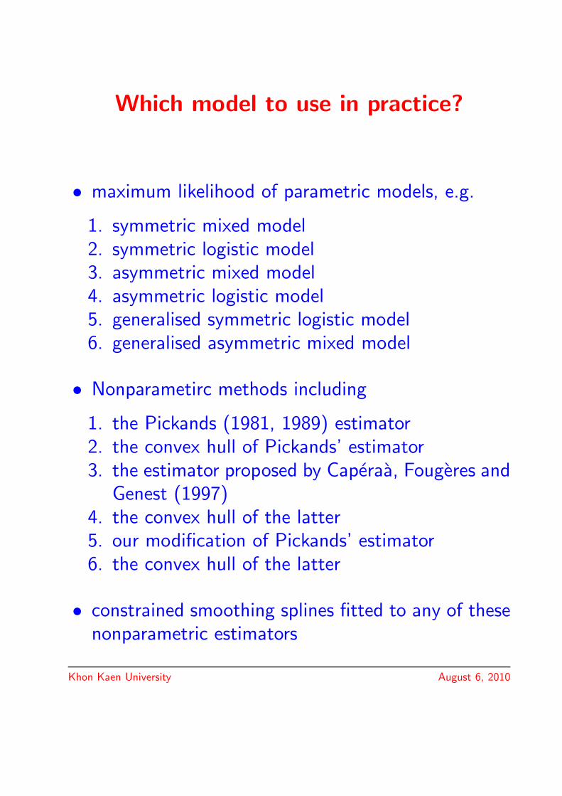
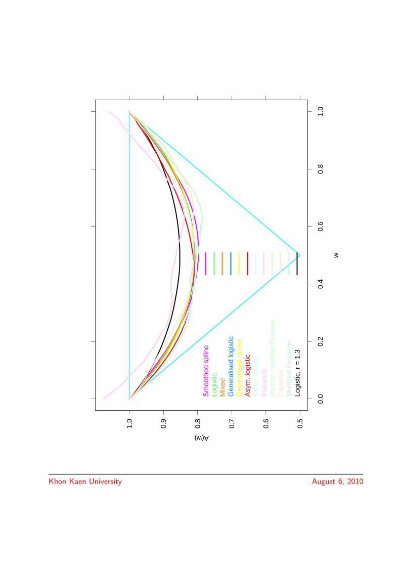
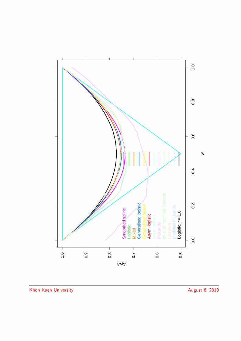
Which model to use in practice?

• maximum likelihood of parametric models, e.g.

1. symmetric mixed model2. symmetric logistic model3. asymmetric mixed model4. asymmetric logistic model5. generalised symmetric logistic model6. generalised asymmetric mixed model

• Nonparametirc methods including

1. the Pickands (1981, 1989) estimator2. the convex hull of Pickands’ estimator3. the estimator proposed by Caperaa, Fougeres and

Genest (1997)4. the convex hull of the latter5. our modification of Pickands’ estimator6. the convex hull of the latter

• constrained smoothing splines fitted to any of thesenonparametric estimators


0.5

0.6

0.7

0.8

0.9

1.0

0.0

0.2

0.4

0.6

0.8

1.0

w

A(w)

Sm

ooth

ed s

plin

eLo

gist

icM

ixed

Gen

eral

ised

logi

stic

Gen

eral

ised

mix

edA

sym

. log

istic

Asy

m. m

ixed

Pic

kand

sch

ull o

f mod

ified

Pic

kand

Cap

eraa

Mod

ified

Pic

kand

sLo

gist

ic, r

= 1

.1


0.5

0.6

0.7

0.8

0.9

1.0

0.0

0.2

0.4

0.6

0.8

1.0

w

A(w)

Sm

ooth

ed s

plin

eLo

gist

icM

ixed

Gen

eral

ised

logi

stic

Gen

eral

ised

mix

edA

sym

. log

istic

Asy

m. m

ixed

Pic

kand

sch

ull o

f mod

ified

Pic

kand

Cap

eraa

Mod

ified

Pic

kand

sLo

gist

ic, r

= 1

.3


0.5

0.6

0.7

0.8

0.9

1.0

0.0

0.2

0.4

0.6

0.8

1.0

w

A(w)

Sm

ooth

ed s

plin

eLo

gist

icM

ixed

Gen

eral

ised

logi

stic

Gen

eral

ised

mix

edA

sym

. log

istic

Asy

m. m

ixed

Pic

kand

sch

ull o

f mod

ified

Pic

kand

Cap

eraa

Mod

ified

Pic

kand

sLo

gist

ic, r

= 1

.6


0.5

0.6

0.7

0.8

0.9

1.0

0.0

0.2

0.4

0.6

0.8

1.0

w

A(w)

Sm

ooth

ed s

plin

eLo

gist

icM

ixed

Gen

eral

ised

logi

stic

Gen

eral

ised

mix

edA

sym

. log

istic

Asy

m. m

ixed

Pic

kand

sch

ull o

f mod

ified

Pic

kand

Cap

eraa

Mod

ified

Pic

kand

sLo

gist

ic, r

= 2


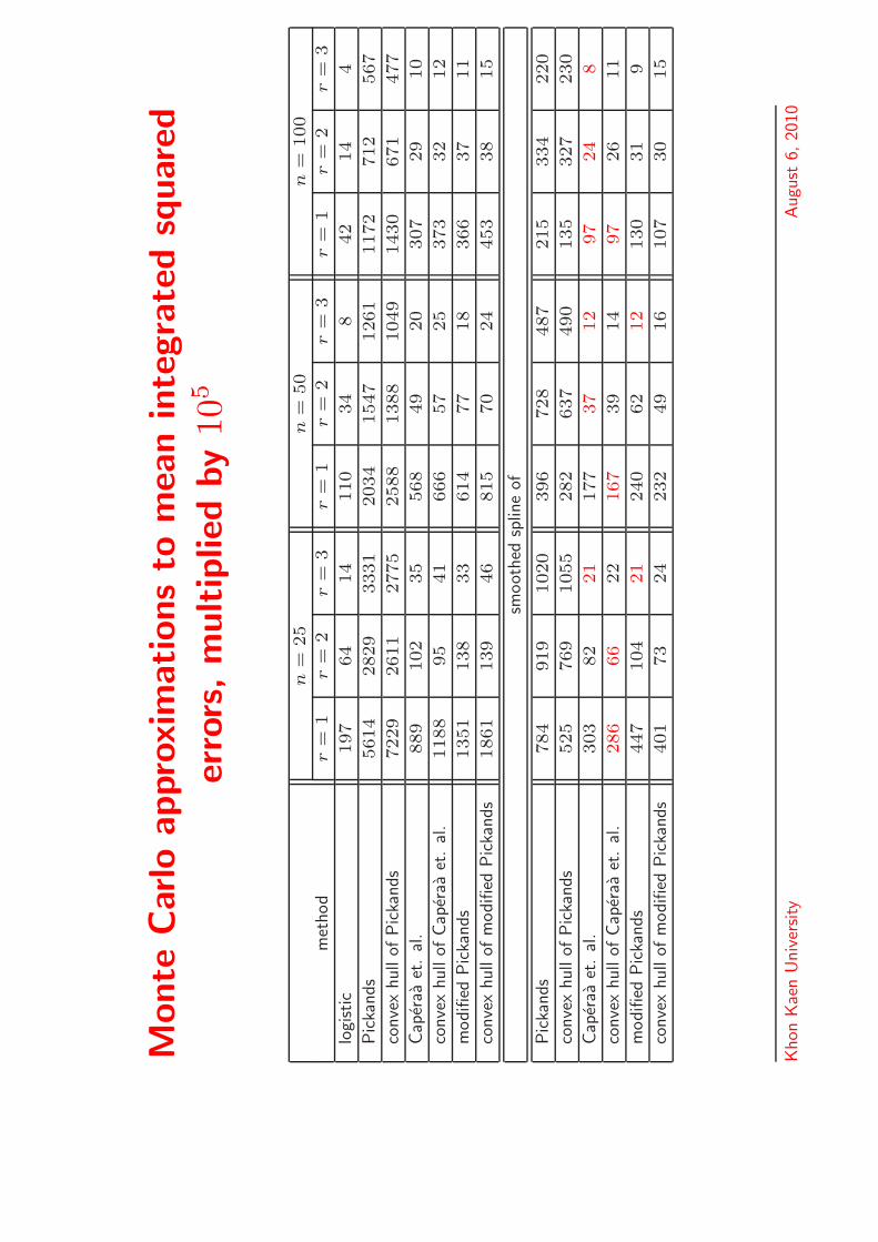
Monte

Car

loappro

xim

ations

tom

ean

inte

gra

ted

squar

ed

erro

rs,m

ultip

lied

by

105

n=

25

n=

50

n=

100

met

hod

r=

1r

=2

r=

3r

=1

r=

2r

=3

r=

1r

=2

r=

3

logi

stic

197

64

14

110

34

842

14

4

Pic

kands

5614

2829

3331

2034

1547

1261

1172

712

567

conve

xhull

ofPic

kands

7229

2611

2775

2588

1388

1049

1430

671

477

Cap

eraa

et.

al.

889

102

35

568

49

20

307

29

10

conve

xhull

ofCap

eraa

et.

al.

1188

95

41

666

57

25

373

32

12

modifi

edPic

kands

1351

138

33

614

77

18

366

37

11

conve

xhull

ofm

odifi

edPic

kands

1861

139

46

815

70

24

453

38

15

smoot

hed

splin

eof

Pic

kands

784

919

1020

396

728

487

215

334

220

conve

xhull

ofPic

kands

525

769

1055

282

637

490

135

327

230

Cap

eraa

et.

al.

303

82

21

177

37

12

97

24

8

conve

xhull

ofCap

eraa

et.

al.

286

66

22

167

39

14

97

26

11

modifi

edPic

kands

447

104

21

240

62

12

130

31

9

conve

xhull

ofm

odifi

edPic

kands

401

73

24

232

49

16

107

30

15

Khon

Kae

nU

niv

ersity

Augu

st6,

2010

Australian temperature data

• A very large dataset on annual maximum andminimum average daily temperatures at 224 stationsacross Australia



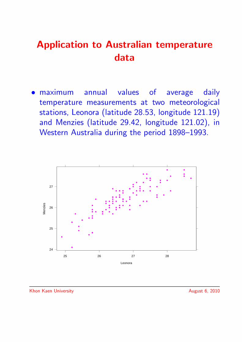
Application to Australian temperature

data

• maximum annual values of average dailytemperature measurements at two meteorologicalstations, Leonora (latitude 28.53, longitude 121.19)and Menzies (latitude 29.42, longitude 121.02), inWestern Australia during the period 1898–1993.

24

25

26

27

25 26 27 28

Leonora

Men

zies


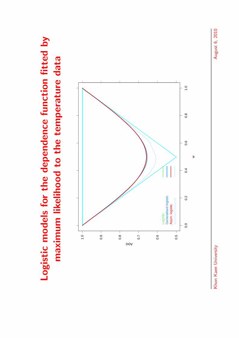
Logistic

model

sfo

rth

edep

enden

cefu

nct

ion

fitt

edby

maxi

mum

likel

ihood

toth

ete

mper

atu

redata

0.5

0.6

0.7

0.8

0.9

1.0

0.0

0.2

0.4

0.6

0.8

1.0

w

A(w)

Logi

stic

Gen

eral

ised

logi

stic

Asy

m. l

ogis

ticM

odifi

ed P

icka

nds

Khon

Kae

nU

niv

ersity

Augu

st6,

2010

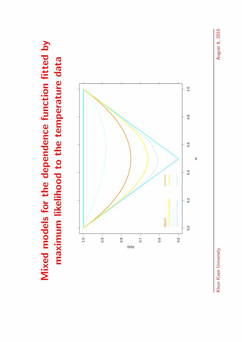
Mix

edm

odel

sfo

rth

edep

enden

cefu

nct

ion

fitt

edby

maxi

mum

likel

ihood

toth

ete

mper

atu

redata

0.5

0.6

0.7

0.8

0.9

1.0

0.0

0.2

0.4

0.6

0.8

1.0

w

A(w)

Mix

edG

ener

alis

ed m

ixed

Asy

m. m

ixed

Mod

ified

Pic

kand

s

Khon

Kae

nU

niv

ersity

Augu

st6,

2010

Estimating a bivariate extreme-value

distribution function

• Let X = (X(1), X(2)) have a bivariate extreme-value distribution F .

• There exist monotone increasing transformationsTj = Tj(·|θj) such that (T1(X(1)), T2(X(2))) hasdistribution function G0.

• Given a sample {Xi = (X(1)i , X

(2)i ), 1 ≤ i ≤ n},

compute a root-n consistent estimator θj of θj from

the marginal data X(j)i , 1 ≤ i ≤ n.

• Put Tj = Tj(·|θj) and

Y(�)j = T�(X

(�)j )

/{n−1

n∑i=1

T�(X(�)i )

}.

• F(x(1), x(2)) = G0

{T1

(x(1)

∣∣θ1

), T2

(x(2)

∣∣θ2

)}is

root-n consistent for F .


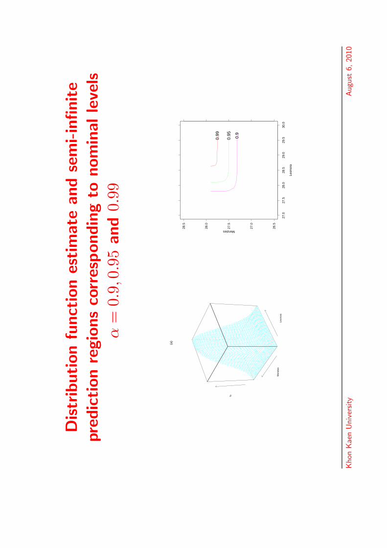
Distr

ibution

funct

ion

estim

ate

and

sem

i-in

finite

pre

dic

tion

regio

ns

corr

espondin

gto

nom

inalle

vels

α=

0.9,

0.95

and

0.99

Leon

ora

Men

zies

fs

(a)

0.9

0.95

0.99

26.5

27.0

27.5

28.0

28.5

27.0

27.5

28.0

28.5

29.0

29.5

30.0

Leon

ora

Menzies

Khon

Kae

nU

niv

ersity

Augu

st6,

2010

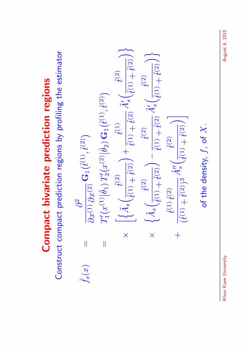
Com

pact

biv

aria

tepre

dic

tion

regio

ns

Con

stru

ctco

mpac

tpr

edic

tion

regi

ons

bypr

ofilin

gth

ees

tim

ator

f s(x

)=

∂2

∂x

(1)∂x

(2)G

1

( t(1) ,

t(2))

=T

′ 1

( x(1

)∣ ∣ θ 1)T′ 2

( x(2

)∣ ∣ θ 2)G1

( t(1) ,

t(2))

×[ { A

s

(t(

2)

t(1)+

t(2)

) +t(

1)

t(1)+

t(2)A

′ s

(t(

2)

t(1)+

t(2)

)}×

{ As

(t(

2)

t(1)+

t(2)

) −t(

2)

t(1)+

t(2)A

′ s

(t(

2)

t(1)+

t(2)

)}+

t(1)t(

2)

(t(1

)+

t(2) )

3A

′′ s

(t(

2)

t(1)+

t(2)

)]of

the

den

sity

,f,of

X.

Khon

Kae

nU

niv

ersity

Augu

st6,

2010

How to choose s

• CV (s) =∫

fs(x)2 dx − 2 n−1∑n

i=1 f−i,s(Xi).

• CV (s) is an almost-unbiased approximation to∫E(f2

s − 2fsf).

• The value of s that results from minimising CV (s)will asymptotically minimise

∫E(fs − f)2.

• To construct prediction regions, define

R(u) ≡ {x : fs(x) ≥ u

}, β(u) =

∫eR(u)

fs(x) dx .

• Given a prediction level α, let u = uα denote thesolution of β(u) = α. Then, R(uα) is a nominalα-level prediction region for a future value of X .


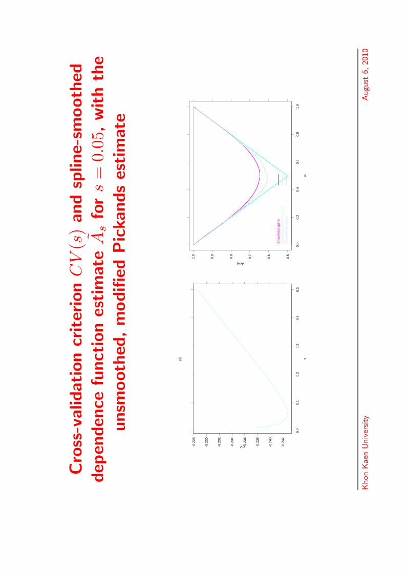
Cro

ss-v

alid

ation

criter

ion

CV

(s)

and

splin

e-sm

ooth

eddep

enden

cefu

nct

ion

estim

ate

As

for

s=

0.05

,w

ith

the

unsm

ooth

ed,m

odifi

edPic

kands

estim

ate

-0.2

42

-0.2

40

-0.2

38

-0.2

36

-0.2

34

-0.2

32

-0.2

30

-0.2

28

0.0

0.1

0.2

0.3

0.4

0.5

s

CV

(a)

0.5

0.6

0.7

0.8

0.9

1.0

0.0

0.2

0.4

0.6

0.8

1.0

wA(w)

Sm

ooth

ed s

plin

ech

ull o

f mod

ified

Pic

kand

Mod

ified

Pic

kand

s

Khon

Kae

nU

niv

ersity

Augu

st6,

2010

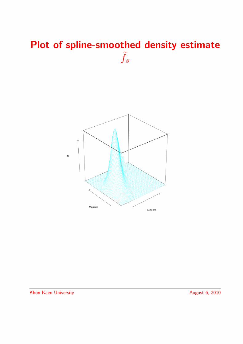
Plot of spline-smoothed density estimate

fs

LeonoraMenzies

fs


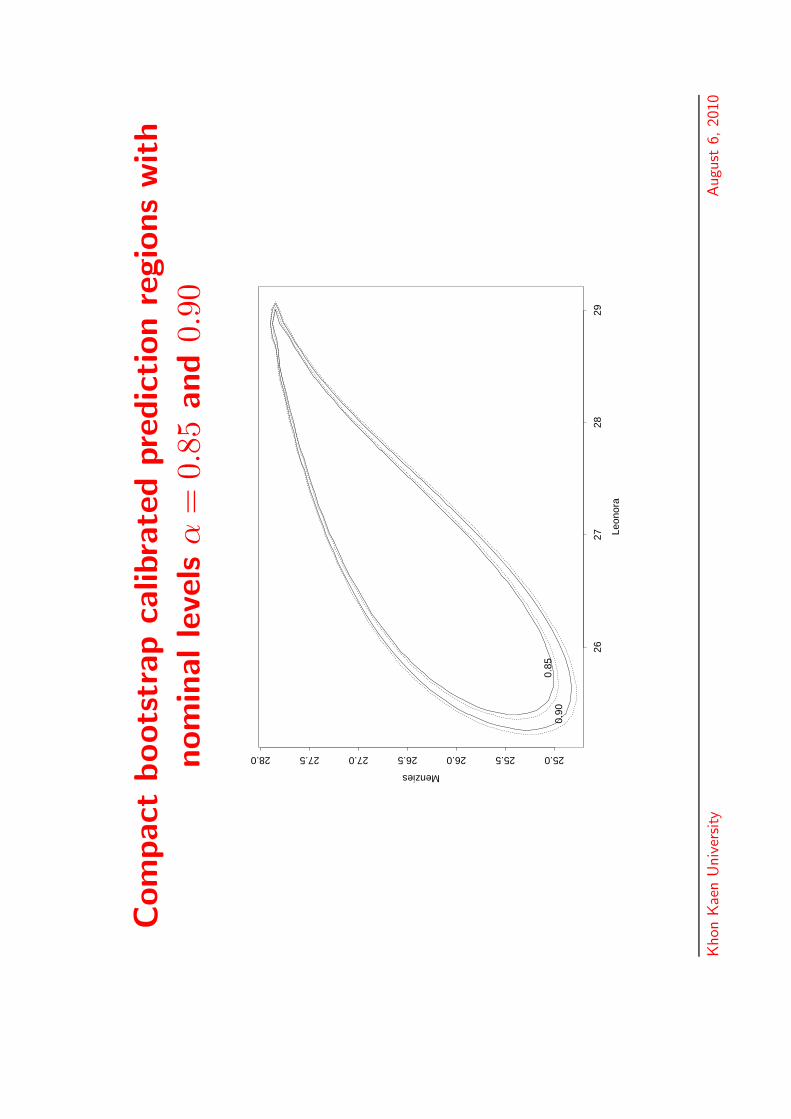
Com

pact

boots

trap

calib

rate

dpre

dic

tion

regio

ns

with

nom

inalle

vels

α=

0.85

and

0.90

Leon

ora

Menzies

2627

2829

25.025.526.026.527.027.528.0

0.85

0.90

Khon

Kae

nU

niv

ersity

Augu

st6,

2010

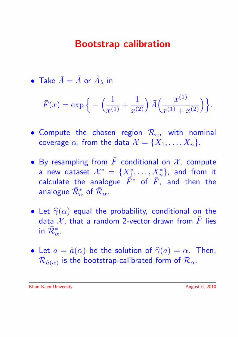
Bootstrap calibration

• Take A = A or Aλ in

F (x) = exp{−

( 1x(1)

+1

x(2)

)A

( x(1)

x(1) + x(2)

)}.

• Compute the chosen region Rα, with nominalcoverage α, from the data X = {X1, . . . ,Xn}.

• By resampling from F conditional on X , computea new dataset X ∗ = {X∗

1 , . . . , X∗n}, and from it

calculate the analogue F ∗ of F , and then theanalogue R∗

α of Rα.

• Let γ(α) equal the probability, conditional on thedata X , that a random 2-vector drawn from F liesin R∗

α.

• Let a = a(α) be the solution of γ(a) = α. Then,Ra(α) is the bootstrap-calibrated form of Rα.


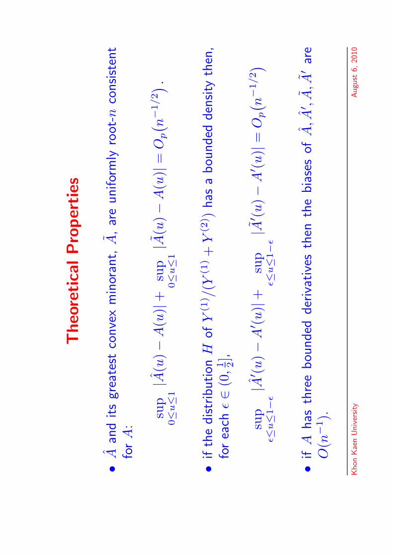
Theo

retica

lPro

per

ties

•A

and

its

grea

test

conve

xm

inor

ant,

A,

are

unifor

mly

root

-nco

nsist

ent

for

A:

sup

0≤

u≤

1|A

(u)−

A(u

)|+

sup

0≤

u≤

1|A

(u)−

A(u

)|=

Op

( n−

1/2) .

•if

the

distr

ibution

Hof

Y(1

) /(Y

(1)+

Y(2

) )has

abou

nded

den

sity

then

,fo

rea

chε∈

(0,1 2],

sup

ε≤u≤

1−

ε|A

′ (u)−

A′ (u)|

+su

pε≤

u≤

1−

ε|A

′ (u)−

A′ (u)|

=O

p

( n−

1/2)

•if

Ahas

thre

ebou

nded

der

ivat

ives

then

the

bia

ses

ofA

,A′ ,

A,A

′ar

eO

(n−

1).

Khon

Kae

nU

niv

ersity

Augu

st6,

2010

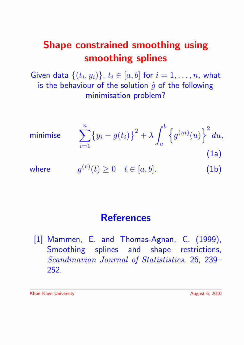
Shape constrained smoothing using

smoothing splines

Given data {(ti, yi)}, ti ∈ [a, b] for i = 1, . . . , n, whatis the behaviour of the solution g of the following

minimisation problem?

minimisen∑

i=1

{yi − g(ti)

}2 + λ

∫ b

a

{g(m)(u)

}2

du,

(1a)

where g(r)(t) ≥ 0 t ∈ [a, b]. (1b)

References

[1] Mammen, E. and Thomas-Agnan, C. (1999),Smoothing splines and shape restrictions,Scandinavian Journal of Statististics, 26, 239–252.


Pro

pose

dEst

imato

rfo

rm

=2

and

r≤

2

For

m=

2,th

epie

cew

ise

pol

ynom

ialre

pres

enta

tion

ofa

nat

ura

lcu

bic

C2-s

plin

eg

is:

g(t

)=

n ∑ i=0

I [t i

,ti+

1)(

t)S

i(t)

,(2

a)

wher

eS

i(t)

=a

i+

b i(t−

t i)+

c i(t−

t i)2

+d

i(t−

t i)3

,1≤

i≤

n−

1,(2

b)

S0(t

)=

a1+

b 1(t−

t 1)

and

Sn(t

)=

Sn−

1(t

n)+

S′ n−

1(t

n)(

t−

t n).

The

coeffi

cien

tsin

(2b)

hav

eto

fulfi

llth

efo

llow

ing

equat

ions

for

gto

be

a

Khon

Kae

nU

niv

ersity

Augu

st6,

2010

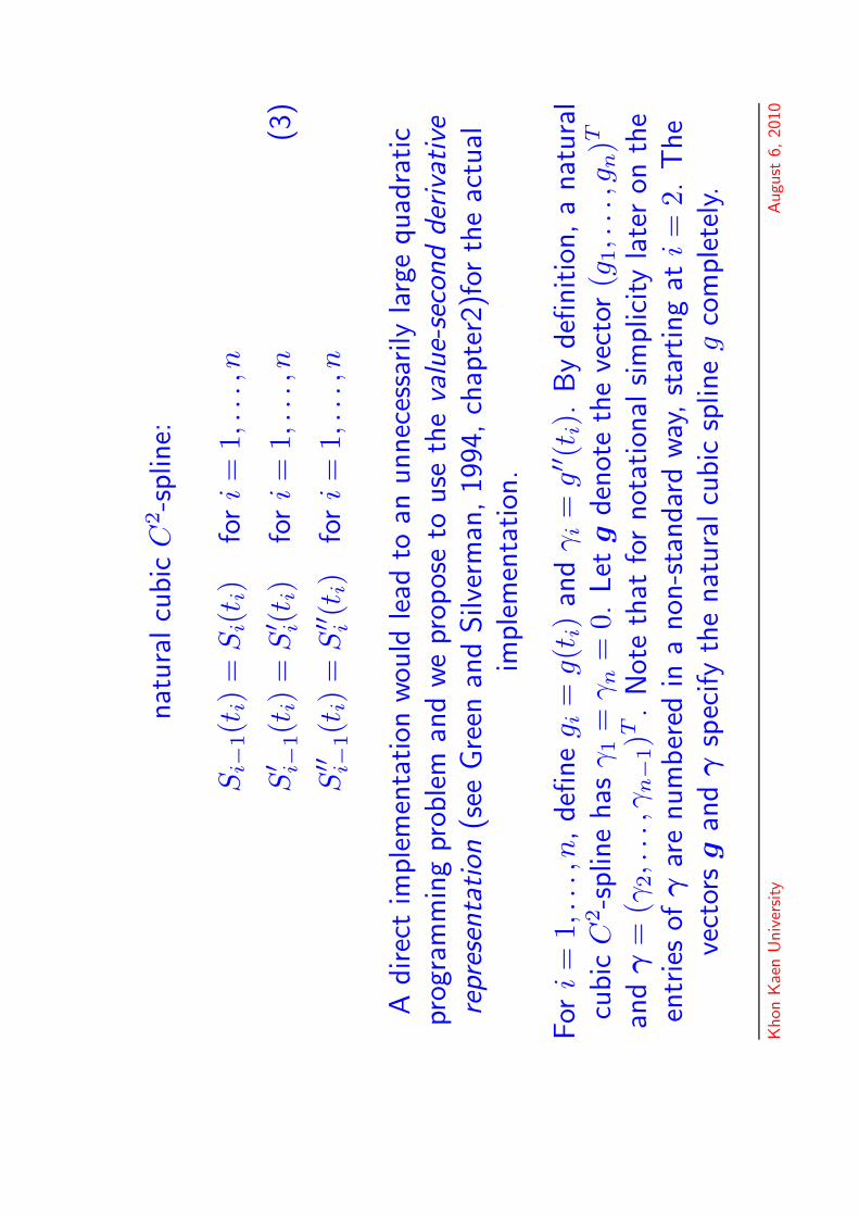
nat

ura

lcu

bic

C2-s

plin

e:

Si−

1(t

i)=

Si(

t i)

for

i=

1,..

.,n

S′ i−

1(t

i)=

S′ i(t i

)fo

ri=

1,..

.,n

(3)

S′′ i−

1(t

i)=

S′′ i(t

i)fo

ri=

1,..

.,n

Adirec

tim

ple

men

tation

wou

ldle

adto

anunnec

essa

rily

larg

equad

ratic

prog

ram

min

gpr

oble

man

dwe

prop

ose

touse

the

valu

e-se

cond

der

ivat

ive

repr

esen

tation

(see

Gre

enan

dSilv

erm

an,19

94,ch

apte

r2)f

orth

eac

tual

imple

men

tation

.

For

i=

1,..

.,n,defi

ne

g i=

g(t

i)an

dγ

i=

g′′ (

t i).

By

defi

nitio

n,a

nat

ura

lcu

bic

C2-s

plin

ehas

γ1

=γ

n=

0.Let

gden

ote

the

vect

or(g

1,.

..,g

n)T

and

γ=

(γ2,.

..,γ

n−

1)T

.N

ote

that

for

not

atio

nal

sim

plic

ity

late

ron

the

entr

ies

ofγ

are

num

ber

edin

anon

-sta

ndar

dway

,st

arting

ati=

2.T

he

vect

ors

gan

dγ

spec

ify

the

nat

ura

lcu

bic

splin

eg

com

ple

tely.

Khon

Kae

nU

niv

ersity

Augu

st6,

2010

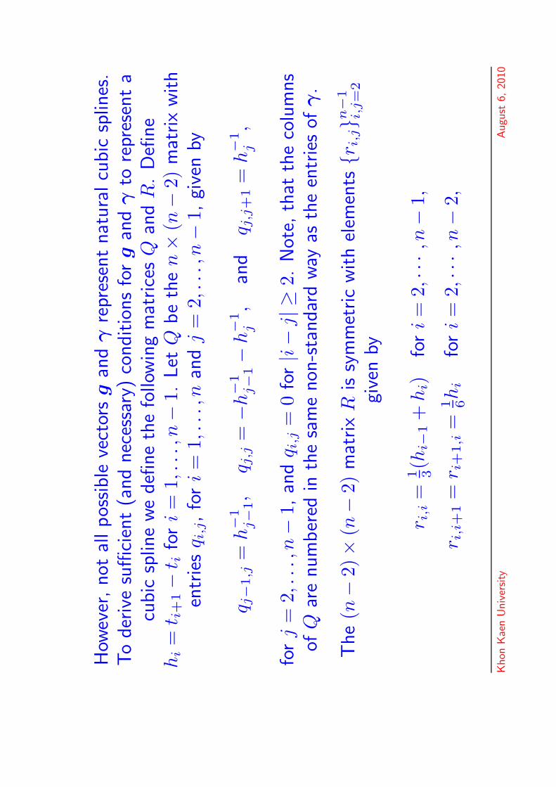
How

ever

,not

allpos

sible

vect

ors

gan

dγ

repr

esen

tnat

ura

lcu

bic

splin

es.

To

der

ive

suffi

cien

t(a

nd

nec

essa

ry)

conditio

ns

for

gan

dγ

tore

pres

ent

acu

bic

splin

ewe

defi

ne

the

follo

win

gm

atrice

sQ

and

R.

Defi

ne

hi=

t i+

1−

t ifo

ri=

1,..

.,n−

1.Let

Qbe

the

n×

(n−

2)m

atrix

with

entr

ies

q i,j,fo

ri=

1,..

.,n

and

j=

2,..

.,n−

1,gi

ven

by

q j−

1,j

=h−

1j−

1,

q j,j

=−h

−1

j−

1−

h−

1j

,an

dq j

,j+

1=

h−

1j

,

for

j=

2,..

.,n−

1,an

dq i

,j=

0fo

r|i−

j|≥

2.N

ote,

that

the

colu

mns

ofQ

are

num

ber

edin

the

sam

enon

-sta

ndar

dway

asth

een

trie

sof

γ.

The

(n−

2)×

(n−

2)m

atrix

Ris

sym

met

ric

with

elem

ents

{ri,

j}n

−1

i,j=

2

give

nby

r i,i

=1 3(h

i−1+

hi)

for

i=

2,···,

n−

1,

r i,i+

1=

r i+

1,i

=1 6h

ifo

ri=

2,···,

n−

2,

Khon

Kae

nU

niv

ersity

Augu

st6,

2010

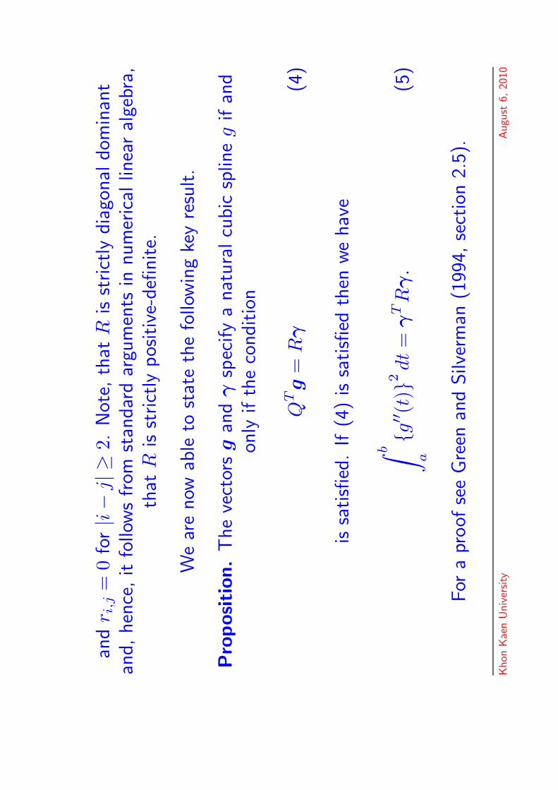
and

r i,j

=0

for|i−

j|≥

2.N

ote,

that

Ris

strict

lydia

gonal

dom

inan

tan

d,hen

ce,it

follo

ws

from

stan

dar

dar

gum

ents

innum

eric

allin

ear

alge

bra,

that

Ris

strict

lypos

itiv

e-defi

nite.

We

are

now

able

tost

ate

the

follo

win

gke

yre

sult.

Pro

position.

The

vect

ors

gan

dγ

spec

ify

anat

ura

lcu

bic

splin

eg

ifan

don

lyif

the

conditio

n

QTg

=R

γ(4

)

issa

tisfi

ed.

If(4

)is

satisfi

edth

enwe

hav

e

∫ b a

{g′′ (

t)}2

dt=

γTR

γ.

(5)

For

apr

oof

see

Gre

enan

dSilv

erm

an(1

994,

sect

ion

2.5)

.

Khon

Kae

nU

niv

ersity

Augu

st6,

2010

This

resu

ltal

low

sus

tost

ate

prob

lem

(1a)

asa

quad

ratic

prog

ram

min

gpr

oble

m.

Let

yden

ote

the

(2n−

2)-v

ecto

r(y

1,.

..,y

n,0

,...

,0)T

,g

the

(2n−

2)-v

ecto

r( g

T,γ

T) T ,

Ath

e(2

n−

2)×

(n−

2)-m

atrix

( Q−R

T) ,

I nth

en×

nunit

mat

rix

and

D=

( I n0

0λR

) .(6

)

Then

the

solu

tion

of(1

a)is

give

nby

the

solu

tion

ofth

efo

llow

ing

quad

ratic

prog

ram

:

min

imise

−y

Tg

+1 2g

TD

g,

(7a)

wher

eA

Tg

=0.

(7b)

We

prop

ose

touse

the

algo

rith

mof

Gol

dfrab

and

Idnan

i(1

982,

1983

)to

solv

e(7

).

Khon

Kae

nU

niv

ersity

Augu

st6,

2010

statistical modeling of extreme values

Documents