pricing algorithms for financial derivatives on baskets ... · pricing algorithms for ﬁnancial...

Pricing Algorithms for financial derivatives onbaskets modeled by Lévy copulas

Christoph Winter, ETH Zurich, Seminar for AppliedMathematics

École Polytechnique, Paris, September 6–8, 2006

Introduction Option pricing Discretization Numerical results Conclusion

Introduction

Option pricingPartial integrodifferential equationVariational formulation

DiscretizationSparse tensor product finite element spaceGalerkin discretizationNumerical quadrature of the Lévy copula kernel

Numerical results

Conclusion

C. Winter École Polytechnique, Paris, September 6–8, 2006 p. 2


LiteratureW. Farkas, N. Reich, C. Schwab, “Anisotropic stable Lévycopula processes – Analytical and numerical aspects.”,Research report No. 2006-08, SAM, ETH Zurich , 2006.

J. Kallsen and P. Tankov, “Characterization of dependence ofmultidimensional Lévy processes using Lévy copulas.”, Journalof Multivariate Analysis, Vol. 97, pp. 1551–1572, (2006).

A.-M. Matache, T. von Petersdorff, C. Schwab, “Fastdeterministic pricing of options on Lévy driven assets.”, M2ANMath. Model. Numer. Anal., Vol. 38, pp. 37–71, (2004).

T. von Petersdorff and C. Schwab, “Numerical solution ofparabolic equations in high dimensions.”, M2AN Math. Model.Numer. Anal., Vol. 38, pp. 93–127, (2004).



Lévy copula and tail integralA function F : R

d→ R is called Lévy copula if

F (u1, . . . ,ud) 6= ∞ for (u1, . . . ,ud) 6= (∞, . . . ,∞),

F (u1, . . . ,ud) = 0 if ui = 0 for at least one i ∈ 1, . . . ,d,

F is d -increasing,

F i(u) = u for any i ∈ 1, . . . ,d, u ∈ R.

The tail integral U : Rd\0 → R

U(x1, . . . , x2) =

d∏

i=1

sgn(xj)ν

d∏

j=1

I(xj)

.



Theorem (Sklar’s theorem for Lévy copulas)For any Lévy process X ∈ R

d exists a Lévy copula F such thatthe tail integrals of X satisfy

U I ((xi )i∈I) = F I ((Ui(xi))i∈I) ,

for any nonempty I ⊂ 1, . . . ,d and any (xi )i∈I ∈ R|I|\0. The

Lévy copula F is unique on∏d

i=1 RanUi .

Lévy density k with marginal Lévy densities k1, . . . , kd ,

k(x1, . . . , xd ) = ∂1 . . . ∂d F |ξ1=U1(x1),...,ξd=Ud (xd )k1(x) . . . kd (x) .



Clayton Lévy copulaIn two dimensions (d=2)

F (u, v) =(|u|−θ + |v |−θ

)− 1θ (η1uv≥0 − (1 − η)1uv≤0

),

(α1, α2)-stable marginal densities

k(x1, x2) = (1 + θ)αθ+11 αθ+1

2 |x1|α1θ−1 |x2|

α2θ−1

·(αθ

1 |x1|α1θ + αθ

2 |x2|α2θ)− 1

θ−2 (

η1x1x2≥0 + (1 − η)1x1x2<0).



Clayton Lévy copula with marginal of CGMY typeCi = 1, Gi = Mi = 4, Yi = 1 for i = 1,2 and η = 1

2Independent θ = 0.5 (left) and dependent θ = 10 (right) tails.



Tempered stable Lévy copula processesLet densities k1, . . . , kd be tempered stable.

With Sklar’s theorem for Lévy copulas there exist a Lévyprocess Xt ∈ R

d with marginal densities k1, . . . , kd .

Log prices are solution of the generalized BS equation

∂u∂t

+ Au = 0 , u|t=T = g ,

where A is the infinitesimal generator of the process Xt withdomain D(A).



Partial integrodifferential equationAssume S i

t = Si0ert+X i

t , 1 ≤ i ≤ d . The price

V (t ,S) = E

(e−r(T−t)g(ST )|St = S

),

is the solution of

∂V∂t

(t ,S) +12

d∑

i ,j=1

SiSjAij∂2V∂Si∂Sj

+ rd∑

i=1

Si∂V∂Si

(t ,S) − rV (t ,S)

+

∫

Rd

(V (t ,Sez) − V (t ,S) −

d∑

i=1

Si (ezi − 1)

∂V∂Si

(t ,S)

)ν(dz) = 0 .

Terminal condition V (T ,S) = g(S).



Transformation to log priceLet xi = log Si , τ = T − t .

∂u∂τ

+ ABS[u] + AJ[u] = 0 ,

with

ABS[ϕ] = −12

d∑

i ,j=1

Aij∂2ϕ

∂xi∂xj+

d∑

i=1

(12

Aii − r)∂ϕ

∂xi+ rϕ ,

AJ[ϕ] = −

∫

Rd

(ϕ(x + z) − ϕ(x) −

d∑

i=1

(ezi − 1)∂ϕ

∂xi(x)

)ν(dz) .

Initial condition

u(0, x) := u0 = g(ex1 , . . . ,exd ) .



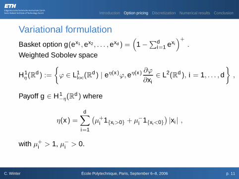
Variational formulation

Basket option g(ex1 ,ex2 , . . . ,exd ) =(

1 −∑d

i=1 exi

)+.

Weighted Sobolev space

H1η (Rd) :=

ϕ ∈ L1

loc(Rd) | eη(x)ϕ,eη(x) ∂ϕ

∂xi∈ L2(Rd ), i = 1, . . . ,d

,

Payoff g ∈ H1−η(R

d ) where

η(x) =

d∑

i=1

(µ+

i 1xi >0 + µ−i 1xi<0)|xi | ,

with µ+i > 1, µ−i > 0.



Bilinear formsWe associate with ABS the bilinear form

aηBS(u, v) =

∫

RdABS[u](x)v(x)e2η(x)

dx ,

and with AJ

aηJ(u, v) =

∫

RdAJ[u](x)v(x)e2η(x)

dx ,

and setaη(u, v) = aη

BS(u, v) + aηJ(u, v) .



Continuity and Gårding inequalityAssume A > 0 and η ∈ L1

loc(Rd) satisfies

(i)∂η

∂xi∈ L∞(Rd ) 1 ≤ i ≤ d ,

(ii) η(x + θz) − η(x) ≤ η(z) ∀x , z ∈ Rd , ∀θ ∈ [0,1] ,

(iii)∫

Rdeη(z) |z| 1|z|>1ν(dz) <∞ .

Then, there exist constants C1, C2, C3 > 0 such that∣∣a−η(u, v)

∣∣ ≤ C1 ‖u‖H1−η(Rd ) ‖v‖H1

−η(Rd ) ,∣∣a−η(u,u)

∣∣ ≥ C2 ‖u‖2H1−η(Rd ) − C3 ‖u‖2

L2−η(Rd ) .



Sparse tensor product finite element spaced=1: Wavelet basis on [−R,R]

VL = spanψ`

j |0 ≤ ` ≤ L, 1 ≤ j ≤ M`

= W0 ⊕ · · · ⊕W` ,

with increment spaces

W0 := V0 , W` := spanψ`

j : 1 ≤ j ≤ M`.

In [−R,R]d

V L := VL ⊗ · · · ⊗ VL =⊕

0≤`i≤L

W`1 ⊗ · · · ⊗W`d .

Sparse tensor product space

V L :=⊕

0≤`1+···+`d≤L

W`1 ⊗ · · · ⊗W`d .



Sparse tensor product space (d = 2)

Difference between V L and V L for level L = 3.



Galerkin discretizationAnsatz

uL(τ, x) =∑

`,j

u`j (τ)ψ

`j (x) .

Linear system

MdU ′(τ) + AdU(τ) = 0 , ∀τ ∈ (0,T ) ,

U(0) = U0 .

Backward Euler time stepping(

Md + ∆tAd)

U(τm) = MdU(τm−1) , m = 1, . . . ,M ,

U(0) = U0 .



Discretized operator (d = 2)We need to compute

aBS(ψ`j , ψ

`′

j ′ ) =d∑

i ,k=1

12

Aik

∫

ΩR

∂ψ`j

∂xi

∂ψ`′

j ′

∂xkdx +

d∑

i=1

12

Aii

∫

ΩR

∂ψ`j

∂xiψ`′

j ′ dx .

In matrix form

A2BS :=

12

A11S ⊗M +12

A22M ⊗S + A12C ⊗(−C)

+12

A11C ⊗M +12

A22M ⊗C .



Discretized operator (d = 2)For the jump part

aJ(ψ`j , ψ

`′

j ′ ) = −

∫

Rd

∫

ΩR

(ψ`

j (x + z)ψ`′

j ′ (x) − ψ`j (x)ψ`′

j ′ (x)

−

d∑

i=1

(ezi − 1)∂ψ`

j

∂xiψ`′

j ′ dx

)ν(dz) .

In matrix form

A2J := −

∫

Rd

(M0,z1 ⊗M0,z2 − M ⊗M

− (ez1 − 1)C ⊗M − (ez2 − 1)M ⊗C

)ν(dz) .



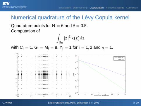
Numerical quadrature of the Lévy Copula kernelQuadrature points for N = 6 and θ = 0.5.Computation of ∫

ΩR

|z|2 k(z)dz

with Ci = 1, Gi = Mi = 8, Yi = 1 for i = 1,2 and η = 1.

−10 −5 0 5 10−10

−8

−6

−4

−2

0

2

4

6

8

10

6 8 10 12 14 16 18 2010

−12

10−10

10−8

10−6

10−4

10−2

100

Number of Refinments

Err

or

theta =0.5theta =10



Operator Matrix (in wavelet basis)For d = 2, L = 5 and R = 5C = (1,1), Y = (1,1), G = (8,8), M = (8,8) and η = 1

2 , θ = 10.

Matrix on full grid (left) and on sparse grid (right).

50 100 150 200 250 300

50

100

150

200

250

300



Comparison stable vs tempered stable processesFor level L = 6.

Matrix for stable processes (left) and tempered stableprocesses (right).

100 200 300 400 500 600 700

100

200

300

400

500

600

700

100 200 300 400 500 600 700

100

200

300

400

500

600

700



Multi-asset optionsLet T = 0.5 and r = 0.

Maximum put options (left) g = (1 − max(S1,S2, . . . ,Sd))+

Basket options (right) g =(

1 −∑d

i=1 Si

)+

0

1

2

00.5

11.5

2

0

0.2

0.4

0.6

0.8

1

SxSy

0

1

2

00.5

11.5

2

0

0.1

0.2

0.3

0.4

0.5

0.6

0.7

0.8

SxSy



Influence of the dependence structureDifference between strong and weak dependence for maximumput option (left) and basket option (right)

0

1

2

00.5

11.5

2

−1

−0.5

0

0.5

1

1.5

2

x 10−3

SxSy

0

1

2

00.5

11.5

2

−10

−5

0

5

x 10−4

SxSy



ConclusionEfficient quadrature rule

Sparse grid technique

Influence of exponential tails on matrix

Influence of dependence structure on option prices


pricing algorithms for financial derivatives on baskets ... · pricing algorithms for ﬁnancial...

Documents