derivatives pricing under collateralization
TRANSCRIPT

Introduction Framework Symmetric Asymmetric Imperfect FBSDE Approximation Scheme Perturbation Technique for Non-linear FBSDEs with Interacting Particle Method
. . . . . . . . . . . . . . . . . . . . .
Numerical Example References
.
.
. ..
.
.
Derivatives Pricing under Collateralization ∗
Masaaki Fujii †, Kenichiro Shiraya ‡, Akihiko Takahashi §
Seminar in Chulalongkorn UniversityFebruary 11, 2013
∗This research is supported by CARF (Center for Advanced Research in Finance) and the global COE program “The research and training
center for new development in mathematics.” All the contents expressed in this research are solely those of the authors and do not represent the
views of any institutions. The authors are not responsible or liable in any manner for any losses and/or damages caused by the use of any contents
in this research.†
Graduate School of Economics, The University of Tokyo‡
Graduate School of Economics, The University of Tokyo§
Speaker, Graduate School of Economics, The University of Tokyo
1 / 114

Introduction Framework Symmetric Asymmetric Imperfect FBSDE Approximation Scheme Perturbation Technique for Non-linear FBSDEs with Interacting Particle Method
. . . . . . . . . . . . . . . . . . . . .
Numerical Example References
Introduction
.
New market realties after the Financial Crisis
.
.
.
. ..
.
.
Wide use of collateralization in OTCDramatic increase in recent years (ISDA Margin Survey 2011)
30%(2003)→ 70%(2010) in terms of trade volume for all OTC.Coverage goes up to 79% (for all OTC) and 88% (for fixed income)among major financial institutions.More than 80% of collateral is Cash.(About half of the cash collateral is USD. )
Persistently wide basis spreads :Much more volatile Cross Currency Swap( CCS) basis
spread.Non-negligible basis spreads even in the single currency
market. (e.g. Tenor swap spread, Libor-OIS spread )
2 / 114

Introduction Framework Symmetric Asymmetric Imperfect FBSDE Approximation Scheme Perturbation Technique for Non-linear FBSDEs with Interacting Particle Method
. . . . . . . . . . . . . . . . . . . . .
Numerical Example References
Source of Funding Cost
Unsecured Funding and Contract (old picture)
Cash
Libor
Loan A B
Cash=PV
option payment
Libor is unsecured offer rate in the interbank market.Libor discounting is appropriate for unsecured trades betweenfinancial firms with Libor credit quality.
3 / 114

Introduction Framework Symmetric Asymmetric Imperfect FBSDE Approximation Scheme Perturbation Technique for Non-linear FBSDEs with Interacting Particle Method
. . . . . . . . . . . . . . . . . . . . .
Numerical Example References
Source of Funding Cost
Collateralized (Secured) Contract (current picture)option payment
cash=pv
collateral
col. rateloan
A B
No outright cash flow (collateral =PV)No external funding is needed.Funding is determined by over-night (ON) rate.⇒ Libor discounting seems inappropriate .
4 / 114

Introduction Framework Symmetric Asymmetric Imperfect FBSDE Approximation Scheme Perturbation Technique for Non-linear FBSDEs with Interacting Particle Method
. . . . . . . . . . . . . . . . . . . . .
Numerical Example References
Important Instruments and Market Realities
Overnight Index Swap (OIS) 1
OIS rate
Compounded ON
Floating side: Daily compounded ON rateMarket Quote : fixed rate, called OIS rate
1Usually, there is only one payment for < 1yr.5 / 114
Introduction Framework Symmetric Asymmetric Imperfect FBSDE Approximation Scheme Perturbation Technique for Non-linear FBSDEs with Interacting Particle Method
. . . . . . . . . . . . . . . . . . . . .
Numerical Example References
Important Instruments and Market Realities
.
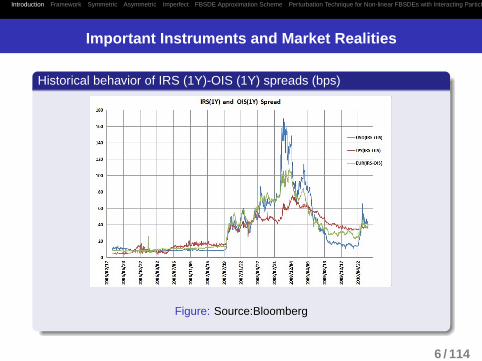
Historical behavior of IRS (1Y)-OIS (1Y) spreads (bps)
.
.
.
. ..
.
.
Figure: Source:Bloomberg
6 / 114

Introduction Framework Symmetric Asymmetric Imperfect FBSDE Approximation Scheme Perturbation Technique for Non-linear FBSDEs with Interacting Particle Method
. . . . . . . . . . . . . . . . . . . . .
Numerical Example References
Important Instruments and Market Realities
Tenor Swap (TS) 2
Libor (short tenor)+spread
Libor (long tenor)
.
.
. ...
.
Spread is quite significant and volatile since late 2007.
2It is also common that payment of short-tenor Leg is compounded and paid at the sametime with the other Leg.
7 / 114

Introduction Framework Symmetric Asymmetric Imperfect FBSDE Approximation Scheme Perturbation Technique for Non-linear FBSDEs with Interacting Particle Method
. . . . . . . . . . . . . . . . . . . . .
Numerical Example References
Important Instruments and Market Realities
.
Historical behavior of JPY TS spreads (bps)
.
.
.
. ..
.
.
Figure: Source:Bloomberg
8 / 114

Introduction Framework Symmetric Asymmetric Imperfect FBSDE Approximation Scheme Perturbation Technique for Non-linear FBSDEs with Interacting Particle Method
. . . . . . . . . . . . . . . . . . . . .
Numerical Example References
Important Instruments and Market Realities
Mark-to-Market Cross Currency Swap
Ni = f(i, j)x (t)
∆ f(i, j)x
N j ≡ 1
Ni ∗ δLi N′i∗ δLi
(N′i= Ni + ∆ f
(i, j)x )
.
.
. ..
.
.
USD Libor is exchanged by Libor +spread of the other currency.
USD leg notional is reset every start of accrual period.
Spread is quite significant and volatile for long time. (it has been changingdrastically and rapidly since the financial crisis.)
9 / 114

Introduction Framework Symmetric Asymmetric Imperfect FBSDE Approximation Scheme Perturbation Technique for Non-linear FBSDEs with Interacting Particle Method
. . . . . . . . . . . . . . . . . . . . .
Numerical Example References
Important Instruments and Market Realities
.
Historical behavior of USDJPY CCS spreads (bps)
.
.
.
. ..
.
.
Figure: Source:Bloomberg
10 / 114

Introduction Framework Symmetric Asymmetric Imperfect FBSDE Approximation Scheme Perturbation Technique for Non-linear FBSDEs with Interacting Particle Method
. . . . . . . . . . . . . . . . . . . . .
Numerical Example References
Important Instruments and Market Realities
.
Historical behavior of EURUSD CCS spreads (bps)
.
.
.
. ..
.
.
Figure: Source:Bloomberg
11 / 114

Introduction Framework Symmetric Asymmetric Imperfect FBSDE Approximation Scheme Perturbation Technique for Non-linear FBSDEs with Interacting Particle Method
. . . . . . . . . . . . . . . . . . . . .
Numerical Example References
Impact of Collateralization
Impact of collateralization :
Reduction of Counter party Exposure
Associated change in CVA has been actively studied.(e.g. CVA is charged for a contract with imperfectcollateralization.)
Change of Funding Cost
Require new term structure model to distinguish discounting andreference rates.Significant impact on derivative pricing.
12 / 114

Introduction Framework Symmetric Asymmetric Imperfect FBSDE Approximation Scheme Perturbation Technique for Non-linear FBSDEs with Interacting Particle Method
. . . . . . . . . . . . . . . . . . . . .
Numerical Example References
Topics of this talk
Valuation framework under collateralization
Perfect collateralizationAsymmetric collateralizationImperfect collateralization and CVA
New approximation scheme for FBSDEs 3 (it seems useful forpricing securities under asymmetric/imperfect collateralization.)
Perturbation schemePerturbation with interacting particle method
Numerical example for CVA and imperfect collateralization
3forward backward stochastic differential equations
13 / 114

Introduction Framework Symmetric Asymmetric Imperfect FBSDE Approximation Scheme Perturbation Technique for Non-linear FBSDEs with Interacting Particle Method
. . . . . . . . . . . . . . . . . . . . .
Numerical Example References
Simple Case: Pricing under Full Collateralization
Assumption
Continuous adjustment of collateral amountSymmetric/Perfect collateralization by CashZero minimum transfer amount
(Daily cash margin call/settlement is becoming popular.)
14 / 114

Introduction Framework Symmetric Asymmetric Imperfect FBSDE Approximation Scheme Perturbation Technique for Non-linear FBSDEs with Interacting Particle Method
. . . . . . . . . . . . . . . . . . . . .
Numerical Example References
Simple Case: Pricing under Full Collateralization
.
.
. ..
.
.
Suppose the payment currency of a European derivative is i, while its collateralcurrency is j. Then, under full collateralization the time- t price of the derivative withpayoff h(i)(T) at maturity T is obtained as follows:
h(i)(t) = EQit
[e−
∫ Tt r(i)(s)ds
(e∫ T
t y( j)(s)ds)
h(i)(T)],
where
y( j)(s) = r( j)(s) − c( j)(s). (2.1)
Qi : risk-neutral measure of currency i
h(i)(T): derivative payoff at time T in currency i
collateral is posted in currency j
c( j)(s): instantaneous collateral rate of currency j at time s
r(i)(s) (r( j)(s)): instantaneous risk-free rate of currency i ( j) at time s
15 / 114

Introduction Framework Symmetric Asymmetric Imperfect FBSDE Approximation Scheme Perturbation Technique for Non-linear FBSDEs with Interacting Particle Method
. . . . . . . . . . . . . . . . . . . . .
Numerical Example References
Simple Case: Pricing under Full Collateralization
Collateral amount in currency j at time s is given by h(i)(s)
f (i, j)x (s)
,
which is invested at the rate of y( j)(s):
h(i)(t) = EQit
[e−
∫ Tt r(i)(s)dsh(i)(T)
]+ f (i, j)
x (t)EQ j
t
∫ T
te−
∫ st r( j)(u)duy( j)(s)
h(i)(s)
f (i, j)x (s)
ds
= EQi
t
[e−
∫ Tt r(i)(s)dsh(i)(T) +
∫ T
te−
∫ st r(i)(u)duy( j)(s)h(i)(s)ds
].
Note that X(t) = e−∫ t0 r(i)(s)dsh(i)(t) +
∫ t
0e−
∫ s0 r(i)(u)duy( j)(s)h(i)(s)ds
is a Qi -martingale. Then, the process of the derivative value is written by
dh(i)(t) =(r(i)(t) − y( j)(t)
)h(i)(t)dt + dM(t)
with some Qi -martingale M . This establishes the proposition.
.
.
. ..
.
.
f (i, j)x (t): Foreign exchange rate at time t(the price of the unit amount of currency ” j”
in terms of currency ” i”).
16 / 114

Introduction Framework Symmetric Asymmetric Imperfect FBSDE Approximation Scheme Perturbation Technique for Non-linear FBSDEs with Interacting Particle Method
. . . . . . . . . . . . . . . . . . . . .
Numerical Example References
Simple Case: Pricing under Full Collateralization
.
Special Case
.
.
.
. ..
.
.
If payment and collateral currencies are the same, the optionvalue is given by
h(t) = EQt
[e−
∫ T
tc(s)dsh(T)
]The discounting is determined by ”collateral rate”, which isconsistent with the schematic picture seen before.
17 / 114

Introduction Framework Symmetric Asymmetric Imperfect FBSDE Approximation Scheme Perturbation Technique for Non-linear FBSDEs with Interacting Particle Method
. . . . . . . . . . . . . . . . . . . . .
Numerical Example References
Setup
Pricing Framework ([ 17])
Filtered probability space (Ω,F , F,Q), where F contains all the marketinformation including defaults.
Consider two firms, i ∈ 1, 2, whose default time is τi ∈ [0,∞], and τ = τ1 ∧ τ2.
τi (and hence τ) is assumed to be totally-inaccessible F-stopping time.
(i.e. a default event is modeled as a jump process.)
Default indicator functions: H it= 1τi≤t(i = 1, 2), H t = 1τ≤t
Assume the existence of absolutely continuous compensator for H i :
Ait=
∫ t
0hi
s1τi>sds, t ≥ 0
Assume no simultaneous defaults, and hence the hazard rate of H is
ht = h1t + h2
t .
Money market account: βt = exp(∫ t
0 rudu)
18 / 114

Introduction Framework Symmetric Asymmetric Imperfect FBSDE Approximation Scheme Perturbation Technique for Non-linear FBSDEs with Interacting Particle Method
. . . . . . . . . . . . . . . . . . . . .
Numerical Example References
Collateralization
When party i ∈ 1, 2 has negative mark-to-market, it has to post cash collateralto party j(, i), and it is assumed to be done continuously.
collateral coverage ratio is δit∈ R+, and the amount of collateral at time t is
given by δit(−V i
t) when party i posts collateral. ( V i
tdenotes the mark-to-market
value of the contract from the view point of party i.)
δit
effectively takes into account under- as well as over -collateralization.Thus, δi
t< 1 and δi
t> 1 are possible.
party j has to pay the collateral rate cit
on the posted cash continuously.
cit
is determined by the currency posted by party i.
market convention is to use overnight (O/N) rate at time t ofcorresponding currency.⇒ Traded through OIS (overnight index swap), which is also collateralized.In general, ci
t, r i
t. (r i
tis the risk-free interest rate of the same currency.)
This is necessary to explain CCS basis spread consistently .
19 / 114

Introduction Framework Symmetric Asymmetric Imperfect FBSDE Approximation Scheme Perturbation Technique for Non-linear FBSDEs with Interacting Particle Method
. . . . . . . . . . . . . . . . . . . . .
Numerical Example References
Counter party Exposure and Recovery Scheme
Counter party exposure to party j at time tfrom the view point of party i is given as:
max(1− δ jt, 0) max(V i
t, 0)+ max(δi
t− 1, 0) max(−V i
t, 0).
Assume party- j’s recovery rate at time t as R jt∈ [0, 1].
Then, the recovery value at the time of j’s default is given as:
R jt
([1 − δ j
t]+[V i
t]+ + [δi
t− 1]+[−V i
t]+
),
x+ ≡ max(x, 0).
20 / 114

Introduction Framework Symmetric Asymmetric Imperfect FBSDE Approximation Scheme Perturbation Technique for Non-linear FBSDEs with Interacting Particle Method
. . . . . . . . . . . . . . . . . . . . .
Numerical Example References
Pricing Formula
• Pricing from the view point of party 1.
St = βt EQ[∫
] t,T]β−1
u 1τ>udDu +
(y1
uδ1u1Su<0 + y2
uδ2u1Su≥0
)Sudu
+
∫] t,T]β−1
u 1τ≥u(Z1(u,Su−)dH1
u + Z2(u,Su−)dH2u
)∣∣∣∣∣∣Ft
]• D: cumulative dividend to party 1.• Default payoff: Z i when party i defaults.
Z1(t, v) =(1− l1t (1− δ
1t )+)v1v<0 +
(1+ l1t (δ
2t − 1)+
)v1v≥0
Z2(t, v) =(1− l2t (1− δ
2t )+)v1v≥0 +
(1+ l2t (δ
1t − 1)+
)v1v<0,
l it≡ (1− Ri
t), i = 1, 2
• yit= r i
t− ci
t, (i ∈ 1, 2) denotes the instantaneous return for j or funding cost for i
at time t from the cash collateral posted by party i.
21 / 114

Introduction Framework Symmetric Asymmetric Imperfect FBSDE Approximation Scheme Perturbation Technique for Non-linear FBSDEs with Interacting Particle Method
. . . . . . . . . . . . . . . . . . . . .
Numerical Example References
Pricing Formula
• (Remark) The return from risky investments, or the borrowing costfrom the external market can be quite different from the risk-freerate, of course.However, if one wants to treat this fact directly, an explicit modelingof the associated risks is required.Here, we use the risk-free rate as net return/cost after hedging theserisks .As we shall see, under full collateralization the final formula doesnot require any knowledge of the risk-free rate , and hence there isno need of its estimation.
22 / 114

Introduction Framework Symmetric Asymmetric Imperfect FBSDE Approximation Scheme Perturbation Technique for Non-linear FBSDEs with Interacting Particle Method
. . . . . . . . . . . . . . . . . . . . .
Numerical Example References
Pricing Formula
Following the method in Duffie&Huang (1996), the pre-default value of thecontract Vt such that Vt1τ>t = St is given by
Vt = EQ[∫
] t,T]exp
(−
∫ s
t
(ru − µ(u,Vu)
)du
)dDs
∣∣∣∣∣∣Ft
], t ≤ T,
where
µ(t, v) = y1t 1v<0 + y2
t 1v≥0 (adjusted term of the discount rate)
yit= δi
tyi
t− (1− δi
t)+(l i
thi
t) + (δi
t− 1)+(l j
th j
t),
if some technical condition(so called no jump condition for V at default) 4 is
satisfied, which is assumed hereafter.(for instance, r, D, yi , δi , l i and hi ,
(i = 1, 2) are adapted to background filtration. In particular, we limit our
attention to the intensities conditional on no-default.)
4This technical condition (∆Vτ = 0) becomes important when we consider creditderivatives: the condition is violated in general when the contagious effects induce jumps tovariables contained in pre-default value process. (e.g. Schonbucher(2000),Collin-Dufresne-Goldstein-Hugonnier(2004), Brigo-Capponi(2009), [19])
23 / 114

Introduction Framework Symmetric Asymmetric Imperfect FBSDE Approximation Scheme Perturbation Technique for Non-linear FBSDEs with Interacting Particle Method
. . . . . . . . . . . . . . . . . . . . .
Numerical Example References
Symmetric Case
Effective discount factor is non-linear :
r t − µ(t, v) = r t − (y1t 1v<0 + y2
t 1v≥0),
which makes the portfolio value non-additive .If y1
t= y2
t= yt , then we have
µ(t, v) = yt .
Further, if y is not explicitly dependent on V, we can recover the linearity.
Vt = EQ
[∫] t,T]
exp(−
∫ s
t(ru − yu)du
)dDs
∣∣∣∣∣∣Ft
]Portfolio valuation can be decomposed into that of each payment.
⇓A good characteristic for market benchmark price.
24 / 114

Introduction Framework Symmetric Asymmetric Imperfect FBSDE Approximation Scheme Perturbation Technique for Non-linear FBSDEs with Interacting Particle Method
. . . . . . . . . . . . . . . . . . . . .
Numerical Example References
Symmetric Perfect Collateralization
.
Special Cases
.
.
.
. ..
.
.
Case 1 : Benchmark for single currency product
bilateral perfect collateralization (δ1 = δ2 = 1)
both parties use the same currency (i) as collateral, which is also thepayment (evaluation) currency.
V(i)t= EQ(i)
[∫] t,T]
exp(−
∫ s
tc(i)
u du)
dDs
∣∣∣∣∣∣Ft
]
The valuation method for single currency swap adopted by LCHSwapclear (2010) is the same with this equation. 5
5See also Piterbarg (2010) for other derivation of this equation.
25 / 114
Introduction Framework Symmetric Asymmetric Imperfect FBSDE Approximation Scheme Perturbation Technique for Non-linear FBSDEs with Interacting Particle Method
. . . . . . . . . . . . . . . . . . . . .
Numerical Example References
Symmetric Perfect Collateralization
.
Special Cases
.
.
.
. ..
.
.
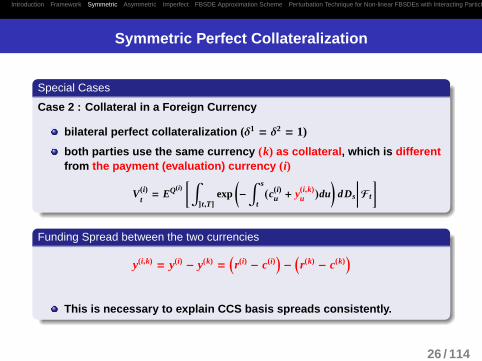
Case 2 : Collateral in a Foreign Currency
bilateral perfect collateralization (δ1 = δ2 = 1)
both parties use the same currency (k) as collateral , which is differentfrom the payment (evaluation) currency (i)
V(i)t= EQ(i)
[∫] t,T]
exp(−
∫ s
t
(c(i)
u + y(i,k)u
)du
)dDs
∣∣∣∣∣∣Ft
]
.
Funding Spread between the two currencies
.
.
.
. ..
.
.
y(i,k) = y(i) − y(k) =(r(i) − c(i)
)−
(r(k) − c(k)
)
This is necessary to explain CCS basis spreads consistently.
26 / 114

Introduction Framework Symmetric Asymmetric Imperfect FBSDE Approximation Scheme Perturbation Technique for Non-linear FBSDEs with Interacting Particle Method
. . . . . . . . . . . . . . . . . . . . .
Numerical Example References
Collateral Rate
Overnight Index Swap (OIS)
exchange fixed rate( F) with compounded overnight rateperiodically.
collateralized by domestic currency
Par rate at t for T0 (> t)-start TN-maturing OIS with currency (i):
OISN(t) = F par(t) =D(i)(t, T0) − D(i)(t, TN)∑N
n=1∆nD(i)(t, Tn)
,
(∆n : daycount fraction).
D(i)(t, T) = EQ(i)[e−
∫ T
tc(i)
u du∣∣∣∣∣Ft
]is a value of domestically
collateralized zero-coupon bond.
27 / 114

Introduction Framework Symmetric Asymmetric Imperfect FBSDE Approximation Scheme Perturbation Technique for Non-linear FBSDEs with Interacting Particle Method
. . . . . . . . . . . . . . . . . . . . .
Numerical Example References
Funding Spread
(i, j) Mark-to-Market Cross Currency OIS :The funding spread(the difference of collateral costs) is directlylinked to the corresponding CCOIS, though it seems not liquid inthe current market.
compounded O/N rate of currency i is exchanged by that ofcurrency j with additional spread periodically.
notional of currency j is kept constant while that of currency iis refreshed at every reset time with the spot FX rate. (currencyi is usually USD.)
collateralized by currency i .
28 / 114

Introduction Framework Symmetric Asymmetric Imperfect FBSDE Approximation Scheme Perturbation Technique for Non-linear FBSDEs with Interacting Particle Method
. . . . . . . . . . . . . . . . . . . . .
Numerical Example References
Funding Spread
Define
D( j,i)(t, T) = EQ( j)[e−
∫ Tt (c( j)
u +y( j,i)u )du
∣∣∣∣∣Ft
]= D( j)(t, T)e−
∫ Tt y( j,i)(t,s)ds.
y( j,i)(t, T) = − ∂∂T
ln ET( j)[e−
∫ Tt y( j,i)
u du∣∣∣∣∣Ft
]. (instantaneous fwd rate of the funding spread)
D( j,i)(t, T): the zero coupon bond of currency j collateralized by currency i.
ET( j)[·|Ft ]: conditional expectation under the fwd measure associated with
D( j)(t, T).
Then, under a simplifying assumption such as independence between c( j) andy( j,i)6,
.
.
. ..
.
.
MtMCCOIS basis spread is obtained by:
BN =
∑Nn=1
D( j,i)(t, Tn−1)(1− e
−∫ TnTn−1
y( j,i)(t,u)du)
∑Nn=1δn D( j,i)(t, Tn)
∼ 1TN − T0
∫ TN
T0
y( j,i)(t, u)du.
6The assumption seems reasonable for the recent data studied in [15].
29 / 114

Introduction Framework Symmetric Asymmetric Imperfect FBSDE Approximation Scheme Perturbation Technique for Non-linear FBSDEs with Interacting Particle Method
. . . . . . . . . . . . . . . . . . . . .
Numerical Example References
Modeling framework of Interest rates
Symmetric perfectly collateralized price is becoming the marketbenchmark, at least for standardized products.”Term structure construction procedures”: 7
.
.
. ..
.
.
(1), OIS⇒ c(i)(0, T)(T-maturity instantaneous fwd rate at time 0)
(2), results of (1) + IRS + TS ⇒ B(i)(0, T; τ) (i-currency forward Libor-OISspread with tenor τ)
(3), results of (1),(2) +CCS ⇒ y(i, j)(0, T)(funding spread)
Given the initial term structures, no-arbitrage dynamics ofc(i)(t, T),B(i)(t, T; τ) and y(i, j)(t, T) in HJM-framework can be constructed.
(For the detail, please see our paper [ 13], [22]. For other approaches, see
Bianchetti(2010), Mercurio(2009), Morini(2009), for instance.)
7Assume collateralization in domestic currency for OIS, IRS and TS. Assumecollateralization in USD for CCS (USD crosses).
30 / 114

Introduction Framework Symmetric Asymmetric Imperfect FBSDE Approximation Scheme Perturbation Technique for Non-linear FBSDEs with Interacting Particle Method
. . . . . . . . . . . . . . . . . . . . .
Numerical Example References
Curve Construction
Collateralized OIS
OISN(0)N∑
n=1
∆n D(0, Tn) = D(0, T0) − D(0, TN)
Collateralized IRS
IRSM (0)M∑
m=1
∆mD(0, Tm) =M∑
m=1
δmD(0, Tm)ETm[L(Tm−1, Tm; τ)]
Collateralized TS 8
N∑n=1
δn D(0, Tn)(ETn [L(Tn−1, Tn; τS)] + TSN(0)
)=
M∑m=1
δmD(0, Tm)ETm [L(Tm−1, Tm; τL )]
(∆m, ∆n, δm, δn: daycount fractions)
.
.
. ..
.
.
Market quotes of collateralized OIS, IRS, TS, (and a proper spline method) allow us todetermine all the relevant D(0, T), and forward Libors ETm [L(Tm−1, Tm, τ)].
8The short-tenor leg may be compounded and then, additional small corrections exist.
31 / 114

Introduction Framework Symmetric Asymmetric Imperfect FBSDE Approximation Scheme Perturbation Technique for Non-linear FBSDEs with Interacting Particle Method
. . . . . . . . . . . . . . . . . . . . .
Numerical Example References
Curve Construction
Collateralized FX Forward: USD/JPY
Suppose USD= i, JPY= j and collateral currency is USD.
Current time: t. Maturity: T
At T , one unit of i is exchanged for K (fixed at t) units of j.
FX forward is the break-even value of K.
KEQ( j)
t
[e−
∫ Tt (c( j)
s +y(i,i)s )ds
]= f ( j,i)
x (t)EQ(i)
t
[e−
∫ Tt c(i)
s ds1].9
f ( j,i)x (t, T; ( i)) = f ( j,i)
x (t)D(i)(t, T)
D( j)(t, T)exp
(∫ T
ty( j,i)(t, u)du
),
y( j,i)(t, T) = − ∂∂T
ln ET( j)
t
[e−
∫ Tt y( j,i)
s ds].
FX Forward → Forward curve of funding spread ( y( j,i)(t, T))CCS for longer maturities.
9 f ( j,i)x (t) denotes spot FX rate at t that is, the price of the unit amount of currency i in
terms of currency j.32 / 114

Introduction Framework Symmetric Asymmetric Imperfect FBSDE Approximation Scheme Perturbation Technique for Non-linear FBSDEs with Interacting Particle Method
. . . . . . . . . . . . . . . . . . . . .
Numerical Example References
Curve Construction
Remark: Constant Notional CCS vs MtM-CCS(USD-LIBOR) is exchanged for (X-currency LIBOR + basis spread).
Constant Notional CCS (CNCCS)
Notional of both legs are kept constant.
Mark-to-Market CCS (MtMCCS)
Notional of currency X is kept constant at NX.Notional of USD is readjusted to f (USD;X)
x × NX at every start ofLIBOR accrual period.
33 / 114

Introduction Framework Symmetric Asymmetric Imperfect FBSDE Approximation Scheme Perturbation Technique for Non-linear FBSDEs with Interacting Particle Method
. . . . . . . . . . . . . . . . . . . . .
Numerical Example References
Curve Construction
Remark: the difference between MtM and Constant notional basis spreads:
BMtMN
− BCNN=
∑Nn=1δ(i)n D(i)(0, Tn)ET(i)
n
[(f (i, j)x (Tn−1)
f (i, j)x (0)
− 1)
B(i)(Tn−1, Tn)]
∑Nn=1δ
( j)n D( j,i)(0, Tn)
,
where B(i)(Tn−1, Tn) stands for the Libor-OIS spread of the currency i at Tn−1. Thisspread is not zero in general.
For the two USDJPY CCSs, the two swaps should have the same basis spreads if
USD LIBOR-OIS spreads are all zero. This held approximately well before the Lehman
crisis but the spread has been far from zero since then. If USD interest rate level is
higher than JPY, as is usually the case, the equation tells us that the spread for
MtMCCS is quite likely to be higher than that of CNCCS, BMtMN
> BCNN
. The size of
spread may not be negligible dependent on situations, and hence it is worthwhile
paying enough attention to the difference in this post crisis era.
34 / 114

Introduction Framework Symmetric Asymmetric Imperfect FBSDE Approximation Scheme Perturbation Technique for Non-linear FBSDEs with Interacting Particle Method
. . . . . . . . . . . . . . . . . . . . .
Numerical Example References
Curve Construction
Ry( j, i) =(∫ T
0 y j,i (0, u)du)/T(funding spread curve): posting USD as collateral tends
to be expensive for collateral payers.
35 / 114

Introduction Framework Symmetric Asymmetric Imperfect FBSDE Approximation Scheme Perturbation Technique for Non-linear FBSDEs with Interacting Particle Method
. . . . . . . . . . . . . . . . . . . . .
Numerical Example References
Curve Construction
.
Close relationship - CCS Basis and Funding Spread -
.
.
.
. ..
.
.
A significant portion of CCS spreads movement stems from the change inthe funding spreads. Libor-OIS spread seems to have minor effect. 36 / 114

Introduction Framework Symmetric Asymmetric Imperfect FBSDE Approximation Scheme Perturbation Technique for Non-linear FBSDEs with Interacting Particle Method
. . . . . . . . . . . . . . . . . . . . .
Numerical Example References
HJM-framework under full collateralization
.
.
. ..
.
.
dc(i)(t, s) = σ(i)c (t, s) ·
(∫ s
tσ(i)
c (t, u)du)
dt + σ(i)c (t, s) · dWQ(i)
t
dy(i,k)(t, s) = σ(i,k)y (t, s) ·
(∫ s
t(σ(i,k)
y (t, u) + σic(t, u))du
)dt + σ(i,k)
y (t, s) · dWQ(i)
t
dB(i)(t, T; τ)
B(i)(t, T; τ)= σ(i)
B(t, T; τ) ·
(∫ T
tσ(i)
c (t, s)ds)
dt + σ(i)B
(t, T; τ) · dWQ(i)
t
d f (i, j)x (t)
f (i, j)x (t)
=(c(i)(t) − c( j)(t) + y(i, j)(t)
)dt + σ(i, j)
X(t) · dWQ(i)
t,
B(i)(t, Tk; τ) = ET(i)
k
t
[L(i)(Tk−1, Tk; τ)
]− 1
δ(i)k
(D(i)(t, Tk−1)
D(i)(t, Tk)− 1
)
is forward LIBOR-OIS spread.
37 / 114

Introduction Framework Symmetric Asymmetric Imperfect FBSDE Approximation Scheme Perturbation Technique for Non-linear FBSDEs with Interacting Particle Method
. . . . . . . . . . . . . . . . . . . . .
Numerical Example References
Choice of Collateral Currency
.
Special Cases
.
.
.
. ..
.
.
Case 3 : Multiple Eligible Collaterals
bilateral perfect collateralization (δ1 = δ2 = 1)
both parties choose the optimal currency from the eligible collateralset C. Currency (i) is used as the evaluation currency.
V(i)t= EQ(i)
[∫] t,T]
exp(−
∫ s
t
(c(i)
u + maxk∈C
[y(i,k)u ]
)du
)dDs
∣∣∣∣∣∣Ft
]The party who needs to post collateral has optionality.
The cheapest collateral currency is chosen based on CCS information.To choose ”strong” currency, such as USD,is expensive for the collateral payer.
38 / 114

Introduction Framework Symmetric Asymmetric Imperfect FBSDE Approximation Scheme Perturbation Technique for Non-linear FBSDEs with Interacting Particle Method
. . . . . . . . . . . . . . . . . . . . .
Numerical Example References
Choice of Collateral Currency
.
Role of y( j,i)
.
.
.
. ..
.
.
Optimal behavior of collateral payer can significantly change thederivative value.
Payment currency and USD as eligible collateral is relativelycommon. Then, the effective discounting factor becomes
D( j)(t, T) ⇒ ET( j)
t
[e−
∫ T
tmaxy( j,USD)(s),0ds
]D( j)(t, T)
except correlation effects.
Volatility of y( j,USD) is an important determinant. (Embeddedoption change effective discounting factor, which cruciallydepends on the volatility of funding spread.)
39 / 114

Introduction Framework Symmetric Asymmetric Imperfect FBSDE Approximation Scheme Perturbation Technique for Non-linear FBSDEs with Interacting Particle Method
. . . . . . . . . . . . . . . . . . . . .
Numerical Example References
Choice of Collateral Currency
vols tend to be 50 bps in a calm market, but they were more than a
percentage point just after the market crisis, which reflects a significant
widening of the CCS basis to seek USD cash in the low liquidity market.
40 / 114

Introduction Framework Symmetric Asymmetric Imperfect FBSDE Approximation Scheme Perturbation Technique for Non-linear FBSDEs with Interacting Particle Method
. . . . . . . . . . . . . . . . . . . . .
Numerical Example References
Choice of Collateral Currency
Figure: Modification of JPY discounting factors based on HW model for y(J PY,USD) as of 2010/3/16.
the effective discounting rate is increased by around 50 bps annually even when the annualized vol. of y(J PY,USD) is 50 bps.
41 / 114

Introduction Framework Symmetric Asymmetric Imperfect FBSDE Approximation Scheme Perturbation Technique for Non-linear FBSDEs with Interacting Particle Method
. . . . . . . . . . . . . . . . . . . . .
Numerical Example References
More generic situations: marginal impact of asymmetry
Vt = EQ
[∫] t,T]
exp(−
∫ s
t
(ru − µ(u,Vu)
)du
)dDs
∣∣∣∣∣∣Ft
]µ(t, v) = y1
t 1v<0 + y2t 1v≥0
yit = δi
t yit − (1− δi
t)+(l i
t hit) + (δi
t − 1)+(l jth j
t)
Make use of Gateaux derivative(GD) as the first-order Approximation10:
limϵ↓0
supt
∣∣∣∣∣∣∇Vt(η; η) −Vt(η + ϵη) − Vt(η)
ϵ
∣∣∣∣∣∣ = 0, (η,η: bounded and predictable)
We want to expand the price around a symmetric benchmark price .
µ(t, v) = yt + ∆y1t 1v<0 + ∆y2
t 1v≥0, (∆yit = yi
t − yt)
Calculate GD at symmetric µ = y point.
Vt(µ) ≃ Vt(y) + ∇Vt(y, µ − y)10Duffie&Skiadas (1994), Duffie&Huang (1996)
42 / 114

Introduction Framework Symmetric Asymmetric Imperfect FBSDE Approximation Scheme Perturbation Technique for Non-linear FBSDEs with Interacting Particle Method
. . . . . . . . . . . . . . . . . . . . .
Numerical Example References
Asymmetric Collateralization(marginal impact of asymmetry)
Then, Vt is decomposed as Vt = V t + ∇Vt , where
V t = EQ
[∫] t,T]
exp(−
∫ s
t(ru − yu)du
)dDs
∣∣∣∣∣∣Ft
]∇Vt = EQ
[∫ T
te−
∫ st (ru−yu)duVs
(∆y1
s1Vs<0 + ∆y2s1Vs≥0
)ds
∣∣∣∣∣∣Ft
]
.
.
. ..
.
.
If y is chosen in such a way that it reflects the funding cost of the standardcollateral agreements, V turns out to be the market benchmark price , and∇V represents the correction for it.
43 / 114

Introduction Framework Symmetric Asymmetric Imperfect FBSDE Approximation Scheme Perturbation Technique for Non-linear FBSDEs with Interacting Particle Method
. . . . . . . . . . . . . . . . . . . . .
Numerical Example References
Asymmetric Collateralization(marginal impact of asymmetry)
An example of asymmetric perfect collateralization
party 1 choose optimal currency from the eligible collateral set C, butthe party 2 can only use currency (i) as collateral, either due to theasymmetric CSA or lack of easy access to foreign currency pool. Theevaluation (payment) currency is (i).
V t = EQ(i)[∫
] t,T]exp
(−
∫ s
tc(i)
u du)
dDs
∣∣∣∣∣∣Ft
]∇Vt = EQ(i)
[∫ T
texp
(−
∫ s
tc(i)
u du) [−Vs
]+ maxk∈C
[y(i,k)s ]
∣∣∣∣∣∣Ft
]Vt ≃ V t + ∇Vt
⇒ Expansion around the symmetric collateralization with currency (i).
44 / 114

Introduction Framework Symmetric Asymmetric Imperfect FBSDE Approximation Scheme Perturbation Technique for Non-linear FBSDEs with Interacting Particle Method
. . . . . . . . . . . . . . . . . . . . .
Numerical Example References
Asymmetric Collateralization(marginal impact of asymmetry)
Numerical Example of ∇V for JPY-OIS 11.Eligible collateral are USD and JPY for party- 1 but only JPY for party- 2.
OIS rate is set to make V = 0.Difference between Receiver and Payer comes from up-ward sloping termstructure. (the receiver’s mark-to-market value tends to be negative in the longend of the contract, which makes the optionality larger.)
11based on the data in early 2010, see [17] for the detail.45 / 114

Introduction Framework Symmetric Asymmetric Imperfect FBSDE Approximation Scheme Perturbation Technique for Non-linear FBSDEs with Interacting Particle Method
. . . . . . . . . . . . . . . . . . . . .
Numerical Example References
Imperfect Collateralization
.
CVA as the Deviation from the Perfect Collateralization
.
.
.
. ..
.
.
Assume the both parties use the same currency for simplicity, andhence y1 = y2 = y.
µ(t, v) = yt −((1− δ1t )yt + (1− δ1t )
+(l1t h1t ) − (δ1t − 1)+(l2t h2
t ))
1v<0
+((1− δ2t )yt + (1− δ2t )
+(l2t h2t ) − (δ2t − 1)+(l1t h1
t ))
1v≥0
GD(Gateaux derivative) around µ = y decomposes the price into threeparts:
Symmetric perfectly collateralized benchmark price(1− δi )y1v≶0 ⇒ Collateral Cost Adjustment (CCA)Remaining h dependent terms ⇒ Credit Value Adjustment (CVA)
Vt ≃ V t + ∇Vt
= V t + CCA + CVA
46 / 114

Introduction Framework Symmetric Asymmetric Imperfect FBSDE Approximation Scheme Perturbation Technique for Non-linear FBSDEs with Interacting Particle Method
. . . . . . . . . . . . . . . . . . . . .
Numerical Example References
Imperfect Collateralization
V t = EQ[∫
] t,T]exp
(−
∫ s
t(ru − yu)du
)dDs
∣∣∣∣∣∣Ft
]CCA = EQ
[∫ T
te−
∫ st (ru−yu)duys
((1− δ1s)[−Vs]+ − (1− δ2s)[Vs]+
)ds
∣∣∣∣∣∣Ft
]CVA =
EQ[∫ T
te−
∫ st (ru−yu)du(l1sh1
s)[(1− δ1s)+[−Vs]+ + (δ2s − 1)+[Vs]+
]ds
−∫ T
te−
∫ st (ru−yu)du(l2sh2
s)[(1− δ2s)+[Vs]+ + (δ1s − 1)+[−Vs]+
]ds
∣∣∣∣∣∣Ft
]
The discounting rate is different from the risk-free rate and reflects the fundingcost of collateral, while the terms in CVA are pretty similar to the usual result ofbilateral CVA.
Dependence among y, δ and other variables such as V, hi is particularlyimportant. ⇒ New type of Wrong (Right)-way Risk. (e.g. y is closely related tothe CCS basis spread. Hence, y is expected to be highly sensitive to the marketliquidity, and is also strongly affected by the overall market credit conditions.)
47 / 114

Introduction Framework Symmetric Asymmetric Imperfect FBSDE Approximation Scheme Perturbation Technique for Non-linear FBSDEs with Interacting Particle Method
. . . . . . . . . . . . . . . . . . . . .
Numerical Example References
Collateral Thresholds
Thresholds: Γi > 0 for party- i: A threshold is a level of exposure belowwhich collateral will not be called, and hence it represents an amountof uncollateralized exposure. Only the incremental exposure will becollateralized if the exposure is above the threshold.
.
Case of perfect collateralization above the thresholds
.
.
.
. ..
. .
St = βt EQ[∫
] t,T]β−1
u 1τ>udDu + q(u,Su)Sudu
+
∫] t,T]β−1
u 1τ≥uZ1(u,Su−)dH1
u + Z2(u,Su−)dH2u
∣∣∣∣∣∣Ft
]
q(t,St ) = y1t
1+ Γ1t
St
1St<−Γ1t + y2
t
1− Γ2t
St
1St>Γ2t
Z1(t,St ) = St
1+ l1t
Γ1t
St
1St<−Γ1t + R1
t 1−Γ1t≤St<0 + 1St≥0
Z2(t,St ) = St
1− l2t
Γ2t
St
1St≥Γ2t + R2
t 10≤St<Γ2t + 1St<0
48 / 114

Introduction Framework Symmetric Asymmetric Imperfect FBSDE Approximation Scheme Perturbation Technique for Non-linear FBSDEs with Interacting Particle Method
. . . . . . . . . . . . . . . . . . . . .
Numerical Example References
Collateral Thresholds
Assume the domestic currency as collateral y1 = y2 = y.
V t = EQ[∫
] t,T]exp
(−
∫ s
tcudu
)dDs
∣∣∣∣∣∣Ft
]CCA = −EQ
[∫ T
te−
∫ st cu duysVs1−Γ1
s≤Vs<Γ2s
ds
∣∣∣∣∣∣Ft
]+EQ
[∫ T
te−
∫ st cu duys
Γ1
s1Vs<−Γ1s− Γ2
s1Vs≥Γ2s
ds
∣∣∣∣∣∣Ft
]CVA =
EQ[∫ T
te−
∫ st cu du
(l1sh1
s)[−Vs1−Γ1
s≤Vs<0 + Γ1s1Vs<−Γ1
s]
ds
∣∣∣∣∣∣Ft
]−EQ
[∫ T
te−
∫ st cu du
(l2sh2
s)[Vs10<Vs≤Γ2
s+ Γ2
s1Vs>Γ2s]
ds
∣∣∣∣∣∣Ft
]The terms in CCA reflect the fact that no collateral is posted in the range−Γ1
t≤ Vt ≤ Γ2
t, and that the posted amount of collateral is smaller than |V|
by the size of threshold.
The terms in CVA represent bilateral uncollateralized credit exposure,
which is capped by each threshold.
49 / 114

Introduction Framework Symmetric Asymmetric Imperfect FBSDE Approximation Scheme Perturbation Technique for Non-linear FBSDEs with Interacting Particle Method
. . . . . . . . . . . . . . . . . . . . .
Numerical Example References
FBSDE Approximation Scheme
([19])
The forward backward stochastic differential equations (FBSDEs) havebeen found particularly relevant for various valuation problems (e.g.pricing securities under asymmetric/imperfect collateralization ,optimal portfolio and indifference pricing issues in incomplete and/orconstrained markets).
Their financial applications are discussed in details for example,El Karoui, Peng and Quenez [1997], Ma and Yong [2000], a recent bookedited by Carmona [2009], Cr epey [2012(a,b)], [ 44], and referencestherein.
We will present a simple analytical approximation with perturbationscheme for the non-linear FBSDEs.
50 / 114

Introduction Framework Symmetric Asymmetric Imperfect FBSDE Approximation Scheme Perturbation Technique for Non-linear FBSDEs with Interacting Particle Method
. . . . . . . . . . . . . . . . . . . . .
Numerical Example References
FBSDE Approximation Scheme - Setup-
We consider the following FBSDE:
dVt = − f (Xt ,Vt , Z t)dt + Z t · dWt (6.1)
VT = Φ(XT), (6.2)
where V takes the value in R, W is a r-dimensional Brownianmotion, and Xt ∈ Rd is assumed to follow a diffusion which isthe solution to the (forward) SDE:
dXt = γ0(Xt)dt + γ(Xt) · dWt ; X0 = x . (6.3)
We assume that the appropriate regularity conditions aresatisfied for the necessary treatments. See Takahashi-Yamada[44] for the mathematical validity based on Malliavin calculus.
51 / 114

Introduction Framework Symmetric Asymmetric Imperfect FBSDE Approximation Scheme Perturbation Technique for Non-linear FBSDEs with Interacting Particle Method
. . . . . . . . . . . . . . . . . . . . .
Numerical Example References
Perturbative Expansion for Non-linear Generator
In order to solve the pair of (Vt , Z t) in terms of Xt , we extractthe linear term from the generator f and treat the residualnon-linear term as the perturbation to the linear FBSDE .
We introduce the perturbation parameter ϵ, and then write theequation as
dV(ϵ)t= c(Xt)V
(ϵ)t
dt − ϵg(Xt ,V(ϵ)t, Z(ϵ)
t)dt + Z(ϵ)
t· dWt (6.4)
V(ϵ)T= Φ(XT) ,
where ϵ = 1 corresponds to the original model by 12
f (Xt ,Vt , Z t) = −c(Xt)Vt + g(Xt ,Vt , Z t) . (6.5)
12Or, one can consider ϵ = 1 as simply a parameter convenient to count theapproximation order. The actual quantity that should be small for the approximation is theresidual part g.
52 / 114

Introduction Framework Symmetric Asymmetric Imperfect FBSDE Approximation Scheme Perturbation Technique for Non-linear FBSDEs with Interacting Particle Method
. . . . . . . . . . . . . . . . . . . . .
Numerical Example References
Perturbative Expansion for Non-linear Generator
One should choose the linear term c(Xt)V(ϵ)t
in such a way thatthe residual non-linear term g becomes as small as possible toachieve better convergence.
Now, we are going to expand the solution of BSDE ( 6.4) interms of ϵ: that is, suppose V(ϵ)
tand Z(ϵ)
tare expanded as
V(ϵ)t= V(0)
t+ ϵV(1)
t+ ϵ2V(2)
t+ · · · (6.6)
Z(ϵ)t= Z(0)
t+ ϵZ(1)
t+ ϵ2Z(2)
t+ · · · . (6.7)
53 / 114

Introduction Framework Symmetric Asymmetric Imperfect FBSDE Approximation Scheme Perturbation Technique for Non-linear FBSDEs with Interacting Particle Method
. . . . . . . . . . . . . . . . . . . . .
Numerical Example References
Perturbative Expansion for Non-linear Generator
Once we obtain the solution up to the certain order, say k forexample, then by putting ϵ = 1,
Vt =
k∑i=0
V(i)t, Z t =
k∑i=0
Z(i)t
(6.8)
is expected to provide a reasonable approximation for theoriginal model as long as the residual term g is small enough toallow the perturbative treatment.
V(i)t
and Z(i)t
, the corrections to each order can be calculatedrecursively using the results of the lower order approximations.
54 / 114

Introduction Framework Symmetric Asymmetric Imperfect FBSDE Approximation Scheme Perturbation Technique for Non-linear FBSDEs with Interacting Particle Method
. . . . . . . . . . . . . . . . . . . . .
Numerical Example References
Recursive ApproximationZero-th Order
For the zero-th order of ϵ, one can easily see the followingequation should be satisfied:
dV(0)t= c(Xt)V
(0)t
dt + Z(0)t· dWt (6.9)
V(0)T= Φ(XT) . (6.10)
It can be integrated as
V(0)t= E
[e−
∫ T
tc(Xs)dsΦ(XT)
∣∣∣∣∣Ft
](6.11)
which is equivalent to the pricing of a standard Europeancontingent claim, and V(0)
tis a function of Xt .
Applying It o’s formula (or Malliavin derivative), we obtain Z(0)t
asa function of Xt , too.
55 / 114

Introduction Framework Symmetric Asymmetric Imperfect FBSDE Approximation Scheme Perturbation Technique for Non-linear FBSDEs with Interacting Particle Method
. . . . . . . . . . . . . . . . . . . . .
Numerical Example References
Recursive ApproximationFirst Order
Now, let us consider the process V(ϵ) − V(0). One can see that itsdynamics is governed by
d(V(ϵ)
t− V(0)
t
)= c(Xt)
(V(ϵ)
t− V(0)
t
)dt
− ϵg(Xt ,V(ϵ)t, Z(ϵ)
t)dt +
(Z(ϵ)
t− Z(0)
t
) · dWt
V(ϵ)T− V(0)
T= 0 . (6.12)
Now, by extracting the ϵ-first order term, we can once again recoverthe linear FBSDE
dV(1)t= c(Xt)V
(1)t
dt − g(Xt ,V(0)t, Z(0)
t)dt + Z(1)
t· dWt
V(1)T= 0 , (6.13)
which leads to
V(1)t= E
[∫ T
te−
∫ ut c(Xs)dsg(Xu,V
(0)u , Z
(0)u )du
∣∣∣∣∣∣Ft
]. (6.14)
56 / 114

Introduction Framework Symmetric Asymmetric Imperfect FBSDE Approximation Scheme Perturbation Technique for Non-linear FBSDEs with Interacting Particle Method
. . . . . . . . . . . . . . . . . . . . .
Numerical Example References
Recursive Approximation
Because V(0)u and Z(0)
u are some functions of Xu, we obtain V(1)t
as a function of Xt , and also Z(1)t
through It o’s formula (orMalliavin derivative).
In exactly the same way, one can derive an arbitrarily higherorder correction. Due to the ϵ in front of the non-linear term g,the system remains to be linear in the every order ofapproximation. e.g.
dV(2)t= c(Xt)V
(2)t
dt −(∂
∂vg(Xt ,V
(0)t, Z(0)
t)V(1)
t
+ ∇zg(Xt ,V(0)t, Z(0)
t) · Z(1)
t
)dt + Z(2)
t· dWt
V(2)T= 0
57 / 114

Introduction Framework Symmetric Asymmetric Imperfect FBSDE Approximation Scheme Perturbation Technique for Non-linear FBSDEs with Interacting Particle Method
. . . . . . . . . . . . . . . . . . . . .
Numerical Example References
Evaluation of (V(i), Z(i)) in terms of X
Suppose we have succeeded to express backward components(Vt , Z t) in terms of Xt up to the (i − 1)-th order. Now, in order toproceed to a higher order approximation, we have to give thefollowing form of expressions with some deterministic functionG(·) in terms of the forward components Xt , in general:
V(i)t= E
[∫ T
te−
∫ u
tc(Xs)dsG
(Xu
)du
∣∣∣∣∣∣Ft
](6.15)
58 / 114

Introduction Framework Symmetric Asymmetric Imperfect FBSDE Approximation Scheme Perturbation Technique for Non-linear FBSDEs with Interacting Particle Method
. . . . . . . . . . . . . . . . . . . . .
Numerical Example References
Evaluation of (V(i), Z(i)) in terms of X
Even if it is impossible to obtain the exact result, we can stillobtain an analytic approximation for (V(i)
t, Z(i)
t).
For instance, an asymptotic expansion method allows us toobtain the expression. (See [ 29]-[30], [38] -[45] for the detail ofthe asymptotic expansion method.)In fact, applying the method, [ 19] has provided some explicitapproximations for V(i)
tand Z(i)
t.
Also, [ 20] has explicitly derived an approximation formula forthe dynamic optimal portfolio in an incomplete market andconfirmed its accuracy comparing with the exact result byCole-Hopf transformation. (Zariphopoulou [2001])
59 / 114

Introduction Framework Symmetric Asymmetric Imperfect FBSDE Approximation Scheme Perturbation Technique for Non-linear FBSDEs with Interacting Particle Method
. . . . . . . . . . . . . . . . . . . . .
Numerical Example References
Remark on Approximation of Coupled FBSDEs
Let us consider the following generic coupled non-linear FBSDE:
dVt = − f (t, Xt ,Vt , Z t)dt + Z t · dWt
VT = Φ(XT)
dXt = γ0(t, Xt ,Vt , Z t)dt + γ(t, Xt ,Vt , Z t) · dWt ; X0 = x .
We can treat this case in the similar way as before(decoupled case) byintroducing the following perturbation to the forward process:
dVt = c(t, Xt)Vt dt − ϵg(t, Xt , Vt , Z t)dt + Z t · dWt
VT = Φ(XT)
dXt =(r(t, Xt) + ϵµ(t, Xt , Vt , Z t)
)dt
+(σ(t, Xt) + ϵη(t, Xt , Vt , Z t)
)· dWt
We can also apply the same method under PDE(partial differentialequation) formulation based on four step scheme (e.g. Ma-Yong [2000]).
Please consult [ 19] for the details.60 / 114

Introduction Framework Symmetric Asymmetric Imperfect FBSDE Approximation Scheme Perturbation Technique for Non-linear FBSDEs with Interacting Particle Method
. . . . . . . . . . . . . . . . . . . . .
Numerical Example References
Forward Agreement with Bilateral Default Risk
As the first example, we consider a toy model for a forward agreementon a stock with bilateral default risk of the contracting parties, theinvestor (party- 1) and its counter party (party- 2). The terminal payoff ofthe contract from the view point of the party- 1 is
Φ(ST) = ST − K (6.16)
where T is the maturity of the contract, and K is a constant.
We assume the underlying stock follows a simple geometric Brownianmotion:
dSt = rSt dt + σSt dWt (6.17)
where the risk-free interest rate r and the volatility σ are assumed tobe positive constants.
The default intensity of party- i, hi is specified as
h1 = λ, h2 = λ + h (6.18)
where λ and h are also positive constants.
61 / 114

Introduction Framework Symmetric Asymmetric Imperfect FBSDE Approximation Scheme Perturbation Technique for Non-linear FBSDEs with Interacting Particle Method
. . . . . . . . . . . . . . . . . . . . .
Numerical Example References
Forward Agreement with Bilateral Default Risk
In this setup, the pre-default value of the contract at time t, Vt follows
dVt = rV t dt − h1 max(−Vt , 0)dt + h2 max(Vt , 0)dt + Z t dWt
= (r + λ)Vt dt + h max(Vt , 0)dt + Z t dWt (6.19)
VT = Φ(ST) . (6.20)
Now, following the previous arguments, let us introduce the expansionparameter ϵ, and consider the following FBSDE:
dV(ϵ)t= µV(ϵ)
tdt − ϵg(V(ϵ)
t)dt + Z(ϵ)
tdWt (6.21)
V(ϵ)T= Φ(ST) (6.22)
dSt = St(rdt + σdWt) , (6.23)
where we have defined µ = r + λ and g(v) = −hv1v≥0.
62 / 114

Introduction Framework Symmetric Asymmetric Imperfect FBSDE Approximation Scheme Perturbation Technique for Non-linear FBSDEs with Interacting Particle Method
. . . . . . . . . . . . . . . . . . . . .
Numerical Example References
Forward Agreement with Bilateral Default Risk
The next figure shows the numerical results of the forward contractwith bilateral default risk with various maturities with the directsolution from the PDE (as in Duffie-Huang [1996]).
We have used
r = 0.02, λ = 0.01, h = 0.03, (6.24)
σ = 0.2, S0 = 100 , (6.25)
where the strike K is chosen to make V(0)0= 0 for each maturity.
We have plot V(1) for the first order, and V(1) + V(2) for the second order.(Note that we have put ϵ = 1 to compare the original model.)
63 / 114

Introduction Framework Symmetric Asymmetric Imperfect FBSDE Approximation Scheme Perturbation Technique for Non-linear FBSDEs with Interacting Particle Method
. . . . . . . . . . . . . . . . . . . . .
Numerical Example References
Forward Agreement with Bilateral Default Risk
Figure: Numerical Comparison to PDE
64 / 114

Introduction Framework Symmetric Asymmetric Imperfect FBSDE Approximation Scheme Perturbation Technique for Non-linear FBSDEs with Interacting Particle Method
. . . . . . . . . . . . . . . . . . . . .
Numerical Example References
Forward Agreement with Bilateral Default Risk
One can observe how the higher order correction improves theaccuracy of approximation.
In this example, the counter party is significantly riskier than theinvestor, and the underlying contract is volatile.
Even in this situation, the simple approximation to the second orderworks quite well up to the very long maturity.
In another example of [ 19] 13, our second order approximation hasobtained a fairly close value( 2.953) to the one( 2.95 with std 0.01) by aregression-based Monte Carlo simulation of Gobet-Lemor-Warin[2005].
13a self-financing portfolio under the situation where there exists a difference between thelending and borrowing interest rates
65 / 114

Introduction Framework Symmetric Asymmetric Imperfect FBSDE Approximation Scheme Perturbation Technique for Non-linear FBSDEs with Interacting Particle Method
. . . . . . . . . . . . . . . . . . . . .
Numerical Example References
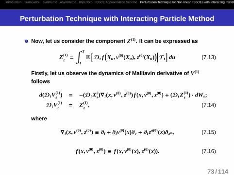
Perturbation Technique with Interacting Particle Method
([21], [14])
We will provide a straightforward simulation scheme to solve nonlinearFBSDEs at each order of perturbative approximation.
Due to the convoluted nature of the perturbative expansion, it containsmulti-dimensional time integrations of expectation values, which makestandard Monte Carlo too time consuming.To avoid nested simulations, we applied the particle representationinspired by the ideas of branching diffusion models(e.g. McKean (1975),Fujita (1966), Ikeda-Nagasawa-Watanabe (1965,1966,1968),Nagasawa-Sirao (1969)).Comparing with the direct application of the branching diffusion method,our method is expected to be less numerically intensive since theinterested system is already decomposed into a set of linear problems.
66 / 114

Introduction Framework Symmetric Asymmetric Imperfect FBSDE Approximation Scheme Perturbation Technique for Non-linear FBSDEs with Interacting Particle Method
. . . . . . . . . . . . . . . . . . . . .
Numerical Example References
Perturbation Technique with Interacting Particle Method
Again, let us introduce the perturbation parameter ϵ: dV(ϵ)s = −ϵ f (Xs,V
(ϵ)s , Z
(ϵ)s )ds+ Z(ϵ)
s · dWs
V(ϵ)T= Ψ(XT),
(7.1)
where Xt ∈ Rd is assumed to follow a generic Markovian forward SDE
dXs = γ0(Xs)ds+ γ(Xs) · dWs; Xt = xt . (7.2)
Let us fix the initial time as t. We denote the Malliavin derivative ofXu (u ≥ t) at time t as
Dt Xu ∈ Rr×d. (7.3)
67 / 114

Introduction Framework Symmetric Asymmetric Imperfect FBSDE Approximation Scheme Perturbation Technique for Non-linear FBSDEs with Interacting Particle Method
. . . . . . . . . . . . . . . . . . . . .
Numerical Example References
Perturbation Technique with Interacting Particle Method
Its dynamics in terms of the future time u is specified by stochastic flow,(Yt,u)i
j= ∂x j
tXi
u
d(Yt,u)ij= ∂kγ
i0(Xu)(Yt,u)k
jdu+ ∂kγ
ia(Xu)(Yt,u)k
jdWa
u
(Yt,t)ij= δi
j(7.4)
where ∂k denotes the differential with respect to the k-th component ofX, and δi
jdenotes Kronecker delta. Here, i and j run through 1, · · · , d
and 1, · · · , r for a. Here, we adopt Einstein notation which assumesthe summation of all the paired indexes.
Then, it is well-known that
(Dt Xiu)a = (Yt,uγ(xt))i
a,
where a ∈ 1, · · · , r is the index of r-dimensional Brownian motion.
68 / 114

Introduction Framework Symmetric Asymmetric Imperfect FBSDE Approximation Scheme Perturbation Technique for Non-linear FBSDEs with Interacting Particle Method
. . . . . . . . . . . . . . . . . . . . .
Numerical Example References
Perturbation Technique with Interacting Particle Method
ϵ-0th order: For the zeroth order, it is easy to see
V(0)t= E
[Ψ(XT)
∣∣∣∣Ft
](7.5)
Za(0)t
= E[∂iΨ(XT)(YtTγ(Xt))i
a
∣∣∣∣Ft
]. (7.6)
It is clear that they can be evaluated by standard Monte Carlosimulation. However, for their use in higher order approximation, it iscrucial to obtain explicit approximate expressions for these twoquantities. (e.g. Hagan et al.[2002], asymptotic expansion technique)
In the following, let us suppose we have obtained the solutions up to agiven order of asymptotic expansion, and write each of them as afunction of xt : V(0)
t= v(0)(xt)
Z(0)t= z(0)(xt).
(7.7)
69 / 114

Introduction Framework Symmetric Asymmetric Imperfect FBSDE Approximation Scheme Perturbation Technique for Non-linear FBSDEs with Interacting Particle Method
. . . . . . . . . . . . . . . . . . . . .
Numerical Example References
Perturbation Technique with Interacting Particle Method
ϵ-1st order:
V(1)t=
∫ T
tE[f (Xu,V
(0)u , Z
(0)u )
∣∣∣∣Ft
]du
=
∫ T
tE[f(Xu, v(0)(Xu), z(0)(Xu)
)∣∣∣∣Ft
]du (7.8)
Next, define the new process for (s > t):
V(1)ts= e
∫ st λu duV(1)
s , (7.9)
where deterministic positive process λt (It can be a positive constantfor the simplest case.).
70 / 114

Introduction Framework Symmetric Asymmetric Imperfect FBSDE Approximation Scheme Perturbation Technique for Non-linear FBSDEs with Interacting Particle Method
. . . . . . . . . . . . . . . . . . . . .
Numerical Example References
Perturbation Technique with Interacting Particle Method
Then, its dynamics is given by
dV(1)ts= λsV
(1)ts
ds− λs f ts(Xs, v(0)(Xs), z(0)(Xs))ds+ e∫ s
t λu duZ(1)s · dWs ,
where
f ts(x, v(0)(x), z(0)(x)) =1
λse∫ s
t λu du f (x, v(0)(x), z(0)(x)).
Since we have V(1)t t= V(1)
t, one can easily see the following relation
holds:
V(1)t= E
[∫ T
te−
∫ ut λsdsλu f tu(Xu, v(0)(Xu), z(0)(Xu))du
∣∣∣∣∣∣Ft
](7.10)
As in credit risk modeling (e.g. Bielecki-Rutkowski [2002]), it is thepresent value of default payment where the default intensity is λs withthe default payoff at s(> t) as f ts(Xs, v(0)(Xs), z(0)(Xs)). Thus, we obtainthe following proposition.
71 / 114

Introduction Framework Symmetric Asymmetric Imperfect FBSDE Approximation Scheme Perturbation Technique for Non-linear FBSDEs with Interacting Particle Method
. . . . . . . . . . . . . . . . . . . . .
Numerical Example References
Perturbation Technique with Interacting Particle Method
.
Proposition
.
.
.
. ..
.
.
The V(1)t
in (7.8) can be equivalently expressed as
V(1)t= 1τ>tE
[1τ<T f tτ
(Xτ, v(0)(Xτ), z(0)(Xτ)
)∣∣∣∣Ft
]. (7.11)
Here τ is the interaction time where the interaction is drawn independently from
Poisson distribution with an arbitrary deterministic positive intensity process λt . fis defined as
f ts(x, v(0)(x), z(0)(x)) =1
λse∫ s
t λu du f (x, v(0)(x), z(0)(x)) . (7.12)
72 / 114
Introduction Framework Symmetric Asymmetric Imperfect FBSDE Approximation Scheme Perturbation Technique for Non-linear FBSDEs with Interacting Particle Method
. . . . . . . . . . . . . . . . . . . . .
Numerical Example References
Perturbation Technique with Interacting Particle Method
Now, let us consider the component Z(1). It can be expressed as
Z(1)t=
∫ T
tE
[Dt f
(Xu, v(0)(Xu), z(0)(Xu)
)∣∣∣∣Ft
]du (7.13)
Firstly, let us observe the dynamics of Malliavin derivative of V(1)
follows
d(DtV(1)s ) = −(Dt Xi
s)∇i(x, v(0), z(0)) f (x, v(0), z(0)) + (Dt Z(1)s ) · dWs;
DtV(1)t= Z(1)
t, (7.14)
where
∇i(x, v(0), z(0)) ≡ ∂i + ∂iv(0)(x)∂v + ∂i za(0)(x)∂za , (7.15)
f (x, v(0), z(0)) ≡ f (x, v(0)(x), z(0)(x)). (7.16)
73 / 114

Introduction Framework Symmetric Asymmetric Imperfect FBSDE Approximation Scheme Perturbation Technique for Non-linear FBSDEs with Interacting Particle Method
. . . . . . . . . . . . . . . . . . . . .
Numerical Example References
Perturbation Technique with Interacting Particle Method
Define, for (s > t),
DtV(1)s = e
∫ st λu du(DtV
(1)s ). (7.17)
Then, its dynamics can be written as
d(DtV(1)s ) = λs(DtV
(1)s )ds− λs(Dt X i
s)∇i(Xs, v(0), z(0)) f ts(Xs, v(0), z(0))ds
+e∫ s
t λu du(Dt Z(0)s ) · dWs. (7.18)
We again have
DtV(1)t= Z(1)
t. (7.19)
Hence,
Z(1)t= E
[∫ T
te−
∫ ut λsdsλu(Dt Xi
u)∇i(Xu, v(0), z(0)) f tu(Xu, v(0), z(0))du
∣∣∣∣∣∣Ft
].(7.20)
74 / 114

Introduction Framework Symmetric Asymmetric Imperfect FBSDE Approximation Scheme Perturbation Technique for Non-linear FBSDEs with Interacting Particle Method
. . . . . . . . . . . . . . . . . . . . .
Numerical Example References
Perturbation Technique with Interacting Particle Method
Thus, following the same argument for the previous proposition, wehave the result below:
.
Proposition
.
.
.
. ..
.
.
Z(1)t
in (7.13) is equivalently expressed as
Za(1)t= 1τ>tE
[1τ<T(Ytτγ(Xτ))i
a∇i(Xτ, v(0), z(0)) f tτ(Xτ, v(0), z(0))∣∣∣∣Ft
](7.21)
where the definitions of random time τ and the positive deterministic process λ
are the same as those in the previous proposition.
75 / 114

Introduction Framework Symmetric Asymmetric Imperfect FBSDE Approximation Scheme Perturbation Technique for Non-linear FBSDEs with Interacting Particle Method
. . . . . . . . . . . . . . . . . . . . .
Numerical Example References
Perturbation Technique with Interacting Particle MethodMonte Carlo Method
Now, we have a new particle interpretation of (V(1), Z(1)) as follows:
V(1)t= 1τ>tE
[1τ<T f tτ
(Xτ, v(0), z(0)
)∣∣∣∣Ft
](7.22)
Z(1)t= 1τ>tE
[1τ<T(Yt,τγ(Xτ))i∇i(Xτ, v(0), z(0)) f tτ(Xτ, v(0), z(0))
∣∣∣∣Ft
](7.23)
which allows efficient time integration with the following Monte Carloscheme:• Run the diffusion processes of X and Y• Carry out Poisson draw with probability λs∆s at each time s and if ”one” isdrawn, set that time as τ.• Then stores the relevant quantities at τ, or in the case of (τ > T) stores 0.• Repeat the above procedures and take their expectation.
76 / 114

Introduction Framework Symmetric Asymmetric Imperfect FBSDE Approximation Scheme Perturbation Technique for Non-linear FBSDEs with Interacting Particle Method
. . . . . . . . . . . . . . . . . . . . .
Numerical Example References
Z(2)t
The second order stochastic flow: for t < s < u,
(Γt,s,u)ijk
:=∂2
∂x jt∂xk
s
Xiu;
((Γt,s,s)i
jk= 0
).
77 / 114

Introduction Framework Symmetric Asymmetric Imperfect FBSDE Approximation Scheme Perturbation Technique for Non-linear FBSDEs with Interacting Particle Method
. . . . . . . . . . . . . . . . . . . . .
Numerical Example References
Figure:
78 / 114

Introduction Framework Symmetric Asymmetric Imperfect FBSDE Approximation Scheme Perturbation Technique for Non-linear FBSDEs with Interacting Particle Method
. . . . . . . . . . . . . . . . . . . . .
Numerical Example References
Numerical Example
An example for pre-default values with imperfect collateralization 14:
The counter party sells OTC European options on WTI futures. 15
For simplicity, we consider a unilateral case, where counter party isdefaultable, while the investor is default-free, and the collateral isposted as the same currency as the payment currency (that is, thecurrency is USD).
We consider the following imperfect collateral cases:
No collateralCash collateral with time-lagAsset collateral with time-lag
14As for an application to American option pricing, please see [11]15Later, we will see a basket option on WTI and Brent futures.
79 / 114

Introduction Framework Symmetric Asymmetric Imperfect FBSDE Approximation Scheme Perturbation Technique for Non-linear FBSDEs with Interacting Particle Method
. . . . . . . . . . . . . . . . . . . . .
Numerical Example References
Model
CIR model for the hazard rate process ( h).
SABR model for WTI futures price process ( S and ν).
Log-Normal model for a collateral asset price process ( A).
dht = κ (θ − ht) dt + γ√
ht c1dW1t ; h0 = h0 (8.1)
dSt = µiSt dt + νt (St)β (
2∑η=1
c2,ηdWηt); S0 = s0, (8.2)
dνt = σννt(3∑η=1
c3,ηdWηt); ν0 = ν0, (8.3)
dAt = µA At dt + σA At(4∑η=1
c4,ηdWηt); A0 = a0. (8.4)
80 / 114

Introduction Framework Symmetric Asymmetric Imperfect FBSDE Approximation Scheme Perturbation Technique for Non-linear FBSDEs with Interacting Particle Method
. . . . . . . . . . . . . . . . . . . . .
Numerical Example References
Model
The dynamics of pre-default value V can be described by a non-linearFBSDE: dVt = rV t dt − f (ht ,Vt , Γt)dt + Z t · dWt
VT = (ST − K)+ or (K − ST)+ ,(8.5)
where
Γt : collateral process(e.g. cash collateral with a constant time lag ∆ : Γt = Vt−∆)
r(risk free rate), c(collateral rate), l(loss rate) : nonnegative constantsfor simplicity. 16
We put ϵ in front of the driver, f to apply our perturbation technique withinteracting particle method.
16[14] Later, we will see a more general case, where a stochastic collateral cost is takeninto account.
81 / 114

Introduction Framework Symmetric Asymmetric Imperfect FBSDE Approximation Scheme Perturbation Technique for Non-linear FBSDEs with Interacting Particle Method
. . . . . . . . . . . . . . . . . . . . .
Numerical Example References
Model
Counter party does not post collateral or posts collateral with theconstant time-lag ( ∆) by cash or an asset A.
no collateral case:
f (ht ,Vt , Γt) = −lh t(Vt)+. (8.6)
time-lag collateral case
cash collateral:
f (ht ,Vt , Γt) = (r − c)Vt−∆
−lh t (Vt − Vt−∆)+ , (8.7)
asset collateral:
f (ht ,Vt , Γt) = (r − c)Vt−∆
(At
At−∆
)−lh t
(Vt − Vt−∆
(At
At−∆
))+. (8.8)
82 / 114

Introduction Framework Symmetric Asymmetric Imperfect FBSDE Approximation Scheme Perturbation Technique for Non-linear FBSDEs with Interacting Particle Method
. . . . . . . . . . . . . . . . . . . . .
Numerical Example References
Parameters
We use the data of CME WTI option and futures prices.The maturity of the underlying futures is DEC 15, and the maturity of WTI optionis Nov 17, 2015.
Parameters of WTI futures are obtained by calibration to the market values offutures option prices on July 10, 2012.
We assume that the risk free rate r is equal to collateral rate c.
The discount rate is c = 0.295% which is calculated by OIS with the samematurity as the option maturity.
The recovery rate is R = 0 (i.e. l = 1).
Calibrated parameters are as follows 17:
Table: Parameters of WTI DEC15 in SABR model
S(0) β ν(0) σν ρ
WTI DEC15 84.48 0.5 2.117 0.410 -0.112
17As futures options traded in CME(WTI) are American type, we calibrate to Europeanoption prices with the implied BS(log-normal) volatilities that are obtained by a binomialmethod.
83 / 114

Introduction Framework Symmetric Asymmetric Imperfect FBSDE Approximation Scheme Perturbation Technique for Non-linear FBSDEs with Interacting Particle Method
. . . . . . . . . . . . . . . . . . . . .
Numerical Example References
Parameters, Monte Carlo
We use the results of Denault et al., 2009 [ 7] for the parameters ofhazard rate processes.
We calculate the pre-default value of European option whose maturityis the same as that of futures option.
The details of Monte Carlo method simulation are as follows:
time step size is 1/200 years.the number of trial is 10 million.Hagan et al. formula [2002] is used for evaluation of default-freeEuropean options, that is V(0).
84 / 114

Introduction Framework Symmetric Asymmetric Imperfect FBSDE Approximation Scheme Perturbation Technique for Non-linear FBSDEs with Interacting Particle Method
. . . . . . . . . . . . . . . . . . . . .
Numerical Example References
Analysis
We check the following points.
correlation effect: ( S, h), (S, v), (h, v), (S, A), (ν, A) and ( h, A).collateral effect: no collateral, cash collateral with constanttime-lag or asset collateral with constant time-lag.rating effect: from Aaa to B.the second order value’s effect.maturity effect: from 2 years to 10 years.
85 / 114

Introduction Framework Symmetric Asymmetric Imperfect FBSDE Approximation Scheme Perturbation Technique for Non-linear FBSDEs with Interacting Particle Method
. . . . . . . . . . . . . . . . . . . . .
Numerical Example References
Correlation Effect
Firstly, we test the correlation effects among the hazard rates, theunderlying asset price, its volatility and the collateral asset price.In this example, we set the following assumptions.
the correlations which are not explicitly specified are set to be 0.
parameters of the hazard rate processes are those of Baa rating.
parameters of the collateral asset are µA = 0 and σA = 50%.
the time-lag ( ∆) of collateral is 0.1.
strike price is ATM.
86 / 114

Introduction Framework Symmetric Asymmetric Imperfect FBSDE Approximation Scheme Perturbation Technique for Non-linear FBSDEs with Interacting Particle Method
. . . . . . . . . . . . . . . . . . . . .
Numerical Example References
Correlation Effect - No Collateral
Table: Pre-default values of call option contracts without collateral
Correlation -0.7 -0.35 0 0.35 0.7
S and h 0th 14.648 14.648 14.648 14.648 14.6481st -0.784 -0.987 -1.220 -1.465 -1.7422nd 0.027 0.043 0.065 0.091 0.123Total 13.890 13.704 13.492 13.273 13.029
S and ν 0th 13.789 14.338 14.648 14.719 14.5531st -1.147 -1.192 -1.220 -1.231 -1.2222nd 0.061 0.063 0.065 0.066 0.065Total 12.703 13.210 13.492 13.554 13.397
h and ν 0th 14.648 14.648 14.648 14.648 14.6481st -1.055 -1.134 -1.220 -1.312 -1.4102nd 0.050 0.057 0.065 0.074 0.085Total 13.642 13.570 13.492 13.410 13.322
When the correlation between S and h increases ( −0.7 → +0.7), the absolutevalues of the first and the second order become larger. (High correlationbetween S and h means that the default risk becomes high when the optionvalue is high.)
87 / 114

Introduction Framework Symmetric Asymmetric Imperfect FBSDE Approximation Scheme Perturbation Technique for Non-linear FBSDEs with Interacting Particle Method
. . . . . . . . . . . . . . . . . . . . .
Numerical Example References
Correlation Effect - Cash Collateral
Table: Pre-default values of call option contracts with cash collateral
Correlation -0.7 -0.35 0 0.35 0.7
S and h 0th 14.648 14.648 14.648 14.648 14.6481st -0.116 -0.137 -0.160 -0.185 -0.2112nd 0.00004 0.00004 0.00004 0.00004 0.00004Total 14.532 14.511 14.488 14.463 14.436
S and ν 0th 13.789 14.338 14.648 14.719 14.5531st -0.127 -0.144 -0.160 -0.174 -0.1872nd 0.00004 0.00004 0.00004 0.00004 0.00004Total 13.663 14.194 14.488 14.545 14.366
h and ν 0th 14.648 14.648 14.648 14.648 14.6481st -0.130 -0.144 -0.160 -0.177 -0.1952nd 0.00004 0.00004 0.00004 0.00004 0.00004Total 14.518 14.503 14.488 14.471 14.452
The effect of the second order value seems negligible under collateralizationwith this level of time-lag.
88 / 114

Introduction Framework Symmetric Asymmetric Imperfect FBSDE Approximation Scheme Perturbation Technique for Non-linear FBSDEs with Interacting Particle Method
. . . . . . . . . . . . . . . . . . . . .
Numerical Example References
Correlation Effect - Asset Collatral
Table: Pre-default values of call option contracts with asset collateral
Correlation -0.7 -0.35 0 0.35 0.7
S and h 0th 14.648 14.648 14.648 14.648 14.6481st -0.128 -0.154 -0.183 -0.214 -0.2492nd 0.0001 0.0002 0.0003 0.0004 0.0006Total 14.520 14.494 14.465 14.433 14.399
S and ν 0th 13.789 14.338 14.648 14.719 14.5531st -0.154 -0.169 -0.183 -0.194 -0.2042nd 0.0003 0.0003 0.0003 0.0003 0.0003Total 13.635 14.169 14.465 14.525 14.350
h and ν 0th 14.648 14.648 14.648 14.648 14.6481st -0.152 -0.166 -0.183 -0.201 -0.2202nd 0.0002 0.0003 0.0003 0.0003 0.0004Total 14.496 14.481 14.465 14.447 14.428
The first order value with asset collateral is about 1.2 times as large as that withcash collateral.
The effect of the second order value also seems negligible.
89 / 114

Introduction Framework Symmetric Asymmetric Imperfect FBSDE Approximation Scheme Perturbation Technique for Non-linear FBSDEs with Interacting Particle Method
. . . . . . . . . . . . . . . . . . . . .
Numerical Example References
Correlation Effect - Asset Collateral
Table: Pre-default values of call option contracts with asset collateral
Correlation -0.7 -0.35 0 0.35 0.7
S and A 0th 14.648 14.648 14.648 14.648 14.6481st -0.220 -0.202 -0.183 -0.160 -0.1322nd 0.0007 0.0005 0.0003 0.0001 0.0000Total 14.428 14.446 14.465 14.487 14.515
ν and A 0th 14.648 14.648 14.648 14.648 14.6481st -0.192 -0.188 -0.183 -0.178 -0.1722nd 0.0004 0.0004 0.0003 0.0002 0.0002Total 14.455 14.460 14.465 14.470 14.475
h and A 0th 14.648 14.648 14.648 14.648 14.6481st -0.192 -0.188 -0.183 -0.178 -0.1742nd 0.0004 0.0004 0.0003 0.0002 0.0002Total 14.456 14.460 14.465 14.470 14.474
Correlation effect between the underlying asset price and the collateral assetprice seems similar order as the one between the underlying asset price andthe hazard rate.
When the correlation between S and A is negative, the increase in the optionpremium and the decrease in the collateral value occur simultaneously. (Thatis, it requires more collateral.) 90 / 114

Introduction Framework Symmetric Asymmetric Imperfect FBSDE Approximation Scheme Perturbation Technique for Non-linear FBSDEs with Interacting Particle Method
. . . . . . . . . . . . . . . . . . . . .
Numerical Example References
Rating Effect - No Collateral
Table: Pre-default values of call option contracts without collateral
Strike 70 80 85 90 100
Aaa 0th 22.658 16.798 14.333 12.179 8.7441st -0.474 -0.351 -0.300 -0.254 -0.1822nd 0.005 0.004 0.003 0.003 0.002Total 22.189 16.450 14.036 11.928 8.564
Baa 0th 22.658 16.798 14.333 12.179 8.7441st -1.879 -1.392 -1.186 -1.007 -0.7202nd 0.100 0.074 0.063 0.054 0.038Total 20.879 15.480 13.210 11.226 8.062
B 0th 22.658 16.798 14.333 12.179 8.7441st -7.877 -5.833 -4.972 -4.219 -3.0172nd 2.155 1.595 1.359 1.153 0.823Total 16.936 12.560 10.720 9.113 6.551
the worse is the rating, the more important the second order becomes.
For the case of single B, if the second order value is not taken into account, thepre-default value is more than 10% different from the first order pre-defaultvalue.
91 / 114

Introduction Framework Symmetric Asymmetric Imperfect FBSDE Approximation Scheme Perturbation Technique for Non-linear FBSDEs with Interacting Particle Method
. . . . . . . . . . . . . . . . . . . . .
Numerical Example References
Rating Effect - Asset Collateral
Table: Pre-default values of call option contracts with asset collateral
Strike 70 80 85 90 100
Aaa 0th 22.658 16.798 14.333 12.179 8.7441st -0.064 -0.051 -0.045 -0.040 -0.0312nd 0.00003 0.00002 0.00002 0.00001 0.00001Total 22.594 16.747 14.288 12.139 8.714
Baa 0th 22.658 16.798 14.333 12.179 8.7441st -0.250 -0.199 -0.177 -0.156 -0.1202nd 0.00047 0.00035 0.00030 0.00025 0.00018Total 22.409 16.599 14.157 12.024 8.624
B 0th 22.658 16.798 14.333 12.179 8.7441st -1.029 -0.822 -0.729 -0.644 -0.4972nd 0.00996 0.00737 0.00628 0.00533 0.00380Total 21.639 15.983 13.610 11.541 8.251
The effect of the second order value seems negligible under collateralizationwith this level of time lag, even if the rating is single B.
92 / 114

Introduction Framework Symmetric Asymmetric Imperfect FBSDE Approximation Scheme Perturbation Technique for Non-linear FBSDEs with Interacting Particle Method
. . . . . . . . . . . . . . . . . . . . .
Numerical Example References
Rating Effect - Implied Volatility (No Collateral)
Figure: Implied volatilities of call options without collateral
13%
15%
17%
19%
21%
23%
25%
27%
70 80 85 90 100
Default Free Aaa Aa A Baa Ba B
The shape of the skew of rating B is different from that of rating Aaa. Thedifference of IV from the default-free case is larger for ITM, and the size ofdifference varies in rating.
93 / 114

Introduction Framework Symmetric Asymmetric Imperfect FBSDE Approximation Scheme Perturbation Technique for Non-linear FBSDEs with Interacting Particle Method
. . . . . . . . . . . . . . . . . . . . .
Numerical Example References
Rating Effect - Implied Volatility (Asset Collateral)
Figure: Implied volatilities of European call options with risky asset collateral
21%
22%
23%
24%
25%
26%
27%
70 80 85 90 100
Default Free Aaa Aa A Baa Ba B
In this case, the shape of all ratings is similar.
The level of implied volatility is different in rating.
94 / 114

Introduction Framework Symmetric Asymmetric Imperfect FBSDE Approximation Scheme Perturbation Technique for Non-linear FBSDEs with Interacting Particle Method
. . . . . . . . . . . . . . . . . . . . .
Numerical Example References
Correlation Effect ( S, h) - Implied Volatility (Rating : B)
Figure: Implied volatilities of European call and put options without collateral
8%10%12%14%16%18%20%22%24%26%28%
70 80 85 90 100
Default Free Call ρS,h = 0.7 Call ρS,h = 0
Call ρS,h = -0.7 Put ρS,h = 0.7 Put ρS,h = 0
Put ρS,h = -0.7
When the correlation between the underlying asset price and the hazard ratebecomes high, a call option’s implied volatility becomes low.
This is because a default probability will increase if the price rises (that is, theoption value rises).
For the case of put options, the shape is reversed.95 / 114

Introduction Framework Symmetric Asymmetric Imperfect FBSDE Approximation Scheme Perturbation Technique for Non-linear FBSDEs with Interacting Particle Method
. . . . . . . . . . . . . . . . . . . . .
Numerical Example References
The Second Order Effect - Implied Volatility (Baa)
Figure: Implied volatilities of European call and put options without collateral
19%
20%
21%
22%
23%
24%
25%
26%
27%
70 80 85 90 100
Default Free Baa 1st Call Baa 2nd Call
Baa 1st Put Baa 2nd Put
The difference between the first and the second is not so large in this case.
96 / 114

Introduction Framework Symmetric Asymmetric Imperfect FBSDE Approximation Scheme Perturbation Technique for Non-linear FBSDEs with Interacting Particle Method
. . . . . . . . . . . . . . . . . . . . .
Numerical Example References
The Second Order Effect - Implied Volatility (B)
Figure: Implied volatilities of European call and put options without collateral
5%
7%
9%
11%
13%
15%
17%
19%
21%
23%
25%
27%
70 80 85 90 100
Default Free B 1st Call B 2nd Call B 1st Put B 2nd Put
It seems better to take the second order value into account.
97 / 114

Introduction Framework Symmetric Asymmetric Imperfect FBSDE Approximation Scheme Perturbation Technique for Non-linear FBSDEs with Interacting Particle Method
. . . . . . . . . . . . . . . . . . . . .
Numerical Example References
Maturity Effect - No Collateral (Baa)
Next graph shows the values of 0th (default free), 1st and 2nd order price of the ATMoption without collateral in Baa rating.
Figure: Pre-default values of call option contracts without collateral
10
13
16
19
22
25
28
2Y 4Y 6Y 8Y 10Y
0th 0th + 1st 0th + 1st + 2nd
For the long maturity case, the second order value has larger impact on thepre-default value.
For the case of 10 years maturity, the 2nd order affects by more than 5%.98 / 114

Introduction Framework Symmetric Asymmetric Imperfect FBSDE Approximation Scheme Perturbation Technique for Non-linear FBSDEs with Interacting Particle Method
. . . . . . . . . . . . . . . . . . . . .
Numerical Example References
Maturity Effect - Asset Collateral (Baa)
Figure: Pre-default values of call option contracts with asset collateral
10
13
16
19
22
25
28
2Y 4Y 6Y 8Y 10Y
0th 0th + 1st 0th + 1st + 2nd
When we post the collateral, the second order effect does not increase.
The second order effect can be ignored even if the maturity is more than 10years.
99 / 114

Introduction Framework Symmetric Asymmetric Imperfect FBSDE Approximation Scheme Perturbation Technique for Non-linear FBSDEs with Interacting Particle Method
. . . . . . . . . . . . . . . . . . . . .
Numerical Example References
Stochastic Collateral Cost
Next, we consider a more general case:
dVt = cVt dt − f (yt , yt , ht ,Vt , Γt)dt + Z · dWt , (8.9)
where
f (yt , yt , ht ,Vt , Γt) = ytΓt − ytVt − lh t (Vt − Γt)+ (8.10)
yt = r t − c(collateral cost of USD ) (8.11)
yt = r t − ct(collateral cost of Γt) (8.12)
For numerical examples, we set y ≡ 0 and suppose yt = r t − c where rfollows a CIR process with a nonnegative constant c. Then, we put ϵ infront of f to apply our perturbation technique with interacting particlemethod.
100 / 114

Introduction Framework Symmetric Asymmetric Imperfect FBSDE Approximation Scheme Perturbation Technique for Non-linear FBSDEs with Interacting Particle Method
. . . . . . . . . . . . . . . . . . . . .
Numerical Example References
Stochastic Collateral Cost
CIR model for risk free rate process ( r).
drt = κr (θr − r t) dt + γr√
r t(5∑η=1
c5,ηdWηt); r0 = r(0). (8.13)
Table: Parameters of USD risk free rate process
r(0) κr θr γr
USD Risk Free Rate 1% 0.2 1% 0.05
The other parameters are the same as before.
The rating of counter party is Baa.
We check the following points.
correlation effect: ( S, h), (S, y), and ( h, y).collateral effect: no collateral, cash collateral with constanttime-lag 0.1.
101 / 114

Introduction Framework Symmetric Asymmetric Imperfect FBSDE Approximation Scheme Perturbation Technique for Non-linear FBSDEs with Interacting Particle Method
. . . . . . . . . . . . . . . . . . . . .
Numerical Example References
Correlation Effect - No Collateral
Table: Correlation Effects - No Collateral
Correlation -0.7 -0.35 0 0.35 0.7
S and h 0th 14.648 14.648 14.648 14.648 14.6481st -1.129 -1.335 -1.565 -1.821 -2.1002nd 0.051 0.072 0.099 0.131 0.170Total 13.570 13.385 13.181 12.958 12.717
S and y 0th 14.648 14.648 14.648 14.648 14.6481st -1.418 -1.488 -1.565 -1.650 -1.7422nd 0.083 0.090 0.099 0.109 0.119Total 13.313 13.250 13.181 13.106 13.025
h and y 0th 14.648 14.648 14.648 14.648 14.6481st -1.565 -1.565 -1.565 -1.565 -1.5652nd 0.093 0.096 0.099 0.102 0.105Total 13.176 13.179 13.181 13.184 13.187
Change in the correlation between S and y affects on the value by at most 2 %, while
change in the correlation between S and h does by around 6%.
102 / 114
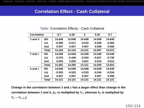
Introduction Framework Symmetric Asymmetric Imperfect FBSDE Approximation Scheme Perturbation Technique for Non-linear FBSDEs with Interacting Particle Method
. . . . . . . . . . . . . . . . . . . . .
Numerical Example References
Correlation Effect - Cash Collateral
Table: Correlation Effects - Cash Collateral
Correlation -0.7 -0.35 0 0.35 0.7
S and h 0th 14.648 14.648 14.648 14.648 14.6481st -0.490 -0.511 -0.533 -0.558 -0.5842nd 0.007 0.007 0.007 0.008 0.008Total 14.164 14.144 14.121 14.097 14.072
S and y 0th 14.648 14.648 14.648 14.648 14.6481st -0.370 -0.448 -0.533 -0.627 -0.7302nd 0.003 0.005 0.007 0.010 0.014Total 14.281 14.205 14.121 14.030 13.931
h and y 0th 14.648 14.648 14.648 14.648 14.6481st -0.533 -0.533 -0.533 -0.534 -0.5342nd 0.007 0.007 0.007 0.007 0.008Total 14.121 14.121 14.121 14.121 14.121
Change in the correlation between S and y has a larger effect than change in the
correlation between S and h, (yt is multiplied by Vt , whereas ht is multiplied by
Vt − Vt−∆.)
103 / 114

Introduction Framework Symmetric Asymmetric Imperfect FBSDE Approximation Scheme Perturbation Technique for Non-linear FBSDEs with Interacting Particle Method
. . . . . . . . . . . . . . . . . . . . .
Numerical Example References
Basket Option
Next, we consider about a basket option of WTI and Brent.
To calculate V(0) analytically, we use the asymptotic expansion method (pleasesee [39] for the detail).
The maturity of the underlying futures is DEC 15.
The maturity of basket option is Nov 10, 2015.
The discount rate is c = 0.295% which is calculated by OIS with the samematurity as the option maturity.
The parameters of the underlying asset prices are obtained by calibration to themarket values of futures options on July 10, 2012.
Calibrated parameters are follows. 18 :
Table: Parameters of Brent DEC15 in SABR model
S(0) β ν(0) σν ρ
Brent DEC15 90.14 0.5 2.184 0.446 -0.044
18As futures options traded in ICE(Brent) are American type, we calibrate to Europeanoption prices with the implied BS(log-normal) volatilities that are obtained by a binomialmethod.
104 / 114

Introduction Framework Symmetric Asymmetric Imperfect FBSDE Approximation Scheme Perturbation Technique for Non-linear FBSDEs with Interacting Particle Method
. . . . . . . . . . . . . . . . . . . . .
Numerical Example References
Basket Option
The correlation between WTI futures price (or Brent futures price) andBrent volatility (or WTI volatility) is set as the same value as thecorrelation between WTI futures price (or Brent futures Price) and WTIvolatility (or Brent volatility).
The correlations between WTI futures price (or volatility) and Brentfutures price (or volatility) are calculated by using logarithmichistorical price changes for the 30 days before July 10, 2012.
The correlation between WTI future price and Brent future price is0.980, and the correlation between WTI volatility and Brent volatility is0.907.
105 / 114

Introduction Framework Symmetric Asymmetric Imperfect FBSDE Approximation Scheme Perturbation Technique for Non-linear FBSDEs with Interacting Particle Method
. . . . . . . . . . . . . . . . . . . . .
Numerical Example References
Basket Option
Table: Pre-default values of call option contracts without collateral
Strike 140 160 170 180 200
Aaa 0th 49.798 37.475 32.224 27.590 20.0831st -1.036 -0.780 -0.671 -0.575 -0.4182nd 0.011 0.009 0.007 0.006 0.005Total 48.774 36.704 31.561 27.021 19.669
Baa 0th 49.798 37.475 32.224 27.590 20.0831st -4.101 -3.089 -2.657 -2.276 -1.6582nd 0.217 0.164 0.141 0.121 0.088Total 45.915 34.550 29.708 25.435 18.513
B 0th 49.798 37.475 32.224 27.590 20.0831st -17.176 -12.937 -11.130 -9.534 -6.9462nd 4.680 3.531 3.041 2.607 1.904Total 37.303 28.069 24.135 20.662 15.041
Moreover, applying the asymptotic expansion method, we are able tocalculate pre-default values of various type of basket options. (Pleasesee [39] for the detail.)
106 / 114

Introduction Framework Symmetric Asymmetric Imperfect FBSDE Approximation Scheme Perturbation Technique for Non-linear FBSDEs with Interacting Particle Method
. . . . . . . . . . . . . . . . . . . . .
Numerical Example References
References I
[1] Bianchetti, M. (2012), ”Two curves, one price, ”online paper in Risk.net.
[2] Bielecki., Rutkowski (2000), Credit Risk: Modeling,Valuation and Hedging ,Springer.
[3] Brigo, D., Capponi, A. (2009), ”Bilateral counterparty risk valuation withstochastic dynamical models and application to Credit Default Swaps”.
[4] Carmona (editor) (2009). ”Indifference Pricing,” Princeton University Press.
[5] Collin-Dufresne, P., Goldstein, R., and Hugonnier, J., ”A General Formula forValuing Defaultable Securities,” Econometrica (2004), 72, 1377-1407.
[6] Crepey, S., (2012a,b), ”Bilateral Counterparty Risk under Funding Constraints -Part I:Pricing, Part II:CVA ”, Forthcoming in Mathematical Finance.
[7] Denalut, M., Gauthier, G. and Simonato, J-G., ”ESTIMATION OF PHYSICALINTENSITY MODELS FOR DEFAULT RISK,” The Journal of Futures Markets, Vol.29, No. 2, 95-113 (2009).
[8] Duffie, D., Huang, M., ”Swap Rates and Credit Quality,” Journal of Finance (1996)Vol. 51, No. 3, 921.
107 / 114

Introduction Framework Symmetric Asymmetric Imperfect FBSDE Approximation Scheme Perturbation Technique for Non-linear FBSDEs with Interacting Particle Method
. . . . . . . . . . . . . . . . . . . . .
Numerical Example References
References II
[9] P.S.Hagan, D.Kumar, A.S.Lesniewski and D.E.Woodward, Managing smile risk ,Willmott Magazine, 2002, 84-108.
[10] El Karoui, N., Peng, S.G., and Quenez, M.C. (1997). ”Backward stochasticdifferential equations in finance,” Math. Finance 7 1-71.
[11] Fujii, M., Sato, S., Takahashi, A.,2012, ”A BSDE Approach and a new MonteCarlo scheme for American-style Options”, Preprint.
[12] Fujii, M., Shimada, Y., Takahashi, A., ”A note on construction of multiple swapcurves with and without collateral,” FSA Research Review (2010)
[13] Fujii, M., Shimada, Y., Takahashi, A., ”A Market Model of Interest Rates withDynamic Basis Spreads in the presence of Collateral and Multiple Currencies”,Wilmott Magazine (2011).
[14] Fujii, M., Shiraya, K., Takahashi, A., 2012, ”On the Computation of DerivativfesPricing under Imperfect Collateralization and CVA,” in preparation.
[15] Fujii, M., Takahashi, A., ”Modeling of Interest Rate Term Structures underCollateralization and its Implications”, KIER-TMU International Workshop onFinancial Engineering, 2010 (2011).
108 / 114

Introduction Framework Symmetric Asymmetric Imperfect FBSDE Approximation Scheme Perturbation Technique for Non-linear FBSDEs with Interacting Particle Method
. . . . . . . . . . . . . . . . . . . . .
Numerical Example References
References III
[16] Fujii, M., Takahashi, A., ”Choice of Collateral Currency”,January 2011, RiskMagazine, 120-125.
[17] Fujii, M., Takahashi, A., 2010, ”Derivative pricing under Asymmetric andImperfect Collateralization and CVA,” CARF Working paper series F-240,forthcoming in Quantitative Finance.
[18] Fujii, M., Takahashi, A., 2011, ”Collateralized CDS and Default Dependence-Implications for the Central Clearing-,” Journal of Credit Risk, Vol.8-3, Fall,2012, 97-113.
[19] Fujii, M., and Takahashi, A. (2011). ”Analytical Approximation for non-linearFBSDEs with Perturbation Scheme,” International Journal of Theoretical andApplied Finance, Vol.15-5, 2012.
[20] Fujii, M., and Takahashi, A. (2012), ”Perturbative Expansion of FBSDE in anIncomplete Market with Stochastic Volatility,” Quarterly Journal of Finance,Vol.2-3, 2012, 1250015.
109 / 114

Introduction Framework Symmetric Asymmetric Imperfect FBSDE Approximation Scheme Perturbation Technique for Non-linear FBSDEs with Interacting Particle Method
. . . . . . . . . . . . . . . . . . . . .
Numerical Example References
References IV
[21] Fujii, M,, Takahashi, A., Perturbative Expansion Technique for Non-linearFBSDEs with Interacting Particle Method , Working paper, CARF-F-278, theUniversity of Tokyo, 2012.
[22] Fujii, M., Takahashi, A., (2012), ”Interest Rate Modeling under the FullCollateralization,” as a contributing chapter in a RISK BOOK ”Interest RateModeling After The Financial Crisis”
[23] Fujita, H., ”On the blowing up of solutions of the Cauchy problem forut = ∆u + u1+α,” J. Fac. Sci. Univ. Tokyo 13 (1966), 109-124
[24] Gobet,E., LemorJ.-P. , and Warin,X. A regression-based Monte Carlo method tosolve backward stochastic differential equations , 2005.
[25] Ikeda, N., Nagasawa, M., and Watanabe, S. (1965), ”Branching Markovprocesses,” Abstracts Proc. Japan Acad. 41, 816-821.
[26] Ikeda, N., Nagasawa, M., and Watanabe, S. (1966), ”Branching Markovprocesses,” Abstracts Proc. Japan Acad. 42, 252-257, 370-375, 380-384, 719-724,1016-1021, 1022-1026.
110 / 114

Introduction Framework Symmetric Asymmetric Imperfect FBSDE Approximation Scheme Perturbation Technique for Non-linear FBSDEs with Interacting Particle Method
. . . . . . . . . . . . . . . . . . . . .
Numerical Example References
References V
[27] Ikeda, N., Nagasawa, M., and Watanabe, S., (1968), ”Branching Markovprocesses I(II),” J. Math. Kyoto Univ. 8, 233-278, 365-410.
[28] ISDA Margin Survey 2011,
[29] Kunitomo, N. and Takahashi, A. (2001), “ The Asymptotic Expansion Approachto the Valuation of Interest Rate Contingent Claims, ”Mathematical Finance,Vol. 11, 117-151.
[30] Kunitomo, N. and Takahashi, A. (2003). ”On Validity of the AsymptoticExpansion Approach in Contingent Claim Analysis,” Annals of AppliedProbability, 13, No.3, 914-952.
[31] Ma, J., and Yong, J. (2000), ”Forward-Backward Stochastic DifferentialEquations and their Applications,” Springer.
[32] Mercurio,F. (2009), ”Interest rate and the credit crunch: New formulas andmarket models, ”2009, Bloomberg Portfolio Research Paper.
[33] Morini, M. (2009), ”Solving the Puzzle in the interest Rate Market, ”available athttp://ssrn.com/abstract=1506046.
111 / 114

Introduction Framework Symmetric Asymmetric Imperfect FBSDE Approximation Scheme Perturbation Technique for Non-linear FBSDEs with Interacting Particle Method
. . . . . . . . . . . . . . . . . . . . .
Numerical Example References
References VI
[34] Nagasawa, M., Sirao, T., (1969), ”Probabilistic Treatment of the Blowing up ofSolutions for a Nonlinear Integral Equation,” Trans. Amer. Math. Soc. Vol 139,301-310.
[35] McKean, H., P., ”Application of Brownian Motion to the Equation ofKolmogorov-Petrovskii-Piskunov,” Communications on Pure and AppliedMathematics, Vol. XXVIII, 323-331 (1975).
[36] Piterbarg, V., ”Funding beyond discounting : collateral agreements andderivatives pricing” Risk Magazine (2010).
[37] Schonbucher, P., 2000 ”A Libor Market Model with Default Risk,” Working Paper,University of Bonn.
[38] Shiraya, K. and Takahashi, (2011), Pricing Average Options on Commodities ,”Journal of Futures Markets”, 31, Issue 5, 407-439.
[39] Shiraya, K. and Takahashi, (2012), Pricing Multi-Asset Cross Currency Options ,forthcoming in Journal of Futures Markets.
112 / 114

Introduction Framework Symmetric Asymmetric Imperfect FBSDE Approximation Scheme Perturbation Technique for Non-linear FBSDEs with Interacting Particle Method
. . . . . . . . . . . . . . . . . . . . .
Numerical Example References
References VII
[40] Shiraya, K,, Takahashi, A., Yamazaki, A., Pricing Swaptions under the LIBORMarket Model of Interest Rates with Local-Stochastic Volatility Models , Wilmottvolume 2012, issue 61, pp.48-63, September 2012.
[41] Takahashi, A. (1999). ”An Asymptotic Expansion Approach to PricingContingent Claims,” Asia-Pacific Financial Markets, 6, 115-151.
[42] Takahashi, A., Takehara, K., and Toda, M. (2011). ”A General ComputationScheme for a High-Order Asymptotic Expansion Method,” International Journalof Theoretical and Applied Finance, Vol.15-6, 2012.
[43] Takahashi, A., Yamada, T., An Asymptotic Expansion with Push-Down ofMalliavin Weights , SIAM Journal on Financial Mathematics Volume 3, pp 95-136,2012.
[44] Takahashi, A., Yamada, T. (2012), “An Asymptotic Expansion forForward-Backward SDEs: A Malliavin Calculus Approach,” Preprint,CARF-F-296, University of Tokyo.
113 / 114

Introduction Framework Symmetric Asymmetric Imperfect FBSDE Approximation Scheme Perturbation Technique for Non-linear FBSDEs with Interacting Particle Method
. . . . . . . . . . . . . . . . . . . . .
Numerical Example References
References VIII
[45] Takahashi, A. and Yoshida, N. (2004). “An Asymptotic Expansion Scheme forOptimal Investment Problems,” Statistical Inference for Stochastic Processes, 7,No.2, 153-188.
[46] Zariphopoulou, T., 2001, ”A Solution Approach to Valuation with UnhedgeableRisks,” Finance and Stochastics.
114 / 114