preliminary simulations of internal waves and mixing ... · preliminary simulations of internal...

ARTICLE IN PRESS

0967-0645/$ - se

doi:10.1016/j.ds

�Correspondisphere and Oc

GFDL, 201 F

States. Tel.: +1

E-mail addre

Deep-Sea Research II 53 (2006) 140–156

www.elsevier.com/locate/dsr2

Preliminary simulations of internal waves andmixing generated by finite amplitude tidal flow over

isolated topography

Sonya Legga,b,�, Karin M.H. Huijtsc

aDepartment of Physical Oceanography, Woods Hole Oceanographic Institution, Woods Hole, MA 02543, USAbProgram in Atmosphere and Ocean Sciences, Princeton University, Princeton, NJ 08544, USAcInstitute for Marine and Atmospheric Research, Utrecht University, Utrecht, The Netherlands

Received 11 April 2005; received in revised form 29 September 2005; accepted 30 September 2005

Abstract

Much recent observational evidence suggests that energy from the barotropic tides can be used for mixing in the deep

ocean. Here the process of internal-tide generation and dissipation by tidal flow over an isolated Gaussian topography

is examined, using two-dimensional numerical simulations employing the MITgcm. Four different topographies are

considered, for five different amplitudes of barotropic forcing, thereby allowing a variety of combinations of key

nondimensional parameters. While much recent attention has focused on the role of relative topographic steepness and

height in modifying the rate of conversion of energy from barotropic to baroclinic modes, here attention is focused on

parameters dependent on the flow amplitude. For narrow topography, large amplitude forcing gives rise to baroclinic

responses at higher harmonics of the forcing frequency. Tall narrow topographies are found to be the most conducive to

mixing. Dissipation rates in these calculations are most efficient for the narrowest topography.

r 2006 Elsevier Ltd. All rights reserved.

Keywords: Tides; Internal waves; Ocean mixing

1. Introduction

The tides are now accepted as one of the mostsignificant sources of energy for mixing in the

e front matter r 2006 Elsevier Ltd. All rights reserve

r2.2005.09.014

ng author. Present address: Program in Atmo-

ean Sciences, Princeton University, NOAA-

orrestal Road, Princeton, NJ 08540, United

609 452 6582; fax: +1 609 987 5063.

ss: [email protected] (S. Legg).

ocean interior (along with the winds) (Munk andWunsch, 1998). While the dominant mechanism oftidal mixing on many continental shelves, theturbulent frictional boundary layer, is relativelywell understood, in the deep ocean a complexseries of steps are required to move energy fromthe barotropic flow into the small scales wheremixing can occur. These steps can be summarizedas (1) conversion of barotropic energy intobaroclinic energy as stratified fluid is pushed over

d.

www.elsevier.com/locate/dsr2

ARTICLE IN PRESS

S. Legg, K.M.H. Huijts / Deep-Sea Research II 53 (2006) 140–156 141

topographic obstacles; (2) mixing local to thetopography by that part of the baroclinic flow withsufficiently high shear; (3) radiation of energyaway from the topography by that part of thebaroclinic flow in the form of internal waves; (4)non-linear wave–wave interactions causing thecascade of energy to smaller scales; (5) wave–topography interactions leading to further cascadeof energy to small scales; (6) mixing when shear issufficiently high (i.e. energy is at sufficiently smallvertical lengthscales). Each of these steps hasreceived significant attention in the past few years.In particular, good progress has been made inunderstanding the dependence of the conversion ofbarotropic to baroclinic energy on topographicsteepness (Balmforth et al., 2002; Llewellyn Smithand Young, 2002; St Laurent et al., 2003), and indetailing the ‘‘wave turbulence’’ that leads to thecascade to smaller scales (Lvov et al., 2004; Polzin,2004). Munroe and Lamb (2005) and Hollowayand Merrifield (1999) have shown that conversionrates are modified when topography is three-dimensional rather than a two-dimensional ridge.The study of wave breaking through reflectionfrom topography is ongoing (Legg and Adcroft,2003; Zikanov and Slinn, 2001; Nash et al., 2004).Little, however, is known about the processeswhich determine the partitioning of the baroclinictidally generated flow between waves and motionsleading to local mixing at the topography. Thispreliminary study is designed to make a firstattempt to answer this question, focusing on asimple idealized two-dimensional topographicshape in a quiescent ocean, and examining thewaves and dissipation produced for a selection oftopographic parameters as the barotropic tidalspeed is progressively increased.

An ultimate goal of research into tidal mixing isthe development of a physically based, energeti-cally consistent parameterization of diapycnalmixing in the ocean interior, a process of keyimportance in the global thermohaline circulation.Recently a first attempt was made to formulatesuch a parameterization (Simmons et al., 2003). Inthe absence of sufficient knowledge about theenergy partition between mixing and waves, theauthors simply assumed 1

3of energy was dissipated

locally to the topography, and the other 23were

radiated away as waves. This study is designed tobegin to refine this estimate.The key physical parameters governing the

response to tidal flow over topography are (a)U0, the amplitude of the barotropic tide; (b) o0,the frequency of the barotropic tide; (c) f, thecoriolis frequency; (d) N, the buoyancy frequency,(e) h0, the topographic height, (f) L, the topo-graphic length scale, and (g) H, the total waterdepth. From these parameters, we have a total offive independent nondimensional parameters. Onepossible choice of nondimensional parameters is(a) U0=ðo0LÞ ¼ RL, the tidal excursion parameter;(b) h0=L or dh=dx, the topographic slope; (c)o2

0 � f 2� �

= N2 � o20

� �� 1=2¼ s, the internal wave

characteristic slope; (d) h0=H ¼ d, the relativeheight of the topography; (e) U0=ðNh0Þ ¼ Fr, theFroude number of the flow. In this study we willvary U0, h0 and L, thereby varying all nondimen-sional parameters except s.Of these nondimensional parameters, most

attention recently has focused on the combinationg ¼ ðdh=dxÞ=s, the relative steepness of the topo-graphy when compared to the internal wave slope.When go1, slopes are subcritical, while wheng41, the slope is supercritical. Earlier studies(Bell, 1975) focused on the conversion of baro-tropic to baroclinic energy by flow over subcriticaltopography; recent studies have extended under-standing into the supercritical regime, analyticallyfor both g! 1 (Balmforth et al., 2002) and forg ¼ 1 (St Laurent et al., 2003), and numericallyfor g41 (Khatiwala, 2003). For steep slopes anddeep fluid, energy conversion is enhanced by afactor of 2, relative to predictions made assumingsubcritical slopes (St Laurent et al., 2003; Llewel-lyn Smith and Young, 2003).The studies of Bell (1975) assumed g51, but

examined the role of finite amplitude RL ¼

U0=ðo0LÞ, the tidal excursion parameter. Forsmall RL, the response is entirely at the forcingfrequency o0, but for RL41, waves at higherharmonic frequencies no0 are generated. For largeRL the quasi-steady limit applies, in which the lee-waves have the intrinsic frequency U0=L. Therecent studies mentioned above, while they exam-ined increasing g, all assumed the response was atthe forcing frequency, hence presuming RLo1

ARTICLE IN PRESS

S. Legg, K.M.H. Huijts / Deep-Sea Research II 53 (2006) 140–156142

(even for the knife-edge slope in St Laurent et al.,2003, which must by definition have infinitelysmall L and hence large RL).The role of finite ocean depth, as measured by

d ¼ h0=H, has been considered by several authors(Llewellyn Smith and Young, 2002; Khatiwala,2003; St Laurent et al., 2003). They find that forsmall g, increasing d leads to a decrease in theenergy conversion rate compared to the infinitedepth limit. St Laurent et al. (2003) finds that asd! 1, the enhancement of the conversion rateinduced by steep topography increases greatlycompared to the factor of 2 seen for steeptopography in an infinitely deep fluid.Finally, the Froude number parameter

U0=ðh0NÞ is a measure of the impediment of thetopography to the flow. For large Fr, the flow isrelatively unaffected by the topography, whereasfor small Fr the flow is blocked by the topography.Nycander (2005) outlines the regimes delimited byFr: for large RL (i.e. the quasi-steady flow limit,Bell, 1975) the flow response to the topography islinear if Frb1. The most interesting regime is atintermediate Fr, when locally the flow maytransition from a subcritical to a supercriticalstate as it passes over the topography. Simulationsin Legg (2004) showed evidence for transienthydraulic effects at Fr � 1.We expect mixing to occur when shears are

large, which we would expect to be more likely ifthe velocity amplitudes of the internal tides arelarge. Hence mixing might be more likely forhigher U0. Similarly, local mixing might be morelikely if there are local internal hydraulic effects atthe topography, e.g., a sub- to super-critical flowtransition and downstream hydraulic jump. Forthis reason we are motivated to examine thehitherto neglected area of the response of bar-oclinic flow to finite amplitude barotropic flow.This study therefore focuses on the two velocitydependent parameters U0=ðo0LÞ and U0=ðh0NÞ,by varying U0. In order to examine differentregimes (e.g. high RL combined with low Fr andvice versa), different topographic shapes areconsidered, so that two different values of h0=H

are examined, and for each h0=H, two differentvalues of g are examined. Our solutions thereforeconsider variations in four of the nondimensional

parameters listed above, with only s, the waveslope, remaining constant for all calculations. Adominant question is: Are there specific regimes ofRL and Fr which are more conducive to localmixing, and how do these depend on the topo-graphic height h0=H and steepness g?

2. Model configuration and simulation design

The behavior of flows at large velocity ampli-tude, with possible overturning and mixing, isintractable analytically, and therefore our tool forthis study is numerical simulation, using thenonhydrostatic MITgcm (Marshall et al., 1997).In this preliminary investigation we focus on two-dimensional simulations, and restrict ourselves toa single Gaussian topography of the form

h ¼ h0 exp�ðx� x0Þ

2

2L2

� �. (1)

An oscillating barotropic flow in the x-directionof the form

U ¼ U0 sinðo0tÞ (2)

is imposed uniformly throughout the domainthrough a body forcing term as described inKhatiwala (2003), with a forcing frequencyo0 ¼ 1:41� 10�4=s, representing the M2 tide.

Radiative boundary conditions are applied tothe baroclinic component of the flow, as describedin Khatiwala (2003), to allow internal waves toescape the domain. The fluid is initially stablystratified with a horizontally and vertically uni-form stratification with buoyancy frequencyN ¼ 8� 10�4=s. The Coriolis frequency is heldfixed at f ¼ 8� 10�5=s. Since N4o04f we arepurposely ignoring complications such as criticallatitudes, critical levels, and parametric subhar-monic instability which ultimately must be in-cluded in any global tidal mixing parameteri-zation. Depth variations in stratification alsowould modify the path of the wave rays, and alterthe vertical structure of internal wave modes.For the sake of simplicity we are also ignoringother components of the tidal forcing, since theresponse to multiple frequency forcing cannot be

ARTICLE IN PRESS

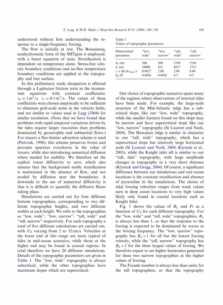
Table 1

Values of topographic parameters

Dimensional

parameter

‘‘low,

wide’’

‘‘low,

narrow’’

‘‘tall,

wide’’

‘‘tall,

narrow’’

h0 (m) 200 200 2350 2350

L (m) 10000 413 4857 1215

g ¼ dh=dxmax=s 0.0827 2.00 2.00 8.00

h0=H 0.0426 0.0426 0.5 0.5


understood without first understanding the re-sponse to a single-frequency forcing.

The flow is initially at rest. The Boussinesq,nonhydrostatic form of the MITgcm is employed,with a linear equation of state. Stratification isdependent on temperature alone. Stress-free velo-city boundary conditions and no-flux temperatureboundary conditions are applied at the topogra-phy and free surface.

In this preliminary study dissipation is effectedthrough a Laplacian friction term in the momen-tum equations with constant coefficients:nh ¼ 1m2=s, nv ¼ 0:1m2=s. The values of thesecoefficients were chosen empirically to be sufficientto eliminate grid-scale noise in the velocity fields,and are similar to values used in Legg (2004) forsimilar resolution. (Note that we have found thatproblems with rapid temporal variations driven bythe tides require larger viscosities than problemsdominated by geostrophic and subinertial flows.)For tracers a flux-limiter advection scheme is used(Pietrzak, 1998); this scheme preserves fronts andprevents spurious overshoots in the value oftracers, while also introducing numerical diffusionwhere needed for stability. We therefore set theexplicit tracer diffusivity to zero, which alsoensures that the background stable stratificationis maintained in the absence of flow, and noteroded by diffusion near the boundaries. Adownside to the use of numerical diffusivity isthat it is difficult to quantify the diffusive fluxestaking place.

Simulations are carried out for four differentbottom topographies, corresponding to two dif-ferent topographic heights, and two differentwidths at each height. We refer to the topographiesas ‘‘low, wide’’, ‘‘low, narrow’’, ‘‘tall, wide’’ and‘‘tall, narrow’’ respectively. For each topography atotal of five different calculations are carried out,with U0 varying from 2 to 32 cm/s. Velocities atthe lower end of this range are more typical oftides in mid-ocean scenarios, while those at thehigher end may be found in coastal regions. Intotal therefore we have 20 different simulations.Details of the topographic parameters are given inTable 1. The ‘‘low, wide’’ topography is alwayssubcritical, while the other topographies havemaximum slopes which are supercritical.

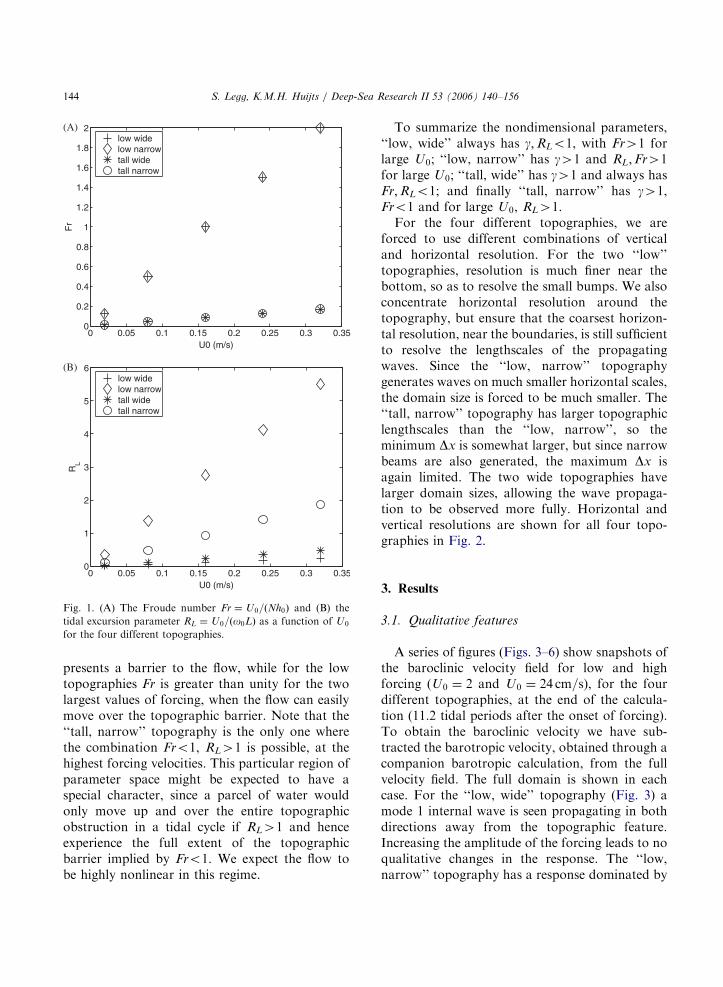
Our choice of topographic scenarios spans manyof the regimes where observations of internal tideshave been made. For example, the large-scalestructure of the Mid-Atlantic ridge has a sub-critical slope, like our ‘‘low, wide’’ topography,while the smaller features found on this slope maybe narrow and have supercritical slope like our‘‘low, narrow’’ topography (St Laurent and Nash,2004). The Hawaiian ridge is similar in characterto our ‘‘tall, wide’’ topography, which has asupercritical slope but relatively large horizontalscale (St Laurent and Nash, 2004; Klymak et al.,2005), while the Knight inlet sill is similar to our‘‘tall, thin’’ topography, with large amplitudechanges in topography in a very short distance(Klymak and Gregg, 2004). Of course, a significantdifference between our simulations and real oceanlocations is the constant stratification and absenceof pycnocline in the simulations. The choice oftidal forcing velocities ranges from weak valuesseen in deep ocean locations to very high valueslikely only found in coastal locations such asKnight Inlet.Fig. 1 shows the values of RL and Fr as a

function of U0 for each different topography. Forthe ‘‘low, wide’’ and ‘‘tall, wide’’ topographies, RL

is always less than 1, so that the response to theforcing is expected to be dominated by waves atthe forcing frequency. The ‘‘low, narrow’’ topo-graphy has RL41 for all but the lowest forcingvelocity, while the ‘‘tall, narrow’’ topography hasRL41 for the three largest values of forcing. Wetherefore expect to see higher harmonics generatedfor these two narrow topographies at the highervalues of forcing.The Froude number is always less than unity for

the tall topographies, so that the topography

ARTICLE IN PRESS

0 0.05 0.1 0.15 0.2 0.25 0.3 0.350

0.2

0.4

0.6

0.8

1

1.2

1.4

1.6

1.8

2

U0 (m/s)

Fr

low widelow narrowtall widetall narrow

0 0.05 0.1 0.15 0.2 0.25 0.3 0.350

1

2

3

4

5

6

U0 (m/s)

RL


(A)

(B)

Fig. 1. (A) The Froude number Fr ¼ U0=ðNh0Þ and (B) the

tidal excursion parameter RL ¼ U0=ðo0LÞ as a function of U0

for the four different topographies.


presents a barrier to the flow, while for the lowtopographies Fr is greater than unity for the twolargest values of forcing, when the flow can easilymove over the topographic barrier. Note that the‘‘tall, narrow’’ topography is the only one wherethe combination Fro1, RL41 is possible, at thehighest forcing velocities. This particular region ofparameter space might be expected to have aspecial character, since a parcel of water wouldonly move up and over the entire topographicobstruction in a tidal cycle if RL41 and henceexperience the full extent of the topographicbarrier implied by Fro1. We expect the flow tobe highly nonlinear in this regime.

To summarize the nondimensional parameters,‘‘low, wide’’ always has g;RLo1, with Fr41 forlarge U0; ‘‘low, narrow’’ has g41 and RL;Fr41for large U0; ‘‘tall, wide’’ has g41 and always hasFr;RLo1; and finally ‘‘tall, narrow’’ has g41,Fro1 and for large U0, RL41.

For the four different topographies, we areforced to use different combinations of verticaland horizontal resolution. For the two ‘‘low’’topographies, resolution is much finer near thebottom, so as to resolve the small bumps. We alsoconcentrate horizontal resolution around thetopography, but ensure that the coarsest horizon-tal resolution, near the boundaries, is still sufficientto resolve the lengthscales of the propagatingwaves. Since the ‘‘low, narrow’’ topographygenerates waves on much smaller horizontal scales,the domain size is forced to be much smaller. The‘‘tall, narrow’’ topography has larger topographiclengthscales than the ‘‘low, narrow’’, so theminimum Dx is somewhat larger, but since narrowbeams are also generated, the maximum Dx isagain limited. The two wide topographies havelarger domain sizes, allowing the wave propaga-tion to be observed more fully. Horizontal andvertical resolutions are shown for all four topo-graphies in Fig. 2.

3. Results

3.1. Qualitative features

A series of figures (Figs. 3–6) show snapshots ofthe baroclinic velocity field for low and highforcing (U0 ¼ 2 and U0 ¼ 24 cm=s), for the fourdifferent topographies, at the end of the calcula-tion (11.2 tidal periods after the onset of forcing).To obtain the baroclinic velocity we have sub-tracted the barotropic velocity, obtained through acompanion barotropic calculation, from the fullvelocity field. The full domain is shown in eachcase. For the ‘‘low, wide’’ topography (Fig. 3) amode 1 internal wave is seen propagating in bothdirections away from the topographic feature.Increasing the amplitude of the forcing leads to noqualitative changes in the response. The ‘‘low,narrow’’ topography has a response dominated by

ARTICLE IN PRESS

-150 -100 -50 0 50 100 1500

200

400

600

800

1000

1200

1400

1600

1800

2000

x (km)

∆ x

(m)


10 20 30 40 50 60

-4500

-4000

-3500

-3000

-2500

-2000

-1500

-1000

-500

0

∆ z (m)

z (m

)


(A)

(B)

Fig. 2. (A) The horizontal resolution Dx as a function of x

(distance from the topographic peak) and (B) the vertical

resolution Dz as a function of z for the four different

topographic scenarios.


the principal frequency at U0 ¼ 2 cm=s, in theform of a narrow beam (Fig. 4A). As theamplitude of the forcing increases, responses athigher harmonics appear: the beam at a steeperangle for U0 ¼ 8 cm=s (Fig. 4B) corresponds to the2o0 internal tide. Unlike Lamb (2004) we do notsee evidence for generation of harmonics bynonlinear wave–wave interactions at the locationswhere beams intersect: all our beams at higherfrequencies can be traced back to the topographyitself. For the tall topographies, upward anddownward propagating beams are seen for U0 ¼

2 cm=s (Figs. 5A, 6A), while at U0 ¼ 24 cm=s thevelocity field near the topography becomes more

disorganized, particularly for the ‘‘tall, narrow’’topography.Closeups of the temperature field at U0 ¼

24 cm=s are shown for all four topographies inFig. 7 at a time of maximum flow to the right. Atlow amplitudes of forcing (not shown) littledeformation of isopycnals is visible. While forthe ‘‘low, wide’’ topography only a small deflectionis produced (Fig. 7A), for the ‘‘low, narrow’’topography (Fig. 7B) the downward plunge of theisopycnals downstream of the topography is muchmore marked. Note that for oscillating flows awater parcel experiences a greater vertical deflec-tion during the tidal period for narrower topo-graphy than for a wider topography of the sameheight. For the tall topographies, a downwardplunge over the ridge is followed by a rebound andsome overturning (Fig. 7C, D), with densityinversions especially visible for the ‘‘tall, narrow’’topography. These snapshots are suggestive oftransient hydraulic behavior, although more rig-orous analysis would be necessary to determinewhether there is truly a transition from subcriticalto supercritical flow.

3.2. Frequency spectra

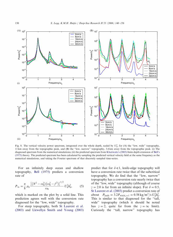
The vertical velocity frequency spectra for all 20simulations are shown in Figs. 8 and 9, scaled byU2

0. Both the spectra diagnosed from the numer-ical simulations and the spectra predicted fromKhatiwala (2003) are shown. Note that the poweris shown on a logarithmic scale so that both largeand small orders of magnitude features are visible,while frequency is shown on a linear scale, since weare interested in highlighting the harmonics, whichcover less than one order of magnitude infrequency. The diagnosed spectra confirm theobservation that the response to the ‘‘low, wide’’topography over the range of velocities studied isapproximately linear—the peak at the forcingfrequency is much larger than that at the higherharmonics, even for the maximum value offorcing. The predicted spectra are very close tothe simulated spectra. For the ‘‘low, narrow’’topography, at U0 ¼ 2 cm=s the largest peak is atthe forcing frequency with successively smallersubsidiary peaks at 2o0, and 3o0. For stronger

ARTICLE IN PRESS

-500

-1000

-1500

z (m

)

x (km)

-2000

-2500

-3000

-3500

-4000

-4500

-150 -100 -50 0 50 100 150

1

0.5

× 10-3

0

-0.5

-1

-1.5

-500

-1000

-1500

z (m

)

x (km)

-2000

-2500

-3000

-3500

-4000

-4500

-150 -100 -50 0 50 100 150

0.015

0.01

0.005

0

-0.005

-0.01

-0.02

-0.015

(A)

(B)

Fig. 3. Snapshots of the baroclinic velocity field (m/s) for the ‘‘low, wide’’ topography, shown for (A) U0 ¼ 2 cm=s and

(B) U0 ¼ 24 cm=s.


forcing the harmonics become more important.Interestingly all higher harmonics have the sameorder of magnitude as the forcing frequency byU0 ¼ 8 cm=s, and not just the first harmonic: againthis agrees with the theoretical prediction. Ourtime sampling is only sufficient to resolve up to afrequency of 4o0, although even higher frequencyresponses may be generated (note thatN=o0 ¼ 5:6, so that propagating waves of fre-quency up to 5o0 are possible), leading to aliasingwhich produces the energy seen at zero frequency.The ‘‘tall, wide’’ topography spectrum again has

a dominant peak at the forcing frequency forU0 ¼ 2 cm=s, and although this frequency con-tinues to dominate, energy is seen at other

frequencies for higher U0. A curious result seenat U0 ¼ 8 cm=s is the peak at 4o0, whichdisappears at higher forcing—the cause of this isunknown. This peak does not appear in thetheoretical result, which predicts only smallharmonic responses for the highest forcing.Additionally, the simulated spectra have muchmore power at intermediate frequencies, betweenthe harmonic peaks, than the theoretical predic-tions.

The ‘‘tall, narrow’’ topography again shows asingle dominant frequency response at U0 ¼

2 cm=s and multiple peaks at the harmonicfrequencies at higher forcing, as predicted fromthe Bell (1975) and Khatiwala (2003) theory.

ARTICLE IN PRESS

-500

-1000

-1500

z (m

)

x (km)

-2000

-2500

-3000

-3500

-4000

-4500

-50 0 50

0.01

-0.01

0.005

-0.005

0

(A)-500

-1000

-1500

z (m

)

x (km)

-2000

-2500

-3000

-3500

-4000

-4500

-50 0 50

0.03

0.02

0.01

0.04

-0.06

-0.05

-0.04

-0.03

-0.02

-0.01

0

(B)

-500

-1000

-1500

z (m

)

x (km)

-2000

-2500

-3000

-3500

-4000

-4500

-50 0 50

0.06

0.04

0.02

0.08

-0.1

-0.08

-0.06

-0.04

-0.02

0

(D)-500

-1000

-1500

z (m

)

x (km)

-2000

-2500

-3000

-3500

-4000

-4500

-50 0 50

0.06

0.04

0.02

0.08

-0.1

-0.08

-0.06

-0.04

-0.02

0

(C)

Fig. 4. Snapshots of the baroclinic velocity field (m/s) for the ‘‘low, narrow’’ topography, shown for (A) U0 ¼ 2 cm=s,(B) U0 ¼ 8 cm=s, (C) U0 ¼ 16 cm=s and (D) U0 ¼ 24 cm=s.


However, the harmonics gain equivalent magni-tude to the forcing frequency peak at somewhatweaker forcing in the simulations compared tothe predictions—this might be attributed to theenhancement of the barotropic flow abovethe topography due to the finite d. Note that inthe spectra diagnosed from the ‘‘tall, narrow’’ andto some extent the ‘‘tall, wide’’ simulations, thepeaks are not discrete; significant energy is foundat frequencies between the no0 harmonics. Thiscontrasts with the spectra from the low topogra-phy simulations or the predicted spectra. Thebroadened peaks could result from Dopplershifting of the internal waves by the mean flow;however, similar Doppler shifting would beexpected for the low topographies, since the

velocities in the deep water where these spectraare obtained are similar, but is absent. Hence thebroadened peaks might indicate the developmentof a continuum such as in a breakdown toturbulence in the tall topography simulations.To summarize these qualitative observations:

the ‘‘low, wide’’ topography produces a linearresponse (a mode 1 internal wave at the forcingfrequency) for all forcing examined here. The‘‘low, narrow’’ topography produces beam-likeinternal waves at progressively more harmonicfrequencies as the forcing is increased. The ‘‘tall,narrow’’ forcing produces a double beam at theforcing frequency for weak forcing, becomingmore disorganized and turbulent, although stillwith energetic peaks at the harmonics of the

ARTICLE IN PRESS

0.6

0.4

0.2

0.8

-0.6

-0.4

-0.2

0

(B)

-500

-1000

-1500

z (m

)

x (km)

-2000

-2500

-3000

-3500

-4000

-4500

-500

-1000

-1500

z (m

)

-2000

-2500

-3000

-3500

-4000

-4500

-50-100-150 0 15010050

x (km)

-50-100-150 0 15010050

0.06

0.04

0.02

-0.12

-0.1

-0.08

-0.06

-0.04

-0.02

0

(A)

Fig. 5. Snapshots of the baroclinic velocity field (m/s) for the

‘‘tall, wide’’ topography, shown for (A) U0 ¼ 2 cm=s and

(B) U0 ¼ 24 cm=s.

0.6

0.4

0.2

0.8

-0.4

-0.2

0

(B)

-500

-1000

-1500

z (m

)

x (km)

-2000

-2500

-3000

-3500

-4000

-4500

-500

-1000

-1500

z (m

)

-2000

-2500

-3000

-3500

-4000

-4500

-50 0 50

-50 0 50

x (km)

0.07

0.08

0.06

0.05

-0.02

-0.01

0.01

0.02

0.03

0.04

0

(A)

Fig. 6. Snapshots of the baroclinic velocity field (m/s) for the

‘‘tall, narrow’’ topography, shown for (A) U0 ¼ 2 cm=s and

(B) U0 ¼ 24 cm=s.


forcing frequency for stronger forcing. The pre-dictions of the frequency of the response made byBell (1975) and Khatiwala (2003) compare wellwith the numerical simulations, except for thebroadening of the peaks in the tall topographysimulations, which we attribute to nonlinearprocesses not accounted for by the theory. In thetheoretical predictions the frequency of the waveresponse is determined by the generation processrather than any subsequent nonlinear wave inter-actions—the agreement between the simulationsand the theory in this respect indicates similarprocesses are responsible for the appearance of theharmonics. Energy transfer between harmonicsdoes not appear to play an important role except

in the transfer of energy to frequencies which arenot tidal harmonics in the tall topography simula-tions.

3.3. Energy conversion and dissipation

Many recent studies have made predictions forthe rate at which energy is converted from thebarotropic to the baroclinic field, and in particularthe changes in this conversion rate introducedby topography of finite steepness g and finiteheight relative to the total depth d (Balmforthet al., 2002; Llewellyn Smith and Young, 2002,2003; Khatiwala, 2003).

ARTICLE IN PRESS

Fig. 7. Snapshots of the temperature field for the four different topographies, shown for U0 ¼ 24 cm=s, at a time of maximum flow

toward the right. Note that both the spatial scales and temperature scales are different in each image: in (A) and (B) we focus on the

bottom 20% of the domain, since finite amplitude displacements are confined to that region because of the small height of the

topography, while in (C) and (D) the full domain height is shown. The displacements in (A) and (B) are much smaller than in (C) and

(D), and would not be visible if the same color scale as in (C) and (D) was used.


We can compare our numerical results with thetheoretical predictions, and also examine the effectof increasing the amplitude of the forcing. Wediagnose the conversion rate in the numericalsimulations as done by Khatiwala (2003):

P ¼

Z x¼Lx

x¼0

p0ðx; z ¼ hðxÞ; tÞUbtðx; tÞdh

dxdx, (3)

where p0ðx; z ¼ hðxÞ; tÞ is the perturbation pressureat the height of the topography, given by

p0ðx; z; tÞ ¼ r0gðZ� ZbtÞ þ pðx; z; tÞ � P0ðzÞ, (4)

where Z is the free-surface elevation, Zbt is the free-surface elevation in a companion barotropic

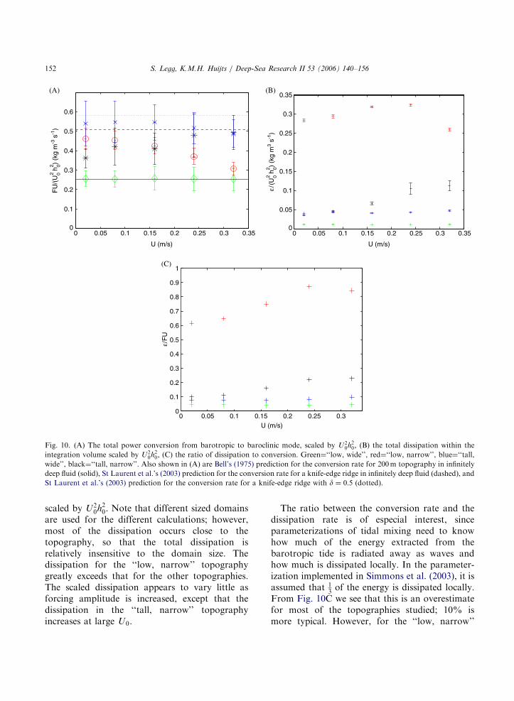
calculation, pðx; z; tÞ is the full pressure (includingnonhydrostatic components) not including thefree-surface contribution, and P0ðzÞ is the hydro-static reference pressure when the fluid is at rest.Ubt is the velocity field from the companionbarotropic calculation, and is not necessarily equalto the forcing velocity when there is largeamplitude topography. The time-averaged conver-sion rate is shown in Fig. 10A for all fourtopographies, along with error bars indicatingthe size of the temporal fluctuations. (The errorbars are not meant to indicate systematic numer-ical errors, which may be unaccounted for.) Allvalues are shown scaled by U2

0h20.

ARTICLE IN PRESS

(A) (B)

(i)

2cm/s8cm/s16cm/s24cm/s32cm/s


(ii)



0 1 2 3 4 510-6

10-5

10-4

10-3

10-2

10-1

100

Frequency/ω0

Pow

er/U

02

0 1 2 3 4 510-4

10-3

10-2

10-1

100

101

Frequency/ω0

Pow

er/U

02

0 1 2 3 4 510-4

10-3

10-2

10-1

100

101

Frequency/ω0

Pow

er/U

02

0 1 2 3 4 510-6

10-5

10-4

10-3

10-2

10-1

100

Frequency/ω0

Pow

er/U

02

Fig. 8. The vertical velocity power spectrum, integrated over the whole depth, scaled by U20, for (A) the ‘‘low, wide’’ topography,

11 km away from the topographic peak, and (B) the ‘‘low, narrow’’ topography, 3.6 km away from the topographic peak. (i) The

diagnosed spectrum from the numerical simulations; (ii) the predicted spectrum from Khatiwala’s (2003) finite depth extension of Bell’s

(1975) theory. The predicted spectrum has been calculated by sampling the predicted vertical velocity field at the same frequency as the

numerical simulations, and taking the Fourier spectrum of that discretely sampled time-series.


For an infinitely deep ocean and shallowtopography, Bell (1975) predicts a conversionrate of

P1 ¼p8r0

N2 � o20

� �o2

0 � f 2� �� 1=2o0

U20h

20, (5)

which is marked on the plot by a solid line. Thisprediction agrees well with the conversion ratediagnosed for the ‘‘low, wide’’ topography.For steep topography, both St Laurent et al.

(2003) and Llewellyn Smith and Young (2003)

predict that for d51, knife-edge topography willhave a conversion rate twice that of the subcriticaltopography. We do find that the ‘‘low, narrow’’topography has a conversion rate nearly twice thatof the ‘‘low, wide’’ topography (although of courseg ¼ 2:0 is far from an infinite slope). For d ¼ 0:5,St Laurent et al. (2003) predict a conversion rate ofabout Pknife ¼ 3:2Pwitch;g¼1 ¼ 0:58 kg=m3=sU2

0h20.

This is similar to that diagnosed for the ‘‘tall,wide’’ topography (which it should be notedhas g ¼ 2, quite far from the g ¼ 1 limit).Curiously the ‘‘tall, narrow’’ topography has

ARTICLE IN PRESS

(A) (B)

(i)



(ii)



0 1 2 3 4 5

Frequency/ω0

Pow

er/U

02

0 1 2 3 4 510-3

10-2

10-1

100

101

102

Frequency/ω0

Pow

er/U

02

0 1 2 3 4 510-3

10-2

10-1

100

101

102

Frequency/ω0

Pow

er/U

02

0 1 2 3 4 510-3

10-2

10-1

100

101

102

10-3

10-2

10-1

100

101

102

Frequency/ω0

Pow

er/U

02

Fig. 9. The vertical velocity power spectrum, as in Fig. 8, but for (A) the ‘‘tall, wide’’ topography and (B) the ‘‘tall, narrow’’

topography, both at a distance of 11 km from the topographic peak.

1Note that this form of the dissipation is equivalent to that in

Tennekes and Lumley (1972) when non-divergence is assumed,

as it is in these simulations, and only those components which

cannot be written as the divergence of a flux are included.


smaller conversion rate than the ‘‘tall, wide’’topography. In contrast, Khatiwala (2003) foundnumerically that the conversion rate increasedmonotonically with g for Gaussian topography;however, he only considered g as high as 1.6,whereas our tall topographies have g ¼ 2 and 8,respectively.

The two ‘‘wide’’ topographies have conversionrates which do not change significantly (afterscaling by U2

0) as the forcing amplitude increases.However, the ‘‘low, narrow’’ topography has ascaled conversion rate which decreases as theforcing increases, so that for the highest amplitudeforcing the conversion rate is nearly the same as

for the ‘‘low, wide’’ topography. By contrast, the‘‘tall, narrow’’ topography has a scaled conversionrate which is less than that of the ‘‘tall, wide’’topography at small amplitude forcing, andincreases as the forcing amplitude increases. Atthe moment we do not have an explanation forthese two differing trends with forcing amplitude.Fig. 10B shows the dissipation rate1

� ¼ niðquj=qxiÞ2, integrated over the volume, and

ARTICLE IN PRESS

0 0.05 0.1 0.15 0.2 0.25 0.3 0.350

0.1

0.2

0.3

0.4

0.5

0.6

U (m/s)

0 0.05 0.1 0.15 0.2 0.25 0.3 0.350

0.05

0.1

0.15

0.2

0.25

0.3

0.35

U (m/s)

0 0.05 0.1 0.15 0.2 0.25 0.30

0.1

0.2

0.3

0.4

0.5

0.6

0.7

0.8

0.9

1

U (m/s)

ε/F

U

FU

/(U

0 h0)

(kg

m-3

s-1

)2

2

ε/(U

0 h0)

(kg

m3 s

-1)

22

(A) (B)

(C)

Fig. 10. (A) The total power conversion from barotropic to baroclinic mode, scaled by U20h20, (B) the total dissipation within the

integration volume scaled by U20h20, (C) the ratio of dissipation to conversion. Green¼‘‘low, wide’’, red¼‘‘low, narrow’’, blue¼‘‘tall,

wide’’, black¼‘‘tall, narrow’’. Also shown in (A) are Bell’s (1975) prediction for the conversion rate for 200m topography in infinitely

deep fluid (solid), St Laurent et al.’s (2003) prediction for the conversion rate for a knife-edge ridge in infinitely deep fluid (dashed), and

St Laurent et al.’s (2003) prediction for the conversion rate for a knife-edge ridge with d ¼ 0:5 (dotted).


scaled by U20h

20. Note that different sized domains

are used for the different calculations; however,most of the dissipation occurs close to thetopography, so that the total dissipation isrelatively insensitive to the domain size. Thedissipation for the ‘‘low, narrow’’ topographygreatly exceeds that for the other topographies.The scaled dissipation appears to vary little asforcing amplitude is increased, except that thedissipation in the ‘‘tall, narrow’’ topographyincreases at large U0.

The ratio between the conversion rate and thedissipation rate is of especial interest, sinceparameterizations of tidal mixing need to knowhow much of the energy extracted from thebarotropic tide is radiated away as waves andhow much is dissipated locally. In the parameter-ization implemented in Simmons et al. (2003), it isassumed that 1

3of the energy is dissipated locally.

From Fig. 10C we see that this is an overestimatefor most of the topographies studied; 10% ismore typical. However, for the ‘‘low, narrow’’

ARTICLE IN PRESS


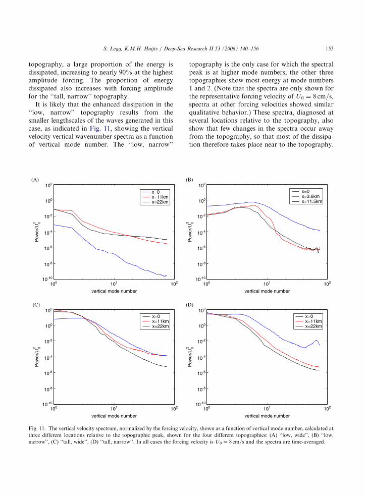
topography, a large proportion of the energy isdissipated, increasing to nearly 90% at the highestamplitude forcing. The proportion of energydissipated also increases with forcing amplitudefor the ‘‘tall, narrow’’ topography.

It is likely that the enhanced dissipation in the‘‘low, narrow’’ topography results from thesmaller lengthscales of the waves generated in thiscase, as indicated in Fig. 11, showing the verticalvelocity vertical wavenumber spectra as a functionof vertical mode number. The ‘‘low, narrow’’

100 101 102

vertical mode number

100 101 102


x=0x=11kmx=22km

x=0x=11kmx=22km

(A)

Pow

er/U

02

10-10

10-8

10-6

10-4

10-2

100

102(

((C)

Pow

er/U

02

10-10

10-8

10-6

10-4

10-2

100

102

Fig. 11. The vertical velocity spectrum, normalized by the forcing velo

three different locations relative to the topographic peak, shown fo

narrow’’, (C) ‘‘tall, wide’’, (D) ‘‘tall, narrow’’. In all cases the forcing

topography is the only case for which the spectralpeak is at higher mode numbers; the other threetopographies show most energy at mode numbers1 and 2. (Note that the spectra are only shown forthe representative forcing velocity of U0 ¼ 8 cm=s,spectra at other forcing velocities showed similarqualitative behavior.) These spectra, diagnosed atseveral locations relative to the topography, alsoshow that few changes in the spectra occur awayfrom the topography, so that most of the dissipa-tion therefore takes place near to the topography.

100 101 102


100 101 102


x=0x=3.6kmx=11.5km

x=0x=11kmx=22km

B)

Pow

er/U

02

10-10

10-8

10-6

10-4

10-2

100

102

D)

Pow

er/U

02

10-10

10-8

10-6

10-4

10-2

100

102

city, shown as a function of vertical mode number, calculated at

r the four different topographies: (A) ‘‘low, wide’’, (B) ‘‘low,

velocity is U0 ¼ 8 cm=s and the spectra are time-averaged.

ARTICLE IN PRESS


3.4. Mixing

We would like to examine how much diapycnalmixing is associated with the dissipation of energyafter the conversion from barotropic to baroclinicflow. Most models of diapycnal mixing (e.g.,Osborn, 1980) assume that a constant fraction ofthe energy dissipated is converted into potentialenergy through mixing. The most direct way toexamine the total mixing therefore is through time-series of total change in potential energy. Weexpect the potential energy to increase in responseto diabatic mixing; however, potential energy alsochanges adiabatically, as dense fluid is pushed upover topography by the flow, or due to passinginternal waves, and hence a time-average overseveral cycles is necessary to obtain an accurateevaluation of the diabatic changes in potentialenergy. Unfortunately the open boundaries intro-duce a further complication—the total heat con-tent is not preserved, due to density changesintroduced at the boundaries. These spuriouschanges in heat content mask the potential energychanges generated by any mixing after a few tidalcycles. Attempts to measure the change inpotential energy in the early part of the calculation(before the heat content changes are significant)were not conclusive due to the large noiseassociated with the tidal cycle. For these reasonsdiagnosing potential energy changes does notallow us to reach any conclusions regarding thediapycnal mixing.The issue of the heat content changes introduced

by the open boundaries makes it difficult to useother diagnostics, e.g., probability density func-tions of density or net changes in stratification, todraw conclusions about the diapycnal mixing.Furthermore, the 2-D nature of the simulationsand the low Reynolds numbers make it likely thatmixing is underestimated in the simulations: forexample, we do not see any evidence for shearinstability in the narrow beams which we mightexpect at higher Reynolds numbers. Additionally,at this resolution the implicit numerical diffusionassociated with the advection scheme is large. Forthis reason, we emphasize that these are prelimin-ary calculations, and further investigation ofthe mixing, involving higher resolution 3-D

calculations will be necessary. These simulationsshould be at a resolution such that numericaldiffusion is minimized compared to explicit diffu-sion. Improvements to the radiative boundaryconditions may also be needed, since thesecurrently appear to perform well in terms ofallowing velocity signals out of the domain, butless well with the density signals, introducingspurious changes in total heat content.

4. Discussion and conclusions

In this survey of parameter space we haveexamined the generation of internal waves anddissipation produced by tidal flow over fourdifferent topographies. The ‘‘low, wide’’ topogra-phy, with subcritical slope, small tidal excursionparameter and large Fr is similar to the overallMid-Atlantic Ridge structure, and leads to thegeneration of linear internal waves dominated bythe forcing frequency and the gravest verticalmode, with a rate of power conversion given byBell (1975) and small dissipation. The ‘‘low,narrow’’ topography is similar in structure to thesmall-scale roughness elements of the MAR, andleads to internal waves with smaller verticalwavelengths and a higher rate of dissipation.The presence of higher modes has indeed beennoted in the observations from the MAR region.St Laurent and Nash (2004) have proposed thatthe dissipation rates in the MAR and HawaiianRidge data can be reconciled by assuming that thedissipation rate depends on the energy content ofthe higher vertical modes, in agreement with oursimulations. An additional feature of the responseof the flow to very narrow topography (i.e. highRL) in the simulations is the appearance of higherharmonic frequencies, as predicted by Bell (1975),but not yet resolved in the observational record.The ‘‘tall, wide’’ topography shows a responsedominated by the gravest vertical mode and theforcing frequency: similar behavior is seen inobservations from the Hawaiian Ridge (Klymaket al., 2005), which has a similar topographicstructure. At the Hawaiian Ridge about 10% ofthe energy converted from the barotropic tide isfound to be dissipated locally—this again agrees

ARTICLE IN PRESS


with our simulations for the ‘‘tall, wide’’ topo-graphy. Finally, the ‘‘tall, narrow’’ topography,which has large RL at the largest magnitudeforcing, develops responses at the higher harmonicfrequencies, with much broader peaks than for the‘‘low, narrow’’ topography. Along with observa-tions of overturning features possibly associatedwith hydraulic jumps, these lead us to believe the‘‘tall, narrow’’ scenario is the most conducive tomixing. Similar hydraulic features have been seenin observations in Knight Inlet (Klymak andGregg, 2004).

The simulations compare well with theoreticalpredictions in many respects: For the ‘‘low, wide’’topography the rate of energy conversion is wellpredicted by Bell (1975), which assumes subcriticalslopes, as in this case. For the supercritical cases,the energy conversion is greater: for the ‘‘low,narrow’’ case it approaches twice the subcriticalvalue, as predicted by St Laurent et al. (2003) andLlewellyn Smith and Young (2003) for a knife-edge ridge. The energy conversion rate for the‘‘tall, wide’’ topography approaches that predictedfor a knife-edge ridge of that height by St Laurentet al. (2003), while that for the ‘‘tall, narrow’’topography is smaller, but increases with forcingamplitude. The appearance of higher harmonics isin general well predicted by the Bell (1975) theory.

From these results we see that the net effect oftidal flow over topography depends not only onthe height of the topography, but also on its widthand its ability to block the flow, as measured by Fr.Narrower topography will lead to higher verticalmodes and greater local dissipation, compared towider topography of the same height or of thesame steepness. Narrow topography that blocksthe flow (high RL combined with low Fr) can leadto hydraulic behavior conducive to overturning,although this scenario is probably found in coastalregions rather than the deep ocean.

These preliminary simulations provide motiva-tion to examine mixing more closely, especially inthe ‘‘tall, narrow’’ and ‘‘low, narrow’’ scenarios,through higher resolution three-dimensional simu-lations. A more detailed study of the mixing mustexamine the dependence of mixing on the model’sdiffusive parameterization and advection scheme.Numerous other parameters, not varied in this

study, such as stratification, tidal frequency(including forcing at multiple frequencies) andCoriolis parameter, may also modify the mixing.

Acknowledgments

K. H. was supported by a Summer StudentFellowship at Woods Hole Oceanographic Institu-tion. S. L. was supported by Office of NavalResearch Grant N00014-03-1-0336 and by awardNA17RJ2612 from the National Oceanic andAtmospheric Administration, US Department ofCommerce. The statements, findings, conclusionsand recommendations are those of the authors anddo not necessarily reflect the views of the NationalOceanic and Atmospheric Administration or theUS Department of Commerce. We thank SamarKhatiwala for sharing his configuration of theMITgcm which served as the starting point forthese simulations. We also thank Jody Klymak,Brian Arbic and Robert Hallberg for their helpfulcomments and suggestions. Comments of threeanonymous reviewers greatly helped to improvethe manuscript.

References

Balmforth, N., Ierley, G., Young, W., 2002. Tidal conversion

by subcritical topography. Journal of Physical Oceanogra-

phy 32, 2900–2914.

Bell, T., 1975. Topographically generated internal waves in the

open ocean. Journal of Geophysical Research 80, 320–327.

Holloway, P., Merrifield, M., 1999. Internal tide generation by

seamounts, ridges, and islands. Journal of Geophysical

Research 108, 25937–25951.

Khatiwala, S., 2003. Generation of internal tides in an ocean of

finite depth: analytical and numerical calculations. Deep-

Sea Research 50, 3–21.

Klymak, J., Gregg, M., 2004. Tidally generated turbulence over

the Knight Inlet Sill. Journal of Physical Oceanography 34,

1135–1151.

Klymak, J., Moum, J., Nash, J.D., Kunze, E., Girton, J.,

Carter, G., Lee, C., Sanford, T., Gregg, M., 2005. An

estimate of tidal energy lost to turbulence at the Hawaiian

Ridge. Journal of Physical Oceanography, in press.

Lamb, K., 2004. Nonlinear interaction among internal wave

beams generated by tidal flow over supercritical topogra-

phy. Geophysical Review Letters 31.

ARTICLE IN PRESS


Legg, S., 2004. Internal tides generated on a corrugated

continental slope. Part II: Along-slope barotropic forcing.

Journal of Physical Oceanography 34, 1824–1834.

Legg, S., Adcroft, A., 2003. Internal wave breaking at concave

and convex continental slopes. Journal of Physical Oceano-

graphy 33, 2224–2246.

Llewellyn Smith, S., Young,W., 2002. Conversion of the barotropic

tide. Journal of Physical Oceanography 32, 1554–1566.

Llewellyn Smith, S., Young, W., 2003. Tidal conversion at a

very steep ridge. Journal of Fluid Mechanics 495, 175–191.

Lvov, Y.V., Polzin, K.L., Tabak, E.G., 2004. Energy spectra of

the ocean’s internal wave field: theory and observations.

Physics Review Letters 92 (12) (Art. No. 128501).

Marshall, J., Adcroft, A., Hill, C., Perelman, L., Heisey, C.,

1997. A finite-volume, incompressible Navier–Stokes model

for studies of the ocean on parallel computers. Journal of

Geophysical Research 102 (C3), 5753–5766.

Munk, W., Wunsch, C., 1998. Abyssal recipes—II: energetics of

tidal and wind mixing. Deep-Sea Research 45, 1977–2010.

Munroe, J.R., Lamb, K., 2005. Topographic amplitude

dependence of internal wave generation by tidal forcing

over idealized three-dimensional topography. Journal of

Geophysical Research 110.

Nash, J., Kunze, E., Toole, J., Schmitt, R., 2004. Internal tide

reflection and turbulent mixing on the continental slope.

Journal of Physical Oceanography 34, 1117–1134.

Nycander, J., 2005. Generation of internal waves in the deep

ocean by tides. Journal of Geophysical Research, 110,

C10028, in press, doi:10.1029/2004JC002487.

Osborn, T., 1980. Estimates of the local rate of vertical

diffusion from dissipation measurements. Journal of Phy-

sical Oceanography 10, 83–89.

Pietrzak, J., 1998. The use of TVD limiters for forward-in-time

upstream-biased advection schemes in ocean modeling.

Monthly Weather Review 126, 812–830.

Polzin, K., 2004. Idealized solutions for the energy balance of

the finescale internal wave field. Journal of Physical

Oceanography 34, 231–246.

Simmons, H., Jayne, S., St Laurent, L., Weaver, A., 2003.

Tidally driven mixing in a numerical model of the ocean

general circulation. Ocean Modelling 6, 245–263.

St Laurent, L., Nash, J., 2004. An examination of the radiative

and dissipative properties of deep ocean internal tides.

Deep-Sea Research 51, 3029–3042.

St Laurent, L., Stringer, S., Garrett, C., Perrault-Joncas, D.,

2003. The generation of internal tides at abrupt topography.

Deep-Sea Research 50, 987–1003.

Tennekes, H., Lumley, J.L., 1972. A First Course in Turbu-

lence.

Zikanov, O., Slinn, D., 2001. Along-slope current generation by

obliquely incident internal waves. Journal of Fluid Me-

chanics 445, 235–261.

http://www.10.1029/2004JC002487

preliminary simulations of internal waves and mixing ... · preliminary simulations of internal...

Documents