Abstract— In this paper, a predictive speed controller (PSC)

based on finite control set model predictive control is developed

for electric drives. The large difference between the mechanical

and electrical time constants necessitates long prediction horizons

for a direct PSC (DPSC) strategy to be implemented. Therefore,

the computation burden for online solving of the optimization

problem critically increases even for low complexity topologies,

whereas the DPSC implementation becomes impossible for high

complexity inverters. Additionally, due to the absence of a PI

controller in DPSC methods, stability issues arise; therefore,

special care is mandated for eliminating steady-state errors. By

using proper weighting of the speed errors, along with the

current errors, in the cost function of the proposed PSC, the use

of many prediction steps becomes unessential. For considering

the current dynamics, a linear controller is incorporated in the

control law of developed PSC offering improved system behavior,

whereas the consideration of the speed errors allows achieving

fast response characteristics. The proposed strategy is

experimentally evaluated through examining reference and

disturbance step changes of a PMSM drive with three-level

neutral-point clamped inverter. Finally, the proposed controller

operation is experimentally compared with a predictive torque

and speed control, by considering several performance indices.

Index Terms—Drive systems, model predictive control,

permanent magnet motors, variable speed drives.

I. INTRODUCTION

ERMANENT magnet synchronous motor (PMSM) drives

have been widely adopted in industrial applications thanks

to their high efficiency and high power density. Two of the

most common strategies employed for the control of PMSM

drives are direct torque control (DTC) and field-oriented

control (FOC) [1], [2]. As the complexity of the inverter

topology increases, the specifications of the electric drive

become more demanding and additional control objectives are

forced to be satisfied for high performance operation. For

example, when neutral-point clamped (NPC) inverters are

adopted, special care is given on the neutral-point potential

balance and on the distribution of the switching losses [3]–[5].

The high complexity of such a system necessitates the use of

This work was made possible by the PDRA award [PDRA 2-1110-14066]

from the Qatar National Research Fund (a member of The Qatar Foundation).

The statements made herein are solely the responsibility of the authors.

The authors are with the Department of Electrical and Computer Engineering, Texas A&M University at Qatar, Doha 23874, Qatar (email:

panagiotis.kakosimos@qatar.tamu.edu, haitham.abu-rub@qatar.tamu.edu)

advanced control strategies that are capable of considering

multi-variable systems [6], [7].

In such cases, model predictive control (MPC) becomes a

favorable choice toward enhancing system performance [2],

[8]–[11]. Two of the most widely used MPC strategies in

electric drives are predictive torque control (PTC) and direct

predictive speed control (DPSC). The inclusion of constraints

and nonlinearities in the control law of MPC is straightforward

which offers a superior advantage of MPC over its

counterparts [12]–[14]. More specifically, a comparative study

between FOC and PTC of an induction motor (IM) drive with

a 2L-VSI has been presented in [9]. The study showed that

PTC achieves comparable steady-state results but with faster

dynamic response and less speed oscillations. However, due to

the absence of a modulator, the switching frequency of MPC

is variable and usually lies in the range of some kHz, thus

hindering its use in applications where high switching

frequency is desirable. Nevertheless, as discussed in [1], [9],

the computation capacity of microprocessors is ever

increasing, making the use of MPC possible in applications

where conventional practices prevail. Furthermore, the

multivariable nature of MPC enabled the controller to

minimize the speed ripple in [15], whereas in [16], the PTC

successfully tracked the maximum torque per ampere

trajectory of an interior PMSM overcoming the high saliency

levels. In the aforesaid cases ([6], [9], [16]–[18]), predictive

control was accompanied by a proportional-integral (PI)

controller.

On the other hand, several DPSC strategies have been

presented in literature. A DPSC strategy directly controls the

speed of the motor and achieves high-speed control dynamics.

More specifically, a PMSM drive system was controlled by a

cascade-free predictive controller exhibiting fast response to

speed changes in [8]. In [19], DPSC was used along with an

optimization algorithm achieving good dynamic behavior

while keeping all the system variables within their normal

operating range. A DPSC was developed for a two-mass

system in [20] mitigating torque pulsations by penalizing

switching states that generate high frequencies in the phase

currents. In [21], the use of an augmented state-space model

combining current and speed control exhibited promising

characteristics. All the aforementioned examples of direct

MPC are favored by its nature allowing the consideration of

several system constraints while meeting strict specifications.

However, the large difference between the mechanical and

electrical time constants necessitates long prediction horizons

Predictive Speed Control with Short Prediction

Horizon for Permanent Magnet Synchronous

Motor Drives

Panagiotis Kakosimos, Member, IEEE, and Haitham Abu-Rub, Senior Member, IEEE

P

for the DPSC strategy to be implemented for electric drives

[8]. The high computation burden of solving the optimization

problem in real time hinders the implementation of the DPSC

method even in conventional voltage-source inverters (VSIs)

and requires simplifications of the involved components [5],

[17], [18]. Therefore, alternative approaches, or even

compromises, are considered, while the use of switching state

minimization techniques becomes of high importance [22],

[23]. Additionally, the absence of a PI controller raises

concerns about the system stability, whereas the elimination of

steady-state errors is difficult and demands additional control

routines. Without integral action or without a PI controller,

direct MPC faces challenging performance issues; thus,

special care was given in [24]. It is evident that although

DPSC offers improved transient performance, its

implementation faces critical performance issues and

challenges.

In this paper, the aforementioned problems are addressed by

weighting both the speed and current errors in the cost

function of the proposed PSC; therefore, the developed finite-

control set (FCS)-MPC combines the advantages of both

indirect and direct predictive control schemes. More

specifically, the use of many predictions steps is not mandated

because the current errors, which are provided by an

incorporated PI controller in the control law of MPC, are

involved in the decision process. Additionally, the use of an

indirect scheme enables the controller to improve the overall

system performance by eliminating steady-state errors and

mitigating high-frequency current components. On the other

hand, the consideration of the speed errors offers improved

behavior when encountering abrupt transient conditions.

Hence, the developed controller achieves a performance

similar to that of DPSC strategies but with short prediction

horizon, low computation burden, and improved steady-state

characteristics. In order to assess the performance of the

developed PSC, a PMSM drive with a 3L-NPC inverter is

investigated, where the high number of output voltage vectors

significantly increases the challenge for the controller. The

proposed PSC method is experimentally evaluated by

examining the steady-state and dynamic performance under

speed and load torque changes of the electric drive. The

proposed controller is experimentally compared with PTC and

PSC strategies in terms of several quantitative and qualitative

performance indices and control objectives.

II. MOTOR AND INVERTER DYNAMIC MODEL

The design characteristics of a PMSM significantly differ

from that of the widely used IMs. It is characterized with

increased challenges for the control system. The predictive

model has to be developed in such a manner that a dynamic

control is accomplished, while the restrictions arising from the

inverter topology are addressed. An overview of the

considered system topology is shown in Fig. 1.

A. State-space model

The well-known electrical PMSM state-space model is used

by the controller to estimate the value of the system state-

space variables at the end of future sampling instants [5], [25].

For the convenience of programming, the system equations are

expressed in matrix form as follows:

𝑑𝑥

𝑑𝑡= 𝐀𝑥 + 𝐁𝑢 + 𝐸, (1)

where the state vector is 𝑥 = 𝑦 = [𝑖𝑑 , 𝑖𝑞]𝑇. The system

matrices used in (1) are:

𝐀 = [−

𝑅

𝐿𝑑

𝐿𝑞

𝐿𝑑𝜔

−𝐿𝑑

𝐿𝑞𝜔 −

𝑅

𝐿𝑞

] , 𝐁 = [

1

𝐿𝑑0

01

𝐿𝑞

] , 𝐄 = [0

−𝜓

𝐿𝑞𝜔], (2)

where 𝑅 is the stator resistance, 𝐿𝑑 and 𝐿𝑞 are the dq-axis

inductances, 𝜔 is the electrical speed and 𝜓, is the flux linkage

established by the permanent magnets. Since the directly

controlled variables are the dq-axis motor currents, the output

vector, 𝑦, is identical with the state vector, 𝑥. The control

vector, 𝑢 = [𝑢𝑑, 𝑢𝑞]𝑇 = 𝐌𝐃𝐔 associates the switching states

with the predicted values of the controlled variables. Because

the switching-state vector, 𝐔, is expressed in the three-phase

representation system {�⃗�, �⃗⃗�, 𝑐}, the conversion matrices 𝐌 and

𝐃 are used to transform it into the αβ-frame {�⃗�, 𝛽} and

afterwards into the dq-reference frame {𝑑, �⃗�} as follows:

𝐌 = [𝑠𝑖𝑛𝜃 −𝑐𝑜𝑠𝜃𝑐𝑜𝑠𝜃 𝑠𝑖𝑛𝜃

] , 𝐃 =2

3[1 − 1 2⁄ − 1 2⁄

0 √3 2⁄ −√3 2⁄], (3)

where 𝐔 is 𝐔 = [Γ𝑎, Γ𝑏 , Γ𝑐]𝑇 and 𝜃 is the electrical angle of

the rotor. Parameter Γ can be expressed as function of the DC-

link capacitor voltages and the switching state, 𝑇, as next:

Γ𝑥 =𝑇𝑥(𝑇𝑥 + 1)

2𝑣𝐶1 −

𝑇𝑥(𝑇𝑥 − 1)

2𝑣𝐶2. (4)

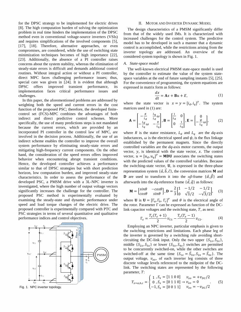
Employing an NPC inverter, particular emphasis is given to

the switching restrictions and limitations. Each phase leg of

the inverter is governed by a switching rule avoiding short-

circuiting the DC-link input. Only the two upper {𝑆1𝑥 , 𝑆2𝑥},

middle {𝑆2𝑥 , 𝑆3𝑥} or lower {𝑆3𝑥 , 𝑆4𝑥} switches are permitted

to be concurrently switched-on, while the other switches are

switched-off at the same time {𝑆1𝑥 = 𝑆3̅𝑥 , 𝑆2𝑥 = 𝑆4̅𝑥}. The

output voltage, 𝑣𝑥𝑜, of each inverter leg consists of three

discrete voltage levels referenced to the midpoint of the DC-

link. The switching states are represented by the following

parameter, 𝑇:

𝑇𝑥=𝑎,𝑏,𝑐 = {10

−1

, 𝑆𝑥 = [1 1 0 0]

, 𝑆𝑥 = [0 1 1 0]

, 𝑆𝑥 = [0 0 1 1]→

𝑣𝑥𝑜 = +𝑣𝐷𝐶/2𝑣𝑥𝑜 = 0 𝑣𝑥𝑜 = −𝑣𝐷𝐶/2

. (5)

Fig. 1. NPC inverter topology.

At the end of the prediction stage of the motor currents, the

electromagnetic torque can be estimated by using:

𝑇𝑒𝑛 =3

2𝑝(𝜓𝑖𝑞 + (𝐿𝑑 − 𝐿𝑞)𝑖𝑑𝑖𝑞). (6)

For extending the controller to control the speed directly, the

mechanical state-space model is used. The electrical motor

speed is given by the following differential equation:

𝑑𝜔

𝑑𝑡= −

𝐵𝑣

𝐽𝑚

𝜔 +𝑝

𝐽𝑚

(𝑇𝑒𝑛 − 𝑇𝑙), (7)

where 𝑝 is the number of pole pairs and 𝑇𝑙 is the load torque.

Parameters 𝐵𝑣 and 𝐽𝑚 are the moment of inertia and damping

ratio, respectively.

B. Neutral-point potential balance

The voltage balance, 𝑣𝑁𝑃, across the terminals of the DC-

link capacitors is achieved by regulating the time of which

each inverter leg dwells on the middle point, 𝑜. Voltage

unbalance is undesirable because it has an immediate negative

effect on the output voltage and on the semiconductor switch

stress. Enabling the controller to consider such unbalance is

possible by expressing the voltage difference of the capacitors

as function of the switching states. In literature, several

methods exist for keeping the voltage of the neutral point at

zero level [26]. In order for the MPC to minimize the voltage

difference, 𝑣𝑁𝑃, by predicting it at the end of the next

sampling period, the sensing of the DC input current, 𝑖𝐷𝐶 , or

the currents of the capacitors, 𝑖𝐶𝑥, is mostly used [27], [28].

However, the potential of the neutral point can be predicted by

measuring only the total DC-link voltage and not the

individual voltages of the capacitors [29]. This helps in

decreasing the component count and improving system

reliability. The current flowing from the middle point of the

DC-link to the clamping diodes, 𝑖𝑁𝑃, can be expressed by:

𝑖𝑁𝑃 = [1 − 𝑇𝑎2 1 − 𝑇𝑏

2 1 − 𝑇𝑐2]𝐢, (8)

where 𝐢 = [𝑖𝑎, 𝑖𝑏 , 𝑖𝑐]𝑇. The voltage difference of the DC-link

capacitors, 𝑣𝑁𝑃, can be estimated by using the differential

equation that describes their operation:

𝑖𝐶1 − 𝑖𝐶2 = 𝐶𝑑

𝑑𝑡(𝑣𝐶2 − 𝑣𝐶1) → 𝑖𝑁𝑃 = 𝐶

𝑑𝑣𝑁𝑃

𝑑𝑡. (9)

Considering (8) and (9), the voltage unbalance is expressed

as a function of the switching states. In (9), both capacitances

have been considered equal 𝐶1 = 𝐶2 = 𝐶.

III. PROPOSED PREDICTIVE CONTROLLER

By using the dynamic inverter and motor model and by

evaluating all the possible switching combinations, the

predictive controller can decide which combination satisfies

all the set requirements with minimum cost. However, since

the control strategy is implemented into a digital controller,

the continuous-time model needs to be discretized first. In

electric drives, several discretization methods have been used

in order to find an accurate discrete-time model. When the

computation burden is a concern, simple discretization

methods are usually adopted [9], [16], [30]. However, when a

highly time-consuming method is applied, the system

accuracy can be significantly increased [17], [19], [31]. In this

study, the computation load is high because of the high

number of switching states. Therefore, the approach based on

Euler discretization in [24] has been found favorable while

offering satisfactory performance.

In conventional cascade-free PSC strategies [8], the speed,

𝜔𝑚, is estimated using the speed dynamics (7) and is

compared with the reference speed, 𝜔𝑚∗ . Owing to the large

difference between mechanical and electrical time constants, a

long prediction horizon is mandated in the prediction process

of the speed [8], [21]. However, in the case where a 3L-VSI is

employed, the number of the switching combinations becomes

high enough, making the implementation of direct speed

controller a challenge. Regardless the number of prediction

steps, integrators are needed to provide the speed reference

and advanced observers to compensate parameter variation

and model inaccuracy [20], [21]. When the implementation of

a DPSC is difficult due to aforementioned reasons, good

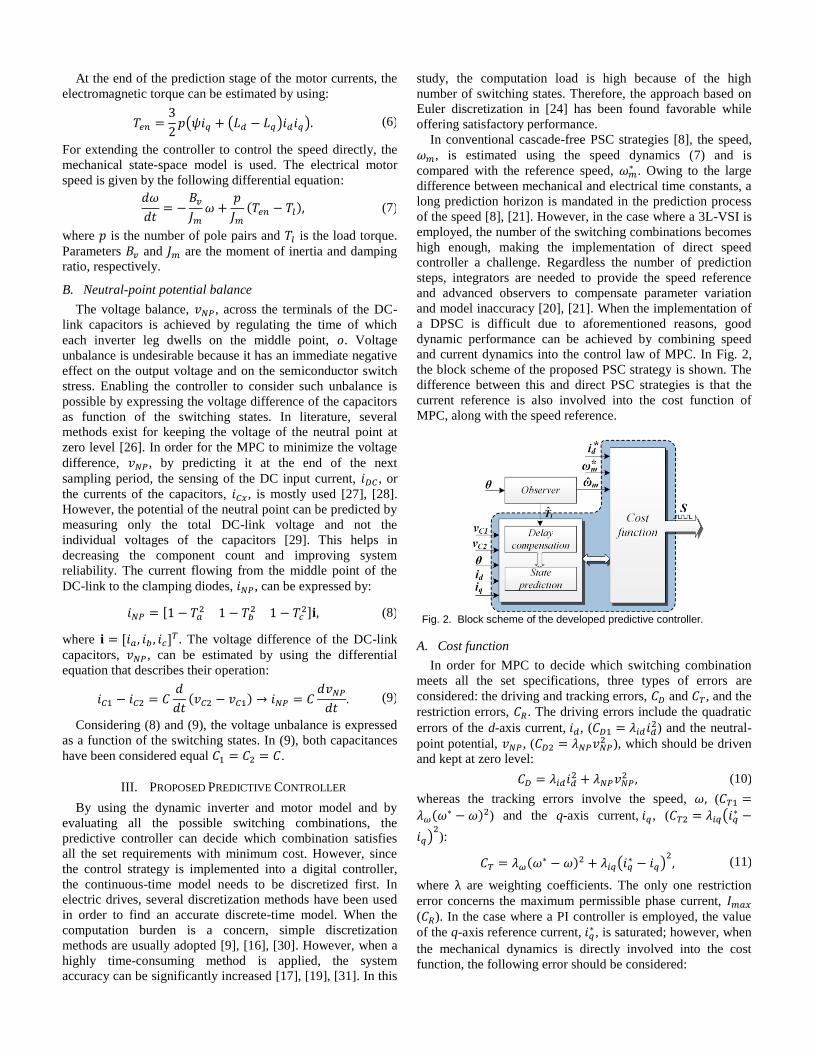
dynamic performance can be achieved by combining speed

and current dynamics into the control law of MPC. In Fig. 2,

the block scheme of the proposed PSC strategy is shown. The

difference between this and direct PSC strategies is that the

current reference is also involved into the cost function of

MPC, along with the speed reference.

A. Cost function

In order for MPC to decide which switching combination

meets all the set specifications, three types of errors are

considered: the driving and tracking errors, 𝐶𝐷 and 𝐶𝑇, and the

restriction errors, 𝐶𝑅. The driving errors include the quadratic

errors of the d-axis current, 𝑖𝑑, (𝐶𝐷1 = 𝜆𝑖𝑑𝑖𝑑2) and the neutral-

point potential, 𝑣𝑁𝑃, (𝐶𝐷2 = 𝜆𝑁𝑃𝑣𝑁𝑃2 ), which should be driven

and kept at zero level:

𝐶𝐷 = 𝜆𝑖𝑑𝑖𝑑2 + 𝜆𝑁𝑃𝑣𝑁𝑃

2 , (10)

whereas the tracking errors involve the speed, 𝜔, (𝐶𝑇1 =

𝜆𝜔(𝜔∗ − 𝜔)2) and the q-axis current, 𝑖𝑞 , (𝐶𝑇2 = 𝜆𝑖𝑞(𝑖𝑞∗ −

𝑖𝑞)2):

𝐶𝑇 = 𝜆𝜔(𝜔∗ − 𝜔)2 + 𝜆𝑖𝑞(𝑖𝑞∗ − 𝑖𝑞)

2, (11)

where λ are weighting coefficients. The only one restriction

error concerns the maximum permissible phase current, 𝐼𝑚𝑎𝑥

(𝐶𝑅). In the case where a PI controller is employed, the value

of the q-axis reference current, 𝑖𝑞∗ , is saturated; however, when

the mechanical dynamics is directly involved into the cost

function, the following error should be considered:

Fig. 2. Block scheme of the developed predictive controller.

𝐶𝑅 = {𝜆𝐼𝑚 (√𝑖𝑑

2 + 𝑖𝑞2 − 𝐼𝑚𝑎𝑥) ,

0,

𝑖𝑓 √𝑖𝑑2 + 𝑖𝑞

2 > 𝐼𝑚𝑎𝑥 ,

𝑜𝑡ℎ𝑒𝑟𝑤𝑖𝑠𝑒.

(12)

In conventional DPSC, the tracking errors in (11) involve

only the dynamics of the speed without considering the current

errors. In this case, a long prediction horizon is needed to

compensate for the difference in mechanical and electrical

dynamics. At steady-state operation, when the motor reaches

the reference speed, the speed error in the cost function is

expected to be significantly low because the mechanical time

constant is considerably larger than the sampling time. If the

prediction horizon is not high enough in order to involve both

dynamics, high-frequency components are generated in the

motor currents [20]. In order to mitigate these components, the

integral function of a linear controller is incorporated into the

cost function of the predictive controller in (11):

𝑖𝑞∗ [𝑘] = 𝑖𝑞

∗ [𝑘 − 1] + 𝑘1(𝜔∗[𝑘] − 𝜔[𝑘])

+ 𝑘2(𝜔∗[𝑘 − 1] − 𝜔[𝑘 − 1]), (13)

where 𝑘1 and 𝑘2 are the coefficients of the linear controller.

The current errors (𝐶𝑇2) which involve the generated q-axis

reference current, 𝑖𝑞∗ , are weighted in the cost function of PSC.

Switching combinations that generate high frequencies in the

phase currents are penalized because their current errors (𝐶𝑇2)

are large. On the other hand, under speed transients, the

behavior of the controller is similar to that of DPSC strategies.

The speed errors (𝐶𝑇1) are high enough because of the large

difference between the reference, 𝜔∗, and actual speed, 𝜔.

The parameters of the linear controller can be calculated by

using the pole-assignment method along with the feedforward

controller structure and considering only the mechanical

dynamics [24]. Therefore, the first-order model of the motor is 𝛺(𝑠)

𝐼𝑞∗(𝑠)

≈𝑏

𝑠+𝑎 and the gains can be computed by:

𝑘 =2𝜉𝜔𝑛 − 𝑎

𝑏, 𝜏 =

2𝜉𝜔𝑛 − 𝑎

𝜔𝑛2

, (14)

where 𝜏 is the integral time constant, 𝑘 is the proportional

gain, 𝜉 is the damping coefficient and 𝜔𝑛 is the natural

frequency. The 𝑘1 coefficient is equal to the proportional gain,

𝑘, whereas the 𝑘2 coefficient is 𝑘 (−1 +𝑇𝑠

𝜏). It is important to

note that the first-order model is independent of the electrical

parameters of the motor. The parameters 𝑎 and 𝑏 in (14) are

𝑎 =𝐵𝑣

𝐽𝑚, 𝑏 =

3

2

𝑝2𝜓

𝐽𝑚α [24].

The combination of both dynamics allows the controller to

differentiate its behavior depending on the operating

condition. The use of long prediction horizons is not

mandated, and the algorithm can be implemented even for

topologies with high complexity. The total switching states of

a 3L-NPC inverter are 27, 8 of which are redundant. There are

four discrete categories of voltage vectors: 3 zero vectors

{𝑣1 … 𝑣3}, 12 small vectors {𝑣4 … 𝑣15}, 6 medium vectors

{𝑣16 … 𝑣21}, and 6 large vectors {𝑣22 … 𝑣27}. Since the

number of voltage vectors is high enough, the computation

burden is thus significantly increased and in some cases, the

consideration of long prediction horizons is impossible. For

reducing the number of the examined switching states, and

consequently the total burden, several methods have been

presented in literature [8], [16].

Furthermore, predictive control employs weighting factors,

λ, in the decision process allowing system variables of

different nature to be controlled as in (10)-(12). The

determination of the weighting coefficients is a challenging

process, which is usually based on empirical or heuristic

methods. Since the controlled variables are expressed in

different units, the primary use of the weights is to normalize

the errors involved in the cost function. In order to determine

their values, the performance of the controller is tested under

several test-case scenarios considering satisfactory

performance characteristics and the satisfaction of the system

restrictions. Finally, the cost function for the evaluation of the

switching states takes the following form:

𝑔 = ∑ 𝐶𝐷𝑚

2

𝑚=1

+ ∑ 𝐶𝑇𝑛

2

𝑛=1

+ 𝐶𝑅. (15)

B. Load torque observer

In order for the controller to predict the motor speed in (7),

the load torque information is necessary; therefore, an

extended Luenberger observer has been adopted. The use of a

load torque observer allows estimating the torque without

using additional sensing equipment. The estimated load

torque, along with the estimated speed, has been designated as

input to the controller as shown in the block scheme of Fig. 2.

It is worth noticing that the impact of the speed measurement

noise, owing to the quantization of the mechanical angle may

significantly affect the system performance given the high

sampling rate of the predictive controller. Therefore, the

observer not only assists in providing the load torque

information for the controller, but also helps in mitigating

noise and discretization errors from the speed sensor. The load

torque and speed observer is designed as follows:

𝑑�̂�

𝑑𝑡= 𝐀�̂� + 𝐁�̂� + 𝐋𝑣, (16)

where 𝑥 = [𝜃, 𝜔, 𝑇𝑙]𝑇, 𝑣 = 𝑦– �̑� = 𝑪(𝑥– �̑�) and 𝑳 =

[𝑙1, 𝑙2, 𝑙3]𝑇. Hereafter, the notation ( ̂) is used for the

description of estimated values. The system matrices 𝐀 and 𝐁

derive from the mechanical dynamics in (7). By regulating the

gains of the observer, its response can be properly adjusted

[8]. Both the observer and the predictive controller are

sensitive to the deviations of the moment of inertia. The inertia

identification of a single or two-mass system is a difficult

process. In literature, there are approaches where the inertia is

updated based on the on-line self-tuning of the observer (16).

In this paper, the moment of inertia, 𝐽𝑚, and the damping ratio,

𝐵𝑣, of the experimental setup have been identified by carrying

out extensive experiments.

IV. EXPERIMENTAL SETUP & SYSTEM SPECIFICATIONS

In order to validate the performance of the developed

methodology experimentally, an experimental setup was

employed. In this setup, a surface-mount PMSM is supplied

by a three-phase NPC inverter and is coupled to a hysteresis

brake by a spring shaft coupling. The brake is equipped with

its own controller board and is capable of providing

programmable torque loading independent of the shaft speed.

Table I summarizes the main characteristics of the test-bed.

The control algorithm, which is written in C language, is

implemented on a dSPACE PX10 expansion box equipped

with a DS1006 processor. The processor board is accompanied

by a high-speed A/D board, a digital output board, and an

incremental encoder interface board. For configuring the

parameters of the examined controllers, Controldesk

experiment software is used. The main controller board

receives and processes the signals from the current and voltage

transducers as well as the pulse series generated by the speed

encoder. The circuit connections of the investigated system are

shown in the block diagram of Fig. 3 whereas Fig. 4 depicts

the experimental setup used for the validation of the developed

control strategy. TABLE I

MAIN SYSTEM PARAMETERS

Motor parameter / Symbol

Value System parameter /

Symbol Value

Dq-axis inductances, 𝐿 20 mH Nominal torque, 𝑇 10 Nm

Nominal current, 𝐼𝑁 2.7 A Nominal speed, 𝜔𝑚 20 rad/s

Winding resistance, 𝑅 6.98 Ω DC-link capacitors, 𝐶 3 mF

Flux linkage, 𝜓 1.06 Wb DC-bus voltage, 𝑣𝐷𝐶 400 V

Pole pairs, 𝑝 4 Moment of inertia, 𝐽𝑚 0.0212 kgm2

Voltage constant, 𝑘𝑒 750 Vp/krpm Viscous damping, 𝐵𝑣 3.1·10-4 Nms

A quadrature speed encoder with a resolution of 2048

pulses per revolution is used. The low resolution of the speed

encoder demands a special attention in order to avoid

discretization errors in cases where the motor speed is low and

the sampling frequency of the controller is high. The

maximum motor speed is limited by the voltage of the DC

bus. The high computation resources needed for the processor

to implement the control strategies determine the finally

applied switching frequency range. The sampling time for the

developed PSC strategy is found approximately 80μs. A delay

compensation stage is also considered for compensating the

computation time delay caused by the digital controller.

Furthermore, in order to use the same baseline for the

comparison of different control techniques, the same sampling

time is adopted. The average switching frequency of the

predictive controllers is identified in the range of 1-2 kHz.

V. CONTROLLER EVALUATION

The developed PSC strategy is evaluated by examining the

operation of the drive system either under normal or abrupt

transient operating conditions. The controller performance is

also compared with the performance of PSC strategy with

filtering the high-frequency current components (PSCf) [20],

and conventional PTC [16] by conducting several simulations

and experiments. For determining the initial gain values, the

pole-assignment design technique has been employed for both

PTC and PSC strategies, and a preliminary study has been

conducted with the damping coefficient, 𝜉, equal to 0.707.

This damping coefficient has been selected because it allows

fast speed response with a reasonable overshoot and improved

disturbance rejection. However, after specifying the initial

gains, several tests have been carried out to tune their values.

It has been found that when the proportional gain of the PI

controller is 0.60 (= 𝑘) with a time constant of 0.028 (= 𝜏),

the transient behavior of the controller is satisfactory and the

system remains stable when encountering disturbances. In

order for the comparison of the PTC and PSC strategies to be

fair, the coefficients in (13) were calculated by discretizing the

PI controller parameters of PTC; thus, equivalent gains are

used for the suggested PSC (𝑘1=𝑘=0.60, 𝑘2= 𝑘 (−1 +

𝑇𝑠

𝜏)=−0.598).

On the other hand, for the determination of the weighting

coefficients, 𝜆, extensive experiments have been carried out

enabling the system to perform satisfactorily at steady-state

conditions as well as under dynamic changes. The weights for

the current errors are firstly determined by normalizing their

values; therefore, the initial values are 𝜆𝑖𝑞 = 𝜆𝑖𝑑 =1

𝐼𝑁.

Secondly, the weight of the neutral-point potential is

determined in order to ensure that the controller keeps the

voltage difference of the DC-link capacitors within the

required limits. Afterward, the additional weighting factor of

the speed errors is calculated for achieving improved transient

response without distorting the motor currents. Finally, the

derived weighting factors have been tuned by conducting a

sensitivity analysis and adopted for all the examined

predictive control strategies (𝜆𝑖𝑞=0.25, 𝜆𝑖𝑑=0.25, 𝜆𝜔=10,

𝜆𝑁𝑃=0.1, 𝜆𝐼𝑚=106). Finally, the gains of the developed

observer for the proposed PSC as well as PSCf are 105 (= 𝑙1),

2x104 (= 𝑙2) and 5x102 (= 𝑙3).

For the implementation of the PSCf strategy [20] used for

the experimental assessment of the developed controller, the

same configuration parameters are adopted. In this method,

the switching states that generate high frequency components

in the phase currents are penalized. Therefore, in the driving

Fig. 3. Block diagram of the experimental setup.

Fig. 4. Experimental setup.

errors, 𝐶𝐷, of (15), one additional control requirement needs to

be considered [20]:

𝐶𝐷3 = 𝜆𝑖𝑞𝑖𝑞𝑓2 + 𝜆𝑖𝑞

′ (𝜔∗ − 𝜔)𝑖𝑞𝑓′2 , (17)

where 𝑖𝑞𝑓 and 𝑖𝑞𝑓′ are the filtered versions of the q-axis

current. The purpose of these two additional terms is to keep

the high frequency components of the q-axis current at zero

level. However, this strategy entails increased computation

resources mainly due to the addition of the two discrete filters

into the online prediction process. Moreover, the

determination of the weighting factors along with the cut-off

frequencies of both filters is not a straightforward process.

These additional parameters can be determined by conducting

several experiments while assessing the system performance.

It has been found that when the cut-off frequency of the filters

is around 500 Hz and the additional weighting factor is 𝜆𝑖𝑞′ =

𝜆𝑖𝑞10−2 , the controller effectively handles the drive system.

Furthermore, both simulations and experiments have the

same system parameters such as gains, weighting factors,

observer characteristics, and sampling rates allowing safe

conclusions. However, the aforementioned parameters can be

further fine-tuned in the experimental setup. At this point, two

important differences have to be noted. Firstly, in the

simulation model, a single-mass system has been considered,

whereas in the experimental setup a two-mass system is

employed. The used hysteresis brake has its own PI controller

in order to regulate the applied load torque. Secondly, the low

resolution of the speed encoder, quantization errors, offset,

and linearity errors in the transducers are expected to have

negative impact on the performance of the experimental

system.

A. Simulation results

The performance of the drive system is evaluated by

considering several successive operating conditions involving

speed reference and loading changes for the three examined

control strategies. The purpose of these simulations is to

examine the dynamic performance of the developed controller

highlighting the aspects that cannot be tested experimentally.

1) Steady-state and transient operation

As shown in Fig. 5a, the motor starts from standstill and its

speed reverses at 𝑡 = 0.2 and 0.4 s under a load torque of 10

Nm. Afterward, at 𝑡 = 0.6 s, the load torque changes from 10

to 1 Nm and recovers at 𝑡 = 0.8 s. The reference speed and

load torque used to produce the simulation results of Fig. 5a

are shown in Fig. 5b. In order not to violate the maximum

permissible phase current, all controllers are saturated at 1.5

times the nominal current.

TABLE II

RESPONSE CHARACTERISTICS OF FIG. 6A AND B

Time, 𝑡 (s) 0.2 (a) 0.4 (b)

Parameter / Method PSC PTC PSCf PSC PTC PSCf

Rise time, 𝑡𝑟 (ms) 13.6 16.5 13.6 21.1 26.8 21.7

Settling time, 𝑡𝑆𝑆 (ms) 17.2 52.9 19.4 27.05 58.08 29.45

Over/under shoot, 𝑂𝑉 (%) 1.34 6.66 6.98 0.854 4.56 4.47

Peak, 𝑛𝑝 (rpm) 195.1 205.5 206.2 192.63 199.71 199.55

Peak time, 𝑡𝑝 (ms) 20.5 37.0 18.5 30.5 50.4 29.1

The dynamic and steady-state performance of the three

methods is satisfactory. As shown in Fig. 6, the developed

PSC strategy has the lowest overshoot in the four transient

conditions with minimum settling time and exhibits a

significantly improved dynamic performance. Although the

gains of the controllers of the proposed PSC and the

conventional PTC have the same configuration, the overshoot

of the latter method is significantly higher. By comparing

these two methods it is evident that when the speed dynamics

are included into the control law of MPC, the system

performance is enhanced and it is similar to that of DPSCs but

with short prediction horizon and consequently less

computation burden. During the speed change, the speed error

is high compared to the current error, thus the controller

accurately tracks the speed reference. At steady-state

operation, both methods exhibit similar performance because

the speed error for all the switching states is significantly

smaller. In this case, the current error drives the decision

process of PSC mitigating the high frequency components in

the phase currents.

TABLE III

RESPONSE CHARACTERISTICS OF FIG. 6C AND D

Time, 𝑡 (s) 0.6 (c) 0.8 (d)

Parameter / Method PSC PTC PSCf PSC PTC PSCf

Over/under shoot, 𝑂𝑉 (%) 11.3 18.1 10.9 10.7 18.3 10.2

Peak, 𝑃 (rpm) 212.6 225.6 210.3 170.5 156.2 171.9

Peak time, 𝑡𝑝 (ms) 9.9 13.9 9.6 9.5 15.1 9.2

On the other hand, the performance of the PSCf method is

also satisfactory at steady-state conditions and under load

torque changes. However, during speed transient conditions

the added filters negatively affect the performance of the

controller by increasing the overshoot and oscillations of the

motor speed. The response of the PSCf strategy is slightly

(a)

(b)

Fig. 5. Speed reversal from 20 to -20 rad/s at 𝑡 = 0.2 and 0.4 s and load torque change from 10 Nm to zero at 𝑡 = 0.6 and 0.8 s for PSC, PTC, and PSCf: (a) Mechanical speed. (b) Reference speed and load torque.

faster when the load torque changes are encountered, as shown

in Fig. 6c and d. The main reason is that a PI controller is

absent and a filter is used to mitigate the high-frequency

components in the phase currents. When the bandwidth of the

filter is wide, a faster transient response can be achieved. On

the other hand, when the filter bandwidth is narrow, the

mitigation of the high-frequency component is improved but

the controller response under speed reference changes is

negatively affected. It is clear that a compromise is necessary

because this method is highly dependent on the filter

configuration. Finally, all the controllers satisfied the critical

control objective of keeping the neutral-point potential at zero

level. All response characteristics of Fig. 5 are summarized in

Tables II and III.

2) Sensitivity analysis

Since all the examined control strategies involve several

configuration parameters, gains and weights, a sensitivity

analysis is performed in this section. The steady state and

transient performances of the controllers are examined under

different PI gains and weighting factors by considering the

controller response of Fig. 6b and c as a basis for the analysis.

Firstly, the configuration of the PI controller is investigated by

increasing the proportional gain with steps of 20%, while

decreasing the integral gain accordingly. When the

proportional gain increases, the transient response of PTC

under a speed reference change is improved, as shown in Fig.

7. Both the overshoot and the settling time decrease allowing

the PTC method to reach the performance of the PSC strategy.

However, when a higher proportional gain is used, a faster

closed-loop response under speed changes is achieved at the

expense of increased sensitivity to disturbances. Therefore,

when a load torque change is encountered, the transient

response of the system is slower as shown in the results

summarized in Table IV.

On the other hand, special care has to be given to the

weighting factors of the PSC method. In the sensitivity

analysis, the same transient condition of Fig. 6b is considered,

whereas the initial values of the current and speed weights are

𝜆𝑖𝑑𝑞= 0.25 and 𝜆𝜔=10. As shown in Fig. 8, when decreasing

the value of the speed weight, both the settling and peak times

considerably increase. The influence of the speed errors in the

decision process is reduced; therefore, the controller needs

more time to reach the new steady state condition. If

increasing the value of the speed weight, the speed errors stop

affecting the response characteristics. However, since the

prediction horizon is short, the distortion of the motor current

increases when the speed weight is considerably high. On the

other hand, the current weight does not significantly affect the

transient characteristics because a PI controller has been used

to provide the q-axis current reference. The main role of the

current errors is to assist in following the q-axis reference and

in mitigating the high-frequency components of the grid

current.

(a)

(b)

Fig. 8. Percentage deviation of 𝑡𝑝, 𝑡𝑠𝑠 and 𝑛𝑝 compared to the results

of PSC in Table II – 4(b) (initial weights are 𝜆𝑖𝑑𝑞 = 0.25 and 𝜆𝜔=10).

(a)

(b)

(c)

(d)

Fig. 6. Zoom in the results of Fig. 5.

(a)

(b)

Fig. 7. Speed reference (a) and load torque change (b) for different PI configuration for the PTC strategy (the arrows denote increasing the kp gain, whereas the settling times are marked with a circle).

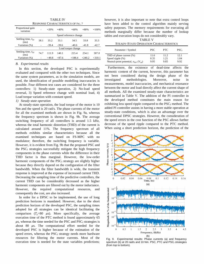
TABLE IV

RESPONSE CHARACTERISTICS OF FIG. 7

Proportional gain variation

- +20% +40%

+60% +80% +100%

Speed reference change

Settling time, 𝑡𝑆𝑆

(ms) 58.1 35.2 35.1

34.5 33.8 33.3

Variation (%) - -39.4 -39.6 -40.6 -41.8 -42.7

Load torque change

Settling time, 𝑡𝑆𝑆

(ms) 74.7 111.9 140.1

215.4 254.1 307.0

Variation (%) - +49.8 +87.6 +188.4 +240.2 +310.1

B. Experimental results

In this section, the developed PSC is experimentally

evaluated and compared with the other two techniques. Since

the same system parameters, as in the simulation models, are

used, the identification of possible modelling inaccuracies is

possible. Four different test cases are considered for the three

controllers: 1) Steady-state operation, 2) No-load speed

reversal, 3) Speed reference change with nominal load, 4)

Load torque variation with constant speed.

1) Steady state operation

At steady-state operation, the load torque of the motor is 10

Nm and the speed is 20 rad/s. The phase currents of the motor

for all the examined methods are shown in Fig. 9a, whereas

the frequency spectrum is shown in Fig. 9b. The average

switching frequency of all controllers is around 1.5 kHz,

whereas the total harmonic distortion (THD) of the current is

calculated around 11%. The frequency spectrum of all

methods exhibits similar characteristics because all the

examined techniques are based on FS-MPC with no

modulator; therefore, the switching frequency is variable.

However, it is evident from Fig. 9b that the proposed PSC and

the PSCf strategies successfully mitigate the high frequency

components in the phase currents while the difference in their

THD factor is thus marginal. However, the low-order

harmonic components of the PSCf strategy are slightly higher

because they directly depend on the configuration of the filter

bandwidth. When the filter bandwidth is wide, the transient

response is improved at the expense of increased current THD.

Decreasing the sampling time of the predictive controllers, the

current THD can be considerably decreased as the higher

harmonic components are filtered out by the motor inductance.

However, the required computational resources, and

consequently the cost, are also increased.

In order for a DPSC to be implemented, the use of long

prediction horizons is mandated. However, due to the short

prediction horizon of the developed PSC, the sampling times

adopted for all strategies can be identical facilitating the

comparison (𝑇𝑠=80 𝜇s). More specifically, the average

execution time of the PTC method is found approximately 65

𝜇s, whereas the time needed for the PSC and PSCf strategies is

about 80 𝜇s. The computational effort needed for the

developed PSC is higher because of the estimation of the

speed errors, whereas the PSCf strategy needs more hardware

resources for filtering the motor currents. Most of the

execution time is needed for the state variables predictions;

however, it is also important to note that extra control loops

have been added to the control algorithm mainly serving

safety purposes. The memory requirements for executing all

methods marginally differ because the number of lookup

tables and execution loops do not considerably vary.

TABLE V

STEADY-STATE OPERATION CHARACTERISTICS

Parameter / Symbol PSC PTC PSCf

THD of phase current (%) 11.6 11.2 12.1 Speed ripple (%) 0.35 1.21 1.04

Neutral-point potential, 𝑣𝑁𝑃 (Vpp) 9.95 9.85 9.92

Furthermore, the existence of dead-time affects the

harmonic content of the current, however, this parameter has

not been considered during the design phase of the

investigated methodologies. Moreover, noise in

measurements, model inaccuracies, and mechanical resonance

between the motor and load directly affect the current shape of

all methods. All the examined steady-state characteristics are

summarized in Table V. The addition of the PI controller in

the developed method constitutes the main reason for

exhibiting less speed ripple compared to the PSCf method. The

added PI controller assists in having a more stable operation at

steady-state conditions, which is also an advantage over the

conventional DPSC strategies. However, the consideration of

the speed errors in the cost function of the PSC allows further

decrease of the speed ripple compared to the PTC method.

When using a short prediction horizon, the prediction of the

(a)

(b)

Fig. 9. Experimental results: Phase currents (a) and frequency spectrum (b) at 20 rad/s and 10 Nm. PSC, PTC and PSCf strategies (from top to bottom).

motor speed is not very accurate, but the consideration of the

speed errors assists in reducing the speed ripple because

switching combinations that cause large steps in the speed are

not considered. The speed ripple in the case of PSC is kept

low, but the mitigation of the high-frequency components is

not as effective as when using the PTC method. This can be

evidenced by the higher current THD of the PSC method. If

regulating the weights, such that both strategies exhibit the

same THD, then the speed ripple of the PSC method is

expected to increase. Furthermore, all methods manage to

keep the voltages of the DC-link capacitors well balanced and

satisfy the inverter specification since the voltage ripple is less

than 20 Vpp. However, the neutral-point potential can be

further reduced by increasing the respective weighting

coefficient, 𝜆𝑁𝑃. Finally, the proposed PSC method benefits

from the consideration of the speed dynamics thus exhibits the

lowest speed ripple compared to the other methods.

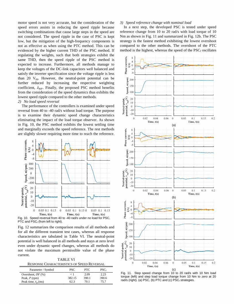
2) No load speed reversal

The performance of the controllers is examined under speed

reversal from 40 to -40 rad/s without load torque. The purpose

is to examine their dynamic speed change characteristics

eliminating the impact of the load torque observer. As shown

in Fig. 10, the PSC method exhibits the lowest settling time

and marginally exceeds the speed reference. The rest methods

are slightly slower requiring more time to reach the reference.

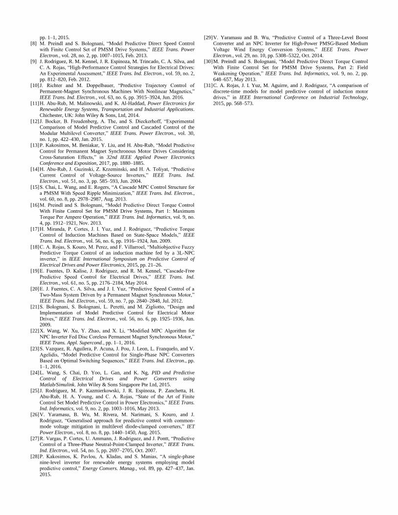
Fig. 12 summarizes the comparison results of all methods and

for all the different transient test cases, whereas all response

characteristics are tabulated in Table VI. The neutral-point

potential is well balanced in all methods and stays at zero level

even under dynamic speed changes, whereas all methods do

not violate the maximum permissible value of the phase

current.

TABLE VI

RESPONSE CHARACTERISTICS OF SPEED REVERSAL

Parameter / Symbol PSC PTC PSCf

Overshoot, 𝑂𝑉 (%) < 1 2.09 2.23

Peak, 𝑃 (rpm) 382.15 390.1 390.6

Peak time, 𝑡𝑝 (ms) 62.3 70.1 75.7

3) Speed reference change with nominal load

In a next step, the developed PSC is tested under speed

reference change from 10 to 20 rad/s with load torque of 10

Nm as shown in Fig. 11 and summarized in Fig. 12b. The PSC

strategy is the fastest method exhibiting the lowest overshoot

compared to the other methods. The overshoot of the PTC

method is the highest, whereas the speed of the PSCf oscillates

Fig. 10. Speed reversal from 40 to -40 rad/s under no load for PSC, PTC and PSCf (from left to right).

(a)

(b)

(c)

Fig. 11. Step speed change from 10 to 20 rad/s with 10 Nm load torque (left) and step load torque change from 10 Nm to zero at 20 rad/s (right). (a) PSC, (b) PTC and (c) PSCf strategies.

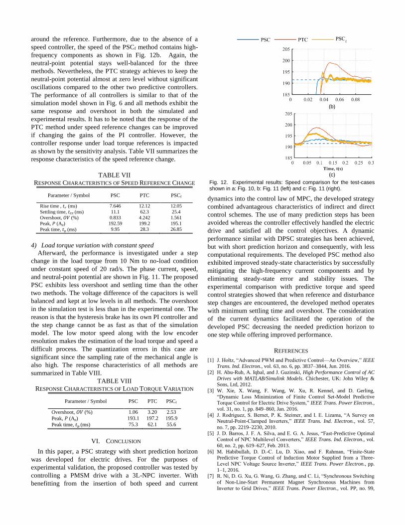
around the reference. Furthermore, due to the absence of a

speed controller, the speed of the PSCf method contains high-

frequency components as shown in Fig. 12b. Again, the

neutral-point potential stays well-balanced for the three

methods. Nevertheless, the PTC strategy achieves to keep the

neutral-point potential almost at zero level without significant

oscillations compared to the other two predictive controllers.

The performance of all controllers is similar to that of the

simulation model shown in Fig. 6 and all methods exhibit the

same response and overshoot in both the simulated and

experimental results. It has to be noted that the response of the

PTC method under speed reference changes can be improved

if changing the gains of the PI controller. However, the

controller response under load torque references is impacted

as shown by the sensitivity analysis. Table VII summarizes the

response characteristics of the speed reference change.

TABLE VII

RESPONSE CHARACTERISTICS OF SPEED REFERENCE CHANGE

Parameter / Symbol PSC PTC PSCf

Rise time , 𝑡𝑟 (ms) 7.646 12.12 12.05

Settling time, 𝑡𝑆𝑆 (ms) 11.1 62.3 25.4

Overshoot, 𝑂𝑉 (%) 0.833 4.242 1.561

Peak, 𝑃 (Ap) 192.59 199.2 195.1

Peak time, 𝑡𝑝 (ms) 9.95 28.3 26.85

4) Load torque variation with constant speed

Afterward, the performance is investigated under a step

change in the load torque from 10 Nm to no-load condition

under constant speed of 20 rad/s. The phase current, speed,

and neutral-point potential are shown in Fig. 11. The proposed

PSC exhibits less overshoot and settling time than the other

two methods. The voltage difference of the capacitors is well

balanced and kept at low levels in all methods. The overshoot

in the simulation test is less than in the experimental one. The

reason is that the hysteresis brake has its own PI controller and

the step change cannot be as fast as that of the simulation

model. The low motor speed along with the low encoder

resolution makes the estimation of the load torque and speed a

difficult process. The quantization errors in this case are

significant since the sampling rate of the mechanical angle is

also high. The response characteristics of all methods are

summarized in Table VIII.

TABLE VIII

RESPONSE CHARACTERISTICS OF LOAD TORQUE VARIATION

Parameter / Symbol PSC PTC PSCf

Overshoot, 𝑂𝑉 (%) 1.06 3.20 2.53

Peak, 𝑃 (Ap) 193.1 197.2 195.9

Peak time, 𝑡𝑝 (ms) 75.3 62.1 55.6

VI. CONCLUSION

In this paper, a PSC strategy with short prediction horizon

was developed for electric drives. For the purposes of

experimental validation, the proposed controller was tested by

controlling a PMSM drive with a 3L-NPC inverter. With

benefitting from the insertion of both speed and current

dynamics into the control law of MPC, the developed strategy

combined advantageous characteristics of indirect and direct

control schemes. The use of many prediction steps has been

avoided whereas the controller effectively handled the electric

drive and satisfied all the control objectives. A dynamic

performance similar with DPSC strategies has been achieved,

but with short prediction horizon and consequently, with less

computational requirements. The developed PSC method also

exhibited improved steady-state characteristics by successfully

mitigating the high-frequency current components and by

eliminating steady-state error and stability issues. The

experimental comparison with predictive torque and speed

control strategies showed that when reference and disturbance

step changes are encountered, the developed method operates

with minimum settling time and overshoot. The consideration

of the current dynamics facilitated the operation of the

developed PSC decreasing the needed prediction horizon to

one step while offering improved performance.

REFERENCES

[1] J. Holtz, “Advanced PWM and Predictive Control—An Overview,” IEEE Trans. Ind. Electron., vol. 63, no. 6, pp. 3837–3844, Jun. 2016.

[2] H. Abu-Rub, A. Iqbal, and J. Guzinski, High Performance Control of AC

Drives with MATLAB/Simulink Models. Chichester, UK: John Wiley & Sons, Ltd, 2012.

[3] W. Xie, X. Wang, F. Wang, W. Xu, R. Kennel, and D. Gerling,

“Dynamic Loss Minimization of Finite Control Set-Model Predictive Torque Control for Electric Drive System,” IEEE Trans. Power Electron.,

vol. 31, no. 1, pp. 849–860, Jan. 2016.

[4] J. Rodriguez, S. Bernet, P. K. Steimer, and I. E. Lizama, “A Survey on Neutral-Point-Clamped Inverters,” IEEE Trans. Ind. Electron., vol. 57,

no. 7, pp. 2219–2230, 2010.

[5] J. D. Barros, J. F. A. Silva, and E. G. A. Jesus, “Fast-Predictive Optimal Control of NPC Multilevel Converters,” IEEE Trans. Ind. Electron., vol.

60, no. 2, pp. 619–627, Feb. 2013.

[6] M. Habibullah, D. D.-C. Lu, D. Xiao, and F. Rahman, “Finite-State Predictive Torque Control of Induction Motor Supplied from a Three-

Level NPC Voltage Source Inverter,” IEEE Trans. Power Electron., pp.

1–1, 2016. [7] R. Ni, D. G. Xu, G. Wang, G. Zhang, and C. Li, “Synchronous Switching

of Non-Line-Start Permanent Magnet Synchronous Machines from

Inverter to Grid Drives,” IEEE Trans. Power Electron., vol. PP, no. 99,

(b)

(c)

Fig. 12. Experimental results: Speed comparison for the test-cases shown in a: Fig. 10, b: Fig. 11 (left) and c: Fig. 11 (right).

pp. 1–1, 2015.

[8] M. Preindl and S. Bolognani, “Model Predictive Direct Speed Control

with Finite Control Set of PMSM Drive Systems,” IEEE Trans. Power

Electron., vol. 28, no. 2, pp. 1007–1015, Feb. 2013. [9] J. Rodriguez, R. M. Kennel, J. R. Espinoza, M. Trincado, C. A. Silva, and

C. A. Rojas, “High-Performance Control Strategies for Electrical Drives:

An Experimental Assessment,” IEEE Trans. Ind. Electron., vol. 59, no. 2, pp. 812–820, Feb. 2012.

[10] J. Richter and M. Doppelbauer, “Predictive Trajectory Control of

Permanent-Magnet Synchronous Machines With Nonlinear Magnetics,” IEEE Trans. Ind. Electron., vol. 63, no. 6, pp. 3915–3924, Jun. 2016.

[11] H. Abu-Rub, M. Malinowski, and K. Al-Haddad, Power Electronics for Renewable Energy Systems, Transportation and Industrial Applications.

Chichester, UK: John Wiley & Sons, Ltd, 2014.

[12] J. Bocker, B. Freudenberg, A. The, and S. Dieckerhoff, “Experimental Comparison of Model Predictive Control and Cascaded Control of the

Modular Multilevel Converter,” IEEE Trans. Power Electron., vol. 30,

no. 1, pp. 422–430, Jan. 2015. [13] P. Kakosimos, M. Beniakar, Y. Liu, and H. Abu-Rub, “Model Predictive

Control for Permanent Magnet Synchronous Motor Drives Considering

Cross-Saturation Effects,” in 32nd IEEE Applied Power Electronics

Conference and Exposition, 2017, pp. 1880–1885.

[14] H. Abu-Rub, J. Guzinski, Z. Krzeminski, and H. A. Toliyat, “Predictive

Current Control of Voltage-Source Inverters,” IEEE Trans. Ind. Electron., vol. 51, no. 3, pp. 585–593, Jun. 2004.

[15] S. Chai, L. Wang, and E. Rogers, “A Cascade MPC Control Structure for

a PMSM With Speed Ripple Minimization,” IEEE Trans. Ind. Electron., vol. 60, no. 8, pp. 2978–2987, Aug. 2013.

[16] M. Preindl and S. Bolognani, “Model Predictive Direct Torque Control

With Finite Control Set for PMSM Drive Systems, Part 1: Maximum Torque Per Ampere Operation,” IEEE Trans. Ind. Informatics, vol. 9, no.

4, pp. 1912–1921, Nov. 2013.

[17] H. Miranda, P. Cortes, J. I. Yuz, and J. Rodriguez, “Predictive Torque Control of Induction Machines Based on State-Space Models,” IEEE

Trans. Ind. Electron., vol. 56, no. 6, pp. 1916–1924, Jun. 2009.

[18] C. A. Rojas, S. Kouro, M. Perez, and F. Villarroel, “Multiobjective Fuzzy Predictive Torque Control of an induction machine fed by a 3L-NPC

inverter,” in IEEE International Symposium on Predictive Control of

Electrical Drives and Power Electronics, 2015, pp. 21–26. [19] E. Fuentes, D. Kalise, J. Rodriguez, and R. M. Kennel, “Cascade-Free

Predictive Speed Control for Electrical Drives,” IEEE Trans. Ind.

Electron., vol. 61, no. 5, pp. 2176–2184, May 2014. [20] E. J. Fuentes, C. A. Silva, and J. I. Yuz, “Predictive Speed Control of a

Two-Mass System Driven by a Permanent Magnet Synchronous Motor,”

IEEE Trans. Ind. Electron., vol. 59, no. 7, pp. 2840–2848, Jul. 2012. [21] S. Bolognani, S. Bolognani, L. Peretti, and M. Zigliotto, “Design and

Implementation of Model Predictive Control for Electrical Motor

Drives,” IEEE Trans. Ind. Electron., vol. 56, no. 6, pp. 1925–1936, Jun. 2009.

[22] X. Wang, W. Xu, Y. Zhao, and X. Li, “Modified MPC Algorithm for

NPC Inverter Fed Disc Coreless Permanent Magnet Synchronous Motor,” IEEE Trans. Appl. Supercond., pp. 1–1, 2016.

[23] S. Vazquez, R. Aguilera, P. Acuna, J. Pou, J. Leon, L. Franquelo, and V.

Agelidis, “Model Predictive Control for Single-Phase NPC Converters Based on Optimal Switching Sequences,” IEEE Trans. Ind. Electron., pp.

1–1, 2016.

[24] L. Wang, S. Chai, D. Yoo, L. Gan, and K. Ng, PID and Predictive Control of Electrical Drives and Power Converters using

Matlab/Simulink. John Wiley & Sons Singapore Pte Ltd, 2015.

[25] J. Rodriguez, M. P. Kazmierkowski, J. R. Espinoza, P. Zanchetta, H. Abu-Rub, H. A. Young, and C. A. Rojas, “State of the Art of Finite

Control Set Model Predictive Control in Power Electronics,” IEEE Trans. Ind. Informatics, vol. 9, no. 2, pp. 1003–1016, May 2013.

[26] V. Yaramasu, B. Wu, M. Rivera, M. Narimani, S. Kouro, and J.

Rodriguez, “Generalised approach for predictive control with common-mode voltage mitigation in multilevel diode-clamped converters,” IET

Power Electron., vol. 8, no. 8, pp. 1440–1450, Aug. 2015.

[27] R. Vargas, P. Cortes, U. Ammann, J. Rodriguez, and J. Pontt, “Predictive Control of a Three-Phase Neutral-Point-Clamped Inverter,” IEEE Trans.

Ind. Electron., vol. 54, no. 5, pp. 2697–2705, Oct. 2007.

[28] P. Kakosimos, K. Pavlou, A. Kladas, and S. Manias, “A single-phase nine-level inverter for renewable energy systems employing model

predictive control,” Energy Convers. Manag., vol. 89, pp. 427–437, Jan.

2015.

[29] V. Yaramasu and B. Wu, “Predictive Control of a Three-Level Boost Converter and an NPC Inverter for High-Power PMSG-Based Medium

Voltage Wind Energy Conversion Systems,” IEEE Trans. Power

Electron., vol. 29, no. 10, pp. 5308–5322, Oct. 2014. [30] M. Preindl and S. Bolognani, “Model Predictive Direct Torque Control

With Finite Control Set for PMSM Drive Systems, Part 2: Field

Weakening Operation,” IEEE Trans. Ind. Informatics, vol. 9, no. 2, pp. 648–657, May 2013.

[31] C. A. Rojas, J. I. Yuz, M. Aguirre, and J. Rodriguez, “A comparison of

discrete-time models for model predictive control of induction motor drives,” in IEEE International Conference on Industrial Technology,

2015, pp. 568–573.