predictive analytics for transportation in a high...
TRANSCRIPT

COLLABORATE. INNOVATE. EDUCATE.
Predictive Analytics for
Transportation Planning and
Operations in a World of Big Data
Chandra R. Bhat
The University of Texas at Austin
Acknowledgments: D-STOP, TxDOT (Jianming Ma+), NCTCOG, Humboldt Award, Dr. Ram Pendyala, Dr. Kostas Goulias, Dr. Abdul Pinjari, all my graduate/undergraduate students

COLLABORATE. INNOVATE. EDUCATE.
World of high dimensional
heterogeneous data
Providing accurate traffic information is becoming a major challenge.
Cameras, GPS, cell phone tracking, and probe vehicles are used to supplement the information provided by conventional measurement systems.
Methodologies to combine and aggregate high dimensional heterogeneous data are needed

COLLABORATE. INNOVATE. EDUCATE.
Connected/Automated Vehicles
(CAVs) and big data
The driverless car of the near future is part of a gigantic data-collection engine.
Vehicles have embedded computers, GPS receivers, short-range wireless network interfaces, in-car sensors, cameras, and internet.
Vehicles interact with Roadside wireless sensor networks, passenger’s wireless devices, and other cars.

COLLABORATE. INNOVATE. EDUCATE.
Data required to keep a self-driving
car safely on the road
Highly detailed maps information: Shape and elevation of roadways, lane lines, intersections, crosswalks, speed limits, and traffic signals.
Position, speed and intentions of other vehicles and pedestrians.
Position, speed and intentions of unexpected obstacles, such as, jaywalking pedestrians, cars lunching out of hidden driveways, a stop sign held up by a crossing guard, and cyclist making gestures.

What can be inferred from CAVs and
smartphones data
• Where people drive,
• when people drive,
• what route people take,
• where people stop,
• what people put in their car,
• why, how and when people take decisions on the fly and change their activity plan route, and
• detailed crashes data (speed, position, and intention at the moment of the accident).

COLLABORATE. INNOVATE. EDUCATE.
Self-Driving Vehicle (e.g., Google) Connected Vehicle
AI located within the vehicle AI wirelessly connected to an external communications network
“Outward-facing” in that sensors blast outward from the vehicle to collect information without receiving data inward from other sources
“Inward-facing” with the vehicle receiving external environment information through wireless connectivity, and operational commands from an external entity
AI used to make autonomous decisions on what is best for the individual driver
Used in cooperation with other pieces of information to make decisions on what is “best” from a system optimal standpoint
AI not shared with other entities beyond the vehicle
AI shared across multiple vehicles
A more “Capitalistic” set-up A more “Socialistic” set-up
Two Types of Technology
COLLABORATE. INNOVATE. EDUCATE.
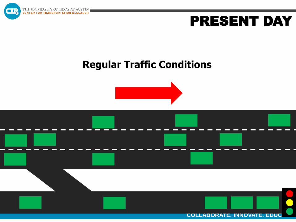
Regular Traffic Conditions
PRESENT DAY

COLLABORATE. INNOVATE. EDUCATE.
Icy Patch
PRESENT DAY

COLLABORATE. INNOVATE. EDUCATE.
Incident
PRESENT DAY

COLLABORATE. INNOVATE. EDUCATE.
Lane blocking, traffic slow down
PRESENT DAY
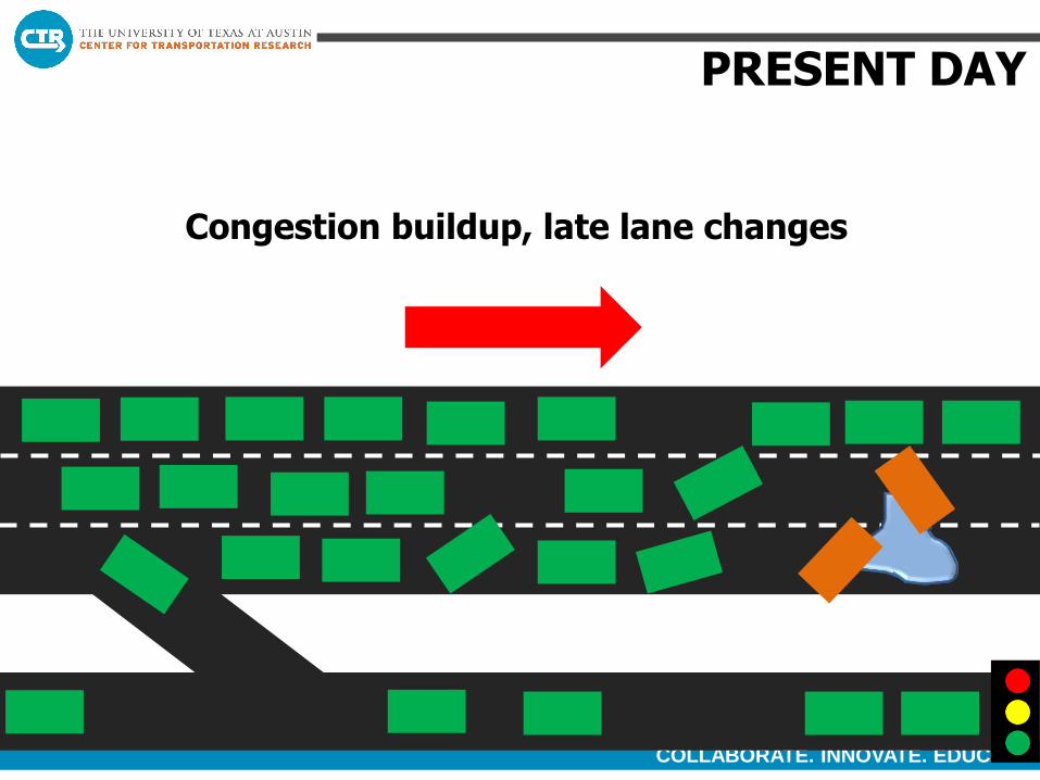
COLLABORATE. INNOVATE. EDUCATE.
Congestion buildup, late lane changes
PRESENT DAY

COLLABORATE. INNOVATE. EDUCATE.
Congestion propagation to frontage, ramp backed up
PRESENT DAY

COLLABORATE. INNOVATE. EDUCATE.
Regular Traffic Conditions
V2V

COLLABORATE. INNOVATE. EDUCATE.
Icy Patch
V2V

COLLABORATE. INNOVATE. EDUCATE.
Incident: Information propagation
V2V

COLLABORATE. INNOVATE. EDUCATE.
Preemptive lane changing, freeway exit
V2V

COLLABORATE. INNOVATE. EDUCATE.
Re-optimization of signal timing, upstream detours
INCIDENT AHEAD TAKE
DETOUR
V2I

COLLABORATE. INNOVATE. EDUCATE.
Regular Traffic Conditions
AUTONOMOUS

COLLABORATE. INNOVATE. EDUCATE.
Icy Patch
AUTONOMOUS

COLLABORATE. INNOVATE. EDUCATE.
Avoidance of icy patch, no incident
AUTONOMOUS
COLLABORATE. INNOVATE. EDUCATE.
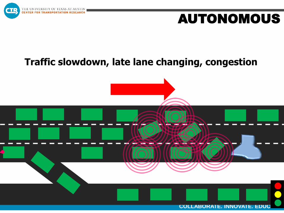
Traffic slowdown, late lane changing, congestion
AUTONOMOUS

COLLABORATE. INNOVATE. EDUCATE.
Icy Patch
AUTONOMOUS + V2X

COLLABORATE. INNOVATE. EDUCATE.
Avoidance of icy patch, no incident
AUTONOMOUS + V2X

COLLABORATE. INNOVATE. EDUCATE.
Information propagation, preemptive lane changing, freeway exit
AUTONOMOUS + V2V

COLLABORATE. INNOVATE. EDUCATE.
Re-optimization of signal timing, upstream detours
INCIDENT AHEAD TAKE
DETOUR
AUTONOMOUS + V2I

COLLABORATE. INNOVATE. EDUCATE.
Traffic safety is an urgent necessity!
5.7 million crashes in the US in 2013* Enormous cost to society
2,310,000
Injuries in the US in 2013*
232,041 (10%)
Injuries in TX**
*: NHTSA, 2014
**: TxDOT, 2014
Property damage Productivity loss Injury Death
Cost almost $1 trillion!!!
26
32,719
Deaths in the US in 2013*
3.382 (10%)
Deaths in TX**
81% of all annual crashes can potentially
be addressed by vehicle-to-vehicle and
vehicle-to-infrastructure
systems***
***: USDOT, 2015

COLLABORATE. INNOVATE. EDUCATE.
Multidisciplinary approach to improve Collision
Warning/ Avoidance Systems (CW/CA)
CAR-STOP
TRANSPORTATION
WIRELESS MACHINE
LEARNING
Communication
and radar
technologies
Distributed
decision
making
Transportation aspects
27

COLLABORATE. INNOVATE. EDUCATE.
Proposed Approach
Prior Info Real-time
info Prediction for CW/CA
IMPROVED
SAFETY
Exploit prior info o Driver´s behavior o Typical traffic condition
Joint radar and communications o Waveform / hardware / antenna design o Security needed to prevent spoofing
Collision warning/avoidance algorithms o Smart combination of information o Distributed decision making
SAFE
28

COLLABORATE. INNOVATE. EDUCATE.
Benefits of sharing raw sensor data
29
Live streaming of lead vehicle’s front sensor info
Front sensors
Exchanging raw sensor data makes overtaking safer
Rural roadway overtaking scenario

COLLABORATE. INNOVATE. EDUCATE.
Improving safety for 3 types of traffic
configurations
30
Urban intersections [1]
Rural roads [2]
High density of pedestrians and bicyclists [3]
Sources: [1]Google Maps – City of Austin; [2] atzonline.com; [3] dailytexanonline.com

COLLABORATE. INNOVATE. EDUCATE.
Real-time Fusion
31
Radar Detection
On-vehicle Sensors
V2V Messages

COLLABORATE. INNOVATE. EDUCATE.
Exploiting additional sources of
information
32
Radar Detection
On-vehicle Sensors
V2V Messages
Road Topology
Previous Behavior
Extra V2V Messaging

COLLABORATE. INNOVATE. EDUCATE.
Driver A
Driver B
Driver C
Faster left turn
Slower braking
Personal Motion
Predictor …
Driver history
Personal Motion
Predictor
Predicted better with driver history
Storing and making use of driver history
Months 1-9
33

COLLABORATE. INNOVATE. EDUCATE.
o Maps provide vital information on expected future motion
o Improve map-based prediction algorithm for CW/CA
OpenStreetMap[1]
Google Maps API[2]
Available road maps
Motion Predictor
[1] www.openstreetmap.org [2] developers.google.com/maps
Work Package 1.3.2
Months 4-14
Acquiring and using location context
34
COLLABORATE. INNOVATE. EDUCATE.
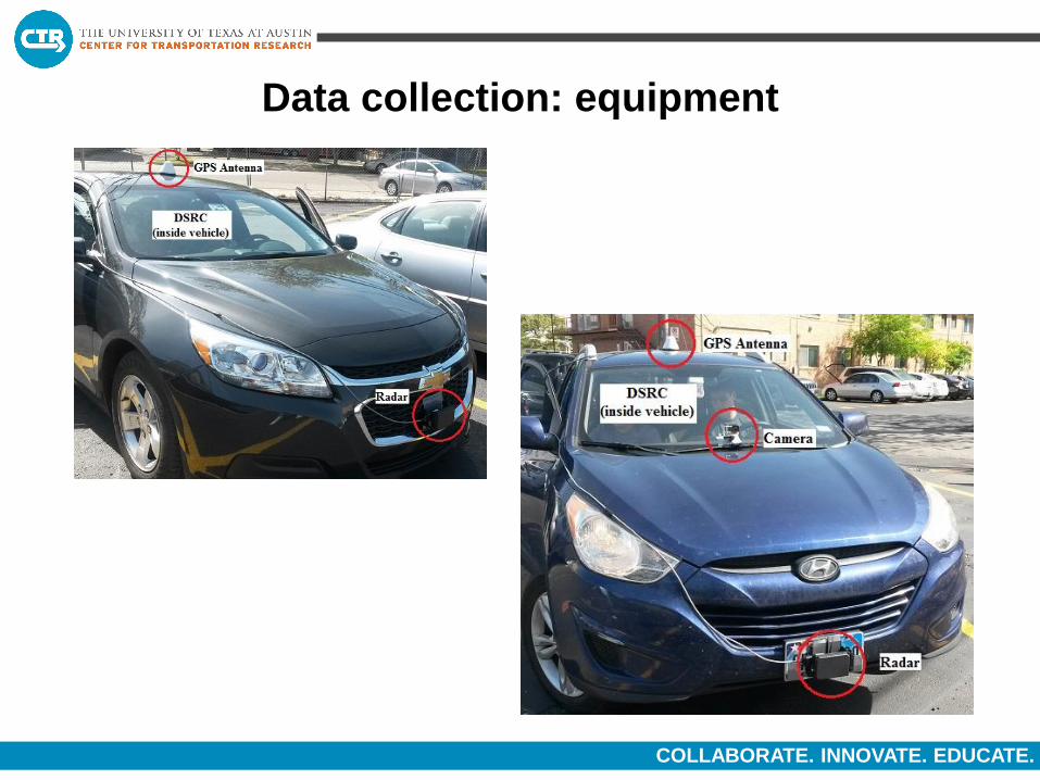
Data collection: equipment

COLLABORATE. INNOVATE. EDUCATE.
Performance of joint system: blind intersection
scenario
36

COLLABORATE. INNOVATE. EDUCATE.
Performance of joint system: position accuracy
37

COLLABORATE. INNOVATE. EDUCATE.
Performance of joint system: pedestrians and
bicyclists
38

•
•
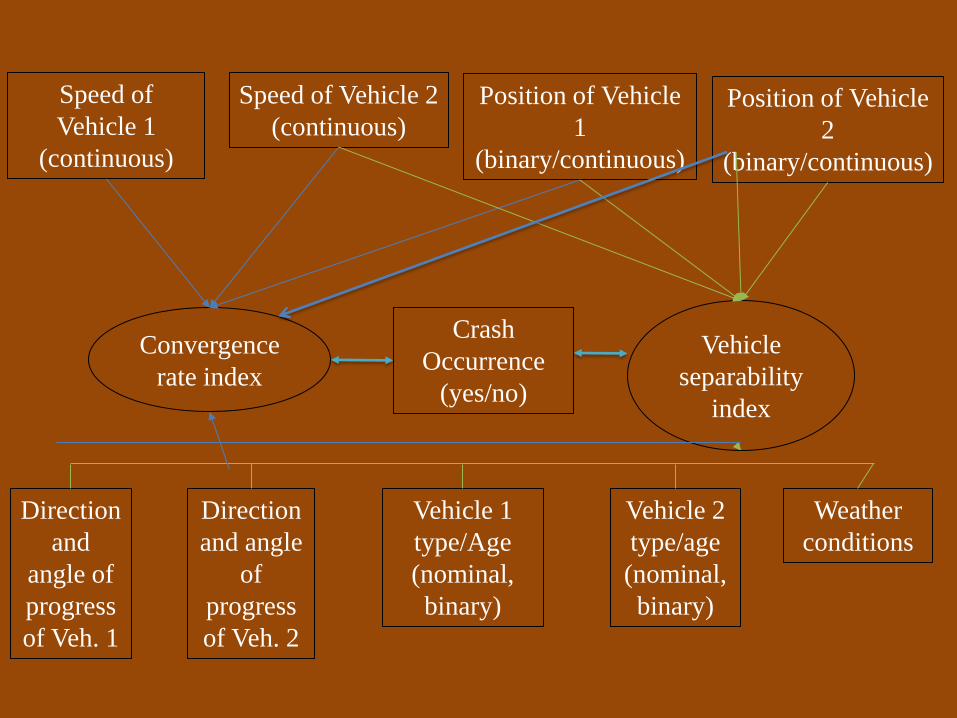
Position of Vehicle
1
(binary/continuous)
Speed of Vehicle 2
(continuous) Position of Vehicle
2
(binary/continuous)
Speed of
Vehicle 1
(continuous)
Direction
and
angle of
progress
of Veh. 1
Direction
and angle
of
progress
of Veh. 2
Vehicle 1
type/Age
(nominal,
binary)
Vehicle 2
type/age
(nominal,
binary)
Weather
conditions
Convergence
rate index
Vehicle
separability
index
Crash
Occurrence
(yes/no)

Data Science
• Not enough humans to process
• Machine learning, visualization, and advanced computation techniques
• Statistics, social sciences, and domain knowledge
• High-dimensional heterogeneous data

COLLABORATE. INNOVATE. EDUCATE.
Infrastructure Needs/Planning
Driven By…
Complex activity-travel patterns
Growth in long distance travel demand
Limited availability of land to dedicate to infrastructure
Budget/fiscal constraints
Energy and environmental concerns
Information/ communication technologies (ICT) and mobile platform advances
Autonomous vehicles leverage technology to increase flow without the need to expand capacity
COLLABORATE. INNOVATE. EDUCATE.
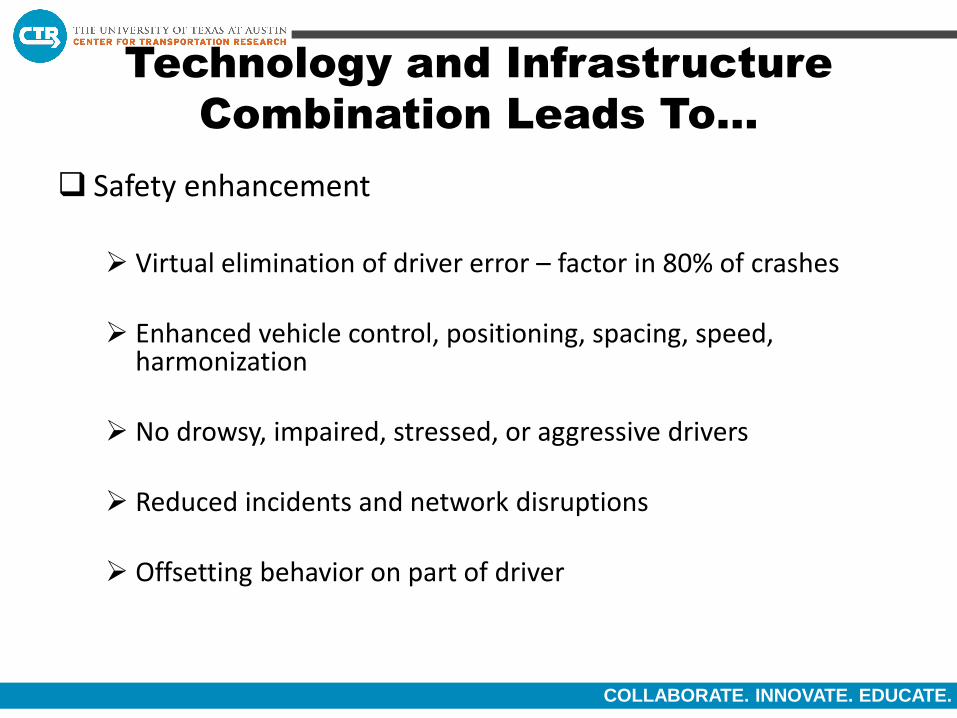
Technology and Infrastructure
Combination Leads To…
Safety enhancement Virtual elimination of driver error – factor in 80% of crashes
Enhanced vehicle control, positioning, spacing, speed,
harmonization
No drowsy, impaired, stressed, or aggressive drivers
Reduced incidents and network disruptions
Offsetting behavior on part of driver

COLLABORATE. INNOVATE. EDUCATE.
Capacity enhancement Platooning reduces headways and improves flow at transitions
Vehicle positioning (lateral control) allows reduced lane widths and
utilization of shoulders; accurate mapping critical
Optimized route choice
Energy and environmental benefits
Increased fuel efficiency and reduced pollutant emissions
Clean fuel vehicles
Car-sharing

COLLABORATE. INNOVATE. EDUCATE.
BUT LET’S NOT FORGET
TRAVELER BEHAVIOR
ISSUES!

COLLABORATE. INNOVATE. EDUCATE.
Impacts on Land-Use Patterns
Live and work farther away Use travel time productively Access more desirable and higher paying job Attend better school/college
Visit destinations farther away
Access more desirable destinations for various activities
Reduced impact of distances and time on activity participation
Influence on developers
Sprawled cities? Impacts on community/regional planning and
urban design

COLLABORATE. INNOVATE. EDUCATE.
Impacts on Household Vehicle Fleet
Potential to redefine vehicle ownership No longer own personal vehicles; move toward car sharing enterprise where
rental vehicles come to traveler
More efficient vehicle ownership and sharing scheme may reduce the
need for additional infrastructure Reduced demand for parking
Desire to work and be productive in vehicle
More use of personal vehicle for long distance travel
Purchase large multi-purpose vehicle with amenities to work and play in
vehicle

COLLABORATE. INNOVATE. EDUCATE.

COLLABORATE. INNOVATE. EDUCATE.
Impacts on Mode Choice
Automated vehicles combine the advantages of public transportation with that of traditional private vehicles
Catching up on news Texting friends Reading novels
Flexibility Comfort Convenience
What will happen to public transportation?
Also automated vehicles may result in lesser walking and bicycling shares
Time less of a consideration So, will Cost be the main policy tool to influence behavior?

COLLABORATE. INNOVATE. EDUCATE.
Impacts on Mode Choice
Driving personal vehicle more convenient and safe
Traditional transit captive market segments now able to use auto (e.g., elderly, disabled)
Reduced reliance/usage of public transit?
However, autonomous vehicles may present an opportunity for public transit and car sharing Lower cost of operation (driverless) and can cut out low volume routes
More personalized and reliable service - smaller vehicles providing demand-responsive transit
service
No parking needed – kiss-and-ride; no vehicles “sitting” around
20-80% of urban land area can be reclaimed
Chaining may not discourage transit use

COLLABORATE. INNOVATE. EDUCATE.
Activity Chaining Issues
Drive Alone
Drive Alone Drive Alone
Shopping
Home Work
Very Good Transit Service

COLLABORATE. INNOVATE. EDUCATE.
Impacts on Long Distance Travel
Less incentive to use public transportation?
Should we even be investing in high capital high-speed rail systems?
Individuals can travel and sleep in driverless cars
Individuals may travel mostly in the night
Speed difference?

COLLABORATE. INNOVATE. EDUCATE.
Impacts on Commercial Vehicle
Operations
Enhanced efficiency of commercial vehicle operations
Driverless vehicles operating during off-peak and night hours reducing congestion
Reduced need for infrastructure

COLLABORATE. INNOVATE. EDUCATE.
Mixed Vehicle Operations
Uncertainty in penetration rates of driverless cars
Considerable amount of time of both driverless and traditional car operation
When will we see full adoption of autonomous? Depends on regulatory policies
Need infrastructure planning to support both, with intelligent/dedicated infrastructure for driverless
COLLABORATE. INNOVATE. EDUCATE.
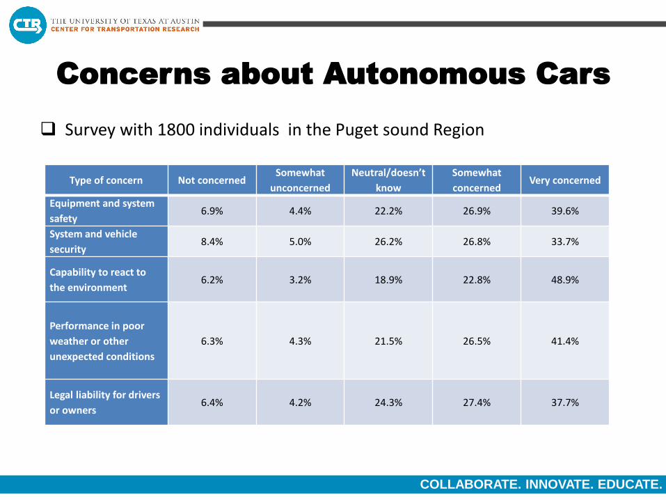
Concerns about Autonomous Cars
Survey with 1800 individuals in the Puget sound Region
Type of concern Not concerned Somewhat
unconcerned
Neutral/doesn’t
know
Somewhat
concerned Very concerned
Equipment and system
safety 6.9% 4.4% 22.2% 26.9% 39.6%
System and vehicle
security 8.4% 5.0% 26.2% 26.8% 33.7%
Capability to react to
the environment 6.2% 3.2% 18.9% 22.8% 48.9%
Performance in poor
weather or other
unexpected conditions
6.3% 4.3% 21.5% 26.5% 41.4%
Legal liability for drivers
or owners 6.4% 4.2% 24.3% 27.4% 37.7%

COLLABORATE. INNOVATE. EDUCATE.

DOMAIN KNOWLEDGE IN THE CONTEXT
OF TRAVEL DEMAND MODELING

Exogenous Variable Vector X
Model
• Conceptual/Theoretical/ Methods/Tools and Techniques
• Specification and Definition of Alternatives
Activity-Based Model (ABM) Trip-based Model (TBM)
Outputs

• ABM should…
Capture the central role of activities, time, and space in a continuum
Explicitly recognize constraints and interactions
Represent simultaneity in behavioral choice processes
Account for heterogeneity in behavioral decision hierarchies
Incorporate feedback processes to facilitate integration with land use and network models
• SimAGENT does it all …

SIMAGENT (SIMULATOR OF ACTIVITIES,
GREENHOUSE GAS EMISSIONS, ENERGY,
NETWORKS, AND TRAVEL)

HIGH DIMENSIONAL HETEROGENEOUS
DATA

Why joint modeling of data is important?
• Borrows information on other outcomes
• Able to answer intrinsically multivariate questions, such as the effect of a covariate on a multidimensional outcome
• Obviates the need for multiple tests and facilitates global tests, offering superior testing power and better control of Type 1 error rates
• If some endogenous outcomes are used to explain other endogenous outcomes, and if the outcomes are not modeled jointly, the result can be inconsistent estimation of the effects of one endogenous outcome on another.
• Problem? Mixed data, high-dimensional data

Way-Out
• The new Generalized Heterogeneous Data Model (GHDM).
• Correlation across various dimensions (of the dependent variables) are captured using latent constructs.
• Reduces the size of error covariance elements.
• Accommodates all four types of data (dependent variables).
• Dimension of integration is independent of number of latent constructs.
• Bhat’s Maximum Approximate Composite Marginal Likelihood (MACML) estimation approach is used for estimation of GHDM.

• Integrated modeling = Acknowledging the joint nature of decision-making relevant to inter-related outcomes.
• Jointness may arise because of the impact (on the multiple
choice outcomes) of
common underlying exogenous observed variables
common underlying exogenous unobserved variables
combination of both

• Example: Consider residential location, auto-ownership, and activity time-use.
• Households with low income earnings may…
choose to (or are constrained to) locate in neighborhoods with high population density,
have low household auto ownership levels, and
spend less time in recreational episodes
• If the elements causing jointness are solely due to observed exogenous factors, then modeling is straightforward.

COLLABORATE. INNOVATE. EDUCATE.
Framework for dwelling unit choice and activity-travel behavior

COLLABORATE. INNOVATE. EDUCATE.
Activity Travel Behavior and Health Indicators

An Example
• New econometric approach for the estimation of joint mixed models that include:
MDC outcome
nominal discrete outcome
count, binary/ordinal outcomes, as well as continuous outcomes
• Specify latent underlying unobserved factors that impact the many outcomes, and generate the jointness among the outcomes
• Reported subjective attitudinal indicators for the latent variables help provide additional information and stability to the model system
• Application: analysis of residential location choice, household auto-ownership choice, as well as time-use choices

• Residential location choice:
nominal discrete choice with four land-use density categories as defined by housing unit density (housing units per square mile) within census blocks
continuous outcome representing average commute distance
• Household auto ownership is a count outcome
• Individual activity time-use by activity type in non-work activities is an MDC outcome
• To our knowledge, this is the first formulation and application of such an integrated model system in the econometric and statistical literature
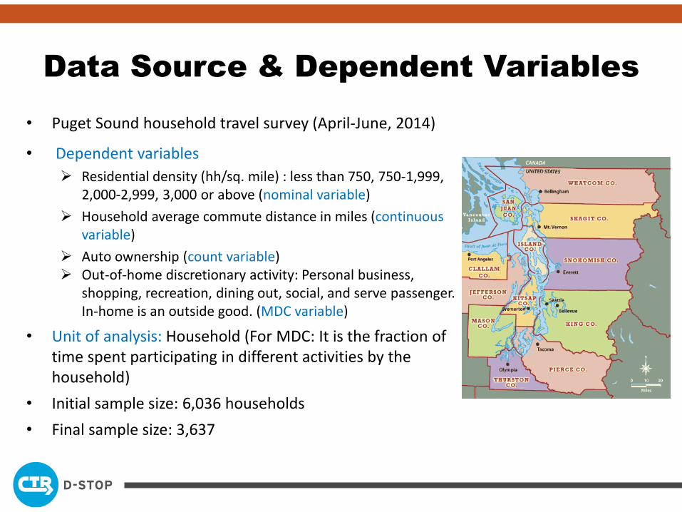
Data Source & Dependent Variables
• Puget Sound household travel survey (April-June, 2014)
• Dependent variables
Residential density (hh/sq. mile) : less than 750, 750-1,999, 2,000-2,999, 3,000 or above (nominal variable)
Household average commute distance in miles (continuous variable)
Auto ownership (count variable) Out-of-home discretionary activity: Personal business,
shopping, recreation, dining out, social, and serve passenger. In-home is an outside good. (MDC variable)
• Unit of analysis: Household (For MDC: It is the fraction of time spent participating in different activities by the household)
• Initial sample size: 6,036 households
• Final sample size: 3,637

Indicator variable: Ordinal variables
Attitudinal Question
Response
Very
Unimportant
1 2 3 4
Very
Important
5
How important when choosing current
home:
Having a walkable neighborhood and
being near to local activities 5.5% 7.6% 11.1% 32.3% 43.5%
Being close to public transit 15.4% 12.0% 17.0% 24.8% 30.8%
Being within a 30-minute commute to
work 6.6% 6.5% 10.0% 24.4% 52.5%
Quality of schools (K-12) 31.2% 7.5% 26.7% 14.6% 20.0%
Having space and separation from
others 9.2% 13.7% 21.8% 34.3% 21.0%
Being close to the highway 12.7% 16.0% 21.4% 38.0% 11.9%

Dependent variable: Count variable
Motorized
Vehicle Count
Frequency
0 1 2 3 4 5 >6
Number 304 1,378 1,354 413 135 36 17
% 8.4 37.8 37.2 11.4 3.7 1.0 0.5
Dependent variable: MNP variable
Residential Density
(households per sq. mile) Number of observations (%)
<750 478 (13.2)
750-2,000 866 (23.8)
2,000-3,000 525 (14.4)
>3,000 1,768 (48.6)

Dependent variable: MDC variable
Activity Participation (%) Mean
fraction
Number of households (% of
total number) spent time…
Only in activity
type
In other
activity types
too
In home (IH) 3,637 (100.0) 0.780 533 (14.7) 3,104 (85.3)
Personal Business 1,607 ( 44.2) 0.202 216 (13.4) 1,391 (86.6)
Shopping 1,664 ( 45.8) 0.060 355 (21.3) 1,309 (78.7)
Recreation 1,011 ( 27.8) 0.131 148 (14.6) 863 (85.4)
Dining Out 1,092 ( 30.0) 0.081 203 (18.6) 889 (81.4)
Social 659 ( 18.1) 0.180 82 (12.4) 557 (87.6)
Serve Passenger 751 ( 20.6) 0.047 26 ( 3.5) 725 (96.5)
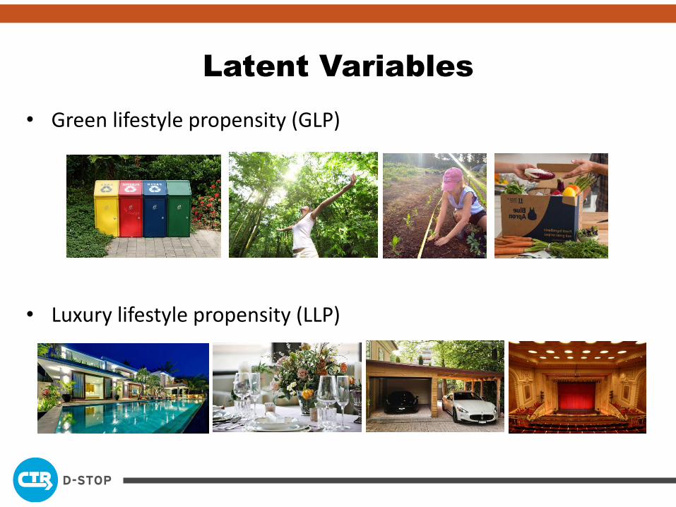
Latent Variables
• Green lifestyle propensity (GLP)
• Luxury lifestyle propensity (LLP)

Indicators
• Green lifestyle propensity (GLP) Average household commute distance (continuous)
Auto ownership (count)
Having a walkable neighborhood (ordinal with five scale)
Being close to public transit (ordinal with five scale)
Being within a 30-minute commute to work (ordinal with five scale)
• Luxury lifestyle propensity (LLP) Auto ownership (count)
Having space and separation from others (ordinal with five scale)
Quality of schools (ordinal with five scale)
Being close to the highway (ordinal with five scale)

Latent Variable Determinants
Green Lifestyle Propensity:
• Lower income households have a higher GLP relative to higher income.
• Households with a high fraction of young adults (less than the age of 34 years) have a higher GLP relative to those with a low fraction of young adults.
• Higher GLP associated with households with a high fraction of women (relative to a low fraction of women) and a high fraction of well-educated individuals in the household (relative to a low fraction of well-educated individuals).

Luxury Lifestyle Propensity:
• LLP increases with household income
• LLP increases with the number of children in the household
• LLP increases with the age of household members
Correlation between GLP and LLP:
Negative correlation (a green lifestyle is associated with conservative consumption of resources, while a luxury lifestyle correlates with extravagant living)

Effect of Latent Constructs
• Households with a GLP disposition
will prefer to reside in high density neighborhoods close to their workplace,
own few or no vehicles,
and engage more in IH activities and OH social and active recreation activities
• Households with an LLP disposition
will be inclined to locate in low to medium density neighborhoods,
own many vehicles,
and potentially be engaged in more OH shopping and dining out activities

Endogenous Effects
• Residential density of the household’s location impacts the household auto ownership level and household activity time use.
Residing in lower (higher) density neighborhoods leads to a higher (lower) auto ownership level and lower (higher) baseline preferences for OH recreational activities, shopping, and dining out.
Time investment in serve passenger activity increases as one moves from the highest density neighborhoods to progressively lower density neighborhoods.
• Commute distance impacts only time use.
Households with longer commute distances spend more time on shopping, recreation, and dining out.

Examining “True” Effects of
Neo-Urbanist Densification Efforts
Variable ATE from GHDM ATE from IHDM
% Difference Attributable to
“True” Effect Self-Selection
Effect Vehicle ownership
-0.143 (0.011) -0.340 (0.021) 42 58
Participation on
Personal business
-0.037 (0.013) -0.041 (0.013) 90 10
Shopping 0.011 (0.004) 0.019 (0.007) 65 35
Recreation 0.134 (0.021) 0.190 (0.014) 71 29
Dining out 0.094 (0.020) 0.119 (0.021) 79 21
Social -0.056 (0.014) -0.078 (0.017) 72 28
Serve Passenger -0.156 (0.033) -0.162 (0.025) 96 4
Table: Treatment Effects Corresponding to Transplanting a Random Household from a Lowest Density Neighborhood (<750 hh/sq. mile) to Highest Density Neighborhood (>3000 hh/sq. mile)
(standard error in parenthesis)
The Bottom Line
Uncertainty, Uncertainty, Uncertainty
More uncertainty implies more need for planning
But planning must recognize the uncertainty (need a change in current thinking and philosophy)


Five Pillars of ABM Design
• Based on sound behavioral theory/paradigm
• Computationally feasible and tractable
– Model estimation
– Model implementation
• Optimal use of available data (present and future)
• ABM should be both an Activity-Based Model and an Agent-Based Model
• Sensitive to policy issues and planning applications of interest

Behavioral Basis of ABM
• Decision hierarchies and choice processes
– A variety of behavioral decision structures possible
– Virtually all models assume a sequential decision structure similar to traditional four-step models for computational convenience
• Considerable evidence of simultaneity in behavioral choice mechanisms
– Several choices made simultaneously as a lifestyle package

Behavioral Basis of ABM
• Examples of simultaneous choice packages
– Residential location, vehicle ownership, mode to pre-planned activities (e.g., work)
– Activity type, activity duration, and activity timing (scheduling)
• Behavioral heterogeneity
– Differences in choice processes across market segments
– Identify market segments both exogenously and endogenously (latent market segments)

Time-Space Interactions
Home Work
Activity 1 (Fixed)
Activity 2 (Fixed) Ti
me
Urban Space
1
v
Home Activity
A
Activity at Location A
Activity 1
Activity 2

Agent Interactions
I have a client meeting today; so I will take the
car
I have to pick up Jane from School and go shopping later; I need the
car.
My meeting is in the morning. I can pick up
Jane from school today. And we can go shopping together in the evening. OK, that sounds
good. I’ll go ahead and take
light rail today to work. See you
later.
Hey, Mom and Dad, don’t forget; you have to drop
me off at Johnny’s house in the
evening today
Don’t worry Jane; we’ll drop you off on the way to the store and pick you up later. Run along now,
you’ll miss the bus.

Definition of an Activity
• Disaggregate activity purpose definition
– Challenge traditional notion of mandatory and discretionary activities/trips
– Movie, ball game, and child’s tennis lesson or soccer game often have spatial and/or temporal fixity
– Characterize activities and trips by level of spatial and temporal fixity/constraints (besides purpose)
– Can be accomplished using concepts of time-space geography
– Automated method to add attributes describing degrees of freedom according to set of spatial/temporal fixity criteria to activity records in data set

Central Role of Time Use
• Notion of time is central to activity-based modeling
– Explicit modeling of activity durations (daily activity time allocation and individual episode duration)
– Treat time as “continuous” and not as “discrete choice” blocks
• Activity engagement is the focus of attention
– Travel patterns are inferred as an outcome of activity participation and time use decisions
– Continuous treatment of time dimension allows explicit consideration of time constraints on human activities
• Reconcile activity durations with network travel durations (feedback
processes)

In Summary
• ABM should…
– Capture the central role of activities, time, and space in a continuum
– Explicitly recognize constraints and interactions
– Represent simultaneity in behavioral choice processes
– Account for heterogeneity in behavioral decision hierarchies
– Incorporate feedback processes to facilitate integration with land use and network models
• SimAGENT does it all …

• Individuals who are intrinsically dynamic with an active lifestyle may….
search for high density neighborhoods that offer high accessibility to activity locations,
own fewer autos, and
invest substantial time in recreational pursuits
• When an unobserved factor affects the multiple outcomes,
Independently modeling
→ inefficient estimation of covariate effects for each outcome
→ inconsistent estimation of the effects of one endogenous outcome on another

CEMDAP
A COMPREHENSIVE ECONOMETRIC
MICROSIMULATOR OF DAILY
ACTIVITY-TRAVEL PATTERNS

CEMDAP – The Core ABM in SimAGENT
Socio-Economic Data
PopGen
CEMSELTS
CEMDAP
• Simulates activity schedule and travel characteristics for each individual of the region
• Core module of SimAGENT
• 52 sub-models.
• Developed by UT Austin

Features of CEMDAP (continued)
• Changes in the activity-travel pattern of one individual in a household may bring about changes in activity-travel patterns of other household members
• MDCEV approach facilitates modeling activity participation at a
household level with joint activity participation incorporated in
a simple fashion
– MDCEV – Multiple Discrete Continuous Extreme Value
econometric choice modeling method
• Includes a model of household vehicle ownership by type and make/model, and primary driver assignment

INNOVATION:
COMPREHENSIVE REPRESENTATION OF
INTRA-HOUSEHOLD INTERACTIONS

Joint Activities and Household Interactions
MDCEV Model
• Most activity based models accommodate activity type choice as a series of models for each individual in the household
• These approaches do not explicitly recognize that activity participation is a collective decision of household members
• MDCEV approach – simple and relatively inexpensive for modeling activity participation at a household level
• SimAGENT now features MDCEV modeling methodology to capture household-level activity participation

Joint Activities and Interactions
MDCEV Model
• Conventional discrete choice frameworks need to generate mutually exclusive alternatives results in an explosion in the number of alternatives
• MDCEV allows us to tackle the problem by considering activity participation as a household decision
• MDCEV offers substantial computational and behavioral advantages
– Employ one model to generate activities
– Accommodate substitution/complementarity in activity participation and household member dimensions

MDCEV Model
P1 P2 P1 P2
None None None
A1 None None
A2 None None
A1 A2 None None
P1 P2 P1 P2
None None A1
A1 None A1
A2 None A1
A1 A2 None A1
P1 P2 P1 P2
None None A2
A1 None A2
A2 None A2
A1 A2 None A2
P1 P2 P1 P2
None None A1 A2
A1 None A1 A2
A2 None A1 A2
A1 A2 None A1 A2
P1 P2 P1 P2
None A1 None
A1 A1 None
A2 A1 None
A1 A2 A1 None
P1 P2 P1 P2
None A1 A1
A1 A1 A1
A2 A1 A1
A1 A2 A1 A1
P1 P2 P1 P2
None A1 A2
A1 A1 A2
A2 A1 A2
A1 A2 A1 A2
P1 P2 P1 P2
None A1 A1 A2
A1 A1 A1 A2
A2 A1 A1 A2
A1 A2 A1 A1 A2
P1 P2 P1 P2
None A2 None
A1 A2 None
A2 A2 None
A1 A2 A2 None
P1 P2 P1 P2
None A2 A1
A1 A2 A1
A2 A2 A1
A1 A2 A2 A1
P1 P2 P1 P2
None A2 A2
A1 A2 A2
A2 A2 A2
A1 A2 A2 A2
P1 P2 P1 P2
None A2 A1 A2
A1 A2 A1 A2
A2 A2 A1 A2
A1 A2 A2 A1 A2
P1 P2 P1 P2
None A1 A2 None
A1 A1 A2 None
A2 A1 A2 None
A1 A2 A1 A2 None
P1 P2 P1 P2
None A1 A2 A1
A1 A1 A2 A1
A2 A1 A2 A1
A1 A2 A1 A2 A1
P1 P2 P1 P2
None A1 A2 A2
A1 A1 A2 A2
A2 A1 A2 A2
A1 A2 A1 A2 A2
P1 P2 P1 P2
None A1 A2 A1 A2
A1 A1 A2 A1 A2
A2 A1 A2 A1 A2
A1 A2 A1 A2 A1 A2
Each box represents an alternative

MDCEV Model
A1 P1 A1 P2 A1 P1P2
A2 P1 A2 P2 A2 P1P2
Each box
represents an
alternative
None +
Alternatives - Total 7 alternatives versus 64 in traditional case

INNOVATION:
HOUSEHOLD VEHICLE COMPOSITION
AND DRIVER ASSIGNMENT

Vehicle Type Choice Simulation Component
• Vehicle type choice determines vehicle fleet mix; critical to energy and emissions analysis
• SimAGENT incorporates joint vehicle type choice and primary driver allocation model which jointly determines:
– Multiple vehicle holdings
– Body type (Sub-compact, Compact car, Mid-sized car, Large car, Small SUV, Mid-sized SUV, Large SUV, Van, and Pickup)
– Age (Less than 2 years old, 2 to 3 years old, 4 to 5 years old, 6 to 9 years old, 10 to 12 years old, Older than 12 years)
– Make/model and use (miles)
– Primary driver of each vehicle

Vehicle Holdings and Use
Vehicle Type/ Vintage
33 makes/models
21 makes/models
24 makes/models
25 makes/models
7 makes/models
10 makes/models
23 makes/models
19 makes/models
16 makes/models
12 makes/models
13 makes/models
13 makes/models
23 makes/models
15 makes/models
12 makes/models
23 makes/models
12 makes/models
5 makes/models
6 makes/models
15 makes/models
Coupe Old
Sedan Mid-size New
Sedan Mid-size Old
Sedan Compact Old
Sedan Mini/Subcompact New
Sedan Mini/Subcompact Old
Coupe New
Sedan Compact New
Sedan Large Old
Sedan Large New
Minivan Old
Pickup Truck New
SUV New
SUV Old
Hatchback/Station Wagon New
Hatchback/Station Wagon Old
Pickup Truck Old
Van New
Van Old
Minivan New
Non-motorized vehicles

COMPUTATIONAL TECHNIQUES AND
INTEGRATION POTENTIAL
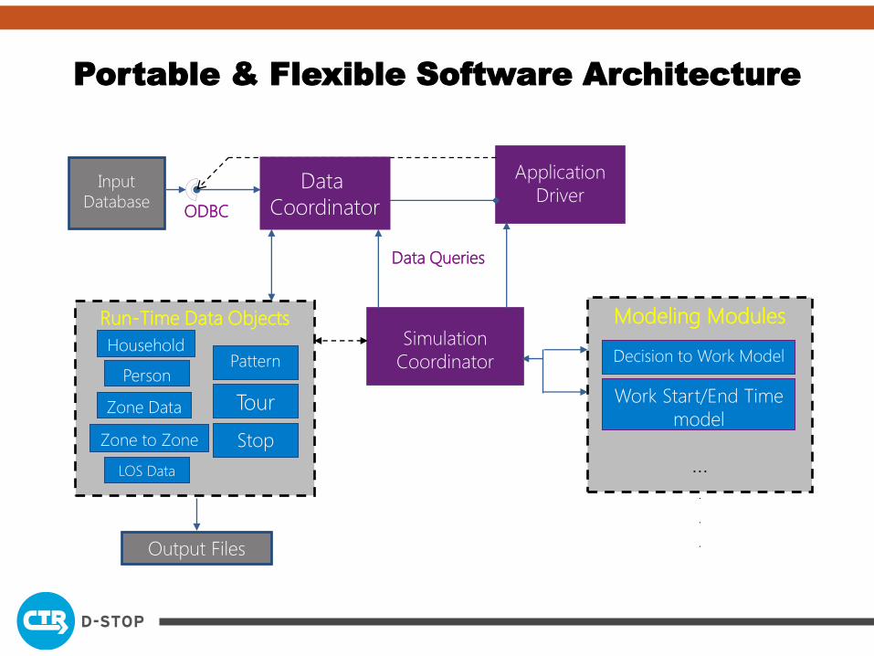
Portable & Flexible Software Architecture
ODBC
Run-Time Data Objects
Household
Person
Zone Data
LOS Data
Pattern
Tour
Stop
Output Files
Simulation
Coordinator
Modeling Modules
… .
.
.
Decision to Work Model
Work Start/End Time
model
Input
Database
Application
Driver
Data Queries
Zone to Zone
Data
Coordinator

Ability to Integrate and Enhance
• Successfully interfaced with
– Multi-period static assignment (the current four-step approach of SCAG)
– TRANSIMS and MATSim (second by second assignment of people and vehicles on networks), and
• Continuous-time evolutionary framework facilitates real-time dynamic integration of ABM and DTA models
• SimAGENT is successfully implemented in the LA region
• Existing SimAGENT code (CEMDAP, PopGen, CEMSELTS) is open source
• Being implemented currently in the New York region; selected based on behavioral realism and ability to accommodate CAVs
• Elements of system being used for long distance travel modeling by CDOT; UT-Austin working with CDOT

• One may develop the reduced form equations as below:
• Parameters to be estimated
• Latent utility differentials of all non-chosen alternatives with respect to the
chosen alternative
→ →
→ and
where and
Reduced Form Model and Estimation
)((
~
ξηcBcxb
ξηBcxb
ξηαscxbyU
S )
S
SS
)(,(MVN)(
ΣIDENΞ )
QGEQ
ccBcxb~yU
] , , ),Vech(),Vech(),Vech(),Vech([ δΣλ θφcbα
qggqgg qgmqgimqgi UUu
ggmqgImqgmqgqg miuuu
qggqgqg;,...,, 21u
qGqqq uuuu ,...,, 21
,)(
qqq uyyu
)(,...,)(,)( 21
Qyuyuyuyu Ω~,
~MVN
)~
(Β~yu
GEQ
)M BcxbB
(~
MΣIDENΞM Ω )(~
Qcc

Estimation
• Further, partition the vector and matrix which correspond to the mean
and variance of continuous, ordinal and count, and differenced utility elements
as follows:
B~
Ω~
) variablescontinuous of(mean 1)vector( ~~
QHBRB yy
) variablesnominal andcount ordinal, of(mean 1)vector~
( ~~
~~ EQBRB uu
) variablescontinuous theof e(covarianc )matrix( ~~
QHQH yyy RΩRΩ
) variablesnominal andcount ordinal, theof e(covarianc)matrix~~
( ~~
~~~ EQEQ uuu RΩRΩ
) variablesremaining and variablescontinuousbetween e(covarianc)matrix~
( ~~
~~ EQQHyy uu RΩRΩ
y
u
BB
B
y yu
yu u
Ω ΩΩ
Ω Ω

• : MNV density function of dimension QH with mean of and covariance
of
• : integral to evaluate the conditional likelihood of all ordinal, count, and
nominal variable outcomes for all Q individuals
• CML:
• Develop the likelihood function by decomposing the joint distribution of
into a product of marginal and conditional distributions
• given is MNV with mean and variance
Likelihood Function
)~,( uyyu
u~ y )~
(~~~ 1
~~~ yuuu ByBB
yy ΩΩ
uuuu ΩΩΩ-ΩΩ ~1
~~~~~~~
yyy
uplowQHfL ψuψB|y yy
~ Pr)
~,
~()( Ωλ
drffEQ
D
QH
r
),|()~
,~
( ~~~ uuyy BrB|y ΩΩ
)~
,~
( yyB|y ΩQHfyB
~
yΩ~
uplow ψuψ
~ Pr
uplowH
Q
q
Q
CML fL ,qqqq,qqy,qqy,qqqq ψuψB|y
~ Pr)
~,
~()( *2
1
1 1
Ωλ

Empirical Application

Framework