predicting field-scale solute transport using in situ measurements of soil hydraulic properties

Predicting Field-Scale Solute Transport Using In Situ Measurementsof Soil Hydraulic Properties

I. J. van Wesenbeeck* and R. G. Kachanoski

ABSTRACTPredicting unsaturated solute transport using measured hydraulic

parameters has been difficult due to the inherent variability of soilproperties, and the difficulty in obtaining accurate estimates of hydrau-lic properties in situ. The objective of this study was to determine ifin situ measurement of soil hydraulic conductivity, the a soil parameter,and the water content (B) vs. pressure head (h) relationship could beused to predict field-scale solute transport. A series of steady-statesolute transport experiments were conducted on a Fox sand (fine-loamyover sandy or sandy-skeletal, mixed, mesic Typic Hapludalf) soil inOntario, Canada. The transport of Cl~ under steady-state water fluxwas monitored in three separate experiments using solution samplers.Steady-state water flux densities applied at the soil surface were 9.72x 10-', 1.53 x H)"5, and 8.68 x lO"8 m s~', respectively, for thethree sites. After completion of the transport experiments at Site II,measurements of soil hydraulic conductivity and the a parameterwere made using the Guelph pressure inflltrometer (GPI) beside eachlocation and depth where solute breakthrough curves (BTCs) weremeasured, as well as at the soil surface. Undisturbed soil cores weretaken at each location where GPI measurements were made for estimat-ing the parameters in the 0(A) using van Genuchten's equations. TheGPI- and core-measured hydraulic parameters obtained at Site IIwere used to predict the field-scale solute travel time probability densityfunction (PDF) at the same site, and at Sites I and in using a stochastic-convective model. Observed solute travel time PDFs were predictedquite well at high surface water fluxes, which were close to the fieldsaturated hydraulic conductivity, K,s by both the GPI and core meth-ods. Both methods underpredicted the variability of the observedtravel time PDF.

PREDICTING UNSATURATED SOLUTE TRANSPORT USUlgfield-measured soil hydraulic parameters has been

difficult due to the inherent variability of soil properties.Significant variability of soil properties affecting solutetransport have been shown to occur within short distances(Biggar and Nielsen, 1976). Extensive variability infield-measured hydraulic parameters such as soil-waterpressure (Yeh et al., 1985a), hydraulic conductivity (Russoand Bresler, 1981), and soil water content (van Wesen-beeck and Kachanoski, 1988) has caused researchers toquestion the validity of using deterministic models fordescribing field-scale solute transport behavior. The useof field average values as deterministic model parametershas been shown to give poor agreement with field-scaleobservations (Parker and van Genuchten, 1984). There-fore, researchers have used the stochastic flow equationsand estimates of soil hydraulic conductivity and the soilparameter a to model unsaturated flow (Yeh et al.,1985a).

I.J. van Wesenbeeck, DowElanco, Environmental Fate, Bldg. 306-Az,9330 Zionsville Rd., Indianapolis, IN 46268; and R.G. Kachanoski, Dep.of Land Resource Science, Univ. of Guelph, Guelph, ON, Canada NIG2W1. Received 21 Feb. 1994. *Corresponding author.

Published in Soil Sci. Soc. Am. J. 59:734-742 (1995).

VAN WESENBEECK & KACHANOSKI: PREDICTING FIELD-SCALE SOLUTE TRANSPORT 735

Other researchers have developed mechanistic-sto-chastic models that preserve the classical concepts ofsolute transport while incorporating the inherent hori-zontal variability of hydraulic parameters at the fieldscale. Dagan and Bresler (1979) suggested a model forsteady-state unsaturated infiltration that involves dividingthe field into a series of parallel vertical soil or streamcolumns. Within each soil column, the hydraulic proper-ties are uniform with depth and solute transport is de-scribed by the CDE. Soil columns are assumed to beindependent, and hydraulic properties are assumed tovary stochastically with no solute passing from one col-umn to another. They assume that hydrodynamic disper-sion is insignificant so that the solute spread at the fieldscale is attributed solely to the variability of the localtravel times hi each of the parallel soil columns. Daganand Bresler then used the lognormal PDF of the measuredsaturated hydraulic conductivity (^at) and a set of scalingparameters to predict the PDF of solute concentrationsin a horizontal soil layer. Amoozegar-Fard et al. (1982)and Persaud et al. (1985) used similar conceptual modelsto model the effects of variable soil water velocity anddispersion on solute movement during infiltration. Jayneset al. (1988) calibrated a stream-column model for pre-dicting the leaching of a uniformly applied conservativetracer under flood irrigation. They used a probabilitydistribution function of solute velocities based on esti-mates of steady ponded infiltration rate, evaporation, andimmobile water content obtained from field measure-ments to predict Br ~ movement. Their model predictedmean Br~ movement quite well; however, the ability oftheir model to predict solute dispersion decreased withdepth. Their model is not strictly applicable to an unsatu-rated surface boundary condition since it is based on thevariability of preferential infiltration of surface pondedwater.

Few data sets exist where in situ measurements of soilhydraulic properties such as KfS, matric flux potential((pm), and volumetric water content (9V) vs. h relationshipwere made at the exact locations where solute transportproperties were measured under unsaturated steady-stateconditions. Wierenga et al. (1991) conducted a detailedhydraulic characterization of a field trench followed by atracer experiment; however, unsaturated flow parameterswere estimated from laboratory-determined water reten-tion curves. Of interest to a number of researchers isthe a parameter (ATsatCpnT1), which has been related to amean flow weighted capillary length scale (Philip, 1969).Few studies have provided detailed information on thespatial distributions of a (Russo, 1983; Unlu et al., 1990;Russo and Bouton, 1992).

The prediction of water and solute transport in thefield using models also depends on the reliability of insitu measurements of soil hydraulic properties. Althoughsignificant amounts of information are available on the

Abbreviations: GPI, Guelph pressure infiltrometer; ETC, breakthroughcurve; PDF, probability density function; CDE, convection-dispersionequation; TDK, time domain reflectometry; EC, electrical conductivity;ANOVA, analysis of variance.

spatial distribution of hydraulic conductivity, determin-ing the statistical properties of a has been difficult andhence little information exists (Yeh et al., 1985b). Re-cently, White and Sully (1992) discussed the distributionproperties of a in the field and its impact on stochasticmodeling.

The purpose of this study was to: (i) determine whetherin situ measurements of soil K& and the a parameter,and the Q(h) relationship obtained from undisturbed fieldcores, could be used to predict the distribution of 0V and(ii) to use the Dagan-Bresler stream tube model with aknown water flux, q, at the soil surface to estimate thePDF of observed solute travel tunes.

METHODS AND MATERIALSSolute Transport Experiments

The study site is at the Agriculture Canada Delhi researchstation near Delhi, Ontario. The soil is a well-drained, coarse-textured Typic Hapludalf (Fox series) exhibiting well-developedhorizonation, and characterized by significant variability inhorizon thickness. The surface Ap horizon has 85 to 90% sandcontent, compared with 90 to 95% sand in the top 0.2 m ofthe Bm horizon.

Steady-state unsaturated flow tracer experiments were con-ducted at three sites between 1988 and 1991. At Site I, 48porous ceramic cup solution samplers (5.0 by 2.0 cm diam.)were installed at both the 0.4- and 0.8-m depths. Samplerswere installed in two adjacent transects 0.1 m apart, at 0.2-mintervals, resulting in a 9.6-m-long transect of solution samplersfor each depth. Site I had been under continuous cultivationfor at least 50 yr, and was planted in corn when the experimentwas conducted in 1988. A constant flux density, q = 9.72 x10~6 m s"1, of water was applied continuously to the transectusing drip irrigation lines. The coefficient of variation of flowout of individual emitters was 6.5%. Emitters were spaced0.15 m apart along the lines, with the individual lines spacedO . l m apart. The density of the emitters was approximately67 m~2. The drip emitters were staggered to maximize theuniformity of water application. The entire water deliverysystem was shifted regularly during irrigation to randomizeany variations in water flow that existed between emitters.The wetted area extended for 1.0 m on either side and beyondthe ends of the transect.

Soil water content was nondestructively measured using theTDR method (Topp et al., 1980), and TDR transmission probesmade of 2-mm-diam. stainless steel rods. A total of 48 TDRprobes were installed at each of the 0.4- and 0.8-m depths.The transport zone was brought to steady-state water contentprior to the tracer application by preirrigation until the measuredsoil water content (0-0.8 m) no longer changed (»7 h).

Once steady-state water flux was achieved, irrigation wastemporarily stopped, and a uniform pulse of 58 g m'2 Cl~ inthe form of KC1 was applied by subdividing the plot into smallareas (0.8 m2) and spraying on equal quantities of the KC1tracer. After application of the KC1 tracer, approximately2 mm of irrigation water was applied to the plot using thesame hand sprayers to ensure that KC1 was moved off theirrigation lines and into the soil. Irrigation was then resumedand the Cl~ was leached through the soil profile using theirrigation system with the same flux density of water. Sampleswere collected from all solution samplers simultaneously atregular time intervals using an electric vacuum pump andmanifold system that distributed vacuum evenly to all the

736 SOIL SCI. SOC. AM. J., VOL. 59, MAY-JUNE 1995

samplers. Solution samples from selected sites were monitoredin the field for bulk EC, using a portable EC meter to determinewhen the main portion of the pulse had passed. Samples(1-2 mL) were collected in evacuated containers and analyzedfor Cl~ content using an autoanalyzer. In total, 1968 Cl~samples were analyzed for the two depths at Site I. Additionaldetails of the methods of soil solution sampling and datasummaries are given by Hamlen and Kachanoski (1992) andvan Wesenbeeck and Kachanoski (1991).

A series of tracer experiments similar to those describedfor Site I was conducted at Site II in the summer of 1989(Hamlen and Kachanoski, 1992). Site II is located approxi-mately 100 m southwest of Site I on the same soil type. Aset of 48 solution samplers (3.2 by 1.0 cm diam.) were installedat the 0.2- and 0.4-m depths, spaced at 0.2-m intervals, re-sulting in a 9.6-m-long transect. The site was maintained freeof vegetation by application of herbicide. Irrigation and pulseapplication methods were the same as those used for Site I.A steady-state surface water flux density, q = 1.53 X 10~5

m s~', was applied at the soil surface. A uniform pulse of102 g m~2 Cl~ was applied at the soil surface when steady-state6» was reached. Sample retrieval and Cl~ analysis were alsoperformed as outlined for Site I. A total of 3120 Cl~ sampleswere analyzed in total for the two depths at Site II.

A series of large-scale Cl~ and NOa~ tracer experimentswere conducted at Site III during the summer of 1991 (Younie,1993). Site HI is located approximately 50 m north of Site I.A set of 80 solution samplers (5.0 by 2.0 cm diam.) wereinstalled in paired 10 by 10 m plots, 40 in conventional-tillageplots and 40 in zero-tillage plots. Samplers were installed atthe 0.4-m depth and were evenly distributed between row andinterrow positions. The site had been planted in corn, but theexperiment was conducted in September after the crop hadbeen cut down. The plots were irrigated using the methodsdescribed for Site I and II; however, the average net appliedq, after correction for evaporation, was very low (8.68 x10~8 m s~') and therefore the experiment lasted for several

weeks. If a natural rainfall occurred, the daily water applicationwas adjusted to maintain an average daily water applicationofq=l .16 X 10~7 m s~l at the soil surface during the entireseason. The water flux at the surface was also corrected forevaporation, which was estimated for each day using the Priest-ley-Taylor model.

Estimation of Transport fromSoil Hydraulic Properties

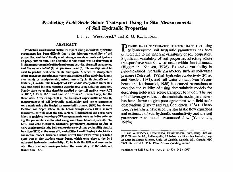
Guelph pressure infiltrometer measurements (Reynolds andElrick, 1990) were made for determination of K& (m h~') and(pm (m2 h"1) after completion of the solute transport experi-ments. The GPI measurement is based on a constant-head,single-ring infiltration measurement. The GPI is designed spe-cifically to measure Kfs and q>m at the surface of insertion withminimal disturbance to the soil surface itself. The design ofthe surface ring is convenient since it enables the removal ofan undisturbed core from within the area where the GPI esti-mates of ATfS and <pm were made (Fig. 1).

The GPI measurements were made by inserting the 10-cm-diam. sealed steel ring of the infiltrometer 5 cm into the soil,applying a constant head of water, and measuring water flowout of the permeameter during subsequent infiltration. The near-steady-state values of water flow out of the infiltrometer, Q(m3 h~'), were recorded for each of two applied heads (5 and10 cm). Estimates of Kfs and (pm were obtained using thetwo-head technique and the equations outlined in Reynoldsand Elrick (1990):

[1]

where a is the ring radius, H is the applied head, and G isa shape factor depending on the depth of insertion and thecross-sectional area of the surface ring.

Estimates of a were obtained from a = Kf,ym~l, with cpm

refill port

head space

small reservoir

pressure headindicator

vacuum port

water level

large reservoir

Fig. 1. Diagram of the Guelph pressure infiltrometer (GPI) apparatus.


given by

[2]where h = soil matric pressure head, K(h) = unsaturatedhydraulic conductivity as a function of matric pressure head,and -i|/i = initial soil matric pressure head. This methodresulted in some negative values of cpm at the 0.4-m depth.When negative values of (pra resulted from the two-head mea-surement, an average value of a for this soil was used tocalculate an estimate of (pm and KfS using the one-head technique(D.E. Elrick, 1993, personal communication).

The GPI measurements were made every 0.2 m, in a 9.6-m-long transect that was parallel and directly adjacent to thetransect of solution samplers at Site II. Thus, the center ofthe GPI measurement was approximately 5 cm away from theedge of the solution sampler. The GPI measurements werealso made at the 0.2- and 0.4-m depths adjacent to the locationswhere solute transport was measured using the solution sam-plers. This resulted in 48 estimates of Kfs and a at each ofthe surface and 0.2- and 0.4-m depths. The GPI measurementsat the 0.2- and 0.4-m depths were made by excavating theentire transect to the desired depth. The measurements couldhave been made without excavation by using the bore holepermeameter (Guelph permeameter) method.

Cores (5-cm diam., 5 cm long) were taken from within thearea enclosed by the sealed GPI ring at each location after theGPI measurements were completed at Site II. The undisturbedcores were taken to the lab for measurement of Km and thewater release curve, Q(h). The value of KM was determined oneach core (n = 48 per depth X 3 depths) using the constant-headmethod (Klute and Dirksen, 1986). The value of 0(/i) wasdetermined on the saturated cores using a standard pressureplate apparatus. Cores were placed in the pressure chamberand equilibrated at 10-, 25-, 50-, 100-, 333-, and 15000-cmpressure heads. Soil water content was determined gravimetri-cally at equilibrium pressure values. Bulk density was deter-mined from a final oven drying of the undisturbed cores. Thevan Genuchten parameters a and n were fitted to the Q(h)curves at each location using a nonlinear least squares optimiza-tion routine of the following equation (van Genuchten, 1980):

- ej i(6S - 9r) [1 + (a/i)"]1"1'"

where 0r = residual volumetric water content at h = —15000cm, 0S = saturated volumetric water content, 0(/z) = volumetricwater content at matric pressure head h, and a and n are fittedparameters of the 0(/i) curve. Only the parameters a and nwere fitted to Eq. [3] since the parameters 0S and 0r wereobtained from the water release curve directly.

Gardner's (1958) equation gives a relationship between hy-draulic conductivity and h ifKfs and a from the GPI are known:

K(h) = ATfsexp(-a/z) [4]A value of the equilibrium pressure head for a steady q at thesoil surface was obtained by assuming a unit gradient andsetting K(h) = q in Eq. [4] and rearranging to solve for h:

_ \n(q)-ln(Kh)a [5]

The value of h obtained from Eq. [5] was then substitutedinto van Genuchten's model of Q(h) (Eq. [3]) to solve for thesteady-state 0V for the given steady-state q. This method ofobtaining 9V relies on information obtained from the water

release curve and from GPI estimates of Kfs and a, and isreferred to as the GPI method for comparison purposes.

Van Genuchten's (1980) closed form equation for hydraulicconductivity as a function of pressure head is given as follows:

K(h) ={[I-(ah)"-1 (I + ah)Tm}-ml 2

[1 + (ah)"] mil [6]

For each core, Eq. [6] was solved for the steady-state hassociated with a steady-state q by setting K(h) = q. The valueof h obtained from Eq. [6] was used to predict a steady-state 9Vusing Eq. [3]. Estimates of a were also obtained by numericallyintegrating the area under the K(h) curve (Eq. [6]). This methodalways results in a positive value for cpm and a since theparameters are determined from equations derived from theempirically based relationship for 9(/i) and K(h) given by Eq.[3] and [6]. This method relies solely on information obtainedfrom the water release curve and is referred to as the coremethod for comparison purposes.

The general approach to estimating the solute travel timePDFs was similar to the stream-column model suggested byDagan and Bresler (1979) and therefore invokes the followingassumptions regarding the transport process: (i) the hydraulicproperties controlling solute transport vary horizontally acrossthe field but not within the measurement depth, (ii) each streamcolumn is independent and therefore there is no transport ofsolutes between columns, and (iii) solute transport within eachstream column can be described by a simple piston displacementmodel (i.e., local dispersion within a stream tube is negligible).

Dagan and Bresler (1979) suggested that the variability ofhydraulic parameters can be described by a random functionof hydraulic conductivity, £(0V). For steady, unsaturated waterflow and unit hydraulic gradient, AT(9») = q, where q = surfacewater flux density. Also, for steady-state flow, the averagelinear pore water velocity, v, is estimated by

v = q^ [7]The depth of solute migration, x, for a simple piston displace-ment model is

x = vt [8]where t is time. The mean solute travel time for a single streamcolumn can be given by

t = xQvq'1 [9]If the surface applied q is constant, then for a given x thefield-scale PDF of solute travel times depends only on thePDF of 0V.

This method assumes that at the local scale the entire wettedmatrix contributes to the transport of solutes and that themeasured 9V and the transport volume 9. are equal. The transportvolume is defined as the portion of the matrix that is contributingto flow and is calculated using

[10]

where robs is the measured solute travel time to the depth x.Equation [9] gives an estimate of the average solute travel

time, t, at the location where 0V is measured. The observedsolute travel time at a given location will be described by aprobability distribution of values because of local-scale disper-sion. Thus, for comparison purposes, the predicted values oft from the GPI and core methods were compared with estimatesof the local-scale average and peak travel times from the localBTC measured at the same location.

Estimates of the steady-state 0V for each of the 48 individual

738 SOIL SCI. SOC. AM. } . , VOL. 59, MAY-JUNE 1995

locations in space obtained from Eq. [3] and [5] (GPI method)and Eq. [3] and [6] (core method) were used in Eq. [9] toobtain estimates of average local-scale solute travel times forthe desired depths. Values of 6V for a particular depth wereobtained by averaging the point estimates of 9V from the soilsurface to the 20- or 40-cm depth. Sets of 48 local-scale averagetravel times were generated for each of the measurement depthsand for each of the surface flux densities of water, q, used inthe transport experiments at Sites I, II, and HI. Cumulativeprobability histograms of solute travel times were plotted fora given depth and q. Parameters of the solute travel time PDFsestimated from hydraulic properties measured at Site n werethen compared with the PDFs of average local-scale solutetravel times measured at the same site and Sites I and in.

Chloride BTCs measured using solution samplers, C(j,t),where t = time (h) and j = spatial location, were analyzedusing the method of moments. The zeroth moment, M(J), isrelated to the solute mass recovery at j and was calculatedfrom

[11]

10

= I C(j,t)dt

Solute mass recovery was estimated as q M(j).The first moment, fcO'), is the center of mass or average

(centroid) value of the ETC, and was calculated at each j fromthe normalized ETC using

C(j,t)[M(j)]-*tdt [12]

The variance of the ETC, V\j), was also calculated ateach location as the first relative moment about tc(j), using

it [13]The modal travel time of the observed solute BTCs, tp, was

also measured as the time at which die peak solute concentrationoccurred.

RESULTS AND DISCUSSIONInfiltrometer- and Core-Measured

Hydraulic ParametersTable 1 shows the average GPI-measured hydraulic

parameters (Kfs, (pm, and a), and core-measured K& atSite n. Probit plots of the hydraulic parameters indicatedthat they were lognormally distributed in space and there-fore the values shown in Table 1 were calculated as themean and variance of a lognormal distribution. AverageKk and tfsat at the soil surface were 7.78 x 10~5 m s"1

and 9.72 x 10~5 m s"1, respectively. These values aresignificantly greater than the highest applied surface qof 1.53 X 10~5 m s"1 used in the tracer experiments.

1010

10"

10

10110

10

10"

104 6

Distance (m)10

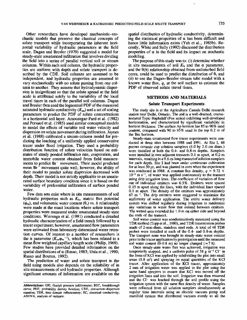
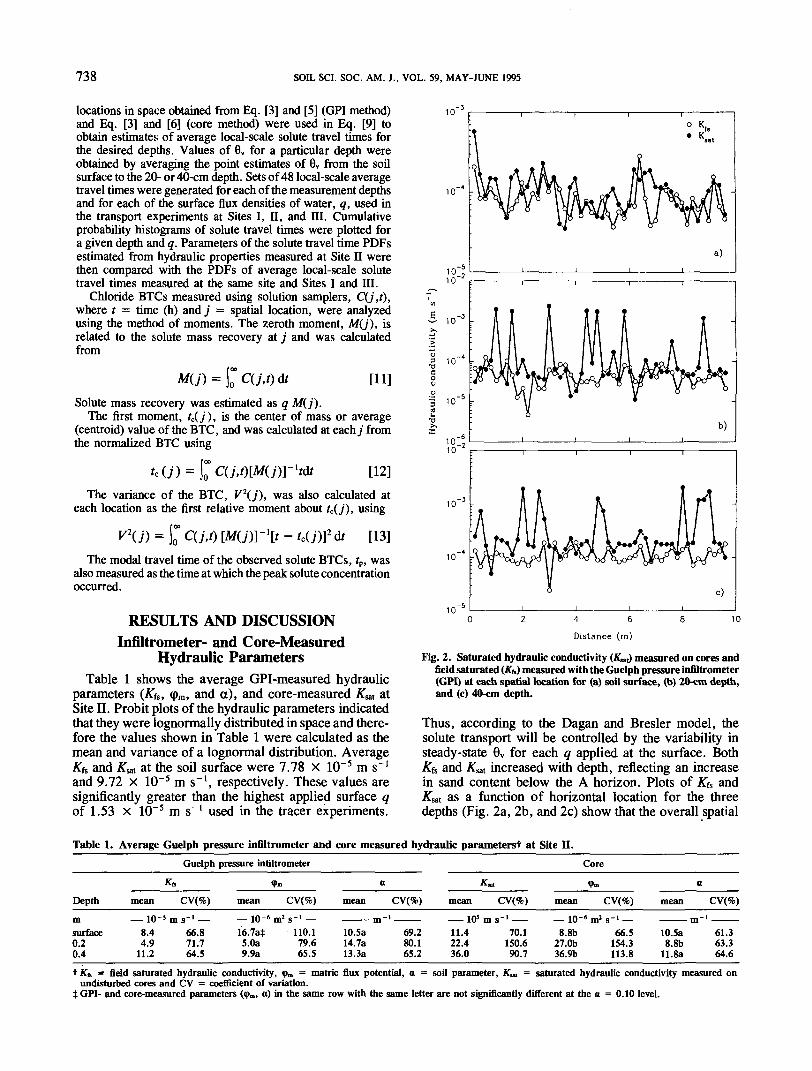
Fig. 2. Saturated hydraulic conductivity (K^ measured on cores andfield saturated (Kt,) measured with the Guelph pressure infiltrometer(GPI) at each spatial location for (a) soil surface, (b) 20-cm depth,and (c) 40-cm depth.

Thus, according to the Dagan and Bresler model, thesolute transport will be controlled by the variability insteady-state 6V for each q applied at the surface. Both.Kfs and Ksat increased with depth, reflecting an increasein sand content below the A horizon. Plots of Kts and£sat as a function of horizontal location for the threedepths (Fig. 2a, 2b, and 2c) show that the overall spatial

Table 1. Average Guelph pressure infiltrometer and core measured hydraulic parameterst at Site n.Guelph pressure infiltrometer Core

Depth CV(%) CV(%) CV(%) CV(%) CV(%) CV(%)

surface0.20.4

10-' ms- '8.4 66.84.9 71.7

11.2 64.5

6

16.7at5.0a9.9a

m2 s-1 —110.179.665.5

lO.Sa14.7a13.3a

_-i69.280.165.2

10s

11.422.436.0

70.1150.690.7

— 10-' m2 :8.8b

27.0b36.9b

_,

66.5154.3113.8

lO.Sa8.8b

11. 8a

m-1

61.363.364.6

= saturated hydraulic conductivity measured ontK& = field saturated hydraulic conductivity, (pm = matric flux potential, a = soil parameter,undisturbed cores and CV = coefficient of variation.| GPI- and core-measured parameters (ipm, <x) in the same row with the same letter are not significantly different at the a = 0.10 level.


Table 2. Correlation coefficients between measured soil hydraulicproperties^ for the soil surface and the 0.2- and 0.4-m depths.

10'

JffiKM

<PmOGPIOcorc

K*KM

<PmOOPIOcors

Kf,KM9mOGPI<«<»«

•*MI *»iat ^Pm

Soil surface1.00 0.23 0.15

1.00 0.201.00

0.2-m depth1.00 -0.02 0.19

1.00 0.161.00

0.4-m depth1.00 -0.05 -0.12

1.00 -0.011.00

OOPI

0.75***0.00

-0.38t1.00

0.32f0.12

-0.52t1.00

o.sot-0.13-0.44t

1.00

<>«»,

-0.010.33t0.22

-0.111.00

0.160.080.27

-0.161.00

0.11-0.08

0.36t-0.14

1.00t, *** Significantly correlated at the 0.10 and 0.001 levels, respectively.tKh = field saturated hydraulic conductivity, <pm = matrix flux potential,

OGPI = soil parameter estimated by the Guelph pressure infiltrometer,Ocon = soil parameter estimated from 0(/i) relationship.

pattern of the measured parameters within a depth arereasonably consistent, but the correlation coefficient be-tween Kfs and KM was low for all measurement depths(Table 2).

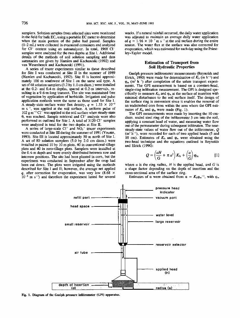
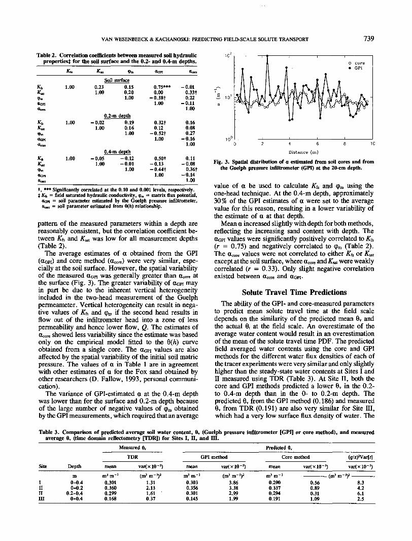
The average estimates of a obtained from the GPI(OGPI) and core method (aCOre) were very similar, espe-cially at the soil surface. However, the spatial variabilityof the measured aGpi was generally greater than Ocore atthe surface (Fig. 3). The greater variability of OGPI mayin part be due to the inherent vertical heterogeneityincluded in the two-head measurement of the Guelphpermeameter. Vertical heterogeneity can result in nega-tive values of K& and q>m if the second head results inflow out of the infiltrometer head into a zone of lesspermeability and hence lower flow, Q. The estimates ofOcore showed less variability since the estimate was basedonly on the empirical model fitted to the 9(/z) curveobtained from a single core. The CGPI values are alsoaffected by the spatial variability of the initial soil matricpressure. The values of a in Table 1 are in agreementwith other estimates of a for the Fox sand obtained byother researchers (D. Fallow, 1993, personal communi-cation).

The variance of GPI-estimated a at the 0.4-m depthwas lower than for the surface and 0.2-m depth becauseof the large number of negative values of <pm obtainedby the GPI measurements, which required that an average

10

10"

o core• GPI

4 6

Distance (m)

10

Fig. 3. Spatial distribution of a estimated from soil cores and fromthe Guelph pressure infiltrometer (GPI) at the 20-cm depth.

value of a be used to calculate K& and (pm using theone-head technique. At the 0.4-m depth, approximately30% of the GPI estimates of a were set to the averagevalue for this reason, resulting in a lower variability ofthe estimate of a at that depth.

Mean a increased slightly with depth for both methods,reflecting the increasing sand content with depth. TheOGPI values were significantly positively correlated to Kts(r = 0.75) and negatively correlated to (pm (Table 2).The ttcore values were not correlated to either K& or K^texcept at the soil surface, where acore and KM were weaklycorrelated (r = 0.33). Only slight negative correlationexisted between acore and

Solute Travel Time PredictionsThe ability of the GPI- and core-measured parameters

to predict mean solute travel time at the field scaledepends on the similarity of the predicted mean 9V andthe actual 0t at the field scale. An overestimate of theaverage water content would result in an overestimationof the mean of the solute travel time PDF. The predictedfield averaged water contents using the core and GPImethods for the different water flux densities of each ofthe tracer experiments were very similar and only slightlyhigher than the steady-state water contents at Sites I andH measured using TDK (Table 3). At Site II, both thecore and GPI methods predicted a lower 9V in the 0.2-to 0.4-m depth than in the 0- to 0.2-m depth. Thepredicted 0V from the GPI method (0. 186) and measured0V from TDR (0.191) are also very similar for Site HI,which had a very low surface flux density of water. The

Table 3. Comparison of predicted average soil water content, 0, (Guelph pressure infiltrometer [GPI] or core method), and measuredaverage 0, (time domain reflectometry [TDR]) for Sites I, II, and m.

Measured 6.

TDR

Site

IIInm

Depth

m0-0.40-0.2

0.2-0.40-0.4

mean

m3m-3

0.3010.3600.2990.168

var(xlO-3)

(m3 m-3)2

1.312.131.610.37

GPImean

0.3030.3560.3010.145

method

var(xlO-3)

(m3 m-3)2

3.863.382.991.99

Predicted 8.

Core

mean

m 3 m- 3

0.2900.3370.2940.191

method

var(xlO"3)

—————— (m3

0.560.890.311.09

(q/xfVailt]var(xlO-3)

m-3)2

8.34.26.12.5


Table 4. Mean, EM, and variance, V2[t], of measured and predicted (Guelph pressure infiltrometer [GPI] or a core method) peak (tp)and centroid (fc) solute travel time probability density functions for transport experiments at Sites I, n, and III.

Measured

Site

IIInIII

Water flux density

m s"'9.72 x 10-'1.53 x 10-5

1.53 x 10-5

8.68 x II)-8

Depth

m0.40.20.40.4

tf

3.34at1.19a2.42ab

263a

tc

3.37a1.31b2.62a

GPI predicted

tp

3.30a1.25ab2.30b

165b

f.-h —————

3.25a1.24ab2.23b

203b

Core predicted

tf

3.20a1.30ab2.50b

170b

fc

3.35a1.26ab2.29b

180b

Measured

peak

1.080.060.24

4127

centroid

———— h2

0.840.060.32

Predicted

GPI

0.300.050.12

3327

core

0.170.030.08

625

t Values within a row with the same letter are not significantly different at the 0.10 level.

core-predicted 0V for Site III was substantially lower thanthe measured 9V (TDR) and the GPI-predicted 6V.

Although the mean predicted water contents suggestthat the predicted travel tune PDFs should overestimatethe observed mean travel tune, the travel times predictedusing the GPI and core methods generally underestimatedthe measured average travel time of the centroid, andto some extent the time to the peak of the observedlocal-scale BTCs (Table 4). However, the accuracy de-pended on the flow rate and depth.

Mean peak travel time for all spatial locations, E[fp],of the measured BTCs were less than the mean centroidtravel time, E[rc], obtained from moment analysis, proba-bly because of die skewed nature of the observed soluteBTCs. For significantly skewed BTCs, the centroid maynot give a physically meaningful average travel time.Many of the local-scale solute BTCs were positivelyskewed and the Ot calculated from the centroid travel timewas greater than the measured 0V, which is physicallyimpossible. Transport volumes calculated using the esti-mated peak travel time were lower than those calculatedusing the centroid mean travel time and were similar tothe measured 0V. Since the majority of the observedBTCs for all the tracer experiments at this site haveexhibited skewness (average skewness coefficient rangingfrom 0.14 to 1.51 for the tracer experiments), the traveltime to the peak solute concentration was considered tobe a better estimate of the average travel time of the bulk

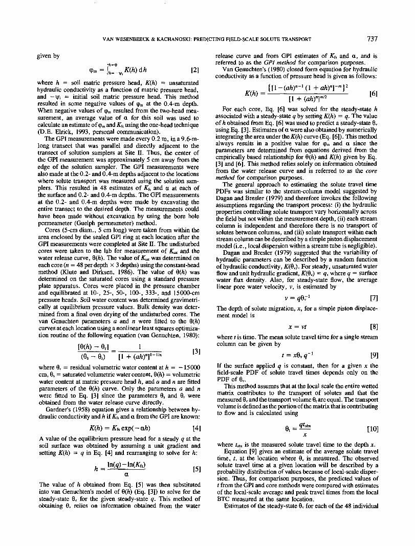
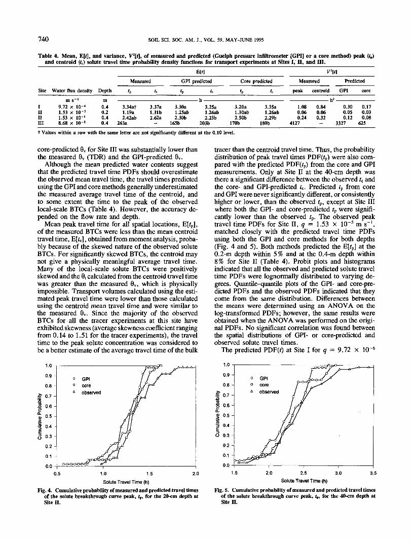
tracer than the centroid travel time. Thus, the probabilitydistribution of peak travel times PDF(rp) were also com-pared with the predicted PDF(rp) from the core and GPImeasurements. Only at Site II at the 40-cm depth wasthere a significant difference between the observed tc andthe core- and GPI-predicted tc. Predicted tp from coreand GPI were never significantly different, or consistentlyhigher or lower, than the observed tp, except at Site HIwhere both the GPI- and core-predicted tp were signifi-cantly lower than the observed tp. The observed peaktravel tune PDFs for Site II, q = 1.53 x 10~5 m s"1,matched closely with the predicted travel time PDFsusing both the GPI and core methods for both depths(Fig. 4 and 5). Both methods predicted the E[tp] at the0.2-m depth within 5% and at the 0.4-m depth within8% for Site II (Table 4). Probit plots and histogramsindicated that all the observed and predicted solute traveltime PDFs were lognormally distributed to varying de-grees. Quantile-quantile plots of the GPI- and core-pre-dicted PDFs and the observed PDFs indicated that theycome from the same distribution. Differences betweenthe means were determined using an ANOVA on thelog-transformed PDFs; however, the same results wereobtained when the ANOVA was performed on the origi-nal PDFs. No significant correlation was found betweenthe spatial distributions of GPI- or core-predicted andobserved solute travel times.

The predicted PDF(0 at Site I for q = 9.72 x 10~6

o.o0.5

Solute Travel Time (h)Fig. 4. Cumulative probability of measured and predicted travel times

of the solute breakthrough curve peak, tp, for the 20-cm depth atSite n.

0.01.5 2.0 2.5


of the solute breakthrough curve peak, tp, for the 40-cm depth atSite n.


0.01.5 2.0 2.5 3.0 3.5 4.0 4.5


of the solute breakthrough curve peak, tf, for the 40-cm depth atSite I.

m s"1 (Fig. 6) based on hydraulic properties measuredat Site II predicted the E[tp] within 3% using the GPImethod and within 1 % for the core method. The averagetravel time of the centroid was overestimated and thetravel tune variance was again consistently underesti-mated by both methods.

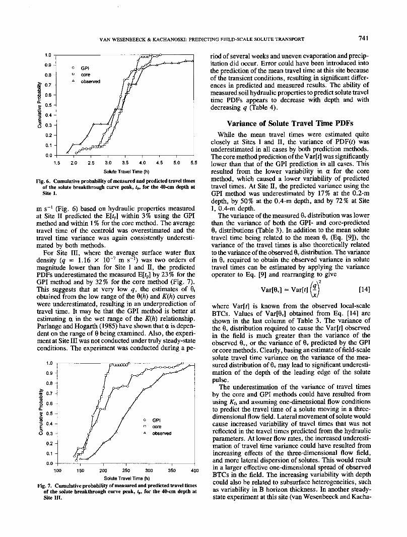
For Site III, where the average surface water fluxdensity (q = 1.16 X 10~7 m s"1) was two orders ofmagnitude lower than for Site I and n, the predictedPDFs underestimated the measured E[rp] by 23 % for theGPI method and by 32% for the core method (Fig. 7).This suggests that at very low q, the estimates of 9tobtained from the low range of the Q(h) and K(h) curveswere underestimated, resulting in an underprediction oftravel time. It may be that the GPI method is better atestimating a in the wet range of the K(h) relationship.Parlange and Hogarth (1985) have shown that a is depen-dent on the range of 0 being examined. Also, the experi-ment at Site III was not conducted under truly steady-stateconditions. The experiment was conducted during a pe-

o.o100 150 350 400200 250 300


of the solute breakthrough curve peak, tp, for the 40-cm depth atSite m.

riod of several weeks and uneven evaporation and precip-itation did occur. Error could have been introduced intothe prediction of the mean travel time at this site becauseof the transient conditions, resulting in significant differ-ences in predicted and measured results. The ability ofmeasured soil hydraulic properties to predict solute traveltime PDFs appears to decrease with depth and withdecreasing q (Table 4).

Variance of Solute Travel Time PDFsWhile the mean travel tunes were estimated quite

closely at Sites I and n, the variance of PDF(f) wasunderestimated in all cases by both prediction methods.The core method prediction of the Varff] was significantlylower than that of the GPI prediction in all cases. Thisresulted from the lower variability in a for the coremethod, which caused a lower variability of predictedtravel times. At Site n, the predicted variance using theGPI method was underestimated by 17% at the 0.2-mdepth, by 50% at the 0.4-m depth, and by 72% at SiteI, 0.4-m depth.

The variance of the measured Ov distribution was lowerthan the variance of both the GPI- and core-predicted6V distributions (Table 3). In addition to the mean solutetravel time being related to the mean Gv (Eq. [9]), thevariance of the travel tunes is also theoretically relatedto the variance of the observed 0V distribution. The variancein 6V required to obtain the observed variance hi solutetravel times can be estimated by applying the varianceoperator to Eq. [9] and rearranging to give

/ \2

Var[6»] = VarW P [14]

where Var[t] is known from the observed local-scaleBTCs. Values of Var[0v] obtained from Eq. [14] areshown in the last column of Table 3. The variance ofthe 6V distribution required to cause the Var[f] observedin the field is much greater than the variance of theobserved 6V, or the variance of 0V predicted by the GPIor core methods. Clearly, basing an estimate of field-scalesolute travel time variance on the variance of the mea-sured distribution of Ov may lead to significant underesti-mation of the depth of the leading edge of the solutepulse.

The underestimation of the variance of travel timesby the core and GPI methods could have resulted fromusing K& and assuming one-dimensional flow conditionsto predict the travel tune of a solute moving in a three-dimensional flow field. Lateral movement of solute wouldcause increased variability of travel times that was notreflected in the travel times predicted from the hydraulicparameters. At lower flow rates, the increased underesti-mation of travel time variance could have resulted fromincreasing effects of the three-dimensional flow field,and more lateral dispersion of solutes. This would resultin a larger effective one-dimensional spread of observedBTCs in the field. The increasing variability with depthcould also be related to subsurface heterogeneities, suchas variability in B horizon thickness. In another steady-state experiment at this site (van Wesenbeeck and Kacha-


noski, 1994), where the three-dimensional resident con-centration plume was measured in a trench experiment,significant preferential movement of solutes and shieldedzones were observed and related to the variability inB horizon thickness. The field variability violates theassumptions required by the prediction method, whichare that flow is one dimensional, that there is a unit verticalgradient, and that q is uniform at all depths as well asat the soil surface.

The accurate prediction of the peak travel time fromthe hydraulic properties for high q, however, suggeststhat die PDF of hydraulic properties measured at Siten are representative of the Fox series soil at high soilwater contents (low tension range) and can be used topredict peak solute travel times at other locations in thefield.

CONCLUSIONSHydraulic properties measured at Site n were success-

fully used to predict the peak solute travel time at anothersite in the same soil type with a different water fluxdensity applied at the surface. The PDFs of solute traveltimes were predicted reasonably well using measuredhydraulic properties and assumptions of one-dimensionalflow for surface q that were close to K{s [the low tensionrange of the Q(fi) and K(h) curves]. The failure of thismethod at low q [high tension range of the K(h) relation-ship] was probably due to the lack of one-dimensionalflow with increasing depth and decreasing flux densityof water. In addition, the estimates of the hydraulic parame-ters are more likely to be accurate at high 0V (closer tosaturation) in the soil.

The variance of solute travel times were consistentlyunderpredicted using both the GPI and core methods.In addition, the core method, with its lower variabilityof a estimates, predicted lower variability of travel timesthan did the GPI method. The underprediction of thevariance of PDF(f) would have little effect on predictingthe mean arrival time of a contaminant, but would affectthe prediction of early time of arrival.

The similarity in the estimated average a using GPIand core methods is encouraging. The value of a has beenused by numerous researchers to quantify the relativecontributions of gravity vs. capillarity on unsaturatedone-, two-, and three-dimensional flow of water. Thus,average (integral) estimates of flow contributions fromcapillarity and gravity seem to be reasonably well pre-dicted at this site by scaling the 9(/t) curve to estimateK(h) using the equations developed by van Genuchten(1980).

predicting field-scale solute transport using in situ measurements of soil hydraulic properties

Documents