precise measurement of solar neutrinos with super
TRANSCRIPT

Precise Measurement of Solar Neutrinos
with
Super-Kamiokande III
Motoyasu Ikeda
December 16 2009

Abstract
New solar neutrino measurements with the Super-Kamiokande detector are reported. The mainmotivation of this thesis is to observe the spectrum distortion of solar neutrinos caused by thematter effect of neutrino oscillation in the Sun (MSW effect).
The data for this thesis were taken between August 2006 and August 2008, during the thirdphase of Super-Kamiokande (SK-III). Two neutrino samples are used in this thesis. The firstone with total electron energy between 6.5 and 20MeV has a total livetime of 547.9 days. Thesecond, with total electron energy between 4.5 and 6.5MeV has a total livetime of 298.2 daysafter rejecting high background periods caused by radioactive impurities accidentally injectedinto the detector.
With improved detector calibrations, a full detector simulation, and analysis methods, thesystematic uncertainty on the total neutrino flux is estimated to be ±2.3%, which is abouttwo thirds of the systematic uncertainty in the first phase of Super-Kamiokande (SK-I). Theobserved 8B solar flux in the 5.0 to 20MeV electron energy region is 2.28± 0.04 (stat.) ± 0.05(sys.) ×106cm−2sec−1, in agreement with previous measurements. The day-night asymmetryis measured to be ADN = −0.057 ± 0.031(stat.)±0.013(sys.). In the 4.5-5.0 MeV region, theobserved flux is 2.14+0.56
−0.54 (stat) ×106cm−2sec−1 and is consistent with the flux in the 5.0-20MeVregion.
A global oscillation analysis is carried out using SK-I, II, and III, and is combined with theresults of other solar neutrino experiments. The best-fit oscillation parameters are obtained withthe world’s best accuracy as sin2 θ12 = 0.29+0.024
−0.011 and ∆m212 = 6.03+1.21
−1.67 × 10⁻⁵eV 2. Combinedwith KamLAND result, the best-fit oscillation parameters are found to be sin2 θ12 = 0.304+0.017
−0.016
and ∆m212 = 7.59+0.12
−0.39×10⁻⁵eV 2. This parameter region corresponds to a 8B flux of 5.08+0.10−0.07×
106cm−2sec−1.The χ2 value of spectrum fit with the solar plus KamLAND best-fit prediction is 26.7/20d.o.f.
which is slightly better than 27.7/20d.o.f. with a flat shape. Although, this result is notstatistically significant, it is estimated that the improved calibration and analysis methods willgive a sensitivity of 3σ level discovery of the spectrum distortion within a few years, togetherwith re-analysis of the SK-I data.

Acknowledgements
First of all, I would like to express my great gratitude to Prof. Y. Takeuchi for giving me theexcellent opportunity of studying the solar neutrino at Super-Kamiokande. This thesis wouldnever exist without his support and encouragement.
I would like to appreciate Prof. Y. Suzuki for giving me the opportunity of studying in theSuper-Kamiokande experiment.
I would like to extend my gratitude to LOWE members, Prof. M. Nakahata, Prof. Y.Koshio, Prof. A. Takeda, Prof. H. Sekiya, Prof. S. Yamada, Prof. H. Watanabe, Prof. M.Sakuda Prof. H. Ishino Prof. Y. Fukuda Prof. M. Vagins, Prof. M. Smy, Prof. K. Martens,Prof. C. Shaomin, T. Iida, K. Ueno, T. Yokozawa, K. Bays, Andrew, Jordan, Dr. J. P. Cravens,Dr. L. Marti, Dr. J. Schuemann, H. Zhang, and B. Yang.
I would like to thank Kamkoka members who encouraged me for all the time, Prof. K. Abe,Prof. Y. Hayato, Prof. J. Kameda, Prof. K. Kobayashi, Prof. M. Miura, Prof. S. Mine, Prof. S.Moriyama, Prof. S. Nakayama, Prof. Y. Obayashi, Prof. H. Ogawa, Prof. M. Shiozawa, Prof.S. Tasaka, Prof. M. Yamashita, Dr. A. Minamino, Dr. Y. Takenaga, Dr. G. Mitsuka, Dr. H.Nishino, Dr. R. Wendell, Dr. M. Litos, Dr. J. L. Raaf, Dr. O. Simard, Dr. K. Hiraide, Dr. A.Minamino, K. Ueshima, C. Ishihara, N. Okazaki, D. Ikeda, T. Tanaka, Y. Furuse, Y. Idehara,D. Motoki T.F. McLachlan, S. Hazama, Y. Nakajima, Y. Yokosawa, Y. Kozuma, T. Hokama,H. Nishiie, A. Shinozaki, K. Iyogi, Maggie, Patrick, Y. Heng, P. Mijakowski, M. Dziomba, K.Connolly, and Prof. C. K. Jung.
Finally, I would like to express my greatest appreciation and gratitude to my family, relatives,all my friends, and K. Nagaoka.
1

Contents
1 Introduction 4
2 Physics Background 52.1 Solar neutrino and the Standard Solar Model . . . . . . . . . . . . . . . . . . . . 52.2 Energy spectrum of 8B . . . . . . . . . . . . . . . . . . . . . . . . . . . . . . . . . 102.3 Neutrino Oscillation of Solar Neutrinos . . . . . . . . . . . . . . . . . . . . . . . . 122.4 Solar Neutrino Experiment . . . . . . . . . . . . . . . . . . . . . . . . . . . . . . 142.5 Motivation and strategies of this thesis . . . . . . . . . . . . . . . . . . . . . . . . 16
3 Super-Kamiokande Detector 203.1 Detector outline . . . . . . . . . . . . . . . . . . . . . . . . . . . . . . . . . . . . 203.2 20-inch PMT . . . . . . . . . . . . . . . . . . . . . . . . . . . . . . . . . . . . . . 203.3 Data acquisition (DAQ) system . . . . . . . . . . . . . . . . . . . . . . . . . . . . 213.4 Water purification system . . . . . . . . . . . . . . . . . . . . . . . . . . . . . . . 27
4 Event reconstruction 304.1 Vertex reconstruction . . . . . . . . . . . . . . . . . . . . . . . . . . . . . . . . . 304.2 Direction reconstruction . . . . . . . . . . . . . . . . . . . . . . . . . . . . . . . . 324.3 Energy reconstruction . . . . . . . . . . . . . . . . . . . . . . . . . . . . . . . . . 32
5 Simulation 375.1 Outline of detector simulation . . . . . . . . . . . . . . . . . . . . . . . . . . . . . 375.2 New modeling of water condition . . . . . . . . . . . . . . . . . . . . . . . . . . . 395.3 Tunable input parameters . . . . . . . . . . . . . . . . . . . . . . . . . . . . . . . 41
6 Calibration 436.1 Outline of detector calibrations . . . . . . . . . . . . . . . . . . . . . . . . . . . . 436.2 Timing calibration . . . . . . . . . . . . . . . . . . . . . . . . . . . . . . . . . . . 446.3 Water Transparency Measurement . . . . . . . . . . . . . . . . . . . . . . . . . . 516.4 TBA tuning and Q.E. measurement by Ni calibration . . . . . . . . . . . . . . . 526.5 DT calibration . . . . . . . . . . . . . . . . . . . . . . . . . . . . . . . . . . . . . 536.6 LINAC Calibration . . . . . . . . . . . . . . . . . . . . . . . . . . . . . . . . . . . 546.7 Energy scale . . . . . . . . . . . . . . . . . . . . . . . . . . . . . . . . . . . . . . . 576.8 Energy resolution . . . . . . . . . . . . . . . . . . . . . . . . . . . . . . . . . . . . 636.9 Angular resolution . . . . . . . . . . . . . . . . . . . . . . . . . . . . . . . . . . . 63
2

7 Data Analysis 677.1 Monitoring of Radon level . . . . . . . . . . . . . . . . . . . . . . . . . . . . . . . 677.2 Run definition . . . . . . . . . . . . . . . . . . . . . . . . . . . . . . . . . . . . . . 677.3 Noise reduction . . . . . . . . . . . . . . . . . . . . . . . . . . . . . . . . . . . . . 697.4 Reduction for solar ν analysis . . . . . . . . . . . . . . . . . . . . . . . . . . . . . 727.5 Summary of Reduction step . . . . . . . . . . . . . . . . . . . . . . . . . . . . . . 86
8 Signal extraction 898.1 Solar angle fitting . . . . . . . . . . . . . . . . . . . . . . . . . . . . . . . . . . . . 898.2 How to get Yi . . . . . . . . . . . . . . . . . . . . . . . . . . . . . . . . . . . . . . 91
9 Systematic Uncertainties 949.1 Energy scale . . . . . . . . . . . . . . . . . . . . . . . . . . . . . . . . . . . . . . . 949.2 Energy resolution . . . . . . . . . . . . . . . . . . . . . . . . . . . . . . . . . . . . 949.3 8B spectrum . . . . . . . . . . . . . . . . . . . . . . . . . . . . . . . . . . . . . . . 959.4 Angular resolution . . . . . . . . . . . . . . . . . . . . . . . . . . . . . . . . . . . 959.5 Vertex shift . . . . . . . . . . . . . . . . . . . . . . . . . . . . . . . . . . . . . . . 959.6 Reduction . . . . . . . . . . . . . . . . . . . . . . . . . . . . . . . . . . . . . . . . 969.7 Spallation cut . . . . . . . . . . . . . . . . . . . . . . . . . . . . . . . . . . . . . . 969.8 Gamma ray cut . . . . . . . . . . . . . . . . . . . . . . . . . . . . . . . . . . . . . 979.9 Background shape . . . . . . . . . . . . . . . . . . . . . . . . . . . . . . . . . . . 979.10 Signal extraction method . . . . . . . . . . . . . . . . . . . . . . . . . . . . . . . 979.11 Cross section . . . . . . . . . . . . . . . . . . . . . . . . . . . . . . . . . . . . . . 999.12 Further quality cut for the lowest energy region . . . . . . . . . . . . . . . . . . . 999.13 Summary of systematic uncertainty . . . . . . . . . . . . . . . . . . . . . . . . . . 99
10 Result 102
11 Oscillation Analysis 11111.1 Spectrum fit . . . . . . . . . . . . . . . . . . . . . . . . . . . . . . . . . . . . . . . 11111.2 Time-Variation Analysis . . . . . . . . . . . . . . . . . . . . . . . . . . . . . . . . 11311.3 Oscillation constraint from SK . . . . . . . . . . . . . . . . . . . . . . . . . . . . 115
12 Discussion 11612.1 Global oscillation analysis . . . . . . . . . . . . . . . . . . . . . . . . . . . . . . . 11612.2 Comparison of Winter and Ortiz 8B spectrum . . . . . . . . . . . . . . . . . . . . 11912.3 Comparison with other results . . . . . . . . . . . . . . . . . . . . . . . . . . . . . 11912.4 Treat reduction uncertainties as energy correlated uncertainties . . . . . . . . . . 12212.5 Sensitivity to upturn . . . . . . . . . . . . . . . . . . . . . . . . . . . . . . . . . . 125
13 Conclusion 128
A Glossary 129
3

Chapter 1
Introduction
The Sun is the source of life, the source of neutrinos. The number of solar neutrinos passingthrough our body is 6.6×10¹⁰ per cm2 per sec. Since the beginning of 1960s, many experimentshave succsessfully observed the neutrino signal from the Sun.
Until 1990s, all the results reported from the solar neutrino experiments showed that theobserved solar neutrino flux was significantly smaller than the flux calculated by the StandardSolar Model (SSM). This conflict between experiments and the SSM was called ”solar neutrinoproblem”. In 2001, the high statistical measurement done by Super-Kamiokande in Japan, whichis a water Cherenkov detector with the fiducial volume of 22.5kton, together with SNO exper-iment in Canada, which can measure the all types of active neutrinos from the Sun, answeredthat the solar neutrino problem can be understood by considering the effect of the neutrinooscillation.
The neutrino oscillation was at first studied by Z.Maki, M.Nakagawa, S.Sakata, V.Gribovand B.Pontecorvo [1]. Their main subject at that time was the neutrino oscillation in vacuum.As Wolfenstein, Mikheyev and Smirnov discussed the neutrino oscillation in matter [2, 3], itwas found that the adiabatic transition of neutrinos can occur under some special conditions inmatter, such as the Sun and the Earth. This is call ’MSW effect’. By taking into account theMSW effect, the results of all the solar neutrino observations are consistent with the predictionof SSM, and the experimental uncertainties of the solar neutrino flux (8B neturino) has beenreaching the size of theoretical uncertainty. However, the direct confirmation of the MSW effecthas not been done.
From this standpoint, this thesis is focused on the direct direct verification of the MSWeffect in the Sun. This is done by a precise measurement of energy spectrum of 8B neturinos.Since the oscillation probability of electron neutrinos has energy dependence due to the MSWeffect, the spectrum is expected to be distorted from the original shape of 8B neturinos.
In this thesis, the results of solar neutrino analysis using Super-Kamiokande detector arereported after the 547.9 days of observation from August 2006 to August 2008 (SK-III). InChapter 2, introductions of SSM, the neutrino oscillation, and the solar neutrino experimentsare presented. The strategies to observe the energy spectrum is also explained in Chapter 2. InChapter 3, an overview of Super-Kamiokande experiment is given. From Chapter 4 to 9, themethod of solar neutrino data analysis in SK-III is explained. The results of data analysis andoscillation analysis with Super-Kamiokande are presented in Chapter 10 and 11. Finally, thediscussion and the conclusion is given in Chapter 12.
4

Chapter 2
Physics Background
In this chapter, an overview of solar models, the neutrino oscillation and solar neutrinoexperiments are shown. In Section 2.1, the introduction of Standard Solar Model will be given,and current problems of the theory will be shown. After a brief explanation of 8B neutrinospectrum in Section 2.2, a short discussion of neutrino oscillation will be given in Section 2.3.Results of all solar neutrino experiments are summarized in Section 2.4. The main motivationand strategies of this thesis is explained in the last section.
2.1 Solar neutrino and the Standard Solar Model
How does the Sun shine? (J.N.Bahcall) This is the first question in his book ”NeutrinoAstrophysics” [4]. To answer this quite astronomical question, we had to wait until the theoryof relativity and the quantum mechanics come out. It was in 1939 that Hans Bethe first discussedthat the nuclear fusion is the source of the energy produced in a star including the Sun[6].
2.1.1 Nuclear reactions in the Sun
The nuclear fusion reaction can be written as:
4p −→ α + 2e+ + 2νe (2.1)
This reaction releases an energy of 26.7 MeV. Equation 2.1 is a form of a net reaction which pro-ceeds via two different reaction systems; proton-proton chain (pp chain) and Carbon-Nitrogen-Oxygen cycle (CNO cycle) which are shown in Figure 2.1 and 2.2. Here, neutrinos are generatedby the following reactions;
In pp chain:
p + p −→ 2H + e+ + νe (pp) (2.2)
p + e− + p −→ 2H + νe (pep) (2.3)7Be + e− −→ 7Li + νe (7Be) (2.4)
8B −→ 8Be∗ + e+ + νe (8B) (2.5)3He + p −→ α + e+ + νe (hep) (2.6)
5

Figure 2.1: The pp-chain reactions
In CNO cycle
13N −→ 13C + e+ + νe (2.7)15O −→ 15N + e+ + νe (2.8)17F −→ 17O + e+ + νe (2.9)
The CNO sycle is predicted to contribute about 2% to the total solar luminosity, and other98% contribution is due to pp chain [5].
2.1.2 Overview of the Standard Solar Model
The Standard Solar Model (SSM) predicts the solar neutrino flux which has been developedby J.N.Bahcall, who took over Bethe’s calculation. Some of the input parameters of SSM arenuclear reaction cross section, the solar luminosity, the solar age, elemental abundances, radiativeopacities. There are recent solar models which are not based on SSMs. One of them is providedby Turck-Chieze et al. [7]. Their calculation is based on the standard theory of stellar evolutionwhich is tuned especially for the Sun using seismic measurement (called the seismic model).The seismic model predicts the neutrino fluxes which agree with the SSM prediction withintheir uncertainty ∼ 10%. In this thesis, the BP04 SSM [8] is used to calculate the solar neutrinoflux. Figure 2.3 shows the expected energy spectrum of solar neutrinos. Our results will be alsocompared to BP05(OP) and BP05(AGS,OP) [9] to see our sensitivity to the different SSMs. Tounderstand difference of the SSMs, some key aspects for the SSM are explained in remainingpart of this section. Then, in the next section, a current problem of SSM will be explained.
S-factor (Cross section factor)The energy dependence on the nuclear fusion cross section is defined by a conventionalform [4]:
σ(E) =S(E)
Eexp(−2πη) (2.10)
6

Figure 2.2: The CNO-cycle reactions
Figure 2.3: The solar neutrino energy spectrum predicted by BP04SSM.
7

where
η = Z1Z2e2
~v(2.11)
E is the total energy of the interaction, Z1, Z2 are the atomic numbers of interacting par-ticles, and v is the relative velocity of the incoming particle. 1/E is called the geometricalfactor which is proportional to the the De Broglie wavelength squared ( πλ2 ∝ 1/E ). Theexp(−2πη) is the probability factor of tunnelling through a Coulomb potential barrier iscalled Gamow penetration factor. The function S(E) carries a pure intrinsic property ofthe nuclear interaction which varies smoothly in the absence of resonances. The value ofS(E) at zero energy is known as the cross section factor, S0 , which is measured experi-mentally. The 8B neutrino flux ϕ(8B) has a dependence on the S-facotrs such as
ϕ(8B) ∝ S−2.611 S−0.4
33 S0.8134 S1.0
17 (2.12)
where the notation of the S-factor is listed in Table 2.1
Reaction S-factor1H (p, e+νe) 2H S11
3He (3He, 2p) 4He S33
3He (4He, γ) 7Be S34
7Be (p, γ) 8B S17
Table 2.1: Notation of S-factor
Radiative opacityThe radiative opacity plays a key role in the SSM since the photon radiation is the maincontribution of the energy transport in the central part of the Sun. The calculation of theopacity depends on the chemical composition and on the modeling of the atomic reactions.
Heavy metal abundanceThe initial mass ratio of elements heavier than helium (Z) relative to hydrogen (X), Z/Xis a very important input parameter in the calculation of SSM. The fractional abundancesof each element determines the stellar opacity, which is closely related to the neutrinofluxes.
HelioseismologyHelioseismology studies how the wave oscillation, particularly acoustic pressure wave (p-mode), propagates in the Sun. The calculation of SSMs can be checked by the comparisonwith the seismic measurements of the depth of the convection zone, sound speed, anddensity in the Sun.
2.1.3 Current problems of the solar models
In 2005, the input parameters such as S-factor, Opacity, and surface abundances of heavyelement(Z)are updated [10]. The largest variation was found in the surface abundances whichis about 35% lower than the previous compilation [11]. The variation comes from different
8

Figure 2.4: Relative sound speed differences, δc/c = (cheli−cSSM )/cSSM , and relative densities,δρ/ρ, between solar models and helioseismological results from Michelson Doppler Imager data[9]. The solid line shows the calculation by BP04SSM which is used in this thesis. BS05(OP)uses the previous version of the abundances with the refined opacity calculation done by theOpacity Project [13]. BS05(AGS,OPAL) uses the new abundances with the previously usedopacity calculation done by OPAL group [14]. BS05(AGS,OP) uses the new abundances withthe opacity of OP group.
improvements and one of them is installing 3D solar atmosphere modeling. The new abundancesare in better agreement with the gaseous medium between stars in our neighborhood of thegalaxy, and the agreement between photospheric and meteoritic abundances becomes very good.However, the sound speed and the density calculated by the new SSM conflicts with the seismicmeasurement. On the other hand, if the previous abundances [12] are used, the agreementbetween SSM calculation and the seismic measurement is very good as shown in the Figure 2.4
Considering this situation, the two set of SSMs were published; one includes all the latestinformation (hereafter BS05(AGS,OP)), and the other one includes all updates except for theabundances (hereafter BS05(OP)). Specifically, BS05(AGS,OP) uses Z/X = 0.0165 (so called”low Z model”) while BS05(OP) uses Z/X = 0.0229 (so called ”high Z model”). OP means thatthe latest version of the opacity calculation which is done by Opacity Project is used [13]. Thisconflict between the SSM calculation and the helioseismology measurement has not been solvedyet, and is under discussion [15].
What can we say from solar neutrino experiments?It is suggested that a precise measurement of 8B neutrino flux may tell what the real abundance
9

Neutrino type BP04 BS05(GS98) BS05(AGS05)
pp 5.94 5.99 6.06
pep 1.40 1.42 1.457Be 4.86 4.84 4.388B 5.79 5.69 4.59
hep 7.88 7.93 8.25
N 5,71 3.07 2.01
O 5.03 3.33 1.47
F 5.91 5.84 3.31
Table 2.2: Total flux for each neutrino type predicted by the SSMs. This table presents thepredicted fluxes, in units of 1010(pp), 109(7Be), 108(pep, 13N, 15O), 106(8B, 17F) , and 103(hep)cm−2 s−1
SSM +σ(%) −σ(%)
BP04 23 23
BS05(OP) 17.3 14.7
BS05(AGS,OP) 12.7 11.3
Table 2.3: The uncertainty of the SSMs prediction on the 8B flux.
is. Since the dependence of the abundances on the 8B neutrino flux ϕ(8B) is given by
ϕ(8B) ∝(
Z
X
)1.3
(2.13)
which is relatively large dependence, the 8B neutrino flux value predicted by BS05(AGS,OP)is smaller than BS05(OP) by ∼ 30%. Therefore, if experiments can measure the flux within5%, then the result will improve the understanding of the solar interior [10]. This is one of themotivations of this thesis.
2.1.4 Solar Neutrinos predicted by SSM
In this section, some basic results from the SSM prediction are shown. Table 2.2 showsthe total flux for each neutrino source predicted by the different versions of the SSM. andthe uncertainties of the 8B neutrino flux predictions are shown in Table 2.3. The electrondensity profile and production point of each neutrino source are shown in the Figure 2.5 and2.6, respectively.
2.2 Energy spectrum of 8B
In this thesis, I used the neutrino energy spectrum from the β+ decay of 8B calculatedby Ortiz et.al.[17]. The neutrino spectrum can be obtained from the measurement of energy
10

Θ
Figure 2.5: Upper: Electron density calculated by SSM. Lower: Electron density in the Earth(PREM) [16] which is used in the calculation of neutrino oscillation in the Earth.
Figure 2.6: Production point for each solar neutrino. Horizontal axis shows the distance fromthe center of the Sun in unit of the solar radius. Vertial axis shows the solar neutrino flux as afunction of the distance.
11

β+
α decay
Figure 2.7: Decay scheme of 8B.
spectrum of the α particle from 8Be which is the daughter nucleus of 8B (see Figure 2.7). In theirestimation of uncertainty, however, a theoretical uncertainty to calculate the neutrino energyfrom the alpha spectrum which are considered in [18] is not fully taken into account. Thusthe uncertainty of 8B spectrum from reference [18] is used. In 2006, Winter obtained the 8Bspectrum after a very precise measurement of the alpha spectrum. Because of the improvementon both the measurement and the calculation method, the uncertainty of the spectrum becomessmaller. The Winter spectrum and the difference between Ortiz and Winter are shown in Figure2.8. Thus, I also studied the effect of the uncertainty of Winter to the uncertainty of the totalflux of our measurement for future analysis improvements. The detail of estimation of systematicuncertainty will be discussed in Chapter 9.
2.3 Neutrino Oscillation of Solar Neutrinos
The neutrino oscillation is the only experimental observation which cannot be explained bythe standard model of elementary particle physics. A brief explanation of the essence of theneutrino oscillation is given in this section.
2.3.1 Neutrino Oscillation in vacuum
For simplicity, let us consider the neutrino oscillation between only two flavors, for exampleνe and νx. The mixing of the two-neutrino oscillation in vacuum is(
ν1
ν2
)=
(cos θ sin θ
− sin θ cos θ
)(νe
νx
)(2.14)
12

Figure 2.8: 8B neutrino energy spectrum [19]. Upper plot shows the neutrino energy spectrum,and lower plot shows the comparison with the Ortiz spectrum [17]. Dashed lines show the ratiobetween the Ortiz spectrum and ±1σ experimental uncertainty, to the Winter spectrum. Blackband represents the ±1σ experimental uncertainty of the Winter spectrum.
where θ is called the mixing angle. This flavor mixing gives an oscillating survival probabilityfor a neutrino with energy E(MeV ) traveling a distance L(m) as
pe→x = px→e = sin2 2θ sin2
(π
L
Losc
)(2.15)
where Losc is defined by
Losc ≡π
1.27E
∆m2(2.16)
and ∆m2 = m22 − m2
1(eV2) is the squared mass difference of mass eigenstate 1 and 2.
2.3.2 Neutrino Oscillation in matter
In matter, neutrinos feel the potential of weak interaction. While νe has a chance of bothcharged current interaction and neutral current interaction, the other type of neutrinos haveonly neutral current interaction. The Hamiltonian H in the two neutrino case can be expressedin the following form, omitting the common multiple factor.
H = Hv + HM (2.17)
=∆m2
4E
(− cos 2θ sin 2θ
sin 2θ cos 2θ
)+
(V 00 0
)(2.18)
where Hv is the Hamiltonian in vacuum, and the HM is that of in matter. V is the potential ofthe charged current interaction,
V =√
2GF Ne (2.19)
13

where GF is Fermi coupling constant and Ne is the electron density in the matter. By puttingthe Hamiltonian to the Schroedinger equation, the eigenvector is given as(
νM1
νM2
)=
(cos θM sin θM
− sin θM cos θM
)(νe
νx
)(2.20)
where νM1 and νM
2 are mass eigenstates of neutrinos in matter, and θM is the mixing angle inmatter which is
tan 2θM =∆m2
E sin 2θ
2V + ∆m2
E cos 2θ, (2.21)
The survival probability can be obtained by replacing θ in equation 2.15 with θM , and Losc
with the oscillation length in matter LM which is
LM =π
1.27√
(2V + ∆m2
E cos 2θ)2 + (∆m2
E sin 2θ)2(2.22)
2.3.3 The effect of neutrino oscillation
As described in [20], in the case of solar neutrino propagation, matter effects in the Sun andthe Earth are taken into account. The calculation of the survival probability of a solar neutrinoat our detector has in principle three steps: 1) from the production point of the solar neutrinoto the surface of the Sun, 2) from the surface of the Sun to the surface of the Earth, and 3)from the surface of the Earth to the detector. In practice, since we already know from theprevious experimental results that the distance between the Sun and the Earth is much lagerthan the vacuum oscillation length of the favored parameter ∆m2/E > ∼ 10−9eV 2/MeV , thepropagation of ν1 and ν2 at 2) can be assumed to be incoherent. This makes the calculationmore simple, so that we only need the probability of νe to be produced in the core of the Sunto appear as ν1 (or ν2), which is written as p1 (or p2), and the probability of ν1 (or ν2) at thesurface of the Earth to be observed as νe in the detector, which is written as p1e (or p2e). Thetotal survival probability of the νe, pe is then obtained by
pe = p1 × p1e + p2 × p2e = 2p1p1e + 1 − p1 − p1e (2.23)
where p1 and p1e are numerically calculated, and
p2 = 1 − p1
p2e = 1 − p1e
The details can be found in [21]
2.4 Solar Neutrino Experiment
In this section, introductions of the solar neutrino experiments (except for the Super-Kamiokande)are given. A summary of all solar neutrino experimental results is shown at the end of this sec-tion.
14
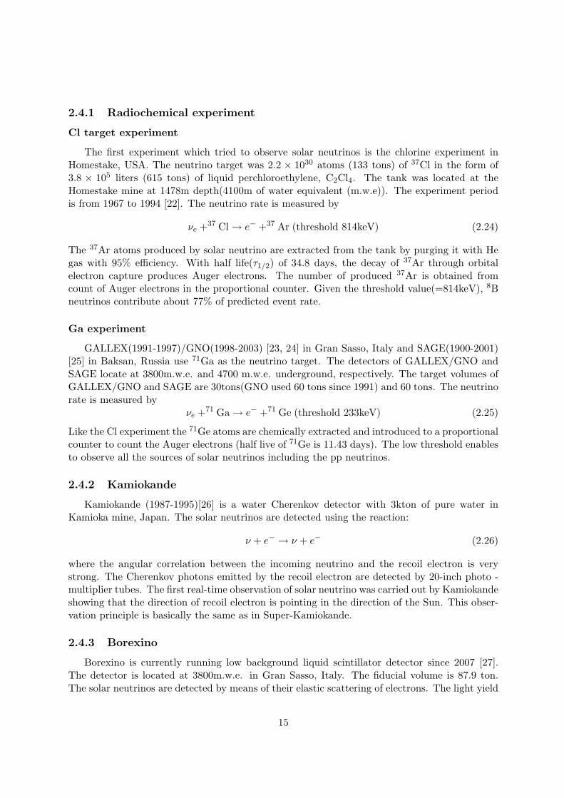
2.4.1 Radiochemical experiment
Cl target experiment
The first experiment which tried to observe solar neutrinos is the chlorine experiment inHomestake, USA. The neutrino target was 2.2 × 1030 atoms (133 tons) of 37Cl in the form of3.8 × 105 liters (615 tons) of liquid perchloroethylene, C2Cl4. The tank was located at theHomestake mine at 1478m depth(4100m of water equivalent (m.w.e)). The experiment periodis from 1967 to 1994 [22]. The neutrino rate is measured by
νe +37 Cl → e− +37 Ar (threshold 814keV) (2.24)
The 37Ar atoms produced by solar neutrino are extracted from the tank by purging it with Hegas with 95% efficiency. With half life(τ1/2) of 34.8 days, the decay of 37Ar through orbitalelectron capture produces Auger electrons. The number of produced 37Ar is obtained fromcount of Auger electrons in the proportional counter. Given the threshold value(=814keV), 8Bneutrinos contribute about 77% of predicted event rate.
Ga experiment
GALLEX(1991-1997)/GNO(1998-2003) [23, 24] in Gran Sasso, Italy and SAGE(1900-2001)[25] in Baksan, Russia use 71Ga as the neutrino target. The detectors of GALLEX/GNO andSAGE locate at 3800m.w.e. and 4700 m.w.e. underground, respectively. The target volumes ofGALLEX/GNO and SAGE are 30tons(GNO used 60 tons since 1991) and 60 tons. The neutrinorate is measured by
νe +71 Ga → e− +71 Ge (threshold 233keV) (2.25)
Like the Cl experiment the 71Ge atoms are chemically extracted and introduced to a proportionalcounter to count the Auger electrons (half live of 71Ge is 11.43 days). The low threshold enablesto observe all the sources of solar neutrinos including the pp neutrinos.
2.4.2 Kamiokande
Kamiokande (1987-1995)[26] is a water Cherenkov detector with 3kton of pure water inKamioka mine, Japan. The solar neutrinos are detected using the reaction:
ν + e− → ν + e− (2.26)
where the angular correlation between the incoming neutrino and the recoil electron is verystrong. The Cherenkov photons emitted by the recoil electron are detected by 20-inch photo -multiplier tubes. The first real-time observation of solar neutrino was carried out by Kamiokandeshowing that the direction of recoil electron is pointing in the direction of the Sun. This obser-vation principle is basically the same as in Super-Kamiokande.
2.4.3 Borexino
Borexino is currently running low background liquid scintillator detector since 2007 [27].The detector is located at 3800m.w.e. in Gran Sasso, Italy. The fiducial volume is 87.9 ton.The solar neutrinos are detected by means of their elastic scattering of electrons. The light yield
15

of the scintillator which is measured as 500 p.e./MeV enables the real-time detection of 7Beneutrinos, mainly. The neutrino rate can be obtained after statistical subtraction of radioactivebackground.
2.4.4 SNO
The Sudbury Neutrino Observatory (SNO, 1999-2006) [28, 29, 30] uses 1000 tons of D2Ocontained in a spherical vessel. The detector is located at 6010m.w.e. in Sudbury, Canada. SNOmearsures 8B neutrinos via the reactions
Charged Current(CC) : νe + d → p + p + e − 1.442MeV (2.27)Neutral Current(NC) : νx + d → p + n + νx − 2.224MeV (2.28)
Elastic Scattering(ES) : νx + e− → νx + e− (2.29)
where x = e, µ, τ . SNO has 3 phases of the experiment, and each phase has different methodof the neutron tagging. In Phase I, only pure D2O is contained, and the neutrons are capturedby D2O with the emission of 6.25MeV γ which is used to tag the NC event [28]. In Phase II,2tons of NaCl were added to enhance both the neutron capture efficiency and the total γ energy(8.6MeV) [29]. In Phase III, an array of 36 strings of proportional counters filled with 3He areinstalled to detect the neutrons [30]. Since CC is sensitive only to νe and NC is sensitive to alltypes of neutrinos, SNO can actually measure how many fraction of νe oscillate to νx by takingratio of CC rate to NC rate, which is the most significant result from SNO.
2.4.5 Summary of solar neutrino experimental results
Figure 2.9 summarize the results of solar neutrino experiment. The neutrino oscillation is nottaken into account for the SSM predictions in that figure. If the neutrino oscillation is considered,then the SSM and the experimental results agree very well as shown in Figure 2.10 In the Figures,the unit of SNU for Ga, Cl experiment stands for ”Solar Neutrino Unit” which is defined as 10−36
captures per target atom per second. To obtain the expectation flux with neutrino oscillation inFigure 2.10, the favored Large Mixing Angle (LMA) area (∆m2 = 6 × 10⁻⁵eV 2, tan2 θ12 = 0.4)is assumed.
2.5 Motivation and strategies of this thesis
The biggest remaining problem is to find the MSW effect in solar neutrinos. Figure 2.11shows the survival probability of νe as a function of neutrino energy. Super-Kamioande canobserve the energy spectrum in terms of the total electron energy which is deposited by a recoilelectron. Figure 2.12 shows the spectrum observed in the first phase of Super-Kamiokandeexperiment (SK-I) and predicted spectrum shapes with different oscillation parameters. Asshown in Figure 2.12, it is still difficult to decide whether the distorted spectrum is correct ornot because the sizes of the statistical uncertainty in lower energy region and the systematicuncertainty in higher energy region are large. Likewise, no other experiment has observed thedistorted spectrum successfully. Therefore, the final goal of this thesis is to observe the distortedspectrum. The following improvements are necessary to observe the spectrum distortion as soonas possible.
16

Figure 2.9: Comparison between various experimental results and SSM. The neutrino oscillationis not taken into account.
Figure 2.10: Comparison between various experimental results and SSM. The neutrino oscillationis taken into account.
17

ν
ν
θ
∆
Figure 2.11: Survival probability of electron neutrino with the solar best fit 2 flavor oscillationparameters.
Figure 2.12: Observed energy spectrum/SSM. The color histograms show expected value fordifferent oscillation parameters, and the gray band shows the energy correlated systematic un-certainty.
18

Figure 2.13: Expected energy spectrum after 5 years observation. The black histogram showsthe expect value with expected statistical uncertainty with 70% background reduction below 5.5MeV region. The blue band shows half size of energy correlated uncertainty as SK-I.
First, the number of background must be reduced to make the statistical uncertainty smallerespecially in the lower energy region (<5.5MeV). This is because the size of statistical uncertaintyis approximately the size of the square root of (statistical uncertainty of background)2 plus(statistical uncertainty of signal)2 and the statistical uncertainty of background is dominant forthe low-energy region. The numerical goal is to reduce 70% of background from SK-I level inthe lower-energy region. It was known from radioactive measurement of detector water that40% of remaining low energy background around 5MeV was due to radioactive impurities in thewater during SK-I, thus 40% reduction was expected because the water purification system andcirculation system had been upgraded since SK-I. The other 60% of background was consideredto be miss-reconstructed events which originally occurred in the edge of the detector but werereconstructed inside the fiducial volume. Such miss-reconstructed events could be reduced byhalf if new reconstruction tools and reduction tools are developed.
Second, the energy correlated systematic uncertainty must be reduced by 50% comparedto SK-I. To reduce the systematic uncertainty, the most important thing is to understand thedetector response. Thus, careful calibrations and tuning of the detector simulation are key tomake the reduction possible. Another strategy is to update the theoretical calculation of 8Bspectrum as already discussed in Section 2.2.
Figure 2.13 shows predicted energy spectrum after 5 years observation with reduced back-ground and systematic uncertainty. By comparing with Figure 2.12, we can see the upturn ofthe distorted spectrum with the reduced size of uncertainties. In this thesis, because the totallivetime is about one third of SK-I, it is difficult to confirm the upturn statistically, however,these improvements which will be discussed in the following chapters must set the foundationfor the future observation of the MSW effect in the Sun.
19

Chapter 3
Super-Kamiokande Detector
3.1 Detector outline
Super-Kamiokande is a cylindrical water Cherenkov detector with 50kton of ultra-pure water.The diameter of the detector is 39.3m, and the height is 41.4m. The detector location is 1000munderground (2700 m.w.e.) in the Kamioka mine, Gifu Pref., Japan, The latitude and longitudeare 36◦25’ N and 137◦18’ E, respectively. The downward-going cosmic-ray muon rate is about2Hz which is 10−5 times smaller than that at the ground level. The outside 2m of the detector iscalled the Outer Detector (OD) corresponding 18kton of volume, and the inside 32kton is calledthe Inner Detector (ID). ID and OD are separated by plastic black sheet and stainless steelstructure on which ID and OD photo-multiplier tubes (PMTs) are assembled. The purpose ofOD is to veto events from outside rock and reject cosmic-ray muon events. The fiducial volumeis 22.5kton, 2m inside from the ID wall.
Figure 3.1 is a brief description of the detector in each phase of the experiment. As shownin the figure, SK has three phases of the experiment which are called SK-I, II, and III1 Afterthe full reconstruction in 2006, 11129 20-inch PMTs in ID, and 1885 8-inch PMTs in OD areinstalled. The photodetector coverage is 40% in ID. The detail information about the detectorcan be found in [31].
The update items from SK-I(or II) are
• ID PMTs are covered by FRP and acrylic case.
• Water purification system is upgraded (see the section 3.4)
• Detector calibration is improved.
• OD is segmented by Tyvek which improved the Cosmic-ray muon identification (see Figure3.9).
3.2 20-inch PMT
R3600-06 HAMAMATSU PMT are used for ID PMT. Figure 3.2 shows a schematic view ofa 20-inch PMT and the bleeder circuit. In Figure 3.3, the basic specifications of those PMTsare listed. Figure 3.4 shows basic distributions measured by HAMAMATSU [32].
1SK-IV has started since Sep.6 2008 with new electronics and DAQ system.
20

Figure 3.1: Time-line of each phase of Super-Kamioande experiment.
2
Figure 3.5 shows the transparency of the acrylic cover for photons with normal incidencein water. The transparency is more than 96% for longer wavelength than 350nm, which isreasonably good considering the quantum efficiency of 20-inch PMT (see Figure 3.4).
3.3 Data acquisition (DAQ) system
Figure 3.6 shows a schematic view of the DAQ system. The signal from each ID PMT is sentto each channel of front-end electronics called Analog Timing Module (ATM) [33, 34] througha 70m coaxial cable. The ATM is developed based on the TKO standard [35]. 12 PMTs areconnected to one ATM, which records and digitizes the integrated charge and the arrival timinginformation with a 12-bit ADC. Each ATM channel has 2 buffer channels (a and b) to processsuccessive events, such as a muon and the decay electron after the muon. Thus, one ATM has24 channels (0a to 11b). The ATM characteristics is summarized in Table 3.1
The analog input of the ATM is made following the block giagram which is shown in Figure3.7. If a hit exceed a threshold (0.25p.e.), the signal charge is integrated at Charge to AnalogConverter (QAC) with a 400 nsec gate, and Time to Analog Converter (TAC) starts to integratecharge with a constant current to measure the time interval between the start time generated by
2Radiant sensitivity is the photoelectric current from the photocathode, divided by the incident radiant powerat a given wavelength, expressed in A/W (amperes per watt). Quantum efficiency (QE) is the number of pho-toelectrons emitted from the photocathode divided by the number of incident photons. Quantum efficiency isusually expressed as a percent. Quantum efficiency and radiant sensitivity have the following relationship at agiven wavelength.
21

Figure 3.2: Schematic veiw of the 20-inch PMT and the bleeder circuit [32].
Number of channels 12 ch/board
One hit processing time ∼ 5.5µsec
Charge dynamic range ∼ 400 to 600pC (12bit)
Timing dynamic range ∼ 1300nsec (12bit)
Charge resolution (LSB) 0.2 pC/LSB
Charge resolution (RMS) 0.2 pC (RMS)
Timing resolution (LSB) 0.3 ∼ 0.4nsec/LSB
Timing resolution (RMS) 0.4 nsec (RMS)
Temperature dependence (QAC) 3 Count/deg. ↔ 0.6 pC/deg.
Temperature dependence (TAC) 2 Count/deg. ↔ 0.8 nsec/deg.
Envent number 8 bit
Data size of one hit 6 Byte
FIFO 2 kByte (∼ 340 hits)
Table 3.1: Specifications of the ATM module
22

Figure 3.3: Specifications of the 20-inch PMT [32]
Figure 3.4: Basic distributions of 20-inch PMT (a) Cathode radiant sensitivity and Quantumefficiency. (b) 1p.e. charge distribution (c) Transit time distribution [32]
23

Figure 3.5: Transparency of acrylic cover as a function of the photon wavelength.
the hit signal and the stop signal which will be generated by a global trigger. After the globaltrigger arrived, the integrated charge in QAC and TAC are digitized in ADC. (Note that theoutput of a hit timing is the time interval between the hit and the global trigger, and thus, thebigger value of the output timing corresponds to earlier hit.) On the other hand, if there is noglobal trigger within 1.3µsec, the charges in QAC and TAC are cleared.
Every 16 events, the digitized data in the ATM are sent to VME memory module calledSuper Memory Partner (SMP). One SMP handle 20 ATMs and there are 8 slave computers eachreading out 6 SMP memories. One sequence of data flow ends with the online host computer towhich the slave computer sends its data.
More detailed information about the DAQ system is described in [31].
Trigger
The global trigger is made in the following process. At each ATM, in parallel with theprocesses in QAC and TAC, a hit signal is converted to a square pulse, then the ATM generateone HITSUM signal of 200nsec width by taking analog-sum of all the square pulses from 12PMTs. The height of the summed HITSUM is proportional to the number of hit PMTs in theATM. All HITSUMs are collected and AC-coupled into a discriminator to subtract offset due todark noise hits. At this point, one hit corresponds to -11mV of the pulse height. If the summedHITSUM signal exceed a discriminator threshold, a global trigger is generated and then it fedto a VME TRiGger module (TRG) which issues the global trigger and the event number to bedistributed to ATMs.
There are three types of the threshold values depending on the analysis region: Super LowEnergy trigger (SLE), Low Energy trigger (LE), and High Energy trigger (HE). Table 3.2 showsthe summary of each trigger setting. There also exists OD trigger, which has similar to that ofID and independent of the ID system. The OD trigger threshold is set to 19 OD hits in 200nsec.
Since most of the SLE triggered events are caused by gamma-rays from the surroundingrock, and radioactive decay in the PMT and FRP, the vertex positions of such low energy
24

20-inch PMT
ATM
x 240
x 20
ATM
GONG
SCH
interface
SMP
SMP
SMP
SMP
SMP
SMP
TRIGGER
HIT INFORMATION
x 6
Analog Timing Module
Sparc
VME
online CPU(slave)
online CPU(slave)
online CPU(slave)
online CPU(slave)
online CPU(slave)
online CPU(slave)
online CPU(slave)
Sparc
VME
online CPU(slave)
Analog Timing Module
TKO
TKO
Sparc
Sparc
Sparc
Sparc
Sparc
Sparc
Sparc
Sparc
interface
online CPU(host)
online CPU
(slave)
VME
TRIGGER
Super Memory Partner
Super Memory Partner
SMP x 48 online CPU(slave) x 17
PROCESSOR
TRG
interrupt reg.
20-inch PMT
ATM
x 240
x 20
ATM
GONG
SCH
20-inch PMT
ATM
x 240
x 20
ATM
GONG
SCH
20-inch PMT
ATM
x 240
x 20
ATM
GONG
SCH
interface
SMP
SMP
SMP
SMP
SMP
SMP
PMT x 11129 ATM x ~1000
x 15
8ch x15 x8 =960ch
8ch(12x8=96PMT)/board
Analog sum of 12PMT signals
online CPU(slave)
Sparc
Fast Ethernet
Fa
st Eth
ern
et
Fa
st Eth
ern
et
FADC x 120
(HITSUM)
Figure 3.6: Schematic view of DAQ system
25

DISCRI.
THRESHOLD
PMT INPUT
DELAY
CU
RR
EN
TS
PL
ITT
ER
&
AM
PL
IFIE
R
PED_START
TRIGGER
to PMTSUM
to HITSUMW:200nsHITOUT
SELF GATE
START/STOP
TAC-A
QAC-A
TAC-B
QAC-B
CLEAR
CLEAR
GATE
GATE
QAC-B
TAC-B
QAC-A
TAC-A
to ADC
HIT
START/STOP
W:900ns
ONE-SHOT
GATE
Figure 3.7: Block diagram of ATM.
Trig. Type Thre. (mV) Hits Trg. Rate (Hz)
SLE1 -212 19 ∼ 1.3k
SLE2 -186 17 ∼ 3.5k
LE -302 27 ∼ 30
HE -320 29 ∼ 10
Table 3.2: Summary of trigger settings in SK-III. SLE1 and SLE2 are set in different periods.SLE1 is from Jan 2007 to Apr 2008, and SLE2 is from Apr 2008 to Aug 2008. LE and HE areused in whole SK-III period. See also Table 7.1. Hits shows corresponding number of hits atthe threshold value namely Hits = (Thre. mV)/(-11 mV). About 6 hits correspond to 1MeV ofthe electron energy.
26

Figure 3.8: Upgraded water purification system.
background events are concentrated in the edge of ID. To reduce the number of events to bestored, a fast vertex fitter, which is a realtime vertex fitter and is applied to only SLE triggeredevents, was installed to cut events outside the 22.5kton fiducial volume. This software filteringand associated online computer hardware are called the Intelligent Trigger (IT) [20].
3.4 Water purification system
The purified water in the detector is constantly circulated through the water purificationsystem with a flow rate of 60 ton/hour. Figure 3.8 shows the upgraded water purificationsystem. Reverse Osmosis fiters (RO) remove particles, and RO3-a was installed during SK-I after supplying water, but it was used from the begining of SK-III, and a new RO3-b wasinstalled during SK-III. In addition, a new heat exchanger was installed, so that the watertemperature can be controlled with 0.1◦C accuracy. A brief description of the purificationsystem components is summarized in Table 3.3.
Figure 3.9 shows the circulation mode before and after the improvements of the system inSK-III. This final setting has been running since August, 2007. Before the improvements, wetested many circulation modes to achieve a stable and low background rate. It accidentallyhappened that sometimes radon-rich water contaminates even deep inside the fiducial volume.Such high background periods are eliminated from the final data sample for the very low energyregion from 4.5MeV to 6.5MeV. (see Section 7.1).
27
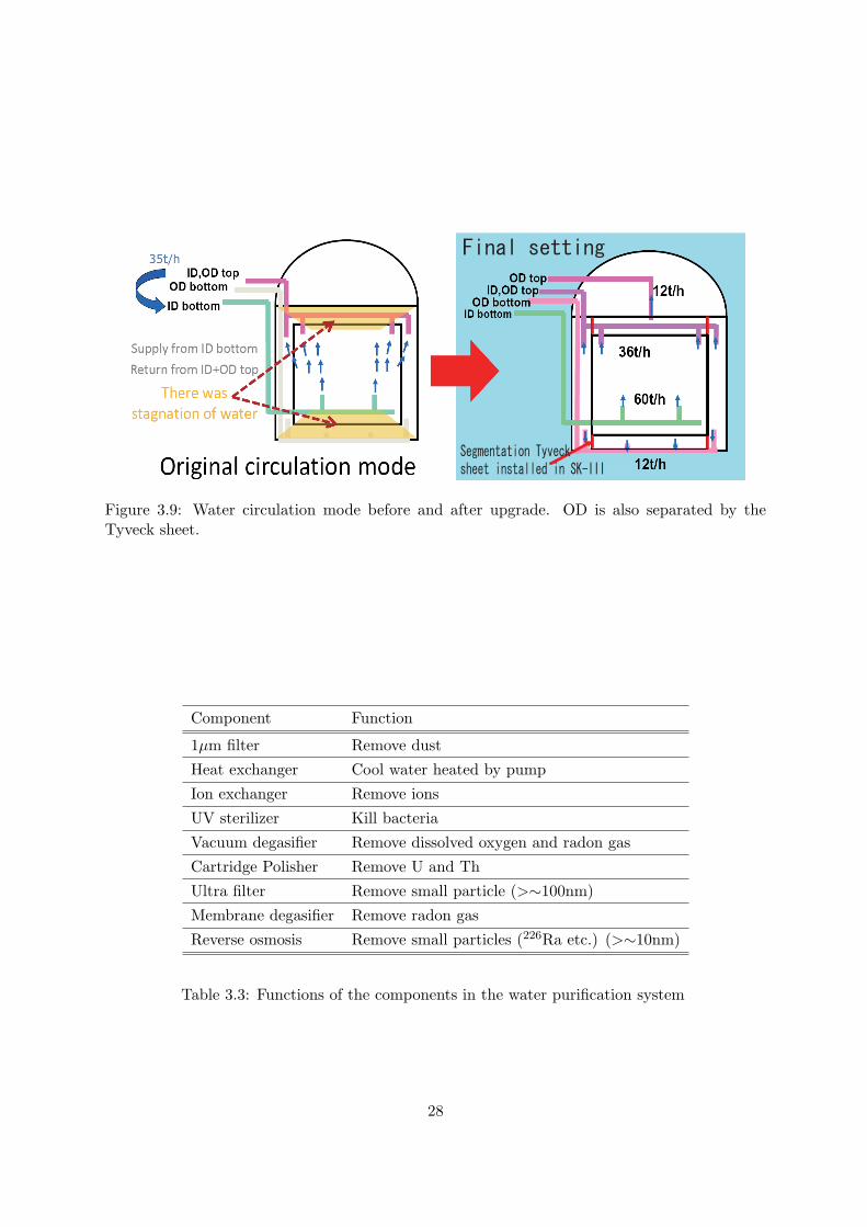
Figure 3.9: Water circulation mode before and after upgrade. OD is also separated by theTyveck sheet.
Component Function
1µm filter Remove dust
Heat exchanger Cool water heated by pump
Ion exchanger Remove ions
UV sterilizer Kill bacteria
Vacuum degasifier Remove dissolved oxygen and radon gas
Cartridge Polisher Remove U and Th
Ultra filter Remove small particle (>∼100nm)
Membrane degasifier Remove radon gas
Reverse osmosis Remove small particles (226Ra etc.) (>∼10nm)
Table 3.3: Functions of the components in the water purification system
28

After the improvements, the background level in the central region of the fiducial volumebecome significantly lower . This will be discussed in Chapter 10.
29

Chapter 4
Event reconstruction
The event reconstruction for solar neutrino events will be explained in this chapter. Super-Kamiokande observes the solar neutrino by detecting Cherenckov photons emitted from therecoil electron of the ν − e elastic scattering:
ν + e− −→ ν + e− (4.1)
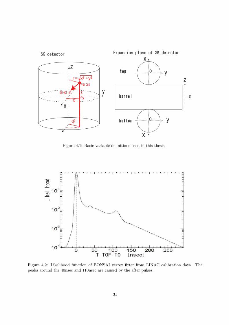
Since the recoil electron from a solar neutrino can travel only ≤∼10cm in water, it can beassumed that the Cherenkov photons are emitted from point-like source. First item is vertexreconstruction which finds the interaction point. After the vertex reconstruction, the directionand energy of recoil electron are reconstructed. Figure 4.1 explains the basic variables in theSK detector.
4.1 Vertex reconstruction
The event vertex reconstruction for solar neutrino analysis performs a maximum likelihoodfit to the timing residuals of the Cherenkov signal as well as the dark noise background for eachtesting vertex. This vertex fitter is called BONSAI [36]. The definition of the likelihood is
L(x⃗, t0) =Nhit∑i=1
log(P (t − tof(x⃗) − t0)) (4.2)
Here, x⃗ and t0 are the testing vertex position and the peak of hit timing t subtracted by Time OfFlight(tof) from the testing vertex x⃗ to each PMT position. Nhit is the number of hit PMTs,and P is a probability density function (pdf) which describes timing distribution of a signalevent as a function of the hit timing. The pdf is obtained from the shape of the timing residual(t− tof − t0) distribution from LINAC calibration data which is shown in Figure 4.2, and PMTdark noise is taken into account by constructing the likelihood.
The testing vertex with the largest likelihood is chosen as the reconstructed vertex. However,the accidental coincidence of dark noise hits after time-of-flight subtraction could produce localmaxima of the likelihood at several positions which are far away from the true vertex. Thesearch for the true global maximum is complicated and time consuming due to the large volumeof the detector. To improve both the speed performance and the number of mis-reconstructions,the likelihood is then maximized from a vertex search from a list of vertex candidates calculated
30
0
0
0
ϕ
Figure 4.1: Basic variable definitions used in this thesis.
Figure 4.2: Likelihood function of BONSAI vertex fitter from LINAC calibration data. Thepeaks around the 40nsec and 110nsec are caused by the after pulses.
31
from PMT hit combinations of 4 hits each. The four-hit combinations each define a uniquevertex candidate given their timing constraints. Thus, any events with four hits or more isreconstructed. The likelihood values for each vertex candidate are then calculated. To avoid alocal maximum point, iterations of grid search (from 7.8m to 1cm)around each candidate aredone until it finds a vertex which gives lager and more stable likelihood values at the surroundinggrid points. We also use the result from the second vertex fitter which is described in [20] as across check and a noise reduction.
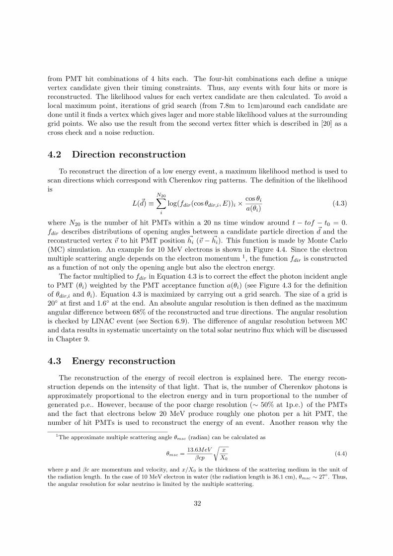
4.2 Direction reconstruction
To reconstruct the direction of a low energy event, a maximum likelihood method is used toscan directions which correspond with Cherenkov ring patterns. The definition of the likelihoodis
L(d⃗) ≡N20∑
i
log(fdir(cos θdir,i, E))i ×cos θi
a(θi)(4.3)
where N20 is the number of hit PMTs within a 20 ns time window around t − tof − t0 = 0.fdir describes distributions of opening angles between a candidate particle direction d⃗ and thereconstructed vertex v⃗ to hit PMT position h⃗i (v⃗ − h⃗i). This function is made by Monte Carlo(MC) simulation. An example for 10 MeV electrons is shown in Figure 4.4. Since the electronmultiple scattering angle depends on the electron momentum 1, the function fdir is constructedas a function of not only the opening angle but also the electron energy.
The factor multiplied to fdir in Equation 4.3 is to correct the effect the photon incident angleto PMT (θi) weighted by the PMT acceptance function a(θi) (see Figure 4.3 for the definitionof θdir,i and θi). Equation 4.3 is maximized by carrying out a grid search. The size of a grid is20◦ at first and 1.6◦ at the end. An absolute angular resolution is then defined as the maximumangular difference between 68% of the reconstructed and true directions. The angular resolutionis checked by LINAC event (see Section 6.9). The difference of angular resolution between MCand data results in systematic uncertainty on the total solar neutrino flux which will be discussedin Chapter 9.
4.3 Energy reconstruction
The reconstruction of the energy of recoil electron is explained here. The energy recon-struction depends on the intensity of that light. That is, the number of Cherenkov photons isapproximately proportional to the electron energy and in turn proportional to the number ofgenerated p.e.. However, because of the poor charge resolution (∼ 50% at 1p.e.) of the PMTsand the fact that electrons below 20 MeV produce roughly one photon per a hit PMT, thenumber of hit PMTs is used to reconstruct the energy of an event. Another reason why the
1The approximate multiple scattering angle θmsc (radian) can be calculated as
θmsc =13.6MeV
βcp
√x
X0(4.4)
where p and βc are momentum and velocity, and x/X0 is the thickness of the scattering medium in the unit ofthe radiation length. In the case of 10 MeV electron in water (the radiation length is 36.1 cm), θmsc ∼ 27◦. Thus,the angular resolution for solar neutrino is limited by the multiple scattering.
32

SK detectorν
θi
θdir,i
Figure 4.3: Definition of θdir,i and θi.
Figure 4.4: Angular likelihood of 10 MeVelectron
θ
Figure 4.5: Likelihood of angular reconstruc-tion depending on energy.
33

number of hits is used for energy calculation is that the number of hits does not strongly dependon the gain of PMTs compared to the total p.e.
N50 is defined as the maximum number of hits found by 50nsec sliding time window searchof T − Tof − T0 distribution. Since N50 is affected by several factors, such as accidental hitsfrom dark noise of PMTs, the effective number of hits (Neff ) is used to estimate the energy ofan event. The definition of Neff is following;
Neff =N50∑
i
{(Xi + ϵtail − ϵdark) ×
Nall
Nalive× 1
S(θi, ϕi)× exp(
ri
λ(run)) × Gi(t)
}(4.5)
where the explanation of each correction are following;
Xi: Multi-photo-electron hit correction
This correction is needed to estimate the effect of multiple photo-electrons in the i-th hitPMT due to the fact that if an event occurs close to a detector wall and is directed towardsthe same wall, the Cherenkov cone does not have much distance to expand then the observednumber of hits becomes smaller. The correction Xi is defined as
Xi =
log 1
1−xixi
, xi < 13.0, xi = 1
(4.6)
where xi is the ratio of hit PMTs in a 3×3 PMTs surrounding the i-th PMT to the total numberof live PMTs in the same area. The − log(1−xi) term is then the estimated number of photonsper one PMT in that area and is determined from Poisson statistics. When xi = 1, 3.0 isassigned to the value.
edark: Correction for dark noise hits
This factor is for hits due to dark noise in the PMTs.
ϵdark =50nsec × Nalive × Rdark
N50(4.7)
where Nalive is the number of all live ID PMTs and Rdark is the measured dark rate for a givenrun.
etail: Correction for late hit
Some Cherenkov photons being scattered for reflected arrive late to the PMT, and make latehit outside the 50nsec time window. To correct the effect of the late hits, the term
ϵtail =N100 − N50 − Nalive × Rdark × 50nsec
N50(4.8)
is added where N100 is the maximum number of hits found by 100nsec sliding time windowsearch.
34

Figure 4.6: Correction factor of photocathode coverage.
NallNalive
: Dead PMT correction
This factor is for the time variation of the number of dead PMTs. Nall is total number ofPMTs in SK-III and is 11129.
1S(θi,ϕi)
: Correction for photo-cathode coverage
This term is to account for the direction-dependent photcathode coverage. S(θi, ϕi) is theeffective photocathode area of the i-th hit PMT as viewed from the angles (θi, ϕi) which is shownin Figure 4.6. The definition of (θi, ϕi) is shown in Figure 4.7.
exp( riλ(run)):Water transparency correction
The water transparency is accounted for by this factor where ri is the distance from thereconstructed vertex to the i-th hit PMT. λ(run) is the measured water transparency for agiven run.
Gi(t): PMT gain correction
This factor is to adjust the relative gain of the PMTs at the single photo-electron level. Thedifferences in gain depend on the fabrication date of the PMTs.
After determining Neff , an event’s energy in terms of MeV can be calculated as a functionof Neff . The relation between Neff and MeV is obtained by uniform electron MC events , andthe systematic uncertainty of the reconstructed energy is checked by LINAC and DT calibration(see Section 6.7.2)
35

Figure 4.7: Definition of (θi, ϕi).
36

Chapter 5
Simulation
5.1 Outline of detector simulation
The detector response can be understood by Monte Carlo(MC) simulation of the detector. Insolar neutrino event simulation, the tracking of the recoil electron and the emission of Cherenkovphotons are done in the first step. In the second step, the Cherenkov photons are propagated.Finally, the response of the detector is simulated. Most of the physics processes such as multiplescattering or bremsstrahlung are simulated by GEANT3.21 [37], except for the production andthe propagation of Cherenkov photons and the light attenuation in water, which are developedby SK group [38].
Cherenkov photon production
The number of Cherenkov photons dN emitted by an electron per wavelength interval dλper track length dx is given by
dN = 2πα
(1 − 1
n2β2
)1λ2
dxdλ (5.1)
where n is the refractive index of water (n = 1.334), α is the fine structure constant, and βis the velocity of the electron in unit of the light velocity in vacuum. The opening angle θ ofCherenkov photons is given by
cos θ =1
nβ(5.2)
Based on these formulae, Cherenkov photons are produced in the simulation.
Propagation of photons in water
The velocity of Cherenkov photons depends on its wavelength. The velocity is given as agroup velocity (vg) of the wave packet:
vg =c
n(λ) − λdn(λ)dλ
(5.3)
where n(λ) is the refractive index of water as a function of the wavelength such as
n(λ) =√
a1
λ2 − λ2a
+ a2 + a3λ2 + a4λ3 + a5λ6. (5.4)
37

The unit of λ is µm, and parameters are
λ2a = 0.018085, a1 = 5.7473534 × 10⁻³
a2 = 1.769238, a3 = −2.797222 × 10⁻²
a4 = 8.715348 × 10⁻³, a5 = −1.413942 × 10⁻³
These are obtained by measurements.There are three processes which are considered during the photon propagation: Rayleigh
scattering, Mie scattering, and absorption. The attenuation length (Lattn.) of light in water isthen given by
Lattn. =1
αabs(λ) + αRayleigh(λ) + αMie(λ)(5.5)
where αabs(λ), αRayleigh(λ), αMie(λ) are coefficients for the absorption, Rayleigh scattering, andMie scattering as a function of the wavelength of photons (λ). The fraction of these processesdepends on the wavelength and the purity of water. The wavelength dependence of each processis given by
αabs(λ) =
A1λ4 , λ ≤ 350nmA1λ4 + A2(λ/A3)A4 , 350 < λ ≤ 415nmA1λ4 + f(λ), 415nm < λ
(5.6)
αRayleigh(λ) =R1
λ4× (1 +
R2
λ2) (5.7)
αMie(λ) =M1
λ4(5.8)
where Ax, Rx,Mx are tuning parameters, and f(λ) is measured by [39]. The measurement isdone by a periodical laser injection calibration. When a photon arrives at the detector wall (theacrylic cover, the PMT surface or the black sheet), the reflection, absorption and transmissionare considered. An example of the fraction of these processes at the PMT surface is shown inFigure 5.1.
Detector response
When a photon reaches at the PMT surface, the detector response is simulated. The proba-bility to produce one p.e. from the photon arriving at each PMT surface has four components:
Probability = QE(λ) × AorP (λ, θi)AorP (λ, 0)
× COREPMT × qetable(i) (5.9)
where QE(λ) is the quantum efficiency of 20-inch PMT depending on the wavelength of theincident photon λ, which is measured by HAMAMATSU, AorP (λ, θ) is summed fraction of theabsorption and p.e production (black + green in figure 5.1), and is measured by a calibrationwith injected laser light. Thus, AorP (λ,θi)
AorP (λ,0) is a correction depending on the incident angle θi
for the photon with λ. COREPMT corrects the average quantum efficiency (Q.E.) which iscommon to all PMTs and tuned by LINAC (see Section 6.6.2). Finally, qetable(i) is the relativeQ.E. for the i-th PMT measured by Ni calibration (see Section 6.1). After one p.e. is producedwith the probability, the output charge from PMT is simulated according to the measured 1
38
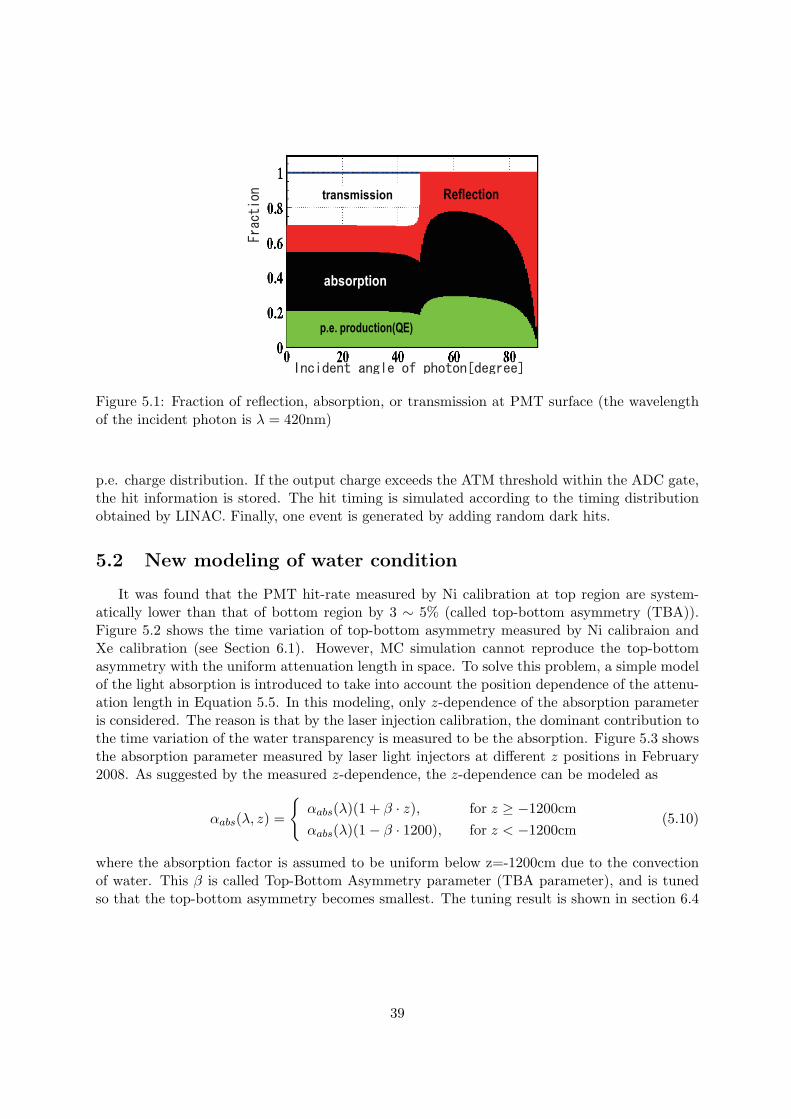
transmission
absorption
p.e. production(QE)
Reflection
Figure 5.1: Fraction of reflection, absorption, or transmission at PMT surface (the wavelengthof the incident photon is λ = 420nm)
p.e. charge distribution. If the output charge exceeds the ATM threshold within the ADC gate,the hit information is stored. The hit timing is simulated according to the timing distributionobtained by LINAC. Finally, one event is generated by adding random dark hits.
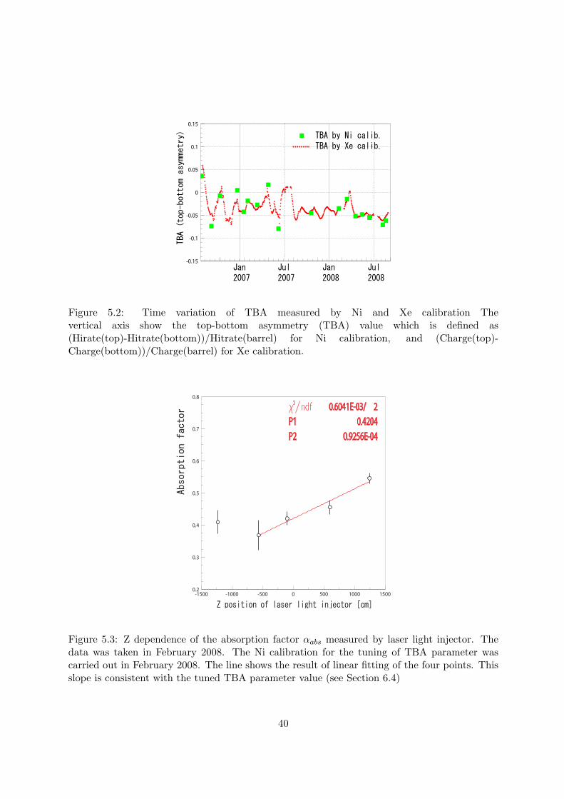
5.2 New modeling of water condition
It was found that the PMT hit-rate measured by Ni calibration at top region are system-atically lower than that of bottom region by 3 ∼ 5% (called top-bottom asymmetry (TBA)).Figure 5.2 shows the time variation of top-bottom asymmetry measured by Ni calibraion andXe calibration (see Section 6.1). However, MC simulation cannot reproduce the top-bottomasymmetry with the uniform attenuation length in space. To solve this problem, a simple modelof the light absorption is introduced to take into account the position dependence of the attenu-ation length in Equation 5.5. In this modeling, only z-dependence of the absorption parameteris considered. The reason is that by the laser injection calibration, the dominant contribution tothe time variation of the water transparency is measured to be the absorption. Figure 5.3 showsthe absorption parameter measured by laser light injectors at different z positions in February2008. As suggested by the measured z-dependence, the z-dependence can be modeled as
αabs(λ, z) =
{αabs(λ)(1 + β · z), for z ≥ −1200cmαabs(λ)(1 − β · 1200), for z < −1200cm
(5.10)
where the absorption factor is assumed to be uniform below z=-1200cm due to the convectionof water. This β is called Top-Bottom Asymmetry parameter (TBA parameter), and is tunedso that the top-bottom asymmetry becomes smallest. The tuning result is shown in section 6.4
39
-0.15
-0.1
-0.05
0
0.05
0.1
0.15
Figure 5.2: Time variation of TBA measured by Ni and Xe calibration Thevertical axis show the top-bottom asymmetry (TBA) value which is defined as(Hirate(top)-Hitrate(bottom))/Hitrate(barrel) for Ni calibration, and (Charge(top)-Charge(bottom))/Charge(barrel) for Xe calibration.
0.2
0.3
0.4
0.5
0.6
0.7
0.8
-1500 -1000 -500 0 500 1000 1500
0.6041E-03/ 2
P1 0.4204
P2 0.9256E-04
Figure 5.3: Z dependence of the absorption factor αabs measured by laser light injector. Thedata was taken in February 2008. The Ni calibration for the tuning of TBA parameter wascarried out in February 2008. The line shows the result of linear fitting of the four points. Thisslope is consistent with the tuned TBA parameter value (see Section 6.4)
40

1/a�
enua
�on
leng
th (
1/m
)
Wavelength(nm)
Abs.+Sca�.
Absopr�on
Ray. sca�.
Mie sca�.
Figure 5.4: Tuned water parameters measured by laser injection calibrationMakers show the measured parameters and lines show the fitted functions.
5.3 Tunable input parameters
The tunable parameters for MC simulation are listed here. The tuning results are shown inChapter 6.
Water parameters
The absorption and scattering parameters are measured by laser light injected from top, bar-rel, and bottom. Figure 5.4 shows the measured water attenuation length and the contributionof the absorption, Rayleigh scattering, and Mie scattering as a function of photon wavelengthfor SK-III.
TBA parameter
TBA parameter is tuned so that the hit-rate of MC simulation reproduces that of calibrationdata taken by Ni calibration. The time variation of TBA parameter is also implemented byperiodical measurements of the top-bottom asymmetry factor.
Timing resolution of PMT
Timing resolution of PMT is calibrated by LINAC. The hit timing is smeared by the measuredtiming resolution in MC simulation.
After pulse
PMT hit timing has some characteristic peaks after the main peak (called after pulse). Apossible explanation of the cause of the after pulse is that if a photo-electron is back scattered atthe first dynode, it takes some time until it loses its velocity against the electric field then comesback to the first dynode, producing a delayed hit. The fraction of the after pulse is measuredby LINAC calibration. (see Section 6.6.2)
41

Average quantum efficiency (Q.E.) of PMT
While the relative Q.E. of each PMT is measured by the Ni calibration, the average Q.E. istuned so that the Neff of MC simulation reproduces LINAC data.
42
Chapter 6
Calibration
6.1 Outline of detector calibrations
An outline of the detector calibration will be given in this section. Some important calibra-tions for the solar neutrino measurement such as timing of PMT, water transparency, quantumefficiency(Q.E.) of PMT, and LINAC are explained in the subsequent sections. Especially, theimprovement to the timing calibration is newly achieved in this thesis. The detail explanationof the detector calibration is in [31].
First, High Voltage (HV) value which is applied to each PMT is adjusted in order to achievethe same Q.E.× gain value for all PMTs becomes same within ±1% accuracy. This HV de-termination was done by light emission of Xe lamp guided through optical fiber (hereafter Xecalibration). A scintillator ball at the end of the optical fiber absorbs the UV light and emitslight isotropically with a peak at 440nm wavelength.
After the HV determination, the conversion factor of ADC charge to p.e. is measured foreach PMT. The conversion factor is given by (average PMT gain)×(relative PMT gain). Theaverage PMT gain is obtained from an average 1 p.e. distribution of PMTs measured by Cf-Niγ-ray source (peak energy ∼9MeV, average number of hits is 50PMTs, hereafter Ni calibration).The obtained value of average gain is 2.243 pC/p.e.. The relative PMT gain for each PMT isobtained by calibration data using high and low intensity laser light (398nm). The laser lightwas put into the detector through optical fiber and diffuser ball. The relative PMT gain (Gi: idenotes PMT ID) is the ratio of the mean charge (Qi) in the high intensity data to the numberof hits (Hiti) at the low intensity data for each PMT; Gi = Qi/Hiti. This is because the Qi
is proportional to Q.E. × gain, and the Hiti is proportional to only Q.E., thus, only the gainfactor can be extracted by taking the ratio of Qi to Hiti.
The charge of each PMT hit is corrected by taking into account the ADC non-linearity. Thisnon-linearity is measured by obtaining deviation of measured p.e value from the expected p.e.value. The data for this calibration is taken by laser light source.
In parallel to these calibration related to the charge of each hit, timing calibration, watertransparency measurement, and Q.E. measurement were done. Then LINAC and DT (deuteriumand tritium neutron generator) calibration were done especially for the low-energy event analysis.In the following sections, the explanation about these calibrations which are closely related tothe solar neutrino analysis will be given.
43

6.2 Timing calibration
The timing of all PMTs must be calibrated so that the event vertices and directions arereconstructed accurately. To obtain correct timing, the followings must be considered; the lightintensity of each PMT, the length of cable between each PMT and electronics, and different rangeof hit timings. Different light intensity makes different triggered timing which is so called ”timewalk”. The time walk exists because larger charge hits exceed TDC discriminator thresholdearlier than those with less charge even though the hit PMT gets photons in the same timing.The timing calibration for SK-III consists of two measurements; one is to make a correctiontable for the time walk and cable length, and the other one is to make a correction function forhit timings in different time ranges. It should be mentioned that the former one is a main part oftiming calibration which is basically same as the one in the previous phase of experiments, butthe latter one is newly introduced in SK-III to decrease the systematic shift of the reconstructedvertex position.
Conventional timing calibration
This calibration is to correct the time walk of each PMT and the overall process time foreach PMT (cable length and electronics. etc.). The time walk and the overall process timecan be measured by putting a fast pulsing light source in the center of the detector. Figure 6.1shows a schematic view of the timing calibration system. First, a N2 laser pulse is divided in the
Figure 6.1: Schematic view of timing calibra-tion system
890
900
910
920
930
940
950
960
970
980
990
T [
ns]
Figure 6.2: Example of TQ distribution.Horizontal axis shows charge of each hit, andVertical axis shows hit timing without correc-tion.
laser module. One goes to a trigger PMT which makes an external trigger for timing calibration
44

event. The other goes to dye laser module to produce a dye laser pulse. The dye laser pulse(wavelength; 398±5nm(FWHM), pulse width 0.2nsec) then goes through variable filter whichis used to adjust the laser intensity. After traveling 70m optical fiber, the dye laser pulse isemitted in the detector from a diffuser ball.
The calibration data are taken by changing the intensity of the light from the diffuser ball.Using the variable filter, the light intensity can be adjusted from 0.0 p.e. level to high intensitylevel (250p.e.) which causes saturation of electronics. Figure 6.2 shows a typical relation betweentiming and charge. The vertical axis shows the hit timing without correction, and the larger valuecorresponds to earlier hit timing. This two dimensional histogram is called ”TQ distribution”.The purpose of this calibration is to fit the TQ distribution by a proper function. This functionis called ”TQmap”.
The TQmap is made for each channel (11129 PMTs × 2 ATM buffer channels). The methodto generate TQmap is following. In the first step, after making the timing distribution plot foreach channel, selection of laser hit is done by setting 100 nsec time-window around the peak ofthe timing distribution with TOF(time of flight from the diffuser ball to each PMT) ”added”.The ”+” sign for TOF means that before the timing correction the vertical axis corresponds totime interval between the hit and the global trigger (see the DAQ section 3.3). Since the smallervalue of vertical axis shows the later hit, TOF must be added to get the time when a pulse lightis emitted from the diffuser ball.
A selection is needed to remove pre-pulses which occur at around 50nsec before the mainpeak by a photon hitting the dynode of PMT, and after-pulses which occur at about 100 nsecafter the main peak by an electron back scattered at the first dynode. After the selection oflaser hits, for each of the 140 bins in charge (Qbin), the peak timing and the standard deviationof timing distribution is obtained by asymmetric Gaussian fitting which takes into account theeffect of the scattered or reflected hits. The bin width of each charge bin is defined as
∆Qbin ≡
{0.2 pC, for 1 ≤ Qbin ≤ 50 (0 pC ≤ Q ≤ 10 pC)
10Qbin50 − 10
Qbin−1
50 , for 51 ≤ Qbin ≤ 140 (10 pC ≤ Q ≤ 630.95 pC)(6.1)
Finally, the peak timings with respect to the charge is fitted by a seventh order polynomialfunction.
An improvement of SK-III method is following. In SK-I and II, instead of the peak value,the timing of each charge bin was determined from an average timing. The timing obtainedby the previous method, therefore, was affected by late scattered or reflected hits especially atsmall charge regions. 1 Since the amount of reflected hits are large in the edge of ID, such effectgives systematic timing shift depending on PMT positions. Figure 6.3 shows one example of thedifference between the two methods. As shown in Figure 6.3, the hit timing of the new methodis faster than that of the old method at small charge region, which means that the new methodis less affected by the late hits.
1In the previous method, to reduce the effect of timing of late hits, First, an average is obtained from theselected hits within 100nsec for each Qbin. Then, for each Qbin, a narrow timing window is set +2.0RMS-1.5RMSaround the average timing within the 100 nsec time-window. Finally, the timing of each Qbin is determined fromthe average timing in the narrow time window.
45

920
925
930
935
940
945
950
955
960
965
970
0 20 40 60 80 100 120
0 20 40 60 80 100 120
Figure 6.3: Example of comparison between the old and new methods of TQmap.
46

Figure 6.4: Setup for additional timing calibration
Additional timing calibration
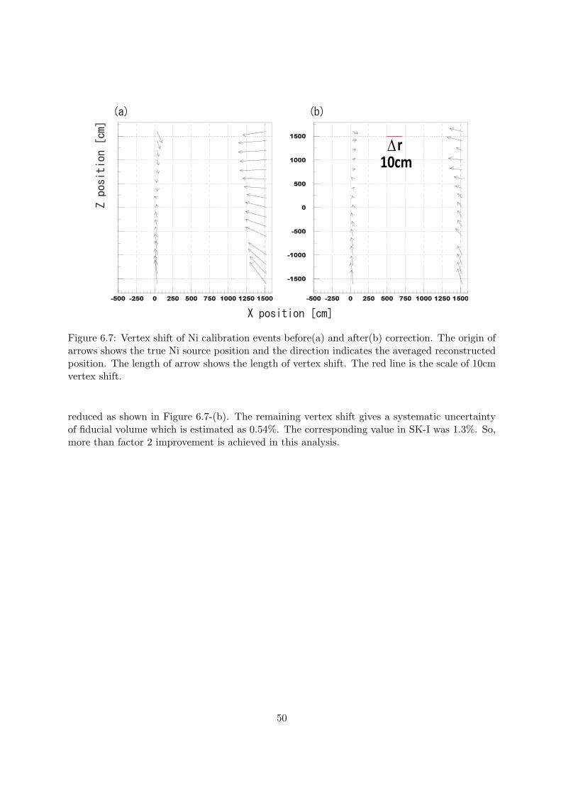
The other calibration which has been carried out is to improve the performance of recon-struction. It was observed that the reconstructed position of Ni calibration events was shiftedinward direction from the real source position to the tank center (see Figure 6.7-(a)).
This direction of the vertex shift indicates that the linearity of relative timing within a widerange (∼100nsec) is not perfect due to characteristics of electronics. For source positions awayfrom center and near the ID wall, the spread of hit times is larger (∼100nsec) if the TOF isnot subtracted. In this case, the earlier hits seem to be shifted later by ∼0.5nsec. This timingdifference between far side hits and near side hits can create the bias to reconstructed position.
I have measured this timing shift by the following setup. Figure 6.4 shows a schematicdiagram of trigger system of this calibration. In order to measure the timing shift betweenlate hit and early hit, a calibration trigger signal (common stop signal) from the monitor PMTis artificially delayed by putting additional cables (from 15m to 80m), and the time delay ismeasured by a independent system which is pre-calibrated within 0.1% accuracy. For example,a 20m cable can make the arrival time of the global trigger at each ATM by 50nsec later, whichcorresponds to make hit timing of each PMT 50nsec faster. By changing the cable length 15mup to 80m, we can check the relation of the timing measured by ATM and the timing measuredby the independent system within the range of about 300 nsec.
Figure 6.5 shows an example of the result for a PMT. The horizontal axis shows hit timemeasured by ATM, and vertical axis is delayed time measured by independent system. Whilethe horizontal axis and vertical axis show good linearity within ±1nsec as shown in the top plotof Figure 6.5, the difference has a clear dependence on the value of hit time. This tendencyis common to all channels which is shown in Figure 6.6. The average of fitted slope values is-0.67nsec/100nsec, thus correction function is
T = T − slope × (T − 1000.0) + offset(ch) (6.2)
where T is hit time, 1000.0nsec is selected as normalization point, and offset(ch) is an offsetvalue depending on ATM ch (0a ∼ 11b). After applying this correction, the vertex shift is
47

Figure 6.5: Example of timing shift as a function of hit timing range for one channel
48

Figure 6.6: timing shift as a function of absolute hit timing. Different colors show timing shiftof the different ATM channels (0a to 11b). The marker show mean timing shift of the sameATM channel PMTs with respect to the absolute hit timing. The lines show the results of linearfitting for all ATM channels.
49
10cm
∆r
Figure 6.7: Vertex shift of Ni calibration events before(a) and after(b) correction. The origin ofarrows shows the true Ni source position and the direction indicates the averaged reconstructedposition. The length of arrow shows the length of vertex shift. The red line is the scale of 10cmvertex shift.
reduced as shown in Figure 6.7-(b). The remaining vertex shift gives a systematic uncertaintyof fiducial volume which is estimated as 0.54%. The corresponding value in SK-I was 1.3%. So,more than factor 2 improvement is achieved in this analysis.
50

P1 1.424
P2 -0.8768E-04
0.8
0.9
1
1.1
1.2
1.3
1.4
1.5
1000 1500 2000 2500 3000 3500
Figure 6.8: Charge vs. distance from the decay-e vertex. Vertical is log of hit charge (p.e.) andline shows the result of linear fitting.
6.3 Water Transparency Measurement
The water transparency is measured by using decay electrons and positrons (hereafter decay-e) from cosmic-ray muons stopped in the detector (hereafter stopping µ). The selection criteriaof decay-e are following:
• The time difference between the stopping µ and the decay-e candidate (∆T ) must be2.0µsec < ∆T < 8.0µsec.
• The reconstructed vertex of the decay-e candidate must be within the 22.5-kton fiducialvolume (=2m from ID wall).
• The number of hit PMTs within 1.3µsec, Nhit ≥ 50
About 1500 decay-e events are selected with this criteria every day, which is statistically enoughfor this weekly transparency measurement.
Figure 6.8 shows the correlation between log of the charge (q(r)) of hit PMTs (vertical)and the distance from the decay-e vertex to each hit PMT (horizontal). The charge of PMT iscorrected considering the acceptance depending on the incident angle of photon. To eliminatescattered hits or reflected hits, hit PMTs are selected by the following criteria:
• Hit PMT must be one of N50.
• The opening angle of a hit PMT θdir must be 32◦ < θdir < 52◦
After fitting the histogram with linear function, the water transparency is obtained by the inverseof the fitted slope.
Figure 6.9 shows the time variation of the water transparency. Each point represent a watertransparency for 6 days.
51

6000
8000
10000
12000
14000
16000
07/01/06 10/01/06 01/01/07 04/01/07 07/01/07 10/01/07 01/01/08 04/01/08 07/01/08 10/01/08
Figure 6.9: Time variation of water transparency. Each point is determined from 6day dataperiod.
6.4 TBA tuning and Q.E. measurement by Ni calibration
As already described in the previous chapter, the TAB parameter is newly introduced to SK-III detector simulation to model the z-dependence of the absorption parameter. This parameteris tuned so that the PMT hit-rate of data and MC simulation shows the best agreement. Withthe tuned TBA parameter, the relative Q.E. of individual PMT is obtained by taking the ratioof the hit-rate of data to that of MC simulation. The usage of Ni-Cf γ-ray source is favoredbecause of following reasons
• Easy to operate and good isotropy.
• Low occupancy ( NhitTotal # of PMTs ∼ 1%) is needed to avoid multi-photon hit.
• Q.E. should be measured at the Cherenkov wavelength range.
Figure 6.10 shows a comparison of the hit-rate between data and MC simulation with TBA=0and TBA=tuned value respectively. Hit-rate is defined as number of hits in each PMT in a unitof the averaged number of hits for all PMT during the calibration run2. As shown by the figure,data and MC shows better agreement with TBA=tuned value (8.85×10⁻⁵). Then, the relativeQ.E. to be put into MC is obtained as the ratio of data to MC.
2The acceptance correction as a function of incident angle of photon to each PMT and the distance correctionbetween the source position and each PMT position are taken into account to obtain the number of hits for eachPMT.
52

Figure 6.10: Hit rate of data(Black) and MC simulation (Green: TBA=0,Red: TBA=tuned)
6.5 DT calibration
6.5.1 DT neutron generator
Deuterium-Tritium Generator [40] produce neutrons by colliding deuterium and tritium ionswith a fixed metal hydride target with a reaction;
3H +2 H −→ 4He + n (6.3)
The deuterium and tritium are ionized by Penning ion source. The energy of neutrons is 14.2MeVwhich is high enough to make 16N by the (n,p) reaction on 16O [41] in water. The 16N thendecays with a half-life of 7.13 second with gamma-ray and/or electrons. The dominant decaymode (66%)produces a 6.1MeV γ with an electron of 4.3MeV endpoint energy, while the seconddominant decay mode (28%) produce a 10.41MeV electron. The advantage of this calibration isfollowing; First, as shown in the Figure 6.11, this calibration is easier to operate compared toLINAC. Second, the data can be taken in many places. Third, the event direction is isotropic.Taking advantage of DT neutron generator, the data are uesd to study the uncertainty of energyscale depending on position and direction (see Section 6.7.2).
6.5.2 Trigger efficiency
In addition to data taking with the normal LE and SLE trigger threshold, special calibrationdata was taken with the threshold value at -150mV. With the special data, the trigger efficiencyis defined as follow ;
EffLE,j =NLE,j
Nspecial,j(6.4)
53

Figure 6.11: Schematic view of DT neutron generator calibration setup. (a) The generator isinserted in the tank, (b) Neutrons are created, (c) The generator is lifted 2 meters, so that wecan make the shadow effect of the the generator as small as possible.
EffSLE,j =NSLE,j
Nspecial,j(6.5)
where NLE(SLE),j is the number of events in j-th energy bin triggered by LE (SLE) threshold,and Nspecial,j is that of the special threshold. Figure 6.12 shows the trigger efficiency measuredby DT calibration compared with trigger simulation of MC. The difference between data andMC is 2.0% in 4.5-5MeV, 1.0% in 5-5.5MeV, 0.5% in 5.5-6MeV, and 0.1% in 6-6.5MeV (SLE2period). The trigger efficiency in higher energy region is 100%, thus the difference is negligible.
6.6 LINAC Calibration
6.6.1 the LINAC system
An introduction of the LINAC system will be given. The detail information can be found in[42]. Figure 6.13 and 6.14 show the schematic view of the LINAC system and structure of theend cap. The LINAC is a model ML-15MIII from Mitsubishi. During the operation, the beampipe is evacuated to less than 0.1Pa, and the beam size and momentum is tuned by collimatorand magnets. The energy range of the electron is selected from 4.4-18MeV, so that we can makea similar event as the recoil electron event. Other specifications are summarized in Table 6.1Due to the small systematic uncertainty of the system [42], we can use the LINAC data not onlyfor the absolute energy scale calibration but also for various systematic uncertainty studies.
54

0
0.2
0.4
0.6
0.8
1
1.2
2 3 4 5 6 7
Figure 6.12: An example of SLE trigger efficiency obtained by DT data and MC
Figure 6.13: The LINAC system Figure 6.14: The structure of end cap
55
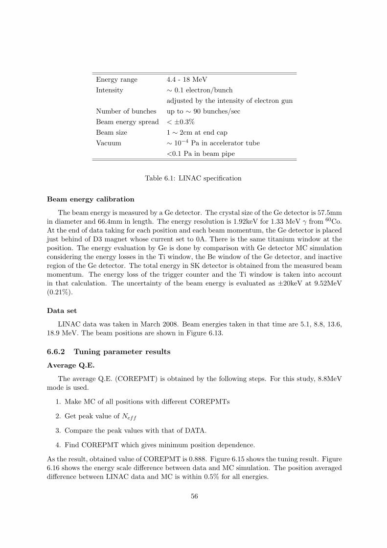
Energy range 4.4 - 18 MeVIntensity ∼ 0.1 electron/bunch
adjusted by the intensity of electron gunNumber of bunches up to ∼ 90 bunches/secBeam energy spread < ±0.3%Beam size 1 ∼ 2cm at end capVacuum ∼ 10−4 Pa in accelerator tube
<0.1 Pa in beam pipe
Table 6.1: LINAC specification
Beam energy calibration
The beam energy is measured by a Ge detector. The crystal size of the Ge detector is 57.5mmin diameter and 66.4mm in length. The energy resolution is 1.92keV for 1.33 MeV γ from 60Co.At the end of data taking for each position and each beam momentum, the Ge detector is placedjust behind of D3 magnet whose current set to 0A. There is the same titanium window at theposition. The energy evaluation by Ge is done by comparison with Ge detector MC simulationconsidering the energy losses in the Ti window, the Be window of the Ge detector, and inactiveregion of the Ge detector. The total energy in SK detector is obtained from the measured beammomentum. The energy loss of the trigger counter and the Ti window is taken into accountin that calculation. The uncertainty of the beam energy is evaluated as ±20keV at 9.52MeV(0.21%).
Data set
LINAC data was taken in March 2008. Beam energies taken in that time are 5.1, 8.8, 13.6,18.9 MeV. The beam positions are shown in Figure 6.13.
6.6.2 Tuning parameter results
Average Q.E.
The average Q.E. (COREPMT) is obtained by the following steps. For this study, 8.8MeVmode is used.
1. Make MC of all positions with different COREPMTs
2. Get peak value of Neff
3. Compare the peak values with that of DATA.
4. Find COREPMT which gives minimum position dependence.
As the result, obtained value of COREPMT is 0.888. Figure 6.15 shows the tuning result. Figure6.16 shows the energy scale difference between data and MC simulation. The position averageddifference between LINAC data and MC is within 0.5% for all energies.
56
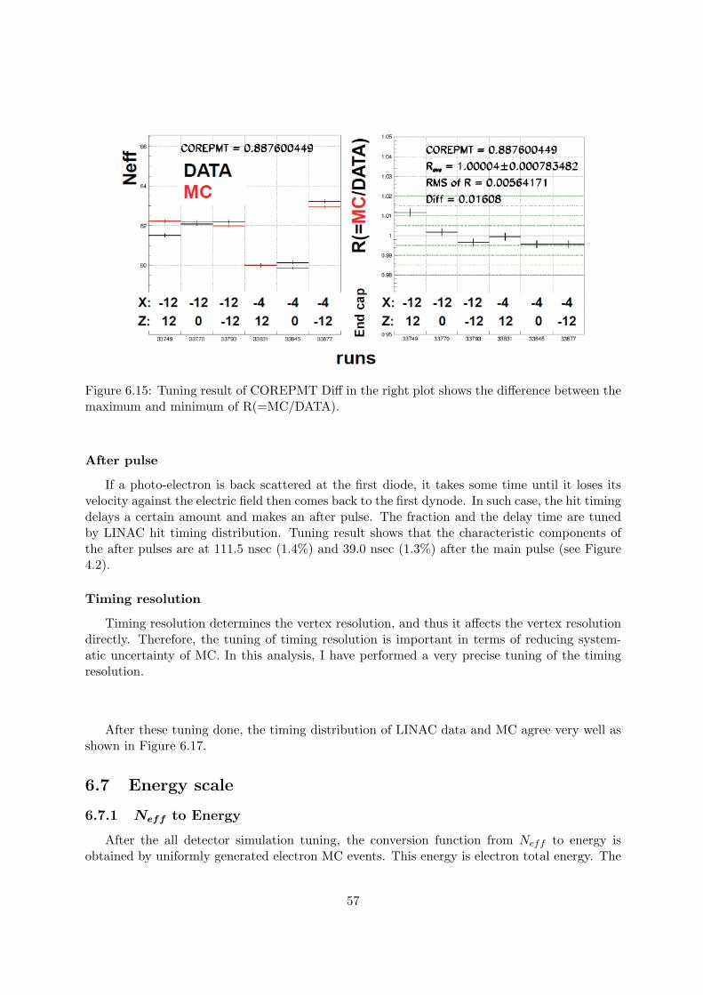
Figure 6.15: Tuning result of COREPMT Diff in the right plot shows the difference between themaximum and minimum of R(=MC/DATA).
After pulse
If a photo-electron is back scattered at the first diode, it takes some time until it loses itsvelocity against the electric field then comes back to the first dynode. In such case, the hit timingdelays a certain amount and makes an after pulse. The fraction and the delay time are tunedby LINAC hit timing distribution. Tuning result shows that the characteristic components ofthe after pulses are at 111.5 nsec (1.4%) and 39.0 nsec (1.3%) after the main pulse (see Figure4.2).
Timing resolution
Timing resolution determines the vertex resolution, and thus it affects the vertex resolutiondirectly. Therefore, the tuning of timing resolution is important in terms of reducing system-atic uncertainty of MC. In this analysis, I have performed a very precise tuning of the timingresolution.
After these tuning done, the timing distribution of LINAC data and MC agree very well asshown in Figure 6.17.
6.7 Energy scale
6.7.1 Neff to Energy
After the all detector simulation tuning, the conversion function from Neff to energy isobtained by uniformly generated electron MC events. This energy is electron total energy. The
57

20
40
60
80
100
120
140
4 6 8 10 12 14 16 18 20
Ne of DATA X = -1237cm, Z = 1197cm
X = -1237cm, Z = -6cmX = -1237cm, Z = -1209cmX = -388.9cm, Z = 1197cmX = -388.9cm, Z = -6cmX = -388.9cm, Z = -1209cm
20
40
60
80
100
120
140
4 6 8 10 12 14 16 18 20
Ne of MC
-0.05
-0.04
-0.03
-0.02
-0.01
0
0.01
0.02
0.03
0.04
0.05
4 6 8 10 12 14 16 18 20
(MC-DATA)/DATA
-0.05
-0.04
-0.03
-0.02
-0.01
0
0.01
0.02
0.03
0.04
0.05
4 6 8 10 12 14 16 18 20
expected energy in tank
(MC-DATA)/DATA
Figure 6.16: Energy scale difference of LINAC data and MC simulation . The left bottom plotshows the difference of each position (makers correspond to the position of Figure 6.13 ) Theright bottom plot shows the position averaged difference.
58

Figure 6.17: Timing distribution after tuning MC. LINAC 5.1MeV (x,z)=(-12m,12m)
relation between the energy and Neff is given
E = p1 + (p2 + (p3 + (p4 + p5Neff )Neff )Neff )Neff (6.6)
where pi (i = 1..5) are fitting parameter. Figure 6.18 shows the fitting result. The obtainedparameters are
p1 = 0.82221p2 = 0.12897p3 = −9.49202 × 10⁻⁵
p4 = 1.09289 × 10⁻⁶
p5 = −2.91088 × 10⁻⁹
6.7.2 Energy scale uncertainty
Position dependence of Energy scale
To estimate the position dependence of energy scale, the z-dependence and phi-dependenceshould be taken into account. The z-dependence is measured by LINAC, and the ϕ-dependenceis measured by DT because the large y position is not included in the calibration positions forLINAC.
Figure 6.19 shows the difference of energy scale between LINAC data and LINAC MC de-pending on the LINAC position. By averaging over all positions, the z-dependence is estimatedas 0.06% (difference between r=4m and r=12m is also included here.)
59

0
1000
2000
3000
4000
5000
6000
0 10 20 30 40 50 60 70 80 90 100
0
10
20
30
40
50
60
70
80
0 100 200 300 400 500 600 700
Gene
rate
d to
tal e
nerg
y (M
eV)
Figure 6.18: Energy distribution of electron MC simulation (upper), and Neff to energy function(lower) In lower plot, the maker shows the relation of the mean of Neff and generated electrontotal energy, and the line shows the fitted polynominal function.
X: -12 -12 -12 -4 -4 -4
Z: 12 0 -12 12 0 -12
5M eV
8M eV
13M eV
18M eV
MC
- LIN
AC
/LIN
AC
Figure 6.19: Difference of Neff mean between LINAC Data and MC simulation. Black markersshow each energy, and red markers show energy averaged values.
60

Figure 6.20: Difference of Neff mean between DT Data and MC simulation. The definition ofhorizontal axis is shown in the figure.
Figure 6.20 shows the difference of energy scale between DT data and DT MC the horizontalaxis is normalized by the average of same z positions. The mean value of deviation from theaverage is taken as a phi-dependence of energy scale which is 0.35%.
Angular dependence of energy scale
The directional uniformity of the energy scale can be obtained by DT calibration. Sincethe LINAC beam is only downward-going, the directional uncertainty of energy scale should bechecked and added to the total energy scale uncertainty. This is also important when studyingthe energy spectrum distortion and the day/night effect caused by the MSW effect.
Figure 6.21 shows energy scale difference between DT data and DT MC depending on theevent direction. The difference between LINAC direction (the left most bin of the Figure 6.21)and the average of other bins is 0.02%. Conservatively, the size of error is taken as the angulardependence of energy scale which is 0.25%.
Effect of Water transparency accuracy to energy scale
The uncertainty of the energy scale is also depending on the uncertainties of water trans-parency measurement when the LINAC calibration data was taken. The uncertainty of thewater transparency measurement is evaluated by fitting error distribution. Figure 6.22 shows adistribution of statistical uncertainty of water transparency of every 6day period which is ob-tained from the fitting error of the transparency slope. The average value of uncertainty for 6daymeasurement is taken as the uncertainty of water transparency during LINAC run period. Theaverage value 159cm is correspond to 0.2% of energy scale which is obtained from MC generatedwith artificially increased water transparency.
61

Figure 6.21: Difference of Neff mean between DT Data and MC simulation depending ondirection.
0
5
10
15
20
25
0 50 100 150 200 250 300 350 400 450 500
Figure 6.22: Fit uncertainty of water transparency measurement.
62

Position dep. 0.35 %Direction dep. 0.25 %WT. uncertainty 0.20 %LINAC energy sys. 0.21 %
Total 0.53 %
Table 6.2: Systematic uncertainty of energy scale
Electron beam energy determination
Uncertainty of electron beam energy determination of LINAC system is estimated as 0.21 %[42].
Total energy scale systematic uncertainty
Adding all the contributions in quadrature, the total uncertainty of SK-III energy scale isestimated as 0.53% (see Table 6.2). The corresponding value for SK-I is 0.64%. About 20% ofimprovement can be seen in SK-III.
6.8 Energy resolution
Energy resolution function is obtained from MC which is same as the one the energy functionis made from. Figure 6.23 shows the energy resolution as a function of the reconstructed energy.The fitted energy resolution function is:
σ(E) =1E
(−0.123 + 0.376√
E + 0.0349E) (6.7)
where E is the energy of an event (MeV). The difference of the energy resolution between dataand MC is checked by LINAC, and it is shown in Figure 6.24. The observed shift seemed ondirection, but I took the difference between data and MC is ±2.5%.
6.9 Angular resolution
An absolute angular resolution is defined as an angle which include 68% of the reconstructeddirections around the beam direction. The angular resolution as a function of electron energyis shown in Figure 6.25. The difference between data and MC is 0.7% at maximum.
This angular resolution shows about 10% improvement in 5MeV region if it is compared tothat in SK-I [20].
63

0.05
0.1
0.15
0.2
0.25
0.3
0 5 10 15 20 25 30 35 40Total energy (MeV)
En
erg
y r
eso
lutio
n
SK-III:( -0.12253 + 0.376394 sqrt(E) + 0.0349229 E) / E
Figure 6.23: Energy resolution function obtained by electron MC simulation . Black points showthe one standard deviation of Gaussian fit of MC simulation (see top plot of Figure6.18), whilethe line shows the fitting by the polynominal function.
64

10
12
14
16
18
20
22
24
26
4 6 8 10 12 14 16 18 20
Re
so
luti
on
of
DA
TA
(%)
X = -1237cm, Z = 1197cmX = -1237cm, Z = -6cmX = -1237cm, Z = -1209cmX = -388.9cm, Z = 1197cmX = -388.9cm, Z = -6cmX = -388.9cm, Z = -1209cm
10
12
14
16
18
20
22
24
26
4 6 8 10 12 14 16 18 20
Re
so
luti
on
of
MC
(%)
-0.2
-0.15
-0.1
-0.05
0
0.05
0.1
0.15
0.2
4 6 8 10 12 14 16 18 20
(MC
-DA
TA
)/D
AT
A
-0.2
-0.15
-0.1
-0.05
0
0.05
0.1
0.15
0.2
4 6 8 10 12 14 16 18 20
expected energy in tank
(MC
-DA
TA
)/D
AT
A
Figure 6.24: Energy resolution of LINAC data and MC simulation The left bottom plot showsthe difference of each position (makers correspond to the position of Figure 6.13 ) The rightbottom plot shows the position averaged difference.
65
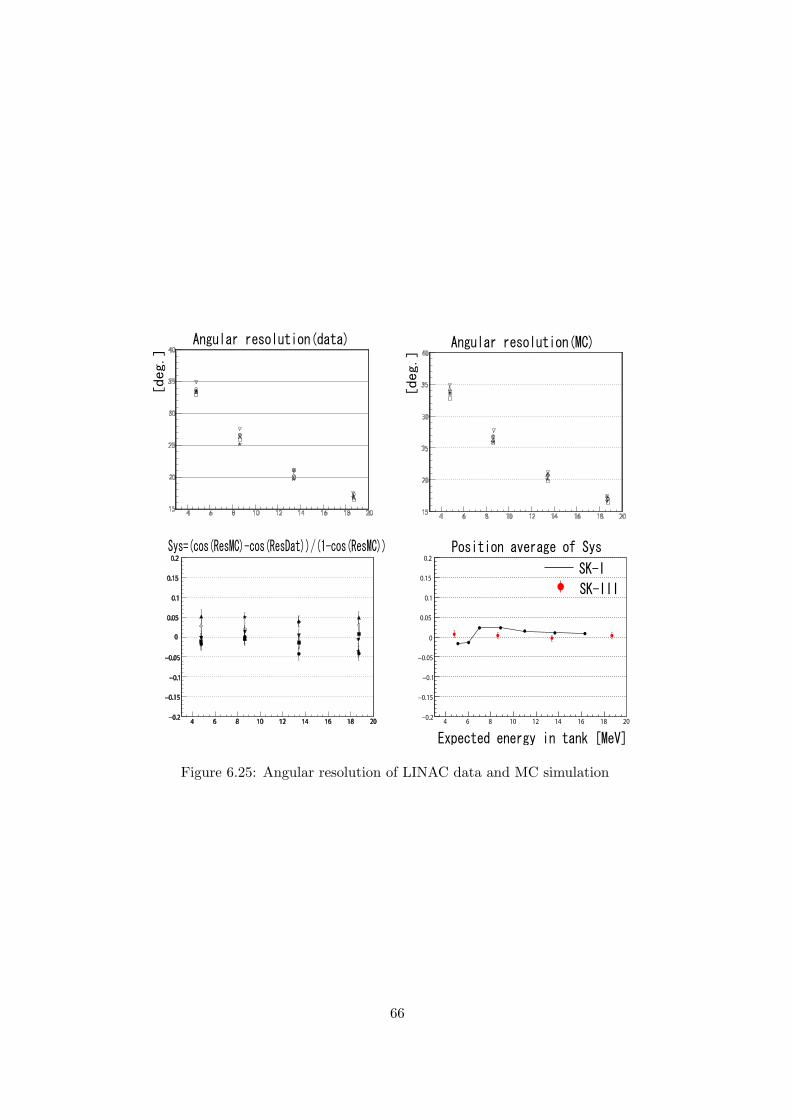
4 6 8 10 12 14 16 18 20−0.2
−0.15
−0.1
−0.05
0
0.05
0.1
0.15
0.2
4 6 8 10 12 14 16 18 20−0.2
−0.15
−0.1
−0.05
0
0.05
0.1
0.15
0.2
Figure 6.25: Angular resolution of LINAC data and MC simulation
66

Chapter 7
Data Analysis
The data for SK-III solar neutrino analysis were taken from August 5, 2006 to August 17,2008. SK-III has three periods with different hardware threshold settings. The explanation ofeach period is summarized in Table 7.1
7.1 Monitoring of Radon level
A major background for the lower energy region (total energy is less than 6.5 MeV) isradioactive impurities such as radon which are mixed in the pure water. To achieve the lowenergy threshold at 4.5 MeV, it is needed to reject such high radon concentration periods thathappened after water system maintenance or detector calibration, etc.. In order to do this,the radioactivity at different positions of the detector has been monitored by checking lowenergy event rate. Figure 7.1 shows how the low-energy event rate changes at the differentdetector positions. The high event rate periods coincide with the water system maintenance anddetector calibration. These high rate are caused by remaining radon in water. After removingthe high radioactivity periods, the sample for low-energy threshold analysis is obtained. Thecorresponding livetime is 298.2 days. Since the radon event only affect the low energy regionthe periods are not removed for sample with 6.5 MeV threshold whose livetime is 547.9 days.
7.2 Run definition
A basic unit of dataset is a run. Each run is at most 24 hours long, and divided into subrunswhich have usually 1 to 5 minutes long depending on the trigger rate.
Date (From Y/M/D to Y/M/D) Hardware thr. (mV) 100% eff. above: (MeV) livetime (days)
2006/08/05 - 2007/01/24 -302 6.5 121.7
2007/01/24 - 2008/04/17 -212 5.0 331.5
2008/04/17 - 2008/08/18 -186 4.5 94.8
Table 7.1: Summary of run periods with different hardware threshold values .
67
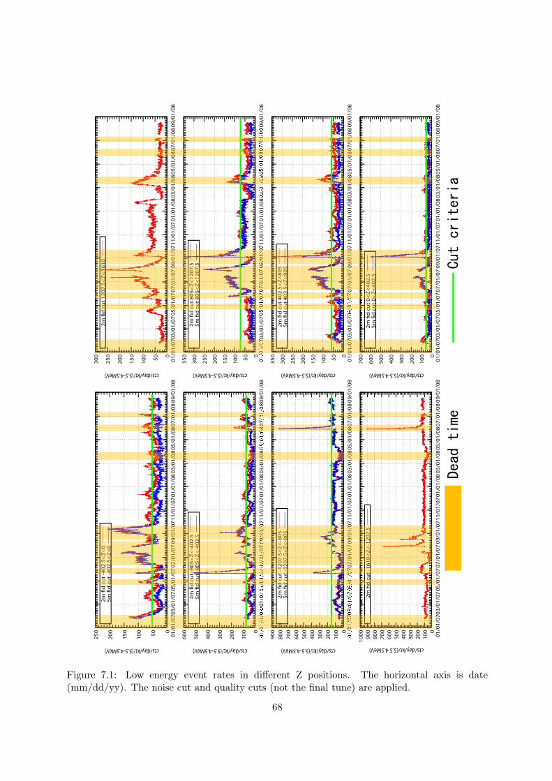
0
50
10
0
15
0
20
0
25
0
30
0
01
/01
/07
03
/01
/07
05
/01
/07
07
/01
/07
09
/01
/07
11
/01
/07
01
/01
/08
03
/01
/08
05
/01
/08
07
/01
/08
09
/01
/08
cts/day/kt/(5.5-4.5MeV)
2m
!d
cu
t 1
20
7.5
<Z
<1
61
0
0
50
10
0
15
0
20
0
25
0
30
0
35
0
03
/01
/07
11
/01
/07
01
/01
/08
09
/01
/08
cts/day/kt/(5.5-4.5MeV)
2m
!d
cu
t 8
05
<Z
<1
20
7.5
5m
!d
cu
t 8
05
<Z
<1
20
7.5
0
50
10
0
15
0
20
0
25
0
30
0
35
0
01
/01
/07
03
/01
/07
07
/01
/07
09
/01
/07
11
/01
/07
01
/01
/08
03
/01
/08
05
/01
/08
07
/01
/08
09
/01
/08
cts/day/kt/(5.5-4.5MeV)
2m
!d
cu
t 4
02
.5<
Z<
80
55
m !
d c
ut
40
2.5
<Z
<8
05
0
10
0
20
0
30
0
40
0
50
0
60
0
70
0
01
/01
/07
03
/01
/07
05
/01
/07
07
/01
/07
09
/01
/07
11
/01
/07
01
/01
/08
03
/01
/08
05
/01
/08
07
/01
/08
09
/01
/08
cts/day/kt/(5.5-4.5MeV)
2m
!d
cu
t 0
<Z
<4
02
.55
m !
d c
ut
0<
Z<
40
2.5
0
50
10
0
15
0
20
0
25
0
01
/01
/07
03
/01
/07
05
/01
/07
07
/01
/07
09
/01
/07
11
/01
/07
01
/01
/08
03
/01
/08
05
/01
/08
07
/01
/08
09
/01
/08
cts/day/kt/(5.5-4.5MeV)
2m
!d
cu
t -4
02
.5<
Z<
05
m !
d c
ut
-40
2.5
<Z
<0
0
10
0
20
0
30
0
40
0
50
0
60
0
11
/01
/07
01
/01
/08
03
/01
/08
09
/01
/08
cts/day/kt/(5.5-4.5MeV)
2m
!d
cu
t -8
05
<Z
<-4
02
.55
m !
d c
ut
-80
5<
Z<
-40
2.5
0
10
0
20
0
30
0
40
0
50
0
60
0
70
0
80
0
90
0
07
/01
/07
09
/01
/07
11
/01
/07
01
/01
/08
03
/01
/08
05
/01
/08
07
/01
/08
09
/01
/08
cts/day/kt/(5.5-4.5MeV)
2m
!d
cu
t -1
20
7.5
<Z
<-8
05
5m
!d
cu
t -1
20
7.5
<Z
<-8
05
0
10
0
20
0
30
0
40
0
50
0
60
0
70
0
80
0
90
0
10
00
01
/01
/07
03
/01
/07
05
/01
/07
07
/01
/07
09
/01
/07
11
/01
/07
01
/01
/08
03
/01
/08
05
/01
/08
07
/01
/08
09
/01
/08
cts/day/kt/(5.5-4.5MeV)
2m
!d
cu
t -1
61
0<
Z<
-12
07
.5
01
/01
/07
01
/01
/0
1/0
7
2m
!d
cu
t -1
61
0
2m
!d
cu
t -1
20
75
m !
d c
ut
-12
07
2m
!d
cu
t -8
05
<5
m !
d c
ut
-80
5<
01
/07
t -4
02
.5<
t -4
02
.5<
2m
!d
cu
t -1
61
0t
-16
10
t -1
20
7t
-12
07
2m
!d
cu
t -1
20
75
m !
d c
ut
-12
07
t -8
05
<t
-80
5<
07
5m
!d
cu
t -8
05
<5
m !
d c
ut
-80
5<
5m
!d
cu
t -8
05
<2
m !
d c
ut
-80
5<
5m
!d
cu
t -8
05
<5
m !
d c
ut
-80
5<
01
/07
t -4
02
.5<
t -4
02
.5<
2m
!d
cu
2m
!d
cu
5m
!d
cu
2m
!d
cu
5m
!d
cu
05
/01
/
2m
!d
cu
5m
!d
cu
2m
!d
cu
2m
!d
cu
2m
!d
cu
5m
!d
cu
2m
!d
cu
5m
!d
cu
2m
!d
cu
5m
!d
cu
05
/01
/
2m
!d
cu
5m
!d
cu
05
/01
/
2m
!d
cu
t -4
02
.5<
5m
!d
cu
t -4
02
.5<
t -1
61
0<
Z<
-12
07
/01
/07
09
/
t -1
20
7.5
<Z
<-8
0t
-12
07
.5<
Z<
-80
t -8
05
<Z
<-4
02
t -8
05
<Z
<-4
02
07
/01
/07
09
/
t -4
02
.5<
Z<
0t
-40
2.5
<Z
<0
<Z
<-1
2t
-16
10
09
/0
7/
.5<
Z<
-80
.5<
Z<
-80
t -1
20
7t
-12
07
Z<
-40
2Z
<-4
0209
/
t -8
05
<t
-80
5<
07
/
t -4
02
.5<
t -4
02
.5<
<Z
<-1
20
7.5
09
/01
/07
.5<
Z<
-80
5.5
<Z
<-8
05
Z<
-40
2.5
Z<
-40
2.5
09
/01
/07
<Z
<-1
20
7.
01
/07
09
/
.5<
Z<
-80
.5<
Z<
-800
1/0
7
Z<
-40
2.
Z<
-40
2.
09
/
01
/08
07
/
01
/08
07
/
07
/0
1/0
8
07
/0
1/0
8
07
/01
/
07
/01
/
07
/01
/0
7/0
1/
07
/01
/0
7/0
1/
01
/08
01
/08
01
/08
01
/08
01
/
01
/08
01
/
01
/08
01
/0
1/0
1/0
7
01
/01
/07
01
/01
/07
01
/01
/0
1/0
7
t 0
<Z
<4
02
t 0
<Z
<4
02
t 4
02
.5<
Z<
8t
40
2.5
<Z
<8
01
/07
t 1
20
7.5
<
t 8
05
<Z
<1
t 8
05
<Z
<1
t 0
<Z
<4
02
t 0
<Z
<4
02
t 0
<Z
<4
02
t 0
<Z
<4
02
t 4
02
.5<
Z<
8t
40
2.5
<Z
<8
t 4
02
.5<
Z<
8t
40
2.5
<Z
<8
01
/07
t 1
20
7.5
<
t 8
05
<Z
<1
t 8
05
<Z
<1
2m
!d
cu
t 0
<Z
<4
02
5m
!d
cu
t 0
<Z
<4
02
2m
!d
cu
5m
!d
cu
05
/01
/
2m
!d
cu
2m
!d
cu
5m
!d
cu
2m
!d
cu
t 0
<Z
<4
02
5m
!d
cu
t 0
<Z
<4
02
2m
!d
cu
5m
!d
cu
2m
!d
cu
t 4
02
.5<
Z<
85
m !
d c
ut
40
2.5
<Z
<8
2m
!d
cu
5m
!d
cu
05
/01
/
2m
!d
cu
2m
!d
cu
t 8
05
<Z
<1
5m
!d
cu
t 8
05
<Z
<1
07
/01
/07
09
/
t 0
<Z
<4
02
.5t
0<
Z<
40
2.5
t 4
02
.5<
Z<
80
5t
40
2.5
<Z
<8
05
07
/01
/07
09
/
t 1
20
7.5
<Z
<1
61
0
t 8
05
<Z
<1
20
7.
t 8
05
<Z
<1
20
7. 09
/0
7/
t 0
<Z
<4
02
t 0
<Z
<4
02
05
05
t 4
02
.5<
Z<
8t
40
2.5
<Z
<8
07
/0
9/
t 1
20
7.5
<Z
<1
61
0
t 8
05
<Z
<1
20
7.
t 8
05
<Z
<1
20
7. 09
/01
/07
09
/01
/07
Z<
16
10 0
1/0
70
9/
09
/01
/07
Z<
16
10
5 5
01
/08
07
/
01
/08
07
/
07
/0
1/0
8
01
/08
07
/
07
/01
/
07
/01
/
07
/01
/0
7/0
1/
07
/01
/
01
/08
01
/08
01
/08
01
/
01
/08
Figure 7.1: Low energy event rates in different Z positions. The horizontal axis is date(mm/dd/yy). The noise cut and quality cuts (not the final tune) are applied.
68
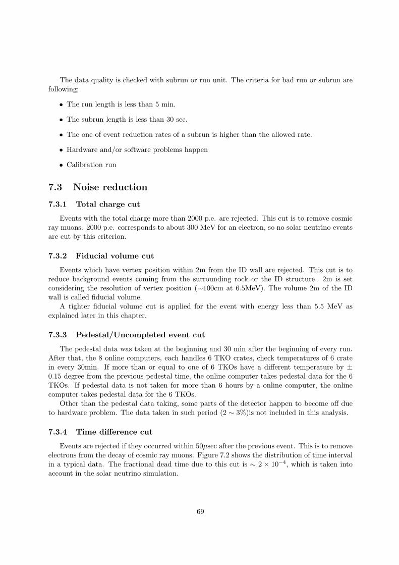
The data quality is checked with subrun or run unit. The criteria for bad run or subrun arefollowing;
• The run length is less than 5 min.
• The subrun length is less than 30 sec.
• The one of event reduction rates of a subrun is higher than the allowed rate.
• Hardware and/or software problems happen
• Calibration run
7.3 Noise reduction
7.3.1 Total charge cut
Events with the total charge more than 2000 p.e. are rejected. This cut is to remove cosmicray muons. 2000 p.e. corresponds to about 300 MeV for an electron, so no solar neutrino eventsare cut by this criterion.
7.3.2 Fiducial volume cut
Events which have vertex position within 2m from the ID wall are rejected. This cut is toreduce background events coming from the surrounding rock or the ID structure. 2m is setconsidering the resolution of vertex position (∼100cm at 6.5MeV). The volume 2m of the IDwall is called fiducial volume.
A tighter fiducial volume cut is applied for the event with energy less than 5.5 MeV asexplained later in this chapter.
7.3.3 Pedestal/Uncompleted event cut
The pedestal data was taken at the beginning and 30 min after the beginning of every run.After that, the 8 online computers, each handles 6 TKO crates, check temperatures of 6 cratein every 30min. If more than or equal to one of 6 TKOs have a different temperature by ±0.15 degree from the previous pedestal time, the online computer takes pedestal data for the 6TKOs. If pedestal data is not taken for more than 6 hours by a online computer, the onlinecomputer takes pedestal data for the 6 TKOs.
Other than the pedestal data taking, some parts of the detector happen to become off dueto hardware problem. The data taken in such period (2 ∼ 3%)is not included in this analysis.
7.3.4 Time difference cut
Events are rejected if they occurred within 50µsec after the previous event. This is to removeelectrons from the decay of cosmic ray muons. Figure 7.2 shows the distribution of time intervalin a typical data. The fractional dead time due to this cut is ∼ 2 × 10⁻⁴, which is taken intoaccount in the solar neutrino simulation.
69

1
10
102
103
104
105
2 3 4 5 6 7 8 9 10
Figure 7.2: Time difference to previous low energy triggered event. The first peak around 1µsecis due to ringing events after a high energy cosmic muon, and the second peak around 15µsecis due to after pulse events, and the third peak around 30µsec is so called ”after trigger” event,which is issued after HE triggered event.
7.3.5 OD event cut
Events with an OD trigger are rejected. An OD trigger is issued if the OD hits are morethan 19 his within a 200 nsec time window (see Figure 7.3). This is to remove cosmic ray muonevent with total p.e. less than 2000 p.e.
7.3.6 Noise cut
Event with high fraction of noise hits are rejected. This is to remove events due to electronicnoise. The fraction of noise hits is defined as follows;
NSratio = Nnoise/Ntotal (7.1)
where Nnoise is the number of hit PMTs with charge less than 0.5 p.e., and Ntotal is the totalnumber of hit PMTs. If NSratio is greater than 0.4, the event is rejected. Figure 7.4 showsNSratio distribution of a typical good run.
7.3.7 Goodness of vertex reconstruction cut
Events with poor vertex reconstruction are rejected. Figure 7.5 shows the goodness of thesecond vertex fitting [20]. If a event has goodness < 0.3, the event is rejected. Some brokenPMT made flash light. These flasher events are usually clustered in goodness < 0.3 region.
70
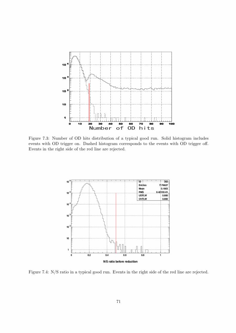
Figure 7.3: Number of OD hits distribution of a typical good run. Solid histogram includesevents with OD trigger on. Dashed histogram corresponds to the events with OD trigger off.Events in the right side of the red line are rejected.
Figure 7.4: N/S ratio in a typical good run. Events in the right side of the red line are rejected.
71
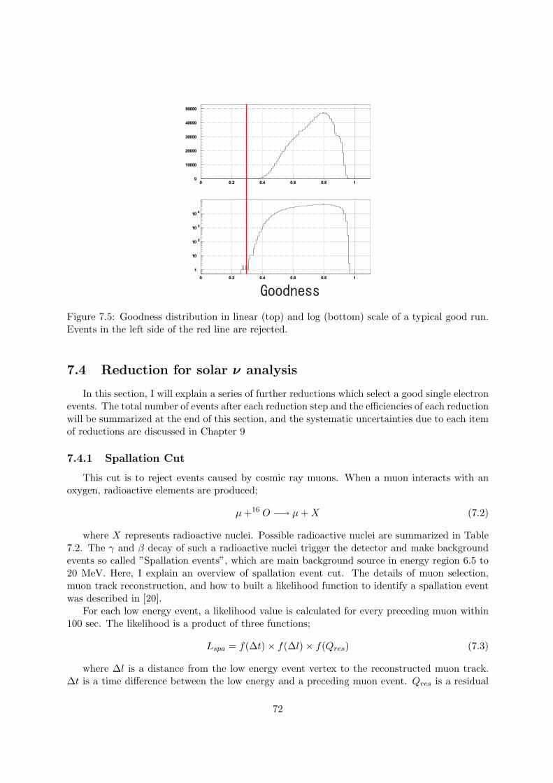
Figure 7.5: Goodness distribution in linear (top) and log (bottom) scale of a typical good run.Events in the left side of the red line are rejected.
7.4 Reduction for solar ν analysis
In this section, I will explain a series of further reductions which select a good single electronevents. The total number of events after each reduction step and the efficiencies of each reductionwill be summarized at the end of this section, and the systematic uncertainties due to each itemof reductions are discussed in Chapter 9
7.4.1 Spallation Cut
This cut is to reject events caused by cosmic ray muons. When a muon interacts with anoxygen, radioactive elements are produced;
µ +16 O −→ µ + X (7.2)
where X represents radioactive nuclei. Possible radioactive nuclei are summarized in Table7.2. The γ and β decay of such a radioactive nuclei trigger the detector and make backgroundevents so called ”Spallation events”, which are main background source in energy region 6.5 to20 MeV. Here, I explain an overview of spallation event cut. The details of muon selection,muon track reconstruction, and how to built a likelihood function to identify a spallation eventwas described in [20].
For each low energy event, a likelihood value is calculated for every preceding muon within100 sec. The likelihood is a product of three functions;
Lspa = f(∆t) × f(∆l) × f(Qres) (7.3)
where ∆l is a distance from the low energy event vertex to the reconstructed muon track.∆t is a time difference between the low energy and a preceding muon event. Qres is a residual
72

Isotope τ 12(sec) decay mode Kinetic Energy (MeV)
82He 0.119 β− 9.67 + 0.98(γ)
β− n 16%83Li 0.838 β− ∼ 1383B 0.77 β+ 13.993Li 0.178 β− 13.6 (50.5 % )
β− n (∼ 50 % )96C 0.127 β+ n 3∼15
113 Li 0.0085 β− 16∼20 (∼ 50 % )
β− n ∼ 16 (∼ 50 % )114 Be 13.8 β− 11.51 ( 54.7 % )
9.41 + 2.1 (γ) ( 31.4 % )114 Be 0.0236 β− 11.71125 B 0.0202 β− 13.37127 N 0.0110 β+ 16.32135 B 0.0174 β− 13.44138 O 0.0086 β+ 13.2 16.7145 B 0.0138 β− 14.55+6.09 (γ)156 C 2.449 β− 9.77 ( 36.8 % )
4.47+5.30 (γ)166 C 0.747 β− n ∼ 4167 N 7.13 β− 10.42 ( 28.0% )
4.29+6.13 (γ) (66.2% )
Table 7.2: Possible Spallation products in water [20]
73
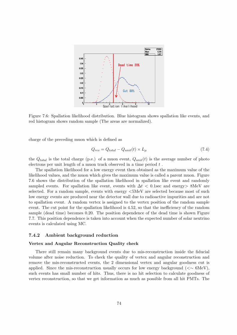
Figure 7.6: Spallation likelihood distribution. Blue histogram shows spallation like events, andred histogram shows random sample (The areas are normalized).
charge of the preceding muon which is defined as
Qres = Qtotal − Qunit(t) × Lµ (7.4)
the Qtotal is the total charge (p.e.) of a muon event, Qunit(t) is the average number of photoelectrons per unit length of a muon track observed in a time period t .
The spallation likelihood for a low energy event then obtained as the maximum value of thelikelihood values, and the muon which gives the maximum value is called a parent muon. Figure7.6 shows the distribution of the spallation likelihood in spallation like event and randomlysampled events. For spallation like event, events with ∆t < 0.1sec and energy> 8MeV areselected. For a random sample, events with energy <5MeV are selected because most of suchlow energy events are produced near the detector wall due to radioactive impurities and are notto spallation event. A random vertex is assigned to the vertex position of the random sampleevent. The cut point for the spallation likelihood is 4.52, so that the inefficiency of the randomsample (dead time) becomes 0.20. The position dependence of the dead time is shown Figure7.7. This position dependence is taken into account when the expected number of solar neutrinoevents is calculated using MC.
7.4.2 Ambient background reduction
Vertex and Angular Reconstruction Quality check
There still remain many background events due to mis-reconstruction inside the fiducialvolume after noise reduction. To check the quality of vertex and angular reconstruction andremove the mis-reconstructed events, the 2 dimensional vertex and angular goodness cut isapplied. Since the mis-reconstruction usually occurs for low energy background (<∼ 6MeV),such events has small number of hits. Thus, there is no hit selection to calculate goodness ofvertex reconstruction, so that we get information as much as possible from all hit PMTs. The
74

Figure 7.7: Spallation cut dead time depending on the detector position.
goodness vertex reconstruction is calculated using all hit PMT timing as follows,
GV =∑
e− 1
2
�(
τi(v⃗)−t0ω
)+(τi(v⃗)−t0
σ)� 2
∑e−
12(
τi(v⃗)−t0
ω)2
(7.5)
where τi(v⃗) = ti − |v⃗ − h⃗i|/c is a TOF subtracted hit time, and t0 is the fitted peak time ofτ distribution. The sums are over all hits.
The goodness of angular reconstruction can be tested by checking how the hit PMTs dis-tribute in space. In the case of a real electron event, the hit PMTs should reside uniformlyalong with Cherenkov ring toward the reconstructed direction. To check the uniformity, theKolomogorov-Smirnov test is applied. Figure 7.8 shows examples of event displays for a singleelectron event and a background event. Figure 7.8 also shows the distribution of azimuth angleof hit PMTs with respect to the reconstructed direction. The definition of goodness is the fullwidth of azimuth angle deviation which is given by
GA =max {∠uniform(i) − ∠Data(i)} − min {∠uniform(i) − ∠Data(i)}
2π(7.6)
where ∠uniform(i) is the azimuth angle of i-th hit PMT among the N50 assuming that the hitPMTs are uniformly distributed along with a Cherenkov cone (the dashed line in Figure7.8),and ∠Data(i) is that of real event (the closed circles in Figure7.8). As shown in the figures, agood event has a small value and a bad event has a large value.
The correlation between the vertex goodness GV and the angular goodness GA is shown infigure 7.9. Figure 7.9-(a) is a plot of real data which is just after the 1st reduction and stillcontains a lot of badly reconstructed events, and figure 7.9-(b) is that of solar neutrino MC. Asshown in the figure, we can separate a good single electron like event from background eventsby checking a quality factor which is a combination of the vertex goodness and the angulargoodness ovaQ (One dimensional variable of Vertex and Angular reconstruction Quality);
75
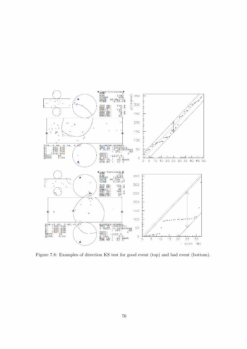
Figure 7.8: Examples of direction KS test for good event (top) and bad event (bottom).
76

Figure 7.9: Correlation of G2V (horizontal) and G2
A(vertical). Line indicate G2A = G2
V − 0.25
ovaQ ≡ G2V − G2
A (7.7)
Distributions of the quality factor for several energy are shown in figure 7.10. The cut criteriais following;
ovaQ > 0.29, 4.5 ≤ Energy < 5.0MeV
ovaQ > 0.25, 5.0 ≤ Energy < 7.5MeV
ovaQ > 0.20, Energy ≥ 7.5MeV
(7.8)
Flasher cut
If there is a PMT which emits light because of arch discharge on dynodes, such a PMTcauses background events so called ”flasher events”. The flasher event is characterized with alarge charge hit and many hits in the surrounding PMTs.
Figure 7.11 shows the maximum charge of a PMT in an event for the horizontal axis, andthe number of hits in the surrounding 24 PMTs. The cut criteria are also shown in the Figure7.11.
Hit Pattern cut
This cut is to select a clean single electron event. If additional γ-rays in an event, the hitpattern does not show a clear Cherenkov ring, then the reconstructed direction might not becorrect. To select a single electron event, a likelihood function is made from cos θdir,i distributionof the uniform electron MC event; Figure 7.14 shows examples of the Cherenkov ring probability
77

ovaq
0
0.1
0 0.2 0.4 0.6 0.8 1
4.5-5MeV
Data
B8MC
ovaq
0
0.1
0 0.2 0.4 0.6 0.8 1
5-5.5MeV
Data
B8MC
ovaq
0
0.1
0 0.2 0.4 0.6 0.8 1
5.5-6MeV
Data
B8MC
ovaq
0
0.1
0 0.2 0.4 0.6 0.8 1
6-6.5MeV
Data
B8MC
ovaq
0
0.1
0 0.2 0.4 0.6 0.8 1
6.5-7MeV
Data
B8MC
ovaq
0
0.1
0 0.2 0.4 0.6 0.8 1
7-7.5MeV
Data
B8MC
ovaq
0
0.1
0 0.2 0.4 0.6 0.8 1
7.5-8.5MeV
Data
B8MC
ovaq
0
0.1
0 0.2 0.4 0.6 0.8 1
8.5-9.5MeV
Data
B8MC
Figure 7.10: ovaQ distribution of different energy region.
78
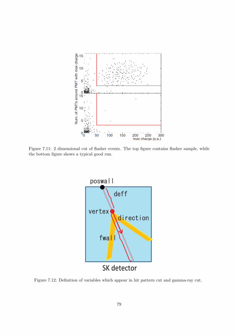
Figure 7.11: 2 dimensional cut of flasher events. The top figure contains flasher sample, whilethe bottom figure shows a typical good run.
SK detector
Figure 7.12: Definition of variables which appear in hit pattern cut and gamma-ray cut.
79

functions for several energy regions. The definition of Cherenkov ring probability is
P (Energy, vertex, diretion) =1
N50
N50∑i
log(f(Energy, cos θdir,i, fwall)) (7.9)
where fwall is the distance from the event vertex to the detector wall (See Figure 7.12) along withthe reconstructed direction, and probability functions f(Energy, cos θdir.i, fwall) are obtainedfrom single electron MC with different energies. To determine the cut point of P , the significanceis calculated as
Significance(P ) =
∫ PP0
MC(P ′)dP ′√∫ PP0
BG(P ′)dP ′(7.10)
where MC(P ) and BG(P ) are distributions of the Cherenkov ring probability obtained fromsingle electron MC and control sample of real data and P0 is the likelihood value at the left edgeof Figure 7.13. The obtained cut criteria which give maximum significance for different energyregions are
P > −1.88, 6.5MeV ≤ Energy < 8.0MeV
P > −1.86, 8.0MeV ≤ Energy < 12.0MeV
P > −1.95, 12.0MeV ≤ Energy
(7.11)
Since, for an event whose energy is less than 6.5 MeV, the distributions of likelihood for dataand solar neutrino MC become the same (see Figure 7.14), I decided not to use this cut for theenergy region.
Fiducial volume cut using the second vertex fitter
The result of second vertex reconstruction is checked here. If the reconstruction returns avertex position outside of the fiducial volume (2m inside of the ID wall), the event is rejected.
7.4.3 Gamma-ray cut
This cut is to reject events induced by gamma-ray which are from the PMTs or the detectorwall. To eliminate the background, events with direction inward from the wall are rejected. Thecriteria for event energy ≥ 6.5MeV are{
deff > 650cm, 6.5MeV ≤ Energy < 8.0MeV
deff > 400cm, 8.0MeV ≤ Energy(7.12)
where deff is the distance from the wall in the direction of the reconstructed event (see Figure7.12), and this cut points are obtained by calculation of significance as in Equation 7.10 but thesignificance here is a function of deff .
Figure 7.15 shows the distribution of deff for different energy regions. Because the radioac-tive background (energy <6.5 MeV ) is not uniformly distributed in the detector (see ??), atighter fiducial volume cut is needed. Considering the tighter fiducial volume which will betuned in the later step, events in the central area (z > −5m,r< 13m) are selected to tune thegamma-ray cut point of deff for energy < 6.5MeV region. Then, for this energy region, different
80
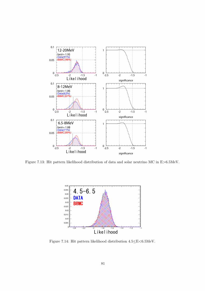
0
0.05
0.1
-2.5 -2 -1.5 -1
12-20MeVbest=-1.95Data(91%)B8MC(98%)
signi cance
0
1
-2.5 -2 -1.5 -1
0
0.05
0.1
-2.5 -2 -1.5 -1
8-12MeVbest=-1.86Data(62%)B8MC(87%)
signi cance
0
1
-2.5 -2 -1.5 -1
0
0.05
0.1
-2.5 -2 -1.5 -1
6.5-8MeVbest=-1.88Data(71%)B8MC(89%)
signi cance
0
1
-2.5 -2 -1.5 -1
Figure 7.13: Hit pattern likelihood distribution of data and solar neutrino MC in E>6.5MeV.
−2.4 −2.2 −2 −1.8 −1.6 −1.4 −1.2 −10
0.005
0.01
0.015
0.02
0.025
0.03
0.035
0.04
0.045
0.05
Figure 7.14: Hit pattern likelihood distribution 4.5≤E<6.5MeV.
81
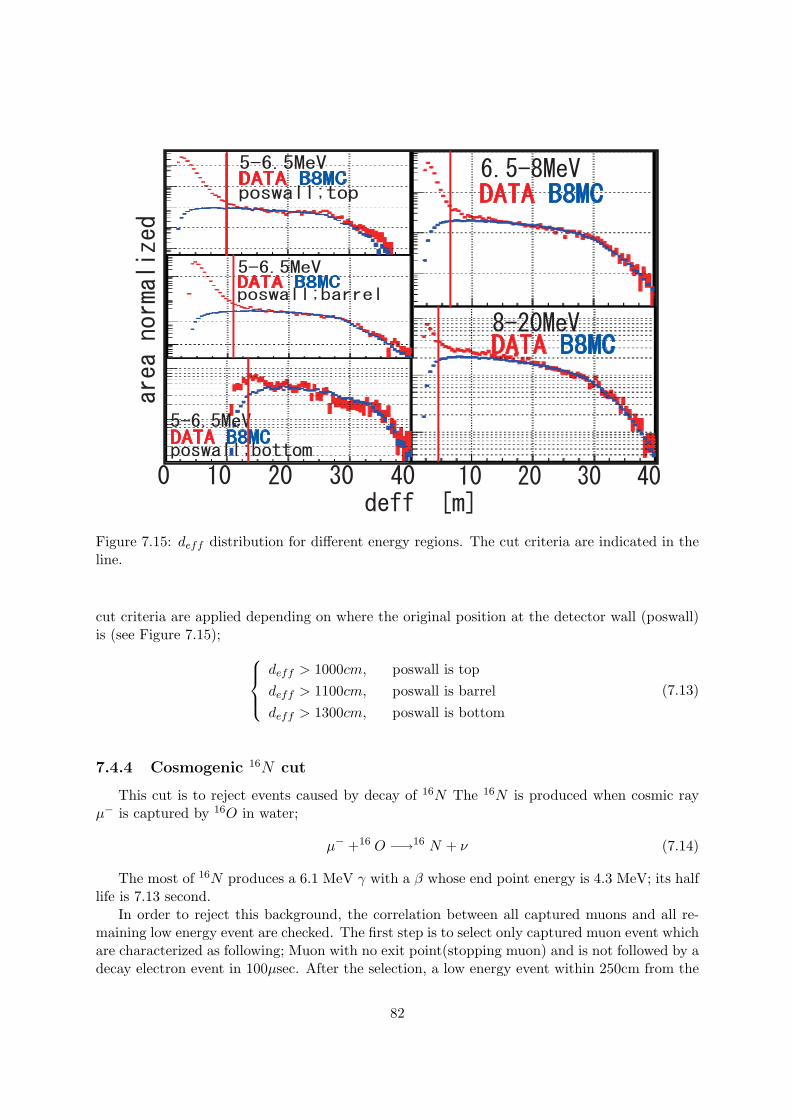
Figure 7.15: deff distribution for different energy regions. The cut criteria are indicated in theline.
cut criteria are applied depending on where the original position at the detector wall (poswall)is (see Figure 7.15);
deff > 1000cm, poswall is topdeff > 1100cm, poswall is barreldeff > 1300cm, poswall is bottom
(7.13)
7.4.4 Cosmogenic 16N cut
This cut is to reject events caused by decay of 16N The 16N is produced when cosmic rayµ− is captured by 16O in water;
µ− +16 O −→16 N + ν (7.14)
The most of 16N produces a 6.1 MeV γ with a β whose end point energy is 4.3 MeV; its halflife is 7.13 second.
In order to reject this background, the correlation between all captured muons and all re-maining low energy event are checked. The first step is to select only captured muon event whichare characterized as following; Muon with no exit point(stopping muon) and is not followed by adecay electron event in 100µsec. After the selection, a low energy event within 250cm from the
82
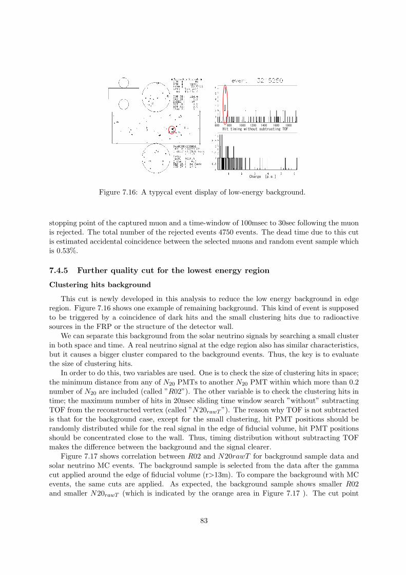
Figure 7.16: A typycal event display of low-energy background.
stopping point of the captured muon and a time-window of 100msec to 30sec following the muonis rejected. The total number of the rejected events 4750 events. The dead time due to this cutis estimated accidental coincidence between the selected muons and random event sample whichis 0.53%.
7.4.5 Further quality cut for the lowest energy region
Clustering hits background
This cut is newly developed in this analysis to reduce the low energy background in edgeregion. Figure 7.16 shows one example of remaining background. This kind of event is supposedto be triggered by a coincidence of dark hits and the small clustering hits due to radioactivesources in the FRP or the structure of the detector wall.
We can separate this background from the solar neutrino signals by searching a small clusterin both space and time. A real neutrino signal at the edge region also has similar characteristics,but it causes a bigger cluster compared to the background events. Thus, the key is to evaluatethe size of clustering hits.
In order to do this, two variables are used. One is to check the size of clustering hits in space;the minimum distance from any of N20 PMTs to another N20 PMT within which more than 0.2number of N20 are included (called ”R02”). The other variable is to check the clustering hits intime; the maximum number of hits in 20nsec sliding time window search ”without” subtractingTOF from the reconstructed vertex (called ”N20rawT ”). The reason why TOF is not subtractedis that for the background case, except for the small clustering, hit PMT positions should berandomly distributed while for the real signal in the edge of fiducial volume, hit PMT positionsshould be concentrated close to the wall. Thus, timing distribution without subtracting TOFmakes the difference between the background and the signal clearer.
Figure 7.17 shows correlation between R02 and N20rawT for background sample data andsolar neutrino MC events. The background sample is selected from the data after the gammacut applied around the edge of fiducial volume (r>13m). To compare the background with MCevents, the same cuts are applied. As expected, the background sample shows smaller R02and smaller N20rawT (which is indicated by the orange area in Figure 7.17 ). The cut point
83

Figure 7.17: Correlation between R02 and N20rawT for background sample (left) and solarneutrino MC events (right).
is obtained from one dimensional distribution of R02 × N20rawT /Neff . The significance as afunction of R02 × N20rawT /Neff becomes maximum at R02 × N20rawT /Neff = 75 (see Figure7.18). Following is a summary of cut criteria of this new cut;
R02 × N20rawT /Neff > 75 and r2 > 180m2 for 5.5 ≤E< 6.5 MeVR02 × N20rawT /Neff > 75 and r2 > 155m2 for 5.0 ≤E< 5.5 MeVR02 × N20rawT /Neff > 75 and r2 > 120m2 for 4.5 ≤E< 5.0 MeV
(7.15)
After these cut applied, the vertex distributions in low-energy events are shown in Figure7.19.
Tighter fiducial volume cut
This cut is to reject the remaining background in the edge region. As shown in Figure 7.19,background events in the bottom region still remain after the cluster cut. This nonuniformityof the vertex distribution of background makes the angular distribution of the backgrounddistorted, which causes a large systematic uncertainty for day-night asymmetry of solar neutrinoflux.
To set a tight fiducial volume, the significance as a function of detector radius is calculated.Based on the significance calculation, the final value of fiducial volume is obtained for eachenergy region which is shown in Figure 7.19:
4.5 − 5MeV : (r2 < 180m2andz > −3m)or(r2 < 120m2and − 7 < z < 3m) = 12.3kton
5 − 5.5MeV : (r2 < 180m2andz > −7.5m) = 13.3kton
5.5 − 20Mev : no tight fiducial volume cut = 22.5kton
84

Figure 7.18: Distribution of R02 × N20rawT /Neff and the significance.
Figure 7.19: Vertex distribution of low-energy events. The tight fiducial volume is shown by thered box: 12.3kton for 4.5-5MeV, 13.3kton for 5-5.5MeV and 22.5kton 5.5-20MeV.
85

Figure 7.20: Number of event after each reduction step as a function of energy. Precut in SK-I(open circle) means noise reduction. For and SK-III(blue) there still remained lots of low-energyevents due to FRP. Thus, ovaQ > 0.2 is applied for all events, and this is called precut in SK-III.
7.5 Summary of Reduction step
Figure 7.20 shows the energy spectrum after each step of the reductions and Figure 7.21 showsthe remaining efficiency of 8B solar neutrino MC with respect to the reconstructed energy. Whilethe event rate in the real data as a function of energy is the same as SK-I, the cut efficienciesare improved by 10% in the final data sample. For 4.5-5MeV region, while the efficiency getsworse by about 30% compared to SK-I, the background is reduced by about 80%, which enablesto observe the solar neutrino signals in that energy region with better signal to noise ratio. Thenumber of events after each reduction step is summarized in Table 7.3 (real data) and 7.4.
86

Figure 7.21: Reduction efficiency for the solar neutrino MC simulation. Color lines show SK-IIIand Makers show SK-I (From top; after SLE trigger, noise reduction, spallation cut, ambientBG reduction, and final data sample)
Reduction step 4.5-20.0 MeV 5.0-20.0 MeV 6.5-20.0 MeV
Precut 10162637 2381464 669641Spallation cut 8324066 1861770 114350ovaQ 1795878 866835 100470Second fidv. cut 1609465 734843 89808Hit pattern cut 58187Gamma ray cut 89096 54820 4314616N cut 89096 54351 39879Cluster cut 67774 42916Tight fidv. cut 13346 24311
Final 13346 24311 39879
Table 7.3: Reduction results of data
87
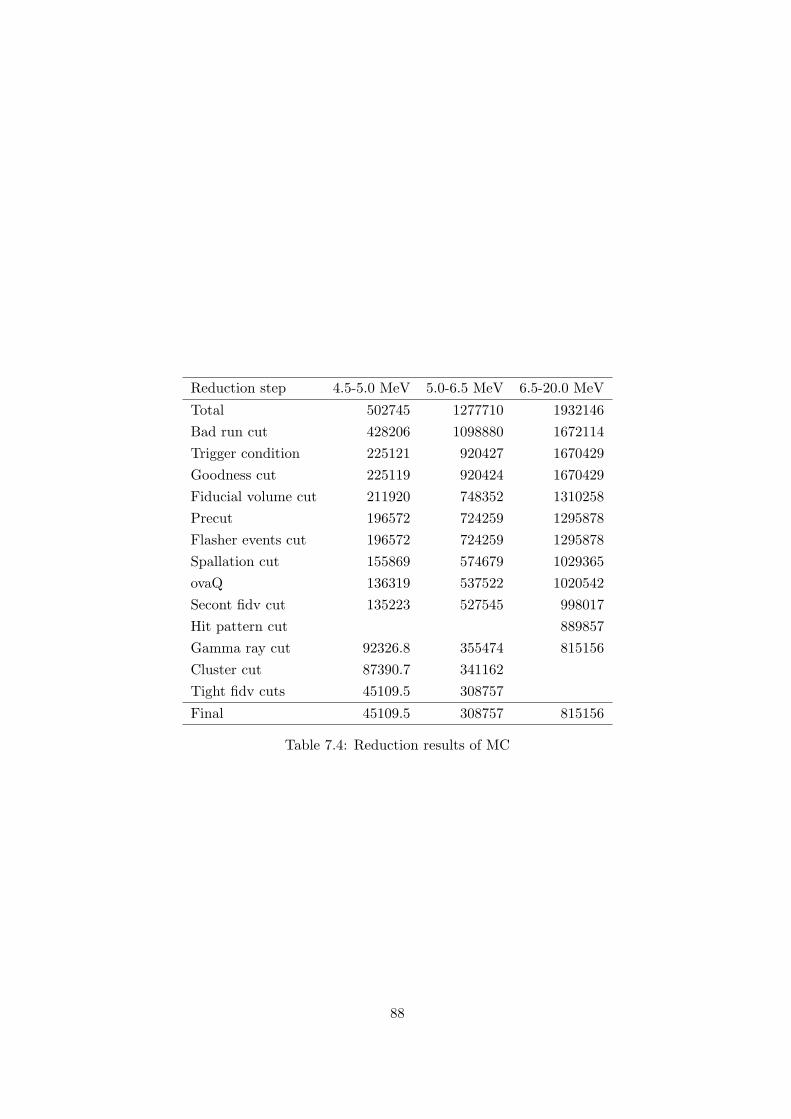
Reduction step 4.5-5.0 MeV 5.0-6.5 MeV 6.5-20.0 MeV
Total 502745 1277710 1932146Bad run cut 428206 1098880 1672114Trigger condition 225121 920427 1670429Goodness cut 225119 920424 1670429Fiducial volume cut 211920 748352 1310258Precut 196572 724259 1295878Flasher events cut 196572 724259 1295878Spallation cut 155869 574679 1029365ovaQ 136319 537522 1020542Secont fidv cut 135223 527545 998017Hit pattern cut 889857Gamma ray cut 92326.8 355474 815156Cluster cut 87390.7 341162Tight fidv cuts 45109.5 308757
Final 45109.5 308757 815156
Table 7.4: Reduction results of MC
88

Chapter 8
Signal extraction
8.1 Solar angle fitting
The strongest information which is used to extract solar neutrino signal from the final sampleis the direction of the recoil electrons because the direction of the recoil electron is stronglycorrelated with the direction of the incident neutrino. Thus, by checking the cosine of thedirection from the Sun and the event direction (cos θsun), the solar neutrino signals can beextracted. The signal extraction is done by an extended maximum likelihood fit [43] with dataand the solar neutrino MC events distributions. The likelihood function is
L = e−(∑
i Bi+S)Nbin∏i=1
ni∏j=1
(Bi · bij + S · Yi · sij) (8.1)
where Nbin = 22 is the number of bins between 4.5 MeV and 20.0 MeV: 19 energy bins of0.5 MeV between 4.5 and 14.0 MeV, two energy bins of 1 MeV between 14.0 and 16.0 MeV,and one bin between 16.0 and 20.0 MeV 1 . and ni is the number of observed events in thei-th energy bin. S and Bi are free parameters to be fitted and represent the total number ofsolar neutrino events and the number of background in the i-th energy bin. Yi is the expectedfraction of signal events in the i-th energy bin which will be explained in the next section. Theprobability density functions bij and sij describe the expected shapes of the background andrecoil electron signal respectively, and are defined for each energy bin as a function of the solarangle.
bij = u(cos θij) (8.2)
sij = p(cos θij , Eij) (8.3)
where θij and Eij are a solar angle and energy of j-th event in i-th energy bin. The definition ofthe solar angle (θj ≡ θSun) is shown in Figure 8.1. The background shape is not completely flatdue to the cylindrical shape of the detector. To estimate the shape of background, at first, thezenith angle and azimuthal distributions of real data (cos θsun < 0.7 is imposed to avoid solarsignal) are fitted with an eighth-order polynomial. Then, the expected solar angle distributioncan be obtained from the fitted zenith and azimuthal distributions by generating a toy MC. The
1If the threshold is 5.0 MeV, the number of bins are 21 bins: 18 energy bins of 0.5 MeV between 5 and 14.0MeV, two energy bins of 1 MeV between 14.0 and 16.0 MeV, and one bin between 16.0 and 20.0 MeV. That is,i = 2 ∼ 22 is for 5MeV threshold, and i = 5 ∼ 22 is for 6.5MeV threshold.
89
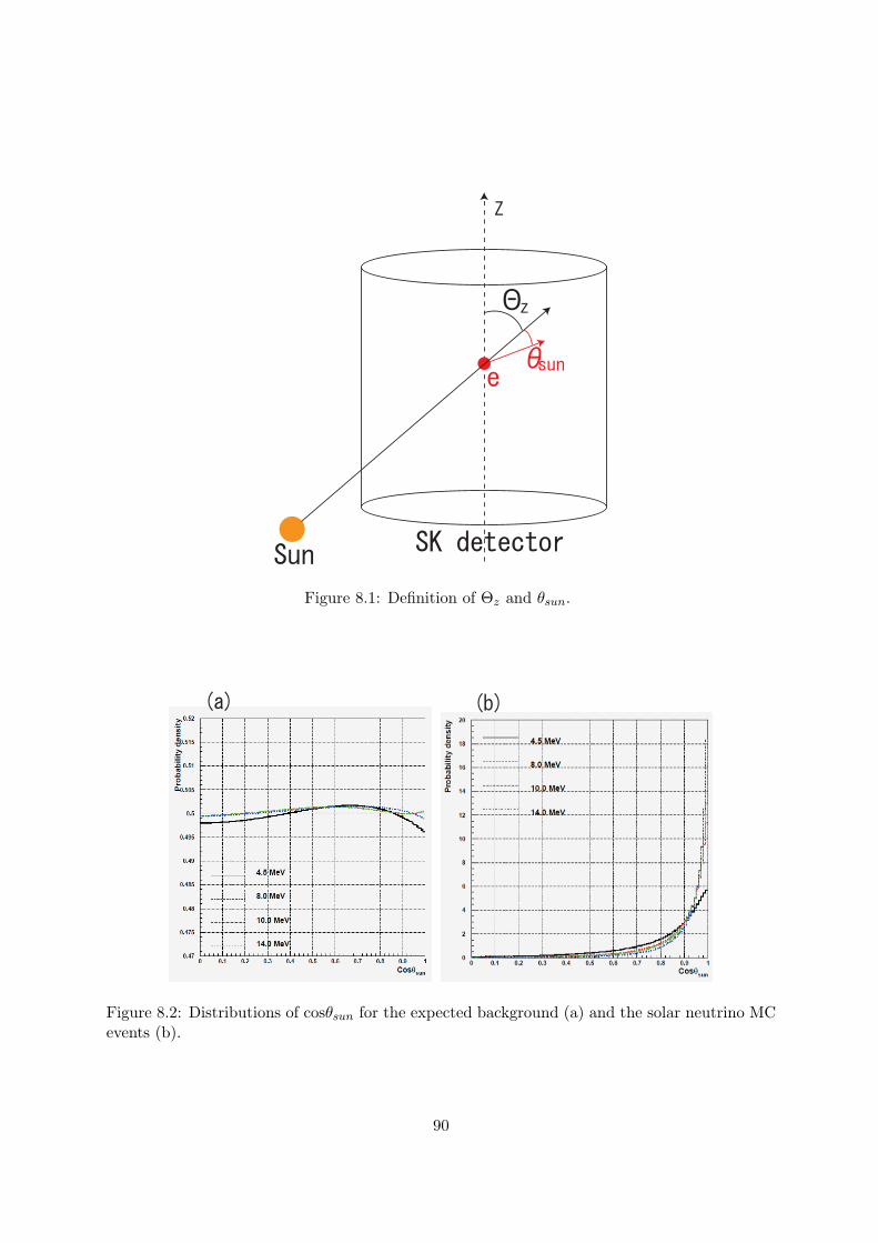
Figure 8.1: Definition of Θz and θsun.
Figure 8.2: Distributions of cosθsun for the expected background (a) and the solar neutrino MCevents (b).
90
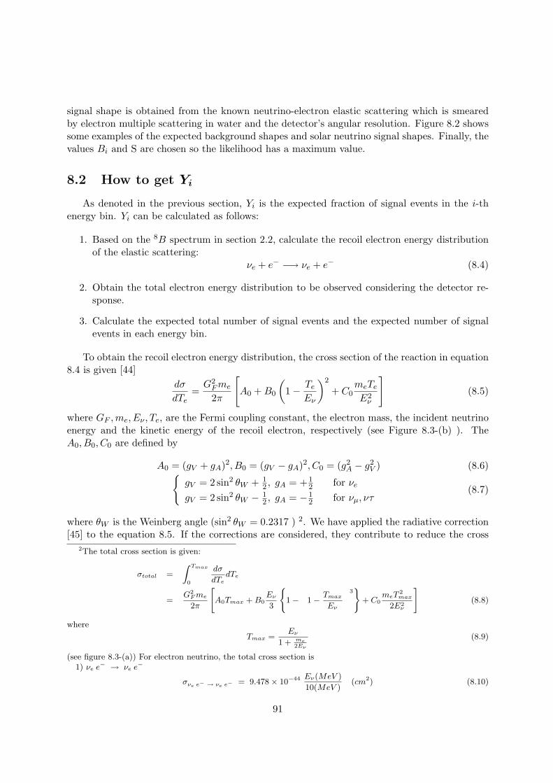
signal shape is obtained from the known neutrino-electron elastic scattering which is smearedby electron multiple scattering in water and the detector’s angular resolution. Figure 8.2 showssome examples of the expected background shapes and solar neutrino signal shapes. Finally, thevalues Bi and S are chosen so the likelihood has a maximum value.
8.2 How to get Yi
As denoted in the previous section, Yi is the expected fraction of signal events in the i-thenergy bin. Yi can be calculated as follows:
1. Based on the 8B spectrum in section 2.2, calculate the recoil electron energy distributionof the elastic scattering:
νe + e− −→ νe + e− (8.4)
2. Obtain the total electron energy distribution to be observed considering the detector re-sponse.
3. Calculate the expected total number of signal events and the expected number of signalevents in each energy bin.
To obtain the recoil electron energy distribution, the cross section of the reaction in equation8.4 is given [44]
dσ
dTe=
G2F me
2π
[A0 + B0
(1 − Te
Eν
)2
+ C0meTe
E2ν
](8.5)
where GF ,me, Eν , Te, are the Fermi coupling constant, the electron mass, the incident neutrinoenergy and the kinetic energy of the recoil electron, respectively (see Figure 8.3-(b) ). TheA0, B0, C0 are defined by
A0 = (gV + gA)2, B0 = (gV − gA)2, C0 = (g2A − g2
V ) (8.6){gV = 2 sin2 θW + 1
2 , gA = +12 for νe
gV = 2 sin2 θW − 12 , gA = −1
2 for νµ, ντ(8.7)
where θW is the Weinberg angle (sin2 θW = 0.2317 ) 2. We have applied the radiative correction[45] to the equation 8.5. If the corrections are considered, they contribute to reduce the cross
2The total cross section is given:
σtotal =
∫ Tmax
0
dσ
dTedTe
=G2
F me
2π
[A0Tmax + B0
Eν
3
{1 −�
1 − Tmax
Eν
� 3}
+ C0meT
2max
2E2ν
](8.8)
where
Tmax =Eν
1 + me2Eν
(8.9)
(see figure 8.3-(a)) For electron neutrino, the total cross section is1) νe e− → νe e−
σνe e− → νe e− = 9.478 × 10−44 Eν(MeV )
10(MeV )(cm2) (8.10)
91
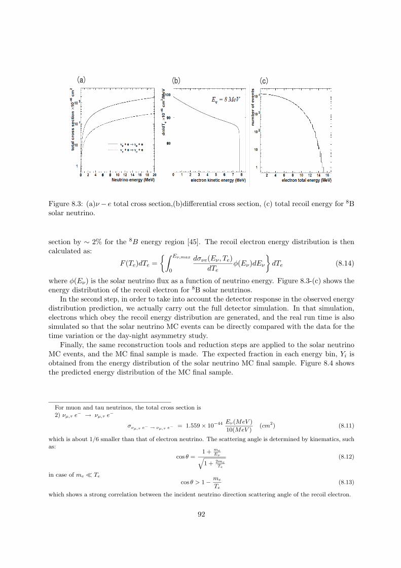
Figure 8.3: (a)ν − e total cross section,(b)differential cross section, (c) total recoil energy for 8Bsolar neutrino.
section by ∼ 2% for the 8B energy region [45]. The recoil electron energy distribution is thencalculated as:
F (Te)dTe ={∫ Eν,max
0
dσνe(Eν , Te)dTe
ϕ(Eν)dEν
}dTe (8.14)
where ϕ(Eν) is the solar neutrino flux as a function of neutrino energy. Figure 8.3-(c) shows theenergy distribution of the recoil electron for 8B solar neutrinos.
In the second step, in order to take into account the detector response in the observed energydistribution prediction, we actually carry out the full detector simulation. In that simulation,electrons which obey the recoil energy distribution are generated, and the real run time is alsosimulated so that the solar neutrino MC events can be directly compared with the data for thetime variation or the day-night asymmetry study.
Finally, the same reconstruction tools and reduction steps are applied to the solar neutrinoMC events, and the MC final sample is made. The expected fraction in each energy bin, Yi isobtained from the energy distribution of the solar neutrino MC final sample. Figure 8.4 showsthe predicted energy distribution of the MC final sample.
For muon and tau neutrinos, the total cross section is2) νµ,τ e− → νµ,τ e−
σνµ,τ e− → νµ,τ e− = 1.559 × 10−44 Eν(MeV )
10(MeV )(cm2) (8.11)
which is about 1/6 smaller than that of electron neutrino. The scattering angle is determined by kinematics, suchas:
cos θ =1 + me
Eν√1 + 2me
Te
(8.12)
in case of me ≪ Te
cos θ > 1 − me
Te(8.13)
which shows a strong correlation between the incident neutrino direction scattering angle of the recoil electron.
92

Figure 8.4: Energy spectrum of the solar neutrino MC final sample. The 8B flux from BP04 SSMand Winter spectrum is used for red histogram and Ortiz spectrum is used for black histogram.The reduction efficiency in Figure 7.21 is considered. They agree within 5%.
93
Chapter 9
Systematic Uncertainties
9.1 Energy scale
In order to study how the energy scale systematic uncertainty (0.53%) affect to the fluxvalue, the difference of the Yi is obtained first. By changing the energy of each solar ν MC eventby + or - 0.53% after the energy reconstruction, Y scale+
i and Y scale−i are calculated. Using the
Y scale+i and Y scale−
i , the solar angle fittings are carried out. Then it turns out that the 0.53%scale shift makes ±1.4% difference on the total flux in the 5.0-20.0 MeV electron total energyregion.
For the day-night asymmetry study, I only take into account the angular dependence ofenergy scale uncertainty (0.25%) because the other systematic uncertainties of energy scalewould be canceled out in the calculation of the asymmetry factor ((ΦD − ΦN )/0.5(ΦD + ΦN )).In the same way, Y DN+
i and Y DN−i are calculated with + or - 0.25% scale shift. As the result
of the solar angle fittings, the systematic uncertainty of the day-night asymmetry is estimatedas ±1.3% in the 5.0-20MeV region.
Since the water transparency varies in time, the energy scale uncertainty depending on thewater transparency (0.21%) should be contributed to the uncertainty to the seasonal study. Itis estimated as ±1.3%.
9.2 Energy resolution
In order to estimate the effect of the systematic uncertainty of the energy resolution (±2.5%)on the total flux, the prediction of observed energy spectrum is obtained not from the full detectorsimulation but from the calculation:
F(Eobs) ={∫ Emax
0F (Ee)R(Ee, Eobs)dEe
}dEobs (9.1)
where Eobs,F(Eobs) are observed energy and the calculated observed energy spectrum, Ee istotal energy of recoil electron, and F (Ee) is the recoil energy spectrum calculated in equation8.14. R(Ee, Eobs) is the detector response function:
R(Ee, Eobs) =1√
2πσ(Ee)2exp
(−(Ee − Eobs)2
σ(Ee)2
)(9.2)
94
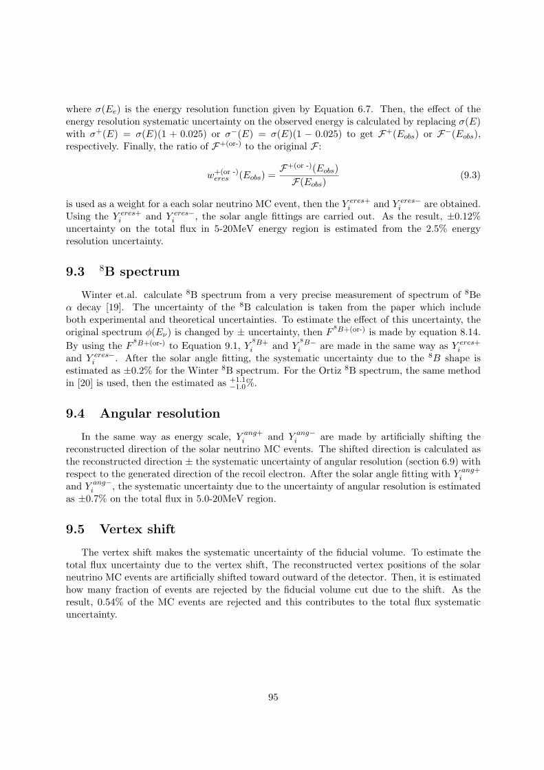
where σ(Ee) is the energy resolution function given by Equation 6.7. Then, the effect of theenergy resolution systematic uncertainty on the observed energy is calculated by replacing σ(E)with σ+(E) = σ(E)(1 + 0.025) or σ−(E) = σ(E)(1 − 0.025) to get F+(Eobs) or F−(Eobs),respectively. Finally, the ratio of F+(or-) to the original F :
w+(or -)eres (Eobs) =
F+(or -)(Eobs)F(Eobs)
(9.3)
is used as a weight for a each solar neutrino MC event, then the Y eres+i and Y eres−
i are obtained.Using the Y eres+
i and Y eres−i , the solar angle fittings are carried out. As the result, ±0.12%
uncertainty on the total flux in 5-20MeV energy region is estimated from the 2.5% energyresolution uncertainty.
9.3 8B spectrum
Winter et.al. calculate 8B spectrum from a very precise measurement of spectrum of 8Beα decay [19]. The uncertainty of the 8B calculation is taken from the paper which includeboth experimental and theoretical uncertainties. To estimate the effect of this uncertainty, theoriginal spectrum ϕ(Eν) is changed by ± uncertainty, then F
8B+(or-) is made by equation 8.14.By using the F
8B+(or-) to Equation 9.1, Y8B+i and Y
8B−i are made in the same way as Y eres+
i
and Y eres−i . After the solar angle fitting, the systematic uncertainty due to the 8B shape is
estimated as ±0.2% for the Winter 8B spectrum. For the Ortiz 8B spectrum, the same methodin [20] is used, then the estimated as +1.1
−1.0%.
9.4 Angular resolution
In the same way as energy scale, Y ang+i and Y ang−
i are made by artificially shifting thereconstructed direction of the solar neutrino MC events. The shifted direction is calculated asthe reconstructed direction ± the systematic uncertainty of angular resolution (section 6.9) withrespect to the generated direction of the recoil electron. After the solar angle fitting with Y ang+
i
and Y ang−i , the systematic uncertainty due to the uncertainty of angular resolution is estimated
as ±0.7% on the total flux in 5.0-20MeV region.
9.5 Vertex shift
The vertex shift makes the systematic uncertainty of the fiducial volume. To estimate thetotal flux uncertainty due to the vertex shift, The reconstructed vertex positions of the solarneutrino MC events are artificially shifted toward outward of the detector. Then, it is estimatedhow many fraction of events are rejected by the fiducial volume cut due to the shift. As theresult, 0.54% of the MC events are rejected and this contributes to the total flux systematicuncertainty.
95

Figure 9.1: The difference of the ovaQ cut efficiency (MC-DATA)/MC of LINAC.
9.6 Reduction
9.6.1 ovaQ cut
Figure 9.1 shows the difference of the efficiency of ovaQ cut using the LINAC data andMC. To estimate the systematic uncertainty of the total flux due to the ovaQ cut, this energydependence of the efficiency is taken into account. As the result, ±0.4% uncertainty to the totalflux in 5.0-20MeV energy region is found.
9.6.2 Hit pattern cut
Figure 9.2 shows the difference of the inefficiency of the hit pattern cut using the LINAC dataand MC. As seen in the figure, the efficiency difference between data and MC agree within 0.25%.This maximum discrepancy 0.25% is taken as the uncertainty to the total flux, conservatively.
9.6.3 Second vertex cut
The reconstructed vertex shift using the second fitter is also taken into account to estimatethe systematic uncertainty on the flux. The estimation is done in the same way as the BONSAIvertex fitter, resulting 0.45% of uncertainty should contribute to the total flux.
9.7 Spallation cut
The same uncertainties as SK-I [20] is taken in this thesis. This is because the origin of thesystematic uncertainty of spallation cut is mainly due to the characteristics of the muon suchas rate, energy, arrival direction, and thus, the uncertainly should not depend on each phases ofthe experiment. The estimated valuses are 0.2% on the total flux in 5.0-20MeV region and 0.1% for the time dependence part.
96

Figure 9.2: The difference of hit pattern cut efficiency (MC-DATA)/MC of LINAC.
9.8 Gamma ray cut
The vertex shift and the difference in the angular resolution measured by LINAC make somebias to the gamma cut efficiency. To estimate the effect, first, the reconstructed vertex anddirection of solar neutrino MC events are shifted with the difference of the vertex and angularresolution systematic uncertainties between data and MC as shown in Figure 9.3. Second,the gamma cut efficiencies of the shifted MC sample and the original MC sample are compared.Then, the systematic uncertainty due to the gamma cut is estimated as ±0.25% for the total flux,and ±0.2% for the day-night asymmetry. For the uncertainly of spectrum, ±0.1% uncertaintyis estimated.
9.9 Background shape
The systematic uncertainty due to the background shape prediction is estimated. As in thesection 8.1, the solar angle distribution is fitted with the non-flat background shape. To get thenon-flat background shape, not only the distribution of z-direction but also the distribution ofphi direction is fitted. To estimate the systematic uncertainty, the background shape assumingflat ϕ distribution is made and then the solar angle fitting is carried out with the backgroundshape. The difference of the fitting results between these two types of background shapes aretaken as the systematic uncertainty, which is 0.07% for the total flux and 0.4% for the day-nightasymmetry.
9.10 Signal extraction method
To check how the signal extraction method biases the flux value, the solar angle fit is appliedto dummy data which have known number of signal and background events. As the result,±0.7% difference is found between the input and the output number of signal events for thetotal flux, and ±2% difference is found especially in the 5.0 < E < 5.5MeV region.
97
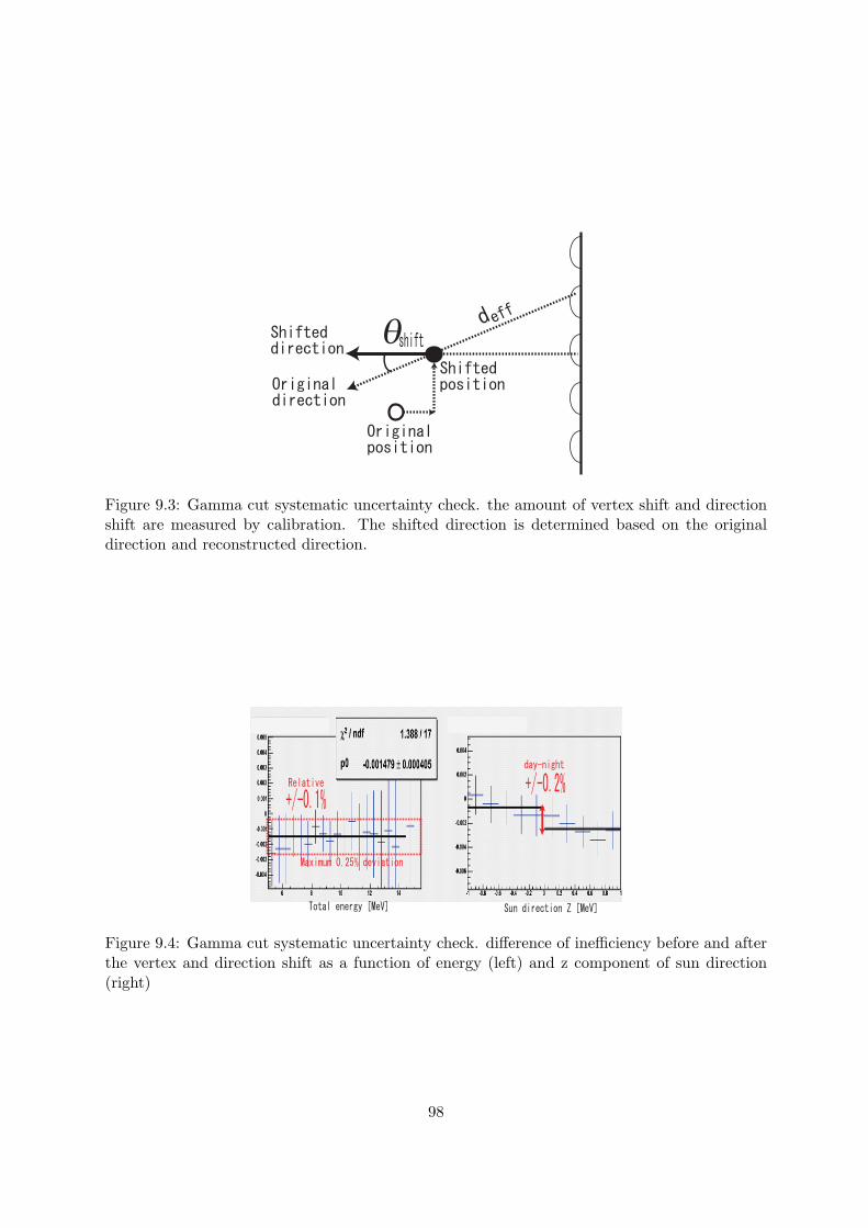
Figure 9.3: Gamma cut systematic uncertainty check. the amount of vertex shift and directionshift are measured by calibration. The shifted direction is determined based on the originaldirection and reconstructed direction.
Figure 9.4: Gamma cut systematic uncertainty check. difference of inefficiency before and afterthe vertex and direction shift as a function of energy (left) and z component of sun direction(right)
98
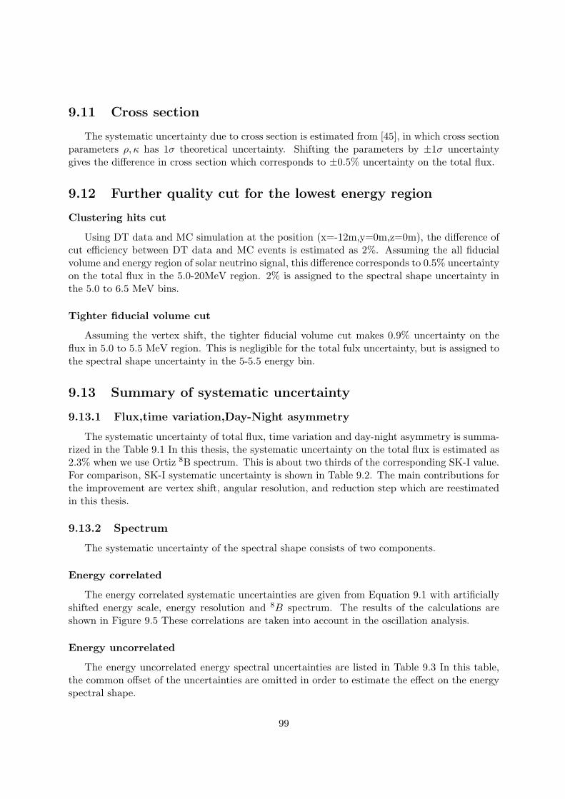
9.11 Cross section
The systematic uncertainty due to cross section is estimated from [45], in which cross sectionparameters ρ, κ has 1σ theoretical uncertainty. Shifting the parameters by ±1σ uncertaintygives the difference in cross section which corresponds to ±0.5% uncertainty on the total flux.
9.12 Further quality cut for the lowest energy region
Clustering hits cut
Using DT data and MC simulation at the position (x=-12m,y=0m,z=0m), the difference ofcut efficiency between DT data and MC events is estimated as 2%. Assuming the all fiducialvolume and energy region of solar neutrino signal, this difference corresponds to 0.5% uncertaintyon the total flux in the 5.0-20MeV region. 2% is assigned to the spectral shape uncertainty inthe 5.0 to 6.5 MeV bins.
Tighter fiducial volume cut
Assuming the vertex shift, the tighter fiducial volume cut makes 0.9% uncertainty on theflux in 5.0 to 5.5 MeV region. This is negligible for the total fulx uncertainty, but is assigned tothe spectral shape uncertainty in the 5-5.5 energy bin.
9.13 Summary of systematic uncertainty
9.13.1 Flux,time variation,Day-Night asymmetry
The systematic uncertainty of total flux, time variation and day-night asymmetry is summa-rized in the Table 9.1 In this thesis, the systematic uncertainty on the total flux is estimated as2.3% when we use Ortiz 8B spectrum. This is about two thirds of the corresponding SK-I value.For comparison, SK-I systematic uncertainty is shown in Table 9.2. The main contributions forthe improvement are vertex shift, angular resolution, and reduction step which are reestimatedin this thesis.
9.13.2 Spectrum
The systematic uncertainty of the spectral shape consists of two components.
Energy correlated
The energy correlated systematic uncertainties are given from Equation 9.1 with artificiallyshifted energy scale, energy resolution and 8B spectrum. The results of the calculations areshown in Figure 9.5 These correlations are taken into account in the oscillation analysis.
Energy uncorrelated
The energy uncorrelated energy spectral uncertainties are listed in Table 9.3 In this table,the common offset of the uncertainties are omitted in order to estimate the effect on the energyspectral shape.
99

Source Flux Time variation Day/Night
Energy scale ±1.4% ±1.3% ±1.3%Energy resolution ±0.2%8B spec. ±0.2/1.0%Trig. eff. ±0.5% ±0.1%Ang. resolution ±0.67%Vertex shift ±0.54%ReductionovaQ ±0.4%Hit pattern cut ±0.25%Second vertex ±0.45%Spallation ±0.2% ±0.1% ±0.1%Gamma-ray cut ±0.25% ±0.2%Cluster hit cut ±0.5%Background shape ±0.1% ±0.4%Signal ext. method ±0.7%Cross section ±0.5%
Total ±2.1/2.3% ±1.3% ±1.4%
Table 9.1: Summary of the total systematic uncertainty. The total value 2.1% is for Winter 8Bspectrum and 2.3% is for Ortiz
Source Flux Time variation Day/Night
Energy scale, resolution ±1.6% +1.2−1.1%
+1.2−1.1%
8B spec. ±1.0%Ang. resolution ±1.2%Vertex shift ±1.3%Reduction +2.1
−1.6%Spallation ±0.2% ±0.1% ±0.1%Gamma-ray cut ±0.5% ±0.25%Background shape ±0.1% ±0.4%Cross section ±0.5%Livetime calculation ±0.1% ±0.1% ±0.1%
Total +3.5−3.2% ±1.3% +1.3
−1.2%
Table 9.2: Summary of the total systematic uncertainty in SK-I.
100

Scale 0 .53%
R esolu tion 2 .5%
W in ter 06 B8 spec & err.
Scale 0 .53%
R esolu tion 2 .5%
Ortiz B8 spec,Bahcall err.
-0.15
-0.1
-0.05
0
0.05
0.1
0.15
4 6 8 10 12 14 16 18 20-0.15
-0.1
-0.05
0
0.05
0.1
0.15
4 6 8 10 12 14 16 18 20
Figure 9.5: Energy correlated systematic uncertainties for Ortiz (left) and Winter (right) 8Bspectrum.
Energy(MeV) 5-5.5 5.5-6 6-6.5 6.5-7 7-7.5 7.5-20
Trig eff ±2.4% ±0.9% ±0.1% - - -ovaQ ±2.% ±1.75% ±1.5% ±1.25% ±1.0% -Hit pat. - - - ±0.25% ±0.25% ±0.25%Cluster cut ±2.% ±2.% ±2.% - - -Gamma Cut ±0.1% ±0.1% ±0.1% ±0.1% ±0.1% ±0.1%Vertex shift ±0.5% ±0.1% ±0.1% ±0.1% ±0.1% ±0.1%BG shape ±0.2% ±0.8% ±0.2% ±0.2% ±0.2% ±0.2%Sig.Ext. ±2.1% ±0.7% ±0.7% ±0.7% ±0.7% ±0.7%Cross section ±0.2% ±0.2% ±0.2% ±0.2% ±0.2% ±0.2%
Total ±4.3% ±3.0% ±2.6% ±1.5% ±1.3% ±0.8%
Table 9.3: Energy uncorrelated systematic uncertainty on the spectrum shape.
101
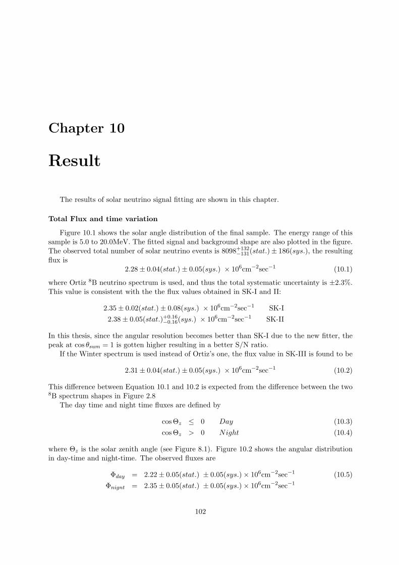
Chapter 10
Result
The results of solar neutrino signal fitting are shown in this chapter.
Total Flux and time variation
Figure 10.1 shows the solar angle distribution of the final sample. The energy range of thissample is 5.0 to 20.0MeV. The fitted signal and background shape are also plotted in the figure.The observed total number of solar neutrino events is 8098+132
−131(stat.)± 186(sys.), the resultingflux is
2.28 ± 0.04(stat.) ± 0.05(sys.) × 106cm−2sec−1 (10.1)
where Ortiz 8B neutrino spectrum is used, and thus the total systematic uncertainty is ±2.3%.This value is consistent with the the flux values obtained in SK-I and II:
2.35 ± 0.02(stat.) ± 0.08(sys.) × 106cm−2sec−1 SK-I2.38 ± 0.05(stat.)+0.16
−0.16(sys.) × 106cm−2sec−1 SK-II
In this thesis, since the angular resolution becomes better than SK-I due to the new fitter, thepeak at cos θsum = 1 is gotten higher resulting in a better S/N ratio.
If the Winter spectrum is used instead of Ortiz’s one, the flux value in SK-III is found to be
2.31 ± 0.04(stat.) ± 0.05(sys.) × 106cm−2sec−1 (10.2)
This difference between Equation 10.1 and 10.2 is expected from the difference between the two8B spectrum shapes in Figure 2.8
The day time and night time fluxes are defined by
cosΘz ≤ 0 Day (10.3)cosΘz > 0 Night (10.4)
where Θz is the solar zenith angle (see Figure 8.1). Figure 10.2 shows the angular distributionin day-time and night-time. The observed fluxes are
Φday = 2.22 ± 0.05(stat.) ± 0.05(sys.) × 106cm−2sec−1 (10.5)Φnignt = 2.35 ± 0.05(stat.) ± 0.05(sys.) × 106cm−2sec−1
102
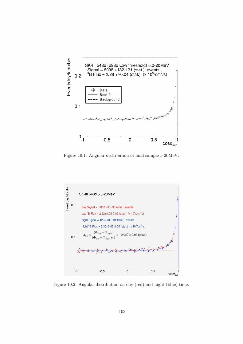
D ata
B est-fit
B ackground
Figure 10.1: Angular distribution of final sample 5-20MeV.
)stat.(031.0057.02/)(
)(±−=
Φ+Φ
Φ−Φ=
NightDay
NightDay
DNA
Figure 10.2: Angular distribution on day (red) and night (blue) time.
103

0
1
2
3
4
5
5 10 15 20
SK-III SLE 298d + LE 548d
Total energy of recoil electrons (MeV)
8 B F
lux
(106 /c
m2 /s
)
SK-III SLE 298d + LE 548d
Errors: stat. onlyLine: SK-III average
Figure 10.3: Energy spectrum of day(red) and night(blue). Black line shows SK-III average flux.
-0.2
-0.15
-0.1
-0.05
0
0.05
0.1
4 5 6 7 8 9 10
Figure 10.4: Day night asymmetry values as a function of energy threshold. The upper limit ofenergy is 20MeV.
104

Predicted
Figure 10.5: Time variation of observed flux. Green line shows the predicted value
The day-night asymmetry ADN is defined by
ADN =Φday − Φnight
12(Φday + Φnight)
(10.6)
= −0.057 ± 0.031(stat.) ± 0.013(sys)
The ADN in SK-I and II are:
ADN = −0.021 ± 0.020(stat.) +0.013−0.012(sys.) SK − I (10.7)
ADN = −0.63 ± 0.020(stat.) ± 0.037(sys.) SK − II
The ADN in SK-III is about 1.7σ away from 0, and the expected value from the oscillationparameters in favored Large Mixing Angle (LMA) solution is -1.5% [20]. To study this differencebetween ADN and 0, ADN values in the different energy regions are calculated, and it is confirmedthat those ADN values in the different energy regions are consistent with the 5-20MeV value (seeFigure ?? and 10.4). Further more, using the event sample before spallation cut above 6.5MeV(most events in a such sample are due to a single β ray which is emitted by spallation products ),it is also confirmed that energy scale of upward going events and that of downward going eventsare consistent within the assigned systematic uncertainty (±0.25%). Thus, any systematic biashas not been found to explain the large ADN value so far.
Figure 10.5 shows the time variation of observed solar neutrino flux. Each horizontal bincorresponds to 45 days. The correction of the elliptical orbit of the Earth is not taken intoaccount in this analysis. The fluctuation in SK-III seems large, but it would be statisticallyconsistent with the average value obtained by SK-I. Figure 10.6 shows the seasonal variation ofthe solar neutrino flux. The χ2 value is 13.6(d.o.f. = 7) which corresponds to 5.95% probability.(Cf. The χ2 value of SK-I is 4.7(d.o.f = 7) which corresponds to 69.9% probability.) Combining
105

Figure 10.6: Seasonal variation of observed flux. Solid line shows the predicted value from theelliptical orbit of the Earth.
106

Figure 10.7: Solar angle distributions of different energy regions from 4.5-7.5 MeV.
SK-I,II,and III statistically, the χ2 value is 3.6(d.o.f.=7) which corresponds to 89% probability.Thus, seasonal variation in SK-III is statistically consistent with SK-I.
Figure 10.7 shows the solar angle distribution in the different energy regions. The solar angledistribution in the 4.5-5MeV region is shown in the upper left plot. The background level isalmost the same as that of SK-I 5-5.5 MeV region (green histogram in middle top plot). Thesolar angle fitting result looks good, and the fitted number of signal events and the flux in the4.5-5MeV region are
4.5 − 5MeV : 232. ± 59.event (10.8)
and4.5 − 5MeV : 2.14+0.56
−0.54(stat.) × 106cm−2sec−1 (10.9)
This flux value is consistent with the 5-20MeV flux. Since the trigger efficiency in the SLE1period is not clear, the systematic uncertainty for this energy region was not estimated.
Energy spectrum
Figure 10.8 shows the expected and measured electron total energy spectrum. The expectedrate is calculated by the detector simulation which uses BP04 SSM. The solid line is expectedspectrum by SSM. The summary of observed and expected event rate is summarized in Table10.1. Figure 10.9 shows the ratio of observed energy spectrum to the SSM prediction. As shown
107
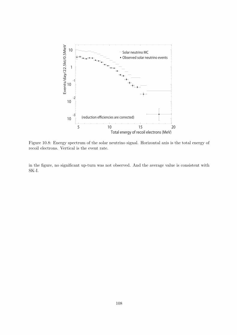
10-3
10-2
10-1
1
10
5 10 15 20Total energy of recoil electrons (MeV)
Ev
en
ts/d
ay
/22
.5k
t/0
.5M
eV
Solar neutrino MC
Observed solar neutrino events
(reduction e!ciencies are corrected)
Figure 10.8: Energy spectrum of the solar neutrino signal. Horizontal axis is the total energy ofrecoil electrons. Vertical is the event rate.
in the figure, no significant up-turn was not observed. And the average value is consistent withSK-I.
108

Ennergy (MeV) ALL DAY NIGHT 8B hep
5.0 − 5.5 64.4+8.0−7.7 73.2+12.2
−11.6 56.9+10.6−10.1 150.9 0.260
5.5 − 6.0 52.6+5.0−4.8 58.1+7.6
−7.2 47.6+6.6−6.2 138.2 0.250
6.0 − 6.5 49.1+3.8−3.7 43.2+5.4
−5.1 54.9+5.5−5.2 125.3 0.241
6.5 − 7.0 55.0+2.7−2.6 51.0+3.9
−3.7 58.7+3.8−3.7 140.4 0.289
7.0 − 7.5 53.7+2.5−2.4 55.5+3.6
−3.5 52.0+3.5−3.3 122.6 0.271
7.5 − 8.0 40.3+2.2−2.1 39.6+3.1
−3.0 41.0+3.1−2.9 106.5 0.257
8.0 − 8.5 36.5+1.9−1.8 37.3+2.7
−2.6 35.7+2.6−2.5 90.5 0.240
8.5 − 9.0 30.6+1.7−1.6 28.6+2.4
−2.2 32.7+2.4−2.3 75.6 0.223
9.0 − 9.5 22.4+1.4−1.3 19.8+1.9
−1.8 25.0+2.1−1.9 62.3 0.205
9.5 − 10.0 19.3+1.2−1.2 17.9+1.8
−1.6 20.7+1.8−1.7 50.0 0.186
10.0 − 10.5 14.4+1.0−1.0 15.1+1.5
−1.4 13.7+1.5−1.3 39.6 0.169
10.5 − 11.0 13.9+1.0−0.9 15.1+1.5
−1.3 12.9+1.3−1.2 30.6 0.151
11.0 − 11.5 9.54+0.80−0.74 9.59+1.20
−1.06 9.47+1.11−0.99 23.07 0.134
11.5 − 12.0 5.69+0.64−0.58 5.28+0.91
−0.77 6.11+0.96−0.82 17.07 0.118
12.0 − 12.5 4.96+0.57−0.51 4.16+0.80
−0.67 5.71+0.85−0.73 12.30 0.102
12.5 − 13.0 3.08+0.44−0.38 2.71+0.62
−0.50 3.44+0.66−0.54 8.60 0.088
13.0 − 13.5 1.95+0.36−0.30 1.61+0.48
−0.36 2.28+0.56−0.44 5.68 0.074
13.5 − 14.0 1.35+0.30−0.24 1.16+0.40
−0.28 1.51+0.48−0.36 3.78 0.062
14.0 − 15.0 2.19+0.36−0.31 2.06+0.53
−0.41 2.32+0.54−0.42 3.84 0.092
15.0 − 16.0 0.854+0.240−0.180 0.389+0.295
−0.162 1.249+0.398−0.284 1.326 0.059
16.0 − 20.0 0.115+0.134−0.066 0.248+0.242
−0.119 0.000+0.128−0.415 0.592 0.068
Table 10.1: Observed and expected rates in each energy bin at 1AU. The unit of the rate isevent/kton/year. The errors in the observed rate are statistical only. The reduction efficienciesare corrected, and the expected event rates are for the BP2004.
109
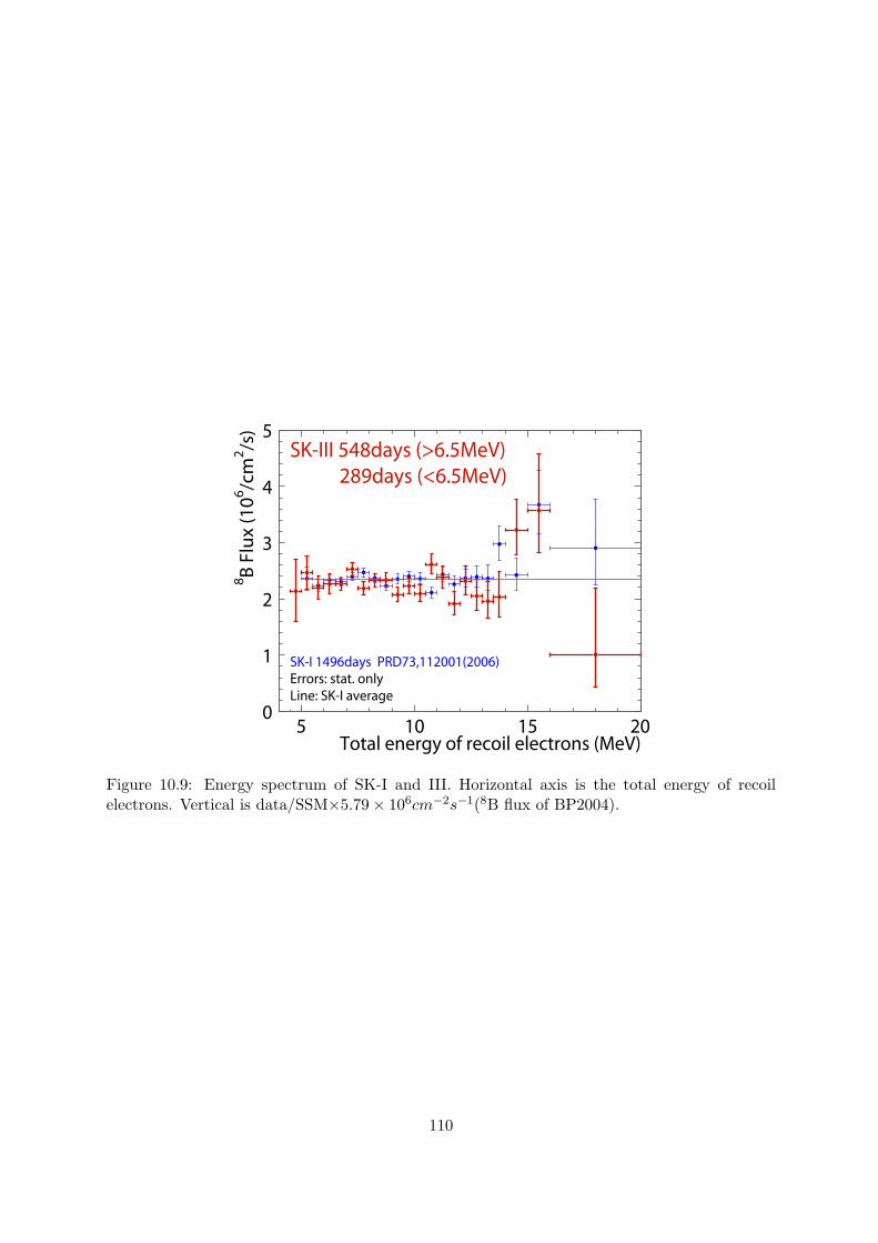
0
1
2
3
4
5
5 10 15 20
SK-I 1496days PRD73,112001(2006)
Total energy of recoil electrons (MeV)
8B
Flu
x (
10
6/c
m2/s
)
SK-III 548days (>6.5MeV)
289days (<6.5MeV)
Errors: stat. onlyLine: SK-I average
Figure 10.9: Energy spectrum of SK-I and III. Horizontal axis is the total energy of recoilelectrons. Vertical is data/SSM×5.79 × 106cm−2s−1(8B flux of BP2004).
110

Chapter 11
Oscillation Analysis
11.1 Spectrum fit
11.1.1 Spectrum shape prediction
The method to calculate the expected energy spectrum of the recoil electron by solar neutrinois following. Using the survival probability pe in Equation 2.23, the neutrino interaction rate inthe observed energy range Elow to Ehigh with the neutrino oscillation is written as
rosc =∫ Ehigh
Elow
dE
∫Eν
dEνϕ(Eν)∫
Ee
dEeR(Ee, E) (peSe(Eν , Ee) + (1 − pe)Sµ,τ (Eν , Ee)) (11.1)
where Se,µ,τ (Eν , Ee) describe the probability of the elastic scattering of a νe,x of energy Eν withan electron of recoil energy Ee. R(Ee, E) is the detector response function given by the equation9.2. ϕ(Eν) is the solar neutrino flux (8B or hep) as a function of neutrino energy. For the nulloscillation case, the rate rnull is given by setting pe = 1.
As described in Section 2.3, the pe consists of the Sun propagation part, p1, and the Earthpropagation part, p1e. Since we do not know the path of the observed neutrino in the Sun, p1
is obtained by averaging over the production points. On the other hand, for the earth part, ifthe event time and the position of the Sun and the detector at the time are given, a uniquepath of the observed neutrino can be calculated for an oscillation parameter set, (∆m2, θ), andeventually, pe is obtained as a function of neutrino energy (Eν) and zenith angle of the Sun,cz ≡ cosΘz, pe(Eν , cz). The interaction rate with the neutrino oscillation in Equation 11.1correspondingly has a form of rosc(E, cz).
In this analysis, cz of the night time (0 < cz ≤ 1) is divided into 1000 bins and 1 bin is forday time (−1 ≤ cz ≤ 0). With this binning, the interaction rate of 8B and hep neutrinos are
Bosc(E) =1001∑j=1
τ(czj)τtot
· r8Bosc(E, czj) (11.2)
Hosc(E) =1001∑j=1
τ(czj)τtot
· rheposc (E, czj) (11.3)
where τ(czj) is the livetime in the j-th zenith angle bin which is obtained from the real data(see Figure 11.1), and τtot is the total livetime. The predicted rate of the i-th bin ( Elow,i <
111
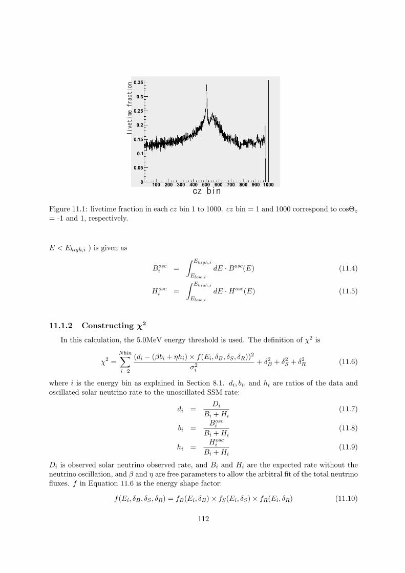
Figure 11.1: livetime fraction in each cz bin 1 to 1000. cz bin = 1 and 1000 correspond to cosΘz
= -1 and 1, respectively.
E < Ehigh,i ) is given as
Bosci =
∫ Ehigh,i
Elow,i
dE · Bosc(E) (11.4)
Hosci =
∫ Ehigh,i
Elow,i
dE · Hosc(E) (11.5)
11.1.2 Constructing χ2
In this calculation, the 5.0MeV energy threshold is used. The definition of χ2 is
χ2 =Nbin∑i=2
(di − (βbi + ηhi) × f(Ei, δB, δS , δR))2
σ2i
+ δ2B + δ2
S + δ2R (11.6)
where i is the energy bin as explained in Section 8.1. di, bi, and hi are ratios of the data andoscillated solar neutrino rate to the unoscillated SSM rate:
di =Di
Bi + Hi(11.7)
bi =Bosc
i
Bi + Hi(11.8)
hi =Hosc
i
Bi + Hi(11.9)
Di is observed solar neutrino observed rate, and Bi and Hi are the expected rate without theneutrino oscillation, and β and η are free parameters to allow the arbitral fit of the total neutrinofluxes. f in Equation 11.6 is the energy shape factor:
f(Ei, δB, δS , δR) = fB(Ei, δB) × fS(Ei, δS) × fR(Ei, δR) (11.10)
112

wherefx(Ei, δx) =
11 + δx × ϵ±x (Ei)
, (x = B,S,R) (11.11)
and B,S, R denote the 8B spectrum, energy scale, energy resolution, respectively. δx is the unit-less parameter to scale the energy correlated uncertainty, ϵ±x (Ei) in Figure 9.5. The δx is varieduntil the χ2 gives the minimum value with βm and ηm. βm and ηm are calculated analyticallyby setting the partial first derivative of χ2 with respect to β and η to zero.
σi in equation 11.6 is combined statistical-systematic uncertainty, in which the energy un-correlated systematic uncertainties are combined in quadrature with the energy spectrum’s sta-tistical uncertainties. To account for the total flux energy uncorrelated systematic uncertainty,Taylor expanding of χ2 is carried out around the χ2 minimum (χ2
m) with:
χ2(β, η) = χ2m(βm, ηm) +
(β − βm
η − ηm
)T
C0
(β − βm
η − ηm
)(11.12)
where C0 is
C0 =Nbin∑i=2
b2iσ2
i
bihi
σ2i
bihi
σ2i
h2i
σ2i
(11.13)
Then C0 is scaled by αsys to add the total energy uncorrelated systematic uncertainty σsys. αsys
is defined as
αsys =σ2
0
σ20 + σ2
sys
, where σ20 =
Nbin∑i=2
1σ2
i
(11.14)
σsys is obtained as the total flux × (energy uncorrelated sys. on the total flux) / SSM flux,which is 2.28 ×
√0.0232(total) − 0.0142(escale) − 0.0022(eres.) − 0.012(8B)/5.79 = 0.6% for
SK-III. Then, the χ2 becomes
χ2α,SK3(β, η) = χ2
m(βm, ηm) +
(β − βm
η − ηm
)T
αsys · C0
(β − βm
η − ηm
)(11.15)
The χ2 for the energy spectrum shape is eventually expressed as: excluded
χ2specSK3(β, η) = Min(χ2
α,SK3(β, η, δB, δS , δR) + δ2B + δ2
S + δ2R) (11.16)
where the number of fitting parameters is five; β, η, δB, δS , δR. Inside of line is excluded. Figure11.2-(a) shows the exclude region by the SK-III spectrum obtained from the Equation 11.16.
11.2 Time-Variation Analysis
In the time-variation analysis, 6.5MeV energy threshold is used. In order to take into accountthe time variation of the rate due to the matter effects of the Earth, the sij of Equation 8.1 ismodified with a scaling function ri(tj)/rave
i . Here, tj is the event time of the j-th event andri(tj) is the predicted time dependence (that is, cz dependence) of the expected oscillated solar
113
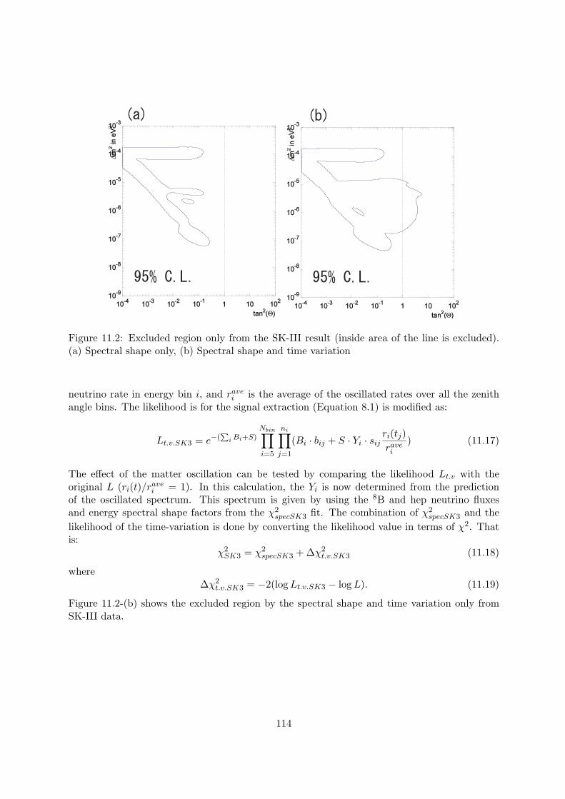
Figure 11.2: Excluded region only from the SK-III result (inside area of the line is excluded).(a) Spectral shape only, (b) Spectral shape and time variation
neutrino rate in energy bin i, and ravei is the average of the oscillated rates over all the zenith
angle bins. The likelihood is for the signal extraction (Equation 8.1) is modified as:
Lt.v.SK3 = e−(∑
i Bi+S)Nbin∏i=5
ni∏j=1
(Bi · bij + S · Yi · sijri(tj)ravei
) (11.17)
The effect of the matter oscillation can be tested by comparing the likelihood Lt.v with theoriginal L (ri(t)/rave
i = 1). In this calculation, the Yi is now determined from the predictionof the oscillated spectrum. This spectrum is given by using the 8B and hep neutrino fluxesand energy spectral shape factors from the χ2
specSK3 fit. The combination of χ2specSK3 and the
likelihood of the time-variation is done by converting the likelihood value in terms of χ2. Thatis:
χ2SK3 = χ2
specSK3 + ∆χ2t.v.SK3 (11.18)
where∆χ2
t.v.SK3 = −2(log Lt.v.SK3 − log L). (11.19)
Figure 11.2-(b) shows the excluded region by the spectral shape and time variation only fromSK-III data.
114

Figure 11.3: Excluded region from the SK combined analysis (inside area of the line is excluded).Black shows only SK-I and II, Red shows SK-I,II and III. (a) Spectral shape only . (b) Spectralshape and time variation.
11.3 Oscillation constraint from SK
The combined χ2 to be minimized is following:
χ2specSK = Min(χ2
α,SK1(β, η, δB, δS1, δR1)
+χ2α,SK2(β, η, δB, δS2, δR2)
+χ2α,SK3(β, η, δB, δS3, δR3)
+δ2B + δ2
S1 + δ2R1 + δ2
S2 + δ2R2 + δ2
S3 + δ2R3) (11.20)
where the energy threshold is 5.0MeV (i=2 to 22) for SK-I and 7.0MeV (i=6 to 22)for SK-II[46]. In Equation 11.20, seven parameters are fitted. The full SK χ2 is obtained by adding thetime variation terms in each phase.
χ2SKfull = χ2
specSK + ∆χ2t.v.SK1 + ∆χ2
t.v.SK2 + ∆χ2t.v.SK3 (11.21)
Figure 11.3 show the exclusion region obtained from the spectral fit (a), and the spectral fit plusthe time variation (b).
115
Chapter 12
Discussion
12.1 Global oscillation analysis
The combined analysis of other solar neutrino experiments and KamLAND experiment isdiscussed in this section. The numbers which are used in this global analysis are based on theresults summarized in Section ??.
12.1.1 SNO
The results of the CC total flux measured by D2 O phase(CC) and salt phase(CC) areincluded in this thesis. For the NC flux, the latest low-energy threshold analysis (LETA) [47] isalso included. The latest value of NC flux is
ΦNC = 5.14+0.160−0.158(stat.)+0.132
−0.117(sys.) × 106cm−2s−1 (12.1)
This represents 3.1% statistical uncertainty and 2.4% systematic uncertainty.The definition of χ2 is following:
χ2SNO =
(DSNO1CC − (βBSNO1
CC + ηHSNO1CC ))2
(σSNO1CC )2
+(DSNO2
CC − (βBSNO2CC + ηHSNO2
CC ))2
(σSNO2CC )2
+(DNC − (βBSSM + ηHSSM ))2
(σNC)2+
(ADNCC − ADNpred(β, η))2
(σADNCC)2
(12.2)
where ADNpred(β, η) is the predicted day-night asymmetry parameter of pure D2O phase:
ADNpred(β, η) = 2 ×(βBSNO1,day
CC + ηHSNO1,dayCC ) − (βBSNO1,night
CC + ηHSNO1,nightCC )
(βBSNO1,dayCC + ηHSNO1,day
CC ) + (βBSNO1,nightCC + ηHSNO1,night
CC )(12.3)
The combined χ2 to be minimized is then given:
χ2SK+SNO(β, η) = χ2
specSK(β, η) + χ2SNO(β, η) (12.4)
The common flux scale factors are used in this calculation. So, the number of fitted parametersare 7, same as in Equation 11.20.
116
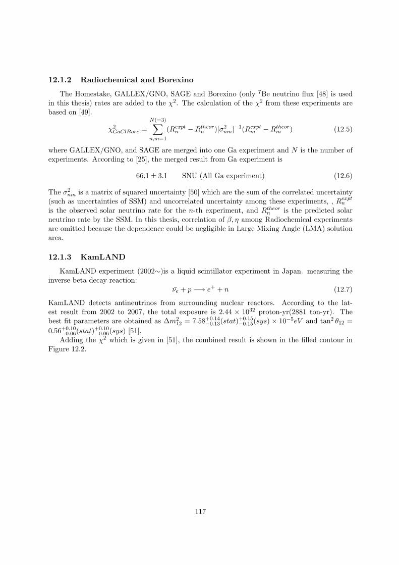
12.1.2 Radiochemical and Borexino
The Homestake, GALLEX/GNO, SAGE and Borexino (only 7Be neutrino flux [48] is usedin this thesis) rates are added to the χ2. The calculation of the χ2 from these experiments arebased on [49].
χ2GaClBore =
N(=3)∑n,m=1
(Rexptn − Rtheor
n )[σ2nm]−1(Rexpt
m − Rtheorm ) (12.5)
where GALLEX/GNO, and SAGE are merged into one Ga experiment and N is the number ofexperiments. According to [25], the merged result from Ga experiment is
66.1 ± 3.1 SNU (All Ga experiment) (12.6)
The σ2nm is a matrix of squared uncertainty [50] which are the sum of the correlated uncertainty
(such as uncertainties of SSM) and uncorrelated uncertainty among these experiments, , Rexptn
is the observed solar neutrino rate for the n-th experiment, and Rtheorn is the predicted solar
neutrino rate by the SSM. In this thesis, correlation of β, η among Radiochemical experimentsare omitted because the dependence could be negligible in Large Mixing Angle (LMA) solutionarea.
12.1.3 KamLAND
KamLAND experiment (2002∼)is a liquid scintillator experiment in Japan. measuring theinverse beta decay reaction:
ν̄e + p −→ e+ + n (12.7)
KamLAND detects antineutrinos from surrounding nuclear reactors. According to the lat-est result from 2002 to 2007, the total exposure is 2.44 × 1032 proton-yr(2881 ton-yr). Thebest fit parameters are obtained as ∆m2
12 = 7.58+0.14−0.13(stat)+0.15
−0.15(sys) × 10−5eV and tan2 θ12 =0.56+0.10
−0.06(stat)+0.10−0.06(sys) [51].
Adding the χ2 which is given in [51], the combined result is shown in the filled contour inFigure 12.2.
117

2521.1
67.1
2
21
024.0
011.012
2
eV 1003.6
29.0sin
−+
−
+
−
×=∆
=
m
θ
Figure 12.1: Allowed region of LMA (inside area of the line is allowed)
2512.0
39.0
2
21
017.0
016.012
2
eV 1059.7
304.0sin
−+
−
+
−
×=∆
=
m
θ
This result
KamLAND
Solar
Figure 12.2: Allowed region of LMA, Solar + KamLAND (inside area of the line is allowed)
118

0
1
2
3
4
5
5 10 15 20Total energy of recoil electrons (MeV)
8B
Flu
x (1
06/c
m2/s
)
Errors: stat. onlyLine: SK-I average
Figure 12.3: SK-III data /SSM (BP2004) with Winter and Ortiz 8B spectrum. Green showsSSM with Winter 8B spectrum, and red shows SSM with Ortiz 8B spectrum.
12.2 Comparison of Winter and Ortiz 8B spectrum
In this section, the effect of the difference between Winter 8B spectrum and Ortiz 8B spec-trum to the oscillation contour is discussed.
Figure 12.3 shows the SK-III energy spectra divided by SSM with Winter 8B spectrum andOrtiz 8B spectrum. Since the Ortiz spectrum has more tail in the higher energy region comparedto the Winter spectrum (see Figure 2.8), the energy spectrum over the SSM prediction becomeslarger in high energy region if the Winter spectrum is used for the SSM prediction. Therefore,if the Wineter spectrum is used, this makes the χ2 value of the spectrum fitting worse in theLMA solution area because the LMA predicts upturn of the energy spectrum in the lower energyregion, and thus, the LMA area is excluded slightly lager. In Figure 12.4, we can see this effect.For the spectrum fitting, I use different energy correlated systematic uncertainties for Winterand Ortiz spectrum which are shown in Figure 9.5.
12.3 Comparison with other results
Figure 12.5 shows the comparison of the results on the mixing angle measurements. Thereason why only the mixing angle results are compared is that the uncertainty of ∆m2 is mainlycontrolled by KamLAND, and thus, for the solar neutrino experiments, the contribution to the∆m2 measurement is smaller than the contribution to the mixing angle measurement. As shownin Figure 12.5, even though only the CC and NC rate information from SNO are used in thisthesis, the size of uncertainty is about the same. This indicates that if more information ofthe SNO results, for example CC spectral shape, is added to the SK result, the global analysisresults will be improved.
Using these oscillation parameters obtained from the solar and reactor experiments, the fluxvalue of 8B neutrino can be extracted. As in Equation 11.20, the β is a free parameter tominimize the χ2
SK+SNO and there is no constraint from the SSM prediction in the χ2SK+SNO.
119

∆m
2 in e
V2
10-9
10-8
10-7
10-6
10-5
10-4
10-3
tan2(Θ)10-4 10-3 10-2 10-1 1 10 102
∆m
2 in e
V2
10-9
10-8
10-7
10-6
10-5
10-4
10-3
tan2(Θ)10-4 10-3 10-2 10-1 1 10 102
Winter B spectrumOrtiz B spectrum8
8
95% C.L
LMA
Figure 12.4: Excluded region by SK-III data /SSM (BP2004) with Winter and Ortiz 8B spec-trum shapes. Green shows SSM with Winter 8B spectrum, and red shows SSM with Ortiz 8Bspectrum.
120

26
28
30
32
34
36
38
40
θ12
[deg
.]
SN
O-I,
II,S
L
SN
O-I,
II, S
L+K
L
SN
O-I,
II,III
, SL+
KL
SN
O-II
I,LE
TA, S
L+K
L
SK
-I,II,
III,S
L+ K
L
3fla
vor (
T.S
chw
etz)
Figure 12.5: Comparison of the mixing angle measurement between SNO results and the resultsobtained by this thesis. the error size corresponds to 1 σ uncertainty of (stat.+sys.). SNO-I,II,SL use SNO phase I and II and other solar neutrino data (SL) [29] and SNO-I,II,SL+KLadded KamLAND(2004) [29]. SNO-I,II,III,SL+KL add the phase III [30] and updated Kam-LAND(2008) [51]. SNO-III,LETA+KL is latest SNO result [47]. Result of this work is shownas SK-I,II,III SL+KL. The 3 flavor analysis is from the analysis of latest solar + reactor+atmospheric results [52]
Thus, the flux value scaled by the βm does not depend on the SSM so much. Figure 12.6 showsthe scaled 8B flux values by using the βm at the best fit point obtained by the global solaranalysis and the global solar + KamLAND analysis and they are compared with the 8B fluxobtained by SNO NC rate. The size of error corresponds to the maximum and minimum fluxvalues among the 1σ oscillation parameter region. The obtained 8B flux values are;
Global solar analysis: 5.27+0.16−0.13 × 106cm−2s−1
Global solar+KamLAND analysis: 5.08+0.10−0.07 × 106cm−2s−1
As shown in Figure 12.6, the flux obtained by the solar neutrino experiments agree with the allthe SSM predictions (BP04, BS05(OP) and BS05(AGS,OP)), and the seismic model prediction[7] within their uncertainties. However, the size of the experimental uncertainty (∼ 2%)is muchsmaller than that of SSMs. Thus, our results of 8B flux measurement can be a strong tool totest the future improvement of SSM.
121

4
4.5
5
5.5
6
6.5
7
7.5
8
8.5
SN
O-II
I
SN
O-L
ETA
Sol
ar G
loba
l (Th
is w
ork)
Sol
ar+K
amLA
ND
(Thi
s w
ork)
B F
lux
[X10
cm
sec
]8
6
-2
-
1
SN
O-II
SN
O-I
Figure 12.6: Comparison of the 8B flux between SNO results and the results obtained by this the-sis. the error size corresponds to 1 σ uncertainty of (stat.+sys.). Square mark shows theoreticalpredictions and cross marks shows experimental results.
12.4 Treat reduction uncertainties as energy correlated uncer-tainties
In Chapter 9, the uncertainties of ambient cuts (ovaQ cut and hit pattern cut) are treated asenergy uncorrelated uncertainty. However, if MC simulation gives systematically better goodnessthan the real data, for example, the uncertainties for each energy bins move to the same direction.That is, the uncertainties of ambient cuts have some energy correlation. To estimate how thisenergy correlation affects the fitting of the spectrum, those uncertainties (ovaQ cut and hitpattern cut) are treated as energy correlated uncertainties here.
Figure 12.7 shows the uncertainties of ovaQ cut and hit pattern cut which are obtained fromthe comparisons between LINAC data and MC simulation (see Figure 9.1 and 9.2 of Section9.6). These uncertainties are assigned as ±1σ uncertainties of the ambient cut efficiency (seethe purple histogram of Figure 7.21), and treated as ϵ±x of Equation 11.11. Hence, the definitionin χ2
specSK3 of Equation 11.16 becomes
χ2specSK3(β, η) = Min(χ2
α,SK3(β, η, δB, δS , δR, δovaQ, δHitPat) + δ2B + δ2
S + δ2R + δ2
ovaQ + δ2HitPat)
(12.8)where the free parameters to be fitted are β, η, δB, δS , δR, δovaQ, δHitPat. To avoid double countingof uncertainties, the energy uncorrelated systematic uncertainties are modified as in Table 12.1.
By taking them as energy correlated uncertainties, all data points shift to the same directionwhen they are fitted. This treatment gives a slightly tighter allowed region than when the datapoints are uncorrelated (see Figure 12.8). The best-fit point is unchanged after this modification.
122

-5
-4
-3
-2
-1
0
1
2
3
4
5
6 8 10 12 14 16 18 20
Figure 12.7: Energy correlated systematic uncertainties of ovaQ and hit pattern cut.
Energy(MeV) 5-5.5 5.5-6 6-6.5 6.5-7 7-7.5 7.5-20
Total ±3.8% ±2.4% ±2.1% ±0.8% ±0.8% ±0.8%
Table 12.1: Energy uncorrelated systematic uncertainty on the spectrum shape. The contribu-tions from ovaQ and Hit pattern cut are removed from Table 9.3
123

∆m
2 i
n e
V2
10-9
10-8
10-7
10-6
10-5
10-4
10-3
tan2(Θ)
10-4
10-3
10-2
10-1
1 10 102
∆m
2 i
n e
V2
x10-4
0
1
2
sin2(Θ)
0.0 0.1 0.2 0.3 0.4 0.5 0.6 0.7 0.8 0.9 1.0
∆m
2 i
n e
V2
x10-4
0
1
2
sin2(Θ)
0.0 0.1 0.2 0.3 0.4 0.5 0.6 0.7 0.8 0.9 1.0
Figure 12.8: Excluded region (inside area of blue line) from SK-III spectrum fit (left) and allowedregion from all solar neutrino experiments (right). The systematic uncertainties of ambient cutare treated as energy correlated uncertainties. Black line in left plot shows the result in whichthe uncertainties have no correlation. The best fit point of global analysis is not changed whetherthe uncertainties are energy correlated or not.
124
0
0.1
0.2
0.3
0.4
0.5
0.6
0.7
0.8
6 8 10 12 14 16 18 20
Figure 12.9: SK-III spectrum with expected distorted shapes and flat shape. The error showsonly statistical uncertainty.
Even if this treatment gives better results, it is not clear how much the uncertainty band shownin Figure 12.7 is energy correlated. Thus, in the final results on parameter region of solarneutrino oscillation, the uncertainties of the ambient cuts are treated as energy uncorrelatedconservatively.
12.5 Sensitivity to upturn
Figure 12.9 shows SK-III energy spectrum with solar best fit, solar plus KamLAND bestfit, and flat expectations. The χ2 value with each case is following: 26.8/20d.o.f. (solar bestfit: ∆m2 = 6.03 × 10⁻⁵eV 2, sin2 θ = 0.29), 26.7/20d.o.f. (solar plus KamLAND best fit:∆m2 = 7.59 × 10⁻⁵eV 2, sin2 θ = 0.34), and 27.7/20d.o.f. (flat shape). When the ambient cutuncertainties are treated as energy correlated systematic uncertainty, the χ2 value with eachcase is following: 26.9/20d.o.f. (solar best fit), 27.0/20d.o.f. (solar plus KamLAND best fit),and 27.5/20d.o.f. (flat shape).
Figure 12.10 shows spectral shape of each phase with solar best fit expectation. Although itis not statistically significant, the spectral shape of SK-III might show a little hint of the upturn.
Finally, a sensitivity of the observation of upturn is estimated. Followings are assumed forthis estimation;
1. Background level is same as SK-III.
2. Energy correlated systematic uncertainty is half of SK-I
3. 4 MeV threshold is accomplished.
125

5 15 10
0.1
0.2
0.3
0.4
0.5
0.6
0.7
0.8
5 10 15 20 0 15 20 0 15 20
Figure 12.10: SK-I,II, and III spectrum with expected distorted shapes and flat shape. Theerror shows only statistical uncertainty.
126

If we use Winter06 8B spectrum, energy correlated uncertainty of SK-III already achieves 30%improvement since SK-I. Further 20% improvement would be possible if the position and di-rection dependence of energy scale becomes half of current dependence. This is done by moreprecise calibrations and a better modeling of water condition. Item 3 would be possible be-cause the new electronics and DAQ system, which are already installed in 2008, can store allhit information without hardware trigger. Under this assumption, about 2σ level observationwithin 3 years, and about 3σ level within 10 years could be expected. In addition to new data,re-analysis of SK-I data is desirable because the calibration method and analysis tools whichare developed in this thesis can be applied to SK-I data and expected to reduce uncertainties.Since we already have 6 years of total livetime during SK-I and III, A 3σ level discovery of theupturn might be possible within few years if the SK-I data are re-analyzed.
127
Chapter 13
Conclusion
In conclusion, the measurement of solar neutrino with SK-III was carried out aimed at theobservation of the spectrum distortion due to MSW effect. The strategies of this thesis to achievethis goal are to reduce the background level by 70% from SK-I in the lower-energy region, andto reduce the energy correlated systematic uncertainty by 50% compared to SK-I.
With improved detector calibrations, a full detector simulation, and analysis methods, thenumber of background events is reduced by about 50% from SK-I. Meanwhile, the energy cor-related systematic uncertainties are reduced by 30%, and the energy uncorrelated systematicuncertainties are reduced by 60% from SK-I. Thus, the goal is almost achieved and acceptablefor the future observation of the spectrum distortion.
The systematic uncertainty of the total flux is estimated as ±2.3%, and is about two thirdof SK-I. The 8B flux in SK-III is
2.28 ± 0.04(stat.) ± 0.05(sys.) × 106cm−2sec−1
which is the most precise result of previous results from SK-I and II. A day-night asymmetry isobtained to be
ADN = −0.057 ± 0.031(stat.) ± 0.013(sys.)
After combining the previous phase of SK and other solar neutrino experiments, the best-fitparameters of the solar neutrino oscillation are determined with the world’s best accuracy;
sin2 θ12 = 0.29+0.024−0.011
∆m212 = 6.03+1.21
−1.67 × 10⁻⁵eV 2
By adding the result from KamLAND, the obtained best-fit parameters are
sin2 θ12 = 0.304+0.017−0.016
(θ12 = 33.46+1.05−1.00)
∆m221 = 7.59+0.12
−0.39 × 10⁻⁵eV 2
which are consistent with the latest analysis by SNO group.The χ2 value of spectrum fit with the solar plus KamLAND best-fit prediction is 26.7/20d.o.f.
which is slightly better than 27.7/20d.o.f. with a flat shape. Although, this result is notstatistically significant, it is estimated that the improved calibration and analysis methods willgive a sensitivity of 3σ level discovery of the spectrum distortion within a few years, togetherwith re-analysis of the SK-I data.
128

Appendix A
Glossary
ADC Analog to Digital Converter
ATM Analog Timing Module; front end electronics based on TKO standard.
BP04 One of the SSM series published in 2004, which is used in this thesis.
BONSAI Branch Optimization Navigating Succesive Annealing Iterations, the standard vertexfitter for this analysis.
BS05(AGS,OP) One of SSM series published in 2005, which uses the latest physics informa-tion, called the ”low Z” model including updated opacity calculation by Opacity Project.
BS05(OP) One of SSM series published in 2005, which used the previous heavy metal abun-dance, called the ”high Z” model. Other updates including the opacity calculation by OPare implemented.
COREPMT Average Q.E. determined by LINAC 8.8MeV. This in one of input parametersfor MC
DT Duteron Tritium generator (neutron source)
HE High Energy Trigger (-320mV)
HITSUM summation of hit square pulses
ID Inner Detector
LMA Large Mixing Angle solution of solar neutrino oscillation
LE trigger Low Energy trigger (-302mV)
LINAC LINear ACcelerator
LMA Large Mixing Angle solution of the solar neutrino oscillation. 10−5 < ∆m2 < 10−4eV2
and θ12 ∼ 30 − 40◦
Neff Effective number of hits in a event.
Nhit The number of hits in one event.
129

Ni calibration Calibration using Cf-Ni gamma-ray source
Nx The number of hits within x nsec time window. The number is found after applying thesliding x nsec time-window search to the t − tof − t0 distribution.
OD Outer Detector
ovaQ One dimensional variable for Vertex and Angular Quality: G2V − G2
A
PMT Photo Multiplier Tube
QAC Charge to Analog Converter
Q.E. Quantum efficiency of PMT
Seismic model One of solar models. This model is based on a standard stellar evolution andthe input information is adjusted for the Sun by the seismic measurements.
S-factor Cross section factor of nuclear fusion reactions in the Sun.
SLE1 trigger Super Low Energy trigger period 1(-212mV)
SLE2 trigger Super Low Energy trigger period 2(-186mV)
SMP Super Meory Partner; VME memory modules after ATM
Spallation cut Cut to reject sapallation products
SSM the Standard Solar Model. A series of solar model first developed by J.N.Bahcall.
TAC Timing to Analog Converter
TBA Top Bottom Asymmetry of the detector
Tisk hit timing of each PMT (without subtruction of TOF)
TKO Tristan KEK Online standard
TOF Time of flight
TQmap Hit timing correction function as a fuction of charge
TRG TRiGger module which distribute the global trigger and the event number
130

Bibliography
[1] Z. Maki et al. Phys.Lett. 28B 498 (1969)
[2] L. Wolfenstein Phys.Rev.D 17 2369 (1978)
[3] S. P. Mikheyev and A. Yu. Smilnov Nuovo Cim. 9C 17 (1986)
[4] J. N. Bahcall Neutrino Astrophysics Cambridge University Press (1989)
[5] J. N. Bahcall et al. Phys.Lett,B 374 1 (1996)
[6] H. Bethe Phys.Rev., 55 434 (1939)
[7] Turck-Chieze et al. Phys.Rev.Lett. 93 211102 (2004)
[8] J. N. Bahcall et al. Phys.Rev.Lett., 92 121301 (2004)
[9] J. N. Bahcall et al. Astrophys.J, 621 83 (2005)
[10] A. M. Serenelli Nucl.Phys.B (Proc.Suppl.), 168 115 (2005)
[11] M. Asplund et al. Nucl.Phys.A 777 1 (2005)
[12] N. Grevesse et al. Space.Sci.Rev., 85 161 (1998)
[13] N. R. Badnell et al. MNRAS, 360 458 (2005)
[14] C. A. Iglesias Astrophys.J., 464 943 (1996)
[15] A. M. Serenelli Astrophys.J., 705 123 (2009)
[16] D. L. Anderson, Theory of the Earth Blackwell scientific publication (1989)
[17] C. E. Ortiz et al. Phys.Rev.Lett., 85 2909 (2000)
[18] J. N. Bahcall et al. Phys.Rev.C 54 411 (1996)
[19] W. T. Winter et al. Phys.Rev.C, 73 025503 (2006)
[20] J. Hosaka et al. (Super-Kamiokande Collaboration) Phys.Rev.D, 73 112001 (2006)
[21] Phys.Rev.Lett D 62 113004 (2000)
[22] B. T. Cleveland et al. Astrophys.J., 496 505 (1998)
131

[23] W. Hampel et al. Phys.Lett.B 447 127 (1999)
[24] M. Altmann et al. Phys.Lett.B 616 174 (2005)
[25] T. J. Bowles arXiv:0901.2200v1
[26] Y. Fukuda et al, Phys.Rev.Lett 77 420 (1998)
[27] C. Arpesella et al. Phys.Lett. B658 101 (2008)
[28] Q. R. Ahmad et al. Phys.Rev.Lett. 89 011301 (2002)
[29] B. Aharmim et al. Phys.Rev. C72 055502 (2005).
[30] B Ahrmim et al. Phys.Rev.Lett 101 111301 (2008)
[31] S. Fukuda et al. Nucl.Instr.and Meth. A 51 (2003) 418
[32] http://sales.hamamatsu.com/assets/pdf/parts R/R3600-06.pdf
[33] H. Ikeda et al. Nucl.Inst.and Meth. A 320 310 (1992)
[34] T. Tanimori et al. IEEE Trans.Nucl.Sci NS-36 497 (1989)
[35] T. K. Ohsuka et al. KEK Report 85-10 (1985)
[36] M. Smy Proc. of the 30th ICRC, 5 1279 (2007)
[37] ”GEANT - Detector Description and Simulation Tool”, CERN Program Library (1993)
[38] Y. Koshio Ph.D thesis, University of Tokyo, ICRR-Report-426-98-22 (1998)
[39] R. M. Pops et al. Applied Optics 35 33 (1997)
[40] E. Blaufuss et al. Nucl.Instr.and Meth. A 458 636 (2001)
[41] W. Y. Chang et al. Nature 139 962 (1937)
[42] M. Nakahata et al. Nucl.Instr.and Meth. A 421 113 (1999)
[43] L. Lyons, Statistics for nuclear and particle physicists Cambridge University Press, Cam-bridge
[44] E. Commins and P. H. Bucksbaum Weak interactions of leptons and quarks CambridgeUniversity Press, Cambridge
[45] J. N. Bahcall et al. Phys.Rev.D 51 6416 (1995)
[46] J. P. Cravens Phys.Rev.D 78 032002 (2008)
[47] B. Aharmim et al. arXiv:0910.2984v1 (2009)
[48] E. A. Litvinovich Phys.Atom.Nucl. 72 522 (2009)
[49] G. L. Fogli et al. Phys.Rev.D 66 05310, arXiv:hep-ph/0206162v1 (2002)
132

[50] G. L. Fogli et al. PHys.Rev.D 62 013002
[51] S. Abe et al. Phys.Rev.Lett. 100 221803 (2008)
[52] T. Schwetz et al. New Journal of Physics 10 113011 (2008)
133