First measurement of pp neutrinos in

real time in the Borexino detector

Pablo Mosteiro

A Dissertation

Presented to the Faculty

of Princeton University

in Candidacy for the Degree

of Doctor of Philosophy

Recommended for Acceptance

by the Department of

Physics

Adviser: Cristiano Galbiati

September 2014

© Copyright by Pablo Mosteiro, 2014.

All rights reserved.

Abstract

The Sun is fueled by a series of nuclear reactions that produce the energy that makes

it shine. Neutrinos (ν) produced by these nuclear reactions exit the Sun and reach

Earth within minutes, providing us with key information about what goes on at the

core of our star. For over twenty years since the first detection of solar neutrinos in

the late 1960’s, an apparent deficit in their detection rate was known as the Solar

Neutrino Problem. Today, the Mikheyev-Smirnov-Wolfenstein (MSW) effect is the

accepted mechanism by which neutrinos oscillate inside the Sun, arriving at Earth

as a mixture of νe, νµ and ντ , the latter two of which were invisible to early detec-

tors. Several experiments have now confirmed the observation of neutrino oscillations.

These experiments, when their results are combined together, have demonstrated that

neutrino oscillations are well described by the Large Mixing Angle (LMA) solution of

the MSW effect.

This thesis presents the first measurement of pp neutrinos in the Borexino de-

tector, which is another validation of the LMA-MSW model of neutrino oscillations.

In addition, it is one more step towards the completion of the spectroscopy of pp

chain neutrinos in Borexino, leaving only the extremely faint hep neutrinos unde-

tected. This advance validates the experiment itself and its previous results. This is,

furthermore, the first direct real-time measurement of pp neutrinos. We find a pp neu-

trino detection rate of 143±16 (stat)±10 (syst) cpd/100 t in the Borexino experiment,

which translates, according to the LMA-MSW model, to (6.42±0.85)×1010 cm−2 s−1.

We also report on a measurement of neutrons in a dedicated system within the

Borexino detector, which resulted in an improved understanding of neutron rates

in liquid scintillator detectors at Gran Sasso depths. This result is crucial to the

development of novel direct dark matter detection experiments.

iii

Acknowledgements

The work presented in this thesis is the result of a collaboration of people working

together. While I place special emphasis on the work that I performed, it is only in

the context of the Borexino collaboration that this work really becomes as important

as it is. In particular, the novel pp neutrino real-time detection is a group endeavor

that included nine researchers from four universities in three countries, as well as the

support of the entire Borexino collaboration. For this reason, I would like to explicitly

acknowledge the work of the Borexino pp analysis group: Barbara Caccianiga, Livia

Ludhova, Emanuela Meroni, Keith Otis, Alessandra Re, and Oleg Smirnov.

Thanks also to those few members of the graduate student body at Princeton

University who cared about making a difference beyond their departments, that is,

the Graduate Student Government. In particular, thanks to Jeff Dwoskin (who might

not remember me any more) for preparing the template for this document, a task that

the university should undertake and yet a graduate student ended up having to do.

Thanks to everyone who will complain about not being included in this section.

iv

The stars, like dust, encircle me

In living mists of light;

And all of space I seem to see

In one vast burst of sight.

Isaac Asimov

v

Contents

Abstract . . . . . . . . . . . . . . . . . . . . . . . . . . . . . . . . . . . . . iii

Acknowledgements . . . . . . . . . . . . . . . . . . . . . . . . . . . . . . . iv

1 Solar Neutrinos 1

1.1 Neutrinos . . . . . . . . . . . . . . . . . . . . . . . . . . . . . . . . . 1

1.2 Solar Neutrinos . . . . . . . . . . . . . . . . . . . . . . . . . . . . . . 2

1.3 Neutrino oscillations . . . . . . . . . . . . . . . . . . . . . . . . . . . 9

1.4 Sterile Neutrinos . . . . . . . . . . . . . . . . . . . . . . . . . . . . . 10

2 The Borexino Detector 12

2.1 Operating principle . . . . . . . . . . . . . . . . . . . . . . . . . . . . 14

2.2 Hardware . . . . . . . . . . . . . . . . . . . . . . . . . . . . . . . . . 17

2.3 Data Acquisition . . . . . . . . . . . . . . . . . . . . . . . . . . . . . 19

2.4 Energy estimators . . . . . . . . . . . . . . . . . . . . . . . . . . . . . 24

2.5 Energy resolution . . . . . . . . . . . . . . . . . . . . . . . . . . . . . 26

2.6 Position reconstruction . . . . . . . . . . . . . . . . . . . . . . . . . . 36

2.7 Signals and backgrounds . . . . . . . . . . . . . . . . . . . . . . . . . 37

2.8 Spectral fitter . . . . . . . . . . . . . . . . . . . . . . . . . . . . . . . 49

3 Monte Carlo Simulations 54

3.1 Validation of the simulation package . . . . . . . . . . . . . . . . . . 55

vi

4 pp analysis 62

4.1 Data Selection . . . . . . . . . . . . . . . . . . . . . . . . . . . . . . . 62

4.2 Cuts . . . . . . . . . . . . . . . . . . . . . . . . . . . . . . . . . . . . 64

4.3 Main backgrounds . . . . . . . . . . . . . . . . . . . . . . . . . . . . 70

4.4 Fit results . . . . . . . . . . . . . . . . . . . . . . . . . . . . . . . . . 84

4.5 Systematics . . . . . . . . . . . . . . . . . . . . . . . . . . . . . . . . 87

4.6 Checks . . . . . . . . . . . . . . . . . . . . . . . . . . . . . . . . . . . 92

5 Interpretation of results 102

5.1 The oscillation parameters . . . . . . . . . . . . . . . . . . . . . . . . 103

5.2 The solar abundance problem . . . . . . . . . . . . . . . . . . . . . . 110

6 Neutron detection in Borexino 111

6.1 Hardware and Software . . . . . . . . . . . . . . . . . . . . . . . . . . 112

6.2 Data selection . . . . . . . . . . . . . . . . . . . . . . . . . . . . . . . 112

6.3 Corrections . . . . . . . . . . . . . . . . . . . . . . . . . . . . . . . . 118

6.4 Results and conclusions . . . . . . . . . . . . . . . . . . . . . . . . . . 125

A Glossary 129

Bibliography 131

vii

Chapter 1

Solar Neutrinos

1.1 Neutrinos

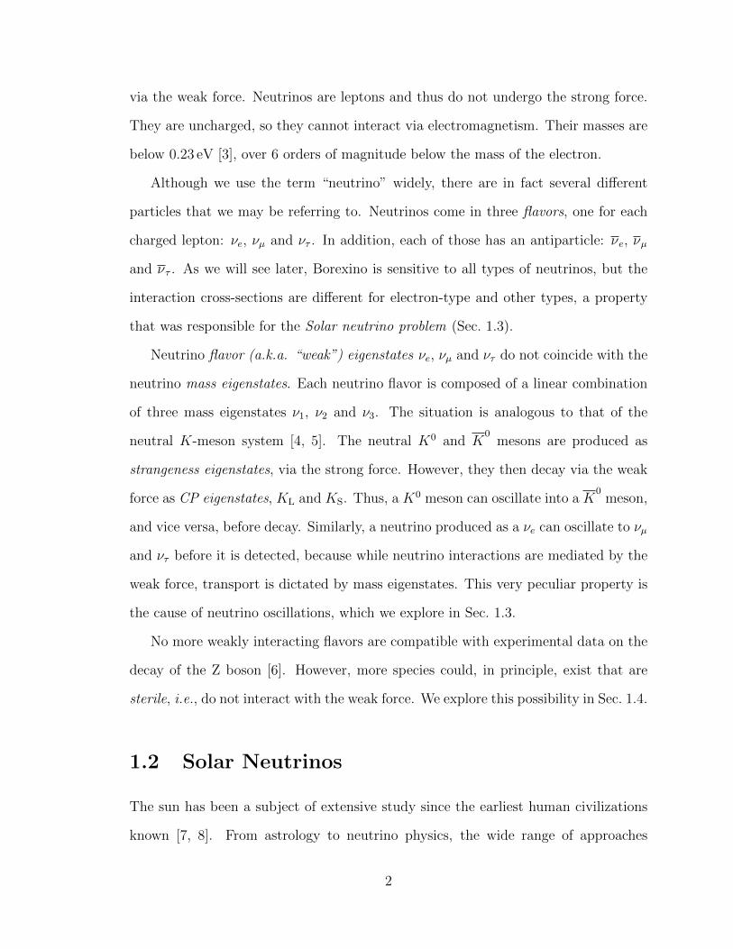
Neutrinos are chargeless, near-massless elementary particles. They were first proposed

by Wolfgang Pauli in 1930 as a way to resolve problems with the theory of β decay,

most notably conservation of energy. 1 Neutrinos were finally detected in 1956 [2]

through the reaction

νe + p+ → n0 + e+ (1.1)

Antineutrinos from a nuclear reactor triggered the reaction; neutrons were detected

through their capture γ rays (Borexino also detects neutrons in this manner, as we

will see in Chapter 6) and positrons were detected via annihilation with electrons.

Since then, neutrinos have been the subject of extensive theoretical and experimental

study. In this section, we outline some of the important properties of the neutrino,

and how they connect to the study presented in this thesis.

The challenge in studying neutrinos is intimately connected with the reason why

they are of interest in the field of solar astrophysics (Sec. 1.2): they can only interact

1The particle proposed by Pauli was actually called neutron, and it was thought to be a con-stituent of the nucleus, not created at emission time. It was renamed neutrino by Enrico Fermi afterChadwick’s discovery of what we now call the neutron in 1932. For more historical context, see [1].

1

via the weak force. Neutrinos are leptons and thus do not undergo the strong force.

They are uncharged, so they cannot interact via electromagnetism. Their masses are

below 0.23 eV [3], over 6 orders of magnitude below the mass of the electron.

Although we use the term “neutrino” widely, there are in fact several different

particles that we may be referring to. Neutrinos come in three flavors, one for each

charged lepton: νe, νµ and ντ . In addition, each of those has an antiparticle: νe, νµ

and ντ . As we will see later, Borexino is sensitive to all types of neutrinos, but the

interaction cross-sections are different for electron-type and other types, a property

that was responsible for the Solar neutrino problem (Sec. 1.3).

Neutrino flavor (a.k.a. “weak”) eigenstates νe, νµ and ντ do not coincide with the

neutrino mass eigenstates. Each neutrino flavor is composed of a linear combination

of three mass eigenstates ν1, ν2 and ν3. The situation is analogous to that of the

neutral K-meson system [4, 5]. The neutral K0 and K0

mesons are produced as

strangeness eigenstates, via the strong force. However, they then decay via the weak

force as CP eigenstates, KL and KS. Thus, a K0 meson can oscillate into a K0

meson,

and vice versa, before decay. Similarly, a neutrino produced as a νe can oscillate to νµ

and ντ before it is detected, because while neutrino interactions are mediated by the

weak force, transport is dictated by mass eigenstates. This very peculiar property is

the cause of neutrino oscillations, which we explore in Sec. 1.3.

No more weakly interacting flavors are compatible with experimental data on the

decay of the Z boson [6]. However, more species could, in principle, exist that are

sterile, i.e., do not interact with the weak force. We explore this possibility in Sec. 1.4.

1.2 Solar Neutrinos

The sun has been a subject of extensive study since the earliest human civilizations

known [7, 8]. From astrology to neutrino physics, the wide range of approaches

2

employed in its study is only a reflection of the amount of interest this object inspires

in us. We now know that the Sun is fueled by nuclear reactions [9]. In particular,

the “effective reaction” that takes place is the conversion of hydrogen (H) into helium

(He), with a net release of energy in the form of photons and neutrinos.

This conversion is complex, consisting of several steps, and its study is of great

interest to the understanding of star formation and evolution [10, 11]. This is due

to the fact that, while photons take about ten million years [2] to exit the sun,

neutrinos do so in a matter of seconds. Since the energy and flux of neutrinos produced

depends on the details of the hydrogen-burning reactions that take place in stars,

solar neutrinos are a probe of those details in the core of the sun, and that can be

extrapolated to other stars of its kind.

There are two main ways of converting protons (H) to α particles (He nuclei) that

take place in stars: the pp chain and the CNO cycle [11]. The contribution from each

of these processes depends on the size, temperature and age of the star [9]. In the

next sections we describe these sequences in detail, which will help us understand the

relevance of the pp neutrino analysis presented in this thesis.

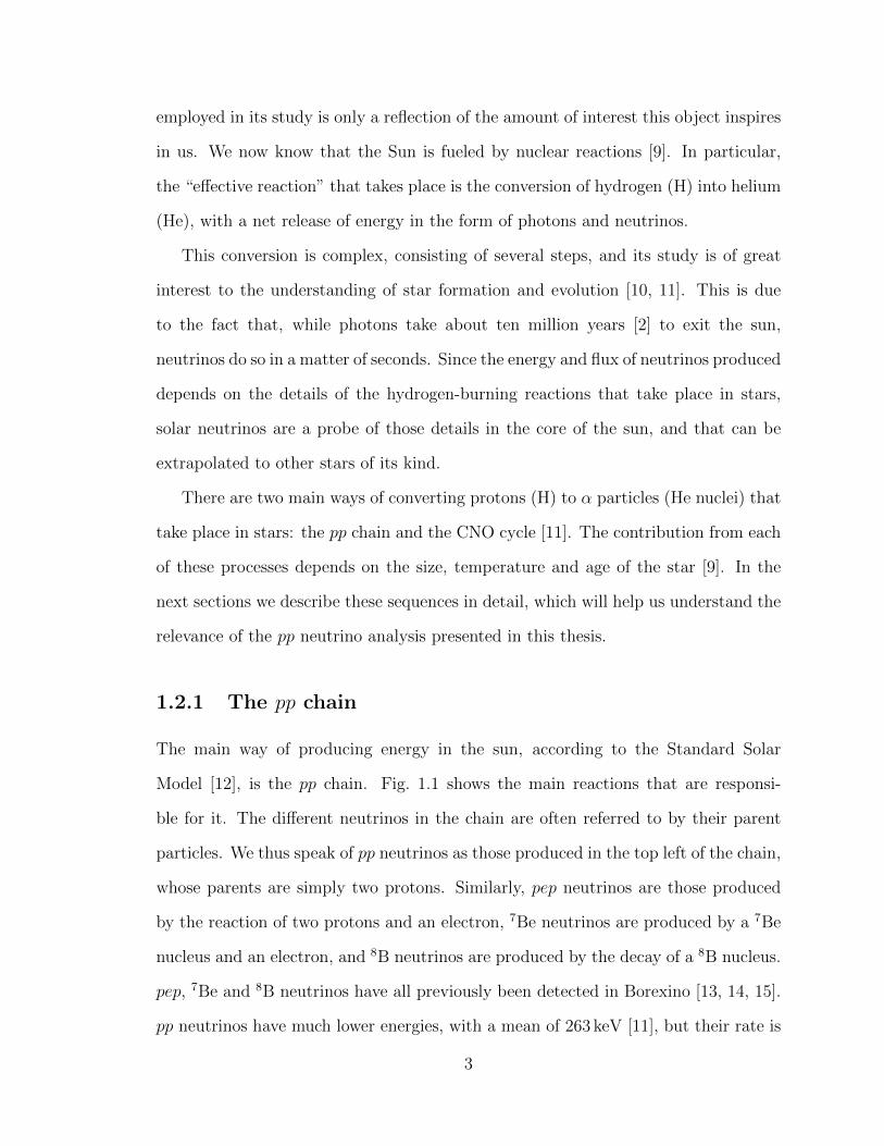
1.2.1 The pp chain

The main way of producing energy in the sun, according to the Standard Solar

Model [12], is the pp chain. Fig. 1.1 shows the main reactions that are responsi-

ble for it. The different neutrinos in the chain are often referred to by their parent

particles. We thus speak of pp neutrinos as those produced in the top left of the chain,

whose parents are simply two protons. Similarly, pep neutrinos are those produced

by the reaction of two protons and an electron, 7Be neutrinos are produced by a 7Be

nucleus and an electron, and 8B neutrinos are produced by the decay of a 8B nucleus.

pep, 7Be and 8B neutrinos have all previously been detected in Borexino [13, 14, 15].

pp neutrinos have much lower energies, with a mean of 263 keV [11], but their rate is

3

p + p d + e+ + ν p + e- + p d + ν

d + p 3He + γ

3He + 3He α + 2p 3He + α 7Be + γ

7Be + p 8B + γ8B 8Be + e+ + ν8Be 2α

7Be + e- 7Li + ν7Li + p 2α

Figure 1.1: Main nuclear reactions that make up the pp chain [11]. The neutrinosproduced by the chain are highlighted in magenta. Neutrinos are named after theparent particles that produce them (pp, pep, 7Be, 8B). pep, 7Be, and 8B neutrinos haveall been previously measured with Borexino [13, 14, 15], leaving only the pp neutrinos(top left) and the extremely faint hep neutrinos [10] (not shown here) undetectedprior to this work.

4

much higher than that of other neutrinos. This is the main feature that we exploit

in the present analysis.

1.2.2 The CNO cycle

Though most of the energy and neutrino flux in the Sun comes from the pp chain,

more massive and hotter stars produce much more significant amounts of energy

through the CNO cycle. In addition, a small component of the Sun’s neutrino flux

also comes from it.

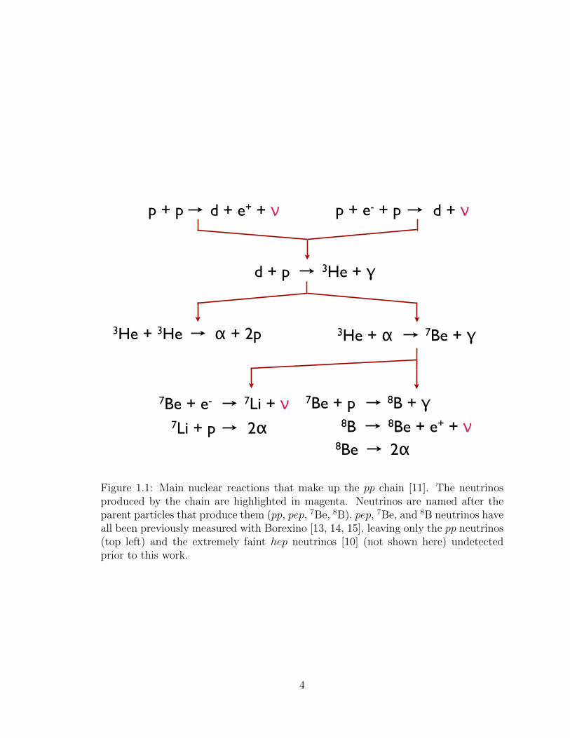
As opposed to the pp chain, the CNO cycle is thus named because carbon (C),

nitrogen (N) and oxygen (O) nuclei act simply as catalysts, their abundances not

modified by the hydrogen-burning process. Fig. 1.2 shows the main reactions that

make up the CNO cycle. Although the Sun mostly operates through the pp chain,

the CNO cycle is expected to contribute some fraction of the energy production.

However, CNO neutrinos have not been measured thus far, and only an upper limit

on their flux from the Sun has been placed by Borexino [13]. Work is underway to

improve this measurement and obtain the experimental rate.

The CNO cycle is of interest because it is responsible for most of the energy

production in stars bigger and hotter than the Sun [9, 16], and an understanding of it

can lead to improved stellar evolution models. For the present study, we assume the

CNO spectral rate and shape predicted by the Standard Solar Model [12]; we address

this further in Sec. 4.5.3.

1.2.3 Solar neutrino fluxes

The full energy spectrum of solar neutrinos as predicted by the Standard Solar

Model [12] is shown in Fig. 1.3. It includes all the neutrinos emitted by the pp

chain (Sec. 1.2.1) and CNO cycle (Sec. 1.2.2).

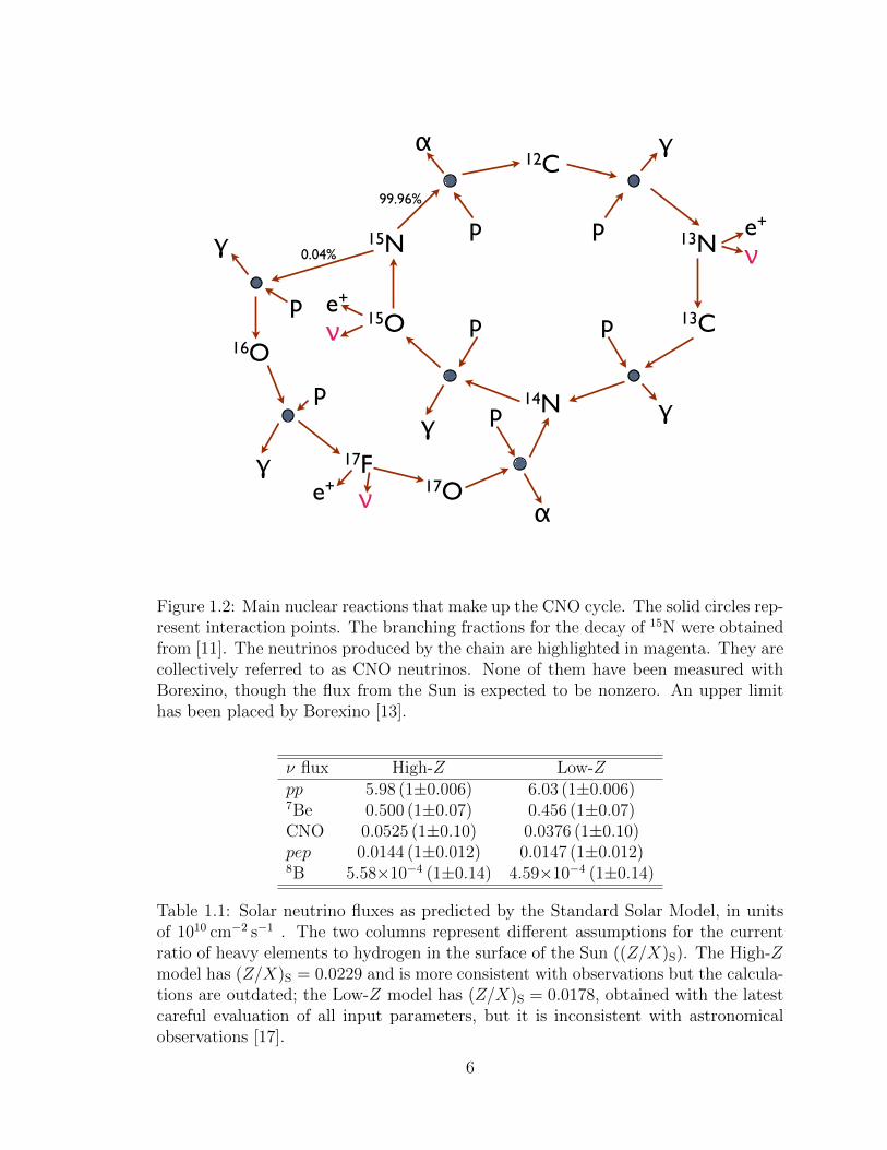
Tab. 1.1 lists the theoretical predictions for the solar neutrino fluxes [17]. The

5

12C

15O

15N

13C

13N

14N

p

γ

e+ν

p

γ

p

γ

e+ν

p

α

16O

17F17O

p

γ

p

γνe+

p

α

0.04%

99.96%

Figure 1.2: Main nuclear reactions that make up the CNO cycle. The solid circles rep-resent interaction points. The branching fractions for the decay of 15N were obtainedfrom [11]. The neutrinos produced by the chain are highlighted in magenta. They arecollectively referred to as CNO neutrinos. None of them have been measured withBorexino, though the flux from the Sun is expected to be nonzero. An upper limithas been placed by Borexino [13].

ν flux High-Z Low-Zpp 5.98 (1±0.006) 6.03 (1±0.006)7Be 0.500 (1±0.07) 0.456 (1±0.07)CNO 0.0525 (1±0.10) 0.0376 (1±0.10)pep 0.0144 (1±0.012) 0.0147 (1±0.012)8B 5.58×10−4 (1±0.14) 4.59×10−4 (1±0.14)

Table 1.1: Solar neutrino fluxes as predicted by the Standard Solar Model, in unitsof 1010 cm−2 s−1 . The two columns represent different assumptions for the currentratio of heavy elements to hydrogen in the surface of the Sun ((Z/X)S). The High-Zmodel has (Z/X)S = 0.0229 and is more consistent with observations but the calcula-tions are outdated; the Low-Z model has (Z/X)S = 0.0178, obtained with the latestcareful evaluation of all input parameters, but it is inconsistent with astronomicalobservations [17].

6

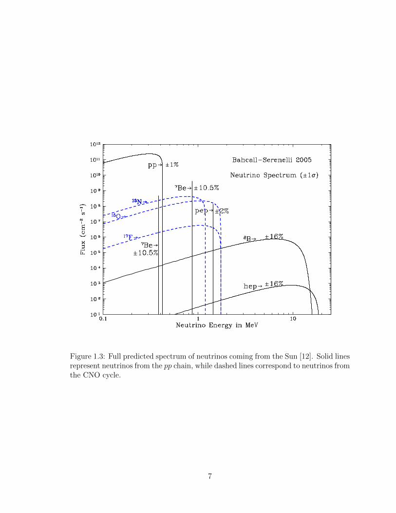
Figure 1.3: Full predicted spectrum of neutrinos coming from the Sun [12]. Solid linesrepresent neutrinos from the pp chain, while dashed lines correspond to neutrinos fromthe CNO cycle.

7

fact that there are two columns in the table is, in short, what is known as the “solar

abundance problem” or the “solar metallicity problem”. The two columns represent

two independent calculations of the fluxes. While the first column, labeled “High-

Z”, is more consistent with astronomical observations, the second column, labeled

“Low-Z”, is the one obtained using the most up-to-date evaluations of the nuclear

processes inside the Sun. The origin of the term “solar metallicity problem” is due

to the fact that astronomers name as “metals” any elements that are heavier than

hydrogen and helium. The two models presented here have different assumptions for

the ratio of “metals” to hydrogen in the present day in the surface of the Sun.

The values presented in Tab. 1.1 are the total fluxes of neutrinos arriving at Earth.

Neutrinos in the Sun are all produced as electron-type, νe. However, due to the MSW

effect [10], they change flavor due to their propagation inside the sun, and arrive at

Earth as a mixture of all three types: electron (νe), muon (νµ) and tau (ντ ). In the

energy range of pp neutrinos, the ν − e interaction cross-section is greater for νe as

compared to νµ,τ by a factor of about 3.5 [18]. Borexino is hence more sensitive to νe

than νµ,τ , and a measurement of the solar neutrino flux is a probe of the parameters

of the MSW effect. More details will be given in Sec. 1.3.

In addition, the predicted fluxes for some of the species are significantly different

between the High-Z and Low-Z models. A precision measurement of those species can

help validate one of these two models. The measurement of the 7Be neutrino rate in

Borexino, assuming the current best estimates for the parameters of the MSW effect,

resulted in a total neutrino flux of (4.84±0.24)×109 cm−2s−1 [14]. Unfortunately, this

lay right between the two models, and for that reason Borexino is now aiming to

measure the CNO neutrino flux, of which there is currently only an upper limit [13].

8

W− Z

νe,µ,τ e−, µ−, τ− νe,µ,τνe,µ,τ

Figure 1.4: Under the Standard Model, neutrinos can interact only under these in-teractions, plus their time-reversed versions.

1.3 Neutrino oscillations

In the Standard Model of particle physics (SM), neutrinos are massless fermions [19],

and their interactions are limited to three-body point-like interactions with the weak

bosons W and Z, as shown in Fig. 1.4. Fermions acquire mass through the Higgs

Mechanism. Neutrinos could be incorporated into the mechanism as well, with their

mass of the same order as that of the electron. We know from experiment, however,

that neutrinos are at least five orders of magnitude lighter than electrons [20]. The

most natural resolution of this apparent problem is to have neutrinos have no mass. In

addition, the Higgs mechanism gives mass to both left- and right-handed particles, and

right-handed neutrinos have never been measured. If neutrinos have no mass, their

flavor and mass eigenstates coincide, and there can be no transformations between

neutrinos of different generations.

Despite this theoretical prediction, the 37Cl experiment of Ray Davis and collab-

orators observed an apparent lack in the detection rate of neutrino electrons that

could naturally be explained by oscillations between different neutrino flavor eigen-

states [21]. Neutrino oscillations can only take place if neutrinos have mass, which is

9

in conflict with the SM. For this reason, physicists have become interested in measur-

ing neutrino oscillations, which might help us understand the extensions to the SM

that are required for neutrinos to have a mass.

The apparent neutrino detection rate deficit at the 37Cl neutrino experiment was

widely known as the “solar neutrino problem”. A proposed solution, known as the

“MSW effect”, states that neutrino oscillations can be significant even when the

mixing is rather small. The effect is due to the interaction of neutrinos with matter

inside the Sun [22].

Results from various experiments have since provided results consistent with the

MSW effect, which is currently the accepted explanation of the solar neutrino prob-

lem [23, 24].

Precision measurements of the neutrino oscillation parameters can shed light on

the mechanisms by which the oscillations take place and neutrinos acquire mass.

Borexino has the potential to perform some of these measurements, although the pp

neutrino interaction rate will not be significantly altered by variations in the theory.

A further analysis of CNO neutrinos, however, will provide a test of the different sets

of parameters allowed by the solar neutrino problem.

1.4 Sterile Neutrinos

Although the Standard Model (SM) and most of its popular extensions contain only

three species of neutrinos, the possibility of more species is not ruled out. Both the

number of relativistic species [3] and the number of active species [25] are constrained

to values close to 3, yet there is still the possiblity of non-relativistic sterile species.

Special interest has arisen after the discovery of a number of anomalies in the mea-

surements of neutrino oscillations [26, 27]. More recently, there have been a number

of analyses and re-analyses that have confirmed or refuted the existence of a “reactor

10

anti-neutrino anomaly” [28, 29]. The matter is not settled, however, and a possibility

for the existence of a fourth neutrino flavor still stands.

Borexino has the potential to be sensitive to a fourth species of neutrinos, with the

insertion of high-intensity radioactive sources of neutrinos and anti-neutrinos. The

collaboration has proposed to build the SOX experiment, which would make that

measurement within the next few years [30].

11

Chapter 2

The Borexino Detector

Borexino [31] is a liquid scintillator detector located at the Laboratori Nazionali del

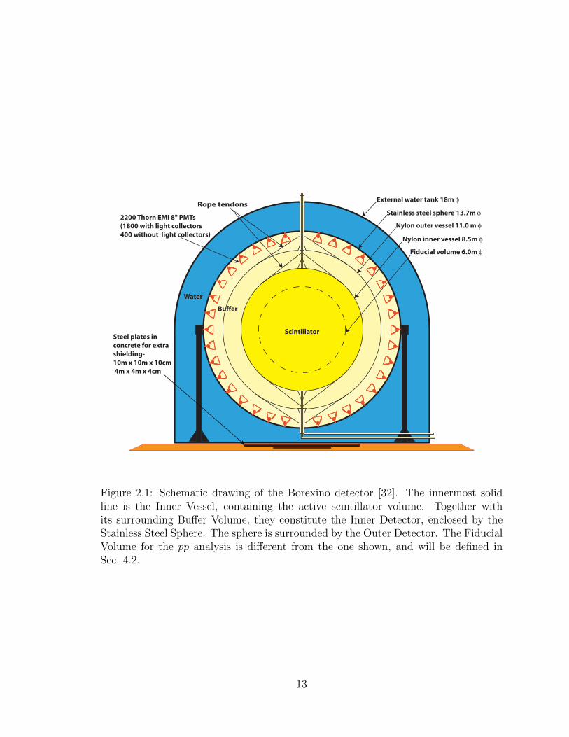
Gran Sasso (LNGS), an underground facility near L’Aquila, Abruzzo, Italy. A layout

of the detector is shown in Fig. 2.1. The Inner Detector (ID) consists of a Stainless

Steel Sphere (SSS; 13.7 m diameter) filled with the liquid scintillator pseudocumene

(PC). The Outer Detector (OD), surrounding the ID, is a domed cylindrical steel tank

filled with pure water, known as the Water Tank (WT; 17 m maximum height, 18 m

diameter), which acts as a Cherenkov detector. Inside the SSS, a spherical nylon Inner

Vessel (IV; 8.5 m diameter) divides the ID into two volumes: the active volume and

the Buffer Volume (BV). A second spherical nylon Outer Vessel (OV; 11 m diameter)

further divides the BV into two volumes. The principle of scintillation, the way it

can be used to detect neutrinos, and the purpose of the BV are explained in Sec. 2.1.

Light produced in the ID and OD is collected by photomultiplier tubes (PMTs) placed

on the walls of the Stainless Steel Sphere and on the floor of the Water Tank. The

detector hardware is described further in Sec. 2.2.

Borexino acquires data by triggering after scintillation events take place; this is

explained in Sec. 2.3. The energy and position of a scintillation event is determined

based on the distribution of photons detected by the PMTs. Sec. 2.4 describes the

12

Stainless steel sphere 13.7m φ

External water tank 18m φ

Nylon inner vessel 8.5m φ

Nylon outer vessel 11.0 m φ

Fiducial volume 6.0m φ

2200 Thorn EMI 8" PMTs(1800 with light collectors400 without light collectors)

Scintillator

Buffer

Water

Rope tendons

Steel plates in concrete for extrashielding-10m x 10m x 10cm 4m x 4m x 4cm

Figure 2.1: Schematic drawing of the Borexino detector [32]. The innermost solidline is the Inner Vessel, containing the active scintillator volume. Together withits surrounding Buffer Volume, they constitute the Inner Detector, enclosed by theStainless Steel Sphere. The sphere is surrounded by the Outer Detector. The FiducialVolume for the pp analysis is different from the one shown, and will be defined inSec. 4.2.

13

various energy estimators we use; our energy resolution is addressed in Sec. 2.5; in

Sec. 2.6 we go over the validation of the position reconstruction algorithm for the

present study.

At the location of Borexino in Hall C of the LNGS, the rock overburden is

∼3800 m water-equivalent. This is crucial for the elimination of cosmogenic back-

grounds. A review of the residual cosmogenic and radiogenic backgrounds, and of the

neutrino signals expected, is presented in Sec. 2.7. Finally, in Sec. 2.8, we describe

spectral-fitter, the tool we use for extracting the rates of signals and backgrounds

from our data.

2.1 Operating principle

The Borexino detector belongs to a beautiful class of experiments in which the target

material and the detection mechanism are essentially the same. Neutrinos impinging

on the detector scatter on electrons and nuclei in the scintillator. The moving charged

particles excite molecules along their way, which then de-excite and produce photons.

The final step in the detection mechanism is to collect the photons produced by the

scintillation mechanism. We employ photomultiplier tubes (PMTs), which convert

photons into electrons by the photoelectric effect, and then multiply those electrons

by secondary emission.

The number of photons produced by a scintillation event is related to the kinetic

energy of the moving charged particle that caused the scintillation by [33]

Nph = Yscint × E ×Q(E), (2.1)

where Yscint is the Light Yield of the scintillator, equal to approximately 438 pho-

toelectrons per MeV, E is the energy of the moving charged particle, and Q(E) is

the quenching factor at energy E. Yscint is measured in photons produced per unit

14

energy, and it is an intrinsic property of the scintillator. Quenching is a reduction of

the light production caused by the degradation of de-excitation processes [34]. The

quenching function is [35]

Q(E) =1

E

∫ E

0

dE′

1 + kB dEdx

(E ′)(2.2)

The stopping power dE/dx is a function of the energy of the moving particle, and

of the identities of the moving particle and the scintillator. kB is known as Birks’

constant, and it is an intrinsic property of the scintillator. However, for electron

recoils and β decays, we do not use the analytical equation, and instead employ an

empirical parametrization [36] similar to the one defined in [35]:

Qβ(E; kB) =A1 + A2 ln(E) + A3 ln2(E)

1 + A4 ln(E) + A5 ln2(E)(2.3)

where the parameters A1, A2, A3, A4, A5 are determined uniquely for each possible

kB [36] 1.

We note the unfortunate fact that the term “light yield” is often used to refer to

two quantities. One of them, which we also know as “scintillation yield” or Yscint is an

intrinsic property of the scintillator. The other, which we know as Ydet, is a property

of the detector and is measured in photoelectrons detected per unit energy. We talk

more about the latter in Sec. 2.5.

Since any moving charged particle will produce light by scintillation, a significant

source of background is due to radiogenic α, β and γ 2 particles. Borexino reduces

its background significantly by having a Buffer Volume (BV) outside of the detection

volume. In the BV, the PC is loaded with 5 g/l of dimethylphthalate (DMP), a

1For every value of kB, we first obtain a numerical approximation of Q(E) using Eq. 2.2 asimplemented in the program kB [37]. The resulting function is fit to Eq. 2.3 to extract the values ofA1, A2, A3, A4, A5.

2γs produce light by first scattering off electrons in the scintillator

15

scintillation quencher. A particle moving through the BV produces a much smaller

amount of scintillation light as compared to a particle moving through the Inner

Vessel (IV). Radiogenic particles from the external detector components will deposit

most of their energies in the buffer volume, with negligible light production. Note

that scintillation photons produced inside the inner detection volume will still travel

through the inactive liquid, which has the same index of refraction as the active

scintillator.

Radiogenic particles coming from contaminants in the liquid scintillator itself are

irreducible sources of background, i.e., they cannot be separated event-by-event. The

Borexino collaboration went through great trouble to mitigate the sources of radioac-

tivity inside the liquid, reaching unprecedented levels of radiopurity [38]. The Count-

ing Test Facility (CTF) was a prototype for the Borexino detector that demonstrated

that the liquid met the required levels of radioactivity [39]. Nevertheless, residual ra-

dioactive isotopes in the scintillator and in the external detector components continue

to be the limiting background in Borexino (see Sec. 2.7).

The presence of the stopping power dE/dx in Eq. 2.2 implies that different parti-

cles are quenched differently by the scintillator. In addition, when a moving particle

causes scintillation, the times at which photons are emitted relative to the initiation

of the motion of the particle follow a distribution dependent on the specific nuclear

processes taking place. These processes are different for different types of moving par-

ticles; in particular, α-decays tend to produce light for a longer time than β-decays

and electron recoils [36]. This fact is often employed in Borexino as a way to discrim-

inate backgrounds. More information on how this was used for previous analyses can

be found in [36].

Further details on the operating principle of Borexino can be found in [31].

16

2.2 Hardware

Fig. 2.1 shows a cross-section of the Borexino detector. The Inner Detector (ID) is

split in three sub-volumes by two concentric nylon spheres: the Inner Vessel (IV) and

the Outer Vessel (OV). As explained in Sec. 2.1, the spherical shell between the IV

and the SSS is known as the Buffer Volume (BV). The pseudocumene (PC) in the

BV is rendered inactive by addition of 5 g/l of DMP, a scintillation quencher. Radio-

genic particles coming from the external detector components deposit their energies

in the BV, which does not produce light, thereby reducing the background signifi-

cantly. Long-lived radioactive isotopes emanated by the SSS and the photomultipliers

(PMTs) can diffuse into the Buffer Volume. The OV serves to keep those particles

from decaying close to the active volume enclosed by the IV.

The liquid in the BV has the same index of refraction as the liquid in the IV;

thus, though the BV is inactive, it is transparent to light produced in the IV. This

makes the IV the active detector in Borexino. Inside the IV, the scintillator is loaded

with 1.5 g/l of the wavelength shifter 2,5-diphenyloxazole (PPO). The shift in wave-

length improves the time response and matches better the photomultiplier quantum

efficiency window [31].

The ID is contained within the 13.7-m-diameter Stainless Steel Sphere (SSS). The

inside of the sphere is equipped with 2212 8” ETL-9351 photomultiplier tubes [31] to

detect the light coming from within the Inner Vessel (IV), the central 8.5-m-diameter

sphere. The scintillation efficiency Yscint of the liquid scintillator (PC + PPO) inside

the IV is (11500±10%) photons/MeV [40]. After accounting for solid angle covered

by PMTs, reflectivity of the internal SSS wall surfaces and detection efficiency of the

PMTs, the expected light collection efficiency Ydet is ∼500 p.e./MeV [33], where p.e.

denotes photoelectrons. Further details about the second quantity are provided in

Sec. 2.5.

17

A PMT converts photons into electrons through the photoelectric effect. The

resulting electrons, also known as photoelectrons, are then multiplied by secondary

emission, resulting in a charge measurement at the PMT output. The mapping

between the charge collected at the PMT output and the number of photoelectrons

produced by the photoelectric effect is calibrated with light pulses [31]. Most of the

PMTs in Borexino are equipped with light concentrators to increase light collection

efficiency [33].

The nylon vessels and the end caps at the top and bottom of them have intrinsic

radioactivity that can produce scintillation in the IV. Moreover, residual radioactive

isotopes from the SSS, the PMTs and the light concentrators diffusing through the

OV and into the inner buffer volume can also decay close to the IV. We deal with

this by applying a Fiducial Volume cut (see Sec. 4.2). To apply such a cut, we must

be able to reconstruct the positions of scintillation events; see Sec. 2.6. More details

on the ID can be found in [31].

A leak was discovered in one of the nylon vessels in 2008. Though this was a

major turning point for Borexino, the engineers were able to tune the flow of different

liquids into and out of the detector in a way that minimizes the motion of liquid

across the interface formed by the hole in the vessel. A full report on the leak is

provided in [36].

The Outer Detector (OD) acts as both active and passive shielding from external

radiogenic and cosmogenic particles that act as backgrounds to the neutrino sig-

nals. The active shielding comes from the detection of Cherenkov light by 208 PMTs

mounted on the outer wall of the SSS and on the floor of the external water tank.

Details of the OD hardware and electronics are given in [41]. For the pp analysis, the

OD was used for tagging muons with an efficiency greater than (99.33±0.01)%.

18

2.3 Data Acquisition

We present a brief outline of the electronics and triggering of Borexino, which are used

to interpret photons collected by the PMTs as scintillation events in the detector. We

focus on the parts that are most relevant to the pp analysis; a more detailed description

was presented in [36].

Borexino PMTs are connected to two electronic circuits: one of them serves for

triggering; the other one, for measuring the number of photons arriving at the PMT.

A “triggered” PMT is one that has detected at least one photon; more precisely, we

consider a PMT to have triggered if the charge registered by the PMT exceeds ∼1/5

of the mean charge corresponding to a single photoelectron [31].

When more than a number K of phototubes “fire” (i.e. trigger) within 60 ns [33],

a detector event is triggered. The waveform on all triggering photomultipliers is then

sampled and digitized by a 8-bit flash ADC for 16µs after the event trigger. Offline,

i.e., after data is acquired, a piece of software named Echidna looks for hits, i.e.,

triggering photomultipliers, in the waveforms. A typical Borexino raw trigger event

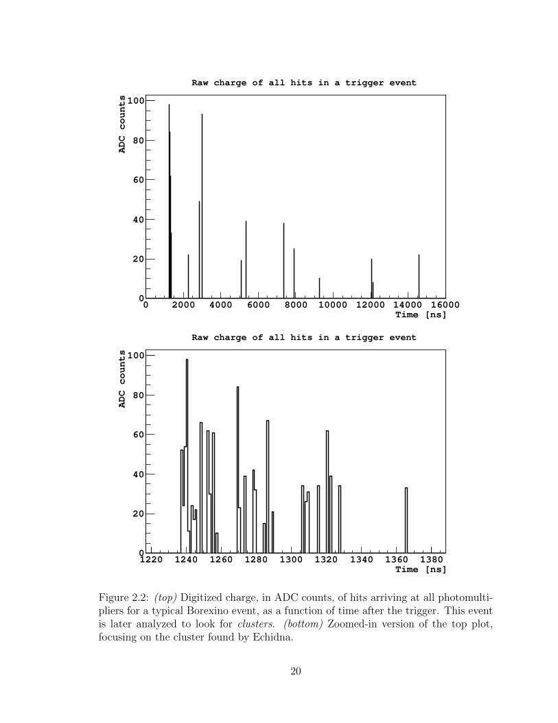
after hit reconstruction is shown at the top of Fig. 2.2. A certain dark rate is expected

due to intrinsic noise in the photomultipliers, and it is on the order of 15 hits per

16-µs time window. The trigger threshold K was previously set to 25 hits, and was

changed to 20 hits around March 2013, to collect data at lower energies. The trigger

efficiency is, however, a continuous function of the number of hits, and near-perfect

trigger efficiency only kicks in around 40-50 hits.

There are different types of triggers, for different physical events, as shown on

Tab. 2.1. For all types of triggers, data is collected from all the Inner Detector and

Outer Detector PMTs. The piece of hardware responsible for raising trigger con-

ditions is known as the Borexino Trigger Board (BTB) [43]. The different inputs

arriving at the BTB generate different trigger types. Trigger type 1 is the one de-

scribed above, and it is the expected trigger type for regular neutrino interaction

19

Time [ns]0 2000 4000 6000 8000 10000 12000 14000 16000

ADC counts

0

20

40

60

80

100

Raw charge of all hits in a trigger event

Time [ns]1220 1240 1260 1280 1300 1320 1340 1360 1380

ADC counts

0

20

40

60

80

100

Raw charge of all hits in a trigger event

Figure 2.2: (top) Digitized charge, in ADC counts, of hits arriving at all photomulti-pliers for a typical Borexino event, as a function of time after the trigger. This eventis later analyzed to look for clusters. (bottom) Zoomed-in version of the top plot,focusing on the cluster found by Echidna.

20

N0 Name BTB input Priority1 Neutrino 0 12 MTB 4 24 Laser 355 16 48 Laser 394 64 716 Laser 266 32 532 Pulser 64 664 Random 64 8128 Neutron 8 3

Table 2.1: Trigger types available in Borexino. The pp analysis is done only onevents of trigger type 1, which is generated when the number of photomultipliers hitin a 60-ns time window exceeds the BTB threshold. Trigger type 64 events wereused for dark noise convolution. The laser and pulser types are used for PMT andelectronics calibrations. MTB triggers are mostly muons crossing the outer detector,and neutron triggers are 1.6-ms DAQ windows opened after muons cross the innerdetector. Whenever a trigger of any type is generated, we record the sum of the BTBinputs bit field. Thus, if a type 1 trigger is generated while the random trigger inputwas on (BTB input 64), the trigger type will be 1, but the BTB inputs flag will be64. The priority is in place to resolve conflicts. [42]

events. Laser and pulser triggers are induced every ∼2 s by lasers pointing at the

PMTs and by electrical pulses, respectively, and they are used for calibration and

monitoring (e.g., to map the charge collected at the PMT outputs and the number

of photoelectrons created by the photoelectric effect, as we saw in Sec. 2.2). Trigger

types 4, 8 and 16 are laser triggers with different laser wavelengths; trigger type 32

are pulser triggers. Trigger type 64 are regularly solicited trigger events, acquired at

0.5 Hz, in which data is collected for 16µs regardless of the number of PMT hits reg-

istered in that time window. These solicited events, also known as “random triggers”,

are used for monitoring the dark rate in the detector, and for background estimates

(Sec. 4.3.1). The OD also has a hardware piece dedicated to triggering, known as

the Muon Trigger Board (MTB). It raises the Muon Trigger Flag (MTF) whenever

more than 6 OD PMTs fire within 150 ns [41]; this is trigger type 2. Trigger type

128 occurs when both the OD and the ID trigger within a small time window of each

other, in which case a 1.6-ms time window is opened for recording neutrons, which

21

have capture times of ∼250µs [44]. The overall Borexino trigger rate for K ∈ (20, 25)

is in the range 20-35 Hz.

Note from Tab. 2.1 that there is not a one-to-one correspondence between trigger

types and BTB inputs. This is for two reasons. The first one is that there are not

as many BTB inputs as there are trigger types, so that some BTB inputs generate

multiple types of triggers. The second reason is that, in some cases, triggers are

converted from one type to another online; for example, if a scintillation event is

detected at the beginning of a random trigger, it will be triggered by BTB input 64,

but it will become a trigger type 1 instead of a trigger type 64.

In each trigger, a clustering algorithm looks for groups of hits that represent

scintillation events, also known as clusters. We use two independent pieces of software

for clustering: Echidna (also responsible for finding the individual hits, as mentioned

above) and Mach4 3. Most triggers contain at most one cluster, but some multi-cluster

triggers are observed. A typical cluster in a Borexino event is shown at the bottom

of Fig. 2.2. After clusters are found, various energy estimators and timing variables

are calculated from the information contained in the hits. A position reconstruction

algorithm is also run to estimate the locations of the physics events.

The triggering process described above is entirely equivalent to that used for

previous analyses. Two modifications were made for the measurement of the pp

neutrino detection rate, namely,

• The decrease of the event trigger threshold K from 25 to 20

• The elimination of “hot” (i.e., very noisy) PMTs before the application of clus-

tering algorithms

3In the past, Echidna and Mach4 were completely independent software packages, each includingits own hit-, cluster-, energy- and position-reconstruction algorithms. In the present study, Mach4begins data processing after Echidna hit-reconstruction; this implementation is known as “Mach4Over Echidna” (MOE). We thus use both the terms “Mach4” and “MOE” interchangeably to referto MOE. For a complete report of the Mach4-Echidna history, see [33].

22

The second modification reduces the amount of light collected, but it also reduces the

proportion of dark noise, which could be significant at the low energies characteristic

of pp-neutrino-induced electron recoils. We come back to this point in Sec. 2.8.2. The

newest version of Echidna, after these modifications, is known as “Echidna Cycle 16”.

2.3.1 Neutron DAQ

Liquid scintillator is a promising tool for the reduction of neutron-induced background

in dark matter detectors [45]. Studies have been performed using Monte Carlo simula-

tions of liquid scintillator detectors to estimate the capabilities of cosmogenic neutron

detection [46]. Borexino has the capability to actually detect cosmogenic neutrons and

measure their capture times and travel distances. Cosmogenic neutrons are spawned

by spallation by cosmogenic muons, and they are captured in liquid scintillator within

∼250µs [41]. At the beginning of Borexino, it was noticed that whenever a muon

crossed the ID, it would saturate the boards, and no hits would be registered for

400µs thereafter.

While the main DAQ was being upgraded to eventually implement trigger type 128

in late 2007, another system was installed, called the Princeton Analog System (PAS),

also known as Analog DAQ. The system triggers every time the MTF condition is

raised (see Sec. 2.3). An Acquiris DP235 digitizer collects data for 1.6 ms thereafter.

An online coarse cut eliminates triggers that do not appear to contain any neutrons.

A secondary, more refined cut is implemented offline to select neutrons with high

efficiency.

The main advantage of this system is that it can detect neutrons with very high ef-

ficiency, without the saturation that still occurs in the main DAQ. The disadvantage

is that no position reconstruction can be attempted, for we do not have informa-

tion from individual PMTs. This system and its results will be discussed further in

Chapter 6.

23

2.4 Energy estimators

Both Echidna and MOE return a list of triggers with their corresponding clusters and,

for each cluster, a series of energy estimators. There are two pieces of information

arriving at PMTs that can be used to construct energy estimators: the hits arriving

at PMTs, and the charge collected by the PMTs in those hits.

To estimate the energy based on hits, we count the number of hits arriving at

PMTs within the length of the reconstructed cluster. If we count all the hits, including

multiple hits on single PMTs, we are referring to nhits. If, instead, we count only

the number of PMTs hit, regardless of how many times each PMT was hit, we are

computing the variable npmts.

The second possible way of estimating the energy of an event is by summing up

the charge recorded for every hit arriving within the cluster duration. We call that

variable npe.

The number of channels available for photon detection varies with time, as failures

of the electronics cause PMTs to be unavailable temporarily, and as some PMTs shut-

off permanently due to more serious failures. One way to account for this variation

is to normalize event-by-event the values of the energy estimators, by multiplying

them by a factor equal to 2000 divided by the number of working channels. Such

variables are said to be normalized or equalized, and we can write them as npmtsnorm,

nhitsnorm, and npenorm. In the present study, we account for the variation in the

number of available PMTs in a different way, explained in Sec. 2.5.

Note that nhits and npmts will include dark noise hits. We describe the procedure

through which we account for those in Sec. 2.8.2. As we will see, this procedure

requires that all clusters have a fixed pre-defined duration. This is in contrast to the

standard procedure, in which the clustering algorithm decides where the cluster ends

based on the distribution of hits or the beginning of a new cluster. Variables with a

fixed cluster duration will include all hits arriving within a certain time window after

24

Name Definitionnpmts Number of PMTs hit in a cluster, ignoring multiple hits on PMTsnhits Number of PMT hits in a cluster, including multiple hits on PMTsnpe Charge collected in all PMT hits in a clusternpmtsnorm npmts re-normalized to 2000 active PMTsnhitsnorm nhits re-normalized to 2000 active PMTsnpenorm npe re-normalized to 2000 active PMTsnpmts dt1 Number of PMTs hit within 230 ns after the cluster start timenpmts dt2 Number of PMTs hit within 400 ns after the cluster start timenpmts win1 Number of PMTs hit in each 230-ns window in random triggersnpmts win2 Number of PMTs hit in each 400-ns window in random triggers

Table 2.2: All the Borexino energy estimators defined in Sec. 2.4. All the estimatorsin the top section are computed for each cluster. The bottom two estimators arecomputed for each time window of the specified length obtained by splitting randomtriggers (trigger type 64).

cluster start, regardless of what happens during that time window. For the present

analysis, we have created two such variables, npmts dt1 and npmts dt2, which include

PMTs hit within 230 ns and 400 ns, respectively, after the beginning of each cluster.

If a second cluster begins before the end of the first cluster, some PMT hits will be

counted in the estimators for both clusters.

Another set of estimators was implemented for random triggers (trigger type 64,

see Tab. 2.1). To make an estimate of the amount of dark noise in the detector,

we divide random triggers into smaller windows of size ∆t, and count the number of

PMTs hit within each of those smaller windows. Two values of ∆t were implemented,

corresponding with the durations of npmts dt1 (230 ns) and npmts dt2 (400 ns). The

resulting variables are npmts win1 and npmts win2. Their distributions can be in-

terpreted as the probability distributions for npmts dt1 and npmts dt2 in random

noise.

The energy estimators defined in this section are summarized in Tab. 2.2. We

relate some of these estimators to the energy deposited by moving charged particles

in the next section. More details regarding the different variables available in the

Borexino analysis software can be found in [36].

25

2.5 Energy resolution

In the pp analysis, we represent our data by using the energy estimators npmts dt1

and npmts dt2, defined in Sec. 2.4. In the present section, we refer to all npmts-like

variables as Np, which denotes the number of PMTs hit, without specifying the time

window during which we count them. Neutrino- and muon-induced recoils, radioactive

decay of natural contaminants, and radioactive decay of cosmogenic isotopes all have

their own characteristic energy spectra; we review some of that information in Sec. 2.7.

To model our data, we have to convert all the expected energy spectra into the Np

variable.

For a given species j, let its energy spectrum be hj(E). We convert that distribu-

tion to a spectrum in the Np variable, Hj(Np), according to

Hj(Np) =∑E

f(Np|E) hj(E) (2.4)

where f(Np|E) is the energy response function or energy resolution function. It can

be interpreted as the probability distribution for Np given energy E. The sum goes

over all points at which the energy spectrum is available.

We assume that the response function is a Scaled Poisson function [47]:

f(Np|E) =µsNp

Γ(sNp + 1)e−µ (2.5)

26

where µ and s are two energy-dependent parameters that can be related to the mean 4

and variance of the distribution by the relations [47]

Np(E) =µ

s(2.6)

σ2Np(E) =

µ

s2

Γ is the gamma function, a generalization of the factorial to real numbers, which for

positive integers n is Γ(n) = (n − 1)!. For positive real numbers y, it is defined as

Γ(y) =∫∞

0ty−1e−t dt and is typically evaluated numerically. The assumption that

the response function follows Eq. 2.5 is based on a recent study [48] in which a

high-statistics sample of simulated 14C β decays was compared to analytical shapes

obtained with various choices for the response function. Previous analyses used a

Generalized Gamma function [49, 36], which was a good match for charge variables,

not npmts-like variables (Np).

We now evaluate Np(E), which is the mean value of the Np variable expected for

energy E, and σ2Np

(E), its variance. Those will then be connected to µ and s, the

parameters of the β response function, by Eq. 2.6.

Suppose a scintillation event of energy E takes place inside the Inner Vessel. The

number of photons produced by the scintillator is given by Eq. 2.1. After account-

ing for volume effects, quantum efficiency of the phototubes and other effects, the

corresponding number of detected photoelectrons, Npe, will be [36]:

Npe = Ydet · E ·Qp(E) (2.7)

4Note that Np is a variable, while ε(Np(E)) is the mean or expected value of the variable Np atenergy E. For a more concise notation, here we simplify ε(Np(E)) as Np(E). In what follows, wesometimes omit the explicit energy dependence, and we still intend that Np is an expected value.When necessary, we will re-insert the energy dependence for clarity.

27

where Ydet is the fiducial-volume-averaged detector light yield, and Qp(E) is the

quenching factor for particle type p 5, given by Eq. 2.2 6. Ydet will be different

for different Np variables: as light is collected during more time in npmts dt2 with

respect to npmts dt1, the value of Ydet will be higher for npmts dt2 as compared to

the value for npmts dt1. The number of photoelectrons collected, on average, by one

PMT, is

µ0 = Npe/Nlive (2.8)

where Nlive is the number of live PMTs at the time of the event (Nlive is varies

with time, as PMTs become inactive; see Sec. 2.4). The distribution of the detected

photoelectrons at each PMT is expected to be Poissonian [36]. Thus, the probability

of having a signal at any one PMT is

p1 = 1− e−µ0 (2.9)

The mean number of PMTs hit, Np, assuming the event takes place at the center of

the detector would be

N ctrp = Nlive · p1 = Nlive · (1− e−µ0) (2.10)

When we consider events taking place in the entire Fiducial Volume, Np becomes a

function of the position of the event. This is due mostly to solid angle corrections. A

5In the terminology of [36], we have set N0pe, which represents a systematic shift due to dark noise,

to 0. This is justified because, as we will see in Sec. 2.8.2, we include dark noise in our analyticalspectra by convolving them with a real sample of noise.

6Here we have explicitly inserted the dependence on particle type p given by the stopping power.

28

correction was found empirically [14, 36]:

µ0g ≡ Npe/(Npe · cg +Nlive) (2.11)

p1g ≡ 1− e−µ0g (2.12)

Np = Nlive · p1g (2.13)

where cg = 0.122 is a geometrical correction factor that accounts for the fact that

there are events taking place in the entire Fiducial Volume (FV), and as such is a

function of the choice of Fiducial Volume. cg is independent of the number of live

PMTs. Adding the explicit time dependence, we can write

Np(t) = Nlive(t) · p1g (2.14)

Although the definition of p1g contained a dependence on Nlive, and therefore on time,

p1g itself is time-independent 7: in Eq. 2.7, Ydet is proportional to Nlive(t)8 [36]. and

thus the time-dependence of µ0g in Eq. 2.11 cancels out. The final expression for the

time-averaged expectation value of the Np variable is

Np(E) ≡ Np(E, t) = Nlive(t) · p1g(E) (2.15)

where the energy dependence has been written explicitly, and the overline represents

averaging over time.

We must now calculate the variance σ2Np

. Let us first assume that we perform

the experiment at time t, so that the number of live PMTs is fixed at Nlive(t), and

that the events all take place at a fixed position ~r. 9 For an event of energy E, the

7Another way to say this is that the mean number of photoelectrons on a given PMT does notchange if another PMT dies.

8This is intuitive: if all PMTs behave roughly the same way, the more you have, the morephotoelectrons will be detected for a given energy.

9The assumption that β events are point-like is justified by their short range. Our energiesof interest will be ∼500 keV (Fig. 1.3). 500-keV βs have a range of about 0.01 cm [50], getting

29

probability that PMT i will be hit is pi1(E,~r), such that

ε(Np(E,~r, t)) =

Nlive(t)∑i=1

pi1(E,~r) (2.16)

is the expected (central) value of theNp variable, with the sum running over live PMTs

only. Assuming that we can treat PMTs independently, we can add their individual

variances, and so we can write, assuming each of them behaves binomially [36],

σ2Np(E,~r, t) =

Nlive(t)∑i=1

pi1(E,~r) ·[1− pi1(E,~r)

]= ε(Np(E,~r, t))−Nlive(t) ·

1

Nlive(t)

Nlive(t)∑i=1

[pi1(E,~r)

]2(2.17)

Noting that the last part is a mean of a variable squared, and using the identity

σ2q = 〈q2〉 − 〈q〉2,

σ2Np(E,~r, t) = ε(Np(E,~r, t))−Nlive(t) ·

(σ2

1(E,~r) + p21(E,~r)

)(2.18)

where the mean p1(E,~r) is defined from Eq. 2.16:

p1(E,~r) ≡ 1

Nlive(t)·Nlive(t)∑i=1

pi1(E,~r) =ε(Np(E,~r, t))

Nlive(t)(2.19)

Note that we are assuming that p1(E,~r), that is, the mean probability for any given

PMT to detect at least one photoelectron, and its variance σ21(E,~r), are independent

of time. This is roughly equivalent to assuming that the position distribution of

PMTs is constant in time, so that no configuration of PMTs favors less or more

variability in the probability for each PMT of detecting a photoelectron. We checked

this assumption by looking at the position distributions of PMTs in five randomly

even smaller at lower energies, while the uncertainty in the Borexino position reconstruction is∼1-10 cm [36].

30

selected runs roughly evenly distributed throughout the data acquisition period. The

distributions were consistent with each other. Now we can define the relative variance

v1(E,~r) = σ21(E,~r)/p2

1(E,~r) to obtain

σ2Np(E,~r, t) = ε(Np(E,~r, t))−Nlive(t) · p2

1(E,~r) · (1 + v1(E,~r)) (2.20)

Using Eq. 2.19 once again,

σ2Np(E,~r, t) = ε(Np(E,~r, t)) · [1− p1(E,~r) · (1 + v1(E,~r))] (2.21)

This would be the variance in an experiment where all events occurred at fixed

position ~r and time t. To account for the variations in those parameters, we must

calculate the grand σ2Np

(E) variance:

σ2Np(E) =

⟨ε(N2

p (E,~r, t))⟩− 〈ε(Np(E,~r, t))〉

2(2.22)

where, for any variable q, 〈q〉 is the average of q over the entire Fiducial Volume and

q is the average of q over time. Applying the variance identity once again:

σ2Np(E) =

⟨σ2Np

(E,~r, t) + ε2(Np(E,~r, t))⟩− 〈ε(Np(E,~r, t))〉

2(2.23)

where σ2Np

(E,~r, t) is the purely statistical variance of Eq. 2.21, so that

σ2Np(E) = 〈ε(Np(E,~r, t)) [1− p1(E,~r) (1 + v1(E,~r))]〉+〈ε2(Np(E,~r, t))〉−〈ε(Np(E,~r, t))〉

2

(2.24)

We introduce some new notation, to simplify the equations. First, we remove the

explicit dependence on E, and assume that all our derivations are for a fixed energy.

We re-insert the energy dependence at the end. Let us also simplify the nomenclature

31

for the expected value ε(Np(E,~r, t)) as simply Np(~r, t). Therefore,

σ2Np = 〈Np(~r, t) · (1− p1(~r) (1 + v1(~r)))〉+

⟨N2p (~r, t)

⟩− 〈Np(~r, t)〉

2(2.25)

At this point, it is useful to introduce the volumetric relative variance:

vT (〈Np(~r, t)〉) ≡⟨N2p (~r, t)

⟩− 〈Np(~r, t)〉2

〈Np(~r, t)〉2(2.26)

Using this definition, we can rewrite Eq. 2.25 as

σ2Np = 〈Np(~r, t) · (1− p1(~r) (1 + v1(~r)))〉+ (vT (〈Np(~r, t)〉) + 1) 〈Np(~r, t)〉2−〈Np(~r, t)〉

2

(2.27)

Next we make a few assumptions that will allow us to obtain a result in an easily

manageable way.

Assumption 1:

〈Np(~r, t) · (1− p1(~r) (1 + v1(~r)))〉 = 〈Np(~r, t)〉 · 〈1− p1(~r) (1 + v1(~r))〉 (2.28)

This can be interpreted as follows: since p1 is small, and the geometric effect is

also expected to be small, we can treat them both only to first order. With this

assumption, we can write

σ21Np

=〈Np(~r, t)〉 · [1− 〈p1(~r)〉 (1 + v1)]

+ (vT (〈Np(~r, t)〉) + 1) 〈Np(~r, t)〉2 − 〈Np(~r, t)〉2

(2.29)

32

where v1 ≡ 〈p1(~r)v1(~r)〉 / 〈p1(~r)〉. Using Eq. 2.19 with the new notation introduced

after Eq. 2.24, and with the new notation Np(t) ≡ 〈Np(~r, t)〉, we get

σ21Np

= Np(t) ·[1− Np(t)

Nlive(t)(1 + v1)

]+ [1 + vT (Np(t))] ·N2

p (t)−Np(t)2

(2.30)

Now note that Np(t) is the space-averaged time-dependent expectation value of the

Np variable as a function of time, as given in Eq. 2.14, so that, defining f(t) ≡

Nlive(t)/Nfixed,

σ21Np

= Nfixedf(t) p1g

[1− p1g (1 + v1)

]+ [1 + vT (Np(t))]

(Nfixedf(t) p1g

)2 −Np(t)2

(2.31)

Assumption 2:

vT (Np(t)) = vT (Np(t)) (2.32)

This is based on empirical observation from [36]. Implementing this assumption, plus

the notation Np = Np(t),

σ22Np

= Nfixed p1g

[1− p1g (1 + v1)

]f(t) + [1 + vT (Np)] (Nfixed p1g)

2 f 2(t)−N2p (2.33)

Once again, we define a relative variance vf =[f 2(t)− f(t)

2]/f(t)

2to write 10

σ22Np

= Nfixed p1g

[1− p1g (1 + v1)

]f(t) + [1 + vT (Np)](Nfixedp1g)

2f(t)2

(vf + 1)−N2p

= Np

[1−Np/Nlive (1 + v1)

]+ [vf + vT (Np) + vfvT (Np)]N

2p (2.34)

Assumption 3:

vT (Np) = v0T Np (2.35)

10 As can be seen in the top panel of Fig. 2.3, assuming that the distribution of Nused can bedescribed just by its mean and variance, like a Gaussian distribution, is not justified. The effect ofthis assumption on the final pp result was found to be negligible through studies performed by theworking group.

33

where v0T is a constant. This was based on a MC modeling done in [36]. Using this

assumption, we get our preliminary result:

σ23Np

= Np

[1−Np/Nlive (1 + v1)

]+ [vf + v0

TNp + vfv0TNp]N

2p (2.36)

One additional component needs to be included. Known as a “pedestal” term,

σ2ped, it accounts for the presence of a variance that does not arise from scintillation

events, and is therefore uncorrelated with the energy. This gives us our final result

σ2Np(E) = Np(E)

[1−Np(E)/Nlive (1 + v1)

]+(vf + v0

TNp(E) + vfv0TNp(E)

)N2p (E)+σ2

ped

(2.37)

where we have inserted the energy dependence explicitly.

We can now use Eqs. 2.15 and 2.37 to calculate µ and s as in Eq. 2.6; those

parameters are plugged into the energy response function of Eq. 2.5 to convert energy

spectra to Np as in Eq. 2.4. For convenience, we reproduce them here in consistent

notation:

Np(E) = Nlive

[1− exp

( −Ydet · E ·Qp(E; kB)

Ydet · E ·Qp(E; kB) · cg +Nlive

)]σ2Np(E) = Np(E)

[1− Np(E)

Nlive

(1 + v1)

]+[vf + v0

TNp(E) + vfv0TNp(E)

]N2p (E) + σ2

ped

µ =N2p (E)

σ2Np

(E); s =

Np(E)

σ2Np

(E)

Hj(Np) =∑E

µsNp

Γ(sNp + 1)e−µ hj(E) (2.38)

Note, once again, that Np(E) is the mean or expected value of the variable Np at

energy E, and N2p (E) = [Np(E)]2; note further that Np represents any variable that

is constructed by counting the number of PMTs hit, which in the present analysis

will typically be npmts dt1 or npmts dt2. Nlive and vf are determined from the

distribution shown at the top of Fig. 2.3. v1 = 0.16 was calculated by the pp working

34

usedN1600 1620 1640 1660 1680 1700 1720 1740 1760 1780

Eve

nts

0

50

100

150

200

250

300

310× Live minus invalid PMTs

Run number17500 18000 18500 19000 19500 20000 20500

live

N

0

200

400

600

800

1000

1200

1400

1600

1800

vs run numberliveN

Figure 2.3: (top, solid black line) Distribution of used (live minus invalid) PMTsin events with npmts dt1 close to the expected value for 14C (see Fig. 2.4) duringperiods 9 thru 11 combined. The mean number is 1705, considerably lower than thenominal value of 2000. The standard deviation is 42. (top, dashed red line) Samedistribution, weighted by approximate amount of 210Po remaining at the time of theevent. See Sec. 2.7.2.3 for details. (bottom) Scatter plot of number of live PMTsversus run number, for periods 9–11. 35

group 11. Ydet, v0T and σped are a priori unknown; we determine them by leaving them

free in our spectral fit (Sec. 2.8). The value of kB will be discussed in Sec. 4.3.2.3.

The derivations presented here were done for energy deposited by β particles.

Since the electronics are sensitive to the timing of PMT hits, the α response function

can, in principle, be different from that of βs. However, in our present analysis we

operate almost exclusively in the single photoelectron regime, as we deal with events

of ∼100 PMT hits, and there are 2000 PMTs, and thus we don’t expect any difference

between the α and β response functions. 12 Thus, we can account for the different

quenching functions by introducing a “relative quenching” Yα that reduces the energy

of α particles by ∼90% [51]:

Qα(E; kB) = Yα ×Qβ(E; kB) (2.39)

where Qβ(E; kB) comes from Eq. 2.3. A similar modification needs to be made for

14C pile-up; we explain that in Sec. 2.7.2.2.

2.6 Position reconstruction

In addition to calculating energy estimators, the offline analysis finds the position of

each scintillation event by running a position reconstruction algorithm. This is crucial

in the determination of a Fiducial Volume (FV), inside which scintillation events are

accepted for analysis. Data from outside the FV is more likely to be contaminated

by external background arising from radioactive decays in the nylon vessels and end

caps [31], PMTs and light concentrators [33].

11The careful reader will realize that v1 should, in principle, be energy-dependent, as in Eq. 2.24.For simplicity, we have assumed it is not. We have tested that this assumption is reasonable byvarying the value of v1 in our analysis. No change was observed.

12We validate this assumption, within a different context, in Sec. 4.6.13.

36

The position of an event is calculated by maximizing the likelihood of the observed

distribution of PMT detection times [52, 53]. The performance of the position recon-

struction algorithm was tested with calibration sources [54]. The positions of source

decay events were reconstructed and compared with the true positions determined by

a photographic camera system to within 2 cm [31]. At the energies relevant for the

7Be analysis, the position reconstruction code was known to be accurate to within

15 cm [36]. To test the performance of the reconstruction code at lower energies, we

once again looked at the difference between the known position given by the cameras,

and the reconstructed position, for a source of 222Rn+14C [54]. Data were collected

in 2009, and analyzed with Echidna Cycle 16 (Sec. 2.3). We selected events with

50 < npmts < 80 (variable definition on Tab. 2.2). For each source location, the

reconstructed position distribution was fit to a Gaussian whose mean is expected to

match the position as given by the cameras. All the distributions had means con-

sistent with the expected positions to within 20 cm, a worsening of the resolution

that was expected at low energies. In addition, we studied the dependence of these

distributions on the actual position of the source and on the energy range of interest.

We found that the reconstruction uncertainty is reasonably independent of source

position for npmts dt1> 60.

2.7 Signals and backgrounds

Scintillation events produced by neutrinos and backgrounds in Borexino cannot be

distinguished event-by-event. We must extract the rates of signals and backgrounds

by performing a spectral fit, i.e., given the spectral shapes of all neutrino signals and

expected backgrounds, we must extract the values for their rates that best match the

data. In the next sections we briefly describe the signals and backgrounds we expect

in Borexino, and provide some details for the computations of their energy spectra,

37

PMTs hit [LY = 500 PMT/MeV]100 150 200 250 300

Eve

nts

/ (da

y x

100

tons

x 1

0 P

MT

)

-310

-210

-110

1

10

210

310Bi210

C14

C_pileup14

Kr85

Pb214

Po210

384Be)7 (ν

862Be)7 (ν

(CNO)ν(pep)ν(pp)ν

Spectrum simulation

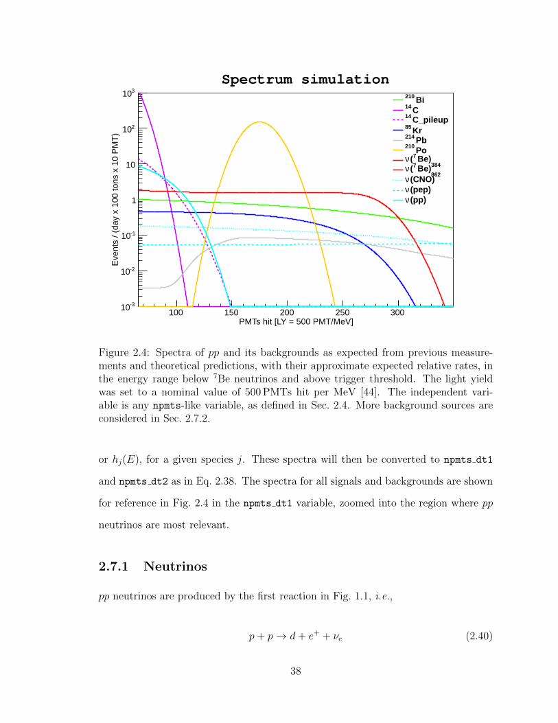
Figure 2.4: Spectra of pp and its backgrounds as expected from previous measure-ments and theoretical predictions, with their approximate expected relative rates, inthe energy range below 7Be neutrinos and above trigger threshold. The light yieldwas set to a nominal value of 500 PMTs hit per MeV [44]. The independent vari-able is any npmts-like variable, as defined in Sec. 2.4. More background sources areconsidered in Sec. 2.7.2.

or hj(E), for a given species j. These spectra will then be converted to npmts dt1

and npmts dt2 as in Eq. 2.38. The spectra for all signals and backgrounds are shown

for reference in Fig. 2.4 in the npmts dt1 variable, zoomed into the region where pp

neutrinos are most relevant.

2.7.1 Neutrinos

pp neutrinos are produced by the first reaction in Fig. 1.1, i.e.,

p+ p→ d+ e+ + νe (2.40)

38

Energy [MeV]0 0.05 0.1 0.15 0.2 0.25 0.3 0.35 0.4

0

0.002

0.004

0.006

0.008

0.01

0.012

0.014

0.016

0.018

pp neutrino energy spectrum

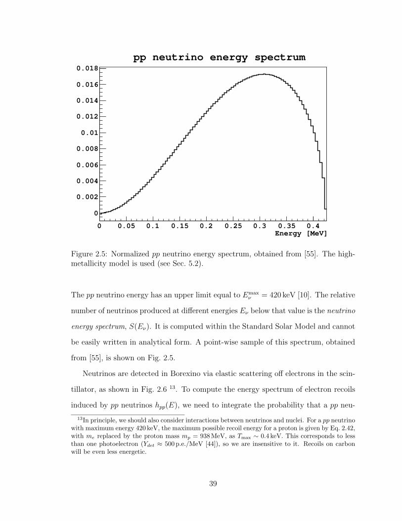
Figure 2.5: Normalized pp neutrino energy spectrum, obtained from [55]. The high-metallicity model is used (see Sec. 5.2).

The pp neutrino energy has an upper limit equal to Emaxν = 420 keV [10]. The relative

number of neutrinos produced at different energies Eν below that value is the neutrino

energy spectrum, S(Eν). It is computed within the Standard Solar Model and cannot

be easily written in analytical form. A point-wise sample of this spectrum, obtained

from [55], is shown on Fig. 2.5.

Neutrinos are detected in Borexino via elastic scattering off electrons in the scin-

tillator, as shown in Fig. 2.6 13. To compute the energy spectrum of electron recoils

induced by pp neutrinos hpp(E), we need to integrate the probability that a pp neu-

13In principle, we should also consider interactions between neutrinos and nuclei. For a pp neutrinowith maximum energy 420 keV, the maximum possible recoil energy for a proton is given by Eq. 2.42,with me replaced by the proton mass mp = 938 MeV, as Tmax ∼ 0.4 keV. This corresponds to lessthan one photoelectron (Ydet ≈ 500 p.e./MeV [44]), so we are insensitive to it. Recoils on carbonwill be even less energetic.

39

Figure 2.6: Neutrinos are detected in Borexino by elastic scattering off electrons inthe scintillator. The diagram on the left is known as neutral-current interaction,while that on the right is referred to as charged-current interaction. The fact thatthe charged-current interaction only occurs for electron-type neutrinos implies thatneutrino oscillations will alter the neutrino detection rate in Borexino. The diagramis from [33].

trino of energy Eν scatters off an electron, giving it energy E, over all Eν [4]:

hpp(E) dE = φ

∫ Emaxν

0

[S(Eν) dEν ]×(n

dσ

dE(Eν , E) dE

)(2.41)

where φ is the total neutrino flux produced in the Sun, S(Eν) is the energy spectrum

from the Standard Solar Model, n is the electron number density in the detector, and

dσ/dE(Eν , E) is the differential cross-section for a neutrino of energy Eν scattering

off an electron that recoils with energy E. From relativistic kinematics, the endpoint

of the pp-neutrino-induced electron recoil energy spectrum will be given by

Emax =2× Emax

ν

me + 2Emaxν

× Emaxν =

2× 420 keV

511 keV + 2× 420 keV× 420 keV = 261 keV (2.42)

where me is the electron mass. The value of Emax will be important when determining

which background species are relevant for our studies.

Although all pp neutrinos are produced as electron-type in the Sun, some of them

oscillate into other species by the time they are detected in Borexino (Sec. 1.3).

Electron-neutrinos can be detected through charged-current interactions as well as

40

neutral-current interactions, while muon- and tau-neutrinos can only be detected by

neutral-current interactions (see Fig. 2.6). This implies that the differential cross-

sections for neutrino-electron interactions are different for different neutrino flavors,

and we must weigh them by the probability that a neutrino is a certain flavor upon

arrival at the detector:

dσ

dE(Eν , E) = Pee(Eν)

dσedE

(Eν , E) + [1− Pee(Eν)]dσµ,τdE

(Eν , E) (2.43)

Pee is the energy-dependent survival probability, i.e., the probability for a neutrino

produced as electron type in the Sun to arrive at the detector as an electron neutrino.

The functional form for the differential cross-section can be obtained from [18].

The prescription for calculating the survival probability is given in [6, 56]. We can

thus calculate the differential cross-section of Eq. 2.43, and plug it into Eq. 2.41 to get

the neutrino-induced electron recoil energy spectrum hpp(E). The integral in Eq. 2.41

is approximated as a sum, for the neutrino energy spectrum is provided point-wise.

Using a spline interpolation between points reduces the error caused by the point-wise

approximation to negligible levels.

The procedure is very similar for three other neutrino species: pep, CNO, 7Be; it

has been previously described in further detail in [33]. The resulting recoil energy

spectra are in Fig. 2.4; hep and 8B neutrinos are ignored because of their exceedingly

small detection rates [15].

2.7.2 Backgrounds

In this section we discuss the various backgrounds present in Borexino, focusing on

the ones that affect the pp measurement most significantly. Unless otherwise noted,

β-decay and positron-emission endpoints and energy spectra, α- and γ-decay energies,

and Q-values were obtained from [57].

41

Reference Shape factor [MeV−1]Kuzminov/Osetrova [58] 1.24±0.04

Mortara et al. [60] 0.523±0.004Wietfeldt et al. [61] 0.64±0.04

Table 2.3: Summary of previous experimental results on the 14C spectral shape factor.For the present analysis, we use the result of Kuzminov/Osetrova, and explore theother two when studying systematic uncertainties (Sec. 4.6.6).

2.7.2.1 14C

14C is a β emitter that occurs as a natural isotope of carbon. Borexino was filled

with pseudocumene (C9H12) obtained from underground sources in which the relative

abundance of 14C is especially low. Nevertheless, the 14C rate decay rate in our

detector is approximately 40 Hz/100 t [33]. For reference, this is nearly five orders of

magnitude larger than the measured 7Be rate (∼45 cpd/100 t [14]), and it makes 14C

the most prominent source of background for the present analysis.

The β-decay energy spectrum of 14C can be written, without screening corrections,

as [58]

hno−screen14C (E) ∝ C14C(E)× p(E)E(E0 − E)2F (Z = 6, E) (2.44)

C14C(E) = [1 + βsf (E0 − E)] (2.45)

where p(E) is the (relativistic) momentum of an electron with energy E, E0 = 156 keV

is the endpoint of the 14C spectrum, F (Z,E) is known as the Fermi function and can

be calculated analytically [59], and βsf is a coefficient known as the shape factor, and

has to be measured experimentally. C14C(E) is known as the shape factor function.

A summary of previous such measurements is on Tab. 2.3. For the present analysis,

we use βsf = 1.24 MeV−1. We explore the effect of this choice in Sec. 4.6.6.

After the inclusion of screening corrections [59], Eq. 2.44 becomes

h14C(E) = ξ14CC14C(E)(E0 − E)2[(E − V0)2]1/2 (E − V0)F (Z = 6, E − V0) (2.46)

42

where V0 is an energy-dependent parameter that can be calculated. The normalization

constant ξ14C is such that the integral of the spectrum from 0 to E0 is 1.

2.7.2.2 Pile-up

As mentioned in Sec. 2.5, in the present study we use the energy estimators npmts dt1

and npmts dt2. These are computed by counting the number of PMTs registering

at least one photoelectron in a fixed time window (230 ns for npmts dt1, 400 ns for

npmts dt2) after the beginning of the cluster (that is, the reconstructed scintillation

event; see Sec. 2.3). Sometimes, a second physical event takes place within that

time window. The two events will be registered as a single event, which we call pile-

up. Because of its high rate, 14C is the component that generates the most pile-up.

However, all species can, in principle, create pile-up. Note that since two events are

taking place, the hit time distribution characteristic of pile-up events is different from

that of β-decays and electron recoils, where hits tend to arrive at the beginning of

the cluster window. Because α-decays also have longer-lived hit time distributions

(Sec. 2.1), we say pile-up events are α-like. We come back to this point in Sec. 4.2.

The spectral shape of 14C pile-up can be obtained by convolving the 14C energy

spectrum with itself. Because quenching is energy-dependent, the 14C spectrum must

be quenched before convolution. The convolved spectrum is then “de-quenched”, re-

sulting in a spectrum h14C pile−up(E); this can be converted to npmts dt1 or npmts dt2

using the prescription of Sec. 2.5.

The detector light yield in Borexino is known to depend on position [33]. Because

pile-up is generated by two events that can take place anywhere inside the Inner

Vessel (IV), as long as their overlap reconstructs inside the Fiducial Volume (FV),

the fiducial-volume-averaged detector light yield will be different for pile-up and single

scintillation events. To account for this, we must introduce a “relative light yield”,

43

which is an additional energy-independent quenching factor

Qpile−up(E) = Yrel Qβ(E) (2.47)

with Qβ(E) as in Eq. 2.3. This must be fed into Eq. 2.38 to calculate the final

Hpile−up(Np).

In Sec. 2.2 we mentioned that we need to select events within a Fiducial Vol-

ume (FV) to reduce backgrounds. Two 14C events occurring close in time but far

apart can potentially be reconstructed within the fiducial volume if they pile up.

This is a major difficulty in the present analysis, and we address it in Sec. 4.3.2.

We note that the relatively light yield Yrel may not be applicable to all the methods

described there.

2.7.2.3 Decay chains

There are three naturally occurring radioactive decay chains [62], known as the tho-

rium series, uranium series and actinium series. The Borexino collaboration made

very strong efforts for the reduction of the activities of all isotopes in these chains [38].

However, some radioactivity residue is responsible for background in our detector.

The uranium series can be seen in Tab. 2.4. Because of the extremely long half-life

of 238U (4.47×109 years), we could in principle expect the entire chain to be in secular

equilibrium, i.e., that all the isotopes decay with the same rate. However, we find

that the chain is broken in two places, at 222Rn and 210Pb, as we explain below. All

isotopes above 222Rn can be assumed to have rates below 1 cpd/100 t [38] and be in

secular equilibrium.

210Pb is often encountered out of secular equilibrium because of its relatively long

half-life (22 years) compared to the isotopes in the 222Rn section of the chain. With

a Q-value of 63.5 keV, 210Pb itself is not a problem, as it will lie underneath the

44

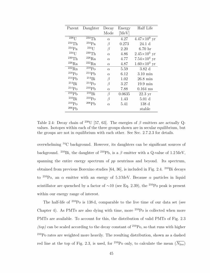
Parent Daughter Decay Energy Half LifeMode [MeV]

238U 234Th α 4.27 4.47×109 yr234Th 234Pa β 0.273 24.1 d234Pa 234U β 2.20 6.70 hr234U 230Th α 4.86 2.45×105 yr

230Th 226Ra α 4.77 7.54×104 yr226Ra 222Rn α 4.87 1.60×103 yr222Rn 218Po α 5.59 3.82 d218Po 214Pb α 6.12 3.10 min214Pb 214Bi β 1.02 26.8 min214Bi 214Po β 3.27 19.9 min214Po 210Pb α 7.88 0.164 ms210Pb 210Bi β 0.0635 22.3 yr210Bi 210Po β 1.43 5.01 d210Po 206Pb α 5.41 138 d206Pb stable

Table 2.4: Decay chain of 238U [57, 63]. The energies of β emitters are actually Q-values. Isotopes within each of the three groups shown are in secular equilibrium, butthe groups are not in equilibrium with each other. See Sec. 2.7.2.3 for details.

overwhelming 14C background. However, its daughters can be significant sources of

background. 210Bi, the daughter of 210Pb, is a β emitter with a Q-value of 1.2 MeV,

spanning the entire energy spectrum of pp neutrinos and beyond. Its spectrum,

obtained from previous Borexino studies [64, 36], is included in Fig. 2.4. 210Bi decays

to 210Po, an α emitter with an energy of 5.3 MeV. Because α particles in liquid

scintillator are quenched by a factor of ∼10 (see Eq. 2.39), the 210Po peak is present

within our energy range of interest.

The half-life of 210Po is 138 d, comparable to the live time of our data set (see

Chapter 4). As PMTs are also dying with time, more 210Po is collected when more

PMTs are available. To account for this, the distribution of valid PMTs of Fig. 2.3

(top) can be scaled according to the decay constant of 210Po, so that runs with higher

210Po rates are weighted more heavily. The resulting distribution, shown as a dashed

red line at the top of Fig. 2.3, is used, for 210Po only, to calculate the mean (Nlive)

45

and relative variance (vf ) of the live PMT distribution used in the calculation of the

response function in Eq. 2.38. The daughter of 210Po is 206Pb, which is stable.

Secular equilibrium in the uranium series is also broken by the diffusion of 222Rn,

a noble element with a half-life of 3.8 d, from detector materials -especially the nylon

vessels- into the scintillator. Its daughters 218Po, 214Pb, 214Bi, and 214Po have much

shorter half-lives and can be expected to be in secular equilibrium with 222Rn. We can

find the rate of all of these isotopes by looking for (and removing) delayed coincidences

between 214Bi and 214Po with 89% efficiency [36]. The resulting value will be used

in the analysis presented in Chapter 4 to fix the rate of 214Pb, a β-emitter whose

spectrum, shown in Fig. 2.4, has a shape obtained from previous studies [36]. We

neglect 222Rn, 218Po, and the remaining 11% of 214Bi-Po coincidences. We come back

to this assumption in Sec. 4.3.

The thorium series, shown in Tab. 2.5, is typically entirely in secular equilibrium,

as the only noble element, 220Rn, has a half-life of only 1 minute. Previous estimates

have indicated that the contribution from the entire chain is below 2 cpd/100 t [33],

which we can safely neglect.

The natural abundance of 235U, the parent isotope of the actinium series, is 0.7%

of the natural abundance of 238U. As the activity of 238U in Borexino is less than

1 cpd/100 t [38], we can neglect the contributions from the actinium series.

2.7.2.4 Other isotopes

In this section we list a number of isotopes not belonging to any of the naturally

occurring decay chains that have been found to be potential sources of background

in Borexino.

85Kr is a β emitter with a Q-value of 687 keV, relevant in the energy region of the

pp recoil spectrum. Its shape [65] is included in Fig. 2.4 and its rate will be extracted

from the data by spectral fitting.

46

Parent Daughter Decay Energy Half LifeMode [MeV]

232Th 228Ra α 4.08 1.41×1010 yr228Ra 228Ac β 0.0459 5.75 yr228Ac 228Th β 2.12 6.25 hr228Th 224Ra α 5.52 1.91 yr224Ra 220Rn α 5.79 3.63 d220Rn 216Po α 6.40 55.6 s216Po 212Pb α 6.91 0.145 s212Pb 212Bi β 0.570 10.6 hr

212Bi212Po β 64.06% 2.25

60.6 min208Tl α 35.94% 6.21212Po 208Pb α 8.96 299 ns208Tl 208Pb β 5.00 3.05 min208Pb stable

Table 2.5: Decay chain of 232Th [57, 63]. The energies of β emitters are actuallyQ-values. See Sec. 2.7.2.3 for details.

39Ar, a β emitter with a Q-value of 565 keV, is detected with a rate of

∼0.4 cpd/100 t [33] and we thus ignore it.

40K, a β emitter with a Q-value of 1.3 MeV was previously deemed a danger-

ous source of background. Its detection rate in Borexino has since been limited to

<0.4 cpd/100 t [13] and can be neglected.

87Rb, another β emitter, was not previously considered in Borexino, but recent

updates by the CNO neutrino analysis group have shown that this isotope could be

relevant in the energy range of interest for pp. 87Rb has a Q-value of 283.3 keV, very

similar to the endpoint of the pp-induced electron-recoil energy spectrum (261 keV,

from Eq. 2.42). The spectral shape of 87Rb is similar to the one of 14C, shown in

Eq. 2.46, albeit with a different shape factor function [66]:

h87Rb(E) = ξ87RbC87Rb(E)(E0−E)2[(E − V0)2]1/2 (E−V0)F (Z = 37, E−V0) (2.48)

47

Isotope Ac [ppm] Ai t1/2 [y]87Rb 60 28% 4.75×1010

40K 15000 0.012% 1.277×109

Table 2.6: Crustal abundance Ac, isotopic abundance Ai and half-life t1/2 of 87Rb and40K. The crustal abundances correspond to the elements Rb and K, not the particularisotopes. All data from [67]. Alternative bibliography was considered, with similarresults.

The crustal abundances, natural isotopic abundances and half-lives of 87Rb and 40K

are shown on Tab. 2.6. We can then calculate the ratio between the natural activities

of 87Rb and 40K as

A(87Rb)

A(40K)=

t40K1/2

t87Rb1/2

× N(87Rb)

N(40K)=

t40K1/2

t87Rb1/2

× N(Rb)Ai(87Rb)

N(K)Ai(40K)=t40K1/2Ac(Rb)Ai(87Rb)

t87Rb1/2 Ac(K)Ai(40K)

≈ 1

4

(2.49)

where A is the natural activity and N is the natural total number of atoms. Since

both K and Rb are alkali metals, we expect that their relative proportions remain the

same during purification. Under this assumption (which we scrutinize in Sec. 4.6.10),

and knowing that A(40K) < 0.4 cpd/100 t [13], we can estimate the upper limit of the

detection rate of 87Rb in Borexino to be

A(87Rb) < 0.1 cpd/100 t (2.50)

138La decays 34% of the time as a β-emitter with a Q-value of 1.0 MeV, and 66%

of the time by electron-capture, with a Q-value of 1.7 MeV. Due to its extremely small

isotopic abundance (0.09%) and long half-life (1.0×1011 years), we believe that it is

negligible. Studies are ongoing to justify this assumption.

All the backgrounds described so far pertain to the bulk of the scintillator. How-

ever, detector materials surrounding the inner detector, such as the nylon vessels, end

caps, photomultipliers and stainless steel sphere, can contain higher levels of back-

48

ground. We address these sources by applying a fiducial volume cut, as was done in

previous analyses [36].

2.7.2.5 Muons and cosmogenic isotopes

Muons traversing the Borexino detector can produce radioactive isotopes through

spallation processes. A very detailed description of all the backgrounds produced by

muons can be found in [44]. We exclude muons from our data sample with very high

efficiency [41]. We then exclude all data collected for a period of time after muons

cross the detector, to eliminate potential long-lived isotopes produced by the muons.

These adjustments of the data sample will be described in Sec. 4.2.

2.8 Spectral fitter

To extract the rates of neutrino signals and backgrounds from the data, a tool named

spectral-fitter was developed in the context of the 7Be analysis [14]. This tool was

then edited independently for the pep analysis [13]. We have now created a unified

tool for all the Borexino analysis groups, including the features of both previous

versions and new updates.

The fitter takes, as inputs:

• A list of signal and background species, j

• Initial guesses for the rates of all species, Rj

• Initial guesses for some input parameters ~v, which includes parameters related

to the energy response and resolution (Ydet, σped, vT0 ; see Eq. 2.38) and to the

relative quenching of α emitters and pile-up (Yα, Yrel; see Eqs. 2.39 and 2.47)

• Other physical parameters, such as Birks’ constant kB (Sec. 2.5), the 14C shape

factor βsf (Sec. 2.7.2.1)

49

• (Optional) Those parameters described in Secs. 2.8.2 and 2.8.3.

Any of the input parameters can optionally be fixed by the user; the rest are left free

to be varied by the fitter.

At every step in the fitting process, the fitter converts the energy spectra into

normalized spectra in the Np variable Hj(Np) as in Sec. 2.5, with the current values

of ~v, and calculates a total spectral function given by

H(Np;~v, Rj) =∑j

Hj(Np;~v)Rj (2.51)

where we have inserted an explicit dependence on ~v. Using that total spectral func-

tion, it then computes the likelihood for the current set of rates Rj, as

L(~v, Rj) =

Nbins∏i=1

exp [−H(Npi ;~v, Rj)] [H(Npi ;~v, Rj)]diΓ(di + 1)

(2.52)

where Nbins is the number of bins in the data histogram, Npi is the value of Np at bin

i, and di is the value of the data spectrum at bin i. Note that, because the Gamma

function is a generalization of the factorial function, this is the product of the Poisson

probability, for each bin, that the number of counts in that bin is detected given the

value expected from the analytical function. The fitter then modifies the values of

Rj and ~v within ranges specified by the user, until it finds the values that maximize

the likelihood L.

This basic operation of the fitter is modified in a number of cases, as described

below. We also discuss some important features that have been implemented in

spectral-fitter since it became an official tool in the Borexino collaboration. For

simplicity of notation, we omit the explicit dependence on Rj and ~v for the remain-

der of this section.

50

2.8.1 simulator

The most basic tool provided by the spectral-fitter package is simulator. This

tool generates mock signal and background spectra in the energy variable of inter-

est, for given light yield and β resolution parameters. Fig. 2.4 was generated with

simulator. We can additionally generate “fake” events by drawing random numbers

from the corresponding distributions.

2.8.2 Dark noise convolution

We define as Dark Noise (DN) all photomultiplier (PMT) hits that are registered

without arising from a physical event. The causes of these hits, among which is

intrinsic electronic noise in the PMTs, are explored in [36]. In the past, the DN

rate has been on the order of 15 hits for every 16-µs acquisition gate. This amounts

to an average of 0.2 hits for every 230-ns time window during which npmts dt1 is

calculated. In past analyses, this number of hits was negligible, but for the pp study,

with lower energies, this could be significant.

We have mitigated this problem in two ways. First, for Echidna Cycle 16 (see

Sec. 2.3), we have excluded the PMTs that produced the most noise, thereby reducing

the light yield but also the DN significantly. The current average number of DN hits

per 230-ns window is ∼0.07 14.

The second and complementary way in which we handle DN is by convolving

the measured DN spectrum with the analytically calculated spectra for signal and

backgrounds in spectral-fitter. To see how this is implemented, it is convenient

14This is a reduction of over 50%; at the same time, the number of live PMTs has reduced to∼1700 (see Fig. 2.3), which is a reduction of at most 15% from the nominal 2000 PMTs.

51

to rewrite the likelihood in Eq. 2.52 as the negative log-likelihood 15:

− lnL =

Nbins∑i=1

[H(Npi)− di lnH(Npi) + ln Γ(di + 1)] (2.53)

If we now want to take dark noise into consideration, we have to re-define each single

spectral function Hj(Np) as

HDNj (Np) =

∞∑n=0

pnHj(Np − n) (2.54)

where pn is the probability of measuring n DN hits in a 230-ns time window, so that

Eq. 2.51 is replaced by

HDN(Np) =∑j

HDNj (Np) =

∑j

∞∑n=0

pn Hj(Np − n) (2.55)

=∞∑n=0

pn∑j

Hj(Np − n) =∞∑n=0

pnH(Np − n)

Hj(Np) ≡ Hj(Np)Rj

and Eq. 2.53 can be rewritten as

− lnLDN =

Nbins∑i=1

[HDN(Npi)− di lnHDN(Npi) + ln Γ(di + 1)

](2.56)

=

Nbins∑i=1

[(∞∑n=0

pnH(Npi − n)

)− di ln

(∞∑n=0

pnH(Npi − n)

)+ ln Γ(di + 1)

]

The fitter then seeks to minimize this dark-noise-convolved function. The probabil-

ity distribution function for dark noise hits pn is approximated as the npmts win1

spectrum defined in Sec. 2.4 (for Np=npmts dt1; if Np=npmts dt2, the analogous

npmts win2 spectrum is used). We truncate the summation over n at some “dark

noise threshold”, above which we believe the npmts win1 spectrum contains real sig-

15We remove the explicit dependence of H(Np) on ~v and Rj for a more concise notation.

52

nal and background events, not dark noise. The dark noise threshold is an input

parameter of the fit.

2.8.3 Penalty method

Some of the species included in our fit will have rates that are known with some

precision. For example, the 7Be rate was measured previously by Borexino [14], and

we would like to constrain its rate in the fit such that it doesn’t stray too far from the

expected value. Fixing the rate is an option, but it would not account for possible

errors in the previous measurement. We account for this by including a penalty factor.

The likelihood is modified by adding an extra term:

∆ (− lnL) =∑s

[1

2

(Rs −Rspen

σspen

)2

+1

2ln(2πσ2

spen)

](2.57)

where the sum goes over all the species for which we apply a penalty factor, Rs is the

rate estimate for species s coming from the fit, Rspen is the a priori estimate of the

rate of this species, and σspen is the a priori estimate of the standard deviation of the

rate of species s. Thus, the fitter is biased to choose the central value input by the

user, but can alternatively choose another value if the penalty is compensated by a

better fit.

53

Chapter 3

Monte Carlo Simulations

The Borexino collaboration employs a simulation package named bxmc. It is composed

of two main parts: g4bx and bx elec. g4bx is an implementation of the Monte

Carlo (MC) simulation package Geant4 [68]. The user inputs the types of physical

processes desired, as well as certain detector conditions. The physics events are

simulated, resulting in energy depositions by various particles inside the Borexino

detector. Those energy depositions are then converted into light output based on

the properties of the scintillator, and propagated outward from the interaction point.

The light propagated is reflected by the surfaces of the detector; the output of g4bx

contains information about photons hitting individual PMTs.

bx elec is a custom-designed software that takes as input the photons hitting

the PMTs from g4bx and simulates the PMT response, including quantum efficiency,

dark hits, and other electronics effects, as well as triggering. This package is also

responsible for turning off invalid PMTs following the time-dependent distribution of

live PMTs in the data. The output file simulates exactly the format received from

the detector.

54

In Sec. 3.1 we describe the process that we went through to validate the simulation

package for the pp analysis. Both simulation packages have been previously described

in detail in [36].

3.1 Validation of the simulation package

The bxmc package was previously tuned for the 7Be and pep analyses [14, 13]. Calibra-

tion sources inserted in Borexino were used for generating events of known energies.

These were then mapped to corresponding values of the energy variable of choice

by looking at reconstructed data. Finally, events were generated in bxmc and sent

through the entire chain, ending with reconstructed physical events that need to

match the real data in the energy variable of choice. Input parameters of the fitter

such as the light yield and the kB parameter of the scintillator are varied until the

data and the MC match, both in energy and in hit time distribution.

The calibration sources used in the past are higher in energy than the events

expected from pp neutrinos. Therefore, we had to re-do calibration of the MC with

lower-energy sources. Since a full re-calibration would have taken a very long time,

we tuned the parameters so that MC and data match in our energy range of interest,

without attention to what happens at higher energies.

Four sources were used for the new MC tuning: 14C, 57Co, 139Ce and 203Hg. 14C

is a β emitter that is naturally present in the scintillator, while the other three are γ

emitters that were inserted into Borexino during the calibration campaign in 2009 [54].

Tab. 3.1 shows the different calibration sources, together with their energies and half-

lives. The next two sections deal separately with the treatment of energy and hit

time tuning.

Unfortunately, at the end of the tuning processed, we discovered that the MC

package did not include a 14C shape factor (see Sec. 2.7.2.1). The effect is relatively

55

Isotope Type Energy [keV] t1/214C β ≤156 5730 y57Co γ 122 272 d139Ce γ 166 138 d203Hg γ 279 47 d

Table 3.1: List of isotopes used for tuning the Monte Carlo package bxmc at theenergies relevant to the pp analysis. β decays occur at a range of energies going from0 to an endpoint energy, which is shown here. In the case of the γ sources, the energyshown is that of the most common γ line, which doesn’t occur in 100% of the decays.14C is naturally present in the scintillator, while the other three isotopes were insertedinto Borexino during a calibration campaign [54]. Isotope information from [57]. Toconvert energies to npmts dt1, note that the light yield is on the order of 500 PMTshit per MeV [44].

small, but might alter the tuning somewhat, so that all subsequent mention of MC

simulation of 14C β decays (see Chapter 4) should be interpreted as approximate.

Fortunately, none of our analysis relies on the MC simulations of 14C the tuning of

the soft α/β cut of Sec. 4.2 was done on the 7Be simulations.

3.1.1 Energy tuning

We first tackled the problem of reproducing with MC the part of the energy spectrum

that is due to 14C decays in the scintillator. MC was produced for a variety of values

of kB and light yield (Yscint). We wrote a program to do the comparison. It reads

a single run of data within the range of runs produced for the Monte Carlo. It then

normalizes the npmts distributions of the data and the MC such that the integral in

the range npmts=(45,65) is equal to 1. Finally, it computes bin-by-bin for data and

MC the following estimator:

eMC =65∑

npmts=45

(D −MD

)2

(3.1)

This gives a value for each estimator for each (Yscint,kB) pair, so we then make a 2D

colored plot and see where the minimum is for both estimators. We did this study

56

dividing the data in shells starting at the center and moving outward, so we could

see variations in radius.

We chose values of kB at intervals of 0.0005 cm/MeV between 0.0089 cm/MeV

and 0.0119 cm/MeV. We found that the match was moderate to good in the range

0.0099-0.0109 cm/MeV, and bad outside that range. In addition, we found that the

Yscint that minimizes eMC is not a constant value, but a function of the radius. We

implemented that function in g4bx, for all three values of kB, and re-generated the

MC. After that, we compared the three values to try and find the best match. Fig. 3.1

shows the results.

The graphs show that the match is relatively good for all three values in our

region of interest, with a slight improvement in the two higher values. More statistics

would be needed in the MC to make any claims about the match in the tail of the

distribution.

Next, we looked at the match between simulations and data in the case of cal-

ibration sources. We studied the same three values of kB as used before: 0.0099,

0.0104, 0.0109 (cm/MeV). As for Yscint, we tried the position-dependent functions,

as well as a fixed value of 17250 photons/MeV, which was the position-independent

value that resulted in the best match for 14C events. The sources were analyzed at

various positions. The results do not consistently favor a single configuration.

In what follows,

χ2/NDF =1

Nbins

∑npmts

(D −MσD

)2

(3.2)

where D and M represent the number of events at a given value of npmts for data

and Monte Carlo, respectively, and Nbins is the number of bins in the range we are

studying. This χ2/NDF is calculated for a given source at a given position. If you

take the sum of the χ2/NDF for all of the sources and positions for a given (kB,Yscint)

pair, the values are as shown on Tab. 3.2. Below we make a series of observations

and show example plots, to motivate our final decision.

57

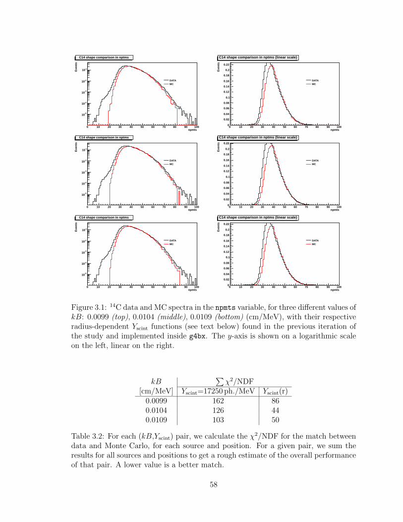
npmts0 10 20 30 40 50 60 70 80 90 100

Eve

nts

-510

-410

-310

-210

-110

DATAMC

C14 shape comparison in nptms

npmts0 10 20 30 40 50 60 70 80 90 100

Eve

nts

0

0.02

0.04

0.06

0.08

0.1

0.12

0.14

0.16

0.18

0.2

0.22

DATAMC

C14 shape comparison in nptms (linear scale)

npmts0 10 20 30 40 50 60 70 80 90 100

Eve

nts

-510

-410

-310

-210

-110

DATAMC

C14 shape comparison in nptms

npmts0 10 20 30 40 50 60 70 80 90 100

Eve

nts

0

0.02

0.04

0.06

0.08

0.1

0.12

0.14

0.16

0.18

0.2

0.22

DATAMC

C14 shape comparison in nptms (linear scale)

npmts0 10 20 30 40 50 60 70 80 90 100

Eve

nts

-510

-410

-310

-210

-110

DATAMC

C14 shape comparison in nptms

npmts0 10 20 30 40 50 60 70 80 90 100

Eve

nts

0

0.02

0.04

0.06

0.08

0.1

0.12

0.14

0.16

0.18

0.2

0.22

DATAMC

C14 shape comparison in nptms (linear scale)

Figure 3.1: 14C data and MC spectra in the npmts variable, for three different values ofkB: 0.0099 (top), 0.0104 (middle), 0.0109 (bottom) (cm/MeV), with their respectiveradius-dependent Yscint functions (see text below) found in the previous iteration ofthe study and implemented inside g4bx. The y-axis is shown on a logarithmic scaleon the left, linear on the right.

kB∑χ2/NDF

[cm/MeV] Yscint=17250 ph./MeV Yscint(r)0.0099 162 860.0104 126 440.0109 103 50

Table 3.2: For each (kB,Yscint) pair, we calculate the χ2/NDF for the match betweendata and Monte Carlo, for each source and position. For a given pair, we sum theresults for all sources and positions to get a rough estimate of the overall performanceof that pair. A lower value is a better match.

58

• The preferred value never corresponds to Yscint=17250 ph./MeV; in other words,

radius-dependent Yscint is always preferred.

• The test of Tab. 3.2 favors the two higher values of kB.

• Closest to the center, kB=0.0099 cm/MeV performs considerably worse than

the other two. For reference, in Fig. 3.2 we can see all three values of kB, with

variable light yield, for 139Ce source located at 12 cm from the center of the

detector.

• For all locations of 203Hg with |z| < 1.67 m (important for Fiducial Volume de-

termination; see Chapter 4), kB=0.0109 cm/MeV is never the preferred choice.

It is never disfavored too strongly with respect to the others.

• There are no significant overall correlations between the preferred value of kB

and the position or energy of the events 1.

• The match for 203Hg at the center is relatively bad for all values of kB and

Yscint. In Fig. 3.3 we see the best match, which is for kB=0.0104 cm/MeV. The

centers of the distributions match roughly, but the peaks are different in shape.

All in all, considering our choice of FV for this analysis (see Chapter 4), we

believe that the best match is kB = 0.0104 cm/MeV 2 with radius-dependent Yscint.

We encourage to continue to look at kB = 0.0109 cm/MeV in future studies, though,

as a preference for that value outside our FV was observed.

1All in all, 6 runs prefer kB=0.0099 cm/MeV (always followed relatively closely by one of theother two), 8 runs prefer kB=0.0104 cm/MeV, and 10 runs prefer kB=0.0109 cm/MeV (6 of themwith |z| > 1.67 m).

2Note that this value will be used for MC generation; it is not necessarily equal to the physicalvalue that is used for converting energy spectra to Borexino energy estimators (Sec. 2.5).

59

nnpmts30 40 50 60 70 80 90 100

0

0.005

0.01

0.015

0.02

0.025

0.03

0.035

0.04 Ce139Run010565

Data

MC

/NDF = 569/612Χ

KS Prob. 0

NNPMTS

nnhits30 40 50 60 70 80 90 100

0

0.005

0.01

0.015

0.02

0.025

0.03

0.035

0.04

Ce139Run010565

Data

MC

/NDF = 565/612Χ

KS Prob. 0

NNHITS

time (ns)0 200 400 600 800 1000 1200 1400 1600

-510

-410

-310

-210

Ce139Run010565

Data

MC

/NDF = 2.43e+03/14002Χ

KS Prob. 0

Clustered Hit Time all Lg

time (ns)0 10 20 30 40 50 60

0.01

0.02

0.03

0.04

0.05Ce139Run010565

Data

MC

/NDF = 2.31e+03/13952Χ

KS Prob. 0

Rec Time all Lg

nnpmts30 40 50 60 70 80 90 100

0

0.005

0.01

0.015

0.02

0.025

0.03

0.035

0.04 Ce139Run010565

Data

MC

/NDF = 101/602Χ

KS Prob. 1.06e-08

NNPMTS

nnhits30 40 50 60 70 80 90 100

0

0.005

0.01

0.015

0.02

0.025

0.03

0.035

0.04

Ce139Run010565

Data

MC

/NDF = 116/592Χ

KS Prob. 8.7e-09

NNHITS

time (ns)0 200 400 600 800 1000 1200 1400 1600

-510

-410

-310

-210

Ce139Run010565

Data

MC

/NDF = 2.65e+03/14342Χ

KS Prob. 0

Clustered Hit Time all Lg

time (ns)0 10 20 30 40 50 60

0.01

0.02

0.03

0.04

0.05Ce139Run010565

Data

MC

/NDF = 2.67e+03/14332Χ

KS Prob. 0

Rec Time all Lg

nnpmts30 40 50 60 70 80 90 100

0

0.005

0.01

0.015

0.02

0.025

0.03

0.035

0.04 Ce139Run010565

Data

MC

/NDF = 129/602Χ

KS Prob. 5.48e-11

NNPMTS

nnhits30 40 50 60 70 80 90 100

0

0.005

0.01

0.015

0.02

0.025

0.03

0.035

0.04

Ce139Run010565

Data

MC

/NDF = 142/592Χ

KS Prob. 2.34e-12

NNHITS

time (ns)0 200 400 600 800 1000 1200 1400 1600

-510

-410

-310

-210

Ce139Run010565

Data

MC

/NDF = 2.51e+03/14282Χ

KS Prob. 0

Clustered Hit Time all Lg

time (ns)0 10 20 30 40 50 60

0.01

0.02

0.03

0.04

0.05Ce139Run010565

Data

MC

/NDF = 2.37e+03/14202Χ

KS Prob. 0

Rec Time all Lg

Figure 3.2: Comparison between data and MC spectra in npmtsnorm (left) andnhitsnorm (right). Shown here are the data and Monte Carlo distributionsfor kB=0.0099 (top), 0.0104 (middle), 0.0109 (bottom) (cm/MeV), with radius-dependent Yscint, for 139Ce located 12 cm away from the center of the detector. Thethree sources closest to the center disfavor kB=0.0099 cm/MeV significantly, bothwith Yscint variable and Yscint fixed.

60

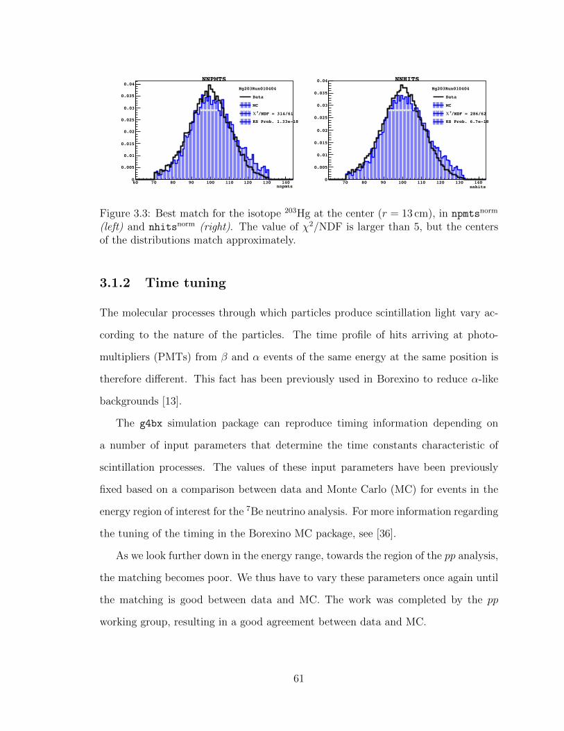
nnpmts60 70 80 90 100 110 120 130 1400

0.005

0.01

0.015

0.02

0.025

0.03

0.035

0.04Hg203Run010404

Data

MC

/NDF = 314/612Χ

KS Prob. 1.33e-18

NNPMTS

nnhits70 80 90 100 110 120 130 140

0

0.005

0.01

0.015

0.02

0.025

0.03

0.035

0.04

Hg203Run010404

Data

MC

/NDF = 286/622Χ

KS Prob. 6.7e-18

NNHITS

time (ns)0 200 400 600 800 1000 1200 1400 1600

-610

-510

-410

-310

-210

Hg203Run010404

Data

MC

/NDF = 3.47e+03/15152Χ

KS Prob. 0

Clustered Hit Time all Lg

time (ns)0 10 20 30 40 50 60

0.005

0.01

0.015

0.02

0.025

0.03

0.035

0.04Hg203Run010404

Data

MC

/NDF = 3.42e+03/15132Χ

KS Prob. 0

Rec Time all Lg

Figure 3.3: Best match for the isotope 203Hg at the center (r = 13 cm), in npmtsnorm

(left) and nhitsnorm (right). The value of χ2/NDF is larger than 5, but the centersof the distributions match approximately.

3.1.2 Time tuning

The molecular processes through which particles produce scintillation light vary ac-

cording to the nature of the particles. The time profile of hits arriving at photo-

multipliers (PMTs) from β and α events of the same energy at the same position is

therefore different. This fact has been previously used in Borexino to reduce α-like

backgrounds [13].

The g4bx simulation package can reproduce timing information depending on

a number of input parameters that determine the time constants characteristic of

scintillation processes. The values of these input parameters have been previously

fixed based on a comparison between data and Monte Carlo (MC) for events in the

energy region of interest for the 7Be neutrino analysis. For more information regarding

the tuning of the timing in the Borexino MC package, see [36].

As we look further down in the energy range, towards the region of the pp analysis,

the matching becomes poor. We thus have to vary these parameters once again until

the matching is good between data and MC. The work was completed by the pp

working group, resulting in a good agreement between data and MC.

61

Chapter 4

pp analysis

In this Chapter, we present the core of the work performed to extract the value of the

pp neutrino interaction rate from our data [69]. Sec. 4.1 deals with data selection. The

data are then further reduced by the cuts outlined in Sec. 4.2. In Sec. 4.3 we address

the backgrounds that make our measurement particularly challenging. Results are

presented in Sec. 4.4. Systematic uncertainties are studied in Sec. 4.5. In Sec. 4.6 we

present a review of further checks for systematic uncertainties.

4.1 Data Selection

Borexino Phase I encompassed 2007 thru 2011. The data collected during Phase I was

used for all the major analysis thus published by the collaboration [15, 14, 70, 13].

A detailed description of the hardware, methods and results of those analyses is

presented in [54, 36]. Since the beginning of 2012, Borexino has entered Phase II, with

reduced levels of some of the most prominent radiogenic backgrounds, most notably

85Kr, 210Bi and 210Po. This reduction is accomplished thanks to a series of successful

purification campaigns [36]. Due to a little-understood mistake in the purification

procedure, data acquired between mid-2010 and the end of 2011 is characterized by

high levels of 210Bi. As 210Bi is one of the main backgrounds to the detection of pp

62

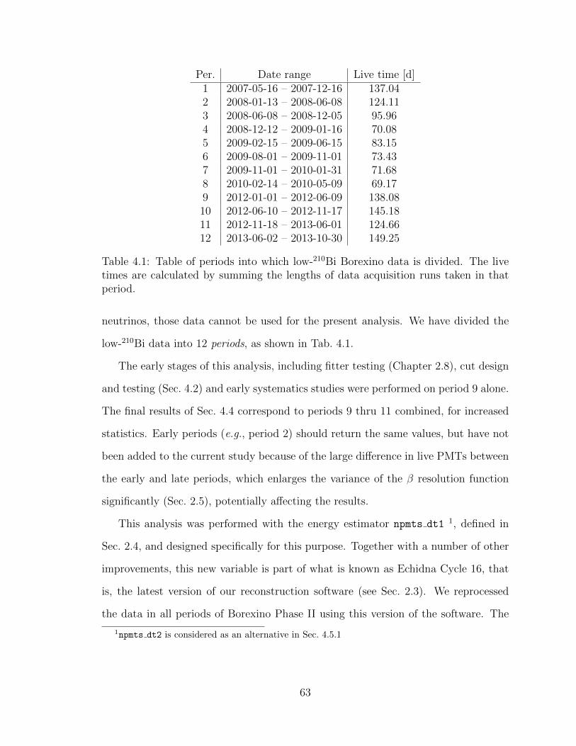
Per. Date range Live time [d]1 2007-05-16 – 2007-12-16 137.042 2008-01-13 – 2008-06-08 124.113 2008-06-08 – 2008-12-05 95.964 2008-12-12 – 2009-01-16 70.085 2009-02-15 – 2009-06-15 83.156 2009-08-01 – 2009-11-01 73.437 2009-11-01 – 2010-01-31 71.688 2010-02-14 – 2010-05-09 69.179 2012-01-01 – 2012-06-09 138.0810 2012-06-10 – 2012-11-17 145.1811 2012-11-18 – 2013-06-01 124.6612 2013-06-02 – 2013-10-30 149.25

Table 4.1: Table of periods into which low-210Bi Borexino data is divided. The livetimes are calculated by summing the lengths of data acquisition runs taken in thatperiod.

neutrinos, those data cannot be used for the present analysis. We have divided the

low-210Bi data into 12 periods, as shown in Tab. 4.1.

The early stages of this analysis, including fitter testing (Chapter 2.8), cut design

and testing (Sec. 4.2) and early systematics studies were performed on period 9 alone.

The final results of Sec. 4.4 correspond to periods 9 thru 11 combined, for increased

statistics. Early periods (e.g., period 2) should return the same values, but have not

been added to the current study because of the large difference in live PMTs between

the early and late periods, which enlarges the variance of the β resolution function

significantly (Sec. 2.5), potentially affecting the results.

This analysis was performed with the energy estimator npmts dt1 1, defined in

Sec. 2.4, and designed specifically for this purpose. Together with a number of other

improvements, this new variable is part of what is known as Echidna Cycle 16, that

is, the latest version of our reconstruction software (see Sec. 2.3). We reprocessed

the data in all periods of Borexino Phase II using this version of the software. The

1npmts dt2 is considered as an alternative in Sec. 4.5.1

63

other reconstruction code used in Borexino, Mach4, also had to be modified for this

analysis, and the data was also reprocessed with the latest version.

4.2 Cuts

A priori, we want to apply the same cuts employed in the 7Be analysis, which have

been tested and validated previously [14, 36]. However, some of those cuts are not

fit for our current purpose, and so we must be careful to eliminate them from our

analysis. The set of cuts used for the pp analysis, summarized very briefly in Tab. 4.3,

is:

• Muon and muon-daughter cuts: Candidate muon events tagged by the MTF,

MCR and IDF [41] trigger flags are eliminated from the sample. The IDF flag

is based on the event pulse shape. Since pile-up has a pulse shape that is,

in principle, not well understood, this cut could potentially be dangerous for

the pp analysis. Checks were made to ensure that it is not. Additionally, five

cuts known collectively as muon special, designed for the 7Be analysis [33], were

also employed in the pp analysis, after checking that they do not affect pile-up.

Events were vetoed if they occurred within a 0.3-s window after any muon, to

remove possible neutron captures and daughter isotope decays; 2 this results in

a live time adjustment and does not bias the sample.

• Trigger type cut: only trigger type 1 events with BTB input equal to 0 are

accepted (see Sec. 2.3), as they are the only events triggered by scintillation

events in the Inner Detector. Trigger type 1 events with BTB input 4 are

tagged as muons (MTF, see above). Trigger type 1 events with BTB input

64 are random triggers during the first few µs of which a scintillation event

2There could be other, longer-lived isotopes, that survive this cut. To test that hypothesis, wehave modified the cut to remove all events up to 5 s after muons. The variations of the results forthe pp rate were negligible.

64

occurred. We do not use them either for the estimation of dark noise or for the

analysis. The live time is adjusted accordingly. The triggering efficiency has

been studied in [36], and is ∼1 for events with npmts above ∼50.

• Clustering: We accept triggers with any non-zero number of clusters (Sec. 2.3).

Thus, if two clusters are separated by a time shorter than the time during

which we count PMTs hit (230 ns and 400 ns, respectively, for npmts dt1 and

npmts dt2), we accept the trigger and include some of the hits of the second

cluster in the energy estimators of the first cluster. The second cluster is not

subject to the triggering efficiency, so for consistency we study only the first

clusters. In addition, MOE must also see at least one cluster in the trigger,

for we apply certain cuts based on MOE variables (see below). Finally, both

Echidna and MOE must recognize the same number of clusters in the event 3.

The efficiency of this cut has been found to be extremely high at 7Be ener-

gies [36], and checked once again in the present study.

• Consistency of charge and hits: some events have previously been found that

have very small integrated charges compared to expectation based on the num-

ber of detected PMT hits [33]. These events are not well understood [36], so

for safety they are removed. In other words, if Q is the charge obtained by

integrating the PMT signals, and Qrec is the charge obtained by numerically

solving Eq. 2.13 for Npe (with cg = 0), we require that 0.6 < Q/Qrec < 1.6. The

efficiency of this cut has been found to be extremely high at 7Be energies [36],

and was once again checked in the present study.

3This cut is not quite justified, as MOE and Echidna have different clustering algorithms, andsometimes recognize the same physical event as containing different numbers of clusters. To study theeffect of this cut, we have looked at a data sample in which we make no requirement on the numberof clusters recognized by MOE (we remove the requirement that MOE sees a cluster altogether,thereby also removing cuts that require MOE variables). The results were not affected significantly.

65

• Mach4 strange events cut: we remove events with too many hits with invalid

charge [36]. Looking at period 11, we saw that only a few events were removed

by this cut; as this period contains ∼15 million evens, the efficiency adjustment

is insignificant.

• Cluster start time cut: the start time of a cluster within a trigger gate is deter-

mined by hardware. The RMS of the distribution is ∼50 ns [36]. We therefore

remove events that are more than a conservative 1.7µs from the programmed

time, as they may be caused by random noise or mis-labelled laser service trig-

gers (Sec. 2.3). A mistake in the data-taking procedure caused a relatively large

number of runs in period 11 to be lost due to this cut. The mistake was fixed

and the live time was adjusted accordingly.

• Crate fraction: There are 14 electronics racks in Borexino, each containing 160

channels, each in turn corresponding to a single PMT [33]. To exclude noise

coming from single racks, we remove events that have over 75% of their hits in

one rack. About 60 events were removed by this cut in period 11, so the live

time adjustment is negligible.

• Fiducial Volume cut: we keep events occurring in r < 3.021 m and |z| < 1.67 m,

as in the 7Be analysis. If two events pile up, the reconstructed position of the

resulting event might differ from both of the real positions of the scintillation

events. Thus, a FV cut will affect the pile-up distribution. We address this in

Sec. 4.3.2. In the 7Be analysis, uncertainty in the position reconstruction was

found to cause a 1% uncertainty in the determination of the FV. An expected

worsening of the position resolution at low energies as seen in Sec. 2.6 increases

our present effect to 2%. We include this in the systematics study of Sec. 4.5.

• Radon coincidences cut: we tag and remove events satisfying the conditions

outlined in Tab. 4.2, which are candidate 214Bi-Po coincidences. In periods 9

66

Time separation < 1.2 msSpatial separation < 1 mnpenorm of 1st event ∈ (90, 1800)npenorm of 2nd event ∈ (200, 500)

Table 4.2: List of conditions required for a candidate 214Bi-Po coincidence. The timeseparation upper limit is equal to five 214Po lifetimes. The npenorm cuts on the first andsecond events are designed to select candidate 214Bi and 214Po decays, respectively.See Sec. 2.7.2.3 for isotope details.

thru 11 combined, there were 5.0×107 events passing all cuts, of which 5.8×105

had npenorm ∈ (90, 1800), and 1.4×105 had npenorm ∈ (200, 500). The induced

dead exposure, then, is

DT222Rn = 5.8×105× 1.4× 105

5.0× 107×1.2 ms× 4

3π(1 m)3×0.88 t/m3 = 8.3×10−5 td

(4.1)

which is a negligible adjustment to our exposure (Tabs. 4.1 and 4.11). The

tagged events are also used to fix the 214Pb rate in the fit (Sec. 4.3). The

efficiency for this cut is 89% [36], and it is accounted for in the current study.

Additionally, we studied a soft α/β cut. Based on the Gatti parameter [36], we

can distinguish events that have longer or shorter hit time distributions. This energy-

dependent cut was tuned in our analysis based on MC: for each energy, we chose a

value of the Gatti parameter for which 1% of β-like events are missed as the threshold

between α-like and β-like. We must therefore adjust the final pp rate by 1%. This

cut is not employed in our analysis, but is used for a cross-check in Sec. 4.6.5.

Other cuts applied for the 7Be analysis were the Geometrical uniformity, Npeaks

and Spherical harmonics cuts. The Npeaks cut aims at tagging clusters that arise from

two separate scintillation events based on the time distribution of PMTs hit. To avoid

biasing our pile-up events, we do not apply this cut. The Geometrical uniformity

and Spherical harmonics cuts are based on the PMT hit position distributions of

67

Cut PurposeMuon/Daughters Remove muons and cosmogenic radioactive isotopesTrigger type Select events triggered by scintillation events in the inner detectorClustering Select triggers with only one scintillation event in the DAQ windowCharge vs. hits Remove events with possible electronic noise from PMT (in clusters)Strange events Remove events with possible electronic noise from PMT (in hits)Cluster time Select events that occurred at the preset time within trigger windowCrate fraction Remove events with possible noise from electronics rackFiducial Volume Remove external backgroundRn coincidences Tag and remove isotopes in the Radon branch of the Uranium seriesSoft α/β Remove α and pile-up events

Table 4.3: List of cuts employed in the pp analysis. See text for a more detaileddescription. The soft α/β cut is not employed in the analysis, but used to check forsystematic errors.

the events. Pile-up events will have PMT hit distributions that are not very well

understood, so we have decided not to apply those cuts.

Fig. 4.1 shows the event spectrum of Periods 9–11 (combined) in Borexino in

our variable of choice (npmts dt1), after applying all the cuts. The large bump

at low energies is due to 14C β decays, while the second most prominent peak at

npmts dt1∼150 is due to α decays of 210Po. pp neutrinos are expected in the valley

between the two features, as is pile-up (see Fig. 2.4).

The choice of the fit domain was optimized for the pp analysis. We wanted to

probe the lowest possible energies, in order to include as much of the 14C as we can.

By doing so, we improve the fit quality and we can also obtain a reliable estimate of

the 14C decay rate inside our detector. The trigger threshold K (Sec. 2.3) limits our

ability to push the fit region to very low energies. To determine our minimum possible,

we divided the full energy range in bins of width ∆npmts dt1=10. We calculated the

total count rate after cuts in each of those bins as a function of time, and looked for

the lowest bin that showed stability. We determined that we can perform fits with

starting points as low as npmts dt1=55. This leaves open the question of trigger

efficiency and dependence of position reconstruction on energy as possible sources of

68

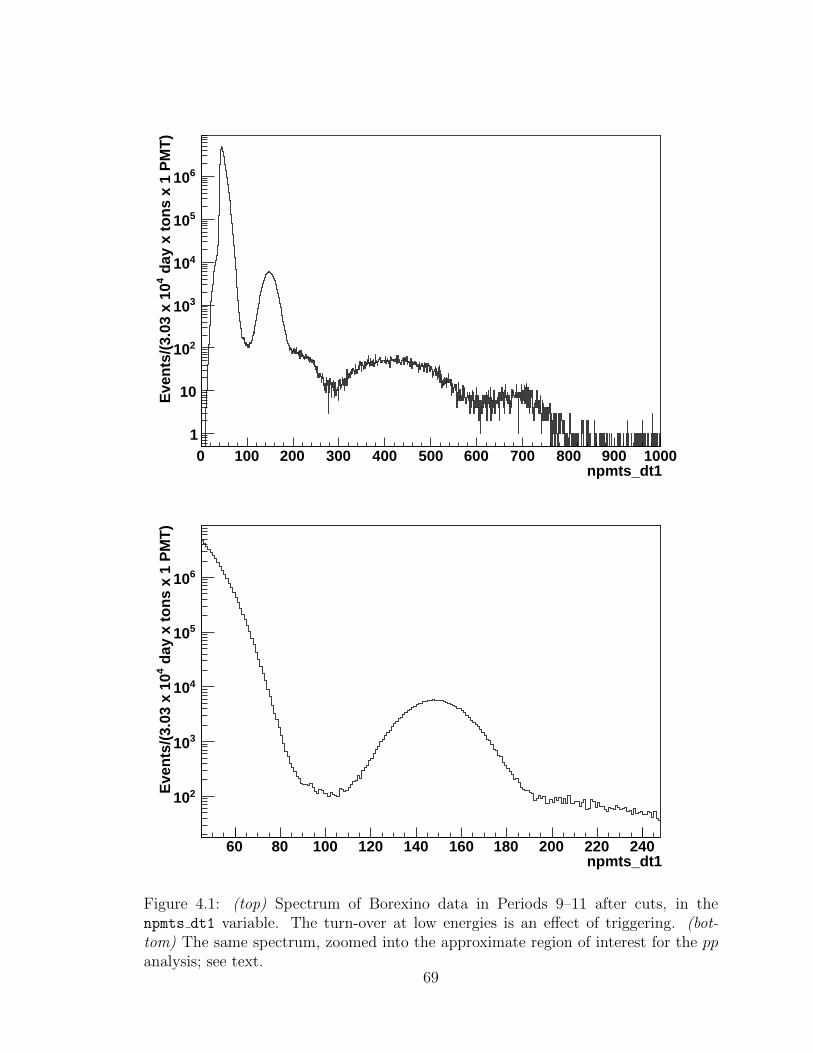
npmts_dt10 100 200 300 400 500 600 700 800 900 1000

day

x t

on

s x

1 P

MT

)4

Eve

nts

/(3.

03 x

10

1

10

210

310

410

510

610

npmts_dt160 80 100 120 140 160 180 200 220 240

day

x t

on

s x

1 P

MT

)4

Eve

nts

/(3.

03 x

10

210

310

410

510

610

Figure 4.1: (top) Spectrum of Borexino data in Periods 9–11 after cuts, in thenpmts dt1 variable. The turn-over at low energies is an effect of triggering. (bot-tom) The same spectrum, zoomed into the approximate region of interest for the ppanalysis; see text.

69

systematics when choosing a fit energy range. Those will be accounted by varying

the fit start point in Sec. 4.5.

As for the upper bound, the first consideration was that we wanted to include the

full pp-neutrino-induced electron-recoil spectrum (endpoint 261 keV, npmts dt1∼130;

see Sec. 2.7.1). That number falls within the 210Po peak, and so for increased fit

quality we decided to include the entire peak. The final upper bound of our fit region

is npmts dt1=220. Variations around that value are also considered in Sec. 4.5.

At the bottom of Fig. 4.1 is the data spectrum zoomed into the approximate

region of interest for this analysis.

4.3 Main backgrounds

The neutrino signals and backgrounds were discussed in Sec. 2.7. In the next sections

we explain how we tackle specific problems brought about by the two backgrounds

that are most challenging for the measurement of the pp neutrino interaction rate:

14C (Sec. 4.3.1) and pile-up (Sec. 4.3.2). 85Kr, 210Bi and 210Po are included in the fit,

with their rates (and relative quenching, in the case of 210Po) free to vary.

214Pb is included, with its rate fixed by looking for 214Bi-Po coincidences, as

explained in Sec. 2.7.2.3. In periods 9 thru 11 combined, we found 16 214Bi-Po

coincidences in the Fiducial Volume. After accounting for the 89% efficiency [36],

the rate for all of the isotopes in the uranium series between 222Rn and 214Po is

0.059 cpd/100 t. This justifies the assumption that 222Rn, 218Po and the untagged

11% of 214Bi-Po coincidences can be neglected 4.

Finally, pep, CNO and 7Be neutrinos are background sources in this measurement.

We fix the rates of pep and CNO neutrinos to their expected values from theory [13]:

2.80 cpd/100 t and 5.36 cpd/100,t, respectively. 7Be is left free with a penalty fac-

4We could potentially neglect 214Pb as well, but for historical reasons, and due to its abnormalshape (Fig. 2.4), we have included it.

70

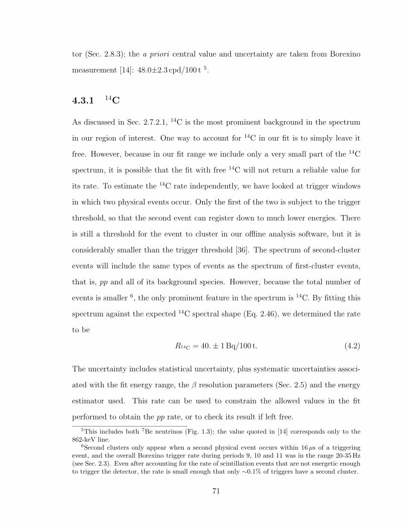
tor (Sec. 2.8.3); the a priori central value and uncertainty are taken from Borexino

measurement [14]: 48.0±2.3 cpd/100 t 5.

4.3.1 14C

As discussed in Sec. 2.7.2.1, 14C is the most prominent background in the spectrum

in our region of interest. One way to account for 14C in our fit is to simply leave it

free. However, because in our fit range we include only a very small part of the 14C

spectrum, it is possible that the fit with free 14C will not return a reliable value for

its rate. To estimate the 14C rate independently, we have looked at trigger windows

in which two physical events occur. Only the first of the two is subject to the trigger

threshold, so that the second event can register down to much lower energies. There

is still a threshold for the event to cluster in our offline analysis software, but it is

considerably smaller than the trigger threshold [36]. The spectrum of second-cluster

events will include the same types of events as the spectrum of first-cluster events,

that is, pp and all of its background species. However, because the total number of

events is smaller 6, the only prominent feature in the spectrum is 14C. By fitting this

spectrum against the expected 14C spectral shape (Eq. 2.46), we determined the rate

to be

R14C = 40.± 1 Bq/100 t. (4.2)

The uncertainty includes statistical uncertainty, plus systematic uncertainties associ-

ated with the fit energy range, the β resolution parameters (Sec. 2.5) and the energy

estimator used. This rate can be used to constrain the allowed values in the fit

performed to obtain the pp rate, or to check its result if left free.

5This includes both 7Be neutrinos (Fig. 1.3); the value quoted in [14] corresponds only to the862-keV line.

6Second clusters only appear when a second physical event occurs within 16µs of a triggeringevent, and the overall Borexino trigger rate during periods 9, 10 and 11 was in the range 20-35 Hz(see Sec. 2.3). Even after accounting for the rate of scintillation events that are not energetic enoughto trigger the detector, the rate is small enough that only ∼0.1% of triggers have a second cluster.

71

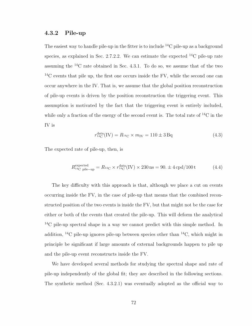
4.3.2 Pile-up

The easiest way to handle pile-up in the fitter is to include 14C pile-up as a background

species, as explained in Sec. 2.7.2.2. We can estimate the expected 14C pile-up rate

assuming the 14C rate obtained in Sec. 4.3.1. To do so, we assume that of the two

14C events that pile up, the first one occurs inside the FV, while the second one can

occur anywhere in the IV. That is, we assume that the global position reconstruction

of pile-up events is driven by the position reconstruction the triggering event. This

assumption is motivated by the fact that the triggering event is entirely included,

while only a fraction of the energy of the second event is. The total rate of 14C in the

IV is

rdata14C (IV) = R14C ×mIV = 110± 3 Bq (4.3)

The expected rate of pile-up, then, is

Rexpected14C pile−up = R14C × rdata

14C (IV)× 230 ns = 90.± 4 cpd/100 t (4.4)

The key difficulty with this approach is that, although we place a cut on events

occurring inside the FV, in the case of pile-up that means that the combined recon-

structed position of the two events is inside the FV, but that might not be the case for

either or both of the events that created the pile-up. This will deform the analytical

14C pile-up spectral shape in a way we cannot predict with this simple method. In

addition, 14C pile-up ignores pile-up between species other than 14C, which might in

principle be significant if large amounts of external backgrounds happen to pile up

and the pile-up event reconstructs inside the FV.

We have developed several methods for studying the spectral shape and rate of

pile-up independently of the global fit; they are described in the following sections.

The synthetic method (Sec. 4.3.2.1) was eventually adopted as the official way to

72

estimate pile-up in the pp analysis. Other methods are considered in the systematics

studies of Sec. 4.5.

4.3.2.1 Synthetic pile-up

As explained in Sec. 2.3, trigger windows are 16-µs long. By design, physical events

that trigger the detector occur near the beginning of trigger windows. For approx-

imately the first half of the trigger window, after-pulses from the PMTs can occur.

However, during the last ∼4µs of the trigger window, no more after-pulses occur, as

can be seen in Fig. 4.2, and hits arriving at the PMTs are uncorrelated with the event

that triggered the detector. If we randomly select a 230-ns-long time window within

that 4-µs time period, most of the time the 230-ns window chosen will contain no

or few hits, caused by dark noise. However, sometimes an event will have occurred

inside that time window; thus, if we overlap the selected window with the primary

event, we create artificial pile-up with a controlled method.

From the overlapped data set, we define as synthetic pile-up events those that,

when compared to their parent primary event, have a value of npmts dt1 that is at

least Nmin higher. The value of Nmin can be varied and for this analysis was set to

Nmin = 5 (in npmts dt1).

If we overlap exactly one 230-ns-long window from the end of the trigger with each

one of the primary events, we obtain a sample of synthetic pile-up that corresponds

to the exposure of data used. However, for increased statistics, we can repeat the

process by choosing n random, uncorrelated 230-ns windows for each of the triggers.

The final live time of the synthetic pile-up sample will be n times the live time of the

original data sample. We have chosen n = 4, as a compromise between statistics and

processing time.

Using this method, we can obtain the true rate and spectral shape of pile-up in

our detector. The rate is equal to the number of pile-up events created, divided by

73

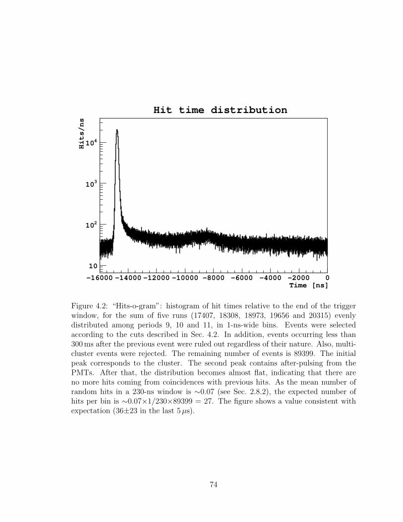
Time [ns]-16000 -14000 -12000 -10000 -8000 -6000 -4000 -2000 0

Hits/ns

10

210

310

410

Hit time distribution

Figure 4.2: “Hits-o-gram”: histogram of hit times relative to the end of the triggerwindow, for the sum of five runs (17407, 18308, 18973, 19656 and 20315) evenlydistributed among periods 9, 10 and 11, in 1-ns-wide bins. Events were selectedaccording to the cuts described in Sec. 4.2. In addition, events occurring less than300 ms after the previous event were ruled out regardless of their nature. Also, multi-cluster events were rejected. The remaining number of events is 89399. The initialpeak corresponds to the cluster. The second peak contains after-pulsing from thePMTs. After that, the distribution becomes almost flat, indicating that there areno more hits coming from coincidences with previous hits. As the mean number ofrandom hits in a 230-ns window is ∼0.07 (see Sec. 2.8.2), the expected number ofhits per bin is ∼0.07×1/230×89399 = 27. The figure shows a value consistent withexpectation (36±23 in the last 5µs).

74

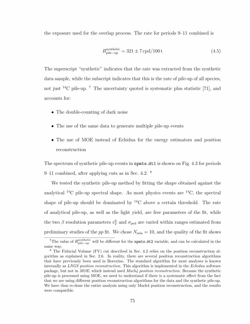
the exposure used for the overlap process. The rate for periods 9–11 combined is

Rsyntheticpile−up = 321± 7 cpd/100 t (4.5)

The superscript “synthetic” indicates that the rate was extracted from the synthetic

data sample, while the subscript indicates that this is the rate of pile-up of all species,

not just 14C pile-up. 7 The uncertainty quoted is systematic plus statistic [71], and

accounts for:

• The double-counting of dark noise

• The use of the same data to generate multiple pile-up events

• The use of MOE instead of Echidna for the energy estimators and position

reconstruction

The spectrum of synthetic pile-up events in npmts dt1 is shown on Fig. 4.3 for periods

9–11 combined, after applying cuts as in Sec. 4.2. 8

We tested the synthetic pile-up method by fitting the shape obtained against the

analytical 14C pile-up spectral shape. As most physics events are 14C, the spectral

shape of pile-up should be dominated by 14C above a certain threshold. The rate

of analytical pile-up, as well as the light yield, are free parameters of the fit, while

the two β resolution parameters v0T and σped are varied within ranges estimated from

preliminary studies of the pp fit. We chose Nmin = 10, and the quality of the fit shows

7The value of Rsyntheticpile−up will be different for the npmts dt2 variable, and can be calculated in the

same way.8 The Fiducial Volume (FV) cut described in Sec. 4.2 relies on the position reconstruction al-

gorithm as explained in Sec. 2.6. In reality, there are several position reconstruction algorithmsthat have previously been used in Borexino. The standard algorithm for most analyses is knowninternally as LNGS position reconstruction. This algorithm is implemented in the Echidna softwarepackage, but not in MOE, which instead used Mach4 position reconstruction. Because the syntheticpile-up is processed using MOE, we need to understand if there is a systematic effect from the factthat we are using different position reconstruction algorithms for the data and the synthetic pile-up.We have thus re-done the entire analysis using only Mach4 position reconstruction, and the resultswere compatible.

75

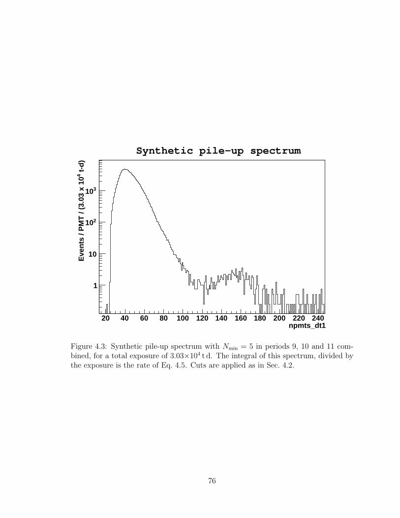
npmts_dt120 40 60 80 100 120 140 160 180 200 220 240

t-d

)4

Eve

nts

/ P

MT

/ (3

.03

x 10

1

10

210

310

Synthetic pile-up spectrum

Figure 4.3: Synthetic pile-up spectrum with Nmin = 5 in periods 9, 10 and 11 com-bined, for a total exposure of 3.03×104 t d. The integral of this spectrum, divided bythe exposure is the rate of Eq. 4.5. Cuts are applied as in Sec. 4.2.

76

3.7 PMT/MeV]±PMTs hit [LY = 390 60 70 80 90 100 110 120

Eve

nts

/ (d

ay x

100

to

ns

x 1

PM

T)

-310

-210

-110

1

Data from 30276.7 days x tons livetime

/ N-DOF = 11.419 / 382χTotal spectrum,

8.8 cpd/100 tons±C_pileup_q = 161 14

Figure 4.4: Synthetic pile-up spectrum with Nmin = 10 in periods 9, 10 and 11combined, fitted against the analytical 14C pile-up shape. The light yield shown hereis different from the one we find in the pp fit (Fig. 4.8), because pile-up can occurbetween events that take place anywhere in the IV, and the light yield is position-dependent.

that indeed, for that cutoff, the synthetic pile-up consists primarily of 14C pile-up, as

can be seen in Fig. 4.4. The relative light yield Yrel is fixed at 1, as 14C pile-up is the

only species in the fit, and thus the light yield found by the fitter will be the light

yield of 14C pile-up. The resulting rate of 14C pile-up in the synthetic data sample is

Rsynthetic14C pile−up = 161± 9 (stat)± 15 (syst) cpd/100 t, (4.6)

on the same order of magnitude as the expected value of Eq. 4.4. The expected

rate was based on assumptions about the position reconstruction algorithms that

were never tested; the present estimate is more reliable. Repeating the fit with the

77

synthetic data sample obtained with Nmin = 5 did not return a good χ2, probably

because of the inclusion of too much dark noise. The choice of Nmin for the pp analysis

is addressed in Sec. 4.6.1. The systematic uncertainty is dominated by the choice

of the β resolution parameters and the fit range. Note that Rsynthetic14C pile−up (Eq. 4.6) is

considerably lower than Rsyntheticpile−up (Eq. 4.5), as the latter includes pile-up of low-energy

noise events as well as signal and background events.

The spectral shape of synthetic pile-up (Fig. 4.3) can now be included as a new

background species in the spectral fit. No energy resolution is applied for this species,

which is already expressed in npmts dt1 and npmts dt2, the variables in which data

are presented. Only the rate can be a free parameter for synthetic pile-up.

We note that, because synthetic pile-up naturally includes dark noise, it should

be exempt from the treatment described in Sec. 2.8.2. However, because we imple-

mented dark noise convolution on the global spectral function (Eq. 2.56), we cannot

easily remove synthetic pile-up from the convolution. This has been found to have a

negligible effect on the final result.

4.3.2.2 npmts win1 convolution

Since pile-up is not really a background species, but rather a special effect caused by

the overlap of multiple species with each other, we consider the possibility of including

pile-up organically in the treatment of the other species, without resorting to an extra

species inserted into the fitter.

The spectrum of random triggers in the npmts win1 variable (see Sec. 2.4) can

be interpreted as the probability distribution function for the number of hits coming

from random events in a 230-ns time window. Fig. 4.5 shows the distribution, before

normalization. If we normalize this distribution and convolve it with each of the

analytical species included in the fitter 9, we will have included pile-up naturally in

9npmts win2 must be used instead of npmts win1 if the data are being represented in npmts dt2.

78

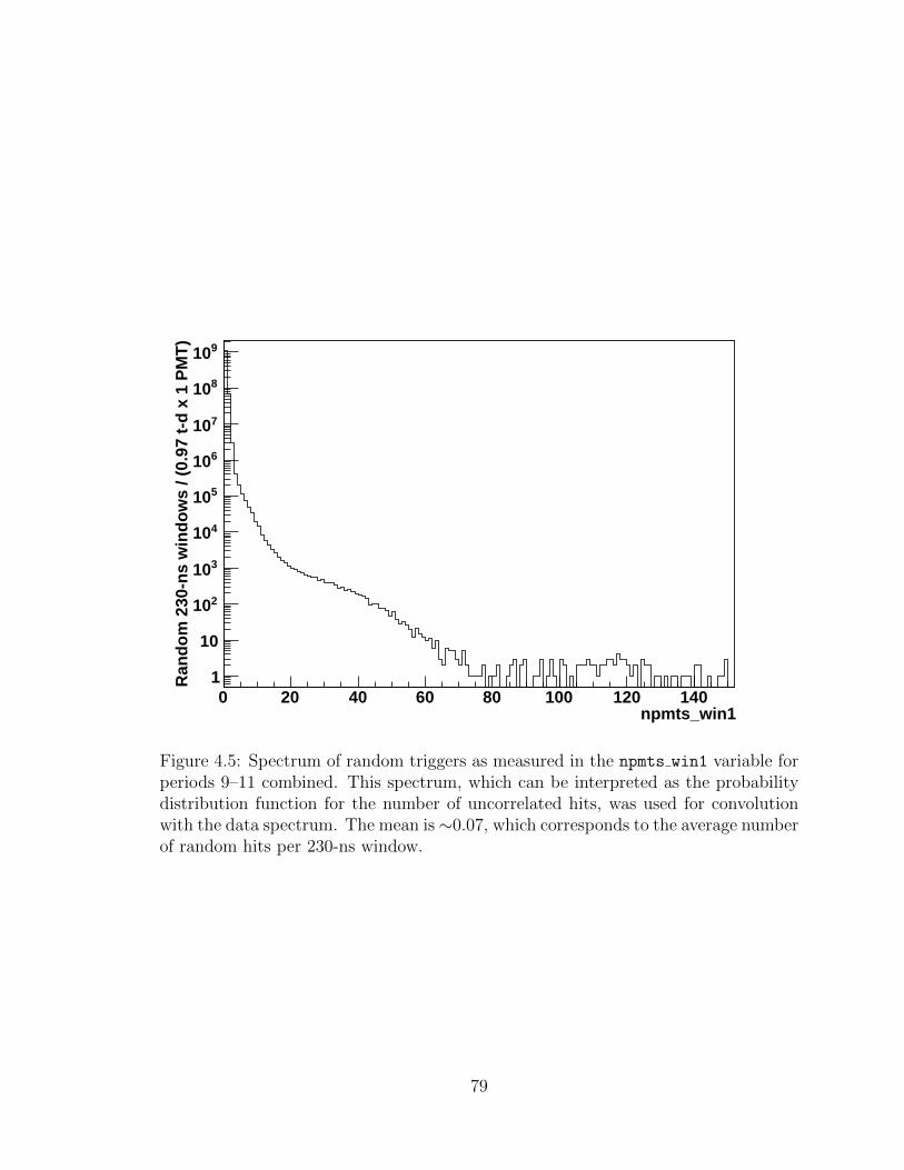
npmts_win10 20 40 60 80 100 120 140

Ran

do

m 2

30-n

s w

ind

ow

s / (

0.97

t-d

x 1

PM

T)

1

10

210

310

410

510

610

710

810

910

Figure 4.5: Spectrum of random triggers as measured in the npmts win1 variable forperiods 9–11 combined. This spectrum, which can be interpreted as the probabilitydistribution function for the number of uncorrelated hits, was used for convolutionwith the data spectrum. The mean is∼0.07, which corresponds to the average numberof random hits per 230-ns window.

79

PMTs hit [LY = 500 PMT/MeV]60 80 100 120 140 160 180 200 220

Eve

nts

/ (da

y x

100

tons

x 1

0 P

MT

)

-310

-210

-110

1

10

210

310Bi210

C14

Kr85

Pb214

Po210

384Be)7 (ν

862Be)7 (ν

(CNO)ν(pep)ν(pp)ν

Spectrum simulation

Figure 4.6: Spectra of pp and its backgrounds as expected from previous measure-ments and theoretical predictions, with their approximate expected relative rates, inour energy range of interest. We do not include pile-up as one of the backgroundspecies. Pile-up is accounted for by convolving all signal and background spectrawith the spectrum of random events, as described in Sec. 4.3.2.2. The effect is mosteasily visible in the tail of the 14C spectrum, which is deformed as compared to theone seen in Fig. 2.4.

our data sample. This procedure is described in Sec. 2.8.2 as a way to include dark

noise; here, we truncate the summation over n in Eq. 2.56 at npmts win1=100 to

include signal and background species as well as dark noise. The probability to get

more npmts win1>100 is (from the graph) 3×10−7, low enough that we can safely

cut off there.

To visualize the effect of this procedure, we repeat the simulation of Fig. 2.4, but

without the inclusion of 14C pile-up as a background species in the fit, and with the

convolution of random events up to npmts win1=100, in Fig. 4.6.

80

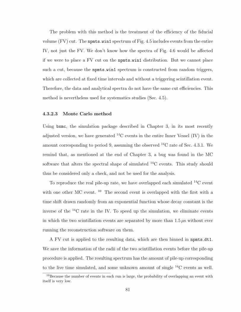
The problem with this method is the treatment of the efficiency of the fiducial

volume (FV) cut. The npmts win1 spectrum of Fig. 4.5 includes events from the entire

IV, not just the FV. We don’t know how the spectra of Fig. 4.6 would be affected

if we were to place a FV cut on the npmts win1 distribution. But we cannot place

such a cut, because the npmts win1 spectrum is constructed from random triggers,

which are collected at fixed time intervals and without a triggering scintillation event.

Therefore, the data and analytical spectra do not have the same cut efficiencies. This

method is nevertheless used for systematics studies (Sec. 4.5).

4.3.2.3 Monte Carlo method

Using bxmc, the simulation package described in Chapter 3, in its most recently

adjusted version, we have generated 14C events in the entire Inner Vessel (IV) in the

amount corresponding to period 9, assuming the observed 14C rate of Sec. 4.3.1. We

remind that, as mentioned at the end of Chapter 3, a bug was found in the MC

software that alters the spectral shape of simulated 14C events. This study should

thus be considered only a check, and not be used for the analysis.

To reproduce the real pile-up rate, we have overlapped each simulated 14C event

with one other MC event. 10 The second event is overlapped with the first with a

time shift drawn randomly from an exponential function whose decay constant is the

inverse of the 14C rate in the IV. To speed up the simulation, we eliminate events

in which the two scintillation events are separated by more than 1.5µs without ever

running the reconstruction software on them.

A FV cut is applied to the resulting data, which are then binned in npmts dt1.

We save the information of the radii of the two scintillation events before the pile-up

procedure is applied. The resulting spectrum has the amount of pile-up corresponding

to the live time simulated, and some unknown amount of single 14C events as well.

10Because the number of events in each run is large, the probability of overlapping an event withitself is very low.

81

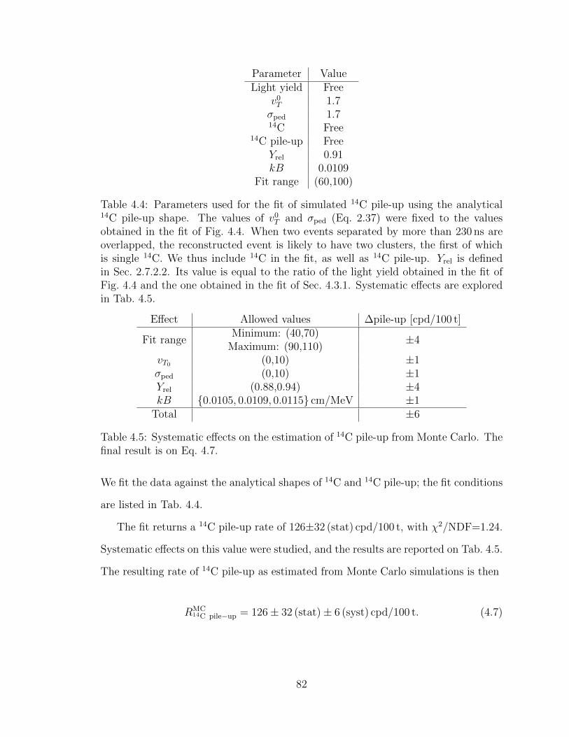
Parameter ValueLight yield Free

v0T 1.7

σped 1.714C Free

14C pile-up FreeYrel 0.91kB 0.0109

Fit range (60,100)

Table 4.4: Parameters used for the fit of simulated 14C pile-up using the analytical14C pile-up shape. The values of v0

T and σped (Eq. 2.37) were fixed to the valuesobtained in the fit of Fig. 4.4. When two events separated by more than 230 ns areoverlapped, the reconstructed event is likely to have two clusters, the first of whichis single 14C. We thus include 14C in the fit, as well as 14C pile-up. Yrel is definedin Sec. 2.7.2.2. Its value is equal to the ratio of the light yield obtained in the fit ofFig. 4.4 and the one obtained in the fit of Sec. 4.3.1. Systematic effects are exploredin Tab. 4.5.

Effect Allowed values ∆pile-up [cpd/100 t]

Fit rangeMinimum: (40,70) ±4

Maximum: (90,110)vT0 (0,10) ±1σped (0,10) ±1Yrel (0.88,0.94) ±4kB 0.0105, 0.0109, 0.0115 cm/MeV ±1

Total ±6

Table 4.5: Systematic effects on the estimation of 14C pile-up from Monte Carlo. Thefinal result is on Eq. 4.7.

We fit the data against the analytical shapes of 14C and 14C pile-up; the fit conditions

are listed in Tab. 4.4.

The fit returns a 14C pile-up rate of 126±32 (stat) cpd/100 t, with χ2/NDF=1.24.

Systematic effects on this value were studied, and the results are reported on Tab. 4.5.

The resulting rate of 14C pile-up as estimated from Monte Carlo simulations is then

RMC14C pile−up = 126± 32 (stat)± 6 (syst) cpd/100 t. (4.7)

82

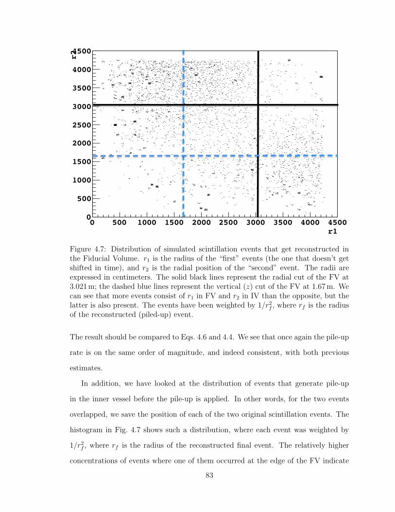
r10 500 1000 1500 2000 2500 3000 3500 4000 4500

r2

0

500

1000

1500

2000

2500

3000

3500

4000

4500r1r2

Figure 4.7: Distribution of simulated scintillation events that get reconstructed inthe Fiducial Volume. r1 is the radius of the “first” events (the one that doesn’t getshifted in time), and r2 is the radial position of the “second” event. The radii areexpressed in centimeters. The solid black lines represent the radial cut of the FV at3.021 m; the dashed blue lines represent the vertical (z) cut of the FV at 1.67 m. Wecan see that more events consist of r1 in FV and r2 in IV than the opposite, but thelatter is also present. The events have been weighted by 1/r2

f , where rf is the radiusof the reconstructed (piled-up) event.

The result should be compared to Eqs. 4.6 and 4.4. We see that once again the pile-up

rate is on the same order of magnitude, and indeed consistent, with both previous

estimates.

In addition, we have looked at the distribution of events that generate pile-up

in the inner vessel before the pile-up is applied. In other words, for the two events

overlapped, we save the position of each of the two original scintillation events. The

histogram in Fig. 4.7 shows such a distribution, where each event was weighted by

1/r2f , where rf is the radius of the reconstructed final event. The relatively higher

concentrations of events where one of them occurred at the edge of the FV indicate

83

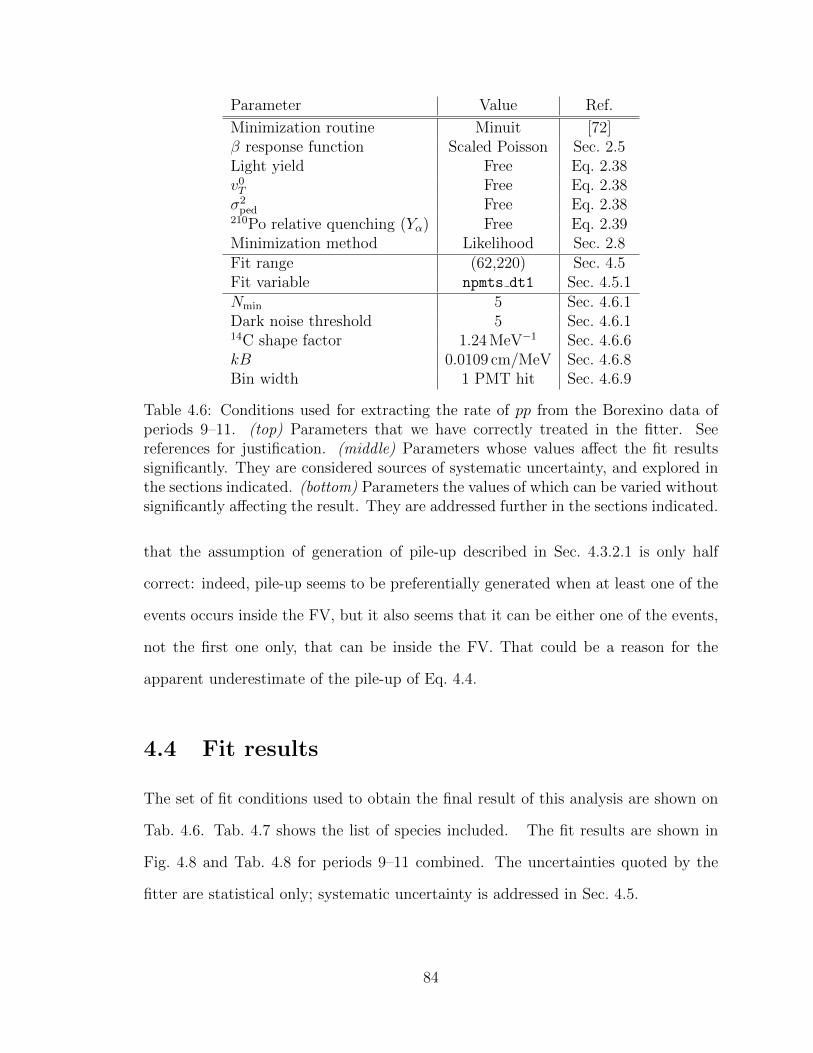
Parameter Value Ref.

Minimization routine Minuit [72]β response function Scaled Poisson Sec. 2.5Light yield Free Eq. 2.38v0T Free Eq. 2.38σ2

ped Free Eq. 2.38210Po relative quenching (Yα) Free Eq. 2.39Minimization method Likelihood Sec. 2.8Fit range (62,220) Sec. 4.5Fit variable npmts dt1 Sec. 4.5.1Nmin 5 Sec. 4.6.1Dark noise threshold 5 Sec. 4.6.114C shape factor 1.24 MeV−1 Sec. 4.6.6kB 0.0109 cm/MeV Sec. 4.6.8Bin width 1 PMT hit Sec. 4.6.9

Table 4.6: Conditions used for extracting the rate of pp from the Borexino data ofperiods 9–11. (top) Parameters that we have correctly treated in the fitter. Seereferences for justification. (middle) Parameters whose values affect the fit resultssignificantly. They are considered sources of systematic uncertainty, and explored inthe sections indicated. (bottom) Parameters the values of which can be varied withoutsignificantly affecting the result. They are addressed further in the sections indicated.

that the assumption of generation of pile-up described in Sec. 4.3.2.1 is only half

correct: indeed, pile-up seems to be preferentially generated when at least one of the

events occurs inside the FV, but it also seems that it can be either one of the events,

not the first one only, that can be inside the FV. That could be a reason for the

apparent underestimate of the pile-up of Eq. 4.4.

4.4 Fit results

The set of fit conditions used to obtain the final result of this analysis are shown on

Tab. 4.6. Tab. 4.7 shows the list of species included. The fit results are shown in

Fig. 4.8 and Tab. 4.8 for periods 9–11 combined. The uncertainties quoted by the

fitter are statistical only; systematic uncertainty is addressed in Sec. 4.5.

84

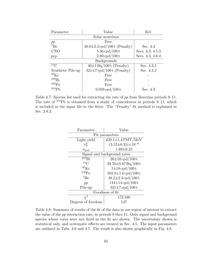
Parameter Value Ref.Solar neutrinos

pp Free -7Be 48.0±2.3 cpd/100 t (Penalty) Sec. 4.3CNO 5.36 cpd/100 t Secs. 4.3, 4.5.3pep 2.80 cpd/100 t Secs. 4.3, 4.6.4

Backgrounds14C 40±1 Bq/100 t (Penalty) Sec. 4.3.1Synthetic Pile-up 321±7 cpd/100 t (Penalty) Sec. 4.3.285Kr Free -210Bi Free -210Po Free -214Pb 0.059 cpd/100 t Sec. 4.3

Table 4.7: Species list used for extracting the rate of pp from Borexino periods 9–11.The rate of 214Pb is obtained from a study of coincidences in periods 9–11, whichis included in the input file to the fitter. The “Penalty” fit method is explained inSec. 2.8.3.

Parameter ValueFit parameters

Light yield 420.1±1.4 PMT/MeVv0T (3.12±0.35)×10−6

σped 1.69±0.23Signal and background rates210Bi 26±10 cpd/100 t14C 39.76±0.87 Bq/100 t

85Kr 1±18 cpd/100 t210Po 582.8±1.6 cpd/100 t7Be 48.2±2.3 cpd/100 tpp 144±14 cpd/100 t

Pile-up 321±7 cpd/100 tGoodness of fit

χ2 172.346Degrees of freedom 147

Table 4.8: Summary of results of the fit of the data in our region of interest to extractthe value of the pp interaction rate, in periods 9 thru 11. Only signal and backgroundspecies whose rates were not fixed in the fit are shown. The uncertainty shown isstatistical only, and systematic effects are treated in Sec. 4.5. The input parametersare outlined in Tabs. 4.6 and 4.7. The result is also shown graphically in Fig. 4.8.

85

1.4 PMT/MeV]±PMTs hit [LY = 420.1 60 80 100 120 140 160 180 200 220 240

Eve

nts

/ (d

ay x

100

to

ns

x 1

PM

T)

-410

-310

-210

-110

1

10

210

310

410

510 Data from 30276.7 days x tons livetime^2/N-DOF = 172.346 / 147χTotal spectrum,

10 cpd/100 tons±Bi = 26 210

0.87 Bq/100 tons [Penalty]±C = 39.76 14

18 cpd/100 tons±Kr = 1 85

Pb = 0.0594 cpd/100 tons [Fixed]214

1.6 cpd/100 tons±Po = 582.8 210

0.096 cpd/100 tons [Penalty]± = 1.976 384

Be)7(ν 2.2 cpd/100 tons [Penalty]± = 46.2

862Be)7(ν

(CNO) = 5.36 cpd/100 tons [Fixed]ν(pep) = 2.8 cpd/100 tons [Fixed]ν

14 cpd/100 tons±(pp) = 144 ν 7 cpd/100 tons [Penalty]±synthpup = 321.1

1.4 PMT/MeV]±PMTs hit [LY = 420.1 80 100 120 140 160 180 200 220

Res

idu

als,

(d

ata

- fi

t) /

sig

ma

-3

-2

-1

0

1

2

3

4

Figure 4.8: (top) Fit of the data in our energy region of interest to extract the valueof the pp interaction rate, in periods 9–11. The results of the fit are also outlinedon Tab. 4.8. The two 7Be neutrinos seen in Fig. 1.3 are shown separately in thelegend here, but their spectral shapes are added together and plotted as one species.(bottom) Residuals of the fit.

86

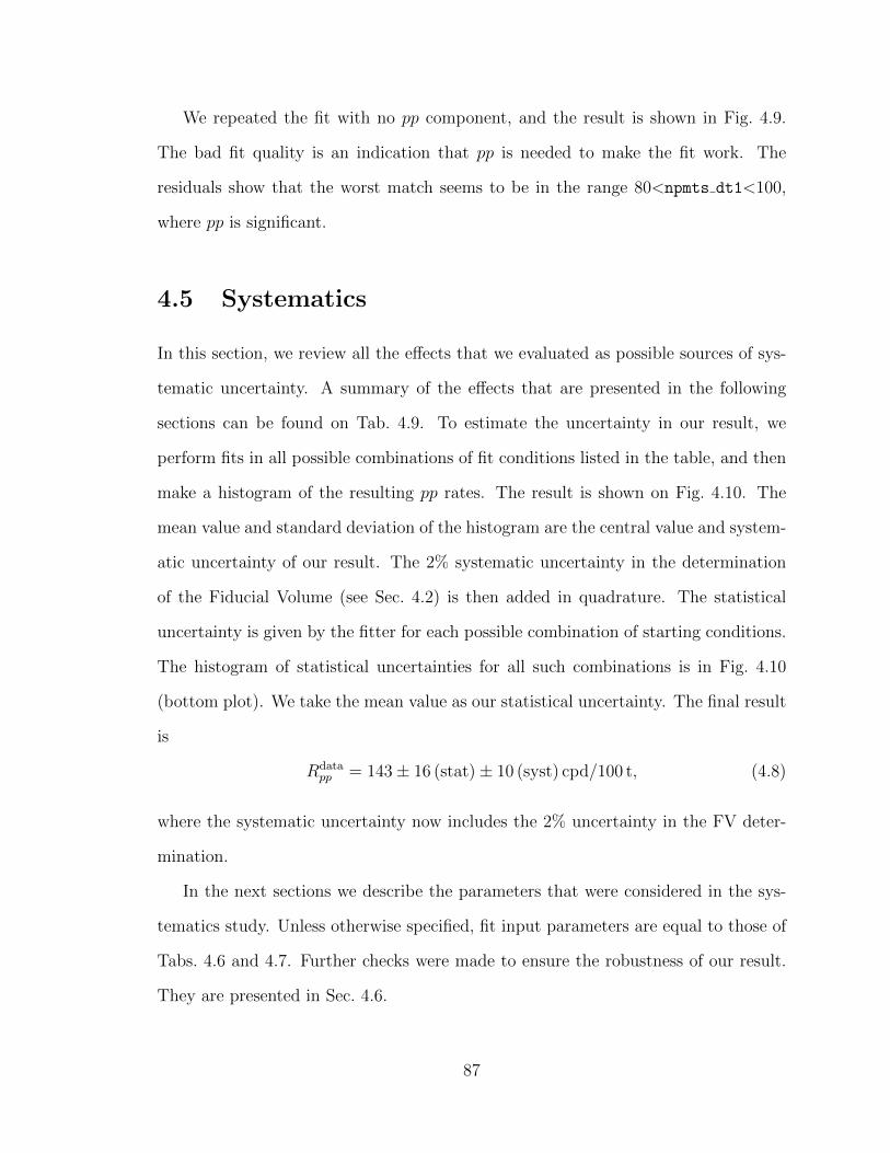
We repeated the fit with no pp component, and the result is shown in Fig. 4.9.

The bad fit quality is an indication that pp is needed to make the fit work. The

residuals show that the worst match seems to be in the range 80<npmts dt1<100,

where pp is significant.

4.5 Systematics

In this section, we review all the effects that we evaluated as possible sources of sys-

tematic uncertainty. A summary of the effects that are presented in the following

sections can be found on Tab. 4.9. To estimate the uncertainty in our result, we

perform fits in all possible combinations of fit conditions listed in the table, and then

make a histogram of the resulting pp rates. The result is shown on Fig. 4.10. The

mean value and standard deviation of the histogram are the central value and system-

atic uncertainty of our result. The 2% systematic uncertainty in the determination

of the Fiducial Volume (see Sec. 4.2) is then added in quadrature. The statistical

uncertainty is given by the fitter for each possible combination of starting conditions.

The histogram of statistical uncertainties for all such combinations is in Fig. 4.10

(bottom plot). We take the mean value as our statistical uncertainty. The final result

is

Rdatapp = 143± 16 (stat)± 10 (syst) cpd/100 t, (4.8)

where the systematic uncertainty now includes the 2% uncertainty in the FV deter-

mination.

In the next sections we describe the parameters that were considered in the sys-

tematics study. Unless otherwise specified, fit input parameters are equal to those of

Tabs. 4.6 and 4.7. Further checks were made to ensure the robustness of our result.

They are presented in Sec. 4.6.

87

1.4 PMT/MeV]±PMTs hit [LY = 420.1 60 80 100 120 140 160 180 200 220 240

Eve

nts

/ (d

ay x

100

to

ns

x 1

PM

T)

-310

-210

-110

1

10

210

310

410

510 Data from 30276.7 days x tons livetime^2/N-DOF = 276.289 / 148χTotal spectrum,

8.4 cpd/100 tons±Bi = 9 210

0.83 Bq/100 tons [Penalty]±C = 42.21 14

6.5 cpd/100 tons±Kr = 30.8 85

Pb = 0.0594 cpd/100 tons [Fixed]214

1.5 cpd/100 tons±Po = 578.2 210

0.094 cpd/100 tons [Penalty]± = 1.921 384

Be)7(ν

2.2 cpd/100 tons [Penalty]± = 44.9 862

Be)7(ν(CNO) = 5.36 cpd/100 tons [Fixed]ν(pep) = 2.8 cpd/100 tons [Fixed]ν

7 cpd/100 tons [Penalty]±synthpup = 324.9

1.2 PMT/MeV]±PMTs hit [LY = 415.4 80 100 120 140 160 180 200 220

Res

idu

als,

(d

ata

- fi

t) /

sig

ma

-4

-3

-2

-1

0

1

2

3

4

Figure 4.9: (top) Fit of the data in our energy region of interest against all thebackgrounds to the pp neutrino signal, without including pp as a species. The bad fitquality is an indication that pp is needed to make the fit work. The valley between 14Cand 210Po shows bad match between data and analytical spectra. (bottom) Residualsof the fit, showing worst match in a region where pp is significant.

88

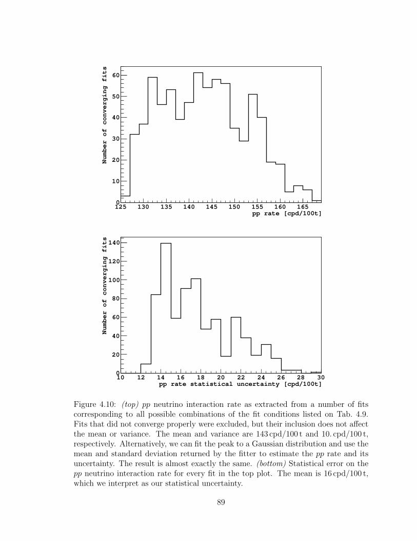
pp rate [cpd/100t]125 130 135 140 145 150 155 160 165

Number of converging fits

0

10

20

30

40

50

60

pp rate statistical uncertainty [cpd/100t]10 12 14 16 18 20 22 24 26 28 30

Number of converging fits

0

20

40

60

80

100

120

140

Figure 4.10: (top) pp neutrino interaction rate as extracted from a number of fitscorresponding to all possible combinations of the fit conditions listed on Tab. 4.9.Fits that did not converge properly were excluded, but their inclusion does not affectthe mean or variance. The mean and variance are 143 cpd/100 t and 10. cpd/100 t,respectively. Alternatively, we can fit the peak to a Gaussian distribution and use themean and standard deviation returned by the fitter to estimate the pp rate and itsuncertainty. The result is almost exactly the same. (bottom) Statistical error on thepp neutrino interaction rate for every fit in the top plot. The mean is 16 cpd/100 t,which we interpret as our statistical uncertainty.

89

Source Values Sec.

Pile-up method Synthetic,Convolution 4.5.1Choice of variable npmts dt1,npmts dt2 4.5.1

Choice of FV 0,2,3,4 4.5.2Rate of CNO 5.4±2.5 cpd/100 t 4.5.3Fit start point 56,60,65,70 -Fit end point 215,220,225 -

FV determination 2% 4.2

Statistics 11% 4.4

Table 4.9: List of systematic effects considered in the fit. “Choice of FV” refersto a freedom of choice of the FV used for the analysis, while “FV determination”refers to the uncertainty in the shape of the FV coming from the uncertainty of theposition reconstruction algorithm. For every combination of pile-up method, fiducialvolume, variable and fit range, five random values of the CNO rate are drawn froma Gaussian distribution with the mean and standard deviation indicated. The totalsystematic uncertainty (excluding the FV determination) is obtained by making ahistogram of the pp rate obtained by all resulting combinations of fit conditions. TheFV determination uncertainty and the statistic uncertainty are added in quadrature atthe end. The statistical uncertainty is equal to the mean of the statistical uncertaintiescoming out of these fits (see text).

npmts dt1 npmts dt2

Synthetic pile-up 154±13 150±13Convolution method 154±13 164±13

Table 4.10: Results of fits in all combinations of pile-up method (synthetic pile-upand convolution method) and fit variable (npmts dt1 and npmts dt2). As the datasets are essentially the same, the variations in the central value are an indication ofsystematic uncertainty.

4.5.1 Pile-up estimation method and fit variable

In Sec. 4.3.2 we talked about various ways in which we could estimate pile-up. We

believe that the two most reliable methods are the synthetic (Sec. 4.3.2.1) and con-

volution (Sec. 4.3.2.2) methods. Previously, in Sec. 2.4, we had talked about two

energy estimators, npmts dt1 and npmts dt2, and said we would perform the fit in

npmts dt1, but should check the results using npmts dt2.

We performed fits with all combinations of pile-up method and fit variable. The

results are shown on Tab. 4.10. As the data sets are essentially the same, the variations

90

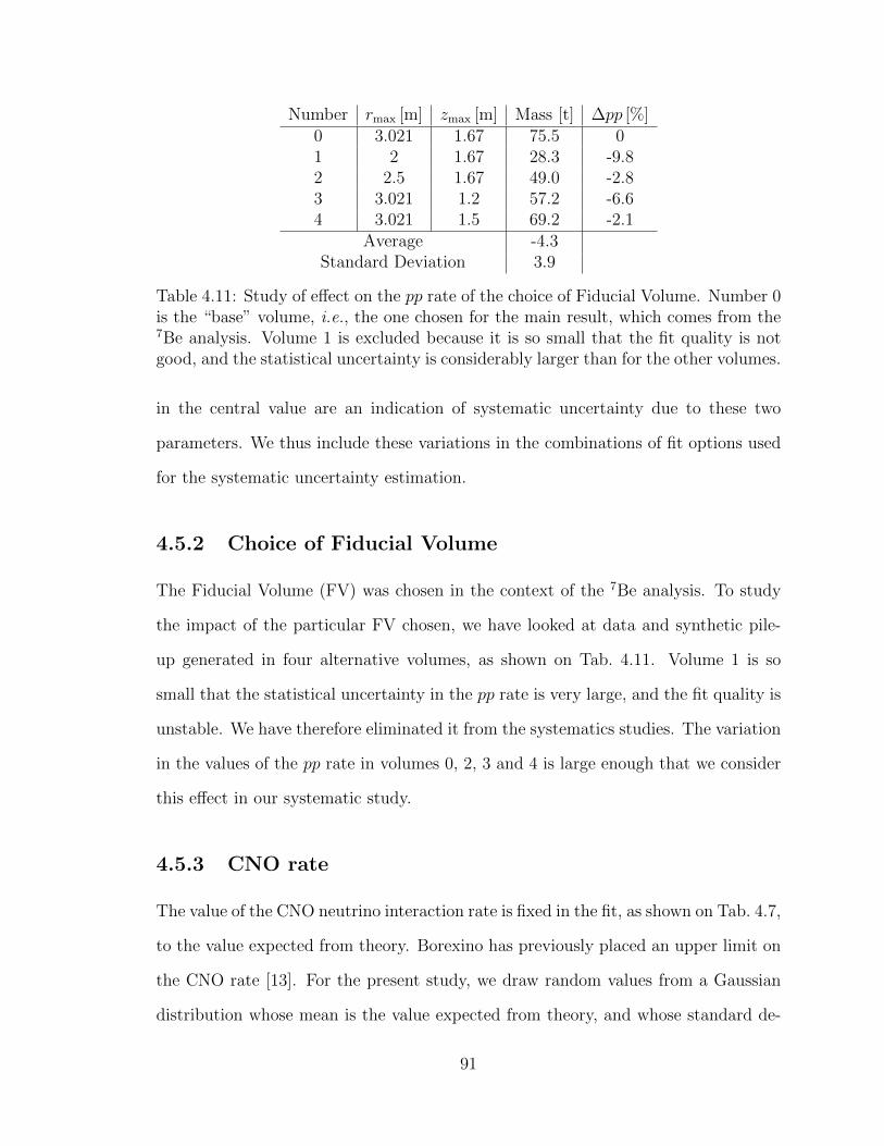
Number rmax [m] zmax [m] Mass [t] ∆pp [%]0 3.021 1.67 75.5 01 2 1.67 28.3 -9.82 2.5 1.67 49.0 -2.83 3.021 1.2 57.2 -6.64 3.021 1.5 69.2 -2.1

Average -4.3Standard Deviation 3.9

Table 4.11: Study of effect on the pp rate of the choice of Fiducial Volume. Number 0is the “base” volume, i.e., the one chosen for the main result, which comes from the7Be analysis. Volume 1 is excluded because it is so small that the fit quality is notgood, and the statistical uncertainty is considerably larger than for the other volumes.

in the central value are an indication of systematic uncertainty due to these two

parameters. We thus include these variations in the combinations of fit options used

for the systematic uncertainty estimation.

4.5.2 Choice of Fiducial Volume

The Fiducial Volume (FV) was chosen in the context of the 7Be analysis. To study

the impact of the particular FV chosen, we have looked at data and synthetic pile-

up generated in four alternative volumes, as shown on Tab. 4.11. Volume 1 is so

small that the statistical uncertainty in the pp rate is very large, and the fit quality is

unstable. We have therefore eliminated it from the systematics studies. The variation

in the values of the pp rate in volumes 0, 2, 3 and 4 is large enough that we consider

this effect in our systematic study.

4.5.3 CNO rate

The value of the CNO neutrino interaction rate is fixed in the fit, as shown on Tab. 4.7,

to the value expected from theory. Borexino has previously placed an upper limit on

the CNO rate [13]. For the present study, we draw random values from a Gaussian

distribution whose mean is the value expected from theory, and whose standard de-

91

viation is the difference between that value and the upper limit placed by Borexino.

We draw five values for each combination of all the other effects under consideration.

4.6 Checks

In this section we elaborate on several checks performed to look for other systematic

effects.

4.6.1 Choice of Nmin

As explained in Sec. 4.3.2.1, the creation of the synthetic pile-up spectrum depends

on a parameter called Nmin, which represents the minimum increase in the npmts dt1

or npmts dt2 variable that is required to define a synthetic event as a pile-up event.

At the same time, the summation in Eq. 2.56 over the number of dark noise hits

is truncated at some value of npmts win1, above which signal and background events

are included, not just dark noise. We chose a dark noise threshold equal to Nmin. A

number of hits larger than Nmin is assumed to come from a scintillation event, not

dark noise, and thus it is included as pile-up.

We chose Nmin = 5, but this choice was not exclusive. We tried Nmin = 3, 7 and

10, and found consistent results in all cases.

4.6.2 Synthetic pile-up statistics

In Sec. 4.3.2.1 we generated synthetic pile-up for an exposure corresponding to four

times the exposure of the regular data. To check that this is sufficient statistics,

we have used simulator (Sec. 2.8.1) to draw random “events” from the analytical

14C pile-up distribution to match the statistics of the synthetic pile-up, four times.

We thus obtain four histograms, each with a simulated live time equal to four times

the exposure of the real data sample. In all cases, we input the resulting histogram

92

as a simulated synthetic pile-up spectrum into the fit as in Sec. 4.4, with its rate

constrained by the generated number of events, and obtain results consistent with

each other.

4.6.3 14C rate estimate

In Sec. 4.3.1 we estimated the 14C rate by looking at second clusters. We then

used that rate in the fit of Sec. 4.4, to constrain the possible values of the 14C rate

with a penalty factor. The constraint can be relaxed if we choose to start the fit

at npmts dt1=60, so that a larger portion of the 14C spectrum is included in the

fit. When we do this, we obtain a value for the pp rate consistent with our final

result (Eq. 4.8), and a 14C rate of 40.0±0.7 cpd/100 t, in perfect agreement with the

independent estimate.

4.6.4 pep rate

The pep rate was fixed in the fitter to the value expected from theory. We have tried

alternative values within the 1σ range provided by the Borexino measurement [13].

No variations in the pp rate were observed.

4.6.5 Soft α/β cut

This cut, as explained in Sec. 4.2, can cause trouble because it deforms the synthetic

pile-up in ways that we cannot exactly model currently. For this reason, it has not

been employed in the main data set. However, data and synthetic pile-up spectra

have also been produced, in parallel to the main analysis, with this cut in place. The

effect of the cut on these can be seen in Fig. 4.11. With these files as inputs, the pp

rate has been extracted in the same way as in Sec. 4.4. The result is consistent.

93

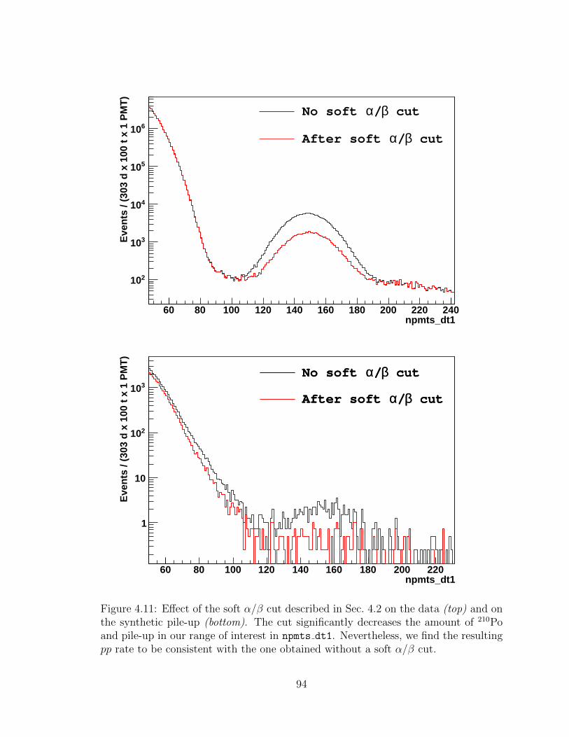
npmts_dt160 80 100 120 140 160 180 200 220 240

Eve

nts

/ (3

03 d

x 1

00 t

x 1

PM

T)

210

310

410

510

610

cutβ/αNo soft

cutβ/αAfter soft

npmts_dt160 80 100 120 140 160 180 200 220

Eve

nts

/ (3

03 d

x 1

00 t

x 1

PM

T)

1

10

210

310

cutβ/αNo soft

cutβ/αAfter soft

cutβ/αNo soft

cutβ/αAfter soft

Figure 4.11: Effect of the soft α/β cut described in Sec. 4.2 on the data (top) and onthe synthetic pile-up (bottom). The cut significantly decreases the amount of 210Poand pile-up in our range of interest in npmts dt1. Nevertheless, we find the resultingpp rate to be consistent with the one obtained without a soft α/β cut.

94

4.6.6 14C shape factor

As explained in Sec. 2.7.2.1 and Tab. 4.6, we assumed a 14C spectral shape factor of

1.24 MeV−1 [58]. To test our sensitivity to this choice, we have repeated the fit with

the other two values shown in Tab. 2.3. The effect on the pp rate of this variation is

negligible.

4.6.7 210Bi spectral shape

The 210Bi spectral shape included in spectral-fitter was obtained in the context

of the 7Be analysis [64, 36]. Updates by the CNO working group have found two

other shape factor functions [73, 74] that could alter the spectral shape considerably.

We show the absolute and relative shapes in Fig. 4.12. By replacing the current 210Bi

spectrum in spectral-fitter by the two shapes mentioned above, we can estimate

the effect on the pp rate at <1%.

4.6.8 kB

The value of Birks’ constant kB, a scintillator property, is known to be∼0.01 cm/MeV

from previous studies [36]. The exact number is still somewhat uncertain, and we

chose to work with kB=0.0109 cm/MeV because it was the value obtained in the

7Be analysis. We know, however, that some Monte Carlo work showed evidence of

kB = 0.0104 cm/MeV (see Chapter 3). We have thus re-done the fit of Sec. 4.4 with

kB = 0.0105 cm/MeV and kB = 0.0115 cm/MeV. No change in the resulting pp rate

was observed.

4.6.9 Histogram binning

The histograms were all binned in intervals of 1 PMT, as at these low energies a

difference of 1 in npmts dt1 is rather significant. To ensure that we are not overly

95

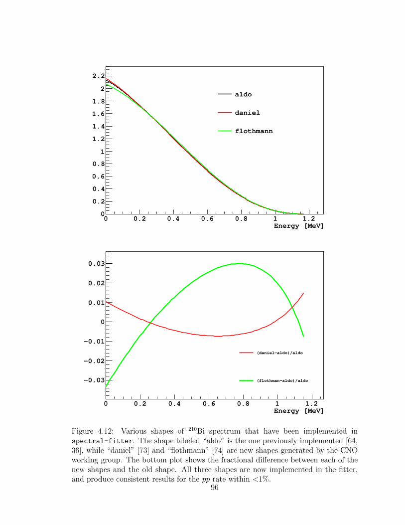
Energy [MeV]0 0.2 0.4 0.6 0.8 1 1.20

0.2

0.4

0.6

0.8

1

1.2

1.4

1.6

1.8

2

2.2

aldo

daniel

flothmann

Energy [MeV]0 0.2 0.4 0.6 0.8 1 1.2

-0.03

-0.02

-0.01

0

0.01

0.02

0.03

(daniel-aldo)/aldo

(flothman-aldo)/aldo

Figure 4.12: Various shapes of 210Bi spectrum that have been implemented inspectral-fitter. The shape labeled “aldo” is the one previously implemented [64,36], while “daniel” [73] and “flothmann” [74] are new shapes generated by the CNOworking group. The bottom plot shows the fractional difference between each of thenew shapes and the old shape. All three shapes are now implemented in the fitter,and produce consistent results for the pp rate within <1%.

96

sensitive to the variations between bins, we have re-done the fit with a binning of 2,

and the variations were <1%, which we can neglect.

4.6.10 87Rb rate

In Sec. 2.7.2.4 we concluded that 87Rb was a negligible source of background

(<0.1 cpd/100 t) if we assumed that the relative proportions of 87Rb and 40K in our

scintillator were the same as in average Earth crust materials. A recent measurement

of purified sodium iodide for crystal growth has seen 87Rb enriched by a factor of

200. This, however, was a different purification method specifically designed for

the removal of 40K, and in solid state. Nevertheless, if we assume this pessimistic

enrichment, we can limit the 87Rb rate to <20 cpd/100 t.

We re-did the fit of Fig. 4.8, with the added component of 87Rb, varying its rate

between 0 and 20 cpd/100 t. The effect on the pp rate is shown in Fig. 4.13. By fitting

the data to a straight line, we find a slope of -0.38. That means that an increase of

the 87Rb rate of 1 cpd/100 t induces a decrease in the pp rate of 0.38 cpd/100 t. Thus,

the uncertainty in the pp rate induced by 87Rb, assuming the enhanced amount of

87Rb, is <8 cpd/100 t, which is 6% of the measured pp rate. Once again, though, since

we believe there is no reason to assume this level of enrichment, we neglect 87Rb.

4.6.11 Choice of period

As explained in Sec. 4.1, the data set was chosen to maximize the statistics. However,

we would like to ensure that the same analysis run on sub-periods produces consistent

results. We have analyzed periods 9, 10 and 11 individually, as well as 10–11 combined

and 9–12 combined. The results were all consistent within one statistical standard

deviation. This check also ensures that we are not sensitive to the change in the BTB

threshold that occurred during period 11.

97

Rb rate [cpd/100 t]870 5 10 15 20

pp rate [cpd/100 t]

110

120

130

140

150

160

170Rb87Profile of pp versus

Figure 4.13: Rate of pp versus rate of 87Rb as obtained from including 87Rb as aspecies in the fit of Fig. 4.8, with its rate fixed at various values between 0 and20 cpd/100 t. A fit to a straight line returns a slope of -0.38, meaning that the pp ratedecreases by ∼0.4 cpd/100 t for every cpd/100 t of 87Rb.

98

4.6.12 Penalty factor for pile-up

The rate of synthetic pile-up is constrained in the fit by applying a penalty factor,

whose central value is the integral of the synthetic pile-up spectrum, divided by

its corresponding exposure. To account for possible unknown systematics, we have

enlarged the standard deviation for the penalty factor to 10% of the synthetic pile-up

rate. The resulting rate of pp was not altered at all. We conclude that this does not

affect the analysis, as there is no reason to believe the uncertainty in the synthetic

pile-up rate should be enlarged.

4.6.13 Threshold for photoelectron detection

In all of our previous derivations we have assumed that any PMT hit by a photon

that converts to a photoelectron will be considered triggered. This is not the case in

reality, for a PMT is considered triggered only if the integrated charge exceeds some

threshold (Sec. 2.3). This means that PMTs recording multiple photoelectrons are

more likely to trigger than PMTs registering a single photoelectron. Here we estimate

the effect by looking at the probability that a PMT registers more than one hit. The

threshold effect on single-hit PMTs will be absorbed by the light yield, which is a

free parameter of the fit.

Suppose we observe a scintillation event of Np photoelectrons that took place at

radius r. We can make the rough assumption that only the PMT closest to the event

can register multiple hits. The mean area per PMT 11 in Borexino is simply given by

A1 =4πR2

NT

(4.9)

11This is not the surface area of a PMT, but the surface area of the SSS, divided by the numberof PMTs. Since the reflectivity of the walls is lower than 100%, the effective mean area per PMTshould, in reality, be smaller than the number assumed here.

99

where R is the radius of the Stainless Steel Sphere (6.85 m), and NT is the total

number of PMTs installed (∼2200). For an event at radius r, the solid angle occupied

by the closest PMT is approximately

Ω1(r) =4πR2/NT

4π(R− r)24π =

4π

NT (1− r/R)2(4.10)

The mean number of photoelectrons in that PMT, then, is

Np1(r) =NpΩ1(r)

4π=

Np

NT (1− r/R)2(4.11)

We would like to average this over the entire Fiducial Volume

〈Np1(r)〉 =1

VFV

∫FV

Np

NT (1− r/R)2d3r (4.12)

Then we want to average over all Np in our energy range of interest

〈Np1(r)〉 =

∑Npmax

Npmin

1VFV

∫FV

NpNT (1−r/R)2

d3r × q(Np)∑Npmax

Npminq(Np)

(4.13)

where q(Np) is the data spectrum. If we assume conservatively that the Fiducial

Volume is a sphere of radius RFV = 3 m (the real Fiducial Volume, defined in Sec. 4.2,

is approximately a subset of this one), we get

〈Np1(r)〉 =3R3

R3FV

[RFV

R

(2−RFV/R

1−RFV/R

)+ 2 ln

(1− RFV

R

)]1

NT

Np (4.14)

where Np is the mean of Np in our data spectrum. In periods 9–11 combined, Np = 69.

Plugging all the values in, we get

〈Np1(r)〉 = 0.09 (4.15)

100

This means that the mean number of photoelectrons in the nearest PMT for an aver-

age scintillation event in our FV is 0.09. Assuming Poisson statistics, the probability

that more than one photoelectron is detected by a PMT is then

P>1 = 1− (1 + 0.09)e−0.09 = 0.004 (4.16)

This means that 0.4% of events were affected by this effect, so we can neglect it.

101

Chapter 5

Interpretation of results

A correct estimation of the pp neutrino interaction rate in Borexino requires an un-

derstanding of three key physics elements: nuclear physics, particle physics and as-

trophysics. The nuclear physics comes into play in the Sun, where nuclear processes

give rise to the generation of energy in the form of photons, neutrinos and other par-

ticles. Particle physics dictates the way in which neutrinos move through the Sun,

then through space, and then through our atmosphere and Earth, to finally arrive at

Borexino and interact with electrons in the scintillator. Finally, it is impossible to

develop a solar model without an understanding of the astrophysics of the Sun: this

brings in quantum mechanics, thermodynamics and nuclear physics to explain how

a massive object can form the way it does. In particular, the Standard Solar Model

is developed under the assumption that the neutrino luminosity coming out of the

Sun can be related to the photon luminosity. This is equivalent to assuming that the

core of the Sun has not evolved significantly in the past ten million years, the time it

takes for photons to travel from the core of the Sun to its surface.

After years of developing theories that allow for the creation of the Standard

Solar Model, we have finally arrived at a point where we can verify our hypotheses,

and measurements like the pep and 7Be interaction rates in Borexino confirm our

102

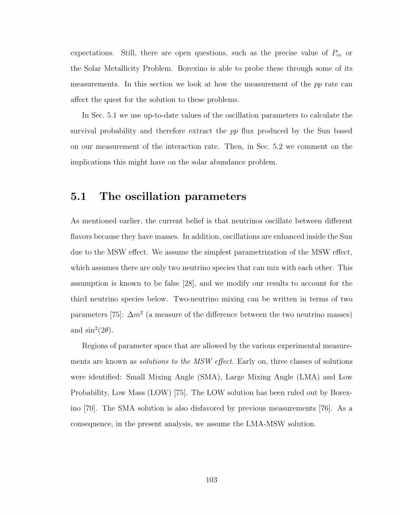
expectations. Still, there are open questions, such as the precise value of Pee or

the Solar Metallicity Problem. Borexino is able to probe these through some of its

measurements. In this section we look at how the measurement of the pp rate can

affect the quest for the solution to these problems.

In Sec. 5.1 we use up-to-date values of the oscillation parameters to calculate the

survival probability and therefore extract the pp flux produced by the Sun based

on our measurement of the interaction rate. Then, in Sec. 5.2 we comment on the

implications this might have on the solar abundance problem.

5.1 The oscillation parameters

As mentioned earlier, the current belief is that neutrinos oscillate between different

flavors because they have masses. In addition, oscillations are enhanced inside the Sun

due to the MSW effect. We assume the simplest parametrization of the MSW effect,

which assumes there are only two neutrino species that can mix with each other. This

assumption is known to be false [28], and we modify our results to account for the

third neutrino species below. Two-neutrino mixing can be written in terms of two

parameters [75]: ∆m2 (a measure of the difference between the two neutrino masses)

and sin2(2θ).

Regions of parameter space that are allowed by the various experimental measure-

ments are known as solutions to the MSW effect. Early on, three classes of solutions

were identified: Small Mixing Angle (SMA), Large Mixing Angle (LMA) and Low

Probability, Low Mass (LOW) [75]. The LOW solution has been ruled out by Borex-

ino [70]. The SMA solution is also disfavored by previous measurements [76]. As a

consequence, in the present analysis, we assume the LMA-MSW solution.

103

From [6] we know that the 2-neutrino approximation can be obtained by assuming

sin2 2θ = sin2 2θ12 and ∆m2 = ∆m221. We use the Normal Hierarchy values from [77] 1:

sin2 θ12 = 0.307± 0.018

∆m221 = (7.54± 0.26) · 10−5 eV2 (5.1)

sin2 θ13 = 0.0241± 0.0025

The value of θ13 will be used later. In addition, we know from [56] that the electron-

neutrino survival probability at pp energies can be written as

P 2νee (Eν) =

1

2+

1

2(1− δpp) cos 2θm(V pp) cos 2θ (5.2)

where

δpp =3

2

(2EνV pp/∆m2)2 sin2 2θ

[(cos 2θ − 2EνV pp/∆m2)2 + sin2 2θ]2∆V 2

pp

V2

pp

(5.3)

cos 2θm(V ) =cos 2θ − 2EνV/∆m

2

[(cos 2θ − 2EνV/∆m2)2 + sin2 2θ]1/2(5.4)

V pp = 4.68 · 10−12 eV (5.5)

∆V 2pp = V

2

pp · 0.109 (5.6)

cos 2θ =√

1− sin2 2θ (5.7)

and Eν is the neutrino energy. θm is the mixing angle in matter; it is a function of the

interaction potential V , which in turn is a function of the electron density in the core

of the Sun. Because the sources of the various neutrino species are not distributed

equally in the core of the Sun, the potential is different for different neutrino species.

It is possible to approximate the potential by its mean and variance (V pp and ∆V 2pp,

respectively, for pp neutrinos).

1The effect of the Inverted Hierarchy would be exceedingly small and can be neglected.

104

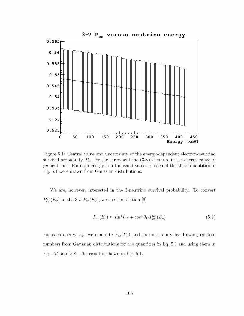
Energy [keV]0 50 100 150 200 250 300 350 400 450

0.525

0.53

0.535

0.54

0.545

0.55

0.555

0.56

0.565

versus neutrino energyee Pν3-

Figure 5.1: Central value and uncertainty of the energy-dependent electron-neutrinosurvival probability, Pee, for the three-neutrino (3-ν) scenario, in the energy range ofpp neutrinos. For each energy, ten thousand values of each of the three quantities inEq. 5.1 were drawn from Gaussian distributions.

We are, however, interested in the 3-neutrino survival probability. To convert

P 2νee (Eν) to the 3-ν Pee(Eν), we use the relation [6]

Pee(Eν) ≈ sin4 θ13 + cos4 θ13P2νee (Eν) (5.8)

For each energy Eν , we compute Pee(Eν) and its uncertainty by drawing random

numbers from Gaussian distributions for the quantities in Eq. 5.1 and using them in

Eqs. 5.2 and 5.8. The result is shown in Fig. 5.1.

105

Now we return to Eq. 2.41, noting that the total detection rate R is the integral

of the detection spectrum:

Rpp =

∫ ∞0

hpp(E) dE =

∫ ∞0

φ

∫ Emaxν

0

[S(Eν) dEν ]×(n

dσ

dE(Eν , E) dE

)(5.9)

where n is the electron density. Plugging in Eq. 2.43, we obtain

Rpp = φn

∫ ∞0

∫ Emaxν

0

S(Eν)

[Pee(Eν)

dσedE

(Eν , E) + [1− Pee(Eν)]dσµ,τdE

(Eν , E)

]dEν dE

(5.10)

Note that, for a specific neutrino energy, the maximum recoil energy is defined by

kinematics as in Eq. 2.42. With that in mind, we can invert the order of the integrals

Rpp = φn

∫ Emaxν

0

∫ Emax(Eν)

0

S(Eν)

[Pee(Eν)

dσedE

(Eν , E) + [1− Pee(Eν)]dσµ,τdE

(Eν , E)

]dE dEν

(5.11)

Now we can perform the integral over the recoil energy E

Rpp = φn

∫ Emaxν

0

S(Eν) Pee(Eν)σe(Eν) + [1− Pee(Eν)]σµ,τ (Eν) dEν (5.12)

σi(Eν) ≡∫ Emax(Eν)

0

dσidE

(Eν , E) dE; i = e, µ, τ (5.13)

Noting from Fig. 5.1 that the variation of Pee(E) within the energy range of pp

neutrinos is smaller than its uncertainty, we replace the energy-dependent Pee(E) by

106

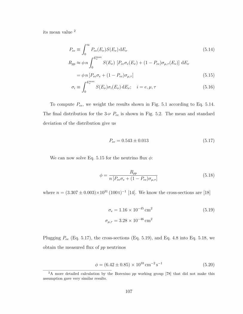
its mean value 2

Pee ≡∫ ∞

0

Pee(Eν)S(Eν) dEν (5.14)

Rpp ≈ φn

∫ Emaxν

0

S(Eν) [Peeσe(Eν) + (1− Pee)σµ,τ (Eν)] dEν

= φn [Peeσe + (1− Pee)σµ,τ ] (5.15)

σi ≡∫ Emax

ν

0

S(Eν)σi(Eν) dEν ; i = e, µ, τ (5.16)

To compute Pee, we weight the results shown in Fig. 5.1 according to Eq. 5.14.

The final distribution for the 3-ν Pee is shown in Fig. 5.2. The mean and standard

deviation of the distribution give us

Pee = 0.543± 0.013 (5.17)

We can now solve Eq. 5.15 for the neutrino flux φ:

φ =Rpp

n [Peeσe + (1− Pee)σµ,τ ](5.18)

where n = (3.307± 0.003)×1031 (100 t)−1 [14]. We know the cross-sections are [18]

σe = 1.16× 10−45 cm2 (5.19)

σµ,τ = 3.28× 10−46 cm2

Plugging Pee (Eq. 5.17), the cross-sections (Eq. 5.19), and Eq. 4.8 into Eq. 5.18, we

obtain the measured flux of pp neutrinos

φ = (6.42± 0.85)× 1010 cm−2 s−1 (5.20)

2A more detailed calculation by the Borexino pp working group [78] that did not make thisassumption gave very similar results.

107

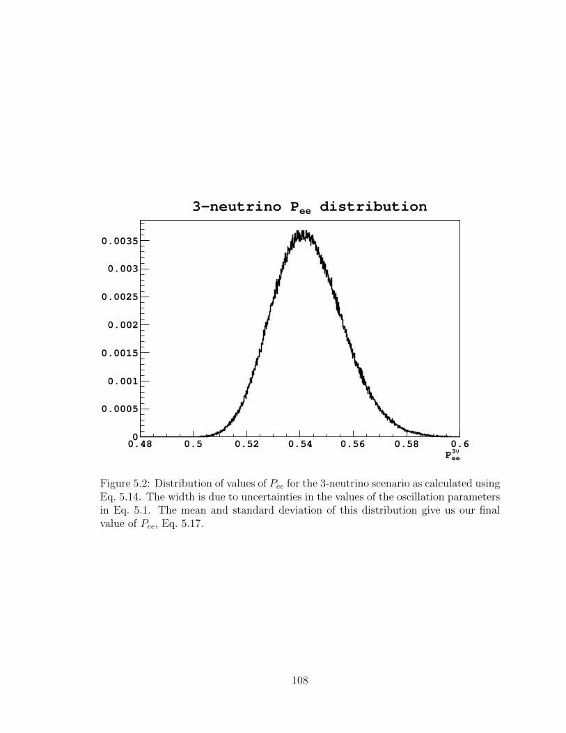
ν3eeP

0.48 0.5 0.52 0.54 0.56 0.58 0.60

0.0005

0.001

0.0015

0.002

0.0025

0.003

0.0035

distributionee3-neutrino P

Figure 5.2: Distribution of values of Pee for the 3-neutrino scenario as calculated usingEq. 5.14. The width is due to uncertainties in the values of the oscillation parametersin Eq. 5.1. The mean and standard deviation of this distribution give us our finalvalue of Pee, Eq. 5.17.

108

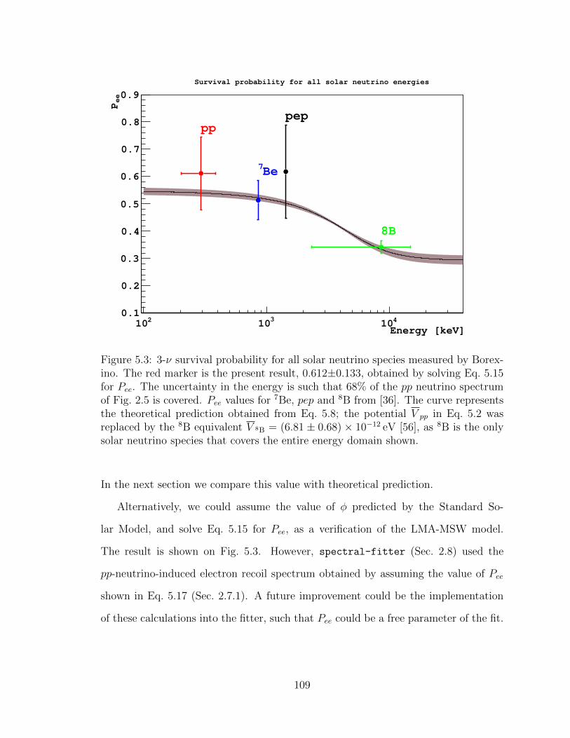
Energy [keV]210 310 410

ee

P

0.1

0.2

0.3

0.4

0.5

0.6

0.7

0.8

0.9

pp

Be7

pep

8B

Survival probability for all solar neutrino energies

Figure 5.3: 3-ν survival probability for all solar neutrino species measured by Borex-ino. The red marker is the present result, 0.612±0.133, obtained by solving Eq. 5.15for Pee. The uncertainty in the energy is such that 68% of the pp neutrino spectrumof Fig. 2.5 is covered. Pee values for 7Be, pep and 8B from [36]. The curve representsthe theoretical prediction obtained from Eq. 5.8; the potential V pp in Eq. 5.2 wasreplaced by the 8B equivalent V 8B = (6.81 ± 0.68) × 10−12 eV [56], as 8B is the onlysolar neutrino species that covers the entire energy domain shown.

In the next section we compare this value with theoretical prediction.

Alternatively, we could assume the value of φ predicted by the Standard So-

lar Model, and solve Eq. 5.15 for Pee, as a verification of the LMA-MSW model.

The result is shown on Fig. 5.3. However, spectral-fitter (Sec. 2.8) used the

pp-neutrino-induced electron recoil spectrum obtained by assuming the value of Pee

shown in Eq. 5.17 (Sec. 2.7.1). A future improvement could be the implementation

of these calculations into the fitter, such that Pee could be a free parameter of the fit.

109

5.2 The solar abundance problem

We have already seen how the old solar neutrino problem has been solved by the

MSW effect (Sec. 1.3). That did not, however, fully resolve the understanding of solar

physics. In particular, disagreement about the ratio of heavy elements to hydrogen

in the the surface of the sun, (Z/X)S, is known as the solar abundance problem

or solar metallicity problem [17]. The latter term is due to a convention among

astrophysicists that all elements heavier than He are referred to as metals. From [17]

we know the expected pp fluxes of the high- and low-metallicity models are (5.98 ±

0.04)× 1010 cm−2s−1 and (6.03± 0.04)× 1010 cm−2s−1, respectively.

As we can see in Eq. 5.20, our measured flux is consistent with both of these rates 3,

and thus we cannot make a claim about the solar abundance problem. This task will

be tackled by future Borexino measurements, such as that of CNO neutrinos [13], for

which Borexino previously only placed an upper limit.

Note also that due to the small difference between the high- and low-metallicity

predictions of the pp flux, in order to use a measurement of the pp detection rate

to determine which model is more accurate, we would have to achieve a precision

of better than 1%. This would require taking data for many more years, more than

Borexino can continue functioning due to the continual loss of PMTs. Alternatively,

we could work to reduce the pile-up to the point where pp is the main contribu-

tion in the valley between 14C and 210Po. With a 14C rate of ∼40 /s/100 t, and a

scintillator time constant on the order of 100 ns [36], the only hope is to separate

pile-up events from other signal and background events by their different hit time

profiles (Sec. 2.7.2.2). To tune this cut reliably, considerable work is needed on the

simulations front to reproduce data very accurately at low energies.

3As explained in the footnote in the introduction to Chapter 5, the fact that the present mea-surement is consistent with expectation justifies the assumption made by the Standard Solar Modelthat the solar core has been stable for the past ten million years. A previous hypothesis that changesin the solar core over the past four million years were responsible for the terrestrial glacial epochs isthus invalidated [79].

110

Chapter 6

Neutron detection in Borexino

So far we have been discussing the detection of neutrinos in Borexino, which is the

purpose for which the detector was designed. It was noticed early on, however, that

Borexino is also a powerful tool for detecting neutrons.

Neutrons are an irreducible source of background in direct dark matter detection

experiments, for their signatures cannot be distinguished from those of WIMPs [45].

Because of its location next to various dark matter detection experiments, and its em-

ployment of liquid scintillator as a detector material, Borexino is an ideal experiment

for the validation of simulation codes used for dark matter detector design.

The Borexino collaboration released three articles describing cosmogenic muon

and neutron detection [41, 80, 44]. We focus here on the measurements of neutron

rate and multiplicity performed with the PAS (see Sec. 2.3.1), which is an integral

part of [44].

In Sec. 6.1 we describe the hardware and software used for this analysis. Then we

talk about our data and selection in Sec. 6.2, resulting in raw neutron and muon detec-

tion rates. In Sec. 6.3 we outline the corrections for inefficiencies and over-efficiencies

that need to be applied to those rates. Results and conclusions are presented in

Sec. 6.4.

111

6.1 Hardware and Software

The PAS is a single-channel Acquiris DP235 digitizer. The board triggers on the

MTF (see Sec. 2.3) and its input is the analog sum of all 2212 ID PMTs. When the

trigger occurs, data is collected for 1.6 ms. A coarse online cut removes all triggers

that do not have any activity over a baseline. Afterwards, an offline cut finds peaks

that are identified as neutrons, and the data is saved as a ROOT file with a TTree [81]

whose entries are neutrons with the time of arrival after the muon, and the time when

the muon occurred, as well as pulse height and integral information. We later cut on

the amplitude of the pulses as a way to efficiently select neutrons. The amplitude cut

can be translated into a neutron energy, which we describe below.

6.2 Data selection

Data used for the present analysis were collected between April 2008 and November

2009, at which point a failure in the system forced it to shut down indefinitely. Occur-

rences such as detector operations and failures, laboratory temperature oscillations,

and the 2009 L’Aquila earthquake [82] created misunderstood data during some pe-

riods. To ensure that we understand our data very well, we only keep periods that

coincide with times during which the main Borexino DAQ was running properly. The

resulting live time is:

tm−on = 314.074 d (6.1)

The distribution of pulse amplitudes for the neutron-like events arriving in this time

period can be seen on Fig. 6.1. We select neutron events by requiring that the pulse

amplitude is below -38 mV, which corresponds to 1.3 MeV.

For the first few tens of µs after a muon goes through the ID, the electronics

are saturated with neutron-like events that cannot be isolated. For this reason, the

112

Pulse amplitude [mV]-180 -160 -140 -120 -100 -80 -60 -40 -20

cpd/1.7mV

-210

-110

1

10

Analog DAQ pulse amplitude

Figure 6.1: Pulse amplitude distribution of clusters found by the analog DAQ aftervalid muons. The central peak corresponds to the 2.22 MeV γ produced by neutroncapture on hydrogen, while the cutoff at -23 mV is a threshold imposed at processingtime to save disk space. The peak at around -145 mV is likely to correspond to the4.9 MeV γ from neutron capture on carbon.

113

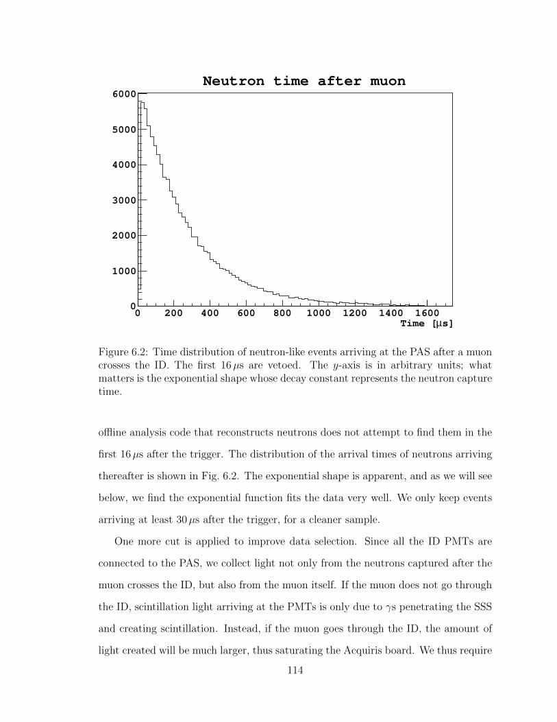
s]µTime [0 200 400 600 800 1000 1200 1400 16000

1000

2000

3000

4000

5000

6000Neutron time after muon

Figure 6.2: Time distribution of neutron-like events arriving at the PAS after a muoncrosses the ID. The first 16µs are vetoed. The y-axis is in arbitrary units; whatmatters is the exponential shape whose decay constant represents the neutron capturetime.

offline analysis code that reconstructs neutrons does not attempt to find them in the

first 16µs after the trigger. The distribution of the arrival times of neutrons arriving

thereafter is shown in Fig. 6.2. The exponential shape is apparent, and as we will see

below, we find the exponential function fits the data very well. We only keep events

arriving at least 30µs after the trigger, for a cleaner sample.

One more cut is applied to improve data selection. Since all the ID PMTs are

connected to the PAS, we collect light not only from the neutrons captured after the

muon crosses the ID, but also from the muon itself. If the muon does not go through

the ID, scintillation light arriving at the PMTs is only due to γs penetrating the SSS

and creating scintillation. Instead, if the muon goes through the ID, the amount of

light created will be much larger, thus saturating the Acquiris board. We thus require

114

that the board was saturated by the trigger, in order to ensure that we have a sample

of muons crossing the Inner Detector.

After the employment of the three cuts (neutron energy, muon through ID, ar-

rival time), we observed 70748 neutrons following 19201 neutron-producing muons. 1

Assuming the number of neutron-producing muons is subject to Poisson statistical

fluctuations [36], we have prepared a toy Monte Carlo code to calculate the statistical

uncertainties in neutron rate. The neutron multiplicity distribution for neutron-

producing muons is shown in Fig. 6.3. 2 Each Monte Carlo event picks a muon

multiplicity from a Poisson distribution centered at 19201. For each of those muons,

a neutron number is picked from the neutron distribution in Fig. 6.3. The total neu-

tron count for each muon is then used to fill a histogram. The result is shown in

Fig. 6.4. We have fitted the distribution to a Gaussian for uncertainty estimation.

The average comes out to 7.071×10−4, quite close to the actual number (70748, as

mentioned above), while the width is 1965, which we take to be our neutron uncer-

tainty.

Thus, the raw rates of neutrons and neutron-producing muons are 3

rnraw = (230.4± 6.0) d−1, (6.2)

rµraw = (61.14± 0.44) d−1,

These are known as the “raw rates” because a number of checks and corrections must

be made before a final rate can be reported.

1Throughout this Chapter, the term “muon” means “muon that produces at least one neutron”.2There is a 0.03% discrepancy between the live time reported in Sec. 6.2 and the one shown in

the y-axis of Fig. 6.3, due to a mistake in the definition of run start and end that was fixed afterthe creation of this figure, and before the evaluation of the live time in Sec. 6.2.

3For convenience, these rates already include two high-multiplicity muons that were mistakenlytagged as noise. We study those muons in Sec. 6.3.4.3.

115

Figure 6.3: Neutron multiplicity distribution in 314 d, the live time defined in Sec. 6.2.The solid line is the real distribution, which was used for the estimation of the neutronstatistical uncertainty (see text); the dashed line is re-binned so that no bin exceptthe zeroth is empty.

116

Figure 6.4: Number of neutron captures in 314.176 live days as simulated by our toyMonte Carlo.

117

6.3 Corrections

Corrections to the neutron rate will be indicated by an n superscript, while those for

muons will be indicated with a µ superscript. Some muon corrections will affect the

neutron rate, while some neutron corrections will affect the muon rate. This will be

discussed in Sec. 6.4.

6.3.1 Time-dependent DAQ efficiency

We fit the neutron capture time between 50µs and 1500µs after the muon to an

exponential, and find

τn = 261± 1µs, (6.3)

very close to previous measurements [41]. We split the DAQ time window of 30–

1590µs into three bins: 30-100µs, 100-405µs, and 405-1590µs. The probabilities

for a neutron falling in each of these time windows, based on the neutron capture

time of Eq. 6.3, are 0.236, 0.528, and 0.236, respectively. We count the number of

neutrons in each of the earliest and latest time windows. We then calculate the range

of efficiencies that can account for the discrepancies at 2σ level. Finally, we accept

the crude model of highest inefficiency at earliest times, intermediate inefficiency in

the time in between, and perfect efficiency at latest times. The resulting average

inefficiency is

ηnt−dep = 0.988± 0.006 %. (6.4)

6.3.2 Time-independent DAQ efficiency

We looked at a well-understood sample of muons from the main system, and counted

how many were also seen by the analog system. The resulting efficiency is:

ηµblind = 0.926± 0.004. (6.5)

118

The uncertainty comes from the choice of neutron cut employed in selecting the main

DAQ sample, as all selected muons are required to have produced at least one neutron.

The main source of this inefficiency has been found to be that the analog DAQ is

blind to new triggers for ∼0.16 s after every MTB trigger, hence the subscript. The

dead time induced is ∼5±1 %, which is close to the inefficiency quoted here. Further

study is required to confirm the blindness of the board, and to find the source of

the remaining inefficiency. A possible hypothesis is that excursions of the baseline

caused clusters to be missed by the online cut that threw away cluster-less events

to save disk space. Assuming, however, that most of the missed muons are due to a

dead time induced by all MTB triggers, missed muons should have the same neutron

multiplicity as found muons. This was confirmed by looking at the multiplicities in the

main DAQ, where we found no significant difference between the neutron multiplicity

distribution of matched and unmatched muons.

Neutrons following detected muons could also be missed, if the board went blind

for a few microseconds at a time. To test this, we took a very strict sample of neutrons

detected by the main system, and counted how many were seen by the analog system,

assuming matched muons. We obtained an efficiency of

ηnblind = 0.998. (6.6)

Further inefficiencies that also affect the main DAQ could be present.

119

6.3.3 DAQ time window

Using the neutron capture time, we can calculate the expected fraction of neutron

captures occurring in the DAQ time window, resulting in an efficiency of:

ηnt−window = 0.88913± 0.00032 (6.7)

ηµt−window = 0.927± 0.004

The muon efficiency was estimated based on previous work by R. Saldanha [83]: we

estimate the number of muons that produced neutrons but had none detected, based

on the probability to miss a neutron due to the finiteness of the DAQ time window,

and the distribution of neutron multiplicities per muon observed.

6.3.4 Noise cut

We employed three types of noise cut in the offline neutron reconstruction software:

the so called “ratio cut”, “variance cut” and “saturation cut” (defined below). We

found that all of them incorrectly removed some muons as well as noise events. For

all the studies described below, we looked at the noise waveforms that seemed to

contain neutrons by eye, and determined how many muon events were missed in this

way, separating them by the type of noise cut.

6.3.4.1 Ratio cut

This cut removes events when the integral of the positive part of the waveform is

more than 60% of the integral of the negative part. (most of the signal is negative, as

suggested by Fig. 6.1). We found that the muon events removed by the “ratio cut”

were removed by their very nature, indicating that the cut was poorly designed. We

studied the analog DAQ run numbers between 99230 and 99264. We calculated the

ratio of muon events labeled as noise by the ratio cut to all muon events obtained

120

during the same runs. Finally, we calculated, using the Agresti-Coull method, the

range of probabilities for this to happen assuming binomial statistical fluctuations.

We obtain a muon detection efficiency of

ηµnoise−ratio = 0.9961± 0.0016 (6.8)

This correction should also be applied to the neutron rate, assuming missed muons

have the same neutron multiplicity distribution as any other set of muons.

6.3.4.2 Variance cut

The variance cut is put in place to remove events for which the baseline oscillates

more than expected. We studied the analog DAQ run numbers between 99230 and

99264, and found that this cut removed muons only casually, when a muon event

was particularly noisy for external reasons. Because the mis-labeled muons occur

proportionally to the total number of noise triggers (as identified by these cuts), we

calculated their ratio and took it as the mean number of triggers removed by the

variance cut that are actually muons. To estimate the uncertainty in this number, we

varied this mean number and calculated the probability for observing the number of

mis-labeled muons we observed in our test sample, assuming Poisson statistics. The

resulting efficiency is

ηµnoise−variance = 0.9988+0.0007−0.0013 (6.9)

This correction should also be applied to the neutron rate, assuming missed muons

have the same neutron multiplicity distribution as any other set of muons.

121

6.3.4.3 Saturation cut

The saturation cut removed events when the waveform saturated positively without

having saturated negatively shortly before. 4 Two high-multiplicity muons were re-

moved by this cut from the entire data set considered in this analysis, for reasons

unknown at this time. By a mixture of manual counting and extrapolation using the

capture time, we found the number of neutrons following these two muons to be

Nsat cut = 1624± 26 (6.10)

The uncertainty comes from the difficulty in identifying neutrons by eye. We added

those to the raw count to obtain the rate in Eq. 6.2.

6.3.5 CNGS spills

CERN Neutrinos to Gran Sasso (CNGS) [84] can create high-energy muons, which

then can enter the detector and produce neutrons. This process can mimic a cosmo-

genic muon followed by neutron captures in the scintillator, and we must remove the

fake events. We match the analog neutron to the main DAQ using the muon time

and the neutron time after the muon. Knowing the precise timing of CNGS events

given by the beam operators, we then match the muons that are found by both the

analog and the main DAQ systems to the CNGS spills by main DAQ run and trigger

number. We assume that the fraction of all events that are CNGS spills is the same

for analog muons that are seen by the main system and for those that are not seen.

The correction is applied only for the time periods during which the CNGS beam is

4If an event saturates negatively, the board then typically turns around and saturates positivelyshortly afterward.

122

on.

ηnCNGS = 1.133± 0.003 (6.11)

ηµCNGS = 1.059+0.002−0.001

Note that these values are dependent on the live time period chosen. We could instead

remove the CNGS-tagged events from our sample, and it would be equally valid.

We need to estimate the probability for CNGS spills to be incorrectly identified,

which might incur in undetected spills, or in cosmogenic muons removed incorrectly.

The possible ways to see a CNGS spill and not properly remove it are: a CNGS spill

that was not time-labeled at the source (extremely unlikely); a CNGS spill that took

place while the main DAQ was on, but did not get recorded in the main DAQ, and did

get recorded in the analog DAQ, so we did not subtract it because the match is miss-

ing (unlikely because Borexino has extremely high efficiency for muon tagging [41]);

a CNGS spill took place while the main DAQ is off, the analog DAQ recorded it,

but the CNGS time label and the analog DAQ event are separated by more than

25 s (unlikely, because we looked at the time difference distribution between analog

and main, and between main and CNGS, and 25 s seemed like a conservative reso-

lution). The only other error that can remove a cosmogenic event mistaking it for

a CNGS spill is if a cosmogenic muon event took place near a CNGS spill, and the

analog event was incorrectly matched to a main event that was correlated with a

CNGS spill. The effect of this error can be estimated as follows: the mean number

of neutron-producing muons in 25 s is 0.02 (see Eq. 6.15); we have ∼1500 CNGS

spills; 5 therefore, the total number of times this could have happened is ∼30, which

would not modify the efficiency due to CNGS spills significantly. Furthermore, both

over-counting and under-counting could take place due to mistakes in the match-

5Since the acquisition window is ∼1.6 ms (Sec. 6.3.1), a removal of ∼1500 muons corresponds toa negligible time adjustment of ∼2 s (see Eq. 6.1)

123

ing algorithm between main and analog DAQs, but we have already evaluated the

matching efficiency elsewhere.

6.3.6 Volume

The volume of the Borexino inner vessel (IV) changed considerably during the DAQ

time period, due to buoyancy force and the inner vessel leak [33]. Values oscillated

in the range given by V = 310 ± 5 m3, which after scaling for the density of the

scintillator [33] gives a mass range of

m = 273± 4 t. (6.12)

The nominal Borexino mass is 278 t [54]. If we quote our rate in (d×278 t), the

effective volume efficiency is

ηµ,nvol = 0.98± 0.02 (6.13)

6.3.7 Energy cut

The energy cut was placed at 1.3 MeV because it had been the choice of previous

preliminary studies [85]. However, it is likely that some neutrons that deposited less

energy were missed by this cut. We have employed a MC simulation of neutron cap-

tures uniformly distributed throughout the Stainless Steel Sphere (SSS) of Borexino.

The γs produced by the neutron captures are then emitted in random directions. The

simulation returns the amount of energy deposited in the inner vessel by the capture

γs. No electronics effects are simulated, as the analog DAQ electronics have not been

implemented in the simulation package g4bx (see Chapter 3), which we used for this

study. We count the total number of events that deposit more than 1.3 MeV inside

the IV and divide by the total number of events produced inside the IV, resulting in

124

an efficiency of

ηE cut = 0.982+0.009−0.010 (6.14)

The systematic uncertainty, due to electronics effects, is estimated by looking at the

charge distribution as measured by the analog DAQ of the events that just barely

pass the energy cut as defined by pulse height. The additional uncertainty, coming

from the error in the simulation, is negligible.

6.3.8 High-energy depositions

We investigated the possibility that high-energy clusters are not due to neutron cap-

tures on hydrogen. There is a number of events (1.0%) with energies larger than

3.2 MeV, well beyond the tail of the 2.2 MeV γ peak. These events have previously

been studied in [85], where they concluded that ∼60% were caused by neutron cap-

tures on carbon, while the remaining 40% were caused by pile-up of captures on H.

Given that we want to give our final neutron rate for captures on hydrogen only, the

inclusion of this tail results in an over-efficiency, corresponding to 20% of the counts

in the high-energy region (the other two 40%’s cancel each other). The correction is

therefore on the order of a fifth of 1%, which is negligible.

6.4 Results and conclusions

We apply all the corrections and uncertainties listed in Sec. 6.3, and summarized in

Tab. 6.1. Neutron corrections affect muon rates indirectly, since a missed neutron can

result in a missed muon. We have neglected this second-order correction except in

the case of the DAQ time window correction. Muon corrections affect neutron rates

in a more straightforward way: assuming the neutron multiplicity distribution is the

same for all muon samples, then the inefficiency in muon detection can be directly

125

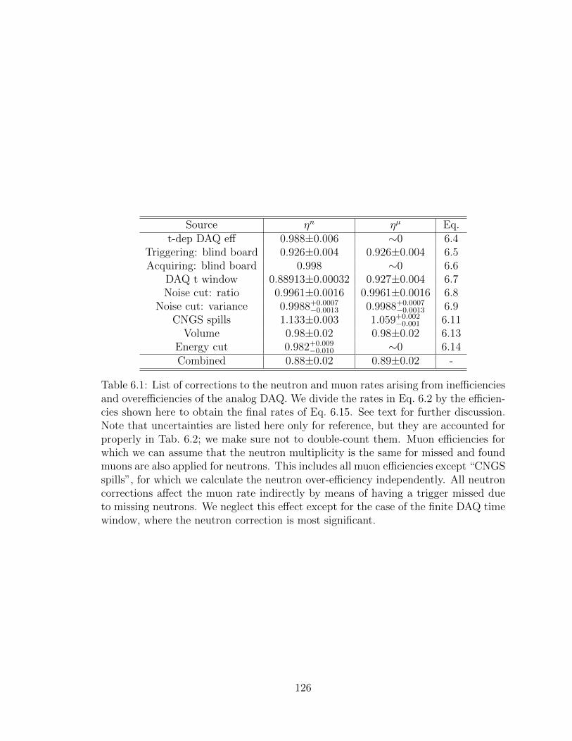
Source ηn ηµ Eq.t-dep DAQ eff 0.988±0.006 ∼0 6.4

Triggering: blind board 0.926±0.004 0.926±0.004 6.5Acquiring: blind board 0.998 ∼0 6.6

DAQ t window 0.88913±0.00032 0.927±0.004 6.7Noise cut: ratio 0.9961±0.0016 0.9961±0.0016 6.8

Noise cut: variance 0.9988+0.0007−0.0013 0.9988+0.0007

−0.0013 6.9CNGS spills 1.133±0.003 1.059+0.002

−0.001 6.11Volume 0.98±0.02 0.98±0.02 6.13

Energy cut 0.982+0.009−0.010 ∼0 6.14

Combined 0.88±0.02 0.89±0.02 -

Table 6.1: List of corrections to the neutron and muon rates arising from inefficienciesand overefficiencies of the analog DAQ. We divide the rates in Eq. 6.2 by the efficien-cies shown here to obtain the final rates of Eq. 6.15. See text for further discussion.Note that uncertainties are listed here only for reference, but they are accounted forproperly in Tab. 6.2; we make sure not to double-count them. Muon efficiencies forwhich we can assume that the neutron multiplicity is the same for missed and foundmuons are also applied for neutrons. This includes all muon efficiencies except “CNGSspills”, for which we calculate the neutron over-efficiency independently. All neutroncorrections affect the muon rate indirectly by means of having a trigger missed dueto missing neutrons. We neglect this effect except for the case of the finite DAQ timewindow, where the neutron correction is most significant.

126

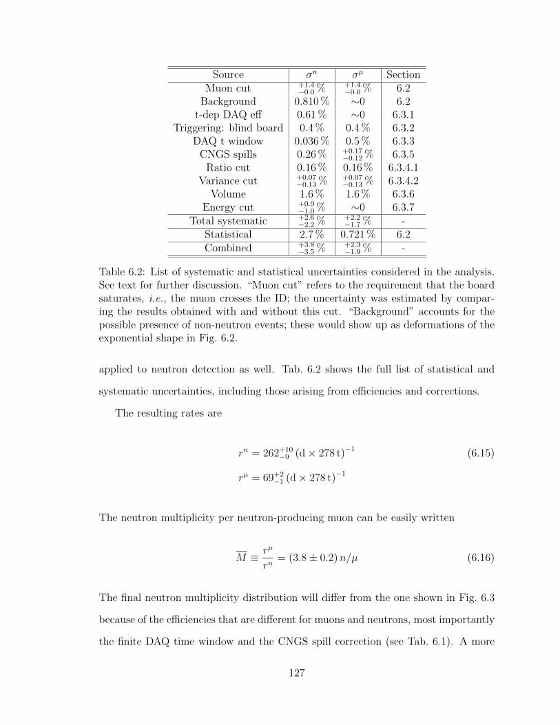
Source σn σµ SectionMuon cut +1.4

−0.0 % +1.4−0.0 % 6.2

Background 0.810 % ∼0 6.2t-dep DAQ eff 0.61 % ∼0 6.3.1

Triggering: blind board 0.4 % 0.4 % 6.3.2DAQ t window 0.036 % 0.5 % 6.3.3

CNGS spills 0.26 % +0.17−0.12 % 6.3.5

Ratio cut 0.16 % 0.16 % 6.3.4.1Variance cut +0.07

−0.13 % +0.07−0.13 % 6.3.4.2

Volume 1.6 % 1.6 % 6.3.6Energy cut +0.9

−1.0 % ∼0 6.3.7Total systematic +2.6

−2.2 % +2.2−1.7 % -

Statistical 2.7 % 0.721 % 6.2Combined +3.8

−3.5 % +2.3−1.9 % -

Table 6.2: List of systematic and statistical uncertainties considered in the analysis.See text for further discussion. “Muon cut” refers to the requirement that the boardsaturates, i.e., the muon crosses the ID; the uncertainty was estimated by compar-ing the results obtained with and without this cut. “Background” accounts for thepossible presence of non-neutron events; these would show up as deformations of theexponential shape in Fig. 6.2.

applied to neutron detection as well. Tab. 6.2 shows the full list of statistical and

systematic uncertainties, including those arising from efficiencies and corrections.

The resulting rates are

rn = 262+10−9 (d× 278 t)−1 (6.15)

rµ = 69+2−1 (d× 278 t)−1

The neutron multiplicity per neutron-producing muon can be easily written

M ≡ rµ

rn= (3.8± 0.2)n/µ (6.16)

The final neutron multiplicity distribution will differ from the one shown in Fig. 6.3

because of the efficiencies that are different for muons and neutrons, most importantly

the finite DAQ time window and the CNGS spill correction (see Tab. 6.1). A more

127

complete study of the neutron multiplicity distribution, including comparisons to

Monte Carlo simulations, can be found in [44].

We are also interested in the number of neutrons per unit muon track length, or

neutron yield, given by:

Yn =rn

ρ× (4/3)R× φµ × A, (6.17)

where ρ is the density of the scintillator, and R is the radius of the volume of neutron

detection. Such volume is obtained from simulation, as the point where the neutron

detection efficiency becomes 0.5, and is equal to 4.19 m. The actual value of the radius

during the time period used for this analysis is 4.20±0.02 m (Sec. 6.3.6), consistent

with the value found by the simulation. φµ is the muon flux as measured by Borexino

((3.41±0.01)·10−4/m2/s) [44], and A is the largest cross-sectional area of the detection

sphere. Since we are only sensitive to muons crossing the IV, A will be given by the

radius R. Using the density of 0.88 g/cm3 [83], we obtain:

Yn = (3.19± 0.08 (stat)+0.09−0.08 (syst)± 0.01 (flux))× 10−4 n/(µ · g/cm2)

All results are consistent with those found by the main Borexino DAQ [44]. These

results were used to tune the Monte Carlo simulation packages Geant4 and Fluka,

which are extensively used for direct dark matter detection experiment design. They

have also been useful to demonstrate the feasibility of second-generation dark matter

detectors at Gran Sasso depths [86].

128

Appendix A

Glossary

In this chapter, we define some important acronyms and terms used throughout thethesis.

• BTB: Borexino Trigger Board. See Sec. 2.3.

• CTF: Counting Test Facility. See Sec. 2.1.

• DAQ: Data Acquisition. The process of registering and storing data in Borexino.

• Dark Rate: rate of PMT hits coming from unidentified random sources, i.e.,Dark Noise.

• DN: Dark Noise. The signals registered by a PMT in Borexino that are not dueto physics events in the detector.

• Echidna: The Borexino low-to-high level reconstruction code. See Sec. 2.3.

• ID: Inner Detector. See Sec. 2.

• IDF: Inner Detector Flag. See Sec. 2.3.

• FV: Fiducial Volume. The virtual volume inside which we accept scintillationevents as candidate neutrino interactions. See Sec. 2.2.

• M4: Mach4.

• Mach4: An alternative to Echidna. See Sec. 2.3. The term is also used inter-changeably for MOE.

• MC: Monte Carlo, a class of computational methods commonly used for physicsevent simulation. Also used as a synonym for “simulation” or “simulated”. SeeChapter 3.

129

• MCR: Muon Cluster Flag. See Sec. 2.3.

• MOE: Mach4 Over Echidna. See Sec. 2.3.

• Monte Carlo: see MC.

• MTB: Muon Trigger Board. See Sec. 2.3.

• MTF: Muon Trigger Flag. See [41].

• OD: Outer Detector. See Sec. 2.

• PAS: Princeton Analog System. See Sec. 2.3.1 and Chapter 6.

• Phototube: PMT.

• PMT: Photomultiplier Tube. A device that detects photons through the pho-toelectric effect [87].

• simulator: a program that generates the analytical shapes of the species in-cluded in the fit. See Sec. 2.8.

• spectral-fitter: a program that performs a spectral fit of the data usingbackground and signal components input by the user. See Sec. 2.8.

• WIMP: Weakly Interacting Massive Particle. See Chapter 6.

• WT: Water Tank. See Chapter 2

130

Bibliography

[1] Laurie M. Brown. The idea of the neutrino. Physics Today, 31:23, 1978.

[2] C. L. Cowan, F. Reines, F. B. Harrison, H. W. Kruse, and A. D. McGuire.Detection of the free neutrino: a confirmation. Science, 124(3212):103–104, 1956,http://www.sciencemag.org/content/124/3212/103.full.pdf.

[3] P. A. R. Ade et al. Planck 2013 results. XVI. Cosmological parameters. submittedto Astronomy & Astrophysics, March 2013, arXiv:1303.5076.

[4] David Griffiths. Introduction to Elementary Particles. Wiley-VCH, 2 edition,2008.

[5] James W. Cronin and Margaret Stautberg Greenwood. Cp symmetry violation.Physics Today, 35:38, 1982.

[6] K. Nakamura and S.T. Petcov. Neutrino mass, mixing, and oscillations. Technicalreport, Particle Data Group, 2012.

[7] S. Sambursky. The Physical World of Greeks. Collier Books, 1962.

[8] Hermann Hunger and David Pingree. Astral Sciences in Mesopotamia. Brill,1999.

[9] H. A. Bethe. Energy production in stars. Phys. Rev., 55:434–456, March 1939.

[10] John N. Bahcall. Neutrino Astrophysics. Cambridge University Press, 1989.

[11] Donald D. Clayton. Principles of Stellar Evolution and Nucleosynthesis. Chicago,1983.

[12] John N. Bahcall. Solar neutrino viewgraphs, 2005. http://www.sns.ias.edu/

~jnb/SNviewgraphs/snviewgraphs.html.

[13] G. Bellini et al. First evidence of pep solar neutrinos by direct detection inBorexino. Phys.Rev.Lett., 108:051302, 2012, arXiv:1110.3230.

[14] G. Bellini et al. Precision Measurement of the 7Be Solar Neutrino InteractionRate in Borexino. Phys.Rev.Lett., 107:141302, September 2011, arXiv:1104.

1816.

131

[15] G. Bellini et al. Measurement of the solar 8B neutrino rate with a liquid scintil-lator target and 3 MeV energy threshold in the Borexino detector. Phys. Rev.D, 82:033006, August 2010.

[16] F.L. Villante, A. Ianni, F. Lombardi, G. Pagliaroli, and F. Vissani. A steptoward CNO solar neutrino detection in liquid scintillators. Physics Letters B,701(3):336 – 341, 2011.

[17] Aldo M. Serenelli, W. C. Haxton, and Carlos Pena-Garay. Solar Models withAccretion. I. Application to the Solar Abundance Problem. The AstrophysicalJournal, 743(1):24, 2011.

[18] John N. Bahcall, Marc Kamionkowski, and Alberto Sirlin. Solar neutrinos: Ra-diative corrections in neutrino-electron scattering experiments. Phys. Rev. D,51:6146–6158, June 1995.

[19] Michael E. Peskin and Daniel V. Schroeder. An Introduction to Quantum FieldTheory. Westview Press, 1995.

[20] Ch. Kraus, B. Bornschein, L. Bornschein, J. Bonn, B. Flatt, A. Kovalik, B. Os-trick, E.W. Otten, J.P. Schall, Th. Thummler, and Ch. Weinheimer. Final resultsfrom phase II of the Mainz neutrino mass searchin tritium β decay. The EuropeanPhysical Journal C - Particles and Fields, 40(4):447–468, 2005.

[21] Raymond Davis, Don S. Harmer, and Kenneth C. Hoffman. Search for neutrinosfrom the sun. Phys.Rev.Lett., 20:1205–1209, May 1968.

[22] S.P. Mikheyev and A.Yu. Smirnov. Resonant amplification of oscillations inmatter and solar-neutrino spectroscopy. Il Nuovo Cimento C, 9(1):17–26, 1986.

[23] Q. R. Ahmad et al. Measurement of the Rate of νe + d → p + p + e− Inter-actions Produced by 8B Solar Neutrinos at the Sudbury Neutrino Observatory.Phys.Rev.Lett., 87:071301, July 2001.

[24] Y. Fukuda et al. Evidence for oscillation of atmospheric neutrinos.Phys.Rev.Lett., 81:1562–1567, August 1998.

[25] S. Eidelman et al. Review of particle physics. Physics Letters B, 592(14):1 – 5,2004.

[26] A. Aguilar et al. Evidence for neutrino oscillations from the observation of νeappearance in a νµ beam. Phys. Rev. D, 64:112007, November 2001.

[27] A. A. Aguilar-Arevalo et al. Event Excess in the MiniBooNE Search for νµ → νeOscillations. Phys.Rev.Lett., 105:181801, October 2010.

[28] C. Zhang, X. Qian, and P. Vogel. Reactor antineutrino anomaly with known θ13.Phys. Rev. D, 87:073018, April 2013.

132

[29] Joachim Kopp, Pedro A.N. Machado, Michele Maltoni, and Thomas Schwetz.Sterile neutrino oscillations: the global picture. Journal of High Energy Physics,2013(5):1–52, 2013.

[30] G. Bellini et al. SOX: Short distance neutrino Oscillations with BoreXino. Jour-nal of High Energy Physics, 2013(8):1–14, 2013, arXiv:1304.7721.

[31] G. Alimonti et al. The Borexino detector at the Laboratori Nazionali delGran Sasso. Nuclear Instruments and Methods in Physics Research Section A,600(3):568 – 593, 2009.

[32] Michael Leung. The Borexino Solar Neutrino Experiment: Scintillator Purifica-tion and Surface Contamination. PhD thesis, Princeton University, 2006.

[33] Richard Saldanha. Precision measurement of the 7Be solar neutrino interactionrate in Borexino. PhD thesis, Princeton University, 2011.

[34] Glenn F. Knoll. Radiation Detection and Measurement. John Wiley & Sons,Inc., 1999.

[35] A. Grau Malonda and A. Grau Carles. The ionization quench factor in liquid-scintillation counting standardizations. Applied Radiation and Isotopes, 51:183–188, 1999.

[36] G. Bellini. Final results of Borexino Phase-I on low energy solar neutrino spec-troscopy. accepted for publication in Phys. Rev. D, 2013, arXiv:1308.0443.

[37] Jose M. Los Arcos and Felix Ortiz. kB: a code to determine the ionizationquenching function Q(E) as a function of the kB parameter. Computer PhysicsCommunications, 103(1):83 – 94, 1997.

[38] C. Arpesella et al. Measurements of extremely low radioactivity levels inBOREXINO. Astroparticle Physics, 18(1):1 – 25, 2002.

[39] G. Bellini. The Borexino experiment and the results of the Counting Test Facility.Nuclear Physics B (Proc. Suppl.), 48:363–369, 1996.

[40] G. Alimonti et al. Light propagation in a large volume liquid scintillator. NuclearInstruments and Methods in Physics Research Section A, 440(2):360 – 371, 2000.

[41] G. Bellini et al. Muon and cosmogenic neutron detection in Borexino. Journalof Instrumentation, 6(05):P05005, 2011.

[42] Davide D’Angelo. Towards the detection of low energy solar neutrinos inBOREXino: data readout, data reconstruction and background identification.PhD thesis, Technische Universitat Munchen, 2006.

[43] F. Gatti, V. Lagomarsino, P. Musico, M. Pallavicini, A. Razeto, G. Testera,and S. Vitale. The Borexino read out electronics and trigger system. NuclearInstruments and Methods in Physics Research Section A, 461:474–477, 2001.

133

[44] G. Bellini et al. Cosmogenic Backgrounds in Borexino at 3800 m water-equivalentdepth. JCAP, 08:049, 2013, arXiv:1304.7381.

[45] Alex Wright, Pablo Mosteiro, Ben Loer, and Frank Calaprice. A highly efficientneutron veto for dark matter experiments. Nuclear Instruments and Methods inPhysics Research Section A, 644(1):18 – 26, 2011.

[46] A. Empl and R. Jasim and E. Hungerford and P. Mosteiro. Study of CosmogenicNeutron Backgrounds at LNGS. arXiv:1210.2708, 2012.

[47] G. Bohm and G. Zech. Statistics of weighted Poisson events and its applications.Nuclear Instruments and Methods in Physics Research Section A, 748:1–6, June2014, arXiv:1309.1287.

[48] Oleg Yu. Smirnov. Testing the scintillation line shape. Borexino internal note,http://borex.lngs.infn.it/papers/public.shtml, December 2013.

[49] O. Yu. Smirnov. An approximation of the ideal scintillation detector line shapewith a generalized gamma distribution. Nuclear Instruments and Methods inPhysics Research Section A, 595(2):410 – 418, 2008.

[50] M.J. Berger, J.S. Coursey, M.A. Zucker, and J. Chang. Stopping-power andrange tables for electrons, protons, and helium ions. Online NISTIR 4999, NIST,Physical Measurement Laboratory, 2005. http://physics.nist.gov/Star.

[51] Packard Instrument Company. The effect of quench on quantitating alpha ra-dionuclides by liquid scintillation counting. http://www.perkinelmer.com/

CMSResources/Images/44-73008APP_ABAQuenchQuantAlphaRadionucl.pdf.

[52] C. Galbiati and K. McCarty. Time and space reconstruction in optical, non-imaging, scintillator-based particle detectors. Nuclear Instruments and Methodsin Physics Research Section A, 568(2):700 – 709, 2006.

[53] G. Alimonti et al. Ultra-low background measurements in a large volume under-ground detector. Astroparticle Physics, 8(3):141 – 157, 1998.

[54] H. Back et al. Borexino calibrations: hardware, methods, and results. Journalof Instrumentation, 7, 2012, arXiv:1207.4816.

[55] John N. Bahcall. Software and data for solar neutrino research. Technical report,Institute for Advanced Study, 2005. http://www.sns.ias.edu/~jnb/SNdata/

sndata.html Accessed on 2013-09-29.

[56] P.C. de Holanda, Wei Liao, and A.Yu. Smirnov. Toward precision measurementsin solar neutrinos. Nuclear Physics B, 702(307–332), 2004.

[57] L.P. Ekstrom and R.B. Firestone. WWW Table of Radioactive Isotopes.Database version 2/28/99, LBNL Isotopes Project - LUNDS Universitet, 1999.http://ie.lbl.gov/toi/.

134

[58] V.V.Kuzminov and N.Ja.Osetrova. Precise Measurement of 14C Beta Spectrumby Using a Wall-less Proportional Counter. Physics of Atomic Nuclei, 63(7),2000.

[59] Masato Morita. Beta decay and muon capture. W.A. Benjamin, Inc., Reading,Massachusetts 01867, U.S.A., 1973.

[60] J.L.Mortara, I.Ahmad, S.J.Freedman, B.K.Fujikaw, and J.P.Greene. Test of theconserved vector current hypothesis in the β-decay of 14C. ANL report.

[61] F. E. Wietfeldt et al. Further studies on the evidence for a 17-kev neutrino in a14doped [sic] germanium detector. Phys. Rev. C, 52:1028–1040, August 1995.

[62] European Nuclear Society. Decay chains, natural. Technical report, EuropeanNuclear Society, 2014. http://www.euronuclear.org/info/encyclopedia/d/decaybasinnatural.htm.

[63] Richard B. Firestone. The Berkeley Laboratory Isotopes Project. LBNL, 2008.

[64] O. Smirnov. Update of the 7be analysis. Borexino Internal Memo, 2008.

[65] G. Keefer and A. Piepke. Beta spectra for 39ar, 85kr, and 210bi. http://bama.

ua.edu/~andreas/ps_files/beta.pdf, May 2004.

[66] A. Grau Carles and K. Kossert. New advances in the determination of the 87rbshape factor function. Nuclear Physics A, 767:248–258, 2006.

[67] Mark Winter. Abundance in earth’s crust: periodicity. Technical report, TheUniversity of Sheffield, 2012. http://www.webelements.com/periodicity/

abundance_crust/ Accessed on 2014-03-06.

[68] S. Agostinelli et al. Geant4A simulation toolkit. Nuclear Instruments and Meth-ods in Physics Research Section A, 506(3):250 – 303, 2003.

[69] G. Bellini et al. First direct observation of the neutrinos from primary proton-proton fusion in the sun. submitted to Nature, 2014.

[70] G. Bellini et al. Absence of a day-night asymmetry in the 7Be solar neutrino ratein Borexino. Physics Letters B, 2011.

[71] Keith Otis. Direct measurement of the pp solar neutrino interaction rate inBorexino. PhD thesis, University of Massachusetts Amherst, 2014.

[72] Lorenzo Moneta, Fred James, Matthias Winkler, and Andras Zsenei. Minuit,2008. http://lcgapp.cern.ch/project/cls/work-packages/mathlibs/minuit/.

[73] H. Daniel. Das β-spektrum des RaE. Nuclear Physics, 31(0):293 – 307, 1962.

[74] D. Flothmann, W. Wiesner, R. Lohken, and H. Rebel. β-Spektroskopie mitHalbleiterdetektoren beim Zerfall von 32P, 49Sc, 204Tl und 210Bi. Z. Physik,225:164–194, 1969.

135

[75] J. N. Bahcall, P. I. Krastev, and A. Yu. Smirnov. Where do we stand with solarneutrino oscillations? Phys. Rev. D, 58(096016), 1998.

[76] J.N. Bahcall, P.I. Krastev, and A.Yu. Smirnov. Is Large Mixing Angle MSWthe Solution of the Solar Neutrino Problems? Phys. Rev. D, 60:093001, October1999.

[77] G. L. Fogli, E. Lisi, A. Marrone, D. Montanino, A. Palazzo, and A. M. Rotunno.Global analysis of neutrino masses, mixings, and phases: Entering the era ofleptonic CP violation searches. Phys. Rev. D, 86:013012, July 2012, arXiv:

1205.5254.

[78] Aldo Ianni, Livia Ludhova, and Alessandra Carlotta Re. pp-ν: theoretical ex-pectations and experimental values for solar flux, survival probability, and inter-action rate. Borexino internal note, April 2014.

[79] George A. Cowan and Wick C. Haxton. Solar variability: Glacial epochs, andsolar neutrinos. Los Alamos Science, Summer 1982.

[80] G. Bellini et al. Cosmic-muon flux and annual modulation in Borexino at 3800 mwater-equivalent depth. JCAP, 1205:015, 2012, arXiv:1202.6403.

[81] Rene Brun and Fons Rademakers. ROOT - An Object Oriented Data AnalysisFramework. In Proceedings AIHENP’96 Workshop, Lausanne, Sep. 1996, volume389, pages 81–86, 1997.

[82] Daniela Pantosti. The L’Aquila seismic sequence - April 2009. Istituto Nazionaledi Geofisica e Vulcanologia, August 2009. http://www.webcitation.org/

5jc8Veudk.

[83] Richard N. Saldanha. Reduction of 11C background in Borexino. Pre-ThesisProject, January 2009.

[84] CERN. CNGS Project. Technical report, CERN, 2012. http://proj-cngs.

web.cern.ch/proj-cngs/.

[85] Alvaro E. Chavarrıa. Neutron detection in Borexino. Experimental Project,November 2008.

[86] D. Bauer et al. WIMP Dark Matter Direct Detection. arXiv:1310.8327, October2013.

[87] Editorial Committee. Photomultiplier tubes: Basics and applications. TechnicalReport 3a, Hamamatsu Photonics K.K., 2007.

136