pramod k. singh and abhishek nair - irma | home · 2013-09-02 · pramod k. singh and abhishek nair...

Working Paper 248

CLIMATE CHANGE VULNERABILITY

ASSESSMENT FOR SUSTAINABLE

LIVELIHOODS USING FUZZY COGNITIVE

MAPPING APPROACH

Pramod K. Singh and Abhishek Nair

The purpose of the Working Paper Series (WPS) is to provide an

opportunity to IRMA faculty, visiting fellows, and students to sound out

their ideas and research work before publication and to get feedback

and comments from their peer group. Therefore, a working paper is to

be considered as a pre-publication document of the Institute.

Institute of Rural Management Anand

Post Box No. 60, Anand, Gujarat (India)

Phones: (02692) 263260, 260246, 260391, 261502

Fax: 02692-260188 Email: [email protected]

Website: www.irma.ac.in

June 2013

http://www.irma.ac.in/

1

Climate Change Vulnerability Assessment for Sustainable Livelihoods using

Fuzzy Cognitive Mapping Approach

Pramod K. Singh1 and Abhishek Nair

2

Abstract

In order to move towards climate resilient pathways local vulnerability assessments based

on peoples’ perception are required where there are large data constraints. In this paper

we have developed a new climate change vulnerability index for sustainable livelihoods to

estimate the vulnerability of poor agro-pastoralists in the Bhilwara and Tonk districts of

Rajasthan, India. The existing studies of livelihood vulnerability assessments often do not

capture the dynamics and functioning of interconnected systems. We used a semi-

quantitative fuzzy cognitive mapping approach to understand interconnected interactions

occurring in the climate-human-environment interaction space. This approach enables the

quantification of peoples’ perceptions of perturbations to a given climate exposure and

their adaptation mechanisms in relative terms. This was combined with a sustainable

livelihood approach for an improved understanding of asset classes sensitive to climate

change and assets serving as adaptive capacities. Data collection involved group

discussions during which 35–38 groups drew cognitive maps in each district on climate-

related perturbations and adaptation mechanisms. Data from cognitive maps were

aggregated using a composite index and differential vulnerabilities were compared.

Results indicate that Tonk may be more vulnerable to climate change due to lower

adaptive capacity than Bhilwara over all three seasons. Asset classes most susceptible to

harm are natural assets while physical assets serve as a strong adaptive mechanism

against climate change in both the districts.

Keywords: Vulnerability, adaptation, fuzzy cognitive mapping, livelihoods

1 Associate Professor, Institute of Rural Management, Anand-388001, Gujarat, India

E-mail : [email protected] 2 Research Associate, Institute of Rural Management, Anand-388001, Gujarat, India

E-mail: [email protected]

mailto:[email protected]

mailto:[email protected]

2

1. INTRODUCTION

The climate-change issue is global and long-term, involving complex interactions between

climatic, socio-economic, environmental, technological, institutional, and political

processes. With livelihoods being increasingly affected by climate change; Cruz et al.

(2007) and Stern (2007) have stated that it adversely impacts people’s health, safety, and

livelihoods with the poor people in poor countries expected to suffer first and foremost.

Agriculture-based livelihoods are among the sectors most impacted by climate change.

Rural people in the Asia-Pacific region face serious loss of high-value agricultural lands,

significant land degradation, and reduced crop yields owed to increasing temperatures

and varying precipitation patterns (IFAD and The Global Mechanism 2009).

Climate change is already threatening agriculture-based livelihoods in Rajasthan along

with escalating competition for resources including water, land and energy from non-

agricultural sectors concomitant with a rising food demand (Government of Rajasthan

2011). Climate change projections for Rajasthan under the A1B SRES scenario for the

near-term of 2021–2050 project temperature increases by around 2–2.5ºC

(Gopalakrishnan et al. 2011) and overall rainfall reduction could lead to water shortages

(Singh et al., 2010). Several studies have explicated the seriousness of recurring droughts

in the region with far-reaching and deep impact on local livelihoods. (Sivakumar and

Kerbart 2004; Government of Rajasthan 2011). In order to increase the resilience of

livelihoods based on agriculture there is a need to understand local vulnerability of the

poor for improved adaptability to climate change.

Today, climate change vulnerability analysis incorporates several aspects of livelihood

frameworks (Schroter et al. 2005; Eakin and Bojorquez-Tapia 2008; Park et al. 2009;

Orencio and Fujii 2013; Li, Y et al., 2013). Studies are increasingly documenting the local

knowledge vis-à-vis climate change and climate variability, its impacts, and locally

developed knowledge and practices of resource use (Hennessey et al. 2007; Green et al.

2010; Leonard et al. 2013). Throughout the world, peoples’ perceptions concerning

impacts of climate change and adaptation strategies are under discussion with

governments and intergovernmental and non-governmental organisations (Hunter and

Leonard, 2010; Petheram et al. 2010; Leonard et al. 2013). Most vulnerability assessment

studies have been conducted on a macro scale in India (Obrien et al. 2004, ISNC 2008;

INCAA 2011). Local vulnerability assessments capable of capturing the dynamics of an

interconnected interacting system need to be identified against a set of indicators that

gauge vulnerability as an outcome of various factors. Since there is a lack of data and

scientific knowledge of vulnerability on a local scale, we proposed presenting the

vulnerability of two districts (Bhilwara and Tonk) in Rajasthan based on peoples’

perceptions through a multi-step fuzzy cognitive mapping (FCM) approach. This

vulnerability assessment yields relative values. FCM approach is a semi-quantitative tool

(Kosko 1986; Ozesmi and Ozesmi 2004; Vliet et al. 2009; Reckien et al. 2010) that

enables capturing the interconnected interactions in a climate-human-environment system

to depict vulnerability.

3

It is important to understand communities and their forms of adaptation, as each

adaptation option and decisions about governance and institutional arrangements are

underpinned by a set of values associated to certain worldviews that shape what is

considered to be worthwhile adaptation action and what is not (Spence et al. 2011; Wolf

and Moser 2011; Jacob et al. 2010; Leonard et al. 2013). In this study the FCM approach

has been used for the documentation of peoples’ understanding of perturbations due to

climate change and adaptation mechanisms. The remainder of the paper provides a brief

overview of the evolution of vulnerability analysis in the context of climate change.

Proceeding on to discuss the FCM approach and building the climate change vulnerability

index for sustainable livelihoods we have outlined our research findings structured into

analysis of the cognitive maps, tacit knowledge of climate related perturbations and

adaptation mechanisms, and the vulnerability of the region.

1.1. VULNERABILITY ANALYSIS: EVOLUTION AND PRACTICE

Climate change brandishes interactions between the environment and humans rendering

it a complex socio-ecological system. Vulnerability arising from climate change is often in

a continuous state of flux; both the biophysical and social processes that shape local

conditions and the ability to cope are themselves dynamic (O’Brien et al. 2005).

Vulnerability includes exposure, sensitivity to perturbations, and the capacity to adapt

(Adger 2006). Vulnerability assessments have evolved through time; the risk hazard (RH)

model of vulnerability assessment is well-represented in the work of the Intergovernmental

Panel on Climate Change. These approaches tend to consider negative outcomes as

functions of both biophysical risk factors and the 'potential for loss' of a specific exposed

population (Eakin and Luers 2006). Further investigation into the RH models reveals the

inadequacy of capturing the dynamics of a system functioning. Vulnerability in RH models

has been discussed as a linear process and as an outcome of factors that begins with

exposure and determines sensitivity or potential impacts (Burton et al. 1978; Cutter 1996;

Mustafa 1998; Brooks et al. 2005).

Vulnerability assessments that subsequently evolved into the 'Pressure and Release'

(PAR) models as defined by Blaike et al. (1994), is a function of the perturbation, stressor,

or stress, and the vulnerability of the exposed unit. This model emphasises the underlying

causes of disaster and the social production of risk (Blaike et al. 1994; Turner et al. 2003a;

Eakin and Luers 2006). Besides the dimensions of RH models, the PAR model

incorporates facets of political economy and political ecology. These perspectives focus on

the political dimensions of vulnerability while highlighting social inequities and points of

conflict within societies (Eakin and Luers 2006). The PAR model does not address issues

pertaining to resilience and the system’s ability to bounce back from perturbation in a

coupled human-biophysical system. Vulnerability assessments need to be comprehensive;

the PAR model does not encompass interactions between human-ecological systems.

According to Turner et al. (2003a) the PAR model seems insufficient for the broader

concerns of sustainability science. Ecological resilience enters vulnerability analysis and

4

views it as a coupled human-biophysical system in which both systems interact and are

interconnected with one another. Eakin and Luers (2006) claim that vulnerability is seen as

the dynamic property of a system in which humans are constantly interacting with the

biophysical environment. Ecological resilience is used to characterise a system’s ability to

rebound, absorb change and disturbance, and yet maintain a reference state after

disturbance (Hollings 1996; Turner et al. 2003a). Incorporating ecological resilience is

critical to vulnerability analysis since it tries to capture 'real vulnerability'.

The amalgam of ecological resilience and political economy with hazards has thus

addressed the concerns of vulnerability. Previous studies have confirmed that assessing

vulnerability in a system is often difficult and intricate (Cutter et al. 2003; Eakin and Luers

2006) with no single approach established yet (UNEP 2002; Orencio and Fujii 2013). A

diverse set of approaches, methods, and tools allow for a systematic integration and

investigation of interactions between humans and their social and biophysical environment

in the light of exposure, sensitivity, and adaptive capacity (Turner et al. 2003a; Turner et

al. 2003; O’Brien et al., 2004; Vincent, 2004; Brooks et al. 2005; Polsky et al. 2007; Eakin

and Bojorquez-Tapia 2008; Hahn et al. 2009). The key differences between studies

include scale, selection methods, group and aggregate indicators, and methods for

displaying results (Hahn et al. 2009). In recent years, an indicator and metrics based

analysis has been linking system dynamics quantitatively. For example, Luers et al.

(2003b) tried to link biophysical and economic attributes to vulnerability outcomes. Global

environmental change demands research indicator based analysis in policy circles for

identifying, ranking, or distinguishing between units of analysis for informing resource

allocation or targeting support programmes or other inter entions ( akin and Bo o r ue -

Tapia 2008). Vulnerability assessments, which use indicators, have been conducted at

national (Cutter et al. 2000; Moss et al. 2001; O’ Brien et al. 2004; Brooks et al. 2005) and

household levels (Alwang et al. 2001; Vincent 2007; Eakin and Bojorquez-Tapia 2008;

Hahn et al. 2009). These vulnerability assessments link attributes to outcomes without

capturing the true essence of an interacting system. The main problem with these

vulnerability assessments is the lack of interconnectedness between attributes.

1.2. Livelihood Vulnerability Analysis in the Climate Context

Political ecology, ecological resilience, and sustainable livelihood approaches have all

proved effective in identifying vulnerable systems. The sustainable livelihood approach

allows identifying the sensitivity of assets and entitlements and critical assets for coping

with and adapting to risks, and the linking of livelihood strategies to opportunities and

constraints of the broader institutional and biophysical environment (Kelly and Adger 2000;

Eakin and Luers 2006). Several studies have incorporated or combined the sustainable

livelihood approach in vulnerability analysis, which provides general lessons concerning

the varying implications of socioeconomic and environmental shocks. Besides, it is useful

for understanding the advantages of certain strategies and combinations of assets for

addressing risks (Vasquez-Leon et al. 2003; Eakin 2005; Eakin and Bojorquez-Tapia

2008; Li et al. 2013; Gautham et al. 2013; Orencio and Fujii 2013).

5

Hahn et al. (2009) developed a climate change vulnerability index based on a set of

indicators and collected data using structured questionnaires to understand vulnerability of

livelihoods to climate change. The indicators portraying vulnerability are rigid and do not

clearly showcase interactions in the system. The indicators have been aggregated and the

IPCC vulnerability formula deployed to decide the vulnerability of a region. In a similar

vein, exists a study by Eakin and Bojorquez-Tapia (2008), in which the interactions have

been better represented but changes that occur due to climate change and the

'interconnectedness' of relationships have not been captured. Relevant to livelihood and

the climate system is a high degree of interaction and interconnectedness between

climate-human-environment systems that needs to be understood for a better assessment

of vulnerability.

While the existing vulnerability analysis looks at climate-human-environment interactions

they are rigid, linear, and/ or hierarchical giving a general description of vulnerability. In an

interaction space there may be interconnected pathways. Though these vulnerability

assessments are able to capture some interactions between the climate-human-

environment systems, the dynamics and function of interconnected systems remain

uncaptured. The above indicator methods of analysis do not capture relations between

concepts. These indicators do not, at the same time, adequately address the dynamic

nature of vulnerability in its manifestation and causes (Leichenko and O’Brien 2002; Vogel

and O’Brien 2004; akin and Luers 2006). Indices are limited in their application due to

high subjectivity in the selection of variables and their relative weights, availability of data

at various scales, and difficulty of testing or validating different metrics (Luers et al. 2003;

Orencio and Fujii 2013).The concept of 'interconnectedness' is pivotal for understanding

that the true functioning of a dynamic system is not captured in these vulnerability

assessments. According to previous studies determining vulnerability in a system is often

difficult and intricate (Cutter et al. 2003; Eakin and Luers 2006; Orencio and Fujii 2013).

We emphasise, therefore, the imperativeness of understanding interconnected

relationships in an interaction space, during vulnerability analysis, in order to capture the

true essence of vulnerability.

Climate change adds complexity to the livelihood vulnerability analysis. The sustainable

livelihood (SL) framework as proposed by Chambers and Conway (1992), Scoons (1998),

and Department of International Development (1999) looks at five types of household

assets. Aiming to render sustainable livelihood frameworks more comprehensive we

added another asset class to this framework—the organisational asset. The new climate

change vulnerability index for sustainable livelihood combines the fuzzy cognitive mapping

(FCM) approach with the proposed sustainable livelihood framework to explain the

community’s understanding of climate-related perturbations (sensitivity) and adaptation

mechanisms against climate stressors. The perceptions, information, views, opinions, and

observations revealed during group discussions were captured using an FCM approach

and explained through the proposed sustainable livelihood framework. This is to showcase

6

assets providing resilience against shocks and those sensitive to a particular exposure/

shock.

Our approach differs from previous vulnerability assessments as it tries to document

ulnerability based on people’s perceptions and uantifying its weights using the FCM

approach. This approach explains interconnected relationships occurring in a dynamic

climate-human-environment interaction space.

2. METHODOLOGY

2.1. The Fuzzy Cognitive Mapping Approach

The FCM approach, a powerful tool in environmental decision-making and management,

tries capturing the functioning of a complex system based on people’s understanding. We

employed the FCM approach to understand various climate-related perturbations on

human, economic, and ecological systems along with factors creating resilience against

shocks in a climate-human-environment interaction space. FCMs tries depicting

interconnected relationships between variables. Each variable represents characteristics

of the system and interconnections between these variables better depicts the dynamics

and interactions within the system (Papageorgiou and Kontogianni 2012). FCMs indicate

the importance of causal functions between variables of the system using quantitative

numbers given by interviewee groups (Kosko 1986, Özesmi and Özesmi 2004). The

variables could be physical, measurable entities and qualitative, aggregate or abstract

ideas including ethical, political or aesthetic issues (Reckien et al. 2010). These models

have been developed to look at climatic, environmental, ecological problems.

Local knowledge renders FCMs valuable in supplementing and complementing scientific

data, particularly where human behaviour needs to be understood and problems are

complex, where many parties are involved and no straight-forward solution is deducible

(Reckien et al. 2010; Papageorgiou and Kontogianni 2012). FCMs, semi-quantitative in

nature, are used extensively in soft knowledge domains (Ferarrini, 2011; Vliet et al., 2009;

Kok, 2000). The FCM map consists of a set of nodes representing variables connected

through links denoted by arrows (Özesmi and Özesmi 2004; Harary et al. 1965).

Relationships between these variables are labelled with positive or negative polarities and

weights assigned. These polarities describe the arrangement of the system with the

positive sign indicating a direct relationships and the negative sign an inverse one. The

weights assigned to the connections vary from 0 to 1, defining the strength of the

relationship between the variables (Vliet et al. 2009; Ozesmi and Ozesmi 2004; Reckien et

al. 2010). FCM explains complex interactions occurring in a dynamic system. Therefore, to

facilitate ease in depicting the interconnected interactions that occur, FCM are graphically

represented through Cognitive Interpretive Diagrams (CIDs). FCM aids the visualisation of

interrelated variables affecting one another while representing feedback; it is a graphical

representation in the form of CIDs (Özesmi and Özesmi 2004).

7

Recent studies have indicated the potential of fuzzy cognitive mapping regarding

investigating the role of feedback mechanisms in coupled climate–human–environment

systems (Murungweni et al. 2011; Reckien et al. 2010). This approach is flexible, avoiding

frequently under-identification and non-convergence of solutions, a problem with most

studies involving structured questionnaires. Detailed descriptions of the approach and its

application may be found in Özesmi and Özesmi (2004); Isak et al. (2009) and

Papageorgiou and Kontogianni (2012). For this study we adopted a partial multi-step FCM

approach, suggested by Ozesmi and Ozesmi (2004), for collecting data required for the

climate change vulnerability index for sustainable livelihoods. It involves the following

steps:

i. Drawing single fuzzy cognitive maps by each community group

ii. Determining if the sample size is adequate using Monte-Carlo simulations

iii. Coding the cognitive maps into adjacency matrices

iv. Augmenting single cognitive maps and then adding them to form a stakeholder

social cognitive maps

2.2. Obtaining individual cognitive maps and creating social cognitive maps

Looking at the livelihoods of agro-pastoral communities and dealing with sustainable

livelihoods we have realised that the poor are most affected by climate change. We

selected marginal (> 0.3 hectare) and small scale (0.3–0.6 hectare) farmers with few cattle

as our community groups. We divided men and women separately to understand gender-

based perceptions of climate-related perturbations and coping strategies. First, we

obtained near consensus on changes in summer and winter temperatures and

precipitation patterns over the past six years to a decade. We chose 6–10 years as the

recall window for climate change having realised respondents’ probable inability to

accurately report climate change of an earlier period. Other studies too have used a 6–10

year recall window to understand climate and weather events based on peoples'

perceptions (Fowler 2002; Hahn et al. 2009). We demonstrated the construction of a fuzzy

cognitive map to the community. The latter were divided into 4-5 member groups. Each

group drew fuzzy cognitive maps based on the group’s perception of impacts and coping

strategies. Fuzzy cognitive maps were drawn for each season. The driving questions

behind obtaining fuzzy cognitive maps are listed below:

i. What changes in the climate have you observed in the past decade over the

summer, winter, and rainy seasons?

ii. How have your various livelihoods components been affected due to changes in

summer and winter temperatures and rainfall patterns in the last decade?

iii. What are the consequential impacts arising from the direct impacts?

iv. What are the coping mechanisms used to respond to these impacts?

The cognitive maps were aggregated, analysed via networks statistics, and refined to

remove biases. Analyses of complex cognitive maps were conducted through graph

theoretical indices. Each fuzzy cognitive maps may be mathematically represented

8

through adjacency matrices in the form of A (D) = [aij] (Harary et al. 1965; Özesmi and

Özesmi (2004); Reckien et al. 2010) where variable vi is listed in the vertical axis and the

variables vj are listed in the horizontal axis to form a square matrix. When a connection

exists, a value between -1 and 1 are coded into the square matrix. Each individual

cognitive map is coded into an augmented matrix and normalised. A negative–positive–

neutral calculus is used to compute compound values for differing directions in logical

structures.

2.3. Sampling

Monte Carlo techniques have been used to determine sample size through accumulation

curves. Average accumulation curves of the total number of maps versus the number of

new variables were added per map to determine how the variables accumulated. FCMs

were created with different groups until the representative population was sampled

sufficiently. Monte Carlo simulations were conducted using STATA to acquire the

accumulation curve. We gathered 38 fuzzy cognitive maps from the Bhilwara district and

35 from the Tonk district. The average accumulation curve stabilised at 32 maps as

shown in Figure 1.

2.4. Calculating sensitivity and adaptive capacity

The sustainable livelihood approach enables the quantification of sensitivity and adaptive

capacity under various asset classes. As mentioned earlier, we combined the FCM

approach with a modified sustainable livelihood framework to understand sensitive asset

classes and those serving as adaptive capacities. Data collected from the fuzzy cognitive

maps provide variables, arising from the functioning of a complex system. The fuzzy

cognitive maps give a clear indication of variables sensitive to climate change and those

serving as adaptive capacities and separated. Calculating vulnerability is a complex

process in an interaction space with interconnected variables. While calculating sensitivity

of a certain variable every corresponding variable (driver) causing its sensitivity is

accounted for. Similarly, every adaptation (influence of resilience) reducing the sensitivity

of a particular variable is accounted for calculating adaptive capacity. Another important

interaction includes adaptation practices that increase sensitivity, also considered under

sensitivity analysis. Sensitivity and adaptive capacity analysis are conducted separately

using a weighted balance approach (Sullivan et. al 2002) where each sub-component

contributes equally to the overall index although having a varied number of sub-

components. For sensitivity analysis the sensitivity of each variable is calculated first using

simple averages as shown in Eq. (1).

n

x

iv xiD

nS

1

1 Eq. (1)

9

where ivSis the average sensitivity of ith variable, iD

are the drivers of sensitivity of ith

variable and n is the number of drivers of each variable ( ivS) that causes sensitivity. Once

sensitivity of each variable is obtained the sensitivity of each assets’ class is calculated

using balanced weighted averages as shown in Eq. (2).

ND

SND

AC

mi

i

vi

j

ij

1 Eq. (2)

where jAC is the sensitivity of jth assets class, ijvS is the average sensitivity of the ith

variable in jth asset class, iND is the number of drivers of the ith sensitivity variable and m

is the number of variables in jth asset class. Finally the overall sensitivity is calculated using

Eq. (3).

NV

ACNV

OS

ni

i

jj

s1 Eq. (3)

where sOS is the overall sensitivity for each season, jAC is average sensitivity of the jth

asset class, jNV is the number of variables in the jth asset class and n is the number of

assets

Similarly first adaptive capacity of each variable is calculated using Eq. (4)

n

x

iv xiIR

nA

1

1 Eq. (4)

where, ivA is average adaptive capacity of ith variable, iIR is the influence of resilience

by ith variable and n is the number of variables influenced by each variable (ivA ) that

increases resilience. Once adaptive capacity of each variable is obtained the adaptive

10

capacity of each assets’ class is calculated using balanced weighted averages as shown

in Eq. (5).

ND

AND

AC

mi

i

vi

x

ix

1 Eq. (5)

where, xAC is the adaptive capacity of xth assets class, ixvA is the average adaptive

capacity of the ith variable in xth asset class, iND is the number of influenced variables by

the ith adaptive capacity variable and m is the number of variables in xth asset class.

Finally the overall adaptive capacity is calculated using Eq. (6)

NV

ACNV

OAC

mi

i

xx

s1 Eq. (6)

where, sOAC is the overall adaptive capacity for each season, xAC is average adaptive

capacity of the xth asset class, xNV is number of variables in the xth asset class and n is

the number of assets.

2.5. Illustrations for calculating sensitivity and adaptive capacity

For illustrative purposes detailed calculations of sensitivity and adaptive capacity for one of

the districts in Rajasthan in summer season has been calculated as shown in Annexure

Tables A1 and A2. Sensitivity and adaptive capacity of the population is calculated for

each season separately using the above mentioned formulae (Eq. 1 to 6).

2.6. Calculating exposure

Exposure or factors causing sensitivity to livelihood security include changes in summer

and winter temperatures and precipitation patterns. Exposure is calculated based on 20

years’ data collected from the Climate Research Unit database. Exposure is calculated for

each season using Eq. (7).

11

minmax

min

OOOO

E ss

Eq. (7)

where, sE is the exposure of each season, sO is the ten-year moving point averages of

increase in temperature and decline in rainfall during the latest year recorded. minO is the

minimum value and maxO is the maximum value during the observation period.

2.7. Calculating the Climate Change Livelihood Vulnerability Index for

Sustainable Livelihoods

Defining vulnerability is crucial for calculating the vulnerability index. Today there are

common terms in place that help define vulnerability comprising exposure, sensitivity and

adaptive capacity. According to Adger (2006), vulnerability includes exposure and

sensitivity to perturbations or external stresses and adapting capacity. Exposure refers to

the exposure of a system of interest to stimuli acting on that system (Preston and Stafford-

Smith 2009). According to the IPCC (2001), sensitivity is the degree to which a system is

affected directly or indirectly, either adversely or beneficially, by climate-related stimuli,

directly and/or indirectly. We have defined adaptive capacity as the ability of a system to

manage sensitivity to climatic influences. Having calculated exposure, sensitivity, and

adaptive capacity we combined the three using Eq. (8) to calculate climate change

livelihood vulnerability index for sustainable livelihoods. Vulnerability of population is

calculated for each season separately using Eq. (8).

sssSL OACOSECCLVIs

Eq. (8)

Where SLCCLVI is the climate change vulnerability index for sustainable livelihood for

each season, sE is the exposure sOS is the overall sensitivity and sOAC is the overall

adaptive capacity calculated for each season respectively. The adaptation practices

observed at the local level only contribute towards reducing sensitivity not exposure. In the

context of exposure, various climate models have projected an increase in temperature

and change in precipitation patterns in the Indian sub-continent (INCAA 2010; ISNC 2008).

Exposure to a climate hazard is not reduced owing to current adaptation practices. We

have, thus, subtracted adaptive capacity from sensitivity and multiplied it with exposure.

Here, we assume that as exposure increases, the need to adapt will increase as

adaptation is a process for existence. The CCLVISL lies in the range of -1 to 1 where -1 is

the least vulnerable, 0 vulnerable, and +1 is the most vulnerable.

12

3. AREA OF STUDY

The climate change vulnerability assessment for sustainable livelihoods was piloted in two

districts of Rajasthan, namely Bhilwara and Tonk. Bhilwara is located between 25°00' and

27°50' North latitude and between 74°03' and 75°25' East longitude, while Tonk lies

between 25°41' and 26°34' North latitude between 75°07’ and 76°19’ ast longitude. Area

of Bhilwara is 10455.26 km2. It is the 12th largest district in Rajasthan with a population of

2.41 million and a population density of 230 persons/km2 (Census of India 2011). Its

climate is characterised by dry summers and severe winters with maximum temperatures

reaching 45°C and minimum 7°C. Average rainfall in the district is 79.60 cm (Government

of Rajasthan 2011). Tonk, the 18th largest district in Rajasthan, has a land area of 7194.36

km2 with a population of 1.42 million and population density of 198 persons/km2 (Census

of India 2011). Its climate is generally dry except during the short south-west monsoon

season. The maximum temperature during summer is 45oC and the minimum temperature

in winter 8oC. Average annual rainfall in the district is around 61.36 cm (Government of

Rajasthan 2011). Crop cultivation and livestock rearing are major livelihoods of rural

population in Bhilwara and Tonk districts.

Of the 33 districts in Rajasthan Bhilwara ranks 15th in the Human Development Index

(0.633) (Directorate of Economics and Statistics 2008). Tonk, however, has a lower HDI of

0.571 ranking 24th in the state (Directorate of Economics and Statistics 2008). Bhilwara’s

total literacy rate stands at 62.71% (male: 77.16%, female: 47.93%) and Tonk’s at 62.48%

(male: 78.27% female: 46.01%) literacy rate (Census of India 2011). Bhilwara has a 7.13%

forest area to the total geographical area of the district whereas Tonk’s forest cover

stretches only upto 3.83% of its total geographical area (Directorate of Economics and

Statistics 2008). About 64% of the entire population of Bhilwara and 68.7% of the entire

population of Tonk are engaged in agriculture. The net irrigated area to net sown area in

Bhilwara is 30.25%; in Tonk this is 39.70% (Census of India 2011).

4. RESULTS AND DISCUSSIONS

4.1. Fuzzy Cognitive Maps: Interpretation of Networks using Graph Theory

A total number of 38 cognitive maps were obtained from Bhilwara during summer and the

rains, while 32 cognitive maps were analysed during the winter season. In Tonk, 35

cognitive maps were analysed during summer and 38 cognitive maps during winter and

the rainy season. Table 1 gives an overview of the stakeholder groups interviewed.

Table 1: Overview of interviews conducted

Region No. of

Villages Valid maps/ Stakeholder group

Increased Summer Temperature

Increased Winter Temperature

Decreased Rainfall

Bhilwara 9 Marginal Farmers 38 32 38

Tonk 9 Marginal Farmers 26 26 26

Small Scale Farmers 9 12 12

13

4.1.1. Analysis of individual cognitive maps

Maps obtained from marginal farmers of Tonk have the maximum number of variables per

map followed by small scale farmers in the region for all seasons. These communities see

more interconnected relationships with climate change. The highest relationship between

variables (average density) has been observed by marginal communities in Bhilwara

(Table 2). The number of emitter (outdegrees) and receiver (indegree) variables

represents the strength of outgoing and incoming variables (Reckien et al. 2010). The

higher number of receivers per factor indicates that the map constitutes a large number of

outcomes and implications observed by marginal farmers in Bhilwara over stakeholders in

Tonk for all three seasons. Emitters per factor indicate complexity or number of

relationships with the maximum observed by small scale farmers in Tonk followed by

marginal farmers in Bhilwara for all three seasons (Tables 3 and 4).

Table 2: Network statistics of a single map of marginal farmers in Bhilwara

Network statistics Summer Winter Rainfall

Size of cognitive maps Average variables 15.42 11.35 13.00

MAX variables 26.00 21.00 22.00

MIN variables 6.00 6.00 4.00

Density of maps Average. connections/variables 1.06 1.10 1.06

Average Density 0.07 0.11 0.09

Complexity - influence and diversity Average receivers/variables 0.32 0.29 0.28

Average emitters/variables 0.33 0.34 0.33

Average receiver/emitters 0.95 0.86 0.85

Table 3: Network statistics of a single map of marginal farmers in Tonk



MAX variables 28.00 22.00 24.00

MIN variables 10.00 7.00 9.00






14

Table 4: Network statistics of a single map of small farmers in Tonk



MAX variables 20.00 21.00 25.00

MIN variables 14.00 10.00 11.00






4.1.2. Analysis of cognitive interpretive diagrams (CIDs)

We interviewed both marginal and small scale farmers (except in Bhilwara) for the three

seasons. This gave us nine CIDs; the summary of network statistics appears in Tables 5, 6

and 7.

Table 5: Network statistics of Cognitive Interpretive Diagrams of marginal farmers in Bhilwara


Size of cognitive maps Number of variables in CID 66 59 64

New variable/ per map in average 1.74 1.90 1.68

Density of map Number of connections in CID 156 136 154

New connection/ map in average 4.11 4.39 4.05

Average. Density in CID 0.036 0.039 0.038

Complexity - influence diversity Number of receivers in CID 15 11 11

New receiver/ map in average 0.39 0.35 0.29

Number of emitter in CID 22 17 23

New emitter/ map in average 0.58 0.55 0.61

Receiver/ emitter in CID 0.68 0.65 0.48

15

Table 6: Network statistics of Cognitive Interpretive Diagrams of marginal farmers in Tonk







Complexity - influence diversity Number of receivers in CID 9 8 9

New receiver/ map in average 0.35 0.31 0.35




Table 7: Network statistics of Cognitive Interpretive Diagrams of small farmers in

Tonk







Complexity - influence diversity Number of receivers in CID New receiver/ map in average 0.89 0.33 0.58




Marginal farmers from Bhilwara revealed the maximum number of variables for all three

seasons. New variables added per cognitive map stood at maximum with small scale

farmers in Tonk, but the number of variables added per cognitive map in each group was

an average of 2–4 variables (Tables 5, 6 and 7). As far the CID is concerned, the size of

each variable indicates centrality or the importance of the variable, which is the summation

of indegrees and outdegrees. The density of CIDs occurs highest amongst small scale

16

farmers from Tonk over all three seasons. They also perceive higher relationships

amongst the variables. Tonk’s small scale farmers show higher complexity i.e. a larger

number of outcomes and relationships during summer, while complexity of cognitive maps

amongst Tonk’s marginal farmers has highest occurrence during winter and rainy seasons,

followed by stakeholders from Bhilwara (Tables 5, 6 and 7).

4.2. Perception of climate-related perturbations and adaptive mechanisms in

Bhilwara

. Agro-pastoralists in Bhilwara perceiving the inexorability of climate change, have

observed an increase in summer and winter temperatures with a decline in precipitation.

The most evident impact of increased summer temperature is decline in water availability

while decline in agricultural produce is the chief impact under increased winter

temperature conditions. The general perception of climate-related perturbations (direct and

indirect) on livelihoods due to increased summer and winter temperatures is mainly based

on natural assets, physical and financial assets (Table 8) including water availability,

agricultural produce, groundwater, fodder, forest degradation, human health, money

(income), and the declining number and deteriorating health of livestock (Figures 2 and 3).

Declining rainfall in Bhilwara over the past decade has had its impact felt on agricultural

produce and water reserves causing increased droughts in the region (Figure 4).

Agriculture has been severely affected due to declining soil quality and soil moisture. This

has not only affected food availability but also livestock since crop residue serves as

fodder. Livestock decline causes decreased manure supply leading to decreased crop

produce. Milk production too is affected because of the livestock’s deteriorating health.

Declining soil quality and moisture has led to forest degradation causing, in the bargain, a

rapid decline in fuel wood and forest products. The waning of essential non-timber forest

products (NTFP’s) including alternative sources of fodder (green leaves) has impoverished

the population further. Increased temperatures have caused a proliferation in the

population of mosquitoes resulting in malaria outbreaks during the monsoon season. To

grasp the sensitivity of each asset classes due to climate change see Table 8.

Table 8: Assets that are sensitive to climate change and assets that serve as

adaptive capacities as perceived by farmers in Bhilwara

Livelihood asset class

Increased summer temperature

Increased winter temperature

Decreased Rainfall

Sensitivity Adaptive capacity Sensitivity

Adaptive capacity Sensitivity

Adaptive capacity

Natural 0.75 0.71 0.71 0.78 0.75 0.56 Human 0.69 0.56 0.69 0.61 0.67 0.67 Physical 0.78 0.58 0.72 0.67 0.53 0.69 Financial 0.83 1.00 0.78 0.80 0.82 0.00 Social 0.68 0.40 0.84 0.00 0.48 0.48 Organizational 0.00 0.75 0.00 0.70 0.00 0.73

17

Of the 38 groups interviewed 17 comprised women in Bhilwara. Each village except for

Bagjana and Chitamba, was represented by at least one women’s group. Increased

frequency of heat waves has added to the stress on women’s health (dehydration) and

work efficiency. Women who were interviewed mentioned about rising temperatures

leading to decreased soil moisture and increased soil temperatures causing blisters on

their feet. A few interesting impacts mentioned by women’s groups included declining

NTFPs and increased soil hardness and mortality. Alcoholism issues too surfaced.

Increased crop failure and limited opportunities from government-sponsored employment

programmes limits incomes from meeting household demands and undermining the self-

confidence of many men who have turned to alcohol depleting their financial reserves.

This, according to the women, is among the main factors behind the decline of produce.

Adaptations: Physical and natural assets have contributed to adaptations including

irrigation, farm bunding, well constructions, animal, and human health care. Organisational

assets have mainly facilitated resilience through watershed, afforestation, and pastureland

development committees (Table 8). Institutional environments in the region have also

contributed towards absorbing climate shocks although they were not envisioned as

setting up resilience against climate change. Implications of the institutional environments

including the Mahatma Gandhi National Rural Employment Guarantee Scheme

(MNREGS) have contributed towards providing alternative sources of income with crop

production being severely affected. In Bhilwara, where agricultural produce has declined,

watershed activities under the MNREGS are being undertaken. These initiatives have not

only provided alternative sources of income but also improved water resources to some

extent by slowing down the runoff, reducing soil erosion, and improving soil moisture. In

some villages biogas plants have been provided at subsidised rates to reduce dependency

on fuel wood with residue from the biogas plant used as manure. Other local institutional

arrangements include regulations on grazing and collecting of fodder from common

pasturelands to optimise resource utilisation. Various village-level forest committees

conduct afforestion activities while others deal with forest protection. Financial assets in

terms of access to credit and loans have also increased adaptive capacity during summer

and winter.

The usage of chemical pesticides and fertilisers for enhancing crop produce, however, is

still rampant even with stakeholders perceiving a reduction in soil quality and increase in

soil hardness with no alternatives available. Migration, in some cases, also increases

sensitivity which is a reluctant choice. Access to market for food and fodder is another

alternative that helps cope with declining yields; but it only burdens already declining

financial resources. These may be portrayed as mal adaptations as they further stress

livelihoods. People’s perception indicates that climate change burdens livelihood

18

strategies; vulnerability of these populations is set to increase if climate resilient

development pathways are not adopted.

We have calculated vulnerability over three seasons: summer, winter, and rainfall.

Vulnerability is not constant and can change from time to time. Figure 5 shows the

relationship between exposure, sensitivity and adaptive capacity for the three seasons in

Bhilwara. Vulnerability due to increased summer temperature stands at 0.0728, due to

increased winter temperature at 0.023, and due to rainfall at 0.021. Lying in the range of

being vulnerable to climate change and cradled by the semi-arid region of region of

Rajasthan, Bhilwara is more susceptible to increased summer temperatures compared to

other seasons.

4.3. Perception of climate related perturbations and resilience mechanisms in

Tonk

In a bid to gauge Tonk’s ulnerability inter iews were conducted with marginal and small

scale farmers. . Their perceived impacts pointed to financial assets being largely impacted

followed by natural and physical assets attributable to increased summer temperatures

(Figures 6, 7 and Table 9). Both groups had similar views on impacts and adaptations.

Forest degradation was the main concern of the groups interviewed followed by income,

livestock health, fodder, drinking water availability, and human health. Stakeholders

interviewed in the district were highly dependent on forest resources, it being their main

source of fodder. Forest degradation has led to increased human-wildlife conflicts. Indirect

impacts have mainly been felt on financial resources and income. Raised winter

temperatures have led to the decline of agricultural produce, forest degradation, fodder,

and water availability within natural assets (Figures 8 and 9). Increased winter

temperatures have impacted human health and financial resources. Farmers associate

increased winter temperatures with increased malarial incidences as they perceive an

increase in mosquito populations.

Table 9: Assets that are sensitive to climate change and assets that serve as

adaptive capacities as perceived by farmers in Tonk

Livelihood asset class

Increased summer temperature

Increased winter temperature

Decreased Rainfall

Sensitivity Adaptive capacity Sensitivity

Adaptive capacity Sensitivity

Adaptive capacity

Natural 0.81 0.56 0.69 0.74 0.73 0.66 Human 0.66 0.66 0.76 0.48 0.74 0.47 Physical 0.80 0.57 0.63 0.54 0.65 0.56 Financial 0.82 0.23 0.69 0.37 0.72 0.55 Social 0.75 0.24 0.70 0.45 0.73 0.64 Organizational 0.90 0.62 0.00 0.55 1.00 0.55

The impacts and adaptations highlighted by these groups do not differ from one another’s

assessments; they all have a similar understanding of climate-related impacts and coping

19

strategies. The major impacts due to declining rainfall have been attributed to agricultural

produce, water availability, forest degradation, and fodder in natural assets (Figures 10

and 11). Declining human health due to malarial incidences and increasing human wildlife

conflicts are the major impacts faced by both groups. Significantly, financial assets and

income are indirect consequences of decreased rainfall.

Of the 35 groups interviewed, six comprised women. Increasing summer and winter

temperatures have directly affected water availability in the region. Scarcity of water

compels villagers, especially women, to travel long distances (at least 5-6 km or even

beyond 9-10 km) to fetch water for drinking and household purposes. Another point

(mostly highlighted by the women) was the relationship between agricultural produce and

education. Declining crop produce has led to depressed incomes, making it difficult for the

villagers to meet their children’s school fees. Parents have been encouraging their children

to work instead of allowing them to pursue their education.

Adaptations: Tonk is relatively weak in terms of coping with climate change owing to the

lack of financial and organisational assets aiding the strengthening livelihoods (Table 9).

Most adaptive mechanisms are autonomous; tube wells and bore wells are deepened in

order to tackle irrigation problems. While local water markets help meet dire situations they

encumber financial resources. Due to lowered water availability farmers have had to shift

to less water-intensive crops. Environmentally unsustainable practices are conducted to

enhance agricultural produce through chemical fertilisers including urea, diammonium

phosphates, super phosphates, insecticides, and pesticides. Impacts of MNREGS are

visible even though they do not contribute significantly towards reducing shocks against

climate change. There have been a few watershed activities in this region under the

MNREGS involving the creation of check dams and farm bunding and providing alternative

livelihood strategies. Milk cooperatives have also facilitated market linkages by providing

alternative sources of income. Some non governmental organisations in this region have

created self help groups (SHGs) to control dairy activities and increase women’s savings

while helping improve their living conditions. The adaptive capacity and adaptation in this

region is low with the population portraying signs of vulnerability. Immediate action on

adaptation is required to help communities’ cope better with climate change in Tonk.

The overall vulnerability of the district was calculated based on perceptions of both small

and marginal farmers. Figure 12 shows the relationship between exposure, sensitivity, and

adaptive capacity. The overall vulnerability for Tonk is higher than for Bhilwara for all three

seasons. The vulnerability due to increased summer temperature stands at 0.1668, for

increased winter temperature at 0.1198, and for decreased rainfall at 0.0498. This shows

that Tonk’s vulnerability is higher than that of Bhilwara’s, because of lower adaptive

capacity attributable to lower assets’ base, lack of planned adaptation measures, and

greater natural aridity.

20

4.4. Climate Change Vulnerability Assessment for Sustainable Livelihoods:

Bhilwara versus Tonk

The data depict that exposure component is higher during summer and winter due to

increasing temperature. Exposure component of decreased rainfall in the study area is

lower than increased temperatures since it lies in the semi-arid region. There is not much

difference in the exposure component between Bhilwara and Tonk. Perception of

perturbation arising out of the increase in summer and winter temperatures and decreased

rainfall months is relatively high for both districts. A small decline in rainfall is considered a

major perturbation as the study areas lie in the drought prone semi-arid region of North-

Western India. Adaptive mechanisms and capacities are not similar in Bhilwara and Tonk.

Bhilwara portrays higher adaptation to climate change compared to Tonk. This shows that

Bhilwara has a higher capacity to cope with climate change compared to Tonk. Impacts

across both regions due to climate change are similar but it is adaptive capacity that

determines the region’s vulnerability.

4.5. Strengths and Limitations to this Approach

There have numerous discussions regarding the strengths and limitations of fuzzy

cognitive maps. Some of the main strengths include being easy to build, yielding

quantitative results, allowing a feedback process, and having the capability of being made

by anyone (Kosko 1987; Ozesmi and Ozesmi 2004). FCMs can deal with a large number

of variables that are not well-defined in the context of limited scientific knowledge but are

aided by local/ expert knowledge (Kosko 1987; Ozesmi and Ozesmi 2004) as they can

capture the interconnected interactions occurring in a dynamic and interacting system that

are not captured in indicator-based assessments. It is easier to obtain the essence of a

system functioning through fuzzy cognitive maps (Taber 1991; Ozesmi and Ozesmi 2004).

Similar results may be obtained with smaller samples as opposed to other sampling

techniques (Ozesmi and Ozesmi 2004) since FCM captures the richness of interactions

within stakeholder groups. Cognitive maps of different stakeholder groups can be

combined (Kosko 1992; Ozesmi and Ozesmi 2004). Under-identification in a major

problem with indicator-based methods and techniques including the analytical hierarchal

process (AHP) and structured equation modeling (SEM), which does not arise with FCM

with its unlimited number of variables and loops (Ozesmi and Ozesmi 2004).

A chief drawback of this method is its inability to provide real-value parameter estimations

which could allow inferential statistical tests and deal with co-occurrences of multiple

causes (Schneider et al. 1998; Ozesmi and Ozesmi 2004). The assignment of

directionality from less to more vulnerable involves normative judgments (Vincent 2007;

Hahn et al. 2009).

21

5. CONCLUSIONS

Fuzzy cognitive maps capture the dynamics of a system functioning and may be regarded

as a system dynamic method. Crucial to grasping real vulnerability is capturing the

interconnected relationships present in an interacting space like the dynamic climate-

human-environment system. These interconnected relationships portray true vulnerability

as compared to linear indicator-based vulnerability assessments describing an interacting

space without showcasing interconnected relationships. The FCM-based climate change

vulnerability index for sustainable livelihoods depicts peoples' understanding on how

sensitive they are to climate change and how they respond to it. These values may not

provide statistical inference but act as the representation of a belief system in relative

terms. This not only supplements findings where there is a lack of scientific data but also

contributes in comparing understanding of people to scientific data, while being a powerful

tool to understand human behaviour.

Peoples' perception of vulnerability needs to be understood; this may be better quantified

in relative terms. Relative vulnerability assessments may be carried out on a larger scale,

not necessarily at household-levels warranting ease while comprehending peoples'

perception of vulnerability. For communities that perceive the prevalence of higher

vulnerability further investigation of vulnerability may be conducted using indicator-based

assessments that are linear and provide outcome-based results. Thus, a balance between

quantitative methods of vulnerability assessments and semi-qualitative methods like FCM

may be desirable. Such studies can open up new avenues for research including

understanding the insecurities of people due to food, water security, environmental

degradation, pollution, and climate change.

22

Figure 1: Accumulation curve

05

1015

20

Num

ber

of V

aria

bles

0 10 20 30 40

Number of Fuzzy Cognitive Maps

Accumulation Curve for Samples

23

Figure 2: Perception of impacts and adaptations due to increased summer temperature in Bhilwara

Natural Assets

Organisational Assets

Fin

anci

al A

sset

s

Physical Assets

Soc

ial A

sset

s

Human Assets

LEGEND

Perturbations

Adaptations

24

Figure 3: Perception of impacts and adaptations due to increased winter temperature in Bhilwara

Natural Assets


Fin

anci

al A

sset

s

Physical Assets

Social Assets

Human Assets

LEGEND

Perturbations

Adaptations

25

Figure 4: Perception of impacts and adaptations due to declining rainfall in Bhilwara

LEGEND

Perturbations

Adaptations

Natural Assets


Fin

anci

al A

sset

s

Physical Assets

Social Assets

Human Assets

26

Figure 5: Climate Change Vulnerability in Bhilwara

0

0.1

0.2

0.3

0.4

0.5

0.6

0.7

0.8 Sensitivity

Adaptive Capacity Exposure

Summer

Winter

Rainfall

27

Figure 6: Perception of marginal farmers on impacts and adaptations due to increased summer temperature in Tonk

Natural Assets


Fin

anci

al A

sset

s

Physical Assets

Soc

ial A

sset

s

Hum

an A

sset

s

28

Figure 7: Perception of small scale farmers on impacts and adaptations due to increased summer temperature in Tonk

LEGEND

Perturbations

Adaptations

Natural Assets


Fin

anci

al A

sset

s

Physical Assets

Social Assets

Human Assets

29

Figure 8: Perception of marginal farmers on impacts and adaptations due to increased winter temperature in Tonk

Natural Assets


Fin

anci

al A

sset

s

Physical Assets

Social Assets

Human Assets

LEGEND

Perturbations

Adaptations

30

Figure 9: Perception of small scale farmers on impacts and adaptations due to increased winter temperature in Tonk

Natural Assets


Fin

anci

al A

sset

s

Physical Assets

Human Assets

LEGEND

Perturbations

Adaptations

31

Figure 10: Perception of marginal farmers on impacts and adaptations due to decreased rainfall in Tonk

Natural Assets Organisational Assets

Fin

anci

al A

sset

s

Physical Assets

Soc

ial A

sset

s

Human Assets

LEGEND

Perturbations

Adaptations

32

Figure 11: Perception of small scale farmers on impacts and adaptations due to decreased rainfall in Tonk

Natural Assets


Fin

anci

al A

sset

s

Physical Assets

Social Assets

Human Assets

LEGEND

Perturbations

Adaptations

33

Figure 12: Climate Change Vulnerability in Tonk

0

0.1

0.2

0.3

0.4

0.5

0.6

0.7

0.8 Sensitivity

Adaptive Capacity Exposure

Summer

Winter

Rianfall

34

REFERENCES

Alwang, J., Siegel, P. and Jorgensen S. L., 2005. Vulnerability: a view from different disciplines. In: Social Protection Unit, World Bank, Social Protection Discussion paper series115, Washington DC: Social Protection Unit, World Bank, Washington, DC.

Adger, W.N., 2006. Vulnerability. Global Environmental Change, 16(3), pp.268-281.

Blaikie, P., Cannon, T., Davis, I. and B. Wisner., 1994. At Risk: natural hazards, people’s vulnerability and disasters. [e-book] London: Routledge. Available at: <http://www.preventionweb.net/files/670_72351.pdf> [Accessed 1 May 2013].

Burton, I., Kates, R.W. and White, G.F., 1978. The Environment as Hazard. New York: Guilford Publications.

Brooks, N., Adger, W.N. and Kelly, P.M., 2005. The determinants of vulnerability and adaptive capacity at the national level and the implications for adaptation. Global Environmental Change, 15, pp.151–163.

Census of India, 2011, Population of India, New Delhi: Office of the Registrar General and Census Commissioner, India

Chambers, R. and Conway, G., 1992. Sustainable rural livelihoods: Practical concepts for the 21st century. In: IDS Discussion Paper 296, Institute of Development Studies, Brighton.

Cruz, R.V., Harasawa, H., Lal, M., Wu, S., Anokhin, Y., Punsalmaa, B., Honda, Y., Jafari, M., Li, C. and Huu Ninh, N., 2007: Asia. Climate Change 2007: Impacts, Adaptation and Vulnerability. Contribution of Working Group II to the Fourth Assessment Report of the Intergovernmental Panel on Climate Change, M.L. Parry, O.F. Canziani, J.P. Palutikof, P.J. van der Linden and C.E. Hanson, Eds., Cambridge University Press, Cambridge, UK, 469-506.

Cutter, S.L., 1996. Vulnerability to environmental hazards. Progress in Human Geography, 20, pp.529–539.

Cutter, S.L., Mitchell, J.T. and Scott M.S., 2000. Revealing the vulnerability of people and places: a case study of Georgetown County, South Carolina. Annals of the Association of American Geographers, 90, pp.713–737.

Cutter, S. Boruff, B. and Shirley, W., 2003. Social Vulnerability to Environmental Hazards. Social Science Quarterly, 84(2), pp.242-261.

Department of International Development, 1999. Sustainable Livelihoods Guidance Sheets. [pdf] Available at: < http://www.eldis.org/vfile/upload/1/document/0901/section2.pdf> [Accessed 20 April 2013]

Directorate of Economics and Statistics, 2008, Bhilwara and Tonk profile, Jaipur: Directorate of Economics and Statistics, Government of Rajasthan, Available at: <http://www.statistics.rajasthan.gov.in/socio_Bhilwara.aspx> [Accessed 3 April 2013].

Eakin, H., 2005. Institutional Change, Climate Risk, and Rural Vulnerability: Cases from Central Mexico. World Development, 33(11), pp.1923–1938.

http://www.statistics.rajasthan.gov.in/socio_Bhilwara.aspx�

35

Eakin, H. and Leurs, L., 2006. Assessing the Vulnerability of Socio-Environmental Systems. Annual Reviews, pp.365-394.

Eakin, H. and Bojorequez-Tapia, A. L., 2008. Insights into the composition of household vulnerability from multicriteria decision analysis. Global Environmental Change, 18(1), pp.112-127.

Ferrarini, A., 2011, Fuzzy cognitive maps outmatch loop analysis in dynamic modeling of ecological systems. Computational Ecology and Software, 1(1), pp.55–59.

Fowler, F. J., 2002. Survey Research Methods. 3rd ed. California: Sage Publications, Inc.

Gautam, M., et al., 2013. Climate change in arid lands and Native American socioeconomic vulnerability: The case of the Pyramid Lake Paiute Tribe. Climatic Change.

Gopalakrishnan, R., Jayaraman, M. and Ravindranath, N. H., 2011. Regional Climate Modeling results for Rajasthan state. In: Science-based policy options for climate change adaptation in Rajasthan. Jaipur, India 24-25 February 2011. Jaipur: Rajasthan State Pollution Control Board.

Government of Rajasthan, 2011, Rajasthan State Action Plan on Climate Change, Government of Rajasthan.

Government of Rajasthan, 2011, Rajasthan Foundation. Rajasthan Foundation, Government of Rajasthan: Available at <http://rajasthanfoundation.gov.in/tonk.htm> [Accessed 3 April 2013].

Green, D., Billy, J. and Tapim, A., 2010. Indigenous Australians’ knowledge of weather and climate. Climatic Change, 100, p.337–354.

Hahn, M., Riederer, N. and Foster, S., 2009. The Livelihood Vulnerability Index: A pragmatic approach to assessing risks from climate variability and change-A case study in Mozambique. Global Environmental Change, 19(1), pp.74-88.

Harary, F., Norman R. Z., and Cartwright D., 1965. Structural Models: An Introduction to the Theory of Directed Graphs. New York: John Wiley & Sons.

Hennessey, K., Fitzharris, B., Bates, B. C., Harvey, N., Howden, S. M., Hughes, L., et al., 2007. Australia and New Zealand. In: M. L. Parry, O. F. Canziani, J. P. Palutikof, P. J. Van Der Linden, C. E. Hanson, eds. 2007. Climate Change 2007: Impacts, Adaptation and Vulnerability. Cambridge: Cambridge University Press. pp. 507–540

Holling, C. S., 1996. Engineering resilience versus ecological resilience. In: P. Schulze ed. 1996. Engineering Within Ecological Constraints, Washington DC: National Academy of Science. pp. 31–44.

Hunter, N., Leonard, S., 2010. Indigenous weather knowledge and bio temporal indicators of climate change. In: National Climate Change Adaptation Research Facility (NCCARF) and Commonwealth Scientific and Industrial Research Organization (CSIRO), 2010 International Climate Change Adaptation Conference: Climate Adaptation Futures, Gold Coast, Queensland, Australia, 29 June 2010. Queensland: NCCARF and CSIRO.

IFAD and the Global Mechanism, 2009, Climate change impacts in the Asia/ Pacific Region. In: International Fund for Agricultural Development. Available at: <

http://rajasthanfoundation.gov.in/tonk.htm�

36

http://asia.ifad.org/resources?p_p_id=1_WAR_resource_libraryportlet&_1_WAR_resource_libraryportlet_jspPage=%2F%2Fhtml%2Fresource_library%2Fentry_detail.jsp&_1_WAR_resource_libraryportlet_entryId=3177> [Accessed 4 May 2013].

IPCC 2001, Climate Change: Impacts, Adaptation and Vulnerability. IPCC Third Assessment Report, Cambridge University Press.

Indian Network for Climate Change Assessment (INCAA), 2010, Climate Change and India: A 4X4 Assessment: A Sectoral and Regional Analysis for 2030, Ministry of Environment & Forests, Government of India.

India’s Second National Communication (ISNC), 2008, India's Initial National Communication to the United Nations Framework Convention on Climate Change, Ministry of Environment & Forest, Government of India.

Isak, K., Wildenberg, M., Adamescu, M., Skov, F., De Blust G. and Varjopuro R., 2009. Manual for applying Fuzzy Cognitive Mapping – experiences from ALTER-Net. Alter-Net final report. Available at http://www.fcmappers.net/joomla/index.php?option=com_content&view=article&id=66:fcm-in-alter-net&catid=39:current-projects&Itemid=37 [Accessed 8 May 2013]

Jacob, C., McDaniels, T. and Hinch, S.G., 2010. Indigenous culture and adaptation to climate change: sockeye salmon and the Statimc people. Mitigation and Adaptation Strategies for Global Change, 15, pp.859–876.

Kelly, P.M. and Adger, W. N., 2000. Theory and practice in assessing vulnerability to climate change and facilitating adaptation. Climate Change, 47(4), pp.325–352.

Kok, J. Titus, M. and Wind, H. G., 2000. Application of fuzzy sets and cognitive maps to incorporate social science scenarios in integrated assessment models. Integrated Assessment, 1, pp.177-188.

Kosko, B., 1987. Adaptive inference in fuzzy knowledge networks. Proceedings of the First IEEE International Conference on Neural Networks (ICNN-86), 2, pp. 261–268.

Kosko, B., 1986. Fuzzy Cognitive Maps. International Journal of Man-Machine Studies, 24, pp.65-75.

Kosko, B., 1992. Fuzzy associative memory systems. A. Kandeled, Fuzzy Expert Systems. Boca Raton: CRC Press, pp.135–162.

Leichenko, R., O’Brien, K., Aandahl, G. Tompkins, H. and Javed A., 2004. Mapping Vulnerability To Multiple Stressors: A Technical Memorandum. Oslo, Norway: Center for International Climate and Environmental Research (CICER).

Leichenko, R. and O’Brien, K., 2002. The dynamics of rural vulnerability to global Change: the case of Southern Africa. Mitigation and Adaptation Strategies for Global Change, 7, pp.1-18.

Leonarda, S., Parsons, M., Olawsky, K., and Kofoda, F., 2013, The role of culture and traditional knowledge in climate change adaptation: Insights from East Kimberley, Australia. Global Environmental Change, 23, pp.623-632

http://www.fcmappers.net/joomla/index.php?option=com_content&view=article&id=66:fcm-in-alter-net&catid=39:current-projects&Itemid=37�

http://www.fcmappers.net/joomla/index.php?option=com_content&view=article&id=66:fcm-in-alter-net&catid=39:current-projects&Itemid=37�

37

Luers, A., Lobell, D., Sklar, L.S., Addams, C.L. and Matson, P.M., 2003. A method for quantifying vulnerability, applied to the Yaqui Valley, Mexico. Global Environmental Change, 13(4), pp.255–267.

Li, Y., Conway, D., Wu, Y., Gao, Q., Rothausen, S. Xiong, W., Ju, H., and Lin, E., 2013. Rural livelihoods and climate variability in Ningxia, Northwest China. Climatic Change, [e-journal] Available through: springerlink.com website<http://link.springer.com/content/pdf/10.1007%2Fs10584-013-0765-9.pdf> [Accessed 4 May 2013].

Moss, R. H., Brenkert, A. L. and Malone, E. L., 2001. Vulnerability to climate change: a quantitative approach. Richland, Washington: Pacific Northwest National Laboratory. Available at: < http://www.globalchange.umd.edu/data/publications/Vulnerability_to_Climate_Change.pdf> [Accessed 6 May 2013].

Mustafa, D., 1998. Structural causes of vulnerability to flood hazard in Pakistan. Economic Geography, 74, pp.289–305.

Murungweni, C., Wijk, M. T., Andersson, J. A., Smaling, E. M. A. and Giller, K.E., 2011, Application of fuzzy cognitive mapping in livelihood vulnerability analysis, Ecology and Society, 16(4), p.8.

O’Brien, K.L., Leichenko, R., Kelkarc, U., Venemad, H., Aandahl, G., Tompkins, H., Javed, A., Bhadwal, S., Barg, S., Nygaard, L. and West, J., 2004. Mapping vulnerability to multiple stressors: climate change and globalization in India. Global Environmental Change, 14, pp.303–313.

O’Brien, K.L., Eriksen, S., Schjolden, A. and Nygaard, L., 2005. What’s in a word? Interpretations of vulnerability in climate change research, Oslo: Center for International Climate and Environmental Research (CICERO), Available at: < http://www.cicero.uio.no/media/2682.pdf> [Accessed 25 April 2013].

Orencio, P. and Fijji, M., 2013. An index to determine vulnerability of communities in a coastalzone: a case study of baler, aurora, Philippines. Hokkaido University.

Ozesmi, U. and Ozesmi, L., 2004. Ecological models based on people’s knowledge: a multi-step fuzzy cognitive mapping approach. Ecological Modelling, 176, pp.43-64.

Papageorgiou, E. and Kontogianni, A., 2012. Using Fuzzy Cognitive Mapping in Environmental Decision Making and Management: A Methodological Primer and an Application. In: S. S. Young and S. E. Silvern, eds. 2012. International Perspectives on Global Environmental Change. s.l.: InTech. Ch.21.

Park, S., Howden, M., Booth, T., Stokes, C., Webster, T., Crimp, S., Pearson, L., Attard, S. and Jovanovic, T., 2009. Assessing the vulnerability of rural livelihoods in the Pacific to climate change. Canberra: CSIRO Sustainable Ecosystems.

Petheram, L., Zander, K.K., Campbell, B.M., High, C. and Stacey, N., 2010. Strange changes: indigenous perspectives on climate change and adaptation in NE Arnhem Land (Australia). Global Environmental Change, 20, pp.681–692.

Polsky, C., Neff, R. and Yarnal, B., 2007. Building comparable global change vulnerability assessments: the vulnerability scoping diagram. Global Environmental Change, 17, pp.472–485.

38

Preston, B.L. and Stafford-Smith, M., 2009, Framing vulnerability and adaptive capacity assessment: Discussion paper. Canberra: CSIRO. Available at <http://www.csiro.au/org/ClimateAdaptationFlagship.html> [Accessed 6 March 2013].

Reckien, D., Wildenberg, M. and Deb, K., 2010. Understanding Climate Change Impacts and Adaptation Options in Developing Countries' Megacities. In: K. Otto-Zimmermann, ed. 2010, Resilient cities: Cities and Adaptation to Climate Change Proceedings of the Global Forum 2010, s.l. Ch. 3

Scoones, I., 1998. Sustainable Rural Livelihoods: A Framework for Analysis. Institute of Development Studies, Brighton (IDSB). Working paper 72, Brighton: IDSB.

Schroter, D., Polsky, C. and Patt, A.G., 2005, Assessing vulnerabilities to the effects of global change: An eight step approach. Mitigation and Adaptation Strategies for Global Change, 10, pp.573-596.

Schneider, M., Shnaider, E., Kandel, A. and Chew, G., 1998. Automatic construction of FCMs. Fuzzy Sets Systems, 93, pp.161–172.

Sivakumar, S. and E. Kerbart, 2004. Drought, sustenance and livelihoods: 'akal' survey in Rajasthan, India. Economic and Political Weekly, 39(3), pp.285-294.

Singh, R. D. and Kumar C. P. 2010. Impact of Climate Change on Groundwater Resources. In: Ministry of Water Resources, The 2nd National Ground Water Congress. New Delhi 22 March 2010. New Delhi: Ministry of Water Resources

Spence, A., Poortinga, W., Butler, C. and Pidgeon, N. F., 2011. Perceptions of climate change and willingness to save energy related to flood experience. Nature: Climate Change, 1, pp.46–49.

Stern, N., 2007, The Stern Review: Economics of Climate Change, Washington DC: Cabinet Office - HM Treasury.

Sullivan, C., 2002, Calculating a water poverty index. World Development, 30, pp.1195–1210.

Taber, W.R., 1991. Knowledge processing with fuzzy cognitive maps. Expert System Application, 2, pp.83–87.

Turner et al., 2003a. Illustrating the coupled human environment system for vulnerability analysis: Three case studies. Proceedings of the National Academy of Sciences, 100(14), pp.8080-8085.

Turner, L. B., Kasperson, R. E., Matson, P. A., McCarthy, J. J., Corell, R. W., Christensen, L., Eckley, N., Kasperson, J. X., Luers, A., Martello, M. L., Polsky, C. Pulsipher, A., and Schiller, A., 2003b. A Framework for Vulnerability Analysis in Sustainability Science. Proceedings of the National Academy of Sciences, 100(14), pp.8074–8079.

United Nations Environment Programme (UNEP), 2002. Assessing Human Vulnerability to Environmental Change Concepts, Issues, Methods and Case Studies. [pdf] Kenya: UNEP. Available at: <http://www.unep.org/geo/GEO3/pdfs/AssessingHumanVulnerabilityC.pdf > [Accessed on 20 April 2013]

39

V´asquez-L´eon M, West CT, Finan TJ.2003. A comparative assessment of climate vulnerability: agriculture and ranching on both sides of the US-Mexico border. Global Environmental Change, 13, pp.159–173

Vliet, M., Kok, K., and Veldkamp, T., 2009. Linking stakeholders and modellers in scenario studies: The use of Fuzzy Cognitive Maps as a communication and learning tool. Futures, 42(1), pp.1-14.

Vogel, C. and O’Brien K. L., 2004.Vulnerability and global environmental change: rhetoric and reality. AVISO, 13, pp.1–8.

Vincent, K., 2004. Creating an index of social vulnerability to climate change for Africa. Tyndall Centre for Climate Change Research (TCCCR) and School of Environmental Sciences (SES), University of East Anglia, Working Paper 56, TCCCR and SES, University of East Anglia.

Vincent, K., 2007. Uncertainty in adaptive capacity and the importance of scale. Global Environmental Change, 17, pp.12–24.

Wolf, J. and Moser, S., 2011. Individual understandings, perceptions, and engagement with climate change: insights from in-depth studies across the world. WIRES Climate Change, 2, pp.547–569.

40

Annexure Table A1: Sensitivity analysis for Bhilwara

Overall Sensitivity

Asset Classes

Sensitivity of assets Variables

Sensitivity of Variables

Drivers of sensitivity

Value of drivers

0.7421967

Natural assets 0.7526

Agricultural productivity 0.8274

Crop failure 0.9

Groundwater 0.95

Human wildlife conflict 0.925

IST 0.657

Soil fertility 0.8

Soil moisture 0.67

Water Availability 0.89

Air quality 0.7

Forest degradation 0.7

Crop failure 0.8875

Groundwater 0.7

Heat waves 0.9

IST 0.95

Water Availability 1

Drinking water 0.6833

Groundwater 0.675

IST 0.6


Fodder 0.772



IST 0.871


Food Availability 0.77




IST 0.705

Soil hardness 0.7

Fuel wood 0.37


IST 0.3

Groundwater 0.742

IST 0.784


41

Heat waves 0.73

IST 0.73

Livestock number 0.7933

Fodder 0.72


Heat waves 0.7

IST 0.833

Livestock health 0.85

NTFP 0.8



Fodder 0.756


Heat waves 0.7

IST 0.7


Milk production 0.6197

Fodder 0.475

Livestock 0.64


Milk products 0.8

Milk production 0.8

Mosquitoes 0.4

IST 0.4

NTFP 0.7


Pest invasion 0.7

IST 0.7

Rainfall 0.9

IST 0.9

Soil fertility 0.635

IST 0.67

Pest invasion 0.6

Soil hardness 0.8

IST 0.8

Soil moisture 0.76

IST 0.72


Surface water 0.9

Groundwater 0.9


Groundwater 0.8

IST 0.857

Rainfall 0.9

42

Soil moisture 0.9

Water quality 0.8

Groundwater 0.7

IST 0.9

Wildlife 0.567


Manure 0.675

Fodder 0.6

Livestock 0.75

Human assets 0.6906

Education 0.746

Money 0.746

Employment 0.5

Work efficiency 0.5

Human health 0.5789

Drinking water 0.2

Heat waves 0.672

IST 0.68

Milk products 0.4


Water quality 0.7

Hand pump 0.7



Mortality 0.6

Heat waves 0.6

Human health 0.6

Work efficiency 0.733

Heat waves 0.7

Human health 0.683

IST 0.816

Nutrition 1

Money 1

Daily wage labour 0.8333

IST 0.8

Money 0.95

Work efficiency 0.75

Social assets 0.68

Drudgery 0.925

Drinking water 0.85

Water Availability 1

Marriage 0.65

Money 0.65

43

Migration 0.1

Money 0.1

Migration 0.8

IST 0.8

Physical assets 0.775

Electricity supply 0.8

IST 0.8

Ploughing 0.7

Soil moisture 0.7

Irrigation 0.7

Groundwater 0.7

Biogas gas plants 0.9

IST 0.9

Financial assets 0.8291

Money 0.813


Crop failure 0.9


Groundwater 1

Human health 0.82

Livestock 0.775

Milk production 0.683

Milk products 0.8

Alternative sources of fodder 0.833

Animal care 0.7

Fertilizer 1

Food from market 0.7

Medical care 0.75

Tube well boring 0.9

Water supply 0.9

Well construction 1

Well deepening 0.7

Poverty 0.9

Money 0.9

Loan 1

Money 1

IST stand for Increased summer temperature Note: Coping mechanisms that cause sensitivity are shown in italics

44

Table A2: Adaptive Capacity Analysis for Bhilwara

Overall adaptive capacity

Asset Classes

Adaptive capacity of assets

Influencers of resilience (variables)

Adaptive capacity of variables

Influenced variables

Value of influenced variables

0.6345

Natural assets 0.70625

Cow dung cakes 0.45

Fuel wood 0.45

Livestock feed 0.7

Fodder 0.7

Milk production 0.7

Manure 0.7


Soil moisture 0.7

Plantation 0.8


Shift in cropping pattern 0.8

Fodder 1


Physical assets 0.58316

Alternative sources of fodder 0.4935

Fodder 0.487


Animal care 0.4875

Livestock 0.35


Dam 0.5

Groundwater 0.2


Fertilizer 0.62


Food from market 0.5


45

Biogas gas plants 0.65

Fuel wood 0.65

Hand pump 0.5165



Irrigation 0.6

Soil fertility 0.6

Medical care 0.855

Human health 0.71

Mortality 1

Tube well boring 0.55

Drinking water 0.8


Water supply 0.635




Organizational assets 0.7491

Afforestation committees 0.7765


Air quality 0.8

Fodder 0.7


Farm bunding committees 0.70625

Agricultural productivity 1

Fodder 0.3


Irrigation 1

Pastureland development committees 0.86

Fodder 0.86

Soil moisture conservation committees 0.7

Forest 0.7

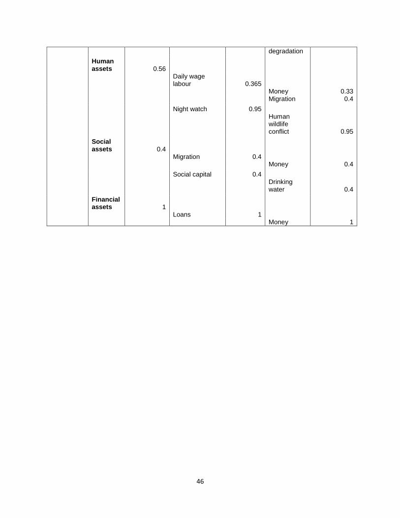
46

degradation

Human assets 0.56

Daily wage labour 0.365

Money 0.33

Migration 0.4

Night watch 0.95


Social assets 0.4

Migration 0.4

Money 0.4

Social capital 0.4

Drinking water 0.4

Financial assets 1

Loans 1

Money 1

pramod k. singh and abhishek nair - irma | home · 2013-09-02 · pramod k. singh and abhishek nair...

Documents