pr4 wacc for eirgrid and esb network - cru.ie · pdf fileintroduction and context - 2 - table...
TRANSCRIPT

[Type here]
- 1 -
PR4 WACC for EirGrid and
ESB Network
January 2015

Europe Economics is registered in England No. 3477100. Registered offices at Chancery House, 53-64 Chancery Lane, London WC2A 1QU.
Whilst every effort has been made to ensure the accuracy of the information/material contained in this report, Europe Economics assumes no
responsibility for and gives no guarantees, undertakings or warranties concerning the accuracy, completeness or up to date nature of the
information/analysis provided in the report and does not accept any liability whatsoever arising from any errors or omissions.
© Europe Economics. All rights reserved. Except for the quotation of short passages for the purpose of criticism or review, no part may be used or
reproduced without permission.

Contents
1 Introduction and Context ........................................................................................................................................... 1
1.1 Background ............................................................................................................................................................. 1
1.2 Overview of methodology .................................................................................................................................. 3
2 Risk-Free Rate ................................................................................................................................................................ 6
2.1 PR3, Mid-Term Review and stakeholder submissions ................................................................................. 6
2.2 Characteristics of a risk-free asset ................................................................................................................... 6
2.3 Methodological issues .......................................................................................................................................... 6
2.4 Regulatory precedent .......................................................................................................................................... 7
2.5 Developments ........................................................................................................................................................ 8
2.6 Conclusion .............................................................................................................................................................. 9
3 Debt Premium and Cost of Debt ............................................................................................................................ 11
3.1 Our approach to the estimation of the cost of debt ................................................................................. 11
3.2 Data sampling ....................................................................................................................................................... 14
3.3 Target credit rating: PR3 and stakeholder submissions ............................................................................ 14
3.4 Target credit rating: Our view ........................................................................................................................ 14
3.5 Debt premium: PR3, Mid-Term Review and stakeholder submissions .................................................. 16
3.6 Evidence from spreads of Irish energy company bonds ............................................................................ 16
3.7 Evidence from spreads of European comparator company bonds ......................................................... 17
3.8 Regulatory precedent ........................................................................................................................................ 24
3.9 Developments ...................................................................................................................................................... 24
3.10 Conclusion ............................................................................................................................................................ 24
4 Equity Risk Premium................................................................................................................................................... 26
4.1 PR3, Mid-Term Review and Sta ....................................................................................................................... 26
4.2 The Equity Risk Premium .................................................................................................................................. 26
4.3 Methodological issues ........................................................................................................................................ 27
4.4 Regulatory precedent ........................................................................................................................................ 29
4.5 Developments ...................................................................................................................................................... 30
4.6 Conclusion ............................................................................................................................................................ 31
5 Equity Beta and Cost of Equity ................................................................................................................................ 32
5.1 PR3, Mid-Term Review and Stakeholder Submissions regarding asset beta ........................................ 32
5.2 Analysis of risks faced by the TAO, DSO and TSO ................................................................................... 32
5.3 Methodology ........................................................................................................................................................ 36
5.4 Analysis of comparators .................................................................................................................................... 41
5.5 Regulatory precedent ........................................................................................................................................ 44
5.6 Companies’ submissions ................................................................................................................................... 45
5.7 Recent developments ........................................................................................................................................ 45

5.8 Conclusion ............................................................................................................................................................ 45
6 Capital Structure ......................................................................................................................................................... 46
6.1 PR3, Mid-Term Review and Stakeholder Submissions............................................................................... 46
6.2 Introduction ......................................................................................................................................................... 46
6.3 Capital structure and CAPM ............................................................................................................................ 46
6.4 Implications within a WACC framework ..................................................................................................... 49
6.5 Regulatory precedent ........................................................................................................................................ 50
6.6 Companies’ submissions ................................................................................................................................... 51
6.7 Conclusion ............................................................................................................................................................ 51
7 Taxes .............................................................................................................................................................................. 52
7.1 PR3, Mid-Term Review and stakeholder submissions ............................................................................... 52
7.2 Introduction ......................................................................................................................................................... 52
7.3 Different Options for the Treatment of Taxation ...................................................................................... 52
7.4 Treatment of tax benefits from gearing above notional level .................................................................. 53
7.5 Timing differences ............................................................................................................................................... 53
7.6 Companies’ submissions ................................................................................................................................... 54
7.7 Conclusions .......................................................................................................................................................... 54
8 WACC ........................................................................................................................................................................... 55
8.1 Summary ............................................................................................................................................................... 55
8.2 The principle of aiming up ................................................................................................................................ 55
8.3 Regulatory precedent ........................................................................................................................................ 57
8.4 Recommended WACC range and aimed-up point WACC ..................................................................... 58
8.5 Inflation .................................................................................................................................................................. 59
9 Financeability ................................................................................................................................................................ 60
9.1 Role of financeability .......................................................................................................................................... 60
9.2 ESB Financeability: indicative analysis ............................................................................................................ 60

Introduction and Context
- 1 -
1 Introduction and Context
The current report has been prepared by Europe Economics for the Commission for Energy Regulation
(CER) and sets out our views on the cost of capital for the Transmission System Operator (TSO) EirGrid
and ESB Networks (ESBN) which serves as both the Transmission Asset Owner (TAO) and Distribution
System Operator (DSO) and Distribution Asset Owner (DAO).
The role of the TSO in Ireland is to operate and maintain a safe, secure, reliable, economical and efficient
transmission system, as well as to plan and develop key infrastructural projects which are vital for the socio-
economic development of the State.1 As the DSO, ESBN builds, operates and maintains a nationwide
distribution system. ESBN also has the role of a TAO which is to “ensure that the Transmission System is
developed and maintained in accordance with the requirements set down by EirGrid”.2
We outline below relevant developments that took place in the years leading up to PR4, we briefly summarise
the methodological framework adopted, and we set out the structure of the remainder of the report.
1.1 Background
This section provides an outline of the developments that took place in the years leading up to PR4. We
first present a summary of the 2010 determination followed by a description of the Mid-Term WACC review
that was conducted in 2013 along with CER’s determination at the time.
1.1.1 The 2010 determination
Europe Economics advised the CER on the WACC during the last price review for electricity transmission
and distribution networks in Ireland (PR3). Based on market data up to the data cut-off point of February
2010, Europe Economics’ suggested a range estimate of the WACC (on a real pre-tax basis) of 3.2-5.6 per
cent and a point estimate (without aiming-up) of 4.6 per cent. The recommended regulatory WACC was
somewhat higher at 5.0 per cent, and drawn from a range of 4.8-5.2. This uplift was the result of a deliberately
“aiming up” to reflect the asymmetry of consequences for consumers if the WACC is set too low rather
than too high. The Europe Economics recommended estimates of each WACC component in PR3 are
summarised in the table below.
1 Source: http://www.EirGrid.com/aboutus/. 2 Source: http://www.esb.ie/esbnetworks/en/about-us/index.jsp.
Introduction and Context
- 2 -
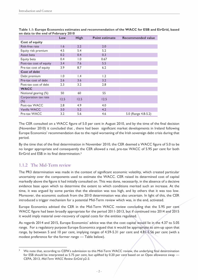
Table 1.1: Europe Economics estimates and recommendation of the WACC for ESB and EirGrid, based
on data to the end of February 2010
Low High Point estimate Recommended value
Cost of equity
Risk-free rate 1.6 2.2 2.0
Equity risk premium 4.5 5.4 5.2
Asset beta 0.2 0.4 0.3
Equity beta 0.4 1.0 0.67
Post-tax cost of equity 3.4 7.6 5.5
Pre-tax cost of equity 3.9 8.7 6.2
Cost of debt
Debt premium 1.0 1.4 1.2
Pre-tax cost of debt 2.6 3.6 3.2
Post-tax cost of debt 2.3 3.2 2.8
WACC
Notional gearing (%) 50 60 55
Corporation tax rate
(%) 12.5 12.5 12.5
Post-tax WACC 2.8 4.9 4.0
Vanilla WACC 3.0 5.2 4.2
Pre-tax WACC 3.2 5.6 4.6 5.0 (Range 4.8-5.2)
The CER consulted on a WACC figure of 5.0 per cent in August 2010, and by the time of the final decision
(November 2010) it concluded that , there had been significant market developments in Ireland following
Europe Economics’ recommendation due to the rapid worsening of the Irish sovereign debt crisis during that
period.
By the time that of the final determination in November 2010, the CER deemed a WACC figure of 5.0 to be
no longer appropriate and consequently the CER allowed a real, pre-tax WACC of 5.95 per cent for both
EirGrid and ESB in its final determination.3
1.1.2 The Mid-Term review
The PR3 determination was made in the context of significant economic volatility, which created particular
uncertainty over the components used to estimate the WACC. CER raised its determined cost of capital
markedly above the figure it had initially consulted on. This was done, necessarily, in the absence of a decisive
evidence base upon which to determine the extent to which conditions merited such an increase. At the
time, it was argued by some parties that the elevation was too high, and by others that it was too low.
Moreover, the economic outlook from the 2010 determination was also uncertain. In light of this, the CER
introduced a trigger mechanism for a potential Mid-Term review which was, in the end, activated.
Europe Economics advised the CER in the Mid-Term WACC review concluding that the 5.95 per cent
WACC figure had been broadly appropriate for the period 2011-2013, but if continued into 2014 and 2015
it would imply material over-recovery of capital costs for the entities regulated.
As regards 2014 and 2015, Europe Economics’ advice was that the cost capital would lie in the 4.37 to 5.05
range. For a regulatory purpose Europe Economics argued that it would be appropriate to aim-up upon that
range, by between 5 and 10 per cent, implying ranges of 4.59-5.31 per cent and 4.81-5.56 per cent (with a
modest preference for the former range — Table below).
3 We note that, according to CEPA’s submission to this Mid-Term WACC review, the underlying final determination
for ESB should be interpreted as 5.75 per cent, but uplifted by 0.20 per cent based on an Opex allowance swap —
CEPA, 2013, Mid-Term WACC Review EirGrid p2-3.
Introduction and Context
- 3 -
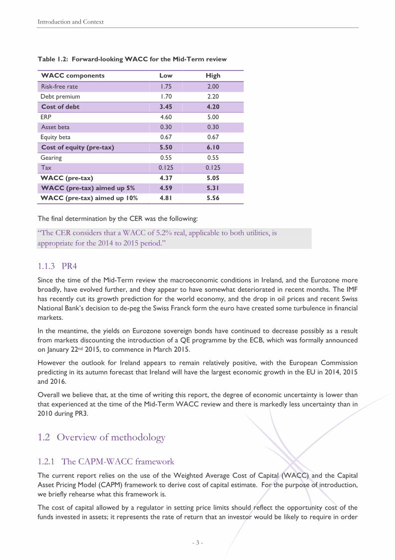
Table 1.2: Forward-looking WACC for the Mid-Term review
WACC components Low High
Risk-free rate 1.75 2.00
Debt premium 1.70 2.20
Cost of debt 3.45 4.20
ERP 4.60 5.00
Asset beta 0.30 0.30
Equity beta 0.67 0.67
Cost of equity (pre-tax) 5.50 6.10
Gearing 0.55 0.55
Tax 0.125 0.125
WACC (pre-tax) 4.37 5.05
WACC (pre-tax) aimed up 5% 4.59 5.31
WACC (pre-tax) aimed up 10% 4.81 5.56
The final determination by the CER was the following:
“The CER considers that a WACC of 5.2% real, applicable to both utilities, is
appropriate for the 2014 to 2015 period.”
1.1.3 PR4
Since the time of the Mid-Term review the macroeconomic conditions in Ireland, and the Eurozone more
broadly, have evolved further, and they appear to have somewhat deteriorated in recent months. The IMF
has recently cut its growth prediction for the world economy, and the drop in oil prices and recent Swiss
National Bank’s decision to de-peg the Swiss Franck form the euro have created some turbulence in financial
markets.
In the meantime, the yields on Eurozone sovereign bonds have continued to decrease possibly as a result
from markets discounting the introduction of a QE programme by the ECB, which was formally announced
on January 22nd 2015, to commence in March 2015.
However the outlook for Ireland appears to remain relatively positive, with the European Commission
predicting in its autumn forecast that Ireland will have the largest economic growth in the EU in 2014, 2015
and 2016.
Overall we believe that, at the time of writing this report, the degree of economic uncertainty is lower than
that experienced at the time of the Mid-Term WACC review and there is markedly less uncertainty than in
2010 during PR3.
1.2 Overview of methodology
1.2.1 The CAPM-WACC framework
The current report relies on the use of the Weighted Average Cost of Capital (WACC) and the Capital
Asset Pricing Model (CAPM) framework to derive cost of capital estimate. For the purpose of introduction,
we briefly rehearse what this framework is.
The cost of capital allowed by a regulator in setting price limits should reflect the opportunity cost of the
funds invested in assets; it represents the rate of return that an investor would be likely to require in order

Introduction and Context
- 4 -
to invest in a company, given its risk profile compared with other potential investments. It can also be thought
of as the discount rate which an investor would use in evaluating the income stream to be expected from
investing in the company.
The weighted average cost of capital (WACC) is computed from (a) the average cost of debt for the various
forms of debt held by the company, and (b) the cost of equity. This is the return that investors (shareholders
and lenders of various types) require in order to invest in the company.
Mathematically, the following formula is used:
[1]
where rE is the cost of equity, rD is the cost of debt, and E and D are the total values of equity and debt
respectively used to determine the level of gearing in the company, so giving the relative weights between
the cost of equity and debt finance.
Cost of debt
The cost of debt measures the combination of interest rates charged by banks to the company and the return
paid by the company on any corporate bonds or other loan instruments issued. It is standard practice to
think of this as being made up of a risk-free component and a company-specific risk premium.
𝑟𝑑 = 𝑟𝑓 + 𝑑𝑒𝑏𝑡 𝑝𝑟𝑒𝑚𝑖𝑢𝑚 [2]
rf is the return on a risk-free asset, usually proxied by a measure of the rate on medium to long-term
government bonds.
There are generally two main approaches for estimating the cost of debt.
Estimating the all-in cost of debt directly by analysing corporate bonds’ yields.
Estimating corporate bonds spread over the risk-free rate and expressing the cost of debt by its two
identifying components, i.e. risk-free rate plus debt premium.
For reasons we shall explain later, we prefer the second approach.
Cost of equity
The capital asset pricing model (CAPM) is used to determine the cost of equity, rE, applying the following
equation:
[3]
βE is the correlation between the risk in company returns and those of the market as a whole, which can
be estimated from primary market data for listed companies, or by analysing the betas of comparators
for companies which are not listed.
MRP is the market-risk premium over the risk-free rate, an Irish economy-wide parameter. Conceptually,
the market includes all assets. In practice, however, it is generally assumed that a broad equity market-
base index is a good proxy. Thus, estimates of the equity risk premium are used as a proxy in estimating
the MRP.
Thus in the standard CAPM there are three determinants of the expected return on any asset: the return
on a riskless asset - the market premium over that riskless rate that is earned by investors as a whole,
reflecting systematic risk; and the particular company’s exposure to systematic risk. As discussed further
below, company specific risks do not enter the cost of capital in the CAPM model, as they can, by definition,
be diversified away by investors.
ED
Dr
ED
ErWACC DE
.
MRPrr EfE *

Introduction and Context
- 5 -
Approach to risks
Under CAPM, risks are divided into two major categories:
systematic risks; and
specific risks.
Systematic risks are risks that affect the whole market. Systematic risks relate to outcomes that cause the
whole market to move, such as economic growth or recession, or wars. Even fully diversified investors are
subject to systematic risk, and require a compensation for it through the cost of capital. The amount of
compensation (the level of the cost of capital) they require from a particular company or a project depends
on how exposed that company is to systematic risks.
The specific risks affecting an individual firm are those risks that can be offset by investors diversifying their
investments. These are not taken into account in CAPM because it is assumed that in an efficient capital
market investors can protect themselves against such risks by holding a diversified portfolio. Thus, in CAPM,
specific risks are assumed not to affect the rate of return to investors (i.e. because they can be diversified
away) that the company has to cover through its cost of capital.
If you consider an industry in which there is no systematic risk (and no industry-specific risk), but each of the
companies in the industry faces company-specific risk CAPM predicts that the rate of return in this industry
would be the risk-free rate. Since there is no systematic risk, an investor with equal shares in all the
companies in the industry would be guaranteed to receive the risk-free rate every period — the company-
specific risks taken that turned out badly in some companies would exactly balance those that turned out
well in others (that is precisely what it means to say that there is no systematic risk).4
An example of a specific risk would be cost shocks caused by failure of the engineering solutions adopted by
an electricity network company.
1.2.2 Structure of the report
The report is organised in the following sections:
Risk-free rate
Debt premium and cost of debt
Equity risk premium
Equity beta and cost of equity
Capital structure
Taxes
WACC
4 Note that industry-wide industry-specific risks can be diversified by investors, in an analogous way to that set out in
the thought experiment above, through holding shares across industries.

Risk-Free Rate
- 6 -
2 Risk-Free Rate
2.1 PR3, Mid-Term Review and stakeholder submissions
In PR3 (2010) we recommended a risk–free rate range of 1.6-2.2 with a point estimate of 2.0. Our advice for
the Mid-Term WACC review (2013) was for a range of 1.75-2.0.
ESBN proposes a risk-free rate estimate of 2.0 per cent, based on Frontier’s analysis, and EirGrid, based on
KPMG’s analysis adopts a 1.75 per cent estimate, noting upward potential which would justify a 2.0 per cent
level.
2.2 Characteristics of a risk-free asset
By definition a risk-free asset is an asset that bears no risk (e.g. no credit or default risk, no currency risk, no
inflation risk and no reinvestment risk). Therefore the rate of return on a risk-free asset reflects, partially but
not exclusively, economic agents’ impatience, i.e. how much agents would rather have things today than
tomorrow. However, the risk-free rate is not simply the return any one individual would require to hold a
risk-free asset. Rather, it is the return that would be available in such an asset. As such, (a) it reflects
collective tastes, rather than those of any individual — the “taste” of the Market; and (b) it reflects an (albeit
notional) equilibrium condition. In standard long-term economic growth models, such as the Ramsey-Cass-
Koopmans model, a key equilibrium condition is that (absent population growth) the sustainable growth rate
of the economy is a function of the risk-free rate.5 Indeed, in corporate finance theory the risk-free rate of
return is sometimes viewed as arising from the sustainable growth rate (i.e. causality runs from the sustainable
growth rate to the risk-free rate).
2.3 Methodological issues
For PR4, we propose a single Eurozone risk-free rate figure, in line with the methodology we adopted for
the Mid-Term WACC review. As argued at the time of the mid-term WACC review, the use of a single
Eurozone risk-free rate reflects (a) the absence of currency exchange risk; (b) the high degree of capital
market integration within the Eurozone. As noted at the mid-term WACC review, this is a change from the
PR3 approach in which an Irish risk-free rate was estimated. This partly reflects the ongoing process of
capital market integration within the Eurozone but also reflects the fact that the data basis for estimating any
within-Eurozone variations in the risk-free rate (arising from residual segmentation of the Single Capital
Market) is weaker that was the case in 2010 — in recent years it has been very clear that Irish sovereign
bonds have not been treated as risk-free and there is no secure and robust basis for using any spreads
between Irish and other Eurozone sovereign bonds for estimating risk-free rate differentials as opposed to,
say, differences in perceived default risk or differences in the usefulness of such bonds as a speculative hedge
against euro disintegration. Candidates such as the use of sovereign credit default swaps prices have a number
of well-known weaknesses (e.g. low credibility — the Eurozone authorities went to great lengths, and in very
public ways, to try to design the Greek sovereign bonds default of 2012 such that it would not trigger CDS
payouts. Although, in the end, Greek sovereign CDS did pay out, the efforts to avoid such a payout are
widely acknowledged to have reduced the utility of sovereign CDS as a default hedge.).
5 Ramsey, F.P. (1928), "A mathematical theory of saving", Economic Journal, 38, 152, pp543–559. Cass, D. (1965),
“Optimum Growth in an Aggregative Model of Capital Accumulation”, Review of Economic Studies, 37 (3), pp233–240.
Risk-Free Rate
- 7 -
This has two implications:
Spreads (for the purpose of estimating risk asset premia (in particular debt premia with some implication,
also, for equity premia)) are estimated relative to the benchmark German government bond as selected
by Bloomberg.
The risk-free rate is determined based on Eurozone-wide macroeconomic considerations.
In the following sub-sections we present our thinking behind our recommended range and point estimate for
the risk-free rate that can be found in section 2.6.
2.3.1 Use of sovereign bonds
It is clear from the discussion above that, the risk–free asset is a theoretical concept rather than a particular
actual asset. For this reason, risk free-rate estimates are in practice carried out using the returns on assets
that are believed to constitute good proxies of riskless assets as a reference point. Government bonds have
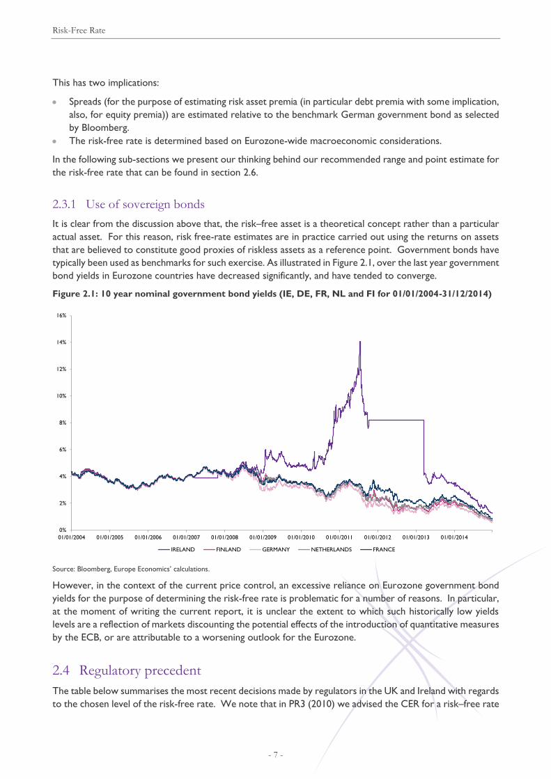
typically been used as benchmarks for such exercise. As illustrated in Figure 2.1, over the last year government
bond yields in Eurozone countries have decreased significantly, and have tended to converge.
Figure 2.1: 10 year nominal government bond yields (IE, DE, FR, NL and FI for 01/01/2004-31/12/2014)
Source: Bloomberg, Europe Economics’ calculations.
However, in the context of the current price control, an excessive reliance on Eurozone government bond
yields for the purpose of determining the risk-free rate is problematic for a number of reasons. In particular,
at the moment of writing the current report, it is unclear the extent to which such historically low yields
levels are a reflection of markets discounting the potential effects of the introduction of quantitative measures
by the ECB, or are attributable to a worsening outlook for the Eurozone.
2.4 Regulatory precedent
The table below summarises the most recent decisions made by regulators in the UK and Ireland with regards
to the chosen level of the risk-free rate. We note that in PR3 (2010) we advised the CER for a risk–free rate
0%
2%
4%
6%
8%
10%
12%
14%
16%
01/01/2004 01/01/2005 01/01/2006 01/01/2007 01/01/2008 01/01/2009 01/01/2010 01/01/2011 01/01/2012 01/01/2013 01/01/2014
IRELAND FINLAND GERMANY NETHERLANDS FRANCE

Risk-Free Rate
- 8 -
range of 1.6-2.2 with a point estimate of 2.0. Our advice for the Mid-Term WACC review (2013) was for a
range of 1.75-2.0.
Table 2.1: Recent regulatory precedent for the risk-free rate in the UK and Ireland
Company Ofwat
(2014)
CER
Irish
Water
(2014)
ComReg
Eircom
(2014)
CAR
DAA
(2014)
CC
NIE
(2013)
CRE
France
(2013)*
Bundesnetzagentur
Germany
(2013)*
Ofgem
NGET
(2012)
Risk-free
rate 1.25% 2.00% 2.10% 1.50% 1.50% 4.00% 3.80% 2.00%
*Note: Obtained from an Ernst & Young 2013 report:
http://www.ey.com/Publication/vwLUAssets/Mapping_power_and_utilities_regulation_in_Europe/$FILE/Mapping_power_and_utilities_regulation_in
_Europe_DX0181.pdf.
Our 2010 advice to the CER relied primarily on the yields of German and French government bonds, and on
Irish government bonds after adjustment using CDS data. It also took into account regulatory precedents,
and the tendency for regulators to estimate the risk-free rate to be slightly higher than real yields on
government bonds (which is why the bottom of our range was not extended to encompass all of the market
data we presented).
For the reasons set out above, in the context of the Mid-Term review and for PR4, our methodological
recommendation was to use a Eurozone-wide risk free rate. Based on the average real yields of 10-year
German bonds for the periods 2000-2013 and 2000-2007 and UK regulatory precedent for 2011-2012 (1.4
to 2 per cent) we determined that a range of 1.4-2.0 per cent was appropriate for 2011-2013 with a forward
looking rate of 1.75-2.0 per cent.
2.5 Developments
Government bond yields for Eurozone countries were decreasing throughout 2014 and have decreased more
since October 2014. We note that the observed levels may be distorted downwards. For example, as well
as the general deterioration in the macroeconomic outlook for the Eurozone (which might induce a genuine
reduction in the risk-free rate) playing an important role in this downward movement, the potential and
subsequent actual introduction of quantitative easing measures by the ECB may also be a factor (creating a
downwards distortion).
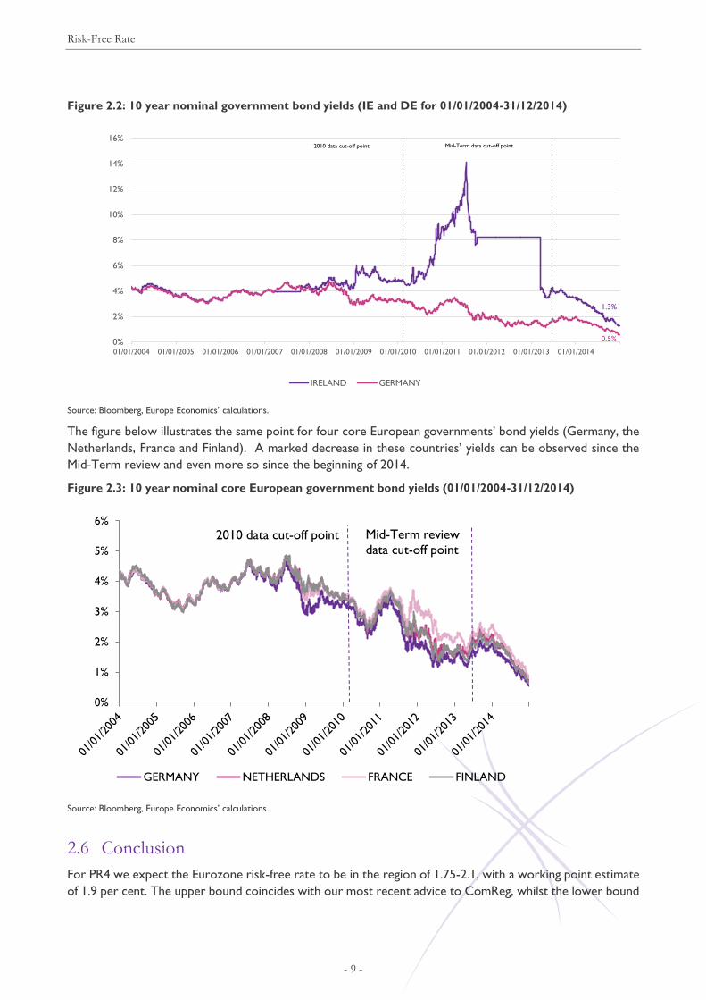
Figure 2.2 illustrates the movements of 10-year German and Irish government bond yields for the past 10
years. The convergence of Irish yields to Eurozone norm is becoming more evident from the decreased
difference of German and Irish yields. Both countries’ yields have been falling since July 2013 and reached a
spot level (as of 31/12/2014) of 1.3 per cent for Ireland and 0.5 per cent for Germany.
Risk-Free Rate
- 9 -
Figure 2.2: 10 year nominal government bond yields (IE and DE for 01/01/2004-31/12/2014)
Source: Bloomberg, Europe Economics’ calculations.
The figure below illustrates the same point for four core European governments’ bond yields (Germany, the
Netherlands, France and Finland). A marked decrease in these countries’ yields can be observed since the
Mid-Term review and even more so since the beginning of 2014.
Figure 2.3: 10 year nominal core European government bond yields (01/01/2004-31/12/2014)
Source: Bloomberg, Europe Economics’ calculations.
2.6 Conclusion
For PR4 we expect the Eurozone risk-free rate to be in the region of 1.75-2.1, with a working point estimate
of 1.9 per cent. The upper bound coincides with our most recent advice to ComReg, whilst the lower bound
0%
2%
4%
6%
8%
10%
12%
14%
16%
01/01/2004 01/01/2005 01/01/2006 01/01/2007 01/01/2008 01/01/2009 01/01/2010 01/01/2011 01/01/2012 01/01/2013 01/01/2014
IRELAND GERMANY
1.3%
0.5%
Mid-Term data cut-off point2010 data cut-off point
0%
1%
2%
3%
4%
5%
6%
GERMANY NETHERLANDS FRANCE FINLAND
2010 data cut-off point Mid-Term review
data cut-off point

Risk-Free Rate
- 10 -
reflects the potential for QE and deterioration in the Eurozone’s macroeconomic outlook and is also close
to the 2000-2014 average yield of German 10-year bonds.
We note that the forwards-looking mid-term WACC review figure was 1.75 to 2 for 2014-2015. That was
based upon the rate normalising to above 2 from late 2015 onwards, which would have implied that the late
2015-on range consistent with the mid-term WACC review would have been higher than 1.75 to 2. That
means that our 1.75-2.1 should be understood as involving a reduction in the risk-free rate range for late
2015-on implied by the mid-term WACC review range, reflecting the darkening of the macroeconomic
outlook since that time.

Debt Premium and Cost of Debt
- 11 -
3 Debt Premium and Cost of Debt
3.1 Our approach to the estimation of the cost of debt
3.1.1 Debt premium approach
There are generally two main approaches for estimating the cost of debt.
Estimating the all-in cost of debt directly by analysing corporate bonds’ yields.
Estimating corporate bonds spread over the risk-free rate and expressing the cost of debt by its two
identifying components, i.e. risk-free rate plus debt premium.
In estimating the cost of debt, we have adopted the approach of building up the cost of debt by summing the
risk-free rate (i.e. the return required by investors for investing in risk-free assets) and a company-specific
debt premium. This approach will ensure consistency with the way in which the cost of equity is calculated,
since the same risk-free rate assumption is being used.
Additionally, in a CAPM framework, there are conceptual differences between the movements in the debt
premium and movements in the risk-free rate. Changes in the debt premium may occur due to re-evaluations
of risk or changes in risk appetite for the company in question, which are distinct from the changes captured
by risk-free rate variations. Separating the components of the cost of debt therefore allows for a more
focused analysis of the cost of debt.
Second, with a debt premium approach, forward-looking estimates of a rise in the risk-free rate convert
straightforwardly into a forward-looking cost of debt estimate. In the approach that uses the overall cost of
debt this relationship is unclear. For example, loose monetary policy and quantitative easing are intended to
reduce market interest rates below the cost of debt in order to enhance incentives to invest. The effect of
this policy on market rates has been discussed in our analysis of the risk-free rate. An overall cost of debt
approach risks under-appreciating the effects of deliberate policies upon debt costs.
Putting the point a different way, our approach to the risk-free rate can be seen as envisaging a certain
scenario for the equilibrium level of sovereign bond yields. The use of a debt premium approach means that
the scenarios for the equilibrium overall cost of debt involve the same rises in the cost of debt as those for
the risk-free rate, if the debt premium is fairly constant (as theory and empirical evidence suggest it will be).6
We also note that our estimated risk-free rate is itself generated in part from a disaggregation of total market
returns in their respective components. Given the advantages of a bottom-up approach to the forward-
looking cost of debt, we therefore prefer this approach to direct estimation from bond yields.
6 We note that in cases where an overall cost of debt is used, some assumption is required regarding how the overall
cost of debt will change as government bond yields are expected to change (e.g. as implied by futures markets). In the
debt premium approach the change is one for one. In its analysis of the overall cost of debt for the UK CAA as part of
the Q6 price review, PWC found the relationship was 0.8 for one, i.e. a rise of 1 per cent in government bond yields
implied a 0.8 per cent risk in the overall cost of debt. PWC does not report whether its statistical analysis suggests this
0.8 figure was statistically significantly different from 1, but we note that it rose from 0.6 to 0.8 between the interim and
final reports, which suggests a range of uncertainty of at least 0.2 is plausible – see:
http://www.caa.co.uk/docs/78/PwC_CAA_CostofCapital_Designated_Airports_Oct.pdf
Our view is that the use of a conversion coefficient so close to one (and potentially not statistically significantly different
from 1) makes the distinction between a debt premium approach and an overall cost of debt approach rather limited in
scope.

Debt Premium and Cost of Debt
- 12 -
EirGrid does not have any listed euro bonds while ESB only has three outstanding euro bonds maturing in
September 2017 (€600m), November 2019 (€500m) and January 2024 (€300m). There are also three
sterling-denominated ESB bonds maturing in 2018 (£175m), 2020 (£275m) and 2026 (£400m). In addition,
we note that there is also one outstanding Bord Gáis bond with less than three years to maturity that we
consider in our analysis and present along with the ESB bonds.7 Since there were only four Irish euro-
denominated bonds available, on top of examining ESB’s bonds, we informed our analysis of the debt premium
for ESB Networks and EirGrid with data on spreads of European comparator companies (i.e. other electricity
suppliers and utilities), and evidence from regulatory precedent. In order to ensure consistency, we have
only used comparator companies that were used either in PR3 or the Mid-Term review (or both).8
When considering relevant comparator bonds it is more appropriate to rely on bonds in the same credit
class as opposed to focusing on bonds across classes that have the same credit rating. This is partly because
of the conceptual difference between the market debt premium (MDP) (i.e. the spread of bond yields over the
benchmark observable from market data) and the expected return from holding debt — the relevant concept
in the CAPM framework — which reflects inventors’ expected returns on debt after taking into account the
probability of default and the loss given default. Within the CAPM framework the probability of default and
loss given default are relevant only to the extent to which they reflect systematic risks that cannot be
diversified (e.g. defaults and losses that are correlated with the broader market). However, credit ratings
reflect also idiosyncratic risks and therefore, for the purpose of estimating debt premium, credit ratings on
bonds in different credit classes (e.g. financials as versus transport as versus utilities) should be regarded as
only imprecise measures of systematic risk. When bonds of the same rating within the same credit class (e.g.
utilities) are used, there is a much better chance that the debt premium reflects a fairly consistent ratio of
systematic to idiosyncratic risk.
3.1.2 Use of embedded debt
An embedded debt approach involves combining estimates of companies’ existing costs of debt with an
estimate of their forward-looking cost of debt, and weighting these according to the companies’ expected
future debt requirements. A forward-looking cost of debt approach does not take into account embedded
debt costs, and instead relies on estimating what would be the costs of debt for new issuances.
An embedded debt approach may be appropriate for pragmatic reasons. For example, there may be feasibility
problems for existing companies in adjusting costs quickly to an efficient level or it may have been cheaper
to acquire or build relevant assets in the past than is currently the case. This approach may also be used by
regulators seeking to meet duty-to-finance obligations. None of these cases would necessarily require a
regulator to make an embedded debt adjustment, but such an approach may represent an appropriate
pragmatic response to particular circumstances.
However, in the absence of such considerations, it is preferable not to apply embedded debt adjustments.
This is because the key thought experiment in a price control is that of the competitive or contestable market,
the existence of the control being due to a lack of competitive constraint. An efficient new entrant would
not have access to past debts obtained at rates cheaper than those at the time of entry, nor would it have
legacy debt that was more expensive than the debt it could obtain at entry. An efficient new entrant would
7 We note that Bord Gáis Éireann was renamed Ervia in 2014 and that its energy part was sold to Centrica in
December 2013. 8 In the stakeholder submissions, ESB’s consultants Frontier use only ESBN’s own bonds. EirGrid’s consultants KPMG
use a range of bonds including a EuroGrid bond (2020), an RTE bond (2022), an Elia bond (2028) and a Fingrid bond
(2028), plus a set of UK National Grid bonds ranging in maturity dates from 2017 to 2028. RTE is a subsidiary of EDF.
We have considered National Grid and EDF bonds where they satisfied our data sampling criteria, which in practice
excludes the National Grid bonds KPMG quotes but EDF bonds from 2022-2026 are included in our analysis below.

Debt Premium and Cost of Debt
- 13 -
therefore neither gain nor suffer due to embedded debt.9 Thus, although pragmatic considerations may justify
the use of embedded debt under some circumstances, best practice in economic regulation should be to seek
to phase out embedded debt adjustments as and when doing so becomes feasible.10We observe that the
CER’s 2012 BGN decision included an allowance for embedded debt, presumably reflecting the exceptional
circumstances of that very turbulent period. We do not believe that this should be regarded as establishing
any precedent for the treatment of embedded debt in more stable market conditions.
Our approach for determining the cost of debt is therefore to estimate a forward-looking cost of debt and
make no embedded debt adjustment.
3.1.3 Use of indexation
Some regulators (e.g. Ofgem in the UK, or CER for BGN in 2012 — though the BGN indexation method is
very different from Ofgem’s) have adopted an approach to the cost of debt wherein the cost of debt
allowance in the price control is indexed, in a manner somewhat akin to the indexation of prices with respect
to inflation.
Four main kinds of rationale are offered in defence of indexation:
a) Movements in the risk-free rate are economy-wide and, as such, would affect all firms and hence feed
through into prices in a competitive market.
b) Insofar as risk-free rates are estimated directly from government bond rates, they are a reflection of
macroeconomic policy measures (e.g. central bank interest rates or QE) that would affect all firms equally
and as such closely analogous to (indeed, affected by the same factors as) inflation.
c) In an era of low and falling government bond yields, regulators have been cautious about reducing risk-
free rate determinations in line with sovereign yield falls, perhaps fearing a reversion of yields to historic
norms over the period of price controls. This has resulted in a tendency for risk-free rate determinations
to include “headroom” over sovereign bond yields as a form of insurance against sudden rises in those
yields. Indexation provides an alternative insurance policy, allowing regulators to set risk-free rates more
closely in line with sovereign bond yields.
d) In the case of BGN, conditions were so extreme and uncertainty so high that, absent some mechanism
for indexation, it would very probably have been necessary to re-open the WACC in particular or even
the price control in general mid-way through the control period. Indexation was thus an alternative to
a mid-term review (the approach taken by the CER in the case of electricity transmission and distribution
for PR3).
In the current context, since we are not estimating risk-free rates directly from sovereign bond yields,
argument (b) is straightforwardly inapplicable. Regarding argument (c) we do not regard our judgement as
involving headroom11 as such — there is no implicit forecast for bond yields or insurance against adverse
movements in such yields in our recommendation. We regard this as more of an issue for regulators that
have had a tradition of providing such headroom (e.g. Ofgem). As regards argument (d) we believe it is clear
that current macroeconomic conditions are not remotely as turbulent as those of 2012.
As regards argument (a) we consider it unconvincing in itself and unconvincing as a rationale for the use of
indexation. Firms have the scope to raise debt at various points over the price control period, and
investments have an extended life. As such, it is a mistake to believe that final prices for products will
9 These considerations do not make any presuppositions on the market share of either an entrant or existent market
participants. 10 ESBN bonds were issued in 2010 and one each year in 2011-2013. That was a period of elevated debt premia, which
were reflected in the WACC determinations at PR3 and in the mid-term WACC review. 11 We understand the term “headroom” in this context as referring to the determination of a value above one’s best
estimate of a WACC component to insure against an adverse movement over the price control period.

Debt Premium and Cost of Debt
- 14 -
generally move in line with the point risk-free rate. Instead, they are more likely to be correlated with
expected movements in the long-term risk-free rate, but even there, there is a question of which is cause
and which effect — higher growth might mean higher profits and higher prices, so raising risk-free rates,
rather than the reverse. But even if whole-economy prices were to move in line with risk-free rates, we
would regard efficient financing as part of the incentive structure of periodic-review-based regulation. Firms
manage risks, including the risk of adverse movements in the risk-free rate, over the period of the price
control.
To conclude, we therefore recommend against the use of indexation.
3.2 Data sampling
As mentioned above, our preferred methodology for estimating the debt premium consists of observing the
spread of corporate debt costs over the risk-free rate and not incorporating any embedded debt costs, as a
hypothetical efficient firm would manage its treasury operations to achieve the lowest cost of debt possible.
For estimation purpose the debt premium is calculated as the spread between the yields of risky assets
(corporate bonds) against the yields of 10-year German government bonds (i.e. a benchmark asset which is
perceived as having very low risk), noting that the purpose is to identify the spread from risk.12
The following two sections present an analysis of outstanding bonds issued by Irish and selected European
utilities. The criterial used for selection are as follows:
All the bonds selected have a “comfortable investment grade” (i.e. they are rated above BBB- from S&P
and Baa3 from Moody’s).
All bonds are denominated in euro (with the exception of UK utilities bonds which are denominated in
GBP).
For all bonds the spreads are calculated against an appropriate benchmark selected by Bloomberg. For
European utilities Bloomberg selected benchmarks are German government bonds, and for UK bonds
the selected benchmarks are UK Gilts.
All bonds have a time to maturity ranging between 8 and 12 years (when rounded).
3.3 Target credit rating: PR3 and stakeholder submissions
At PR3 the target credit ratings were in the A grade for both ESBN and Eirgrid.
For PR4 ESBN has proposed a credit rating of A-. EirGrid has proposed A.
3.4 Target credit rating: Our view
In estimating the cost of debt, one of the key methodological choices concerns the credit rating which should
be assumed for ESB Networks and EirGrid. When estimating the cost of debt for the 2001-2005 price
control period, the CER assumed that ESB Networks would maintain an A credit rating over the regulatory
period (which was deemed consistent with a notional assumed gearing of 50 per cent). In its 2006 price
control review, on the other hand, the CER assumed a credit rating of A or BBB for the price control period
(which was deemed to be consistent with a notional assumed level of gearing of 50-60 per cent). However,
in its response to a questionnaire sent by CER, ESB Networks stated that it did not have a formal target
rating.
12 The assumption upon which this method is based is that whatever factors downwards-distort government bonds
also downwards-distort yields on riskier assets.
Debt Premium and Cost of Debt
- 15 -
In contrast, no reference was made in either of these price reviews to the target credit rating for EirGrid
and according to its response to a questionnaire sent out by the CER, EirGrid also does not have a formal
target rating.
Our working assumption for estimating the cost of debt for the 2010 and the Mid-Term review, was that
ESB Networks and EirGrid would be able to issue bonds with a rating between BBB and A. This was in line
with regulatory practice since regulatory decisions (e.g. ComReg in November 2014) tend to regard a
comfortable investment grade rating (BBB+ or above), as being sufficient for utility companies to finance their
activities. However, we also note that significant changes in market environments may lead to revisions in
the target credit rating. For example, in 2009 we advised Ofwat carry out its financeability analysis for both
a target rating of A- and of BBB+. This decision was driven by the worsening of credit market condition at
that time and was supported by the following market evidence:
A significant increase in the yields on corporate bonds across all credit ratings (relative to 2007 values).
A widening of the wedge between yields on BBB rated bonds and bonds with superior ratings (relative
to 2007).
Mixed views expressed by investors as to whether a credit rating of BBB+ was sufficient for water
companies to access sufficient debt finance in the market at that turbulent time.
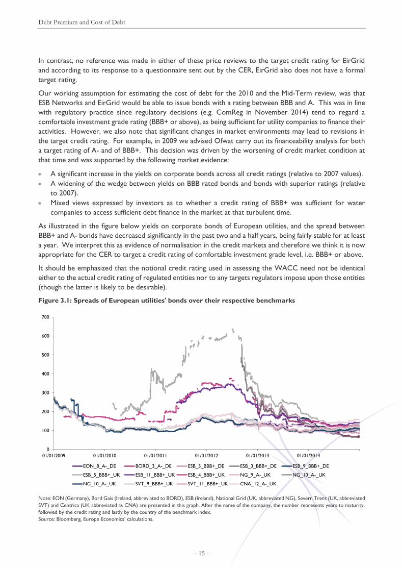
As illustrated in the figure below yields on corporate bonds of European utilities, and the spread between
BBB+ and A- bonds have decreased significantly in the past two and a half years, being fairly stable for at least
a year. We interpret this as evidence of normalisation in the credit markets and therefore we think it is now
appropriate for the CER to target a credit rating of comfortable investment grade level, i.e. BBB+ or above.
It should be emphasized that the notional credit rating used in assessing the WACC need not be identical
either to the actual credit rating of regulated entities nor to any targets regulators impose upon those entities
(though the latter is likely to be desirable).
Figure 3.1: Spreads of European utilities' bonds over their respective benchmarks
Note: EON (Germany), Bord Gais (Ireland, abbreviated to BORD), ESB (Ireland), National Grid (UK, abbreviated NG), Severn Trent (UK, abbreviated
SVT) and Centrica (UK abbreviated as CNA) are presented in this graph. After the name of the company, the number represents years to maturity,
followed by the credit rating and lastly by the country of the benchmark index.
Source: Bloomberg, Europe Economics’ calculations.
0
100
200
300
400
500
600
700
01/01/2009 01/01/2010 01/01/2011 01/01/2012 01/01/2013 01/01/2014
EON_8_A-_DE BORD_3_A-_DE ESB_5_BBB+_DE ESB_3_BBB+_DE ESB_9_BBB+_DE
ESB_5_BBB+_UK ESB_11_BBB+_UK ESB_4_BBB+_UK NG_9_A-_UK NG_10_A-_UK
NG_10_A-_UK SVT_9_BBB+_UK SVT_11_BBB+_UK CNA_12_A-_UK

Debt Premium and Cost of Debt
- 16 -
3.5 Debt premium: PR3, Mid-Term Review and stakeholder submissions
At PR3 we recommended a debt premium range of 1.0 to 1.4 with a point estimate of 1.2. At the mid-term
review the range was 1.7-2.2.
At PR4, ESBN’s point estimate for the debt premium is 1.75 per cent, as is EirGrid’s when including “issuance”
and “access to finance” uplifts of 25 bps (with a range of 1.5-2.0 per cent).
3.6 Evidence from spreads of Irish energy company bonds
Figure 3.2 illustrates how the spreads of euro denominated Irish energy bonds have steadily decreased since
the cut-off date of the Mid-Term review (16/07/2013). A snapshot of this information is also presented in
Table 3.1 where we observe spot rates for ESB bonds ranging from 64 (three years to maturity) up to 100
bps (9 years to maturity). These values are significantly lower than their respective one year averages,
reflecting the downward trajectory that the spreads have followed.
Figure 3.2: Spread of euro denominated Irish utilities’ bonds (bps) over the German benchmark bond
Numbers in the legend represent years to maturity, followed by credit rating and the country of the benchmark bond used.
Source: Bloomberg, Europe Economics’ calculations.
0
50
100
150
200
250
300
350
400
450
500
06/09/2012 06/12/2012 06/03/2013 06/06/2013 06/09/2013 06/12/2013 06/03/2014 06/06/2014 06/09/2014 06/12/2014
BORD_3_A-_DE ESB_5_BBB+_DE ESB_3_BBB+_DE ESB_9_BBB+_DE
Mid-Term data cut-off point

Debt Premium and Cost of Debt
- 17 -
Table 3.1: Spread of euro denominated Irish utilities’ bond over the German benchmark bond (in bps,
as of 31/12/2014)
Company Sector Years to
Maturity
Rating
(S&P)
Spread
31/12/2014
Average
(1 year)
Max
(1 year)
Min
(1 year)
BORD GAIS Gas 3 A- 70 95 142 66
ESB Electricity 3 BBB+ 64 94 151 63
ESB Electricity 5 BBB+ 86 114 166 86
ESB Electricity 9 BBB+ 100 120 167 97
Average 80 106 156 78
Average ESB 83 109 161 82 Note: Years to maturity are rounded figures. Averages are raw.
Source: Bloomberg, EE calculations.
For completeness in the table below we present also the spreads of outstanding sterling denominated ESB.
We note that the spot spreads range from 121 (four years to maturity) to 140 (eleven years to maturity) and
that the bonds with shorter time to maturity are currently trading at below their one year average spreads.
Table 3.2: Spread of sterling denominated ESB bond over UK gilts (in bps, as of 31/12/2014)
Company Sector Years to
Maturity
Rating
(S&P)
Spread
31/12/2014
Average
(1 year)
Max
(1 year)
Min
(1 year)
ESB Electricity 4 BBB+ 121 131 157 119
ESB Electricity 5 BBB+ 129 138 184 119
ESB Electricity 11 BBB+ 140 137 152 124
Average 130 135 164 121 Note: Years to maturity are rounded figures.
Source: Bloomberg, EE calculations.
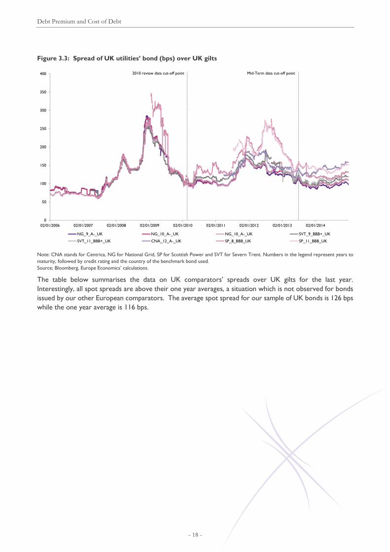
3.7 Evidence from spreads of European comparator company bonds
Below we provide figures presenting the spreads of a number of European utilities. While the spreads
exhibited considerable volatility since the 2010 review and less so since the Mid-Term review, visual
inspection shows that they have not moved markedlyin any direction, in the past year.
Debt Premium and Cost of Debt
- 18 -
Figure 3.3: Spread of UK utilities’ bond (bps) over UK gilts
Note: CNA stands for Centrica, NG for National Grid, SP for Scottish Power and SVT for Severn Trent. Numbers in the legend represent years to
maturity, followed by credit rating and the country of the benchmark bond used.
Source; Bloomberg, Europe Economics’ calculations.
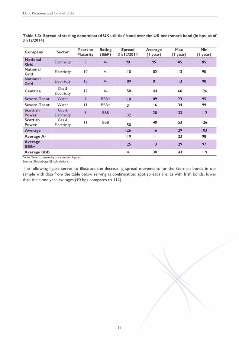
The table below summarises the data on UK comparators’ spreads over UK gilts for the last year.
Interestingly, all spot spreads are above their one year averages, a situation which is not observed for bonds
issued by our other European comparators. The average spot spread for our sample of UK bonds is 126 bps
while the one year average is 116 bps.
0
50
100
150
200
250
300
350
400
02/01/2006 02/01/2007 02/01/2008 02/01/2009 02/01/2010 02/01/2011 02/01/2012 02/01/2013 02/01/2014
NG_9_A-_UK NG_10_A-_UK NG_10_A-_UK SVT_9_BBB+_UK
SVT_11_BBB+_UK CNA_12_A-_UK SP_8_BBB_UK SP_11_BBB_UK
Mid-Term data cut-off point2010 review data cut-off point
Debt Premium and Cost of Debt
- 19 -
Table 3.3: Spread of sterling denominated UK utilities’ bond over the UK benchmark bond (in bps, as of
31/12/2014)
Company Sector Years to
Maturity
Rating
(S&P)
Spread
31/12/2014
Average
(1 year)
Max
(1 year)
Min
(1 year)
National
Grid Electricity 9 A- 98 95 105 85
National
Grid Electricity 10 A- 110 102 113 90
National
Grid Electricity 10 A- 109 101 113 90
Centrica Gas &
Electricity 12 A- 158 144 160 126
Severn Trent Water 9 BBB+ 119 109 123 95
Severn Trent Water 11 BBB+ 131 116 134 99
Scottish
Power
Gas &
Electricity 8 BBB
132 120 133 112
Scottish
Power
Gas &
Electricity 11 BBB
150 140 153 126
Average 126 116 129 103
Average A- 119 111 123 98
Average
BBB+ 125 113 129 97
Average BBB 141 130 143 119
Note: Years to maturity are rounded figures.
Source: Bloomberg, EE calculations.
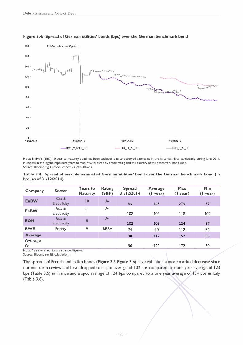
The following figure serves to illustrate the decreasing spread movements for the German bonds in our
sample with data from the table below serving as confirmation; spot spreads are, as with Irish bonds, lower
than their one year averages (90 bps compares to 112).
Debt Premium and Cost of Debt
- 20 -
Figure 3.4: Spread of German utilities’ bonds (bps) over the German benchmark bond
Note: EnBW’s (EBK) 10 year to maturity bond has been excluded due to observed anomalies in the historical data, particularly during June 2014.
Numbers in the legend represent years to maturity, followed by credit rating and the country of the benchmark bond used.
Source: Bloomberg, Europe Economics’ calculations.
Table 3.4: Spread of euro denominated German utilities’ bond over the German benchmark bond (in
bps, as of 31/12/2014)
Company Sector Years to
Maturity
Rating
(S&P)
Spread
31/12/2014
Average
(1 year)
Max
(1 year)
Min
(1 year)
EnBW Gas &
Electricity 10 A-
83 148 273 77
EnBW Gas &
Electricity 11
A-
102 109 118 102
EON Gas &
Electricity 8
A-
102 103 124 87
RWE Energy 9 BBB+ 74 90 112 74
Average 90 112 157 85 Average
A-
96 120 172 89 Note: Years to maturity are rounded figures.
Source: Bloomberg, EE calculations.
The spreads of French and Italian bonds (Figure 3.5-Figure 3.6) have exhibited a more marked decrease since
our mid-term review and have dropped to a spot average of 102 bps compared to a one year average of 123
bps (Table 3.5) in France and a spot average of 124 bps compared to a one year average of 134 bps in Italy
(Table 3.6).
0
20
40
60
80
100
120
140
160
180
25/01/2013 25/07/2013 25/01/2014 25/07/2014
RWE_9_BBB+_DE EBK_11_A-_DE EON_8_A-_DE
Mid-Term data cut-off point

Debt Premium and Cost of Debt
- 21 -
Figure 3.5: Spread of French utilities’ bonds (bps) over the German benchmark bond
Note: Numbers in the legend represent years to maturity, followed by credit rating and the country of the benchmark bond used.
Source: Bloomberg, Europe Economics’ calculations.
Table 3.5: Spread of euro denominated French utilities’ bond over the German benchmark bond (in bps,
as of 31/12/2014)
Company Sector Years to
Maturity
Rating
(S&P)
Spread
31/12/2014
Average
(1 year)
Max
(1 year)
Min
(1 year)
EDF Energy 8 A+ 74 92 112 73
EDF Energy 10 A+ 136 172 204 136
EDF Energy 11 A+ 145 170 189 145
GDF Gas &
Electricity 8
A 61 79 93 61
GDF Gas &
Electricity 11 A 92 100 107 92
Average 102 123 141 101
Average
A+ 118 145 168 118
Average
A 77 90 100 76
Note: Years to maturity are rounded figures.
Source: Bloomberg, EE calculations.
0
50
100
150
200
250
300
07/09/2009 07/09/2010 07/09/2011 07/09/2012 07/09/2013 07/09/2014
GDF_8_A_DE GDF_11_A_DE EDF_8_A+_DE EDF_10_A+_DE EDF_11_A+_DE
Mid-Term data cut-off point2010 review data cut-off point

Debt Premium and Cost of Debt
- 22 -
Figure 3.6: Spread of Italian utilities’ bond (bps) over the German benchmark bond
Note: SRG stands for Snam Rete Gas. Numbers in the legend represent years to maturity, followed by credit rating and the country of the benchmark
bond used.
Source; Bloomberg, EE calculations.
Table 3.6: Spread of euro denominated Italian utilities’ bond over the German benchmark bond (in bps,
as of 31/12/2014)
Company Sector Years to
Maturity
Rating
(S&P)
Spread
31/12/2014
Average
(1 year)
Max
(1 year)
Min
(1 year)
ENEL Energy 8 BBB 118 135 196 109
ENEL Energy 9 BBB 121 145 222 111
ENEL Energy 9 BBB 109 125 206 94
ENEL Energy 10 BBB 142 150 209 132
A2A Electricity 9 BBB 156 153 197 139
Hera Gas &
Electricity 8 BBB 155 131 170 112
Hera Gas &
Electricity 9 BBB 104 108 115 102
Hera Gas &
Electricity 10 BBB 172 170 204 152
Terna Electricity 10 BBB 85 156 316 71
Snam
Rete Gas
Gas &
Electricity 8 BBB 102 92 109 81
Snam
Rete Gas
Gas &
Electricity 9 BBB 104 108 154 91
Average 124 134 191 109 Note: Years to maturity are rounded figures.
Source: Bloomberg, EE calculations.
Spanish utilities’ bonds that made our sample were issued in 2014 and hence do not have sufficient historical
data for the calculation of one year averages (see Figure 3.7). As a cross-check to other countries, we note
that their average spot spread is 96 (Table 3.7).
0
100
200
300
400
500
600
700
02/01/2006 02/01/2007 02/01/2008 02/01/2009 02/01/2010 02/01/2011 02/01/2012 02/01/2013 02/01/2014
ENEL_8_BBB_DE ENEL_9_BBB_DE ENEL_9_BBB_DE ENEL_10_BBB_DEA2A_9_Baa3_DE HERA_8_BBB_DE HERA_9_BBB_DE HERA_10_BBB_DETRN_9_BBB_DE TRN_10_BBB_DE SRG_8_BBB_DE SRG_9_BBB_DE
Mid-Term data cut-off point2010 review data cut-off point
Debt Premium and Cost of Debt
- 23 -
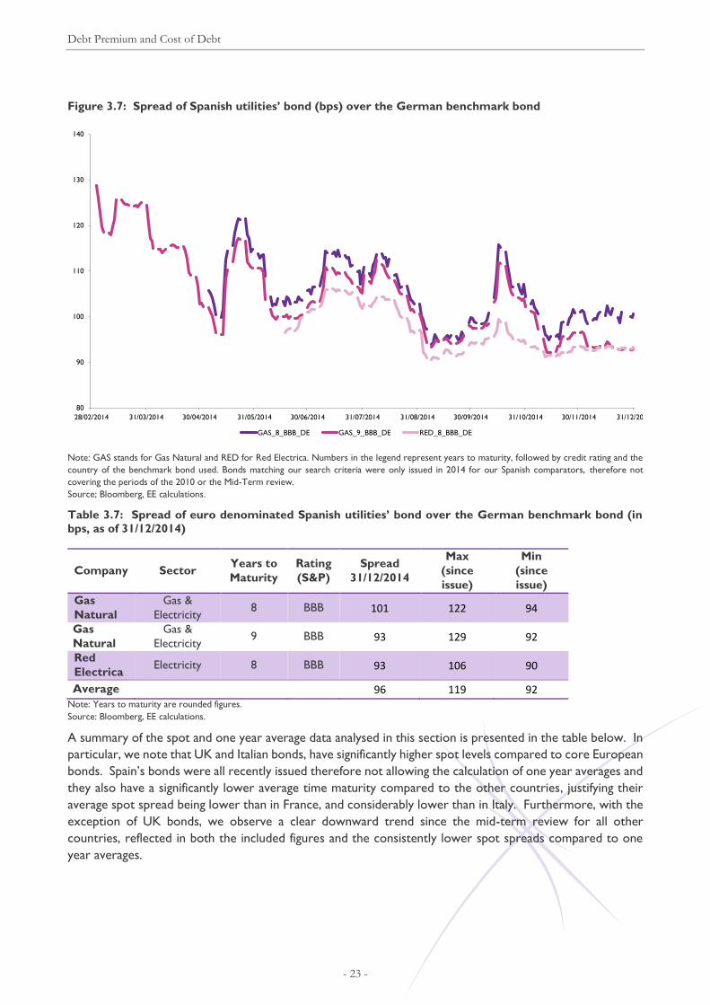
Figure 3.7: Spread of Spanish utilities’ bond (bps) over the German benchmark bond
Note: GAS stands for Gas Natural and RED for Red Electrica. Numbers in the legend represent years to maturity, followed by credit rating and the
country of the benchmark bond used. Bonds matching our search criteria were only issued in 2014 for our Spanish comparators, therefore not
covering the periods of the 2010 or the Mid-Term review.
Source; Bloomberg, EE calculations.
Table 3.7: Spread of euro denominated Spanish utilities’ bond over the German benchmark bond (in
bps, as of 31/12/2014)
Company Sector Years to
Maturity
Rating
(S&P)
Spread
31/12/2014
Max
(since
issue)
Min
(since
issue)
Gas
Natural
Gas &
Electricity 8 BBB 101 122 94
Gas
Natural
Gas &
Electricity 9 BBB 93 129 92
Red
Electrica Electricity 8 BBB 93 106 90
Average 96 119 92 Note: Years to maturity are rounded figures.
Source: Bloomberg, EE calculations.
A summary of the spot and one year average data analysed in this section is presented in the table below. In
particular, we note that UK and Italian bonds, have significantly higher spot levels compared to core European
bonds. Spain’s bonds were all recently issued therefore not allowing the calculation of one year averages and
they also have a significantly lower average time maturity compared to the other countries, justifying their
average spot spread being lower than in France, and considerably lower than in Italy. Furthermore, with the
exception of UK bonds, we observe a clear downward trend since the mid-term review for all other
countries, reflected in both the included figures and the consistently lower spot spreads compared to one
year averages.
80
90
100
110
120
130
140
28/02/2014 31/03/2014 30/04/2014 31/05/2014 30/06/2014 31/07/2014 31/08/2014 30/09/2014 31/10/2014 30/11/2014 31/12/2014
GAS_8_BBB_DE GAS_9_BBB_DE RED_8_BBB_DE

Debt Premium and Cost of Debt
- 24 -
Table 3.8: Summary of bond spread data by country (in bps, as of 31/12/2014)
Country Average time to
maturity
Average spot
spread
(31/12/2014)
One year
average
UK 10 126 116
Germany 9.5 90 112
France 9.6 102 123
Italy 9.0 124 134
Spain 8.3 96 N/A
Source: Bloomberg, EE calculations.
3.8 Regulatory precedent
In PR3 (2010) we advised for a debt premium range of 100-140 bps and a point estimate of 120 bps. Our
advice for the mid-term WACC review (2013) was for a range of 170-220. The table below presents the
most recent regulatory decisions regarding the debt premium and the cost of debt in Ireland and the UK.
Table 3.9: Recent regulatory precedent for cost of capital in the UK and Ireland
Company Ofwat
(2014)
CER
Irish Water
(2014)
ComReg
Eircom
(2014)
CAR
DAA
(2014)
CC
NIE
(2013)
Ofgem
NGET
(2012)
Risk-free rate 1.25% 2.00% 2.30% 1.50% 1.50% 2.00%
Debt premium 1.90% 1.75%
Cost of debt 2.59% 3.90% 4.05% 3.00% 3.10% 2.92% Source: Various regulatory determinations.
3.9 Developments
Based on recent market evidence, the spread of euro denominated Irish utility bonds (to which we give
particular weight) over the German government bond benchmark ranges from 64 bps to 100 bps (see Figure
3.2 and Table 3.1). Of these, the bond with the closest profile to our 10-year benchmark for the risk-free
rate is the ESB 9 years to maturity bond issued in late 2013, with a spread of 100 bps.
3.10 Conclusion
The international bonds have average spot spreads in the range 90-126 bps. The Irish utilities bonds have a
spot range of 64 to 100 basis points and a one-year average of 94-120 bps. With spreads of euro denominated
bonds having moved downwards since the Mid-Term review, we place less weight on recent regulatory
precedent.
We thus expect the debt premium to be in the range of 75-115 bps, with a point estimate of 100 bps — at
or above current spot yields for Irish utilities and at or a little below spot yields for most other European
utilities.
3.10.1 Cost of debt
Based on the above analysis the indicative range and point estimate for the cost of debt are as set below:

Debt Premium and Cost of Debt
- 25 -
Table 3.10: Range and point estimate for the cost of debt
Low High Point estimate
2.5 3.25 2.90
Equity Risk Premium
- 26 -
4 Equity Risk Premium
4.1 PR3, Mid-Term Review and stakeholder submissions
At PR3 we recommended an Equity Risk Premium of 5.0. The same figure was used at the Mid-Term Review.
In their PR4 submissions, EirGrid used KPMG’s assumption of a 5.0 per cent point estimate, while ESBN used
Frontier’s 4.6 per cent estimate.
4.2 The Equity Risk Premium
The CAPM equation13 states that the expected return on a capital asset is equal to the return required on a
risk-free asset plus a degree of non-diversifiable risk that is inherent to the market. The right-hand side of
the CAPM equation therefore includes a term defined as the Market Risk Premium (MRP) (E(Rm)-Rf). Strictly
speaking, a fully diversified portfolio might include assets such as land or gold, but no usable all-assets index
exists. The normal proxy employed is the Equity Risk Premium (ERP) — the implicit assumption being that
stock markets are, by themselves, sufficiently diverse to span all risks and allow of perfect diversification with
a stocks-only portfolio. The ERP is the difference in the rate of return expected by shareholders for holding
risky equities rather than risk-free securities.
We note that it is sometimes asserted that stock markets do not have this property and that therefore the
CAPM is not strictly correct. However, even if stock markets are not perfectly diversified, it does not follow
that CAPM is incorrect — CAPM requires only that a fully diversified portfolio could, in principle, be
constructed from all available assets (not merely shares). But it might follow that the ERP is an imperfect
proxy, so that measured estimates of the CAPM did not perfectly capture the cost of capital. Specifically, it
would mean that the risk on a maximally-diversified pure equity portfolio included risk that was specific to
equities but could, in principle, be offset (diversified) in a wider asset portfolio. Hence the ERP would be
greater than the MRP. Thus, the risk that stock markets do not permit full diversification is the risk that
using the ERP results in an over-estimation of the cost of capital. Similarly, if periods of high stock market
volatility are also periods in which stock markets temporarily function less well with the consequence that
they lose some of their ability perfectly to diversify, a consequence will be that ERP estimates for those
periods will over-estimate MRPs.
Standard practice for most financial economists estimating ERP is to measure the historical equity premium
(i.e. the excess of equity returns over the returns on a benchmark risk-free asset) by analysing historical
equity returns over fairly long periods and making extrapolations based on this about the expected ERP.
Prior to the end of the technology bubble (2000), the most widely cited US source was Ibbotson Associates’
figures, whose equity premium history starts in 1926. Research by Dimson, Marsh and Staunton published
in 2002 raised the bar for both data and methods used to estimate the ERP.14 The study carried out by
Dimson et al. sought to address the fact that many of the long-run empirical studies on the equity risk
premium had been based on the experience of the US only. Dimson et al. argued that, given how successful
the US economy had been, the US risk premium was unlikely to be representative. Thus, they extended the
evidence on the equity risk premium by examining data on bond and bill returns in 16 countries over a 102
13 CAPM states that
))(()( fmifi RRERRE
14 Dimson, Elroy, Marsh, Paul and Staunton, Mike (2002) “Global evidence on the equity risk premium” London: London
Business School.

Equity Risk Premium
- 27 -
year period (1900-2002). Their results showed that the equity risk premium has typically been lower than
previous research had suggested.
An often cited survey conducted by Welch in 1998,15 of the opinions of 226 financial economists who were
asked to forecast the thirty-year arithmetic mean equity risk premium, showed that a large number of
correspondents were calibrating their forecasts relative to the longest-run historical benchmark available
from Ibbotson, and then altering the historical number downward based on subjective factors.
4.3 Methodological issues
4.3.1 Limitations of estimates of the risk premium based on short time periods
To find the expected future risk premium, extrapolation from the past is not sufficient; consideration has to
be given to the question whether the future is likely to reveal a difference in the market preferences or
institutional factors that have determined the historic risk premia. There are particular problems if
extrapolation is based on a short time period.
Short-term time frames clearly do not provide a solid basis for generalising about future returns — stock
markets are far too volatile on a year-to-year basis for good predictions to be made. A common choice of
timeframe has been 10 years, but even looking over a decade will not produce robust results since it is not
long enough to cancel out “good and bad luck”. The high corporate growth rates during the late 1990s, and
the subsequent ‘burst’ of the technology bubble, is an example of extremes which cannot be relied upon for
future predictions. For such reasons, Dimson et al. argue that judgements should be informed by the full
extent of financial history.
Using the achieved premium in returns to forecast the required risk premium depends on having a long
enough period. Even with more than 100 years of data, market fluctuations have some impact. In addition,
the underlying MRP could vary over time (e.g. as tastes for risk evolve). It is, moreover, important to take
into account the fact that stock market outcomes are influenced by many factors. For example, non-
repeatable events (such as the removal of trade barriers) would feasibly mean projected premia should differ
from past premia.
This problem can be illustrated by comparing the first and second halves of the twentieth century. Several
factors may have contributed to the high returns achieved during the second half of the twentieth century.
These include:
Unprecedented growth in productivity and efficiency and great technological change have led the market
outcome to exceed investor expectations. (But higher growth in corporate cash flows then became
known to the market and presumably built into higher stock prices.)
Stock prices rose relative to dividends because of a fall in the required rate of return due to diminished
business and investment risk. Factors reducing business risk included increased international trade flows
and the end of the Cold War. Investment risk may also have diminished through diversification.
Transaction and monitoring costs fell materially over the century.
A major shortcoming of the Ibbotson Associates, Barclays Capital and CSFB reported premia is the historical
success of the US equity market and survivorship bias, alongside bias in the index construction due to narrow
15 Welch, I, (1998), “Views of Financial Economists on the Equity Premium and Other Issues”, Journal of Business, Vol.
73, 2000, pp. 501-537.

Equity Risk Premium
- 28 -
coverage.16,17 Dimson et al. point out that even when indices are constructed to account for survivor bias
within countries, the very fact that certain markets did not survive through the very long run (a century)
means that certain countries had to be omitted such as Poland, Russia and China. These markets would have
been likely to have had smaller measured returns than those in the sample.
4.3.2 Arithmetic or geometric mean?
Discussions of the ERP explore the implications of using the arithmetic or the geometric mean of historical
equity premia.18 The arithmetic mean of a list of numbers is simply the sum of the numbers divided by the
number of items in the list (n). To calculate the geometric mean the numbers in the list are multiplied and
then the nth root of the resulting product is taken. There are reasons for using each when calculating the
ERP. In theory, the arithmetic mean treats each estimate as independent of the others (consequently it is
considered to be “forward looking”), and therefore corresponds to the “true” expectation. The geometric
mean necessarily tracks past estimates, and will therefore always be smaller than the arithmetic mean in the
presence of market volatility. The geometric mean’s stickiness renders it a superior indicator of the
magnitude of past returns.19
In this context, the arithmetic mean is preferred for the following reasons:
investment is at the margin;
investment is forward looking; and
there is no mean-reversion (weak efficient markets hypothesis).
The two means are linked by volatility when returns are distributed along a lognormal distribution, which is
commonly assumed in long-term equity markets.20 Lognormality can often characterise observed returns
which exhibit a skewed distribution; allowing returns to be unbounded above zero, but to not drop below -
100 per cent (i.e. the distribution is one-tailed).
The relationship between the arithmetic and geometric mean is perhaps more easily understood through a
mathematical explanation, proof and example. Jensen’s inequality implies that, under lognormal distribution,
the arithmetic average risk premium is approximately equal to the geometric average risk premium plus half
the variance.21 To be clear, if (in the impossible scenario that) there were no volatility in annual returns, the
arithmetic mean return would equal the geometric mean return. While the difference between (arithmetic)
mean log returns and the geometric mean is typically very small, this relationship gives rise to the counter-
intuitive result that an asset may have negative geometric mean returns but positive arithmetic mean returns
(i.e. if an investor loses money over a long period of time).
As an example, Dimson, Marsh and Staunton (2001) suppose that a general estimate for the standard
deviation22 of equity market log returns (over a 102-year period) is 0.2. Let us assume that the true
distribution of returns is normal. Then the difference between the arithmetic and geometric mean is
16 Survivorship bias refers to the tendency for markets (and therefore estimates of returns) to include equity from only
companies that have been successful but not account for those which have folded, thereby overestimating returns. 17 Dimson, Elroy, Marsh, Paul and Staunton, Mike (2002) “Global evidence on the equity risk premium” London: London
Business School. 18 What is conventionally referred to as the “geometric mean” is technically the compound average return — or the
geometric average of 1 + Rjt, minus one. 19 Abrams, Dr. Jay (1996) “Arithmetic vs. geometric means: empirical evidence and theoretical issues.”
www.abramsvaluation.com/pdf/Arith_geom.pdf. 20 Wright, Stephen, Mason, Robert, and Miles, David (2003) “A study into certain aspects of the cost of capital for
regulated utilities in the UK” London: Smithers & Co Ltd. 21 Gregory, Alan (2007) “How low is the UK equity risk premium?” XFi Centre for Finance and Investment paper
number 07/09, University of Exeter. 22 Standard deviation is the square root of the variance ( 2/12 )(
).

Equity Risk Premium
- 29 -
approximately (0.2)2/2=2%. A two percentage point difference between the two mean returns is non-trivial.
Moreover, as volatility increases, the difference grows more rapidly; for volatility levels of 0.3, the gap
becomes 4.5 per cent.
Now let us assume that the true distribution of returns is lognormal: if =0.04, the geometric mean
return is , or 4.08 per cent — a very small difference.
Experts who assume lognormality of returns (Campbell, Dimson et al.) opt for using geometric means for
part or the entirety of calculating the expected premium. Others such as Fama and French believe that the
arithmetic mean is stable and should therefore be used because changes in returns are serially uncorrelated.
4.3.3 Limitations of the historical approach
The use of the DMS methodology, which we still consider the most robust approach to infer the ERP,
presents some problems in the current financial and economic context.
For example, evidence reported in De Paoli and Zabczyk (2009) suggests that the size of this risk premium
depends on whether the economy is in a period of stagnation or prosperity. In particular, investors seem to
require higher premia during economic slowdowns than during booms. This empirical regularity has been
termed “premium counter-cyclicality”.23
Cochrane and Piazzesi (2005) argue that the ERP increases by almost 20 per cent in a period of crisis, coming
back to its previous “normal level” three years after the end of the recession, on average. On the commonly-
used (though not official or economically meaningful) definition of recession as meaning two consecutive
quarters of contraction, Ireland has now been out of recession since the third quarter of 2012 — so 10 or
11 quarters at the time of writing and perhaps 14 quarters (three and a half years) by the time of the
commencement of the price control. On the other hand, Ireland suffered two non-consecutive quarters of
contraction during 2013 and thus has only had four or five consecutive quarters of growth since the last
contraction. We believe it is reasonable to regard PR4 as occurring either totally or overwhelmingly in a
period in which the ERP should be expected to be at a “normal level”.
4.4 Regulatory precedent
In PR3 (2010) we advised the CER for an ERP of 4.5-5.4 with a point estimate of 5.2 per cent. Our suggested
ERP range for the Mid-Term WACC review (2013) was between 4.6-5.0 per cent.
The table below lists Irish regulatory precedent on the equity risk premium. It can be observed that the ERP
has been in the range of five to six per cent since 2000.
23 See B. De Paoli and P. Zabczyk (2009) “Why do risk premia vary over time? A theoretical investigation under habit
formation. Harvey (1989) showed that US equity risk premia are higher at business cycle troughs than they are at
peaks. Subsequent results of Bekaert and Harvey (1995), He, Kan, Ng and Zhang (1996) and Li (2001) confirmed
these findings. Cochrane and Piazessi (2005) find that the term premium is countercyclical in the United States while
Lustig and Verdelhan (2007) document strong countercyclicality in the exchange rate risk premium. The two most
popular asset pricing models attribute this variation either to countercyclical changes in risk aversion (Campbell and
Cochrane (1999)) or to changes in the volatility of the consumption process (Bansal and Yaron (2004)).
)(rE
1)04.0exp(
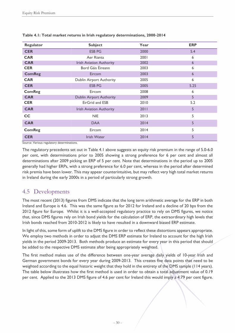
Equity Risk Premium
- 30 -
Table 4.1: Total market returns in Irish regulatory determinations, 2000-2014
Regulator Subject Year ERP
CER ESB PG 2000 5.4
CAR Aer Rianta 2001 6
CAR Irish Aviation Authority 2002 6
CER Bord Gáis Éireann 2003 6
ComReg Eircom 2003 6
CAR Dublin Airport Authority 2005 6
CER ESB PG 2005 5.25
ComReg Eircom 2008 6
CAR Dublin Airport Authority 2009 5
CER EirGrid and ESB 2010 5.2
CAR Irish Aviation Authority 2011 5
CC NIE 2013 5
CAR DAA 2014 5
ComReg Eircom 2014 5
CER Irish Water 2014 5
Source: Various regulatory determinations.
The regulatory precedents set out in Table 4.1 above suggests an equity risk premium in the range of 5.0-6.0
per cent, with determinations prior to 2005 showing a strong preference for 6 per cent and almost all
determinations after 2009 picking an ERP of 5 per cent. Note that determinations in the period up to 2005
generally had higher ERPs, with a strong preference for 6.0 per cent, whereas in the period after determined
risk premia have been lower. This may appear counterintuitive, but may reflect very high total market returns
in Ireland during the early 2000s in a period of particularly strong growth.
4.5 Developments
The most recent (2013) figures from DMS indicate that the long term arithmetic average for the ERP in both
Ireland and Europe is 4.6. This was the same figure as for 2012 for Ireland and a decline of 20 bps from the
2012 figure for Europe. Whilst it is a well-accepted regulatory practice to rely on DMS figures, we notice
that, since DMS figures rely on Irish bond yields for the calculation of ERP, the extraordinary high levels that
Irish bonds reached from 2010-2012 is likely to have resulted in a downward biased ERP estimate.
In light of this, some form of uplift to the DMS figure in order to reflect these distortions appears appropriate.
We employ two methods in order to adjust the DMS ERP estimate for Ireland to account for the high Irish
yields in the period 2009-2013. Both methods produce an estimate for every year in this period that should
be added to the respective DMS estimate after being appropriately weighted.
The first method makes use of the difference between one-year average daily yields of 10-year Irish and
German government bonds for every year during 2009-2013. This creates five data points that need to be
weighted according to the equal historic weight that they hold in the entirety of the DMS sample (114 years).
The table below illustrates how the first method is used in order to obtain a total adjustment value of 0.19
per cent. Applied to the 2013 DMS figure of 4.6 per cent for Ireland this would imply a 4.79 per cent figure.
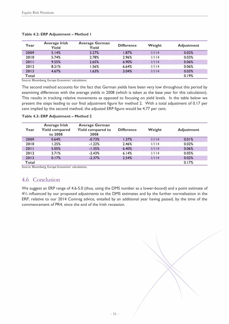
Equity Risk Premium
- 31 -
Table 4.2: ERP Adjustment – Method 1
Year Average Irish
Yield
Average German
Yield Difference Weight Adjustment
2009 5.14% 3.27% 1.87% 1/114 0.02%
2010 5.74% 2.78% 2.96% 1/114 0.03%
2011 9.55% 2.65% 6.90% 1/114 0.06%
2012 8.21% 1.56% 6.64% 1/114 0.06%
2013 4.67% 1.63% 3.04% 1/114 0.03%
Total 0.19% Source: Bloomberg, Europe Economics’ calculations.
The second method accounts for the fact that German yields have been very low throughout this period by
examining differences with the average yields in 2008 (which is taken as the base year for this calculation).
This results in tracking relative movements as opposed to focusing on yield levels. In the table below we
present the steps leading to our final adjustment figure for method 2. With a total adjustment of 0.17 per
cent implied by the second method, the adjusted ERP figure would be 4.77 per cent.
Table 4.3: ERP Adjustment – Method 2
Year
Average Irish
Yield compared
to 2008
Average German
Yield compared to
2008
Difference Weight Adjustment
2009 0.64% -0.73% 1.37% 1/114 0.01%
2010 1.25% -1.22% 2.46% 1/114 0.02%
2011 5.05% -1.35% 6.40% 1/114 0.06%
2012 3.71% -2.43% 6.14% 1/114 0.05%
2013 0.17% -2.37% 2.54% 1/114 0.02%
Total 0.17% Source: Bloomberg, Europe Economics’ calculations.
4.6 Conclusion
We suggest an ERP range of 4.6-5.0 (thus, using the DMS number as a lower-bound) and a point estimate of
4¾ influenced by our proposed adjustments to the DMS estimates and by the further normalisation in the
ERP, relative to our 2014 Comreg advice, entailed by an additional year having passed, by the time of the
commencement of PR4, since the end of the Irish recession.

Equity Beta and Cost of Equity
- 32 -
5 Equity Beta and Cost of Equity
5.1 PR3, Mid-Term Review and Stakeholder Submissions regarding asset beta
At PR3 we recommended an asset beta of 0.3, the same figure being used at the Mid-Term Review.
For PR4 the stakeholder submissions were: ESBN proposed an asset beta of 0.36 whilst EirGrid
proposed an asset beta of 0.4.
5.2 Analysis of risks faced by the TAO, DSO and TSO
The applicability of a RAB-WACC approach or a margin alternative is considered in a separate document.
This section explores the issues arising from the following question: if a RAB-WACC approach is
methodologically appropriate and there is a correctly specified RAB, what is the right WACC?
5.2.1 The transmission and distribution networks
Transmission asset owner (TAO) – ESB networks
ESB Networks24 is the licensed owner of the transmission system - the transmission asset owner (TAO).
The role of the TAO is to ensure that the transmission system is developed and maintained in accordance
with the requirements set down by the transmission system operator (EirGrid).
The TAO has responsibility for the management of the transmission capital and maintenance work
programmes. This includes the building of new high-voltage substations and their associated overhead lines
and underground cables. It also involves responding to network faults and carrying out planned maintenance
and refurbishment works on these assets.
The TSO EirGrid is responsible for operating the network of high-voltage transmission lines and substations
to transport power from the various electricity generators to where it is needed and for setting out the
planned development needs of the transmission network.
There is a legal agreement in place between EirGrid and ESB Networks (the "Infrastructure Agreement")
which sets out the terms under which ESB Networks provides infrastructure services to EirGrid. The
agreement was approved by CER and came into effect on 1 July 2006 – the same date as the legal
establishment of EirGrid as the TSO.
Transmission system operator (TSO) – EirGrid
EirGrid is the independent state-owned body licensed by the CER to act as transmission system operator
(TSO).
The electricity transmission system (commonly known as the national grid) is a high voltage network for the
transmission of bulk electricity supplies around Ireland. Generally the high voltage lines deliver electricity
from Ireland's generation sources to the transformer stations, where the electricity voltage is reduced and
taken through the distribution system to individual customers' premises.
24 ESB Networks is a ring fenced subsidiary within ESB Group.

Equity Beta and Cost of Equity
- 33 -
EirGrid is responsible for the operation, development and maintenance of the system. The TSO also offers
terms and levies charges for connection to and use of the transmission system. These are regulated by the
CER.
The Connection Agreement is structured in three parts: the Connection Agreement contains the specific
provisions in respect of connecting both generation and demand customers; the General Conditions contains
the general provisions of the Connection Agreement; and Schedule 10 contains construction and
commissioning provisions.
Distribution system operator (DSO) – ESB Networks Ltd
ESB Networks Ltd is the licensed operator of the electricity distribution system – the distribution system
operator (DSO).
The distribution network is the medium- and low-voltage electricity network used to deliver electricity to
connection points such as houses, workplaces and street lights.
ESB Networks as Distribution Asset Owner (DAO) owns and is responsible for building, maintaining and
operating the entire distribution level network infrastructure. This includes all overhead electricity lines,
poles and underground cables used to bring power to Ireland's customers.
Distribution tariffs are the charges paid for using the distribution system. The tariffs are paid by the suppliers
who use the system (and are ultimately passed on to customers). The CER sets the tariffs to be applied for
use of the network. Distribution tariffs are reviewed annually. The CER periodically carries out full reviews
of the costs that ESB Networks incurs owning, maintaining and operating the distribution system to ensure
that only equitable levels of costs are collected through the distribution tariffs (the price control review).
5.2.2 Underlying business risks
We now discuss the underlying risks in carrying out the business activities of the TAO, TSO and DSO. As
only systematic risks affect the appropriate cost of capital, we focus on this type of risk. However, we first
include a brief outline of some of the specific risks which may affect the networks.
Specific risks — those risks that only apply to a particular asset class and which are not correlated with
the overall returns of the market portfolio. As these risks can be diversified by investors they do not
affect a company’s cost of capital
Systematic risk — also known as market or non-diversifiable risk, is risk that is characteristic of an entire
market. As it cannot be diversified away by investors, the extent of the systematic risk affects a company’s
cost of capital.25 Examples of risks with a systematic element affecting the transmission and distribution
networks are discussed below.
Systematic risk can be divided into cost risk and demand risk. Of these, in most industries the dominant
form of systematic risk is demand risk.
Demand volatility
There are a number of factors that can affect the demand for the services of the TAO, TSO and DSO. Types
of demand risk affecting the transmission and distribution networks are:
the number of customers (both existing and new connections);
the voltage transported; and
the length of network required.
25 As explained in section 1, exposure to systematic risk is captured in the CAPM equation by the size of company’s
equity beta, which is multiplied by the market risk premium and added to the risk-free rate to determine the cost
of equity.

Equity Beta and Cost of Equity
- 34 -
Although there would be specific factors affecting demand such as environmental legislation, there would also
be systematic components to demand – for example, a country’s GDP which could affect the demand for
energy. Growth in the Republic of Ireland’s GDP is also likely to be correlated with the number of new
premises built and hence the number of new connections.
The demand for EirGrid’s services is derived from demand for electricity in Ireland and thus demand from
ESB and generation and load directly connected to the transmission system. But not all fluctuations in
electricity demand, either voltage transported or number of customers, will induce fluctuations in demand
for EirGrid’s services, because the management of the transmissions assets will be fairly consistent even as
output varies. It is therefore natural to assume that EirGrid’s systematic demand risk exposure will tend to
be less than that of ESB.
Bad debts
Customer defaults affect a company’s profitability. The proportion of customers defaulting on their utility
bills is likely to rise in a recession and hence bad debts can be a systematic risk for the industry, primarily
affecting the suppliers of electricity
Customers are also more likely to fall behind on their bills in a recession, even if their bills are still ultimately
paid. This will be costly for companies as cash will be received later rather than sooner, either requiring
companies to raise working capital to cover their cash requirements (with associated financing costs), or
meaning that companies forego the opportunity to earn returns on this cash during the period of delay.
Changes in input costs
Changes in input costs affect the revenues of the TAO, TSO and DSO. Input costs include the costs of
construction materials as well as the costs of paying wages to staff. The networks may also be affected by
changes in oil prices and related factor inputs.
Changes in inputs such as wages are systematic in nature to the extent that they affect the whole economy.
However, there may be a specific element to certain inputs if only particular categories of that input are
affected (for example, the wages of construction workers).
Interest rate movements
Changes in interest rates affect the whole economy and are hence a systematic risk.
Interest rates can affect the costs of raising finance, and the repayment terms of existing debt where debt has
a floating rather than a fixed interest rate. Bond prices move inversely to interest rates, with bond prices
being lower when interest rates are high and vice versa. This is because with a static coupon bond prices
and bond yields are inversely related (the higher the price of the bond, the lower the real yield); and bond
holders are prepared to accept a lower rate of return (yield) when interest rates are low; but demand a
higher yield when interest rates are high.
Interest rates will have direct effects on a company’s systematic risk but also indirect effects as they may have
an impact on demand volatility and input costs.
Changes in inflation/ deflation
Changes in inflation affect the whole economy and therefore represent a systematic risk. The inflation rate
affects the real amount which a firm ends up repaying on nominal debt. Inflation may also affect input costs.
As a result of the recent financial crisis, the European Central Bank is close to announcing its quantitative
easing program in order to combat deflationary pressures. Deflation increases the real amount repayable on
nominal debt, although companies may benefit from lower input costs.
Like interest rates, the rate of inflation will also have direct effects on a company’s systematic risk but also
indirect effects on other factors such as demand volatility. Inflation also affects revenues through indexation.

Equity Beta and Cost of Equity
- 35 -
The extent to which a company is affected by interest rate movements and changes in inflation will be
influenced by the amount of finance it needs to raise. Companies which have to undertake large amounts of
investment may therefore face higher risks.
5.2.3 Other Factors affecting risk exposure
There are certain factors that affect a company’s exposure to systematic risk. These include the regulatory
framework and cost structure.
Regulatory framework
A regulatory framework can either increase or decrease a company’s exposure to systematic risk when
compared with an unregulated company performing similar functions.
A firm allowed full cost pass-through or with rate-of-return regulation faces no increase in systematic risk if
there is cost uncertainty.
Whether the price control takes the form of a price cap or a revenue cap affects a company’s systematic risk.
The two alternatives work as follows:
Price cap – the regulator agrees a fixed set of tariffs. The revenue which the company earns from these
tariffs would depend on market volumes. Under a pure price cap approach, the company is fully exposed
to the revenue consequences of any change in market volumes. In other words, its revenue would
increase if market volumes increased, but would fall if market volumes decreased.
However, price cap regulation decreases a firm’s beta when compared with an unregulated firm. This is
because profits rise less for the regulated firm compared with the unregulated firm when there are
positive shocks to demand due to the price cap placing a limit on price rises, but profits will fall due to
negative shocks in the same way as for an unregulated firm since prices can (at least in theory) fall below
the cap. Overall, profits for the regulated firm are less variable (and on average lower, due to not being
able to take full advantage of upside shocks) than when the firm is unregulated. This lower variability in
profits leads to a lower beta for the regulated firm when compared to an unregulated firm.
Revenue cap – the regulator would agree the revenues that the company should be allowed to earn.
Tariffs would be calculated so as to recover these revenues on the basis of projected market volumes.
However, in the event that out-turn market volumes differed from these projections, any over- or under-
recovery of revenue would be taken into account in finalising the tariffs for the following year. As tariffs
are changed annually (to allow a set level of revenues to be earned) the company is exposed to less
systematic risk than companies with a pure price cap.
Regulators are not necessarily restricted to choosing between the pure price cap and revenue cap approaches
described above, since it is also possible to employ a hybrid approach. For instance, a price control could be
set such that 50 per cent of allowed revenue is fixed, with the company exposed to changes in market
volumes in relation to the other 50 per cent. This type of arrangement is sometimes referred to as including
a “volume driver” within the price control.
There are a number of mechanisms that a regulator can use to reduce a company’s exposure to systematic
risk. These include the type of price cap, cost pass through items and revenue drivers.
Cost structure
Another risk consideration is related to the concept of operation leverage. A firm’s operating leverage refers
to the level of its fixed costs relative to variable costs. To see how this relates to beta, first note that the
present value of an asset is equal to the present value of revenues, less the present values of fixed and variable
costs:
NPV(asset) = NPV(revenue) – NPV(fixed costs) – NPV(variable costs)

Equity Beta and Cost of Equity
- 36 -
This can also be expressed with respect to the present value of revenue:
NPV(revenue) = NPV(asset) + NPV(fixed costs) + NPV(variable costs)
Given this expression, the beta of the present value of the asset’s revenue (as distinct from the beta of the
present value of the asset itself) can then be expressed as
βREV = [NPV(asset) / NPV(revenue)]· βASSET + [NPV(fixed costs) / NPV(revenue)]· βFIXED
+ [NPV(variable costs) / NPV(revenue)]· βVARIABLE
By definition, the beta of fixed costs should be approximately zero, while the betas of revenue and variable
costs should be approximately equal as they both change in response to output. Noting these, and rearranging
the above expression implies
βASSET = βREV· (1 + [NPV(fixed costs) / NPV(asset)])
This states, therefore, that firms with a high ratio of fixed costs to asset value have higher asset betas.
Even though it would possible in principle to assess whether a difference in operating leverage between
EirGrid and ESBN leads to wedge between the asset betas of the two companies, we are unable to conduct
such analysis because we lack (as illustrated in in details in a separate note) an estimate of EirGrid’s asset
value that would be relevant and appropriate for the purpose.
5.2.4 Conclusion
We have identified no compelling reason to believe that there is a material difference between the systematic
risk exposures of the TAO, TSO and DSO. Theoretical considerations might suggest that the TSO should
be expected to be subject to less demand risk that the other players. On the other hand, the impact of
differences in operating leverage, which could be material, are unknown and unknowable.
Our judgment is that, if the enterprise value is specified correctly, the rate of return on total assets (as
measured by enterprise value) is likely to be similar between the TAO, TSO, and DSO. However, we note
that in an accompanying document we explain our view that it can be argued that EirGrid’s enterprise value
may not be fully reflected in its RAB.
5.3 Methodology
We discuss here, general methodological issue for the estimation of asset beta. More specifically, this
subsection is organised as follows:
Use of comparator analysis.
Empirical specification.
Choice of the appropriate market portfolio.
Estimation period.
Equity beta adjustments.
De-levering of equity beta into asset beta.
Gearing measures used for un-lever equity beta.
Re-levering asset beta into equity beta.
5.3.1 Use of comparator analysis
For publicly listed regulated entities it is common practice to estimate asset beta from direct market data.
Since ESBN and EirGrid are not listed, their asset betas must necessarily be inferred from a set of relevant
comparators – ideally, listed companies carrying out comparable activities and subject to similar economic

Equity Beta and Cost of Equity
- 37 -
regulation. Consistently with the approach used in PR3 and the mid-term WACC review, the set of relevant
comparators is composed of utilities that operate in the European energy sector and own electricity or gas
transmission and distribution networks. In addition, we have included comparator companies that operate
in the UK water sector, reflecting the similarities between water and energy networks.26 The network
businesses of these comparators would in many cases be subject to broadly similar RPI-X regulation. Based
on these similarities, we consider that these comparators are likely to be exposed to a similar level of
systematic risk.
A caveat surrounding this sample of comparators is that many of the companies also operate in other parts
of the value chain (i.e. generation and supply) as well as owning and operating transmission and distribution
networks. Some companies may also be involved in non-energy activities. The table below lists the
comparators used in this report and indicates whether they were used in 2010 and/or the mid-term Review.
Table 5.1: List of comparators
Company Sector Country
National Grid Electricity UK
Severn Trent Water UK
SSE Gas and Electricity UK
Pennon** Water UK
Centrica** Gas and Electricity UK
United Utilities** Water UK
Scottish Power* Gas and Electricity UK
Viridian* Gas and Electricity UK
ENEL Energy IT
A2A** Electricity IT
Hera** Gas and Electricity IT
Terna** Electricity IT
Snam rete gas* Gas and Electricity IT
Endesa** Energy ES
Gas Natural** Gas and Electricity ES
Red Electrica Electricity ES
REN* Gas and Electricity PT
EDP** Energy PT
Veolia** Water FR
EDF Energy FR
GDF Suez Gas and Electricity FR
RWE Energy DE
EnBW** Gas and Electricity DE
E.ON Gas and Electricity DE
Note: * refers to companies that were only included in the 2010 report, ** refers to companies that were only included in the mid-term review.
Companies with no asterisks were included in both reports.
Beta estimates for comparators can either be taken direct from existing sources (e.g. Bloomberg or the LBS
Risk Management Service), or they can be estimated from data on company and stock market returns. The
advantage of the former is that it is less resource-intensive, whereas the advantage of the latter is that it gives
greater control over how the estimation is carried out. We have opted for the latter approach, which is
consistent with the methodology employed for the Mid-Term review.
26 The three UK water and sewerage companies are Severn Trent, Pennon and United Utilities. These companies are
included as comparators due to the similarities in activities of energy and water companies in terms of network
activities, exposure to volume risk and the need for infrastructure investment.

Equity Beta and Cost of Equity
- 38 -
5.3.2 Empirical specification
The (raw) equity beta (𝛽𝑖) measures the covariance between the company (i) return over the safe rate with
the market return over the safe rate. The equation to be estimated is usually:
𝑅𝑖,𝑡 = 𝛼 + 𝛽𝑖𝑅𝑚,𝑡 + 𝜀𝑖𝑡
where 𝑅𝑖,𝑡 is the log excess return on asset i at date t (log return net of the logarithmic safe rate), 𝑅𝑚,𝑡 is the
log excess return on the market, 𝛼 is a constant, 𝛽𝑖 is the equity beta, and 𝜀𝑖𝑡 is an error term — the non-
systematic component of the return to the asset — which may display both heteroskedasticity and
autocorrelation.
The excess return 𝑅𝑖,𝑡 is constructed as a data manipulation prior to estimation and is defined as:
𝑅𝑖,𝑡 = 𝑙𝑛 (𝑃𝑡 + 𝐷𝑡
𝑃𝑡−1) − ln (1 + 𝑅𝑓,𝑡)
where 𝑃𝑡 is the price today, 𝐷𝑡 is dividend per share that becomes known today, 𝑃𝑡−1 is the price yesterday,
and 𝑅𝑓,𝑡 is the safe rate available today.
Since a substantial body of academic and regulatory literature supports that the idea the potential bias from
not netting off the risk free rate is negligible in most cases, we have therefore opted for carrying out the
estimations without netting off the risk-free rate from individual share and market index returns.
5.3.3 Choice of the market portfolio
With regard to the market portfolio for calculating 𝑅𝑚,𝑡, we have chosen the following domestic equity
markets indices:
Deutsche Börse AG German Stock Index (Germany).
CAC 40 Index (France).
FSTE MIB Index (Italy).
PSI All-Share Index (Portugal).
IBEX 35 Index (Spain).
FTSE All-Share Index (UK).
As a cross-check betas were estimated also on a European wide market index (i.e. the MSCI-All Countries-
Europe Index).
5.3.4 Data frequency
In principle daily data are preferred to weekly, monthly, or yearly data because they allow estimates on larger
samples. However, as Smithers & Co (2003) illustrate, a concern with the use of daily data is represented
by the possibility of returns being serially correlated, while this risk is likely to be less material in the presence
of weekly or monthly data. Nevertheless, Smithers & Co (2003) point out that it is possible to control for
autocorrelation by using the Newey-West correction method in order to obtain consisted standard errors.
Furthermore, if there are reasons to believe that heteroskedasticity may also be a problem, White’s
heteroskedasticity corrected error terms can also be computed.
We have therefore decided to estimate equity betas on daily data, and we have carried out the estimations
controlling for both heteroskedasticity and serial correlation.

Equity Beta and Cost of Equity
- 39 -
5.3.5 Estimation period
Equity betas vary over time. This might be because of changes in gearing or changes in the underlying
correlations between company and aggregate returns (i.e. asset betas). It would be sensible, therefore, to
choose an estimation window that is as recent as possible, because today’s observation is the forward looking
estimate, while still giving reasonably accurate estimates.27
Smithers & Co (2003) investigate the matter, noting that gains in estimation accuracy become less as more
observations are added. For example, going from one year to two years of daily data (i.e. 250 observations
to 500 observations) will reduce the standard error by 40 per cent, but going from three to four years only
reduces the error by 15 per cent.
It would be possible to use an explicit time-series estimation technique to account for the time variation.
However, these techniques, as noted by Smithers & Co (2003), are susceptible to over-fitting and can find
apparent time variation where none exists. The techniques are also non-linear and not widely used for
regulatory purposes.
We have therefore adopted the Smithers & Co (2003) recommendation and have based our analysis primarily
on two years rolling betas. As an additional cross-check we also estimated betas on 1-year and 5-year
windows of daily data.
5.3.6 Adjustments to estimated betas
Two main adjustments, the so-called Bayesian and Blume adjustments, have been used in some past
estimations of beta, with the effect of bringing the estimated betas closer to one.
The argument for Bayesian adjustment is that the estimation of beta ignores the fact that the beta of an
average company is by definition equal to one. The Bayesian adjustment takes account of measurement
uncertainty (as estimated explicitly in the calculation of the raw beta) by employing a weighted average
between the beta estimate for the company and a constructed average beta for the market as a whole that
would be equal to one. The weights are based on the relative uncertainty in measurement — the higher the
uncertainty in the company beta estimates relative to the variance of all betas in the market, the less weight
is placed on the company beta. The Blume adjustment is based on an empirical observation (made in 1971)
that betas tended to move towards one over a (long) time period. Mean reversion is sometimes offered as
an explanation for this observed movement. In later investigations, however, Blume found that the reasons
for the movement in the betas had to be explained by some real changes in the perceived risks of the
companies — the tendency for companies to evolve could mean that companies of extreme risk (high or
low) tend to have less extreme risks over time.
Our view is that the use of the Blume adjustment is arbitrary and inappropriate. While a Bayesian adjustment
has a stronger theoretical rationale, Smithers & Co (2003) found that in practice it may not make much
difference if daily data are used in the estimation.
5.3.7 De-levering equity beta into asset beta
When comparing the betas of different firms, one has to take into account the different gearing levels that
firms choose since — all other things being equal — a firm with higher gearing will exhibit a higher equity
beta. Therefore, unless one controls for this effect, there is a danger of confusing the risk that comes from
high leverage with the underlying systematic risk that a firm faces by virtue of the nature of its activities.
27 We note that the single point estimate for beta will embody expectations for returns over the lifetime of the assets
involved. There is thus no intrinsic tension between the use of a beta point estimate and its application to a five-year
price control.
Equity Beta and Cost of Equity
- 40 -
Asset betas are calculated in order to control for the effect of differing levels of gearing. An asset beta is a
hypothetical measure of the beta that a firm would have if it were financed entirely by equity. By comparing
different firms’ asset betas it is possible to isolate shareholders’ perceptions of underlying systematic risk,
and carry out an assessment of the relative riskiness of different companies after controlling for gearing.
De-levered asset betas are calculated using the following formula:
𝛽𝐴,𝑖 = (1 − 𝑔𝑖)𝛽𝑖 + 𝑔𝑖𝛽𝑖𝐷
where 𝛽𝐴,𝑖 is a firm’s asset beta, 𝛽𝑖 is a firm’s raw equity beta, 𝑔𝑖 is the company’s gearing, and 𝛽𝑖𝐷
is the firm’s
debt beta.28 De-levered asset betas for comparators have been calculated assuming zero debt betas.
5.3.8 Gearing measures used for de-levered asset beta
An important practical issue relates to the choice of gearing measure which is used to de-lever the equity
betas in order to estimate asset betas. In particular, a choice has to be made about the measure of asset
value which is going to be used in the denominator of the gearing measure.
At a conceptual level, our preferred measure of gearing would be net debt to RAB, given that the TAO, TSO
and DSO are subject to RAB-based price regulation. However, many of the comparator companies include
generation and supply businesses as well as network businesses, and in many cases there will not be a RAB
figure available for businesses operating in these parts of the supply chain (e.g. generation and supply are not
subject to RAB-based price regulation in the UK). Further, where the comparator company owns a number
of network businesses, there may be no readily available RAB figure at a group level even if a RAB exists for
some or all of the subsidiary companies.
We have considered two of the gearing measures available in Bloomberg:
total debt / total assets, where asset values appear to be based on book values in statutory company
accounts; and
total debt / total capital, where total capital appears to be based on net debt and market capitalisation.
In our view, the asset values in statutory company accounts do not form a good basis for measuring gearing.
They may differ substantially from asset values that would be included in a RAB for a number of reasons –
for instance, unlike the RAB, asset values in statutory accounts are not indexed to inflation.
By contrast, under certain conditions (e.g. including that the regulatory WACC reflects the company’s true
market cost of capital, and that there is no under-performance or out-performance against regulatory
assumptions on opex and capex), one would expect the market value of a company to be in line with its RAB.
While these conditions will not always hold in practice, we nonetheless consider that using a gearing measure
based on the market value of a company will tend to reflect more closely our ideal measure of gearing (net
debt / RAB) than one based on the book value of assets in statutory accounts.
In the light of this, we have used Bloomberg data on total debt / total capital as expressed through net
debt/(net debt + market capitalisation) as our measure of gearing for most companies.
5.3.9 Re-levering asset beta into equity beta
Once, based on comparators analysis, a decision is taken on what are the appropriate asset beta values for
ESBN and EirGrid, these can be expressed back as equity beta through a re-levering exercise which makes
28 The debt beta measures the covariance between the return on a company’s debt with the market return. In this
work we assume a debt beta of zero (this is in keeping with a number of regulatory precedents), and also carry out
sensitivity analysis assuming non-zero debt betas based on companies’ credit ratings.
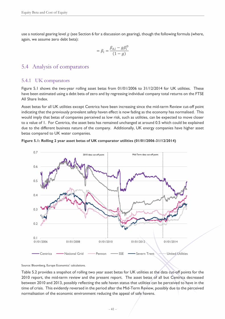
Equity Beta and Cost of Equity
- 41 -
use a notional gearing level 𝑔 (see Section 6 for a discussion on gearing), though the following formula (where,
again, we assume zero debt beta):
= 𝛽𝑖 =𝛽𝐴,𝑖 − 𝑔𝛽𝑖
𝐷
(1 − 𝑔)
5.4 Analysis of comparators
5.4.1 UK comparators
Figure 5.1 shows the two-year rolling asset betas from 01/01/2006 to 31/12/2014 for UK utilities. These
have been estimated using a debt beta of zero and by regressing individual company total returns on the FTSE
All Share Index.
Asset betas for all UK utilities except Centrica have been increasing since the mid-term Review cut-off point
indicating that the previously prevalent safety haven effect is now fading as the economy has normalised. This
would imply that betas of companies perceived as low risk, such as utilities, can be expected to move closer
to a value of 1. For Centrica, the asset beta has remained unchanged at around 0.5 which could be explained
due to the different business nature of the company. Additionally, UK energy companies have higher asset
betas compared to UK water companies.
Figure 5.1: Rolling 2 year asset betas of UK comparator utilities (01/01/2006-31/12/2014)
Source: Bloomberg, Europe Economics’ calculations.
Table 5.2 provides a snapshot of rolling two year asset betas for UK utilities at the data cut-off points for the
2010 report, the mid-term review and the present report. The asset betas of all but Centrica decreased
between 2010 and 2013, possibly reflecting the safe haven status that utilities can be perceived to have in the
time of crisis. This evidently reversed in the period after the Mid-Term Review, possibly due to the perceived
normalisation of the economic environment reducing the appeal of safe havens.
0.1
0.2
0.3
0.4
0.5
0.6
0.7
01/01/2006 01/01/2008 01/01/2010 01/01/2012 01/01/2014
Centrica National Grid Pennon SSE Severn Trent United Utilities
Mid-Term data cut-off point2010 data cut-off point
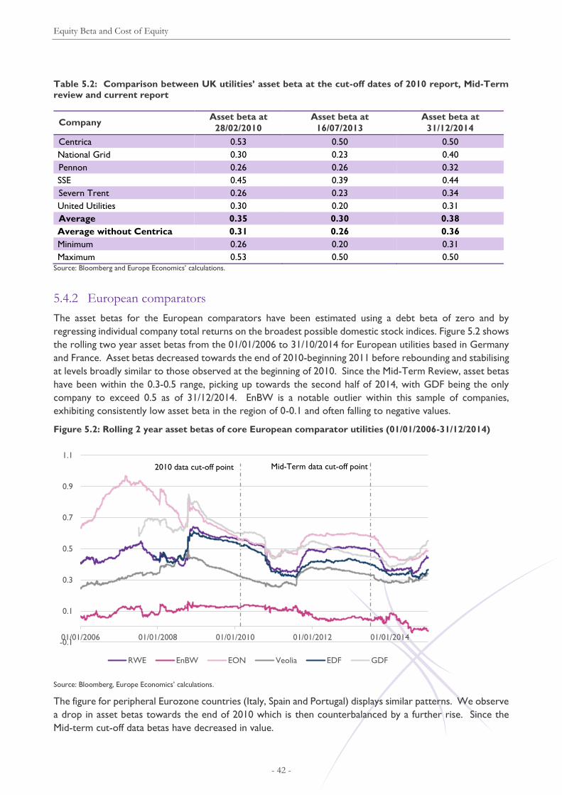
Equity Beta and Cost of Equity
- 42 -
Table 5.2: Comparison between UK utilities’ asset beta at the cut-off dates of 2010 report, Mid-Term
review and current report
Company Asset beta at
28/02/2010
Asset beta at
16/07/2013
Asset beta at
31/12/2014
Centrica 0.53 0.50 0.50
National Grid 0.30 0.23 0.40
Pennon 0.26 0.26 0.32
SSE 0.45 0.39 0.44
Severn Trent 0.26 0.23 0.34
United Utilities 0.30 0.20 0.31
Average 0.35 0.30 0.38
Average without Centrica 0.31 0.26 0.36
Minimum 0.26 0.20 0.31
Maximum 0.53 0.50 0.50 Source: Bloomberg and Europe Economics’ calculations.
5.4.2 European comparators
The asset betas for the European comparators have been estimated using a debt beta of zero and by
regressing individual company total returns on the broadest possible domestic stock indices. Figure 5.2 shows
the rolling two year asset betas from the 01/01/2006 to 31/10/2014 for European utilities based in Germany
and France. Asset betas decreased towards the end of 2010-beginning 2011 before rebounding and stabilising
at levels broadly similar to those observed at the beginning of 2010. Since the Mid-Term Review, asset betas
have been within the 0.3-0.5 range, picking up towards the second half of 2014, with GDF being the only
company to exceed 0.5 as of 31/12/2014. EnBW is a notable outlier within this sample of companies,
exhibiting consistently low asset beta in the region of 0-0.1 and often falling to negative values.
Figure 5.2: Rolling 2 year asset betas of core European comparator utilities (01/01/2006-31/12/2014)
Source: Bloomberg, Europe Economics’ calculations.
The figure for peripheral Eurozone countries (Italy, Spain and Portugal) displays similar patterns. We observe
a drop in asset betas towards the end of 2010 which is then counterbalanced by a further rise. Since the
Mid-term cut-off data betas have decreased in value.
-0.1
0.1
0.3
0.5
0.7
0.9
1.1
01/01/2006 01/01/2008 01/01/2010 01/01/2012 01/01/2014
RWE EnBW EON Veolia EDF GDF
2010 data cut-off point Mid-Term data cut-off point
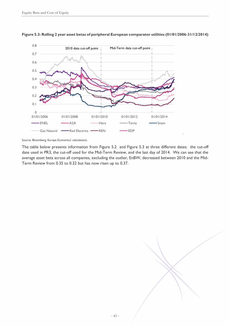
Equity Beta and Cost of Equity
- 43 -
Figure 5.3: Rolling 2 year asset betas of peripheral European comparator utilities (01/01/2006-31/12/2014)
.
Source: Bloomberg, Europe Economics’ calculations.
The table below presents information from Figure 5.2 and Figure 5.3 at three different dates; the cut-off
date used in PR3, the cut-off used for the Mid-Term Review, and the last day of 2014. We can see that the
average asset beta across all companies, excluding the outlier, EnBW, decreased between 2010 and the Mid-
Term Review from 0.35 to 0.32 but has now risen up to 0.37.
0
0.1
0.2
0.3
0.4
0.5
0.6
0.7
0.8
01/01/2006 01/01/2008 01/01/2010 01/01/2012 01/01/2014
ENEL A2A Hera Terna Snam
Gas Natural Red Electrica REN EDP
2010 data cut-off point Mid-Term data cut-off point
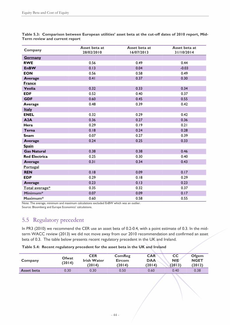
Equity Beta and Cost of Equity
- 44 -
Table 5.3: Comparison between European utilities’ asset beta at the cut-off dates of 2010 report, Mid-
Term review and current report
Company Asset beta at
28/02/2010
Asset beta at
16/07/2013
Asset beta at
31/10/2014
Germany
RWE 0.56 0.49 0.44
EnBW 0.13 0.04 -0.03
EON 0.56 0.58 0.49
Average 0.41 0.37 0.30
France
Veolia 0.32 0.33 0.34
EDF 0.52 0.40 0.37
GDF 0.60 0.45 0.55
Average 0.48 0.39 0.42
Italy
ENEL 0.32 0.29 0.42
A2A 0.36 0.27 0.36
Hera 0.29 0.19 0.21
Terna 0.18 0.24 0.28
Snam 0.07 0.27 0.39
Average 0.24 0.25 0.33
Spain
Gas Natural 0.38 0.38 0.46
Red Electrica 0.25 0.30 0.40
Average 0.31 0.34 0.43
Portugal
REN 0.18 0.09 0.17
EDP 0.29 0.18 0.29
Average 0.23 0.13 0.23
Total average* 0.35 0.32 0.37
Minimum* 0.07 0.09 0.17
Maximum* 0.60 0.58 0.55
Note: The average, minimum and maximum calculations excluded EnBW which was an outlier.
Source: Bloomberg and Europe Economics’ calculations.
5.5 Regulatory precedent
In PR3 (2010) we recommend the CER use an asset beta of 0.2-0.4, with a point estimate of 0.3. In the mid-
term WACC review (2013) we did not move away from our 2010 recommendation and confirmed an asset
beta of 0.3. The table below presents recent regulatory precedent in the UK and Ireland.
Table 5.4: Recent regulatory precedent for the asset beta in the UK and Ireland
Company Ofwat
(2014)
CER
Irish Water
(2014)
ComReg
Eircom
(2014)
CAR
DAA
(2014)
CC
NIE
(2013)
Ofgem
NGET
(2012)
Asset beta 0.30 0.30 0.50 0.60 0.40 0.38
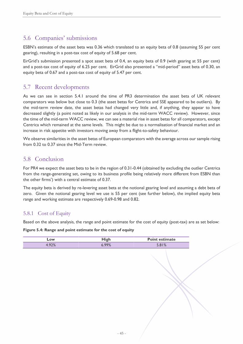
Equity Beta and Cost of Equity
- 45 -
5.6 Companies’ submissions
ESBN’s estimate of the asset beta was 0.36 which translated to an equity beta of 0.8 (assuming 55 per cent
gearing), resulting in a post-tax cost of equity of 5.68 per cent.
EirGrid’s submission presented a spot asset beta of 0.4, an equity beta of 0.9 (with gearing at 55 per cent)
and a post-tax cost of equity of 6.25 per cent. EirGrid also presented a “mid-period” asset beta of 0.30, an
equity beta of 0.67 and a post-tax cost of equity of 5.47 per cent.
5.7 Recent developments
As we can see in section 5.4.1 around the time of PR3 determination the asset beta of UK relevant
comparators was below but close to 0.3 (the asset betas for Centrica and SSE appeared to be outliers). By
the mid-term review date, the asset betas had changed very little and, if anything, they appear to have
decreased slightly (a point noted as likely in our analysis in the mid-term WACC review). However, since
the time of the mid-term WACC review, we can see a material rise in asset betas for all comparators, except
Centrica which remained at the same levels. This might be due to a normalisation of financial market and an
increase in risk appetite with investors moving away from a flight-to-safety behaviour.
We observe similarities in the asset betas of European comparators with the average across our sample rising
from 0.32 to 0.37 since the Mid-Term review.
5.8 Conclusion
For PR4 we expect the asset beta to be in the region of 0.31-0.44 (obtained by excluding the outlier Centrica
from the range-generating set, owing to its business profile being relatively more different from ESBN than
the other firms’) with a central estimate of 0.37.
The equity beta is derived by re-levering asset beta at the notional gearing level and assuming a debt beta of
zero. Given the notional gearing level we use is 55 per cent (see further below), the implied equity beta
range and working estimate are respectively 0.69-0.98 and 0.82.
5.8.1 Cost of Equity
Based on the above analysis, the range and point estimate for the cost of equity (post-tax) are as set below:
Figure 5.4: Range and point estimate for the cost of equity
Low High Point estimate
4.92% 6.99% 5.81%

Capital Structure
- 46 -
6 Capital Structure
6.1 PR3, Mid-Term Review and Stakeholder Submissions
At PR3 and the mid-term review the gearing was 0.55. At PR4 both ESBN and EirGrid propose a
gearing of 0.55.
6.2 Introduction
In calculating a WACC estimate, it is necessary to make an assumption about the gearing level of the company
so as to know the weight which should be placed respectively on the cost of equity and the cost of debt.
However, as discussed below, the choice of gearing does not necessarily affect the vanilla WACC since both
the cost of equity and the cost of debt change with gearing. The choice of gearing does, however, affect the
tax liabilities which the CER has to allow for within price limits.
The notional level of gearing on which the WACC calculation is based is not intended to represent second-
guessing of companies’ decisions about their optimal financing structure, or to provide any guidance on the
gearing level that firms should adopt.
6.3 Capital structure and CAPM
The starting point in thinking about the effect of gearing is the Modigliani-Miller insight (MMI) that the riskiness
of a company depends on the riskiness of its real cash-flows — volatility in the costs and in the demand for
its products. The implication is that where there are no taxes, incentive or information problems, the way a
project or firm is financed does not affect its value or its cost of capital — the market value of any firm is
independent of its capital structure. This is because the overall risk on the company’s asset base, the asset
beta, does not change with the capital structure of the firm (i.e. the chosen combination of equity and debt).
This section first explains the MMI more fully, and then investigates situations where the proposition may not
apply.
6.3.1 Understanding MMI
A company can be thought of as a bundle of investment projects (installation of different physical assets,
different marketing schemes, etc.). MMI is easiest to explain in terms of raising finance to undertake a project.
A project can be represented by a stream of uncertain, future cash flows or (net) revenues. Each set of
future revenue is equivalent to some amount of cash today; the exact amount is obtained by discounting by
the cost of capital. Adding all the cash equivalents together gives the total value of the project, V, say.
Suppose the project costs an initial amount C. Then the project is worth undertaking if, and only if, V > C,
that is, if, and only if, it contributes positive net value. This brings us back to MM proposition I, as follows.
The financiers of the project — who put up the C — have to get their C back. They can get it back in a
variety of ways: they could be given a share s of future revenues, where sV = C, or they could get some debt
(risk-less or risky) that has a present value equal to C. Regardless of the method, they must get C, and simple
arithmetic tells us that the entrepreneur that sets up the project will get the remainder V - C. That is, from

Capital Structure
- 47 -
the entrepreneur’s point of view (and from the financiers’) the method of financing doesn’t matter. (It does
not matter how the C is sliced up.)29
Since the riskiness of the asset is determined by its real features, not its method of financing, causality runs
from the asset cost of capital to the costs of debt and equity, via the capital structure, rather than the other
way around. Many people, first encountering corporate finance, have a thought along the following lines —
if the cost of equity is 11 per cent, the cost of debt is 1 per cent, and the gearing level is 50 per cent, then
the cost of capital will be 6 per cent (0.5 x 11 + 0.5 x 1). But (they think) if gearing rises to 75 per cent, then
the cost of capital must fall to something like 3.5 percent (0.25 x 11 + 0.75 x 1). If that were so then causality
would run from the costs of debt and equity to the overall asset cost of capital, via the capital structure (the
cost of capital would depend on the costs of debt and equity and the gearing). The Modigliani-Miller theorem
reverses this, saying that the asset cost of capital is fixed by the real nature of the asset, so, in fact, it is the
costs of debt and equity that depend on the level of gearing, not the asset cost of capital.
The proposition is illustrated in Figure 8.1 below. At zero level of gearing the weighted average cost of capital
is equal to the cost of equity. As gearing increases, the weight on the (lower) cost of debt increases.
However, cost of equity and debt both adjust such that the combined WACC remains unaltered, until at 100
per cent gearing WACC simply equals the cost of debt.
Figure 6.1: Modigliani-Miller proposition I
Since capital structure is irrelevant according to MMI, if that were all there were to it, we might expect to
see completely random capital structures of companies. But we do not. MMI then points us to the reasons
29 Miller used to illustrate MM proposition I with one of baseball legend Yogi Berra’s famous (mis-)sayings: “You better
cut the pizza in four pieces because I’m not hungry enough to eat six”.
Level of gearing
%
WACC
Cost of Debt
Cost of Equity

Capital Structure
- 48 -
why capital structures might matter for a company, particularly through noting for us the matters from which
MMI abstracts.30 These are the things the proposition abstracts from: 31
Taxes — differential tax treatment of equity and debt finance may imply that increasing gearing will save
tax and in this way increase company value.
Costs of financial distress — in the absence of other distortions, the expected costs of financial distress
will rise with the level of gearing, at least partially offsetting the potential benefit from tax effects.
Incentive problems — financial structure may affect incentives that, for example, the managers have to
maximise the net present value of the company.
Information problems — the information that different market participants have access to at different
times might vary.
Transaction costs — for example, in changing the level of gearing.
The figure below illustrates possible effects these factors might have on the market value of the company.
The horizontal line represents the situation under the MMI – the level of gearing has no effect on company
value. Once we move to a situation with taxes, however, gearing may have an effect due to the tax advantage
of interest payments, as illustrated by the rising straight line. Considering only the effects of taxation would
imply that the best possible capital structure involved holding no equity.32 However, as gearing rises, so do
the risks and expected costs of financial distress. Therefore there is some optimal level of gearing as
illustrated by the higher of the curved lines in Figure 6.2. If in addition there are some incentive problems
associated with high levels of gearing, the optimal level of gearing might be lower still, as represented by the
lower of the curved lines in Figure 6.2.33
The same can be shown with the rate of return on the vertical axis rather than the market value of the
company. Figure 6.2 shows the effects of the value of the tax shield in pre- and post-tax WACC settings. A
pre-tax approach allows the company to earn a return out of which to settle tax expenses. In a post-tax
approach, on the other hand, taxes are modelled separately from the return (WACC) as a cost item.
Therefore, as gearing increases, pre-tax WACC falls due to the value of the tax shield, until the expected
costs of financial distress begin outweighing the benefit from the tax shield.
In a post-tax setting the WACC allows only for returns to investors, after taxes have been paid. Therefore
only the costs of financial distress show on the WACC diagram (we are here ignoring the other possible
distortions), and it would seem there is no obvious optimal level of gearing. This is, however, more apparent
than real — taxes have merely been moved out of this equation. Their effect, including the tax shield value
30 Note that it is sometimes naively asserted that the MMI result “does not hold” — i.e. that it is not true that the cost
of capital is invariant to the level of gearing — if the assumptions the MMI theorem’s proof requires do not hold.
That is fallacious. For example, if we take as an assumption given, that my sister is currently in my house, it follows
that my house has not fallen down (there is a quasi-logical proof). But just because my sister is not, in fact, currently
in my house (just because our assumption does not hold) it does not follow that my house has, in fact, fallen down.
Likewise, we are not entitled to assume, upon observing a world of information asymmetry or costs of bankruptcy
that therefore the cost of capital will vary with the capital structure. That remains to be proven one way or another.
Many claims concerning conditions that, if they held, the MMI result would not hold, have turned out upon
subsequent analysis not to be convincing. The MMI result, once one understands the intuition, is amongst the most
compelling, elegant, and universal in all corporate finance theory, and has been recognised as such ever since its
publication. 31 MM proposition I also assumes efficient well-functioning capital markets, but that is an assumption we will keep
throughout this paper. 32 Taxation however introduces a distortion, such that the value in a world with taxation will never actually reach the
value of the company in a world without any taxation, as in the MMI. Hence the MMI line lies above the “world with
distortions” lines. 33 The drawing of the “incentive problem line” in Figure 6.2 is not intended to imply that incentive problems arise
before significant effects on cost of financial distress. This does not have to be the case, and the titling of the curved
lines could as easily be reversed.
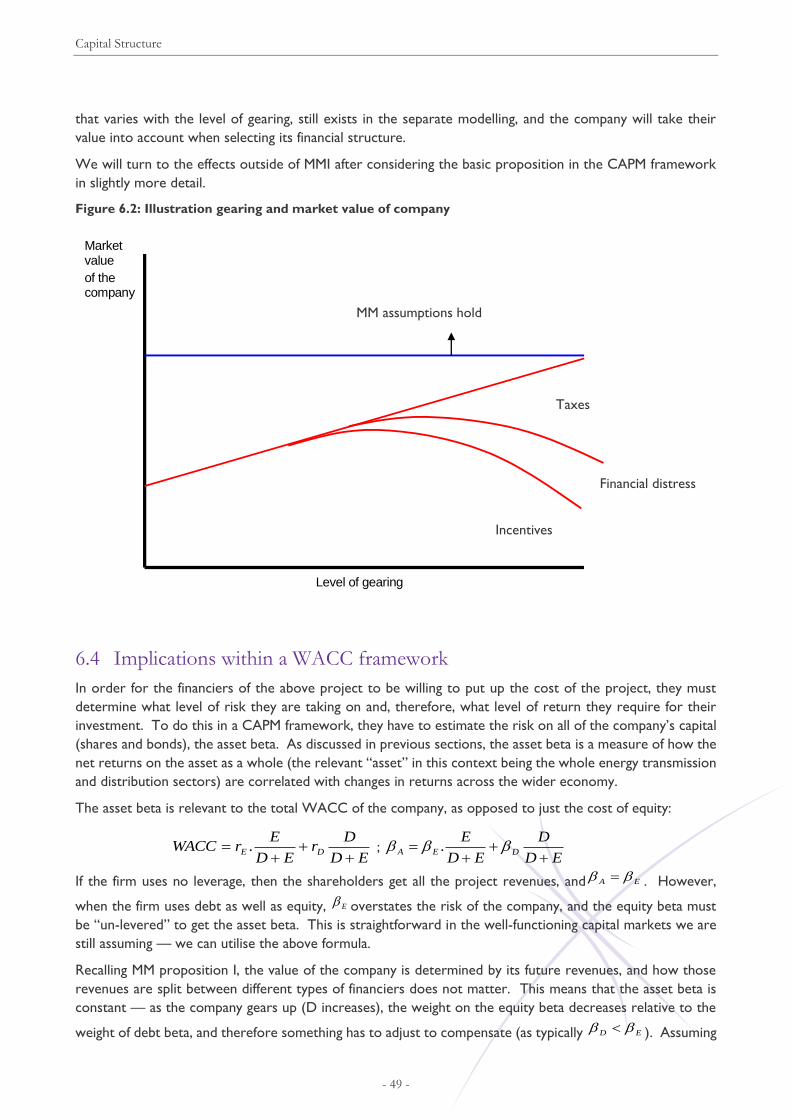
Capital Structure
- 49 -
that varies with the level of gearing, still exists in the separate modelling, and the company will take their
value into account when selecting its financial structure.
We will turn to the effects outside of MMI after considering the basic proposition in the CAPM framework
in slightly more detail.
Figure 6.2: Illustration gearing and market value of company
6.4 Implications within a WACC framework
In order for the financiers of the above project to be willing to put up the cost of the project, they must
determine what level of risk they are taking on and, therefore, what level of return they require for their
investment. To do this in a CAPM framework, they have to estimate the risk on all of the company’s capital
(shares and bonds), the asset beta. As discussed in previous sections, the asset beta is a measure of how the
net returns on the asset as a whole (the relevant “asset” in this context being the whole energy transmission
and distribution sectors) are correlated with changes in returns across the wider economy.
The asset beta is relevant to the total WACC of the company, as opposed to just the cost of equity:
;
If the firm uses no leverage, then the shareholders get all the project revenues, and . However,
when the firm uses debt as well as equity, overstates the risk of the company, and the equity beta must
be “un-levered” to get the asset beta. This is straightforward in the well-functioning capital markets we are
still assuming — we can utilise the above formula.
Recalling MM proposition I, the value of the company is determined by its future revenues, and how those
revenues are split between different types of financiers does not matter. This means that the asset beta is
constant — as the company gears up (D increases), the weight on the equity beta decreases relative to the
weight of debt beta, and therefore something has to adjust to compensate (as typically ). Assuming
Level of gearing
Market value
of the company
MM assumptions hold
Taxes
Incentives
Financial distress
ED
Dr
ED
ErWACC DE
.
ED
D
ED
EDEA
.
EA
E
ED

Capital Structure
- 50 -
that the risk on the debt providers does not change, the risk on equity holders must increase. This in fact is
the case; the risk on the firm’s equity is affected by its capital structure as well as the riskiness of the underlying
business.34
We have now illustrated MMI in the CAPM framework. In perfect capital markets, the fact that a company
gears up does not matter because the risk on equity rises in proportion to exactly compensate, leaving the
asset beta, and therefore the company WACC, unaffected. In fact, it is the asset beta that drives the level of
equity and debt betas — the overall risk on the asset base is what matters, the cost of equity and debt only
adjust to reflect this depending on their relative amounts.
However, things are not as clear as we relax the assumptions behind MMI. The most clear-cut effects are
those associated with taxation, which can be directly analysed in the CAPM framework, and to which we
now turn.
6.4.1 Value of tax shield in CAPM
Bringing taxation into the picture, it is now possible that a company’s value is affected by its capital structure
due to the tax advantage enjoyed by debt finance under many tax regimes — in many countries interest
payments are tax deductible, whereas dividends and capital gains are not.
Roughly speaking, the impact of a change in the level of gearing on the WACC due to the change in the tax
shield value could therefore be calculated as follows. First, estimate the values of the debt and the equity
beta for the previous level of gearing, and using them construct the asset beta. Also remember that as gearing
increases, the company value might be affected by the factors described in paragraph 6.3.1, such that the
trade-offs imply that an increase in gearing would not be desirable above a certain point.
Second, remember that the asset beta will change only as a result of the change in the present value of the
tax shield due to gearing up, which would have to be projected throughout the regulatory price review
period. If there is no additional value from the tax shield compared to current gearing (i.e. current gearing
is optimal), the asset beta can either only stay the same or increase, leading to a fall in the company valuation
(as, other things being the same, the discount rate on the future income is now higher).
Aiming for an “optimal capital structure” implies equating the marginal benefit of debt financing with its
marginal cost. Optimal gearing ratios are likely to vary by sector and even, in principle, by company within
each sector.
6.5 Regulatory precedent
In PR3 we advised the CER for a gearing range of 50 to 60 per cent with a point estimate of 55 per cent; this
was retained in the Mid-Term review. Notional gearing estimates from other regulatory determinations in
the UK and Ireland are presented in the table below.
34 Occasionally, studies are produced in which the cost of equity appears to be invariant to issuance of new debt, with
the argument offered that this is incompatible with MMI. But that is not correct — for example, something happening
to reduce the company’s cost of capital (e.g. greater certainty over its future revenue stream) might naturally be
associated with a decision to issue additional (“securitising” those future revenue streams). It might well be natural
for the amount of debt issued in such a circumstance to be that amount that leaves the cost equity as it was before
the cost of capital fell. (This is particularly likely if the determinant of the capital structure operates through or has
the effect of placing a cap on the cost of equity — debt issuance would continue until that cap was reached.)

Capital Structure
- 51 -
Table 6.1: Recent regulatory precedent for gearing in the UK and Ireland
Company Ofwat
(2014)
CER
Irish Water
(2014)
ComReg
Eircom
(2014)
CAR
DAA
(2014)
CC
NIE
(2013)
Ofgem
NGET
(2012)
Gearing 62.5% 55% 40% 50% 45% 60%
Source: Various regulatory determinations.
6.6 Companies’ submissions
Both EirGrid and ESBN proposed a 55 per cent notional gearing figure in their submissions.
6.7 Conclusion
We retain a notional gearing figure of 55 per cent for our WACC calculations.

Taxes
- 52 -
7 Taxes
7.1 PR3, Mid-Term Review and stakeholder submissions
At PR3 and at the Mid-Term Review the tax rate was taken as 12.5 per cent. That same rate is
proposed by ESBN and EirGrid for PR4.
7.2 Introduction
This section of the report considers issues relating to taxation and the cost of capital. In particular, we
consider different options for the treatment of taxation, and the potential impact of these options on the
revenues allowed for tax liabilities. We conclude our section with our recommendations.
7.3 Different Options for the Treatment of Taxation
We discuss the options available for the treatment of taxation under two headings:
How allowed revenue is provided to allow for tax liabilities
Treatment of tax benefits from gearing above notional level
7.3.1 How allowed revenue is provided to allow for tax liabilities
There are a number of possible approaches that can be used to provide for tax liabilities within a price
control, including:
a) a pre-tax cost of capital calculated using the statutory rate of tax. This is the simplest approach and was
used in setting the PR3 price control. The revenue provided for tax liabilities under this approach may
be either higher or lower than the company’s actual tax liabilities.
b) a pre-tax cost of capital calculated using an effective tax rate. Under this approach, tax liabilities would
still be allowed for within the WACC, but the uplift to the cost of equity would be determined by an
estimate of the effective tax rate faced by the company over the relevant period.
c) a pre-tax cost of capital using the statutory rate of tax, but with an NPV adjustment (e.g. for the tax
benefit from accelerated capital allowances). This option could be seen as part-way between the above
two options.
d) a vanilla cost of capital with an explicit allowance for tax liabilities provided separately. A number of
regulators use this approach, which treats tax in a similar way to opex.
Approaches (b) and (d) can be seen as presentationally different ways of achieving the same outcome, since
both aim to provide allowed revenues for tax which match actual tax liabilities over the price control period.
Similarly, approach (c) can be seen as an attempt to move from (a) towards (d) by including an adjustment to
align revenues allowed for tax more closely with actual tax liabilities during the price control period. For
example, approach (c) might involve making an approximate adjustment in circumstances where the data
required for full modelling of future tax liabilities is not available and hence it might not be practicable to
implement approaches (b) or (d).
Given the above, we consider that the most useful way to approach the analysis is to compare approaches
(a) and (d) as representing the two main alternatives. Hence, in what follows we compare a pre-tax cost of
capital using the statutory tax rate with the use of a vanilla cost of capital and separate allowance for tax
liabilities.

Taxes
- 53 -
In carrying out this comparison, it is also important to take account of how approach (d) would be
implemented in practice. In particular, (and as also noted in the past by the UK Completion Commissions)
if in the future there is a switch from a using a pre-tax WACC based on the statutory rate to allowing for
actual tax liabilities, then the a regulator should make adjustments related to the pre-funding that companies
have received as a result of the use of the statutory rate in previous years.
We discuss below two key aspects that should be considered when deciding the specific tax regime to adopt.
i.e.:
Treatment of tax benefits from gearing above notional level; and
Timing differences considerations.
7.4 Treatment of tax benefits from gearing above notional level
Another important aspect relates to how the tax benefits of gearing above the notional level assumed in the
WACC should be treated. In particular, there are two issues which arise:
First, if the regulated firm is known to have gearing above the notional level at the time that the price
control is set, how should the tax benefits of this be treated?
Second, if the regulated firm chooses to increase gearing during the price control period, how should the
additional tax benefits from doing this be treated?
Under a pre-tax approach to the cost of capital (using the statutory tax rate), the regulator only takes account
of tax shield on debt at the notional level of gearing. Hence, if the firm obtains further tax benefits from
gearing up above the notional level, then (in the absence of any adjustment mechanism) the firm retains these
benefits.35
In the case of a vanilla WACC with separate allowance for tax, what happens depends on whether the
regulator uses the actual or notional level of gearing in forecasting tax liabilities. If the regulator uses the
notional level of gearing (e.g. for consistency with the WACC and with other aspects of the financial
modelling), then again the firm will retain any tax benefits from having higher gearing than the notional level.
By contrast, if the regulator uses the actual level of gearing in modelling future tax payments, then the tax
benefits of higher gearing will be passed through to customers.
In some cases, regulators have introduced explicit adjustment mechanisms to claw back the benefits from
gearing up above the notional level. Hence, in addition to the choice between a pre-tax WACC based on the
statutory rate and a vanilla WACC with a separate tax allowance, the regulator also has to decide whether
to claw back the tax benefits from gearing above the notional level (either by use of actual gearing in modelling
tax liabilities under the vanilla WACC approach, or through some other adjustment mechanism).
7.5 Timing differences
The difference between the effective tax rate and the statutory tax rate arise because of differences between
depreciation and capital allowances and capitalised interest. Both of these differences can be considered as
‘timing differences’ in that they broadly reverse in the long-run; all other things being equal, at some time in
the future the effective tax rate is likely to be greater than the statutory tax rate, and this benefit to equity
will unwind if the regulated entity continues with the statutory rate. Such timing differences have two
implications:
35 There are a number of important points here regarding who bears the higher costs of financial distress if a company
gears more highly and whether (and if so how) regulators should take account of this. For more detail, see
http://www.caa.co.uk/docs/5/ergdocs/20100129EERegFinance.pdf

Taxes
- 54 -
First, when considering tax issues one needs to look beyond any single price control period. Although
a pre-tax approach may provide more revenue than required to fund actual tax liabilities in one price
control period, to the extent that this is driven by timing differences then the situation is likely to reverse
during some future price control period.
Second, from a regulator’s perspective there is a strong rationale for consistency between regulatory
periods. If the regulator consistently applies the same approach then these timing differences are likely
to balance out in the long run.
Third, if the regulator does switch from a pre-tax approach using the statutory rate to a vanilla WACC
approach, then prima facie there is an argument (from the regulator’s perspective) for an adjustment to
compensate for any historic over- or under-funding of tax liabilities. For example, consider the case of
a company which has been regulated using a pre-tax approach to taxation based on the statutory rate
and which has historically been over-funded for tax liabilities. If the regulator were to switch to a vanilla
WACC approach at the point in time when tax liabilities rise above the allowance provided by use of the
statutory rate, then customers would be losing out since they would effectively have provided pre-funding
for tax without receiving any benefit.
7.6 Companies’ submissions
Both EirGrid and ESBN proposed using the statutory tax rate of 12.5 per cent in their submissions.
7.7 Conclusions
We see no strong advantage in CER switching treatment of tax at this point, whilst noting the complications
and costs of changing. Our main view of substance is that the approaches based upon the headline rate of
tax are conceptually superior to those based upon the effective rate, since they leave the discretion to change
investment incentives across the economy, via tax allowances, with the tax authorities (where they should
lie) instead of with the regulator.
Hence we recommend the CER to continue to calculate the WACC on a pre-tax basis using the statutory
rate of 12.5 per cent.

WACC
- 55 -
8 WACC
8.1 Summary
Our draft estimates for the WACC for PR4, before aiming-up, are set out in the table below:
Table 8.1: Overall WACC before aiming-up
High Low Point
estimate
Risk-free rate 2.10 1.75 1.90
Debt premium 1.15 0.75 1.00
Cost of Debt 3.25 2.50 2.90
ERP 5.00 4.60 4.75
Asset beta 0.44 0.31 0.37
Equity Beta 0.98 0.69 0.82
Cost of equity (post-tax) 6.99 4.92 5.81
Tax rate (%) 12.5 12.5 12.5
Cost of equity (pre-tax) 7.99 5.62 6.63
Gearing 0.55 0.55 0.55
WACC (pre-tax) 5.38 3.90 4.58
8.1.1 Companies’ submissions
Table 8.2: WACC submissions by EirGrid and ESBN
EirGrid Spot
estimate ESBN estimate
Risk-free rate 1.75 2.0
Debt premium 1.75 1.75
Cost of Debt 3.5 3.75
ERP 5.0 4.6
Asset beta 0.40 0.36
Equity Beta 0.9 0.8
Cost of equity (post-tax) 6.25 5.68
Tax rate (%) 12.5 12.5
Cost of equity (pre-tax) 7.14 6.49
Gearing 0.55 0.55
WACC (pre-tax) 5.14 4.98
Source: EirGrid and ESBN submissions.
8.2 The principle of aiming up
Reaching a judgement on the likely “true” value of ESB Networks and EirGrid’s cost of capital over the price
control period is inherently subject to uncertainty. In the light of this, it is important to consider how this
uncertainty itself should be taken into account. In particular, what would be the consequences of either
over-estimating or under-estimating the WACC?

WACC
- 56 -
The consequence of setting the regulatory WACC higher than the market cost of capital is that investors
will receive a windfall gain at the expense of electricity customers, who will pay more than necessary for their
electricity.36
This higher payment by customers would, however, be associated with some partially-offsetting gains.
Orthodox price regulation seeks to duplicate the pricing that would prevail in a competitive market. But
prices being above that level increase the likelihood of new entry, enhancing actual competition and
diminishing the need for regulation. Now, the presence of price regulation implies that the regulated entity
has market power, so opportunities for new entry are very probably less than they would be in a competitive
market. But even if the regulated entity were a well-entrenched monopolist, then as well as the standard
problem of monopoly profits leading to allocative inefficiency37 and x-inefficiencies38, prices being occasionally
above the competitive level may also create incentives to innovate and invest, producing new products and
services.39 The standard theory of price regulation suggests that the dynamic incentive gains from excess
profits are less than the allocative efficiency losses from pricing being above the competitive level, but the
key point for our purposes here is to recognise that the consequences of the price cap being set above the
competitive level are not all one way — there are gains from excessive prices as well as losses, even though
the losses outweigh the gains.
On the other hand, the consequence of setting the regulatory WACC lower than the market cost of capital
are less ambiguously negative. First, when prices are below the competitive level there is inefficiently too
much of the regulated product consumed. Furthermore, at the margin the return that companies make on
new investment projects may not be sufficient to cover the cost of raising finance, thus reducing incentives
for the companies to invest. The impact of this on customers would be mitigated by the fact that companies
might have to invest anyway in order to meet licence conditions. However, if under-estimation of the WACC
were serious companies could face difficulties raising the finance which they need, both in debt and equity
markets.
In addition, the setting of too low a WACC might have the result that any new innovations that required
investment would be under-rewarded, thereby reducing the incentive to engage in such investments. That
might imply customers foregoing the gains, in later years, of new cost-reducing technologies or new ways to
pay bills (say). Work by J.A. Hausman and others suggests that the consumer welfare losses from innovation
foregone as a result of regulation can be quite large.40
While customers might benefit from lower bills in the short run if the WACC is set too low, ultimately they
would be expected to suffer in the long run if investment in the electricity sector does not go ahead. Such
negative consequences could potentially last for years into the future.
Hence, while there are material consequences from both over-estimation and under-estimation of the cost
of capital, we consider that on balance the long-term consequences of under-estimation are worse. This
36 This assumes that all other elements of the price control have been set at an appropriate level. In practice, it is of
course possible that errors in setting one part of the price control may be offset by errors in the opposite direction
made elsewhere in the regulatory settlement. 37 “Allocative inefficiency” here means that there will be consumers who are not purchasing the product whose
willingness to pay would be above the marginal cost of producing the product. 38 “X-inefficiencies” arise when the presence of monopoly profits allows technical inefficiencies to continue in the
production process. An example might be that the monopolist is willing to over-pay for some factor of production (e.g.
a raw material or unionised labour). 39 This is a famous point made by Schumpeter. An innovator will secure an advantage over rivals by being able to
increase demand or sell at a higher price. An innovator that is a monopolist will be able to garner all the gains from
this, whereas an innovator that faces competition may in due course face a me-too innovating rival (a rival that produces
a copy-cat innovation), bidding away the profits of the innovation. 40 See, for example, Hausman, Jerry A., “Valuing the Effect of Regulation on New Services in Telecommunications,”
Brookings Papers on Economic Activity, Microeconomics 1997, pp. 1-54.

WACC
- 57 -
implies that, once one has formed a view about the “true” value of the WACC or its components, one should
aim up to take account of the asymmetry of consequences from getting the decision wrong.
It should be noted, however, that the above discussion of asymmetric consequences does not mean that it is
necessary to be certain that the estimate is not too low — given that estimates of each WACC parameter
are subject to significant uncertainty this might require such a high mark-up that it would not be in consumers’
interests. As an alternative to simply aiming up and leaving the gains with regulated entities, it would be
possible to envisage an alternative mechanism, whereby a regulator aimed up in devising a price control but
then had an ex post review of the realised WACC and clawed back all or some portion of the difference.
That would, however, create a number of complex incentives the analysis of which would take us beyond
our scope here.
The principle that there is an asymmetry of consequences between those of setting the cost of capital too
low and those of setting it too high is now well-established by regulators (and the Competition Commission
in the UK).41 Too high a cost of capital, and consumers today pay a little more than would occur in a
competitive market. Too low a cost of capital, and consumers tomorrow miss out on the benefits of
investment and innovation that does not occur. The latter costs are generally recognised as significantly
exceeding the former. Consequently, Europe Economics recommends that the regulatory cost of capital
should be set above the central estimate of the market cost of capital.
The issue of precisely how much to aim up is debated, as is the issue of whether aiming up should take place
on the basis of the overall WACC or its individual components. In its advice on the Q5 London airports
price control, the Competition Commission aimed up a number of estimated parameters in the WACC
calculation (such as the equity beta) to the 95th percentile.
In our advice to Ofwat in the PR09 water sector review in the UK, Europe Economics argued that the
purpose of aiming up is not to eliminate all possibility that the WACC has been set too low but, rather,
merely to reflect the presence of some asymmetry in the consequences of too low versus too high a value.
We stress that
On this basis we disagreed with what was at that point the position adopted by the UK’s Competition
Commission, where it aimed up to the 95th percentile — i.e. close to two standard deviations from the mean
in a normal distribution, the usual statistical measure of certainty. Instead, we proposed aiming up of the
order of one standard deviation rather than two. More recent regulatory judgements on aiming up have
adopted figures in the 75th-80th percentile range.42
8.3 Regulatory precedent
Choosing a value for the WACC that is above the regulator’s expected value for the WACC has been
standard practice for regulators for many years, across many regulated sectors and in particular in the
communications sector, both in Europe and outside. The process by which this is done has often been
implicit – via the choice of a “conservative” estimate of a particular parameter such as the beta or the equity
risk premium. In other situations it is done by choosing, as a point estimate, a value above the mid-point of
quoted range for the WACC as a whole or some key building block thereof.
Wholly implicit conservativeness is not straightforward to evidence, but the practice of choosing a point
estimate above the mid-point can be seen in a number of determinations. How regulators choose a point
41 For aiming up in Ireland, see the most recent Commission for Energy Regulation decision on electricity transmission
and distribution networks: Commission for Energy Regulation (2014) “Mid-Term review of WACC applying to the
Electricity TSO and TAO and ESB Networks Ltd for 2014 to 2015”, CER/14/026. 42 For example, see the UK Civil Aviation Authority’s 2013 Q6 price control proposals.
WACC
- 58 -
estimate from within a range was explored by the consultancy “Economic Insights” in a recent (June 2014)
report for the New Zealand Commerce Commission.43 Of 53 decisions reviewed in that document, 35
involved choices of the point determination of the WACC at above the mid-point of the quoted range. The
authors remarked that, for those cases where the point estimate used of the WACC is not explicitly above
the mid-point of the range, “This often reflects adopting a conservative view of the market risk premium and
equity beta that are used in the Capital Asset Pricing Model (CAPM) for determining the return on equity,
where ‘conservative’ means erring on the high side.”44
We note that the point estimates we have provided are, in our view, our best estimates of true forward
looking values and do not represent a conservative representation. As explained above, aiming-up on our
WACC estimate is best dealt with separately and in a transparent manner.
In both PR3 and the Mid-Term WACC review, our final WACC recommendation included some degree of
aiming-up. We stress that, in the context of PR4, the degree of uncertainty in the WACC is less than at the
Mid-Term WACC review (as noted in that review, the degree of aiming-up was amplified by the Mid-Term
nature of the review and the risk that firms had under-recovered in 2011 and 2012) and potentially also less
than at PR3.
The justification for such conservativeness was set out by the UK regulator Ofcom in a 2005 methodological
paper.45 Ofcom stated:
“Traditionally, Ofcom has considered that the downside risk associated with taking too
low a value for the ERP (discouraging discretionary investment) is more detrimental to
the interests of consumers than taking too high a value (leading to higher prices to
customers) and has tended to the higher end of the possible range. Having reviewed its
approach in this area, Ofcom remains of this view”.
This methodological position was confirmed in its Final Statement of August 2005.46
8.4 Recommended WACC range and aimed-up point WACC
Our recommendation for the degree of aiming up is based upon a Monte Carlo analysis using
The ranges recommended for each building block of the WACC.
An assumption of a uniform distribution of outcomes across each range.
1000 runs.
Calculation of the standard deviation of outcomes across the runs.
Application of one standard deviation as the level of aiming up to be applied to our preferred point
estimate.
Construction of the recommended range as running from one standard deviation below the best estimate
to two standard deviations above it.
43 Economic Insights (2014) “Regulatory precedents for setting the WACC within a range”. 44 Economic Insights (2014) “Regulatory precedents for setting the WACC within a range”, p. iii. 45 Ofcom (2005) “Ofcom's approach to risk in the assessment of the cost of capital”. See paragraphs 1.13, 4.28, and
4.33 of http://stakeholders.ofcom.org.uk/binaries/consultations/cost_capital/summary/cost_capital.pdf. 46 Ofcom (2005) “Ofcom’s approach to risk in the assessment of the cost of capital”. See paragraph 4.73 of
http://stakeholders.ofcom.org.uk/binaries/consultations/cost_capital2/statement/final.pdf. Note also that at
paragraph 4.33 Ofcom again confirms that it picks points above the mid-point of its ranges: “By proposing values
that are towards the upper end of a reasonable range…”.

WACC
- 59 -
The result is that the standard deviation is 0.2 percentage points, implying a recommended WACC range of
4.4 to 5.0 per cent, and producing an overall pre-tax WACC point recommendation, after aiming up, of 4.8
per cent.
8.5 Inflation
We base our range on forecasts for CPI and HICP inflation over the coming years. Our HICP forecast was
obtained from the Irish budget report for 2015 and was provided by the department of finance while our CPI
forecasts were obtained from PWC’s “Global Economy Watch” economic projections section. These
forecasts are presented below.
Table 8.3: Inflation
Inflation
measure 2015 2016 2017 2018
HICP 1.1% 1.4% 1.4% 1.4%
CPI 0.8% 1.1% 1.5% 1.5% Source: PWC Global Economy Watch and http://www.budget.gov.ie/Budgets/2015/2015.aspx.
Based on these forecasts our point estimate for inflation is 1 per cent for 2015 and 1.4 per cent for 2016
onwards.

Financeability
- 60 -
9 Financeability
9.1 Role of financeability
Financeability analysis has three main potential objectives:
1. It provides a consistency check. The WACC calculation involves an assumed level of gearing and assumed
credit rating. If that level of gearing is not consistent with the achieving of that credit rating, that should
be exposed by the financeability analysis.
2. Some regulators have the statutory duty to ensure that regulated entities are able to finance their
functions. In such cases, financeability analysis tests whether this duty can be met.
3. WACC calculations, along with other elements of the price control, are based upon an assessment of a
notional entity and of the actual regulated entities’ capacity to enhance efficiency (operating and financial).
The financeability test can be used to provide an analysis of how much is being asked of the actual entity.
For our purposes here, we focus upon objective 1 — consistency with the target credit rating.
9.2 ESB Financeability: indicative analysis
We next set out a preliminary view of ESB’s financeability. Specifically, we discuss the following:
The target credit rating.
The financial ratios that are the most relevant ones to focus on.
What numbers one should expect for these financial ratios in order to achieve the target credit rating.
The projected financial ratios given ESB’s forecast expenditure, and what this implies for the financeability
of ESB.
It should be noted that the quantitative assessment here is based on ESB’s forecast expenditure for the
forthcoming price control period for the distribution network and the transmission network. This analysis
would need to be revisited in the light of the CER’s view on what costs will be allowed in the next price
control period.
As regards EirGrid, we provide a separate note in which we consider the applicability of the RAB-WACC
approach to EirGrid.
9.2.1 Actual vs target credit ratings
The first question is what target credit rating should be assumed in the analysis. ESB currently achieves the
following credit ratings47:
Standard & Poor's: BBB+ (stable).
Moody's: Baa1 (Stable).
Fitch: BBB+ (stable).
We note that these credit ratings are consistent with the “comfortable investment grade” (i.e. at investment
grade, BBB, and sufficiently at or above that rating that the investment grade rating can be regarded as secure
and comfortable — usually interpreted as at least one step above, i.e. BBB+ or higher) that we adopt as the
target credit rating for the purposes of estimating the debt premium.
47 http://www.esb.ie/main/about-esb/credit-ratings.jsp.

Financeability
- 61 -
9.2.2 Most relevant financial ratios
ESB is rated by Standard and Poor’s, Moody’s and Fitch, and hence ideally the financeability analysis would
cover the financial ratios used by all three ratings agencies. The full list of relevant financial ratios is as follows:
Net debt / RAV
FFO interest cover
Post-maintenance interest cover ratio (PMICR), also known as “adjusted interest cover ratio”
FFO / net debt
Retained cash flow (RCF) / capex
The table below shows which of the ratings agencies uses which of these ratios:
Table 9.1: Financial ratios used by different rating agencies
Fitch Moody’s Standard & Poor’s
Net debt / RAV (%) FFO interest cover (x) PMICR (x)
FFO / net debt (%) RCF / Capex (x)
Source: Ofgem, “Strategy decision for the RIIO-EDI electricity distribution price control – Financial issues”, 4 March 2013,
https://www.ofgem.gov.uk/ofgem-publications/47071/riioed1decfinancialissues.pdf (page 26).
The financial models which the CER has sent us calculate all of these ratios except for PMICR.48 Hence, in
the analysis which follows we consider:
Net debt / RAV;
FFO interest cover;
FFO / net debt; and
RCF / capex.
9.2.3 What numbers one should expect for these financial ratios
Below we present a table (extracted from the same recent document published by Ofgem referenced above)
of the financial ratios associated with different credit ratings.
Table 9.2: Financial ratios associated with different credit ratings
Fitch Moody’s Standard & Poor’s
A BBB A Baa A BBB
Net debt / RAV (%) 50 – 65 >65 45 – 60 60 – 75 <70 >70
FFO interest cover (x) 4.0 – 5.0 <4.0 3.5 – 5.0 2.5 – 3.5 >3.5 2.5 – 3.5
PMICR (x) >1.7 <1.7 2.0 – 4.0 1.4 – 2.0
FFO / net debt (%) 12 – 20 8 – 12 >12 8 – 12
RCF / Capex (x) 1.5 – 2.5 1.0 – 1.5 Source: Ofgem, “Strategy decision for the RIIO-EDI electricity distribution price control – Financial issues”, 4 March 2013,
https://www.ofgem.gov.uk/ofgem-publications/47071/riioed1decfinancialissues.pdf (page 26)
We emphasise the importance of noting that the above table relates to category ratings – in other words,
“BBB” refers to the BBB category, covering BBB+, BBB and BBB-. This is important, because it implies that
ESB’s financial ratios might need to be at the upper end of the range quoted by Standard and Poor’s for the
BBB category in order to achieve a target rating of BBB+ (though it is unclear what precisely secures a “+”
or “-“ qualification — in principle that could also, perhaps, be associated with a firm that squeaks in on the
48 The full list of financial ratios calculated by the CER’s financial model is: EBIT interest cover; EBITDA interest cover;
Net Debt/RAV; EBITDA/net debt; operating cashflows/capex; FFO interest cover; FFO/net debt; retained cash
flow/net debt; retained cash flow/capex.

Financeability
- 62 -
ratios but seems very unlikely to have them fall). (We note as well that these metrics are for the UK – we
have not at this stage considered it proportionate to investigate to what extent ratings agencies expect
different ratios from companies in Ireland. That additional step will become proportionate and be pursued
once we have access to a full financial model that allows for a full financeability analysis.)
The table below shows the financial metric thresholds used by Ofgem in July 2014 in the draft determinations
for the RIIO-ED1 price review.
Table 9.3: Financial metric thresholds used by Ofgem
Financial metric Threshold
Key ratios identified above
FFO interest cover ratio 2.5 min
FFO/ Net Debt 8% min
Net Debt / RAV 80% max
RCF / Capex 0.5 min
Other ratios monitored by Ofgem
Adjusted interest cover ratio, or PMICR 1.4 min
RCF / Net Debt 5% min
Regulated equity / EBITDA 5.5 max
Regulated equity / PAT 18 max
Dividend cover ratio 1.0 min Source: Ofgem, “RIIO-ED1: Draft determinations for the slow track electricity distribution companies, Financial Issues, Supplementary annex to RIIO-
ED1 overview paper”, 30 July 2014, https://www.ofgem.gov.uk/ofgem-publications/89072/riio-ed1draftdeterminationfinancialissues.pdf.
For our indicative purposes here, and noting again that we do not at this stage have access to a financial
model (including the CER’s assessment of allowed costs) that would allow a more complete analysis, we
proceed for now on the basis that it is appropriate to use the same ratios that Ofgem used in the UK.
9.2.4 Projected financial ratios
An important question is whether financeability testing should be applied at the level of each licensed entity
(implying separate financeability testing for transmission and for distribution) or at the level of the group as
a whole. We recognise that there may be pragmatic arguments in favour of doing the financeability testing
at a group level, on the assumption that this is the level at which ESB will issue debt. On the other hand,
however, it can be argued that it is more correct theoretically to test financeability at the level of each
licensed entity, since price regulation is intended to allow each licensed entity to finance its functions as a
stand-alone entity.
Assessment of financial ratios at a group level could potentially mask financeability problems in any one
business. In what follows, we therefore consider the distribution and transmission businesses separately.
The table below summarises the financial ratios calculated on the basis of ESB’s forecast cash flows for the
distribution network and for the transmission network.
Table 9.4: Financial ratios calculated on the basis of ESB’s forecast cash flows
DSO TAO Target
Average for 2016-20 Average for 2016-20
Net debt / RAV (%) 52% 46% 80% max
FFO interest cover (x) 4.7 7.8 2.5 min
FFO / net debt (%) 15% 15% 8% min
RCF / Capex (x) 1.3 0.6 0.5 min

Financeability
- 63 -
9.2.5 Conclusion
As can be seen, if all of ESB’s expenditure was allowed (as forecast), its cash flows would not pose any
financeability concerns. Accordingly, at this stage we conclude that this provisional, high-level financeability
analysis suggests that the WACC proposed is compatible with the comfortable investment grade credit rating
recommended.
We note that ESBN has sought a higher credit rating than we have assessed here. We believe the target
here to be the correct one, for the reasons set out in our cost of debt analysis section above. But we observe
that, if ESBN were subject to a higher credit rating, then its debt premium would be expected to fall (higher
credit ratings mean lower debt premia, ceteris paribus). So its actual cost of capital would fall. But if achieving
that credit rating meant it failed the financeability analysis, then (absent other remedies such as demanding a
lower gearing level) one option to restore financeability would be the crude one of permitting higher prices
and thus higher returns. In that case, allowing ESBN a higher assumed credit rating would simultaneously
reduce its cost of capital and increase its rate of return — meaning the benefits of that lower cost of capital
would all accrue to the firm, with consumers losing out through higher prices.