Retrospective Theses and Dissertations Iowa State University Capstones, Theses andDissertations

1998

Power system security boundary visualization usingintelligent techniquesGuozhong ZhouIowa State University

Follow this and additional works at: https://lib.dr.iastate.edu/rtd

Part of the Artificial Intelligence and Robotics Commons, and the Electrical and ElectronicsCommons

This Dissertation is brought to you for free and open access by the Iowa State University Capstones, Theses and Dissertations at Iowa State UniversityDigital Repository. It has been accepted for inclusion in Retrospective Theses and Dissertations by an authorized administrator of Iowa State UniversityDigital Repository. For more information, please contact digirep@iastate.edu.

Recommended CitationZhou, Guozhong, "Power system security boundary visualization using intelligent techniques " (1998). Retrospective Theses andDissertations. 11904.https://lib.dr.iastate.edu/rtd/11904

INFORMATION TO USERS

This manuscript has been reproduced from the microfihn master. UMI

films the text directly from the original or copy submitted. Thus, some

thesis and dissertation copies are in typewriter &ce, while others may be

fix>m any type of computer printer.

The quality of this reproduction is dependent upon the quality of the

copy submitted. Broken or indistinct print, colored or poor quality

illustrations and photographs, print bleedthrough, substandard mar^ns,

and improper alignment can adversely affect reproductioa

In the unlikely event that the author did not send UMI a complete

manuscript and there are missing pages, these will be noted. Also, if

unauthorized copyright material had to be removed, a note will indicate

the deletion.

Oversize materials (e.g., maps, drawings, charts) are reproduced by

sectioning the original, b^inning at the upper left-hand comer and

continuing from left to right in equal sections with small overiaps. Each

original is also photographed in one exposure and is included in reduced

form at the back of the book.

Photographs included in the original manuscript have been reproduced

xerographically in this copy. Higher quality 6" x 9" black and iniiite

photognq)hic prints are available for any photographs or illustrations

appearing in this copy for an additional charge. Contact UMI directly to

order.

UMI A Bdl & Howdl Infimnation Conqany

300 North Zeeb Road, Ann Aibor MI 48106-1346 USA 313/761-4700 800/521-0600

Power system security boimdary visualization using intelligent techniques

by

Guozhong Zhou

A dissertation submitted to the graduate faculty

in partial fulfillment of the requirements for the degree of

DOCTOR OF PHILOSOPHY

Major: Electrical Engineering (Electric Power)

Major Professor: James D. McCalley

Iowa State University

Ames, Iowa

1998

Copyright © Guozhong Zhou, 1998. All rights reserved.

Xnn Number: 9841100

UMI Microform 9841100 Copyright 1998, by UMI Company. All rights reserved.

This microform edition is protected against unauthorized copyii under Title 17, United States Code.

UMI 300 North Zeeb Road Ann Arbor, MI 48103

ii

Graduate College Iowa State University

This is to certify that the Doctoral dissertation of

Guozhong Zhou

has met the dissertation requirements of Iowa State Uni\-ersity

Major Professor

For the Major Program

College

Signature was redacted for privacy.

Signature was redacted for privacy.

Signature was redacted for privacy.

Ill

TABLE OF CONTENTS

INTRODUCTION 1

1.1 Motivation for security boundar\- visualization 1

1.2 Traditional security boundarj' visualization approach 2

1.3 Automatic security boundar\- visualization methodology- 4

1.4 Sample system .5

1.4.1 Thermal overload 6

1.4.2 \bltage instability 7

1.5 Contributions of this dissertation 8

1.5.1 Development of a systematic data generation method 8

1.5.2 Development of an efficient feature selection tool for operating

parameter selection 8

1.5.3 Application of data analysis techniques for neural network training 9

1.5.4 Confidence interval calculation for neural network performance

evaluation 9

1.5.5 Sensitivity analysis of neural network outputs with respect to inputs 9

1.5.6 Development of a composite boundar>' visualization algorithm . . 9

1.5.7 A\-ailabIe transfer capability calculation based on the boimdarv* . 10

1.6 Organization of this dissertation 10

LITERATURE REVIEW 11

2.1 Introduction 11

IV

2.2 Neural network applications to security assessment 12

2.3 Problems related to neural network applications 13

2.4 Other intelligent technique applications to security assessment 13

2.5 Another approach - security assessment via boundar\' visualization .... 14

3 DATA GENERATION AND DATA ANALYSIS 16

3.1 Introduction 16

3.2 Data generation 16

3.2.1 Overview 17

3.2.2 Data preparation 20

3.2.3 Boundarv' search 23

3.2.4 Revised Latin hypercube sampling 25

3.2.5 Data generation for the sample system 28

3.3 Data analysis 29

3.3.1 Techniques for outlier detection 29

3.3.2 Techniques for outlier detection and distribution visualization . . 42

3.4 Summarj- 44

4 FEATURE SELECTION 54

4.1 Introduction 54

4.2 Literature overview 55

4.3 Critical parameter candidates for the sample system 56

4.4 Statistical method - Cluster analysis 56

4.5 Neural network method - Kohonen self-organizing map 59

4.6 Genetic algorithm method 61

4.6.1 Design of GANN 62

4.6.2 Application to the sample system 64

4.6.3 Improvement on solution speed 68

V

4.7 Comparisons of different feature selection methods 76

4.7.1 Solution speed 77

4.7.2 Prediction accuracy 77

4.8 Summar}' 78

5 TRAINING AND USING NEURAL NETWORKS FOR BOUND­

ARY APPROXIMATION 79

5.1 Introduction 79

5.2 Training neural networks 79

5.2.1 Overntting and underfitting 79

5.2.2 Exploration of improvement on accuracy near the boundar\- ... 80

5.3 Confidence intervals for neural network outputs 82

5.4 Sensitivity analysis of the neural network output with respect to input

parameters 88

5.5 Summar\' 90

6 PRESENTATION TECHNIQUES 92

6.1 Introduction 92

6.2 Problem formulation 92

6.3 Individual boundarv- visualization 94

6.3.1 General description 94

6.3.2 Application to the thermal overload problem 95

6.3.3 Application to the voltage instability problem 99

6.3.4 Choice of presented parameters by users 106

6.4 Composite boundarj- visualization 106

6.4.1 Conceptual Formulation 106

6.4.2 Algorithm Description 109

6.4.3 Applications to the sample sj'stem 110

v-i

6.5 Available transfer capability calculation 114

6.6 Obtaining update functions 115

6.7 Summary' 116

7 CONCLUSIONS AND FURTHER WORK 117

7.1 Conclusions 117

7.2 Further work 119

BIBLIOGRAPHY 121

ACKNOWLEDGMENTS 132

vii

LIST OF TABLES

Table 3.1 The structure of a KEEP file 18

Table 4.1 Critical parameter candidates for the thermal overload and volt­

age instability problems .56

Table 4.2 Nodes on the map with their associated attributes for the thermal

overload problem 61

Table 4.3 Feature selection results for the line thermal overload with car­

dinality levels 5-10 (using MLPs) 65

Table 4.4 Feature selection results for the voltage instability with cardinal­

ity levels 9-13 (using MLPs) 67

Table 4.5 Feature selection results for the thermal overload with cardinality

levels 5-10 (using RBFXs) 74

Table 4.6 Comparison of feature selection results using RBFXs and KXXs

for the thermal overload problem 76

Table 4.7 Comparison of solution time (s) 77

Table 4.8 Comparison of prediction accuracy 78

Table 6.1 Results of thermal overload boundary accuracy assessment ... 96

Table 6.2 Test results for ASAS generated operating conditions 100

Table 6.2 (continued) 101

Table 6.3 Initial operating condition for line thermal overload and trans­

former overload Ill

Vlll

Table 6.4 Initial operating condition for voltage instability

ix

LIST OF FIGURES

Figure 1.1 Nomogram curves for three critical parameters 3

Figure 1.2 Procedure for security boundarv' visualization 4

Figure 1.3 A sample system 6

Figure 3.1 Automatic security assessment software package 18

Figure 3.2 Uniform sampling in two dimensions 26

Figure 3.3 Revised Latin hypercube sampling in two dimensions 27

Figure 3.4 Accumulative v-ariation of principal components for the thermal

overload problem 32

Figure 3.5 Accumulative variation of principal components for the voltage

instability problem 33

Figure 3.6 The first two principal components for the thermal overload prob­

lem with the original data set .33

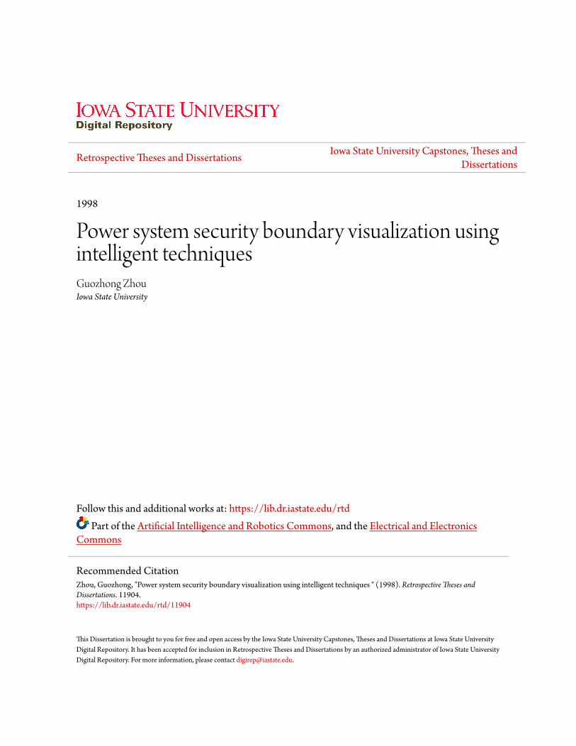
Figure 3.7 The last two principal components for the thermal overload prob­

lem with the original data set 34

Figure 3.8 The first two principal components for the thermal overload prob­

lem with the altered data set 34

Figure 3.9 The last two principal components for the thermal overload prob­

lem with the altered data set 35

Figure 3.10 Error versus density in training data 37

Figure 3.11 Plot of D f ' s for the thermal overload data set with 1,005 samples 39

X

Figure 3.12 Q-Q plot of Vi and u, for the thermal overload data set with 1.005

samples 40

Figure 3.13 Q-Q plot of f, and Uj for the thermal overload data set with 1.004

samples (sample 265 removed) 40

Figure 3.14 Organization of a Kohonen self-organizing map for the thermal

overload problem 46

Figure 3.15 Organization of a Kohonen self-organizing map for the voltage

instability problem 46

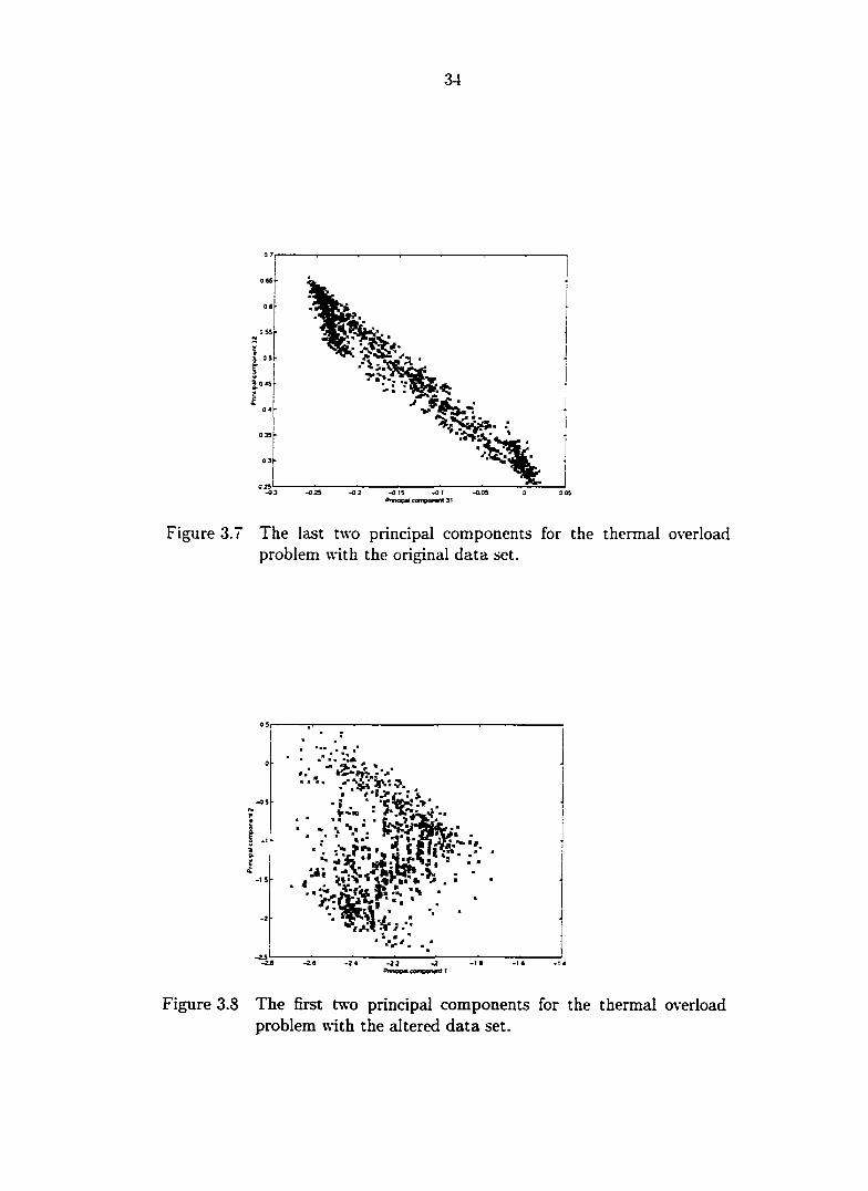
Figure 3.16 Attribute 18 (voltage magnitude) for the thermal overload problem. 47

Figure 3.17 Attribute 19 (voltage magnitude) for the thermal overload problem. 47

Figure 3.18 Attribute 17 (line flow) versus subarea load for the thermal over­

load problem 48

Figure 3.19 Voltage magnitude 7 versus subarea load for the thermal overload

problem 48

Figure 3.20 Voltage magnitude 9 versus subarea load for the thermal overload

problem 49

Figure 3.21 Generation A versus subarea load for the thermal overload problem. 49

Figure 3.22 A trajector}' 50

Figure 3.23 A view of data for the thermal overload problem with the original

data set 50

Figure 3.24 A view of data for the thermal overload problem with the original

data set 51

Figure 3.25 A \iew of data for the thermal overload problem with the original

data set 51

Figure 3.26 A \iew of data for the thermal overload problem with the altered

data set 52

xi

Figure 3.27 A view of data for the thermal overload problem with the altered

data set 52

Figure 3.28 A view of data for the thermal overload problem with the altered

data set 53

Figure 3.29 A view of data for the voltage instability problem 53

Figure 4.1 Cluster tree for the data set of the thermal overload problem . . 58

Figure 4.2 Cluster tree for the data set of the voltage instability problem . . 59

Figure 4.3 A 4x4 organized map of attributes for the thermal overload prob­

lem 60

Figure 4.4 A 4x4 organized map of attributes for the voltage instability

problem 60

Figure 4.5 Basic functional structure of GANN 62

Figure 4.6 A radial basis function network 69

Figure 4.7 A radial basis function in one-dimensional space 69

Figure 4.8 A portion of two-dimensional feature space covered by RBFs . . 70

Figure 4.9 Test errors versus number of centers (random selection of centers) 75

Figure 4.10 CPU time versus number of centers (random selection of centers) 75

Figure 5.1 Variation of training and test errors with the number of iterations. 81

Figure 5.2 Plot of function a- = 1 — 82

Figure 5.3 R values for the test samples 83

Figure 5.4 Test error distributions 83

Figure 5.5 A detailed structure of a multilayer perceptron 86

Figure 5.6 90% confidence interval for the test data of the thermal overload

problem 88

Figure 5.7 Sensitivity of the MLP output with respect to the 8 input pa­

rameters for the thermal overload problem 89

xii

Figure 5.8 Sensitinty of the MLP output with respect to the 11 input pa­

rameters for the voltage instability problem 90

Figure 6.1 Thermal overload boundary- for initial points 1:0 and 2:0 97

Figure 6.2 Thermal overload boundarv- for initial points .3:0 and 4:0 97

Figure 6.3 Thermal overload boundary- for initial points 5:0 and 6:0 98

Figure 6.4 Thermal overload boundar\- for initial points 7:0 and 8:0 98

Figure 6.5 \bltage instability boundary- for initial points 9:0 and 10:0 .... 102

Figure 6.6 Voltage instability boundar\'for initial points 11:0 and 12:0 . . . 102

Figure 6.7 \bltage instability boundar>- for initial points 13:0 and 14:0 . . . 103

Figure 6.8 \'oltage instability boundar>- for initial points 15:0 and 16:0 . . . 103

Figure 6.9 A boundar\- with presented parameters Generation A and Gen­

eration B 106

Figure 6.10 A boundarv- with presented parameters Generation A and Gen­

eration C 107

Figure 6.11 A boundar>' with presented parameters Generation B and Sub-

area Load 107

Figure 6.12 A boundar\- with presented parameters Generation C and Sub-

area Load 108

Figure 6.13 A composite boundary- formed by individual boundaries 109

Figure 6.14 Illustration of the algorithm to determine the composite boundan,-. Ill

Figure 6.15 Line thermal overload boundary-. 112

Figure 6.16 Transformer overload boundar\-. 112

Figure 6.17 Voltage instability boundary-- 113

Figure 6.18 Composite boundary for line thermal overload, transformer over­

load, and voltage instability problems 113

Figure 6.19 The ATC calculation illustration 114

1

1 INTRODUCTION

1.1 Motivation for security boundary visualization

In the open access environment, utilities face a number of challenges to be more

competitive. One of these challenges is that typical operating conditions tend to be

much closer to security boundaries. This is because transmission utilization is increasing

in sudden and unpredictable directions, and competition together with other regulators-

requirements make new transmission facility construction more difficult. Consequently,

security levels for the transmission network must be accurate and easily identified on-line

by system operators.

Power system security assessment can be divided into two levels: classification and

boundary' determination. Classification involves determining whether the system is se­

cure or insecure under all prespecified contingencies. The sv'stem is secure if the post-

contingency performance is acceptable. Classification does not in itself indicate distance

from the operating condition to the insecure conditions. Boundeirj* determination, on

the other hand, involves quantifving this distance. A boundary- is represented by con­

straints imposed on parameters characterizing precontingency conditions. These pre-

contingency parameters are called critical parameters. Once the boundar>- is identified,

security assessment for any operating point can be given as the distance (in terms of

critical parameters) between the current operating point and the boundarv'. Assess­

ment in terms of precontingency operating parameters instead of the postcontingency

performance measure is more meaningful to the operator.

2

1.2 Traditional security boundary visualization approach

In many North American utilities, the traditional boundar\- characterization ap­

proach is used to generate a two-dimensional graph called a nomogram [1] - [3]. of

which two axes correspond to two critical parameters. To develop a nomogram, two

critical parameters are chosen and all other critical parameters are set to selected values

within a typical operating range. The noncritical parameters, which may influence the

postcontingency performance measure, are set to constant values biased to be conserva­

tive with respect to the influence on the performance measure. Points on the nomogram

curve are determined by repeating computer simulations. var\-ing one critical parameter

while keeping the other constant. If the relationship between the performance measure

and the critical parameters is fairly linear, interpolation and/or extrapolation helps to

obtain boundary' points. In this case, only three or four simulations may be needed.

But highly nonlinear relationships may require more simulations. The above procedure

is repeated for selected values of the first critical parameter provides enough boundary-

points to draw the nomogram curve. In the case where there is a third critical pa­

rameter value change, a different nomogram curve is drawn for each value of this third

critical parameter so that the result is a family of nomogram curves, as illustrated in

Figure 1.1. Inclusion of a fourth critical parameter value change requires a distinct

family of nomogram curves (i.e., a new page) for each new \-alue of the fourth critical

parameter. Inclusion of fifth critical parameter value change requires a distinct family

of pages for each new \^ue of the fifth critical parameter, and so on. Ob\iously. the

above manual approach requires intensive labor involvement. The other disadvantages

include inaccurate boundary representation and little flexibility to integrate with the

energy management sj'stem (EMS).

There are two main approximations made in nomogram development which can ul­

timately result in inaccurate boundary characterization when the nomogram is used by

Figure 1.1 Xomogram curves for three critical parameters

the operator. One is linear interpolation between points. The other is insufficient infor­

mation contained in critical parameters. Because of labor requirements, the simulation

procedure described above is normally used to obtain only a ver\' few points on the

boundar\-; indeed, often only the "comer points" are obtained. The remaining portions

of the boundar>- are obtained by drawing a straight line through the computed points.

This approximation can be improved by automating the security assessment process so

that the number of points generated is only limited by computer availability, and by

using neural networks, an interpolation tool that models ver\- well nonlinear portions of

the boundarj-. As for the second approximation, nomogram development usually limits

the number of critical parameters to five or less, even when there are other parameters

knowTi to be influential. There are two reasons for this. First, having more critical

parameters requires performing more simulations. Second, it is difficult to compactly

represent the information to the operator if there are more than five critical parameters.

For example, if the fourth and fifth parameters have six different levels of interest, the

operator would require 36 pages of three parcimater nomogram curves. Limiting the

number of critical paramaters may mean that the information content of the parameters

that are used is insufficient for accurately predicting the performance measure. The

approximation due to insufficient information contained in critical parameters can be

improved by automatically performing a large number of simulations with little atten­

4

tion from the analyst, and by using neural networks that provide compact boundar\-

characterization for any number of critical parameters. The difficulty in integrating the

procedure into the EMS lies in the manual nature of the traditional approach. This can

be solved by using an automatic approach.

Therefore, to overcome the disadvantages of the traditional approach, an automatic

security boundar>' visualization methodology- has been developed using intelligent tech­

niques [4] - [8].

1.3 Automatic security boundary visualization methodology

As Figure 1.2 shows, the procedure developed in this dissertation to determine and

illustrate security boundaries includes six steps.

r Step I Step 2 Step 3 Step 4

Identify Security Problem

Construct Basecase DATA GENERATION

(AulonuDc secunty

assessment software)

J KEEP\ •7 HLE r

(Large database 1/

FEATURE SELECTION

(Genetic algorithm based t'eature selection)

vy

Step 6 Step 5 1

NEURAL NETWORK

VISUAUZATION

WEncodedV Input/ 1 output 1

\ relation/

TRAINING

J

Figure 1.2 Procedure for security boundary- visualization

1. Security problem identification: This step is no different from what is done when

generating nomograms in the traditional, manual way. Therefore, it is a task of

the engineer to identify- the specific set of security constraints to be characterized

and candidate operating parameters that may have influence on these constraints.

5

2. Base case construction: This is also much like what is done in the traditional way.

A base case power flow solution needs to be constructed that appropriately models

the system conditions of concern.

3. Data generation: This step involves an automated procedure that generates a large

database, with each record consisting of precontingency operating parameters and

the corresponding postcontingency performance measure.

4. Feature selection: This step selects the best subset of precontingency operating

parameters for use in predicting the postcontingency performance measure.

5. Neural network training: Based on the selected parameters and the data base

obtained from previous steps, this step perform neural network training for function

approximation of the mapping from the precontingency operating parameters to

the postcontingency performance meaisure.

6. Visualization and presentation: This step integrates the encoded neural network

mapping into a visualization software that can be used on-line to generate the

security boundarv-.

Although it is assumed in this dissertation that steps 1 to 5 are performed off-line,

it is expected that our development of these steps will ultimately be applicable on-line.

1.4 Scimple system

A sample sv'stem is shown in Figure 1.3. This is just a simplified illustration of a

real system, a 2500-bus model of Northern California. The detailed sj-stem is used for

all simulations throughout this research. This 2500-bus nodel will be used for testing

all studies conducted in this dissertation. The load in the subarea, diuing high loading

6

conditions, is greater than the generation capacity in the subarea. Therefore, a signifi­

cant amount of power must be imported into the subarea to meet the demand. There

are several ties between the subarea and the remaining part of the system. Based on

experience and knowledge of the system, we know that operation of generators .4,. B,

and C under high subarea loadings is constrained by two different security problems as

described below.

Intertie I

Area

Tic

Gen B

Tic 2 Subarea

Gen A Gen C

K3 Tic 3

Tic 4

Load

Tie 5

Intertie 2

Figure 1.3 A sample s\-stem

1.4.1 Thermal overload

Thermal overload on a piece of equipment means that the equipment carries a cur­

rent above its normal current carr^-ing ability. Thermal overload can cause overheating

on the equipment which results in equipment performence degradation. For example,

thermal overload on an overhead line can cause sag increase which results in short-circuit

faults and conductor strength decrease which reduces the life time of the line. Thermal

overload occurs on tie line 5 when tie line 3 is outaged under certain conditions. The

/

postcontingency performance measure is tiie flow in ampere on tie line 5. The emergency

rating of tie line 5 is /q = 600A. Therefore, the threshold \-alue for this constraint is

/o = 600A. and when the performance measure is normalized according to

we have /?o = 0 on the boundary'. The more negative the R value, the more secure the

system.

1.4.2 Voltage instability

Voltage instability is the inability of a power system to maintain steady acceptable

voltages at all buses in the system under normal operating conditions and small dis­

turbances. The main factor causing instability is the inability of the power system to

meet the demand for reactive power. A system is voltage unstable if at least one bus

voltage magnitude decreases as the capacitive reactive power injection at the same bus

is increased [9]. Various anah-tical methods on voltage stability can be found in [10]

- [17]. For the sample system, the outage of tie line 3 can cause voltage instability

problems in the subarea. One load bus in the subarea has been identified as the most

reactive deficient bus. A secure operating point on the boundary- is defined as one for

which this bus has at least Qo=*-00 MVAr of reactive margin following loss of tie line 3.

The performance measure is M\A.r margin Q at this load bus. When the performance

measure for this problem is normalized according to

^ _ Q o - Q

Qo

we have i2o = 0 on the boundary.

8

1.5 Contributions of this dissertation

The objective of this dissertation is to develop the security assessment methodolog\-

of Figure 1.2 that results in highly accurate portrayal of operating boundaries for system

operators in terms of easily monitorable operating parameters such as generation, load,

flow, and voltage levels. In the context of this objective, this dissertation will make the

following main contributions.

1.5.1 Development of a systematic data generation method

Data generation is always an important issue for neural network applications.

systematic data generation method has been developed to generate high quality data

through simulation for any kind of security assessment problems^ The developed

method uses boundary- search and revised Latin hypercube sampling to ensure that

the data set is centered around the boundary- to be characterized and well resolved

throughout the parameter operating ranges.

1.5.2 Development of an efficient feature selection tool for operating pa­

rameter selection

Another important issue in neural network applications is the chioce of pcirameters to

be used as the neural network inputs. This is because good or bad features lead to good

or bad neural network prediction accuracy. A genetic algorithm based feature selection

tool has been developed to select the best operating parameters as the neural network

inputs. A multilayer perceptron was initially used for fitness e\*aluation. However, it has

been found that use of radial basis function networks instead of multilayer perceptrons,

the solution speed could be greatly improved. With k-nearest neighbor method, the

solution speed could be further improved.

'The initial development work was done by Dr. Shimo Wang.

9

1.5.3 Application of data analysis techniques for neural network training

Even if care is taken to ensure the quality of data during data generation, it is still

possible that the data set contains outliers or is not well distributed. Statistical data

analysis techniques have been used to analyze the data for outliers and for distribution.

These techniques include principal component analysis, k-nearest neighbor estimation.

raulti\-ariate normality test, scatter plots, and projection pursuit visualization.

1.5.4 Confidence interval calculation for neural network performance

evaluation

A confidence interval calculation has been derived for multilayer perceptrons. It has

been used to measure the reliability of neural network outputs.

1.5.5 Sensitivity analysis of neural network outputs with respect to in­

puts

The relative influential ability of the neural network input parameters on the output

can provide preventive control guidance in manoeuvering the current operating point

with respect to the boundar\\ Therefore, sensitivity analysis formulas of neural network

outputs with respect to inputs have been derived for multilayer perceptrons and the

corresponding calculations have been performed for the neural network that was used

to characterize the boundary.

1.5.6 Development of a composite boundary visualization algorithm

Based on the trained neural network, a composite boundar\- visualization algorithm

has been developed to draw a two-dimensional diagram for multiple security problems

under the Scime contingency. The boundary can be on-line displayed to the user. The

user can select to view any boundary for any pair of controllable operating parameters.

10

1.5.7 Available transfer capability calculation based on the boundary

Under the open access power marketing environment, the a\-ailable transfer capability

between control areas or along a transaction path is required to be posted regularly. A

new method for the available transfer capability calculation has been proposed based on

the boundar\-. This method is verv' straightforward once the boundary* is obtained.

1.6 Organization of this dissertation

After introduction in Chapter 1. the remaining chapters of this dissertation are or­

ganized as follows: Chapter 2 reviews the literature on intelligent technique applications

to security assessment. Chapter 3 presents a systematic method for data generation and

some techniques for data analysis. Chapter 4 describes a genetic algorithm based fea­

ture selection tool for choosing operating parameters cis neural network inputs. Chapter

5 discusses the neural network training and analysis. Chapter 6 describes boundary-

presentation techniques. Chapter 7 draws conclusions and suggests further work.

11

2 LITERATURE REVIEW

2.1 Introduction

Intelligent techniques mainly include neural networks, expert systems, fuzzy logic,

evolutionar}' algorithms (genetic algorithms, evolution strategies, and evolutionary- pro­

gramming). and machine learning. These techniques have been applied with some suc­

cess to various areas in power systems in the past few years. Security assessment is one

area with many such applications. Security assessment can be divided into static security

cissessment and dynamic security assessment depending on whether transient behavior is

considered. For example, thermal overload and voltage violations following the loss of a

transmission line are static security problems, and the loss of synchronism among gener­

ators and voltage collapse following a disturbance are dv-namic security problems. Since

anahtical techniques for security assessment are quite time-consuming, they are difficult

to apply for on-line use although there has been progress in this area recently [18. 19].

Because neural networks can map nonlinear relationships among data and the solution

speed for trjiined neural networks is fast, they are suitable for on-line use. A large num­

ber of publications on neural network applications to security assessment have appeared

since Sobajic et al. [20] and Aggoune et al. [21] explored neural network capability of

assessing transient stability and steady-state security. Some representative examples of

them are discussed below.

12

2.2 Neural network applications to security cissessment

Sobajic et al. [20] use multilayer perceptrons as classifiers with precontingency pa­

rameters (rotor angles of generators, accelerating power, and accelerating energ\-) as

inputs and post contingency security measure (critical clearing time) as output. Ag-

goune et al. [21] also use multilayer perceptrons as classifiers, but inputs are real and

reactive injections. e.xcitation gains of generators and other parameters, and the output

is the security status which is determined by system eigenv-alues. Zhou et al. [22] apply

a neural network to the concept of system vulnerability based on the transient energ\-

function method. Miranda et al. [23] propose an approach to transient stability enhance­

ment based on neural network sensitivity analysis. El-Keib et al. [24] apply multilayer

perceptrons for voltage stability assessment with the energ\- margin as the stability in­

dex and determine input parameters for neural network training by sensitivity analysis.

Momoh et al. [25] also use multilayer perceptrons to determine reactive compensation

to enhance voltage stability. La Scala et al. [26] apply multilayer perceptrons to voltage

security monitoring based on a dynamic system model.

In the previous references, supervised learning algorithms are used for neural network

training. Niebur et al. [27] use a Kohonen network to map similar input patterns into

neighboring nodes in topology*. Unsupervised learning algorithms are used for neural

network training. After training, if one knows which cluster is associated with which

state (secure or insecure), one can identify- the current system as secure or insecure after

mapping the operating state. A similar anproach is .studied by El-Sharkawi et al. [28]

where different maps are constructed for different contingencies. Sobajic et al. [29] use a

combination of supervised and unsupervised learning for dvnamic security assessment.

More literature on neural network applications to power systems can be found in [30, 31].

13

2.3 Problems related to neural network applications

There are many problems to be considered when using neural networks for security

assessment. These problems include selection of neural network architecture and learn­

ing algorithm, checking data quality, selection of the most predictive features to reduce

the input dimensionality, monitoring the training process to avoid underfitting or over-

fitting, and performance evaluation of the output. Some of them have been studied in

the power system context. Zayan et al. [63] compare the minimum entropy method and

the Karhunen — Loeve expansion for feature extraction with application to security

classification. Muknahallipatna et al. [64] use the linear correlation method and dis­

criminant analysis for feature extraction. Some of these problems will be addressed in

the subsequent chapters.

2.4 Other intelligent technique applications to security assess­

ment

In addition to the previously described neural network applications, other intelligent

methods have also found use in security assessment, either as main tools or as supporting

techniques. Wehenkel et al. [32, 33, 34, 35, 36] has made significant contributions to

security assessment by applv-ing machine learning approach via decision trees. This

work has resulted in an approach to fast and accurate classification of an operating point

(see [36] for in-depth discussions). Similar investigations by others are also reported [37.

38, 39, 40]. Pecas Lopes et al. [41] report a fast dvTiamic security assessment method

using genetic programming. Hatziargj-riou et al. [42] conduct a comparative study on k-

nearest neighbor, decision tree, and neural network approaches for a small isolated power

s\*stem. Their results show that the main advantage of the neural network approach

over the other two is its more accurate classification. When using neural networks, it

14

is required, at least for large systems, that the computer simulations be automated.

Therefore, many of the previous references also mention some form of an expert system

for this purpose. Marceau et al. [43] reports an advanced expert system of this nature.

Huneault et al. [44] provide a literature and industry- sur\-ey of expert system applications

in power engineering.

.•\s each intelligent technique has its own disadvantages, some studies on hybrid in­

telligent technique applications to security assessment have been reported. Wehenkel

et al. [45. 46] propose two hybrid approaches. One is the combination of decision tree

and neural network where a tree is first built and then translated into a layered neu­

ral network. This can improve the reliability of decision trees while maintaining their

advantages of simplicity and computational efficiency. The other is the combination

of decision trees and k-nearest neighbor where, in the nearest neighbor distance com­

putation. the algorithm uses only attributes selected by a decision tree. This method

is faster and more reliable compared with k-nearest neighbor method. Van et al. [47]

use a hybrid expert system/neural network for contingency classification. El-Sharkawi

et al. [48. 49] use the genetic algorithm to set up the initial weights or train neural

networks for dynamic security assessment.

2.5 Another approach - security assessment via boundary vi-

su£dization

Most references mentioned above concern classification of the operating point as

secure or insecure following a contingency with respect to a pzirticular security problem

such as thermal overload, djTiamic security, and voltage instability. A few of them use

postcontingency margins as security criteria. This research focuses on a methodology

that can be used on-line for determining and illustrating the security boundarv* for

any tjpe of security problem. Another approach adopted in this dissertation is function

15

approximation instead of classification. In this approach, one will know not only whether

the current system operating condition is secure but also how far it is from the boundary-

in terms of easily controllable parameters; there is therefore built-in to our approach

corrective action guidance. A systematic method has been developed to generate data

for neural network use. The resulting data generation software is a general, flexible

package that can also be used for other problems involving neural network applications.

Another important problem in neural network applications is what input features should

be used. To solve this problem, a genetic algorithm based feature selection tool has been

developed for neural networks. Finally, it is emphasized that the approach to obtain

the boundar>- can be applied to all kinds of security problems and their combinations,

rather than just one.

16

3 DATA GENERATION AND DATA ANALYSIS

3.1 Introduction

Data generation is a ver\' important part of the procedure. Quality of the data is

a key factor that affects the performance of neural network, hence the accuracy of the

boundarv*. If the data does not reflect the actual behaviors of power system operations,

one can not expect the resulting boundary- to be correct. The developed software to

generate the data is called an automatic security assessment software (AS.A.S). It is

descibed in in Section 3.2. Data analysis is to analyze the data to ensure that both

data distribution and data coverage are good for neural network training. Several data

analysis techniques are discussed for use in analyzing the data following data generation

in Section 3.3

3.2 Data generation

.A.SAS, illustrated in Figure 3.1. is used to generate a large database containing data

characterizing precontingency operating conditions and corresponding system perfor­

mances for one specific contingency. The simulation tool, as a module, interfaces with

the other ASAS modules so that one can replace it with software appropriate for analysis

of the problem under study. In the thermal overload example, the simulation tool is a

power flow program called IPFLOVV developed by EPRI. IPFLOW is also used to set

up the initial operating conditions. Power flow study is a basic tool for system design.

17

planning, and operation. The power flow equations can be expressed as

.V

= 51 I I COS(0.A: + 8 k - & , ) (3.1) k=l

.V

Qi = — I I sin(0iA: + ^IFC — ^i) (3.2) k=l

where Pi and Qi are the real and reactive power injections at bus i, Ytk is the admittance

between bus i and bus j. 1] is the complex voltage at bus i. 0,^ is the phase angle

difference of voltage from bus i to bus k. and 9i is the phase angle of voltage at bus i.

There are typically N — IP. equations and .V — Ng — IQ, equations to solve where .V is

the number of bueses and \g is the number of buses with generators. Solution to the

power flow program can provide a snapshot of the system operating conditions. The

basic idea for data generation is to change the operating conditions and run the power

flow program to simulate the specific contingency.

In the voltage stability example, the simulation tool is a voltage assessment program

called V'CMARGIN provided by a power company.

Section 3.2.1 provides an overview of the fundamental concepts on which development

of ASAS is based. Section 3.2.2 describes the key criteria to be used in setting up the

data for ASAS. Sections 3.2.3 and 3.2.4 provide details on the two techniques called

boundary- search and structured Monte Carlo sampling.

3.2.1 Overview

ASAS generates the data required for neural network training. This data consists of

a large number of samples, with each sample corresponding to a simulation of the same

contingency but for different operating conditions, and consisting of precontingency oper­

ating parameters (the critical parameter candidates) together ^^•ith the postcontingency

performance measure. A KEEP file is generated as illustrated by Table 3.1.

Here, Xi is the i-th parameter of Nc critical parameter candidates denoted by vector

18

I I PitwctFIOW

Pn>(ram IPFLOW

f • MONrroR SifnuUthn EXTRACT

Pn^ T4«^ Prnsram

Ptmcr Fli»w Nfc^ltlk^io

File

UNIX-Based \

Coordinator /

B«KUidar> Oiiu KEEPlUc

i "sJi) I

update levbb paruncicr haacil i« prcvHVK «iniuljtH«L>

utnttumancw iifcrauof piwM cicncr

Kt (be binaindvy

CbiMMC valuo liv cai:A nra>wanii wJepcndcm

parunctcr it nmitim F«inn viwTOfHndtiif:

HypcnxU

TCM i«v htwnUjry

R-Rt4<titi

update program

Siniaurcd Minte'Cjrli AJvaikx tn new

H>pcnxll

\ • CnULJl fwtfncter cjodHtues R •Pim-cinUKCik:)' pcrtt^nuKc

Figure 3.1 Automatic security assessment software package.

Table 3.1 The structure of a KEEP file.

Sample No. •ri Xo -C:VV R

1 2

a;

19

X, and R is the performance measure. There are Nr samples (rows) in the KEEP file.

This is the output of .A.SAS that is used to train the neural network.

The objective of the data generation software is: Given an operating range and an

operating range resolution, create a data set of samples that best reflects the dependency

of the postcontingency performance measure on variation in precontingency operating

conditions.

More formally, let us represent the vector of bus voltage angles and magnitudes by

w, the vector of real and reactive bus injections by u. and the vector of circuit flows by

y. Then the power flow equations can be wTitten as h(w, u) = 0. and circuit flows can

be computed by y = g(w). Let us further represent the scalar postcontingency perfor­

mance by R which quantifies the acceptability of the system response following a specific

contingency. Then the value of R is uniquely determined by the precontingency operat­

ing condition, i.e.. R = F(w, u). We assume, however, that R may be computed more

compactly and with a good level of accuracy, using a small subset of parameters x." taken

from w. u. and y, i.e., x* C (w U u U y) resulting in R according to R = /(x"). Given

that we can obtain the function /, and given that we specify a threshold performance

measure Rq beyond which system performance is unacceptable, the boundary associated

with the contingency can be expressed as the set of feasible operating conditions which

solve /(x") = Rq. We shift and normalize the function to force /?o = 0 so that /? < 0

denotes acceptable performance and R> 0 denotes unacceptable performance.

There are two special techniques employed by ASAS in accomplishing the stated

objective. These are boundary* search and structured Monte Carlo sampling. The first

technique provides that the samples generated by ASAS center around the boundary

to be characterized. The second technique provides that the sample points are well

distributed and highly resolved throughout the operating range of interest. These two

techniques are illustrated in Figure 3.1. The fom'ard path at the top of Figure 3.1 per­

20

forms the setup of the operating conditions via a power flow solution and then simulates

the contingency. The contingency simulation tool interfaces with other ASAS software

in a modular way so that one can replace it with software appropriate for analysis of the

problem under study. The decision of which operating points to model is made in the

two feedback loops at the bottom of Figure 3.1. The outer loop uses Structured Monte

Carlo sampling to lead ASAS on a predefined "trajectorv*" of operating states in terms

of all but one operating parameter. The one remaining operating parameter, called the

search parameter, is varied in the inner loop to generate several samples on both sides

of the boundary- for each operating state.

3.2.2 Data preparation

As neural networks can do well in interpolation but not in extrapolation, it is im­

portant to guide the data generation to capture the breadth of the operating range.

Attempts to use the neural network outside this operating range will result in decreased

accuracy or even misleading output.

3.2.2.1 Choice of Critical Parameter Candidates

Data preparation for ASAS requires that the engineer first classify certain precon-

tingency parameters, as described below.

Critical parameter candidates (CPCs)

These are the precontingenc\- operating parameters that are expected to be good

predictors of the performance measure. This is equivalent to saving that they are ex­

pected to be influential with respect to the postcontingency system performance. They

are chosen by the engineer using judgment, experience with the system, and physical un­

derstanding of the security problem. They can be any parameter that can be monitored

•21

by the operator in the control center, including generation levels, load levels, voltage

magnitudes, line flows, and unit commitment (i.e.. unit status). The engineer should

overselect CPCs: if there is doubt about whether a parameter should be a CPC. then it

should be included as a CPC. The vector of all CPCs is denoted as x = [xi, x?. • • • •

where T indicates the vector transpose operation.

Independent critical parameter candidates (ICPCs)

These are critical parameter candidates that can be directly controlled by the analyst

when running a power flow program, i.e.. they are input data to a power flow calculation.

E.\amples include MW generation levels, real or reactive load levels or load power factors,

unit commitment (i.e., unit status), and PV bus voltage levels. E.xamples of parameters

that could not be ICPCs are circuit flows, PQ bus voltage magnitudes, bus voltage

angles, and reactive generation. There are two special kinds of ICPCs:

1. Controllable ICPCs: It is important that at least one of the ICPCs be controllable

by the operator in order to provide for corrective action guidance, i.e.. the boundar\-

displayed to the operator should be characterized by at least one parameter that the

operator can directly control, not to manoeuver the boundary, but to manoeuver

the operating point with respect to the boundary-. Controllable ICPCs include

MW generation levels and PV bus voltage levels. Load levels are generally not

controllable.

2. Search parameter zi: The search parameter is varied in an intelligent fashion to

generate operating points on both sides (secure side and insecure side) of the

boundary to be characterized. This will be explained more fully later. The search

parameter must be a continuous valued ICPC.

The ICPCs are denoted as z = [ci, 2, • • -, Note that the vector z is a subset

22

of the vector x. i.e.. z C x.

Dependent critical parameter candidates (DCPCs)

All CPCs that are not ICPCs are dependent critical parameter candidates (DCPCs).

These include PQ bus voltage magnitudes and angles, PV bus reactive injections and

line flows. They are computed as the solution to a power flow computation.

3.2.2.2 Operating range, simulation time, and hypercell identification

Having identified the CPCs and the ICPCs. there are four steps to preparing the

data:

1. Identify the number of simulations allowable to generate the data. This can be

estimated by running one complete simulation using ASAS and measuring the

simulation time. Di\'ide the desired time to generate the data (e.g.. one day) by

the simulation time.

2. Define the operating range for the problem under study. This is done by identifying

the operating range for each ICPC as the credible minimum Ct.mm and maximum

^i,max v-alues for that parameter.

3. Identify the search parameter and denote it as ci.

4. Define the desired resolution for each ICPC. This is how many different \-alues

of the parameter will be chosen for each complete cycle through the range for

that parameter. Parameters expected to be most influential with respect to the

performance measure should have the highest resolution. The basic idea for the

procedure is to assign the resolution for each parameter according to the influential

capability of the parjimeter on the performance measure and the desired number

of simulations. In other words, the higher resolution is assigned to the parameter

23

with higher influential capability and the estimated simulation time should be less

than the desired simulation time.

3.2.3 Boundary search

In this section, the inner loop of Figure 3.1 is described. The action of this loop

results in boundary- centered data generation, i.e.. the data to be used to train the

neural network will be centered about the boundary-. In other words, there will exist

samples corresponding to operating points on both sides of the boundar\-. This is de­

sirable because it ultimately causes the neural network mapping function to retain high

accuracy for operating points close to the boundary- but to slightly decreiise in accuracy

as operating points become more distant from the boundar}". Loss of accuracy for points

distant from the boundary is not of concern because only solutions on the boundar\- are

revealed to the operator.

3.2.3.1 Search algorithm

The algorithm requires definition of a state. A state is a specified operating condition

in terms of all ICPCs except the search parameter, i.e., it is a unique choice of \-alues

for -2: -3; —• zxt.. For each state, the search parameter is varied back and forth across

the boundarv* until the performance measure is within a tolerance of the threshold level

corresponding to the boundary-. A secant root finding method [50] was initially used

in the search algorithm, but we found it unattractive due to its uni-directional solution

approach, i.e., it does not move back and forth across the boundary-. Therefore, a

bisection method is used instead.

3.2.3.2 Nonconverged precontingency operating conditions

It is possible that a precontingency operating condition, as defined by a state together

with a specific value of the search parameter, may result in a nonconverged power flow

24

solution. For each state, the search algorithm begins by simulating the contingency under

two operating conditions distinguished by the \-alues of the search parameter: ci.mm

and 2i,mox- In setting up the precontingency operating conditions, if nonconvergence is

detected at both extremes, then the algorithm moves to a new state. If nonconvergence is

detected at one extreme but the case solves at the other extreme, then the algorithm uses

the bisection method to find a converged case that is on the opposite side of the boundary-

from the first solved case. Then, the algorithm continues with a second bisection method

initiated from the two identified solved cases to search for the boundary-.

3.2.3.3 Unacceptable precontingency conditions

Even when the precontingency power flow solution converges, it is possible that it

may violate an operating limit such as circuit overload or a bus voltage minimum or

maximum limit. This situation is detected via the program MONITOR. This program

requires specification by the user of the precontingency constraints of concern, i.e.. ASAS

does not check all limits by default.

In the developed approach for handling this situation, it is taken into considera­

tion that the data is generated only for characterizing the postcontingency performance

for the specific contingency of interest. Therefore, the fact is simply identified that a

precontingency violation occured, but the search continues with respect to the security

boundarv- for the contingency of interest. The user must check to discern whether the

precontingency violation is more constraining than the security boundary-. If it is, the

precontingency constraint needs to be modeled in the \*isualization software.

3.2.3.4 No solution in performance evaluation

It is possible that the operating condition is both convergent and acceptable, but

the simulation fails to yield a performance measure. This may occur, for example, when

studv-ing a thermal overload problem and the postcontingency power flow fails to con­

25

verge, or when studying voltage instability using P-\' or Q-V "nose" curve analysis

and the program may fail to fully get around the nose. In this case, AS.A.S moves to

a new search parameter value and tries again to obtain a performance \-alue for this state.

3.2.4 Revised Latin hypercube sampling

The outer loop of Figure 3.1 represents the portion of AS AS designed to select

the states, where a state is a specific selection of all independent critical parameter

candidates (ICPC) c-i, • • •.-a/, except for the search parameter ri. as defined above.

The objective is to obtain sample data points that cover the breadth of the operating

range, but with the best possible resolution. A revised Latin hypercube technique is

used to accomplish this. This technique is described below.

3.2.4.1 The uniform sampling

Obtaining sample data points for the entire operating range is straightforward. With

the state operating range defined by < ^i.max- V / 7^ L it is divided into cells

(two dimensions, Z2 and C3), cubes (three dimensions, zo, Z3. and C4). or. most generally,

hv-percubes (four or more dimensions). There are rii designated intervals for each r,, with

each interval spanning {zi,max — The number of states is equal to the number

of hypercubes. given by A step-by-step advancement is initiated in which

a simulation is performed and a sample data point is obtained for each h\-percube. This

approach requires a decision regarding which point in each hypercube to sample. One

simple approach here would be to sample the center of each hv*percube. This approach

guarantees a uniform distribution of sampled data points.

26

3.2.4.2 The revised Latin hypercube sampling

This part of the approach is motivated by the assumption that neural network accu­

racy, for a given number of data sample points, is best when each parameter is maximally

resolved, i.e.. when, for each parameter, the number of different values equals the num­

ber of different points. Figure 3.2 illustrates uniform sampling (i.e.. without the .Monte

Carlo sampling), where each parameter is not maximally resolved, i.e., there are nine

points but only three values per parameter: 100. 200, and 300 for r-j and 200. 400. and

600 for C3.

600. z3

400 6 •(:)

^ Q Q

200

100 200 300

Figure 3.2 Uniform sampling in two dimensions.

The latin hv-percube sampling [87, pp. 553-555] is a mixture of random and sys­

tematic sampling to ensure that each interval of a parameter is visited by exactly one

Monte Carlo sampling. However, it is not guaranteed that each h\-percube is also visited

by exactly one Monte Carlo sampling. In consideration of this fact, a revised Latin

h\-percube sampling is proposed to achieve the maximum resolution for each parameter

when deciding which point within each hv-percube to sample. Figiire 3.3 illustrates this

approach for the two-dimensional case. One notes here that Z2 and ^3 each take on nine

•27

z3

594-

539-

506-

392-

351-

223-

185-

130.

o

70 O

o

O

O

o

D

28 39 63 101 127 186 203 372 389

Figure 3.3 Revised Latin hypercube sampling in two dimensions.

different values instead of only three.

If the number of points is infinite, the Monte Carlo procedure is guaranteed to obtain

a uniform distribution of values for each interval of each parameter. Although the

number of points is t\-pically large, this number must, of course, be finite. Therefore,

there is always the risk that some regions of some parameters are never sampled while

the other regions are highly sampled. This problem can be eliminated for a certain ICPC

by choosing a large number of intervals n,. However, this could result in an excessive

number of simulations. In order to avoid excessive simulations while increasing the

number of intervals for one ICPC, one or more other ICPCs are identified as secondarj*

and the number of intervals rii is chosen to be 1 for these ICPCs. Secondary- ICPCs

should be of less influence with respect to the s}'stem performance measure. For each

state, then, the \-alue of a secondare- ICPC is chosen at random from the entire operating

range of the parameter. Therefore, secondary ICPCs will var\- from state to state, but

their inclusion will not increase the number of simulations.

28

3.2.5 Data generation for the sample system

3.2.5.1 Thermal overload

For the thermal overload problem, 32 critical parameter candidates were selected.

These included 4 independent critical parameter candidates (the subarea load and 3

generations) and 28 dependent critical parameter candidates. The subarea load, gen­

eration B. and generation C were divided into 8. 7, and 7 intervals, respectively. The

search parameter was generation A. The four external generators were each divided into

one interval, i.e.. the full operating range. The purpose of var\-ing e.xternal dispatch was

not to capture the influence of these particular generators but to capture the influence of

\-ariation on the subarea tie lines, so the importance of the external generator resolutions

was secondar\\ A total of 2568 power flow simulations were run and a data set of 1005

samples was obtained.

3.2.5.2 Voltage instability

For this problem, 5 more critical parameter candidates were added that were related

to the a\-ailable reactive supply close to the load bus that was being studied {Qmax ^'alues

of 5 groups of generators). For example. Qmax of generator group 1 was the available

reactive supply of this group of generators with real power generation .4. There were

three identical units in this group. Values of Qmax depended on how many units were

commited. Therefore, Qmax ^*as not a continuously-valued parameter. In this Ccise, the

search parameter could not be generation .4 because variation in real power generation

would require the Qmax of group 1 also change. This would result in two parameter

changes, which would make the boundary search a very complicated procedure. There­

fore, the subarea load was chosen as the search parameter. Generations .4, B, and C

were each divided into 9, 7, and 8 intervals, respectively. The four external generators

were also each divided into one interval, i.e., the full operating range. A total of 16000

29

power flow simulations were run and a data set of 8000 samples has been obtained by

traversing the 504 (9 x 7 x 8) states four times. These samples were divided into three

parts:

1. The first 2000 samples, which corresponded to one full traversal through the 504

states, were used as input to the feature selection software.

2. The first 6000 samples, which corresponded to three full traversals through the

504 .states, were used for neural network training.

3. The last 2000 samples, which corresponded to one full traversal through the 504

states, were used for neural network test.

3.3 Data analysis

The purpose of data analysis is to analyze the data to ensure that data coverage of

the problem space is appropriate for neural network training. In data generation, outliers

are likely to occur if am* module is imperfect. During on-line use. the new operating

point might be an outlier with respect to the training data. Therefore, it is useful to

detect outliers in either case.

3.3.1 Techniques for outlier detection

There is no formal, widely accepted, definition of what is meant by an outlier. An

informal, intuitive definition is that an outlier is a data point that is inconsistent with

the remainder of the data set [74, Chapter 10]. For power sj-stem security assessment, an

outlier is a data point that is far away from other data points: it is an at>-pical operating

point.

Outlier detection is useful for neural network training and prediction. During train­

ing, if an outlier appears in the training data set, it may influence the neural network

30

training and cause performance inaccuracy. During prediction, i.e.. wlien a trained neu­

ral network is used for prediction, if a new data point is an outlier with respect to the

training data set. the trained neural network may output a misleading result. This is

because neural networks tend to perform well in data interpolation but not in extrapo­

lation.

For a one-dimensional data set, it is relatively easy to detect outliers by direct ob­

servation of data or by simple calculation. In case of multi-dimensional data set. more

advanced methods are needed because the data can not be readily plotted to pinpoint

the outliers.

3.3.1.1 Principal component analysis

The central idea of principal component analysis (PCA) [74. 75] is to reduce the

dimensionality of a data set in which there are a large number of interrelated variables,

while retaining maximum information content. Specifically. PCA searches for a few un-

correlated linear combinations of the original variables that capture most of the variation

in the original \-ariables.

Suppose that x is a vector of p random variables. The first step is to find a linear

transformation which has ma-ximum rariance from all values of vector x. where qi

is a vector of p constants, au, ai2, • • •, Qip, so that

Xext, find a linear transformation qJx, uncorrelated with qJ^x, which has maximum

variance, and so on. The Arth derived variable ajx, uncorrelated with aj'x. ajx. - • •.

aJ_iX. is the A:th principal component. At most p PCs can be found, but it is hoped

that most of the variation in x will be accounted for by m PCs. where m <?C p. It can be

derived that the Arth PC is given by Zk = a^x where Q|c is an eigenvector of the sample

p

31

covariance matrix given by

S = ^ ( x . - x ) ( x , - x ) ^ ( 3 . 3 ) - 1 i = i

corresponding to its Arth largest eigenvalue A. Furthermore, if aic is chosen to have unit

length (a^Qk = 1), then the variance of Zk is A^. The deriv-ation of the above result can

be found in reference [74. pp. 4-5].

The plot of the first two principal components may reveal some important features of

the data set. This is because the plot is equivalent to a projection of the multidimensional

data swarm onto the plane that shows the largest spread of the points. The resulting

two-dimensional representation captures more of the overall configuration of the data

than does a plot of any two of the original variables [75]. If the first two principal

components account for a major portion of the total \'ariation of the data set. then the

2-D representation of the p-dimensioncil data set can be examined for outliers. In general,

the first two principal components tend to detect the outliers that inflate variances or

cov-ariances, where these outliers are more likely detectable by plotting the original

variables. On the other hand, the last two principal components may provide additional

information that is not available in plots of the original variables [74. Chapter 10].

The above method has been applied to the data sets for the thermal overload problem

and the voltage instabiUty problem. Figures 3.4 and 3.5 show the accumulative \-ariation

that is the sum of variations of indi\"idual principal components. For the thermal over­

load problem, it can be seen that the first two principal components account for 71.5%

of the total variation. Then, the first two principal components are plotted as shown in

Figure 3.6. The last two principal components are shown in Figure 3.7. From the plots,

no outliers are observed. For the voltage instability problem, the same method can not

be used for outlier detection because the first two PCs account for only 35.5% of the

total variation.

To assess the effectiveness of the principal component analysis method, sample 10

32

in the data set for the thermal overload problem was altered. The Subarea Load. Gen­

eration .4. Generation B. and Generation C were changed from 0.7670. 1.0000, 0.9764.

0.0822 to 1.0000, 0.0000. 0.0000. 0.0000 in per unit, respectively. The new sample 10

means that the Subarea Load was at its maximum, but no local generations were avail­

able in this subarea. This situation was not in accordance with the others so that it was

an outlier. For the new data set, the first and last two principal components are shown

in Figure 3.8 and Figure 3.9. It can be seen that sample 10 is not detectable by plotting

the first two principal components, but it is standing out as an outlier in the plot for

the last two principal components.

The principal component analysis method is appropriate for analyzing the training

data set. but it is not appropriate for on-line determining whether a new sample is an

outlier or not because of its computational time.

Principal components

0.427

Comp. 1 Camp. 2 Comp. 3 Cocnp.4 Comp. 5 Comp. 6 Comp. 7 Comp. a Comp. SComp. 10

Figure 3.4 Accumulative variation of principal components for the thermal overload problem.

33

Prindpal components

0.182

0.473

Comp. 1 Comp. 2 Comp. 3 Comp. 4 COTip. 5 Comp. 6 Comp. 7 Comp. 8 Comp. 9 Comp. 10

Figure 3.5 Accumulative variation of principal components for the voltage instability problem.

-2.8 -2.2 -2 -10 -t« *14 PnnQp«esfTveMnc T

Figure 3.6 The first two principal components for the thermal overload problem with the original data set.

34

•43 -OSi •C2 -0 t5 -4t -0.0S 0 3 OS Pnnc«ai ccrnponant 31

Figure 3.7 The last two principal components for the thermal overload problem with the original data set.

-2.8 -2.6 -2.4 -i-2 ~2 • -t* -t 4 PrwaOH component t

Figure 3.8 The first two principal components for the thermal overload problem with the altered data set.

35

Figure 3.9 The last two principal components for the thermal overload problem with the altered data set.

3.3.1.2 Local training data density estimation

One can estimate the training data density around a given data point using the k-

nearest neighbor method. If this local data density is below a given value, this data

point is identified as one that lies outside the range of the training data set. This is

particularly useful when the trained neural network is used to predict the result for a

new data point, as would be the case when boundaries are drawn for on-line security

assessment. If the new data point is an outlier, the neural network output is not reliable.

For a given point (e.g., the current operating point), the outlier detection algorithm

identifies the N nearest neighbors within the training data, and then computes the av­

erage dist£ince from the given point to these N nearest neighbors where N is determined

by experience. The distance between the given point and one of the N nearest neighbors

(a training point) is computed as the Euclidean distance. That is, if one denotes the

36

given point by p = {pipo—PmY" and the i-th nearest neighbor as qi = [?a9t2-"9«mF where

the elements of each vector are the normalized values of the critical parameters used to

characterize the security problem, then the distance between the given point p and the

2-th nearest neighbor q, is

= Hp — Q z i l = \J (Pl — 9a)' + (P2 — 9.2)" + — + [Pm — Qim)'

and the average distance is given by

The local training data density is defined as

1

This method has been applied to the voltage instability problem. From the test data

of 2.000 samples that were not used for the neural network training, a sample set of 219

data points was drawn and the neural network test error against the local training data

density was plotted. total of 19 points were generated outside the range of training

data set so that they were considered to be outliers. .A. test on these 19 points was also

performed. Figure 3.10 pro\-ides a plot of error against p for each of the 19 outliers and

for each of the 219 test data points with S = 50. The circles represent the outliers and

the crosses represent the 219 test data points.

In Figure 3.10. the crosses are concentrated in the lower right portion of the plot,

indicating that, for these test data points, the local training data density is relatively high

and the neural network error is relatively small. In contrast, the circles are concentrated

on the upper left portion of the plot, indicating that, for the outliers, the density is

relatively low and the neural network error is relatively large. These two results indicate

that neural network error and the local training data densitj* are related: the lower the

density, the greater will be the error. From the plot, we see that as long as the density is

37

0.5 •

o o

o

o o

0.3 •

0.2 -

0.1 • t' "^*11 \

0.5 t T5 2 Z5 3 3.5 Local rrammg density (wrth SO nearest netgHDors)

Figure 3.10 Error versus density in training data

greater than about 1.7 the error will be less than 20% (of 200 MVAr). This provides us

with a rule for assessing the reliability of the neural network evaluation for a new data

point: compute the density p and determine whether this density is greater than 1.7:

if so, the resulting boundar>' should be identified as potentially inaccurate. The local

training data density method is appropriate for on-line use because it is fast.

3.3.1.3 Multivariate normality test

A procedure based on the standardized distance from each sample point x, to the

sample mean point x

D; = (x.- - x)^S"^(x£ - x)

can be used to detect which data point is a possible outlier, where S is the sample

covariance matrix defined as

1 n ^\T S = ^(Xi - x)(x. - x)

" - 1

38

If the Xj's are multix-ariate normal, then

nDr U i = ' in - 1)^

has a 3 distribution where n is the number of samples. The Uj s are ranked ascendingly

and then the quantiles of the 3 distribution

I — a u, = ' n — a — + 1

are calculated where

Q = P - 2

2p

3= 2 ( n - p - 1 )

Quantiles are similar to the more familiar percentiles, which are expressed in terms

of percent: a test score at the 90th percentile, for example, is above 90% of the test

scores and below 10% of them. Quantiles are expressed in terms of fractions or pro­

portions. Thus the 90th percentile score becomes the 0.9 quantile score. Finally, the

Q-Q (quantile-quantile) plot of (f^. u,) is obtained. The Q-Q plot is a graphical way to

compare two distribution functions Fi and Fo with regard to their shape. It is simply a

plot of points whose x-coordinate is the pth quantile of Fi and whose y-coordinate is the

pth quantile of Fo. The relationship between Fi and Fj can be revealed by the shape of

the Q-Q plot. For example, the Q-Q plot will be a straight line through the origin with

slope of 1 if Fi and Fo are the same; it will still be a straight line with different slope

and intercept if Fi and Fo differ only in scale and location. For details about Q-Q plots,

see reference [75. pp. 105-107]. From the Q-Q plot of (t'i.Ui), it can be obser\-ed that

a departure from nonnalitv- occurs if a nonlinear pattern exists in the plot. A formal

significant test is also a\-ailable for = maxDf, but with only low dimensional data

sets. With high dimensional data sets, we can first check if there is a significant change

on D~'s: if yes, outliers possibly occur and then the Q-Q plot can be used to confirm.

39

Figure 3.11 shows the plot of D f ' s for the thermal overload problem with 1.005

samples. It can be seen that there is one data point (top right comer of Figure 3.11)

which makes a significant change on Dps. This data point will be referred to as sample

265. Therefore, sample 265 is a possible outlier. Figure 3.12 shows the corresponding

Q-Q plot of {t'i, Ui). From the plot, it can be seen that sample 265 stands out clearly.

Therefore, it is an outlier with respect to a normality distribution. In other words, one

can say that the data distribution is not normal with respect to sample 265. Figure 3.13

shows the Q-Q plot of (vi. u,) for the same problem with sample 265 removed.

tOOOi I I I I I , I • I I .

900 -

900 -

700 •

600 -

500-

400 •

300-

200 -

too - J

' ' — ' 0 100 200300400S00600 700 800 900 tOOO noo

Oatapomt

Figure 3.11 Plot of D f s for the thermal overload data set with 1,005 sam­ples

For the voltage instability problem, Dj's were also calculated and there was no

significant change found. Thus, no outliers in the data set were identified.

The multivariate normality test Cein be used to determine whether or not the distri­

bution of the training data set is normal.

3.3.1.4 Kohonen self-organizing map

Kohonen self-organizing map [77, Chapter 10] attempts to represent a data set by

a smcdler data set, by reducing either the number of input patterns or the niunber of

40

400 >

Figure 3.12 Q-Q plot of Ui and Ui for the thermal overload data set with 1,005 samples

Figure 3.13 Q-Q plot of Vi and u, for the thermal overload data set with 1,004 samples (sample 265 removed)

41

attributes while topologically preserving similarities present in the input vectors. It

belongs to the class of unsupervised learning algorithms that are complementarv- to the

classical statistical nonparametric data analysis techniques.

The learning algorithm of the Kohonen self-organizing map can be described as

follows:

1. Initialization: Set random values for the initial weights w^(0).7 = 1. • • •. .V where

.V is the number of neurons in the map.

2. Sampling: Choose an input sample x randomly from the training data set.

3. Similarity matching: Find the best-matching (winning) neuron i(x) at time n.

using the minimum Euclidean distance criterion:

i(x) = argj min llx(n)-Wjij. j = (3.4)

4. Updating: Adjust the weight vectors of all neurons, using the update formula

Wj(n) + ;7(n)[x(n) - Wj(n)], j G w_,(n-l- l ) = (3.5)

•Wj{n). otherv\ise

where ri{n) is the learning rate, and Ai(x)(n) is the neighborhood function centered

around the winning neuron /(x): both of the peirameters are \-aried dynamically

during learing.

5. Continuation: Continue with Step 2 until no noticeable changes in the map are

observed.

The procedure to use a Kohonen self-organizing map to detect outliers is as follows:

• Use the training data set to train a Kohonen self-organizing map so that a topologj-

preserving 2-D grid is formed.

42

• Observe whether there are isolated points in the 2-D grid. If yes. these isolated

points correspond to the outliers in the training data set.

A 10x10 grid is chosen to represent the Kohonen network. Any data point is mapped

to one of the nodes in the network. Figures 3.14 and 3.15 are the maps for the thermal

overload problem (1.005 samples) and voltage instability problem (2.000 samples). One

could not find any isolated node in the maps, therefore no outlier could be identified

using this method.

The main advantage of the Kohonen self-organizing map lies in its graphical inter­

pretation capability. Also, the number of neurons is independent of the dimension of

the input vector and of the size of the training data set. However, there is no theoretical

guidance in choosing the appropriate number of neurons in the map.

3.3.2 Techniques for outlier detection and distribution visualization

While it is important to do outlier detection for the training data set, meanwhile, it

must be ensured that the training data set provides an accurate representation of the

entire problem space. The actual distribution of the parameters may be not uniform or

well-resolved due to \*arious practical limitations such as constraints among parameters,

simulation tool limitations, or unrealistic situations leading to power flow nonconver-

gence. The following techniques can not only detect outliers but also visualize the data

distribution.

3.3.2.1 Scatter plots

1-D scatter plots

These plots can provide an intuitive feeling about the range and distribution of an

attribute. They eilso help to detect possible outliers. These plots have been obtained

for the thermal overload problem and the voltage instability problem. In the plots,

43

each point corresponds to each sample. If there are multiple samples with the same

value for the plotted parameter, then the multiple points are evenly plotted at that

\'alue. Figures 3.16 and fig:al9 are two examples. It can be observed that the overall

distribution is good (i.e.. the entire problem space is covered) although sample 996 is

slightly far away from other sample points.

2-D scatter plots

These plots can provide a graphical interpretation on whether the data set is well

distributed throughout the problem space. Two kinds of plots can be obtained. One

is a plot of attributes versus the performance measure. The other is a plot of a pair

of attributes. The plots have been obtained for the thermal overload problem and the

voltage instability problem. Figures 3.18-3.21 are some of them.

3-D trajectory' plots

These plots can provide a dynamic visualization on ASAS procedures, i.e.. how the

training dat set is generated. Figure 3.22 shows a trajector\- inside a 3-D space repre­

senting the three precontingency critical parameters.

3.3.2.2 Projection pursuit visualization

The 1-D, 2-D, and 3-D plots have been obtained for the data distribution analysis

over the problem space. However, these plots can only pro\ide certain views on data

distribution. An obvious remedy is to look at the high-dimensional point clouds, and base

the description of the structure on these views. As humcin perception in more than three

dimensions is difficult, the dimensionality has to be reduced, most simply, by projection.

Since projection of the data generally implies loss of information, multivariate structure

does not usually show up in all projections, and no single projection might contain cill

the information. Therefore, it is important to judiciously choose the set of projections

44

on which the structure shows up. The projection pursuit visualization [84, 85] uses the

gradient of a projection pursuit function to visualize the high-dimensional data set from

various interesting views in order to search for structures in high-dimensional space. The

resulting plots are two-dimensional data clouds where the two coordinate axes represent

two projection directions and each point corresponds to a sample.

Figures 3.23 - 3.25 are examples of views for the thermal overload with the original

data set. Figures 3.26 - 3.28 are examples of views for the thermal overload with the

altered data set. It can be observed that the data distribution for the thermal overload

problem is good. But sample 996 is an outlier for the original and altered data sets.

Sample 10, as expected, is an outlier for the altered data set. Figure 3.29 is an e.xample

of views for the voltage instability problem. It can also be seen that the data distribution

for the voltage instability problem is good.

The projection pursuit visualization method is an effective tool for interactively an­

alyzing the training data set.

3.4 Summary

Data generation and data analysis have been discussed in this chapter. In data gen­

eration, a systematic approch has been developed to automatically generate a database

for any tj-pe of security problem by using the correponding simulation tool. The de­

veloped software uses boundary search and revised Latin hvTJercube sampling to ensure

that the generated sample points are centered around the boundary- and they are highly

resolved and well distributed. Various data sets have been generated for the thermal

overload and voltage instability problems.

Data anal\-sis techniques are used to anal>*ze the training data set to ensure that

the data coverage of the problem space is appropriate for neural network training and

prediction. Two aspects have been investigated: outlier detection and distribution anal­

45

ysis. The techniques for outlier detection are the principal component analysis, the

local training data density estimation, the multivariate normality test, the Kohonen

self-organizing map. the scatter plots, and the projection pursuit visualization. Of the

above, the scatter plots and the projection pursuit visualization can also be used to

analyze data distribution. The local training data density estimation is appropriate for

determining whether a new sample is an outlier with respect to the training data set.

All of the other methods are most appropriate for analyzing the training data set before

neural network training, and they are complementar>- to each other. .A.s a general proce­

dure. start with the principal component analysis, then use the multi\'ariate normality

test, finally do the projection pursuit visualization. At the same time, the scatter plots

can be used as a simple tool for data analysis. The Kohonen self-organizing map is not

recommended unless one can choose a reasonable number of neurons on the map.

46

Figure 3.14 Organization of a Kohonen self-organizing map for the thermal overload problem

Figure 3.15 Orgaiiization of a Kohonen self-organizing map for the voltage instability problem

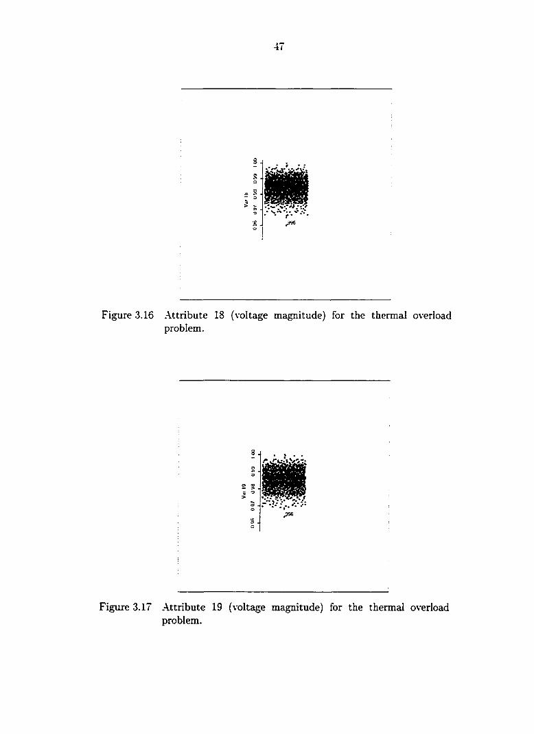
47

Figure 3.16 Attribute 18 (voltage magnitude) for the thermal overload problem.

Figure 3.17 Attribute 19 (voltage magnitude) for the thermal overload problem.

48

var?

Figure 3.18 Attribute 17 (line flow) versus subarea load for the thermal overload problem.

Var2

Figure 3.19 Voltage magnitude 7 versus subarea load for the thermal over­load problem.

49

I I ' I 0.7 OB 0 0 to Vdr2

Figure 3.20 Voltage magnitude 9 versus subarea load for the thermal over­load problem.

. i.;.. :.(•%> •

Figure 3.21 Generation A versus subarea load for the thermal overload problem.

00

! ^ /

• t I •

t • *V • •• ••

° "er/, oac/ P o6/,

Figure 3.24 A view of data for the thermal overload problem with the orig­inal data set.

. iy- • ^

'9..

» • •• *. * • V *1" -N • " • * • • • •

1

Figure 3.25 A view of data for the thermal overload problem with the orig­inal data set.

Figure 3.26 A view of data for the thermal overload problem with the al­tered data set.

Figure 3.27 A view of data for the thermal overload problem with the al­tered data set.

Figure 3.28 A \"iew of data for the thermal overload problem with the al­tered data set.

Figiire 3.29 A view of data for the voltage instability problem.

54

4 FEATURE SELECTION

4.1 Introduction

Security assessment studies have traditionally depended on engineering judgment to

select the critical parameters, i.e.. to select the parameters to be used in characterizing

the boundar\' for each security problem. The goal of this chapter is to develop an au­

tomatic approach to select critical parameters from the critical parameter candidates.

More specifically, the goal is to select the best critical parameters for the entire op­

erating range, not necessarily for any one particular operating point. Once candidate

critical parameters have been selected and a database has been generated, this becomes

a standard feature selection problem. It is not intended that automatic feature selection

will replace the engineering judgment, but rather it is intended that it will enrich the

judgment by confirming and extending physical understanding.

Feature selection is a process to identify a subset of the initial attributes, which

are also called features or parameters. The words attribute, feature, and parameter

will be used interchangeably in this dissertation. It can be thought of as a search

problem over the space of all combinations of features where a function is used to evaluate

what is "best". Also, it may be possible to combine and mathematically transform the

original attributes so that one can obtain new attributes that condense the maximum

discriminatorv- information from the available data. This is so called feature extraction.

In this dissertation, no distinction between these two cases, feature selection and feature

extraction, is treated: both are called feature selection.

55

Following a brief literature overview in the next section three classes of feature

selection methods are discussed: cluster analysis, Kohonen self-organizing map, and

genetic algorithm based methods.

4.2 Literature overview

As indicated in reference [61], researchers in the statistics and pattern recognition

communities have investigated feature subset selection problems for decades [51. 52. 53,

54. 55, 56], but most work has concentrated on subset selection using linear regression,

which is not verv- effective for highly non-linear problems. However, some statistical

methods, such as principal component analysis, are still useful for analyzing some rela­

tionships among features. Zayan et al. [63] have compared the minimum entropy method

and the Karhunen — Loeve expansion method for dynamic security classification and

concluded that the former is better. Muknahallipatna et al. [64] have compared the

linear correlation method and discriminant analysis and found that the latter is better.

In the machine learning literature, the most closely related work is MLC++ software^

and Predict software [57]. MLC+-1- uses a statistical method to search solution space.

The Predict software, in a way similar to [58], uses the genetic algorithm to search the

solution space. Downey et al. [59] also use the genetic algorithm to search the solution

space but use a statistical method to do the evaluation.

The selection of attributes is based only on the ability to predict the output. There

is no efficient way to account for cardinality constraints on the feature set although there

are several techniques that have attempted to find minimimi feature subsets (see [62]

for a discussion). Furthermore, there is no capability to preselect some features into the

solution. Therefore, a genetic algorithm based neural network feature selection tool was

developed in [61] and refined in this dissertation.

'This machine learning software was developed by Stanford University and is a\-ailable in the public domain.

56

4.3 Critical parameter candidates for the sample system

In the sample as introduced in Chapter 1. there are 32 critical parameter candidates

for the thermal overload problem and 37 critical parameter candidates for the voltage

instability problem. They are listed in Table 4.1. The objective of feature selection is

to select critical parameters from these candidates.

Table 4.1 Critical parameter candidates for the thermal overload and volt­age instability problems

.Attribute Thermal Voltage .Attribute Thermal Voltage number overload instability number overload instability 1 Gen.\ Gen.A. 20 Volt3 Volt3 2 Load Load 21 Vblt4 Volt4 3 Gen2 Gen2 22 Volt5 VoltS 4 Gen3 Gen3 23 V'olt6 Volt6 5 Flowl Flowl 24 Volt 7 Volt7 6 Flow2 Flow2 25 Volts Volt8 7 FIow3 Flow3 26 Volt9 Volt9 8 Flow4 Flow4 27 Volt 10 Volt 10 9 Flow5 Flow5 28 Volt 11 Volt 11 10 Flow6 Flow6 29 Volt 12 Volt 12 11 FIow7 Flow7 30 Volt 13 Volt 13 12 Flow8 Flow8 31 Volt 14 Volt 14 13 Flow9 Flow9 32 Flow 14 Flow 14 14 Flow 10 Flow 10 33 Qma.xl 15 Flow 11 Flow 11 34 Qmax2 16 Flow 12 Flow 12 35 Qmax3 17 Flow 13 Flow 13 36 Qmax4 18 Vbltl Voltl 37 Qmax5 19 Volt2 Volt2

4.4 Statistical method - Cluster analysis

Cluster analysis [73] can be used to anedyze similarities or dissimilarities among

groups of objects, i.e., patterns (Q-analysis) or attributes (R-analysis). There are many

cluster analysis methods in statistics. Hierarchical cluster analysis is one which results

in a tree or dendrogram showing the hierarchy of similarities among all pairs of objects.

According to [73, p.21], hierarchical cluster anal\*sis is more widely used than nonhier-

01

archical cluster analysis such as the k-means clustering method because of its simplicity

in mathematics and its effectiveness in practice. The general procedure for hierarchical

cluster analysis is as follows:

• Form a data matrix: The columns represent attributes and the rows represent

patterns.

• Normalize the data matrix: Normalize the data so that attributes contribute more

equally to the similarity calculation. For example, if the range of values on the first

attribute is much greater than the range of \-alues of the second, the first attribute

will cany more weight in determining the similarities among objects.

• Compute similarities between pairs of objects: Use a distance measure (e.g., Eu­

clidean) to compute similarities between pairs.

• Execute a clustering method to produce a tree or dendrogram: Show the hierarchy

of similarities between peiirs of patterns or attributes using a tree or dendrogram.

This is especially applicable to attribute similarity analysis or when the number of

patterns is not large so that one can clearly plot the clustering tree.

The hierarchical cluster analysis has been applied to the data set for the thermal

overload and voltage instability problems. The clustering tree for the thermal overload

problem is shown in Figure 4.1. One can see that the attributes form several clusters ac­

cording to their similarities. The result is reasonable in terms of physical interpretations

of these attributes. For example, attributes 9 (Flow5) and 17 (FlowlS), 10 (Flow6) and

11 (Flow?) are flows of circuits in series, respectively, and attributes 16 (Flowr2) and

32 (Flowl4) are flows of a transformer and a line in series. As to attributes 13 (FIow9)

and 14 (FlowlO), they are effectively in parallel from inspection of the one-line diagram

and obser\-ation of power flow variations. The plot shows that the two attributes in each

58

I

n i

n n n WCMCM^CMcviCM'-'-WCMCVJCViCVi

Figure 4.1 Cluster tree for the data set of the thermal overload problem

pair are located closely in the tree. Attributes 18 (Voltl) to 31 (Voltl4) are all of the

bus voltages located in the same region of the system.

Figure 4.2 shows the clustering tree for the voltage instability problem. One can also

observe the similar phenomena. For example, attributes 9 (Flow5) and 17 (Flowl.3). 10

(Flow6) and 11 (Flow?) are flows of circuits in series, respectively.

For feature selection, a straightforvvard method based on cluster analysis is to pick up

one attribute from each major cluster, which includes more attributes than other clusters.

For the thermal overload problem with cardiuedity level 8, for example, attributes 5

(Flowl), 9 (Flow5), 10 (Flow6), and 18 (Voltl) can be selected attributes in addition

to preselected attributes 1 to 4. However, the cardinality level should be specified in

ad^vance.

59

CM ^

O CVJ

CO CO

nTfTrnnTn- -n II I ^ o>r^

CO CO CO

CM

n

coca CO

ocoo)ocoo)sr:ip«c3^co'^ OJCMCMCOf-^WcNJCNJ ^^CMCMW

Figure 4.2 Cluster tree for the data set of the voltage instability problem

4.5 Neural network method - Kohonen self-organizing map

As discussed in Chapter 3. the Kohonen self-organizing map attempts to represent

a data set by a smaller one, by reducing either the number of input patterns or the

number of attributes while topologically preserving similarities present in the input

vectors. When it is used to reduce the number of attributes, it can be \ie\ved as a

feature selection tool.

Figures 4.3 and 4.4 are organized maps for the thermal overload and voltage insta­

bility problems. The number in a circle represents the number of attributes clustered.

Table 4.2 lists each node with the associated attributes. From the maps and the table,

it can be seen that the results are quite similar to those from cluster analysis. For in­

stance, attributes 18 through 31 for the thermal overload problem are clustered because

they are all bus voltage magnitudes. Features 9 and 17 are clustered for both thermal

overload and voltage instability problems.

For feature selection, a straightforward method based on Kohonen self-organizing

60

Figure 4.3 A 4x4 organized map of attributes for the thermal overload problem.

Figure 4.4 A 4x4 organized map of attributes for the voltage instability problem.

61

Table 4.2 Nodes on the map with their associated attributes for the thermal overload problem.

Node Features (Thermal overload) Features (Voltage instability) 1 18-31 (Voltl-Voltl4) 18-21 (Voltl-Volt4), 25 (Volt8). 26 (VoltQ),

28-30 (Voltll-Voltl3). 34 (Qma.x2) 2 22-24 (Volts-Volt7), 27 (VoltlO). 31 (Voltl4) 3 9 (Flow5). 17 (Flowl3) 4 8 (Flowl2) 13 (Flow9). 14 (FlowlO). 33 (Qma.xl) 5 6 16 (Flowl2) 2(Load) 4 10 (FIow6). 32 (Flowl4) 4 (Gen3), 35 (Qmax3) 8 6 (Flow2), 11 (Flow?) 1 (Genl) 9 2(Load) 9 (Flow5). 16 (Flowr2). 17 (Flowl3) 10 11 36 (Qmax4). 37 (Qmax5) 12 5 (Flowl), 7 (Flow3). 12 (Flow8) 13 1 (Genl). 13 (Flow9), 14 (FlowlO) 8 (Flow4), 10 (Flow6). 32 (Flowl4) 14 5 (Flowl). 6 (Flow2). 11 (Flow7). 12 (FlowS) 15 3 (Gen2). 4 (Gen3) 16 15 (Flowll) 3 (Gen2). 7 (Flow3). 15 (Flowll)

map is to pick up one attribute from each major node, which includes more attributes

than other nodes. For the thermal overload problem with cardinality level 8, for example,

attributes 5 (Flowl), 9 (Flow5), 10 (Flow6), and 18 (Voltl) can be selected attributes

in addition to preselected attributes 1 to 4. However, the cardinality level should be

specified in advance.

4.6 Genetic algorithm method

The genetic algorithm (GA) [65, 66] is used to search the feature space. The e\-alua-

tion function is the fitness function which includes network accuracy, feature cardinality,

and feature constraints such as set controllability. Figure 4.5 illustrates the basic func­

tional structure of the developed genetic algorithm based neural network feature selection

tool (GANN), which was initially designed and implemented by Mr. Qianglin Zhao [61].

62

4.6.1 Design of GANN

Figure 4.5 shows the functional structure of GAXX. Since the two important com­

ponents are the search approach and the evaluation function, they are discussed first,

and then the procedure in Figure 4.5 is explained.

f 'npui I data set j

INITIALIZATION

Select mitioJ

population

of solutions

FITNESS

CALCULATIONS

Use neural network (c compute tltness of population

members

Cntical ponmet

EVOLUTION

Improve the population

via crossover

and mutation

Figure 4.5 Bcisic functional structure of GAXX

4.6.1.1 Search Approach

If there are n candidate features, the solution space will consist of 2" possible so­

lutions. Even if the number of candidate features can be reduced to 30 or 40 using

engineering judgment, the solution space is still verv* large (2^° = 1.1 x 10^) so that

exhaustive search is not practical. Genetic algorithms are ver\' effective in solving com­

binatorial problems for which a performance measure, i.e., a fitness function, can be

defined for each combination under consideration. Therefore, the GA is used for an

efficient search for the best subset of features. In this design, the user specifies pa­

rameters that should be forced into the solution to satisfy the feature controllability

constraint. The user also specifies a cardinality range. The GA then identifies the most

accurate solution containing the forced parameters for each cardinality level in the spec-

63

ified range. Finally, the user can easily select the solution that offers the best tradeoff

between accuracy and cardinality.

4.6.1.2 Evaluation function

The evaluation function is used in fitness calculations, as shown in Figure 4.5. to

calculate the fitness for a possible solution. The larger the fitness, the better the feature

subset. The fitness of the i-th individual in the population can be computed according

to Fi = ujiFii + woF-ii where Fu and Foi are the fitness components corresponding to

the neural network accuracy and cardinality, respectively, and wi and ito are their corre­

sponding weights. Fii is taken £is the reciprocal of the average absolute error computed

by testing a neural network trained with inputs corresponding to the selected attributes

of the individual. Fo, is equal to Uj, the cardinality level of individual j. if Uj is smaller

than the desired cardinality level: otherwise, it is zero. Weights wi and wo are set to 1.0

and 3000.0, respectively. The cardinality component is weighted much higher than the

accuracy component and therefore dominates the early generations during evolution so

that members in later generations are those with the desired cardinality, and evolution

proceeds to maximize accuracy.

4.6.1.3 Procedure of GANN

The procedure of GANX includes the following steps:

1. Population initialization - Randomly generate the initial population consisting of

M members. Each member is a possible solution represented as a binar\- vector

whose length is equal to the number of candidate features. A "1" means the feature

is selected and a "0" means the feature is not selected.

2. Fitness calculation - Calculate the fitness \-alue of each member in the current

population.

64

3. Elitist strategy - Select the first N members with the largest fitness values to be

directly placed into the next generation.

4. Crossover - Select M — N members using roulette wheel selection to be placed

into a mating pool. With probability proportional to fitness values, pick a pair

of parents and perform crossover operation with a high probability to generate

offspring.

5. Mutation - Perform mutation operation with a low probability on the offspring to

obtain a new generation of population.

6. Stopping criterion check - Check the stopping criterion: if it is satisfied, stop:

other\vise, go to step 2. A limit on the number of generations as the stopping

criterion. E.xperience with the algorithm has resulted in a choice of 200 for this

limit.

4.6.1.4 Neural network

The multilayer perceptrons (MLPs) w-ith backpropagation (BP) learning algorithm is

used to perform the evaluation for different feature sets. In order to limit computational

time, we use a one hidden layer neural network with only one neuron in the hidden

layer, .\fter selection of the best features using a simple fixed neural network, we apply

£in optimization procedure to select and train the best neural network architecture, in

terms of the number of hidden neurons, using a fixed feature set.

4.6.2 Application to the sample system

For the line thermal overload problem, we ran GANN for 11 different cardinality

levels, from 5 to 10, with parameters 1-4 forced into the solution. The results are given

in Table 4.3. The result of cardinality level 8 is chosen because it provides the best

65

Table 4.3 Feature selection results for the line thermal overload with cardi­nality levels 5-10 (using MLPs)

Parameter Cardina ity Level Name 5 6 1 8 9 10 Genl 1 1 1 1 1 1 Load 1 1 1 1 1 1 Gen2 1 1 1 1 1 1 Gen3 1 1 1 1 1 1 Flowl 0 0 0 0 0 0 Flow2 0 0 0 0 0 0 Flow3 0 0 0 0 0 0 Flow4 0 0 0 0 0 0 Flowo 0 1 0 0 1 1 Flow6 0 0 0 0 1 0 Flow? 0 0 0 0 0 0 FlowS 0 0 0 0 0 0 Flow9 0 0 0 0 0 0 Flow 10 0 0 0 0 0 0 Flowl 1 0 1 0 0 0 0 Flow 12 0 0 0 0 0 0 Flow 13 1 0 1 1 0 1 V'oltl 0 0 0 0 0 1 Volt2 0 0 0 0 0 0 \blt3 0 0 0 0 0 0 V"olt4 0 0 1 1 1 0 VoIt5 0 0 0 0 0 0 Volte 0 0 0 0 0 0 V'oltT 0 0 0 0 0 0 Volts 0 0 0 0 0 0 Volt9 0 0 0 0 0 1 Volt 10 0 0 0 0 0 0 Voltll 0 0 0 0 1 0 Volt 12 0 0 0 1 0 1 Voltl3 0 0 0 0 0 0 Volt 14 0 0 0 0 0 0 Flow 14 0 0 1 1 1 1 Average Error 0.0315 0.0207 0.0090 0.0082 0.0084 0.0078

66

tradeoff between cardinality and error. The average error is given as a percentage of 600

A. which is the maximum flow on the overloaded line. The results generally agree with

engineering judgment. For example, parameters Flow5, FlowlS, and Flowl4 are selected

the most often since these parameters represent the flows on the overloaded circuit

FlowlS (Flow5 and FlowlS are approximately in series) and the outaged circuit (Flowl4).

The other parameters selected for cardinality level 8 are bus voltage magnitudes near

the overloaded or outaged circuit.

For the voltage instability problem, we ran GANX for 5 different cardinality levels,

from 9 to 13. with parameters 1-4 forced into the solution. The results are given in

Table 4.4. The results also generally agree with engineering judgment. For example, pa­

rameters 33 and 36 are always selected since they represent two synchronous condensers

close to the load bus with deficient reactive power. The result of cardinality level 11 is

chosen because it provides the best tradeoff between cardinality and error. Here, the

average error is given as a percentage of 200 MVAr, which is the reactive power margin

on the the load bus with the most deficient reactive supply.

For both problems, the critical parameters include load, generations, line flows, and

bus voltage magnitudes. For the voltage instability problem, an additional tv-pe of

critical parameter is a\-ailable reactive power supply. There are three a\-ailable reactive

power supplies corresponding to three different groups of generators, Qmaxl.Qmax'l,

and QmaxZ, each of which is the sum of the reactive capacities for the committed

generators in that group. These values change accordingly as the unit commitment

status in each group changes.

It is necessary to point out that GANN is not guaranteed to give the best solution

because of its stochastic nature and the fact that the nimiber of evolutions can not be

infinite. However, given a finite and sufficiently large number of evolutions, it has been

found that GANN will always produce a good solution.

67

Table 4.4 Feature selection results for the voltage instability with cardinal­ity levels 9-13 (using MLPs)

Pcirameter Name

Cardinality Level Pcirameter Name 9 10 11 12 13 Genl 1 1 1 1 1 Load 1 1 1 1 1 Gen2 1 1 1 1 1 Gen3 1 1 1 1 1 Flowl 0 1 0 1 0 Flow2 0 0 0 1 0 Flow3 0 0 0 0 0 Flow4 0 0 0 0 0 Flow5 0 0 0 0 0 Flow6 0 0 0 0 0 Flow? 0 0 0 0 0 FlowS 0 0 0 0 0 Flow9 0 0 1 0 1 Flow 10 0 0 0 0 0 Flow 11 0 0 0 0 1 Flow 12 0 0 0 0 0 Flow 13 0 0 1 1 0 Vbltl 0 1 0 0 0 Volt2 0 0 0 0 0 VoIt3 0 0 0 0 0 Volt4 0 0 0 0 0 Volto 0 0 0 0 1 Volte 0 0 0 0 0 Volt" 1 0 1 0 1 \blt8 0 0 0 0 0 Volt9 0 0 0 0 0 VoltlO 0 0 0 0 1 Volt 11 0 0 0 0 0 Voltl2 0 0 0 0 0 Volt 13 0 0 0 0 1 Voltl4 1 1 1 1 1 Qmaxl 1 1 1 1 1 Qmax2 1 0 0 0 0 Qmax3 0 0 1 1 0 Qmax4 1 1 1 1 1 Qmaxo 0 1 0 0 0 Flow 14 0 0 0 1 0 Average Error 0.0824 0.0742 0.0665 0.0736 0.0783

68

4.6.3 Improvement on solution speed

4.6.3.1 GANN with radial basis function networks

There are some problems when the GA is used to do feature selection where a neu­

ral network architecture with standard backpropagation (BP) algorithm is adopted to

compute fitness. One of them is that the standard BP algorithm is verv' slow. Since

each potential solution requires neural network training, the training speed is the most

significant influencing factor with respect to the overall solution time. This is a ma­

jor disadvantage of using G.A. with the BP algorithm to do feature selection for neural

networks. For instance, it took 88886 seconds of CPU time to obtain the solution for

cardinality 8. To overcome this problem mentioned above, the BP algorithm in G.A.XX

is replaced by a radial beisis function network with a fast training method.

If we view the neural network design problem as a curve fitting problem in a high-

dimensional space, learning is equivalent to finding a surface in a multidimensional space

that best fits the training data. Generalization is then equivalent to using this multi­

dimensional surface to interpolate the test data. Such a viewpoint is indeed the moti­

vation behind the method of radial basis functions (RBFs). Broomhead and Lowe [67]

first explored the use of FlBFs in neural networks. Moody and Darken [68], Renals and

Rohwer [69], and Poggio and Girosi [70] among others made major contributions to the

theor>', design, and application of RBF networks.

The basic architecture of a RBF network is shown in Figure 4.6. It includes three

entirely different layers. The first layer is an input layer for which each node corresponds

to an attribute of an input pattern. The second layer is a hidden layer that is used to

cover the whole input space with each node covering a different region. The third layer

is an output layer responding to the input patterns. The transformation from the input

layer to the hidden layer is nonlinear, whereas the transformation from the hidden layer

to the output layer is linear. As illustrated in Figure 4.7, an activation function for a

69

«P(.)

0

y

Figure 4.6 A radial basis function network

iiidden layer node is a locally radially symmetric function (typically Gaussian function),

where the output decays to zero as the distance (usually Euclidean distance) between

the input vector and its center increases, see Figure 4.7.

There are two important parameters, center and width, associated with an activation

function. center is a vector with the same dimension as the input pattern, which

represents a cluster center of the input space. .A. width is used to control the spread

of the RBF so that its output decays more slowly or more rapidly as the distance

between the input vector zmd the center increases. Each RBF responds to a small

convex region of the feature space. .A. large number of these functions cover the entire

Output

0

Distance to centcr ^

Figure 4.7 A radial basis function in one-dimensional space

70

feature space so that the output layer neurons can join them with different weights to

accomplish the function approximation or classification. Figure 4.8 shows a portion of

two-dimensional feature space covered by RBFs.

Without loss of generality, consider a RBF network with only one output. The output

of such a network can be expressed as

X,

Figure 4.8 A portion of two-dimensional feature space covered by RBFs

/(x) = i^u.-iV^.(||x-c,|i) (4.1) 1=1

where x is an input pattern. Cj is the center for hidden node i. ivi is the weight between

hidden node i and the output node, and wq is a bias weight. M is the number of hidden

nodes, is the acti\-ation function for the hidden layer. The norm ||-|| can be Euclidian

or Mahalanobis distance [75. p. 87]. A RBF approximation using Gaussian functions is

considered below.

WTien y(-) is a Gaussian function, (4.1) can be seen as approximating a probability

density by a mixture of Gaussian functions. The Gaussian function can be expressed as

ip{u) =6 2^

The output can then be expressed as

(4.2)

71

M /(x) = Wie (4.3)

:=1

RBF networks provide an attractive approach for function appro.\imation because of

their flexible structure, fast training, powerful generalization capability, and conceptual

elegance. Park and Sandberg [71] have shown that RBF networks with Gaussian basis

functions are universal function approximators. Girosi and Poggio [72] have shown

pointwise convergence property of a class of RBF networks.

There are different training strategies for RBF networks [77]. Since the linear weights

associated with the output node tend to evolve more slowly than the nonlinear activation

functions of the hidden nodes, it is reasonable to train the network layer by layer to get

fast training speed. The training strategies can be divided into the following three classes

depending on how the centers of the RBFs are specified.

Fixed centers selected randomly

The simplest and fastest approach is to randomly select centers from the training

data set and keep them constant throughout the training. This is reasonable provided

that the training data are well representative of the problem. The widths for all RBFs

are also fixed and are the same. This width can be taken as the standard de%-iation of

the Gaussian function, expressed as

d G — (4.4)

sfWl '

where d is the maximum distance between the selected centers. Such a choice for the

standard deviation a is to ensure that RBFs are neither too peaked to cover the whole

input space nor too flat to distinguish between dissimilar input patterns.

Then, the only parameters that need to be trained are the weights between the hidden

and output layer, which can be computed directly by solving linear equations. Usually

the number of training patterns is much larger than the number of selected centers.

72

so the resulting linear equations are overdetermined. A straightforward procedure for

solving such equations is to use the pseudoinverse method [67] to obtain a solution with

the minimum least square error.

The linear weights can also be solved by iteration using a gradient-descent technique.

This approach is much faster than the BP algorithm for MLPs because it adjusts only

the weights between the hidden and output layer whereas MLPs adjust weights between

all layers. The generalization capability and accuracy level depends on the number of

centers and the representativeness of the training data set to the problem that is being

studied.

Unsupervised selection of centers

In principle, any unsupervised or clustering algorithm can be used to specify the

centers. For example, one may use k-means clustering algorithm [68]. hierarchical cluster

analysis, or self-organizing map. After determining the centers, one may obtain the linear

weights either by directly solving the linear equations or by iteration.

Supervised selection of centers

This is the most flexible but most time-consuming training approach among the three

strategies. The centers, widths, and linear weights are all adjusted through a supervised

training process. A natural candidate for such a process is an error correction iteration

algorithm using gradient-descent technique.

The squared error for the output can be written as

- k=i

The update equations for the linear weights, centers, and widths are given as fol­

lows [77, Chapter 7]

E (4.5)

73

Wi{t + 1) = w,{t) + r/i - yk)e (4.6)

c,_,(f+l) = c^Jit) + ^2^[ak-yk)u:^[l)e -• • {xkj - c^J{t)) (4.7)

a^{t + 1) = af{t) + r/3 - yk)u;,:^k • (4.8)

For the thermal overload problem. GAXX was run with RBFXs using the learning

algorithm of fixed centers, for 5 different cardinality levels, from 5 to 10. with parameters

1-4 forced (preselected) into the solution, meaning that all solutions provided by G.A.XX

will have GenA, AreaLoad, GenB, and GenC. in addition to some other parameters.

The results of GAXX runs are given in Table 4.5 [82]. The level 8 cardinality is

chosen because it represents the best tradeoff between cardinality and accuracy.

The results generally agree with engineering judgment. For example. Flow5 and

V'oltl are chosen most often; FIow5 represents the flow on the overloaded circuit and

Voltl is a bus voltage close to the outaged circuit. The results show that GAXX with

RBFXs using the learning algorithm of fixed centers runs faster than with MLPs using

the BP learning algorithm. For example, at cardinality level of 8, it took almost 10 times

faster for the former than the latter (8903 seconds \vith RBFXs versus 88886 seconds

with MLPs).

For evaluation of the feature selection effect, the test results with 8 selected attributes

and with all 32 attributes are shown in Figure 4.9. It can be seen that the test error

is much smaller using the selected attributes. Furthermore, training with fewer selected

attributes takes less time than with ail 32 attributes although the CPU time is increasing

w-ith the nimiber of centers in both cases, as shown in Figure 4.10. It is noted that the

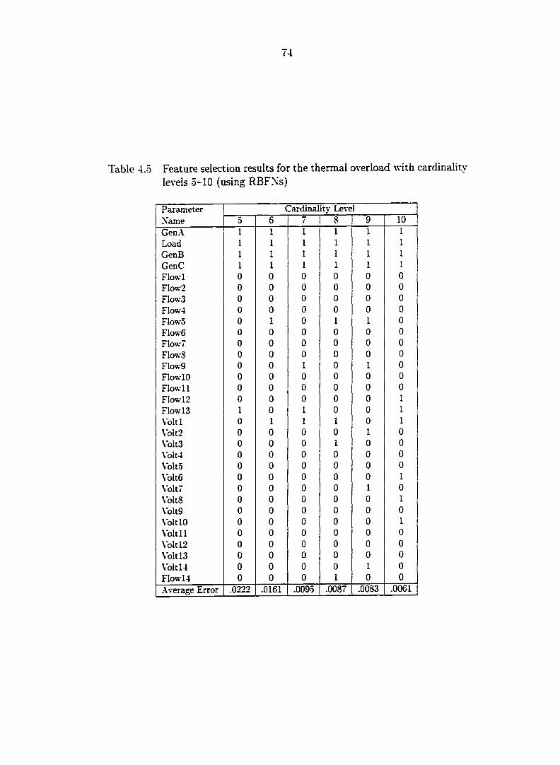
74

Table 4.5 Feature selection results for the thermal overload with cardinality levels 5-10 (using RBFXs)

Parameter Name

Cardinality Level Parameter Name o 6 7 8 9 10 GenA 1 1 1 1 1 1 Load 1 1 1 1 1 1 GenB 1 1 1 1 1 1 GenC 1 1 1 1 1 1 Flowl 0 0 0 0 0 0 Flow2 0 0 0 0 0 0 Flow3 0 0 0 0 0 0 Flow4 0 0 0 0 0 0 Flow5 0 1 0 1 1 0 Flow6 0 0 0 0 0 0 Flow? 0 0 0 0 0 0 Flows 0 0 0 0 0 0 FIow9 0 0 1 0 1 0 FlowlO 0 0 0 0 0 0 Flow 11 0 0 0 0 0 0 Flowl2 0 0 0 0 0 1 Flow 13 1 0 1 0 0 1 Voltl 0 1 1 1 0 1 Volt2 0 0 0 0 1 0 Volts 0 0 0 1 0 0 \blt4 0 0 0 0 0 0 Volt 5 0 0 0 0 0 0 \blt6 0 0 0 0 0 1 Volt? 0 0 0 0 1 0 VoItS 0 0 0 0 0 1 \blt9 0 0 0 0 0 0 Volt 10 0 0 0 0 0 1 Voltll 0 0 0 0 0 0 Volt 12 0 0 0 0 0 0 Volt 13 0 0 0 0 0 0 Voltl4 0 0 0 0 1 0 Flowl4 0 0 0 1 0 0 Average Error .0222 .0161 .0095 .0087 .0083 .0061

^ 0

0.0251

- - Befora feature selection

After feature selection

0.02

0015

S 0.01

0005

100 Number of centers

Figure 4.9 Test errors versus number of centers (random selection of cen­ters)

250

Before feature selection After teature selection

200

§ 150

100

20 40 50 80 100 NumOer of centers

Figure 4.10 CPU time versus number of centers (random selection of cen­ters)

76

accuracy level is improved with the increase of the number of centers, but this is

achieved at the price of solution speed decrease. Therefore, the user must make a

tradeoff between accuracy and speed by choosing the number of centers. Like choosing

the hidden nember of hidden nodes for MLPs, unfortunately, there is no theoretical

guidance for choosing the number of centers for RBFXs.

4.6.3.2 Genetic algorithm with k-nearest neighbor method

To further improve the solution speed, the k-nearest neighbor method instead of

neural networks is used to evaluate feature sets. Table 4.6 shows the feature selection

results using RBFXs and KXXs for the thermal overload problem. From the table,

we can see that the solution speed with KXXs is much faster. However, the error will

be much larger if we use KXXs to predict the postcontingency performance measure

based on the selected features. Xote that MLPs are still to be used in postcontingency

performance measure prediction.

Table 4.6 Comparison of feature selection results using RBFXs and KXXs for the thermal overload problem

Radial basis function networks k-nearest neighbors Features selected 1.2.3.4.9.17.18.32 1.2.3.4.9.17.19.32 Running time 8903 4709 .Average error 0.0012 0.0270

4.7 Comparisons of different feature selection methods

The feature selection methods discussed above include the cluster analysis, the Ko-

honen self-organizing map, cind the genetic algorithm based methods. The genetic algo­

rithm based methods include those with MLPs, RBFXs, and KXXs. Two comparisons

will be made as follows.

I i

4.7.1 Solution speed

According to the decreasing order of solution speed, the first is the cluster analysis

followed by the Kohonen self-organizing map. and the genetic algorithm based methods

are the last. Of the \^riations of the genetic algorithm based methods, the method with

KXXs is the fastest, that with RBFNs is the second fasted, and that with MLPs is the

slowest. Table 4.7 lists the solution time for the genetic algorithm based methods with

MLPs. RBFNs, and KXXs with cardinality level 8 for the thermal overload problem.

Table 4.7 Comparison of solution time (s)

.MLPs RBFNs K.XNs S8886 8903 4709

4.7.2 Prediction accuracy

The MLPs are used to predict the postcontingency performance measure using se­

lected features because they are the most accurate. To compare the accuracy levels for

features selected by different methods, a MLP with one hidden neuron is trained and

tested using these features. Table 4.8 lists the selected features and the average errors

for the genetic algorithm based methods with MLPs, RBFXs. and KXXs with cardinal­

ity level 8 for the thermal overload problem. From this table, we can find the following

facts. First, the accuracy levels for cluster analysis and Kohonen self-organizing map

\-ary depending on what features are selected from the clusters or nodes. Second, the

accuracy level for GAXX with MLPs is highest. This is reasonable because the features

selected by GANX with MLPs were used to train a MLP itself. The accuracy level for

GAXX with RBFXs is lower than that for GAXX with MLPs but higher than that for

GAXX with KXXs. For more thorough comparison, it is better to consider the variances

as well.

78

Table 4.8 Comparison of prediction accuracy

Method Features Selected .\verage Error G.\XN--MLP 1.2.3,4.17.21,29.32 0.0029 G.A..\N-RBFN 1,2,3.4,9.17,18.32 0.0034 GANN-KNN 1.2.3,4.9,17,19.32 0.0036 Cluster .Analysis 1.2.3.4.5.9.10.18 0.0051

1,2.3,4.11.12.17.18 0.0045 1.2.3,4.9,12.18.32 0.0035 1.2.3.4,9,12,15.18 0.0032 1.2.3.4,10,13.16,17 0.0045

Kohonen .Map 1.2.3.4.5.9.10.18 0.0051 1.2.3.4.5.6.9,18 0.0041 1.2.3.4.7.17.18.32 0.0032 1.2.3.4.7,17.20.32 0.0037 1.2.3.4.12.17.18.32 0.0032

4.8 Summary

Three classes of feature selection methods have been discussed: cluster analysis.

Kohonen self-organizing map, and genetic algorithm based methods. Cluster analysis

and Kohonen self-organizing map divide the features into various clusters according to

their similarities. They are fast. Then, for feature selection, only one feature needs to

be picked up from each cluster to represent this cluster. Therefore, there are different

feature selection results depending on which feature is selected from each cluster. Some

results may give higher accuracy, some results may give lower accuracy. There is no

guarantee that a good accuracy is achieved.

In consideration of this fact, genetic algorithm based methods are preferred. Among

GAXX with MLPs, GAXX with RBFXs, and GAXX with KXXs. GAXX with KXXs has

fastest solution speed but lowest accuracy, and GAXX with MLPs highest accuracy but

slowest solution speed, which should be used? By making a trade-off between solution

speed and accuracy, GAXX with RBFXs is recommended because it is much faster than

GAXX with MLPs without much loss of accuracy.

79

5 TRAINING AND USING NEURAL NETWORKS FOR

BOUNDARY APPROXIMATION

5.1 Introduction

After generating data and selecting features, the next step is to train neural networks

using the data and features to predict postcontingency performance given precontingency

information, for a single contingency. Issues in training and using neural networks are

discussed in this chapter. Overfitting. underfitting, and accuracy improvement near the

boundar\- during training are addressed first to achieve the expected accuracy. Then,

confidence interval calculation formulas for neural network outputs are derived and im­

plemented for MLPs. Finally, sensitivities of neural network outputs with respect to

inputs are derived and implemented for MLPs.

5.2 Training neural networks

5.2.1 Overfitting and underfitting

Overfitting and underfitting are ver\* important problems for neural network training.

If the number of degrees of freedom of the neural network is too high (low) with respect

to the training set, the neural network is verv- likely overfitted (underfitted). If the neural

network is underfitted, it is difficult to reach an acceptable convergent training error. If

the neural network is overfitted, the training error may be low but the test error can be

much higher. A neural network is said to memorize rather than learn the training data

80

if it responds to a sample in the training data set in the same manner as it was trained,

but it responds to other samples with ver\' poor results. In the case of overfitting. a

neural network just memorizes the training data, hence the generalization capability is

ver\- poor. To alleviate this problem, the following approaches may be used:

Underfitting detection by a trial and error approach

After the training process has converged, if the training error is higher than the

\'alue one would e.xpect, it means that an underfitting occurs. Therefore, the network

complexity, i.e.. the number of degrees of freedom of the neural network, should be

increased and a new network trained. In the case of MLPs with one hidden layer,

the number of hidden neurons should be increased. If an underfitting still occurs after

training the new network, another trial is needed with respecc to a more complex network

structure.

Overfitting detection by monitoring and comparing training error and test error

Initially, both training error and test error decrecise with training iterations, then

flatten out until some point where the training error still decreases but the test error

begins to increcise. This point is where overfitting occurs. Figure 5.1 illustrates this

situation. However, it is not always apparent to see this point because some oscillations

of test error may occur.

5.2.2 Exploration of improvement on accuracy near the boimdary

Because the ultimate goal of this research is to produce boundaries, which are con­

tours of constant sv'stem performance, the accuracy of the function approximation

R = /(X)

81

Test

Training

Number of iterations

Figure 5.1 Variation of training and test errors with the number of itera­tions.

at the boundar\- R = Rq is a major concern. However, because no other x-alues of R are

ultimately revealed to the operator, it is much less concerned with the accuracy of

at points not on the boundar\\ Therefore, the accuracy off the boundar>" can be sacrificed

if the accuracy on the boundarv- can be simultaneously improved. One method has been

identified to do this. This method is called weighted output errors.

During training, let the output error near the boundary* have larger weight than that

far away from the boundary in the total error of all the outputs. The following function

is used to obtain a weight w for the desired output d where x > 1 (the smaller x. the

larger the weights for points close to the boundarj-) and d = 0 occurs for a point on the

boundary-. Figure 5.2 shows a plot of fxmction (5.1) for x = 8. It Ccin be seen that the

farther the desired output is from the boundary-, the smaller the weight is. Figure 5.3

shows the distribution of 411 test samples. Figure 5.4 shows the test error distribution for

test samples using the weighted errors training and that using regular training. However,

R = /(X)

w = 1 — (5.1)

82

the result with weighted errors is not better than that without weighted errors for points

close to the boundar\- as it was expected. The reason may be that the weight update

approach is still the gradient descent technique, which is used for updating weights. To

find the exact explanation, it requires further investigation, which is beyond the scope

of this dissertation.

0,91

0.7

0.6

0.4

0.3

02

0.3 0.2 0.4 0.6 0.9 O.S Oesired output

0.7

Figure 5.2 Plot of function w = I — d^.

5.3 Confidence intervals for neural network outputs

WTien a trciined neural network is used for prediction, it is desirable to e\"aluate the

reliability of the performance. One way to do this is to give a confidence measure for

the neural network output.

From the view of statistics, function approximation by neural networks can be

thought of as a nonparametric nonlinear regression problem. Therefore, confidence in­

terval estimation methods for nonparametric nonlinear regression can also be used for

evaluating confidence intervals for neural network outputs. In what follows, the con-

83

0.4

0.2

•5-0.2

-0.4

-0.6

-0.8 100 150 200 250 300 350 400 450

Sample number

Figure 5.3 R \-alues for the test samples.

0.025 r

X Without weighted errors o With weighted errors

0.02 -

0.015

0.01

0.005

0.2 0.3 0.4 0.5 0.6 Distance from the boundary

Figure 5.4 Test error distributions.

84

fidence interval expressions for MLPs will be derived based on a general formula for

nonparametric nonlinear regression.

Consider a general nonlinear regression model [76] with p parameters to be estimated

and n observations

Ui = /(x,,0)+ i = (5.2)

where ij is the actual output, x is the input vector. 0 is a vector of the parameters to be

estimated, and cj is the error associated with the function /. We assume that 5,'s are

normal and independent with zero mean and common variance a-. Let 9 be the least

squares estimator of 6, then

5(«) = Zb-Zfe-S)!' (5.3) t = l

is minimized. The nonlinear function in (5.2) can be expanded in a Taylor series around

the estimated vector 9 retaining only the first order terms. Thus

/(x.,0) % f { - x . i , d )+z l {9 -9 ) . i= l r - - , n (5.4)

where

= d f { ^ , 9 ) d f { x , , 9 ) d f { x i . 9 )

d9i ' 892 ' ' d9p (5.5)

8=a

Equation (5.4) is a linear approximation of the nonlineiir fimction in (5.2) in the neigh­

borhood of 9. and it can be written as

y i - f { x i , 9 ) = ^ {9 -9 )+£ i , i = (5.6)

85

Because of the statistical independence between Q and c ^'s. given x q , the variance of

the output j/o can be expressed as

var(yo - yo) = i-ar(co) + v-ar(g^(^ - )) (5.7)

For an error Sq with a normal distribution with a mean of zero and a variance of

<7-(.V(0. cr-I„)), the distribution o i 6 — 6 can be approximated to have

.Vp(0, <7-[G^G]~^), where G is the Jacobian matrix defined as

the distribution

G =

a/(xi ,6) d0i

d f {x2 .0 ) dSi

9 f i x i .B ) ee-z

d f {x -2 .B ) dOz

d f i x i .B ) ddp

Of (x2 .8 ) aOp (5.8)

Thus, we can obtain

d f {x„ .0 ) aoi

d f iXn .B) 002

Of (Xn .9 ) dOp 6=6

var[y 0 — i/o] = = <T- + a-g^(g^g) ^go (5.9)

cr- can be approximated by

s- = '^ bt - /(Xi. 9)]-

: = i " - P

As a result, the standard error of a predicted value f{xo,6) is given by

The Student i-distribution is

yo - Vo f *'71—P ^var[?/o - j/o]

Vq - yo

(5.10)

(5.11)

(5.12)

(5.13)

86

The approximate 100(1—a)9c confidence interval on the prediction for a new observation

Xo is then given by

This is a general expression of the confidence interval for any regression problem.

The plus and minus signs in (5.14) are used to give the upper bound and lower bound of

the confidence interval. For all of the observations for which the confidence intervals are

computed, the envelopes can be obtained by connecting all of the lower bound points

and all of the upper bound points, respectively.

For the case of neural networks, weights correspond to 9 and input patterns cor­

respond to Xq. Therefore, we can easily derive the confidence interval expressions for

different types of neural networks using (5.14). The key is the calculation of deri\-atives

of the output with respect to weights [81]. which are used in formulation of G.

For MLPs with one hidden layer as shown in Figure 5.5. the derivatives of output ijj

with respect to weight Wji between the hidden and output layer can be derived as

The derivatives of output yj with respect to weight between the input and hidden

(5.14)

dVj _ ^ dv j

dwj i dv j dwj t

(5.15)

Figure 5.5 A detailed structure of a multilayer perceptron

87

layer can be derived as

dy j _ dy j dv j d z , dv j

dwik dvj dzi dt'i dwik

= iyj(^vj)wjnp^{vi)xk (5.16)

where Zi is the output of hidden node i . v j is the dot product of the outputs from the

hidden nodes and weights between the hidden nodes and output node j. >;;(•) is the

activation function of a node.

When a hyperbolic tangent function

^{x ) = a tanh(6x) gfcr _ g-6x

e'^ + '2a

— ^ ~ (5.17) 1 + e--'^ ^ '

is used as an activation function, its deri\^tive is

^ ' { x ) = ab{ l - ip ' { x ) ) (.5.18)

where a and 6 are constants specifying the range and the slope of the function, respec­

tively. Using this activation function for all of the nodes. (5.15) and (5.16) become

dy j

dwji = a6(l - y-(vj))zi (5.19)

and

= a 'b - ( l - :p-{v j ) y i v j i ( l - ~^^ iv i ) ) xk (5.20) dwik

respectively.

The confidence interval calculation method has been applied to the thermal overload

problem for a demonstration. Figure 5.6 shows the 90% confidence intervals for a portion

of test data for the thermal overload problem. It can be seen that the desired output

falls between the envelopes of the confidence interval with probability about 90%.

88

X

0.8 - X Desired output o Actual output

0.6 - — Envelope

® i) *

0.4

0.2 « / / w

- 0 .

-0.6

-0.4 i | i H • W lit

-0.8 0 5 10 IS 20 25 30

Figure 5.6 90% confidence interval for the test data of the thermal overload problem.

To apply the confidence interval calculation method to the boundar>-. simply calculate

the confidence interval and obtain the lower and upper bounds for each boundarv* point,

then connect the lower bound points and the upper bound points, respectively.

5.4 Sensitivity ansdysis of the neural network output with re­

spect to input parameters

Analyzing the sensitivity of the neural network output with respect to input parame­

ters will help operators understand the relative importance of these parameters in terms

of their contributions to av^lable security margin.

For MLPs with one hidden layer of m nodes (see Figure 5.5), the sensitivity of output

j with respect to input k can be derived as follows

89

= (5.21) 1=1

When a hyperbolic tangent function (5.17) is used for activation functions for all of

the nodes. (5.21) becomes

z;)w,k (5.22) OXk

Figure 5.7 shows the sensitivity of the MLP output with respect to the S input

parameters for the thermal overload problem. Figure 5.8 shows the sensitivity of the

MLP output with respect to the 11 input parameters for the voltage instability problem.

These sensitivity plots are with respect to a specific operating condition. For the thermal

overload problem, the most sensitive parameter is input parameter 5. which is Flowl.3.

Because the corresponding sensitivity is positive, increeising Flowl3 will make the system

more insecure. For the voltage instability problem, the most sensitive parameters are

input parameters 7 and 8, which are the two bus voltage magnitudes, \blt7 and \bltl4.

Because the corresponding sensitivities are negative, an operating condition change that

3 1 1 1 I ! ! 1 ! 1 !

2-sl-

2

1.5

1

0.5

0

-0.5

-1

-1.5 0 1 2 3 4 5 6 7 8 9 1 0

Figure 5.7 Sensitivity of the MLP output with respect to the 8 input pa­rameters for the thermal overload problem.

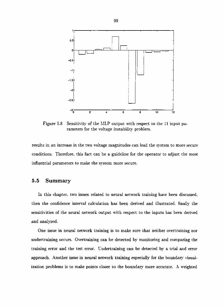
90

0.5

0

-0.5

-1

-1.5

-2

-2.5

_ 3 l ^ ^ , , 0 2 4 6 8 10 12

Figure 5.8 Sensitivity of the MLP output with respect to the 11 input pa­rameters for the voltage instability problem.

results in an increase in the two voltage magnitudes can lead the system to more secure

conditions. Therefore, this fact can be a guideline for the operator to adjust the most

influential parameters to make the system more secure.

5.5 Summsiry

In this chapter, two issues related to neural network training have been discussed,

then the confidence inter\-al calculation has been derived and illustrated, finally the

sensitivities of the neural network output with respect to the inputs has been derived

£md anzdyzed.

One issue in neural network training is to make sure that neither overtraining nor

undertraining occurs. Overtraining can be detected by monitoring and comparing the

training error and the test error. Undertraining can be detected by a trial and error

approach. Another issue in neural network training especially for the boundary- visual­

ization problems is to make points closer to the boundarv- more accurate. A weighted

- -

LJL_1

91

output error approach has been explored but is not effective.

Confidence intervals can be a measure of the neural network output reliability. The

calculation formula have been derived for the MLPs based on nonparametric nonlinear

regression. .A.n example has been given to illustrate how to calculate confidence interval

conculation for the thermal overload problem.

Sensitivities of the neural network output with respect to the inputs can provide a

control guideline for the operator to effectively adjust the system to more secure con­

ditions. The sensitivity calculation has been derived and demonstrated for the thermal

overload and voltage instability problems.

92

6 PRESENTATION TECHNIQUES

6.1 Introduction

The ultimate goal of this research is to enable highly accurate nomogram presentation

to the operator. This presentation should be fast and automatic so that it can interface

with other software and communication equipment in the control center that provides

\-alues of the critical parameters corresponding to the current operating conditions.

This chapter addresses how to present the boundar\- to the operator, i.e.. boundar>"

visualization. First, the problem of boundary' visualization is formulated in Section 6.2.

The individual boundar>* visualization approach is described in Section 6.3. .\n algo­

rithm to visualize composite boundaries is developed in Section 6.4. An approach to

available transfer capability calculation is proposed in Section 6.5. Obtaining the update

functions is described in Section 6.6.

6.2 Problem formulation

After the neural network is trained, the mapping between the critical parameters

and the postcontingency performance measure is formed. This mapping function is used

to draw a security boundarv'. i.e., all points on the boundarv* must satisfy- this function.

The other constraint is that all points on the boundary must satisfy' the power flow

equations. Therfore, in drawing a security boundary, the following constraints must be

93

satisfied simultaneously

/(x) - = 0 (6.1)

h(u) = 0 (6.2)

where (6.1) represents the mapping function. (6.2) represents the power flow equations.

X is the critical parameter vector, and u is the input parameter vector to the power flow

program. If x does not include any dependent parameters, then x C u.

For convenience, the two critical parameters that characterize the space for which

the boundarv' is drawn are referred to as the presented critical parameters and others

are called covered critical parameters. In drawing a boundary- in the space of the two

presented parameters (independent critical parameters). (6.1) will be used to search the

values of one presented critical parameter on the boundary* points for given values of

the other presented critical parameter. However, the problem is how to ensure that

the boundar\- points satisfy the power flow equations. In fact, when one solves (6.1)

in drawing the boundarv', one will always obtain the boundar\- points satisfying (6.2)

if each critical parameter vector x that is provided to the mapping function during

the solution procedure satisfies the power flow equations. This is because the mapping

function is obtained by training neural networks using data from simulations that satisfy

the power flow equations. Thus, we need to make sure that the critical parameter vector

proWded to the mapping function satisfies the power flow equations whenever we solve

(6.1). There are two different solutions to this problem, depending on whether any of

the critical parameters are dependent.

If there are no dependent critical parameters, i.e., all critical parameters are inde­

pendent critical parameters that would be part of input parjmieters to the power flow

program, then the boundaiy- is drawn in the space of the presented parameters with

all covered parameters fixed. In this case, the power flow equations are automatically

satisfied because variations of the two presented critical parameters do not influence the

94

covered parameters. If a covered parameter \-aIue changes, the boundary' needs to be

redrawn to account for this change.

If one or more critical parameters are dependent, their \-alues can not be fixed in

drawing the boundary. This is because their values are dependent on the independent

critical param.eters. Variations of the two presented critical parameters in drawing the

boundar>- will influence the dependent parameters according to the power flow equation

constraints. Therefore, this influence must be considered in order to satisfy the power

flow equations. This can be done by introducing a full power flow solution into the visu­

alization software: however, the increase in the computational cost would outweigh the

improvement in accuracy. Instead, this dependency can be modeled using appropriate

update functions as described in Section 6.6.

The following is the description of the algorithm developed to draw the boundarv*.

6.3 Individual boundary visualization

6.3.1 General description

After the neural network is trained, the obtained mapping function (6.1) is used to

visualize the boundary-. Let x = [z^.y^p, z = y = [j/u • • • • J/iPr then

the mapping function can identify- a two-dimensional boundary- with axes of zi and

^'2 w here ^ *-1 ^ •'i.max? ^ "-2 ^ and ''' * constant.

The algorithm starts from the current operating point = (z^°'.y^°'). If dependent

parameters are used in characterizing the boundary, then variations in Ci and Zo that

are made when drawing the boundarv* must be used to update y. It is assumed that

simple, approximate expressions may be developed to perform this update (see Section

6.6). These expressions are denoted as gj,(y^°^ Azo) r where Azi is the change in Zi

from the \-alue 2,-°^ from which the algorithm was initialized, i.e.

95

so that

y'" = g,(y<°i.A-n.Aj,) (6.3)

Substitution of equation (6.3) into equation (6.1) allows the neural network mapping

function to be expressed as a function of z only, i.e.,

A search algorithm has been developed to obtain the boundar>- from the above equa­

tion. The basic procedure is to repeatedly solve for ;•> as the given value of Ci increases

from the minimum to the maximum.

6.3.2 Application to the thermal overload problem

6.3.2.1 Boundary plotting

Eight initial points, labeled as 1:0. 2:0, etc. in Table 6.1, were used to initialize the

boundar\- plots. These initial points represent eight different operating conditions and

characterize the power system at, for example, different times of the day. A power flow-

case was constructed for each of these operating conditions, and from each of these cases,

the \'alues for the 4 dependent parameters were obtained. These \-alues. together with

the %^ues of the 4 independent parameters, constitute the initial conditions required to

draw the boundarj* corresponding to the thermal overload problem. These boundaries

were drawn using the visualization software and are illustrated in Figures 6.1 - 6.4.

One might note that Figure 6.3 indicates that the operating conditions corresponding to

points 5 and 6 are identical in the presented parameters; however they are different in

terms of the covered parameters as indicated in Table 6.1. The fact that the boundaries

for the two operating conditions are slightly different reflects the ability of the procedure

to respond to changes in covered critical parameters.

(6.4)

Tahhi G.l Results of tlKuinal overload boundary accuracy asscssujcnt

I'oiiit Siibarua C!L'ii(!ratiuii A CifiHTatinii 1) C!i>iii!rali()ii C! Qiiiax'l Qmax5 Maliii Vincciil n load Rtin read gfii ri-acl rt-acl ri'ai:l gt'ii rt'iK I

luvul ri)\)Uy levi'l rphlty Icvt'l cphlly tpblly U'vi^l cpblly

1:0 2130 800 585 0 0 155 78 86.0 0 51.3 -1500 .05222

IH 2100 512 585 0 0 155 78 8().() 0 51.3 -1500 -.01557 ll> 2l()0 978 585 0 0 155 78 HO.(i 0 51.3 -1500 .01 OHO

2:0 2510 HOO 585 0 175.3 155 78 HO.G 0 51.3 -1500 .11872 •2a 2100 193 585 0 175.3 155 78 HO.O 0 51.3 -1500 -.01230 21) 2100 9fi0 585 0 175.3 155 78 80.0 0 51.3 -1500 .00718 :};0 2B15 800 585 200 175.3 155 78 80.0 0 51.3 ) -1500 .11758 :<» 2100 KM 585 200 175.3 155 78 80.0 0 51.3 ) -1500 -.00815 Ml) 2r)Hf) H53 585 200 175.3 155 78 8U.0 0 51.3 -1500 .00527

•1;0 2900 800 585 •100 175.3 155 78 HO.O 0 51.3 -1500 -.01255 lii 2550 109 5H5 100 175.3 155 78 HO.O 0 51.3 -1500 -.01115 11) 2H20 ()3() 585 100 175.3 155 7H 80.0 0 51.3 -1500 -.00903

5:0 2i:»o 800 585 0 0 155 7H 80.0 0 51.3 -1100 .09707 Aa 2IU0 «27 585 0 0 155 78 80.0 0 51.3 -1100 -.00817 5t) 2.1f)0 IU'.I3 585 0 U 155 78 H().(i 0 51.3 -1100 .02832 0:0 2130 HOO 390 0 0 155 78 0 0 0 -1100 .13992 (ia 21 <10 (>09 390 0 0 155 78 0 0 0 •1100 -.00352 ())> 2370 979 390 0 0 155 78 0 0 0 -1100 .01301

7:0 2130 800 585 0 0 0 0 80.0 0 51.3 -1500 .21988

7a 2100 890 585 0 0 0 0 80.0 0 51.3 -1500 .00101 71) 2325 1121 585 0 0 0 0 HO.O 0 51,3 -1500 .01191

H:0 2!)00 HOO 585 •100 175.3 0 0 HO.O 0 51.3 -1500 .11173 Hit 2ino 38H 585 100 175.3 0 0 HO.O 0 51.3 -1500 -.02135 HI) 2(1H5 777 5H5 100 175.3 0 0 HO.O 0 51.3 -1500 -.01101

CO O)

97

1000

800

$ WO

400

tzoo

tooo

SCO

400

400

SuOarMioAdMMWut) Su Pw m lOM a MW (It)

Figure 6.1 Thermal overload boundar\' for initial points 1:0 and 2:0

S «oo

2300 2SOO SuQarM lead a WW un

3 S <

Figure 6.2 Thermal overload boundary for initial points 3:0 and 4:0

98

Figure 6.3 Thermal overload boundar>' for initial points 5:0 and 6:0

tooo

900

I

2S00

S «ao

Figure 6.4 Thermal overload boundarv' for initial points 7:0 and 8:0

99

6.3.2.2 Accuracy assessment

For each boimdar\'. two boundary- points, labeled as la, lb, etc. in Table 6.1. were

identified to test for accuracy. The operating conditions corresponding to these points

are designated using the same notation as in Table 6.1. For each boundary- point, it

should be the case that the current flow on the overloaded circuit is /o=600 A. The last

column of Table 6.1 provides the performance mejisure R = .A.11 points on the

boundar\- (e.g., la.lb. and 2a.2b. etc.) should have /? = 0 if the boundar\- is correct.

Therefore, nonzero R for boundary- points provide a measure of the difference between

the actual flow, as determined by power flow simulation, and the flow predicted by the

boundary-, normalized by the threshold voltage of 600 A. This is an appropriate indicator

of error, given as a percentage of the threshold flow.

The table indicates that maodmum error on the boundary* is 0.04361 (4.4%), which

occurs for case 6. The errors for boundaries are expected since these boundaries in­

corporate two approximations: one associated with the update function and the other

associated with the neural network prediction function.

6.3.3 Application to the voltage instability problem

6.3.3.1 Boimdary plotting

ASAS was used to randomly generate eight cases for use in boundary- accuracy as­

sessment. These cases, labeled 9:0-16:0, are summarized in Table 6.2. The boundaries

were drawn using the v-isualization softwcire and are illustrated in Figures 6.5-6.8.

Table G.2 Test results for AS AS generated operating conditions

roinl Ciini Subnron Clun Cit'll I'lowO l''olwl3 VoU7 Voun Qiiiiixl QMiax3 Qinax'l It ]{ I'^rror A I.Oiul li r: MW MW kV kV MVAr MVAr MVAr (Neural) (Actual) MVAr

MW MW MW MW MVAr MVAr OiO 212.1 2'IKO 155 2fi0.8 210.0 132.0 .0073 1.0005 585 I I I 80.0 397 330 07 !)<> 212.1 2H2H 155 200.8 291.8 103.0 .9382 .9580 585 111 80.0 200 129 71

Oa-i: 212.1 282H 155 2()U.8 295.0 105.5 .9310 .9115 585 Ml 80.0 178 129 •19 Ul) •III!) 281!) 155 200.8 387.3 131.3 .951 1 .9727 585 111 80.0 200 109 31

!)li-r •JU!) 281!) 155 200.8 .181.1 1.38.1 .9273 .9507 585 111 80.0 188 109 19 10:0 701.1 .1000 87.8 205.0 107.8 188.9 .9011 .9028 585 111 80.0 07 II 20 10.1 :JO:» 280:i 87.8 205.0 321.3 179.9 .9.591 .9802 585 111 80.0 200 I I I 50

lOiv-f :u>:» •280;j 87.8 205.0 323.7 185.8 .9320 .9155 585 111 80.0 159 111 15 lOb 707.2 a8o;< 87.8 205.0 377.3 101.7 .9139 .9701 585 I'll 80.0 200 188 12

lOb-c 727.2 2803 87.8 205.0 379.0 108.0 .9333 .9557 585 111 80.0 179 188 -9 11:0 •105.1 25G1 81.9 150.3 331.0 151.3 .9175 .9503 585 73 0 183 188 -5 l l » •121.2 25:J!) 81.9 150.3 329.7 151.1 .9510 .9503 585 73 0 200 200 0

lla-c •121.2 25;«t 8l.'J I5t>.3 329.7 151. .9500 .9,503 585 73 0 200 205 -5 l i b UO!) 2520 81.9 1.50.3 392.8 129.3 .9072 .950.3 585 73 0 2U0 222 -22

II be !)0!) 2520 81.9 150.3 389.9 132.0 .9390 .9503 585 73 0 181 222 -38 12:0 089.2 21:17 111 .n 221.5 312.8 131.3 .9193 .9012 390 110 •13,3 212 227 15 I2» 212.1 2511 l l l . f i 221.5 295.5 1.55.0 .9(i30 .9.599 .390 110 13.3 200 171 29

I2a-i: 212.1 2511 IU.(> 221.5 291.9 l5K.(i .9123 .9110 390 110 13.3 170 171 5 r2b 7H7.H 2500 l l l . O 221.5 301.5 130.5 .9385 .9517 390 110 •13,3 200 100 •10

l-Jbr 787.H 250(1 II 1.0 221.5 301.2 1.30.5 .9.380 .9519 3!)0 110 13,3 200 100 •10

o o

Table 6.2 (continued)

i;i:0 •105.1 2600 81.0 150.3 .MO.fi 100.2 .!):i50 .92.18 .585 7;) 0 279 271 8 lliit :»O:J 21!) 1 81.U 150.:< ;»oi.:» 155.5 .9019 .90:i3 585 7;i 0 200 208 -8

lltil-C ;«):} 21U1 81.0 l50.;j :)12.8 157.1 .9101 .9:199 585 7.1 U 211 208 :J l.'ill 00!) 2187 81.!) I50.:i :J5!).0 110.2 .9110 .9509 585 7;i 0 200 191 0

l.'ibc !)()!) 2187 81.U 150.:J ;i5!).5 112.2 .9:»9!) ,9190 585 7:i 0 22:» 191 29 M:0 (i8!).l 2100 111.0 221.5 2!)7.7 100.2 .9717 1.0005 .190 110 •13.;| -10 20 .10 Mil :JO:» 2527 111.0 221.5 .•)OI.:J 1.55.5 .9019 ,9(i:i:» :»90 110 •i:i.;i 200 215 -15

llii-i: :H):i 2527 Ul.O 22-1.5 :U2.B 1.57.1 .9101 .9;J99 :«)0 no 212 215 -A Ml> 2510 111.0 221.5 ;i5!).0 110.2 .9110 ,9.509 .190 no •i:».:i 200 2.11 -.11

Mlic 727.2 2510 111.0 221.5 .159.5 112.2 .9:199 ,9190 ;i!)o no i:».:i 207 2:11 -27 15;0 •117.0 2325 85.8 217.2 ;u)7.i 1.18.0 .9017 ,9815 ;i90 108 •i:».:i 290 299 -9 15a ;jo:i 21(il 85.8 217.2 ;tii.2 1.55.1 .9.528 ,90:i0 .190 108 •i:».:i 200 170 -21

Mo:» 2101 85.8 217.2 :ii2.i 1.55.7 .9197 ,958:» ;i90 108 i:i.:i 207 170 -.11 I5li 727.2 2172 85.8 217.2 .171.2 i:»9.3 .9198 ,9009 :)90 108 200 189 11

727.2 2172 85.8 217.2 ;i08.9 i;i9.8 .9.528 ,9028 :<90 108 i:i.:i 198 189 9

10:0 71!».M 2G01 •i:».8 210.0 •100.5 102.3 .9309 ,9:«8 5B5 MR y.VA 202 251 11 lOik :JO:J 2571 •I:J.8 210.0 ;<ii.o 101.1 .9029 ,9009 585 1 18 •i:i,:i 200 201 -1

Ifiil-f ;jo:i 2571 •I:J.8 210.0 ;ui.i 108.;l .9i:io .9175 585 M8 •i:i..i 210 201 0 )('))> 91W 25(>H 210.1) •107.7 ii;i,2 .9100 .9015 585 118 i:i.;i 200 I8:i 17

ll)l> r !)UU 2508 •i:i.8 210.0 112.1 1 11.0 .9:M7 .9515 585 118 i:i.:i 2I:J I8:i :«)

102

SwOarMie«dinMW»t> SwOarMieadn MW (ft)

Figure 6.5 Voltage instability boundary for initial points 9:0 and 10:0

2000 rtOO 2200 2300 2400 2900 2600 2700 2900 2900

1 O \

2000 2100 2200 2300 2400 2SOO 2«00 2700 2S00 2900 3000 dmmwuy)

Figure 6.6 Voltage instability boundar}' for initial points 11:0 and 12:0

6.3.3.2 Accuracy assessment

For each boundary*, two points were identified to test for accuracy. These points are

labeled on Table 6.2 as 9a,9b, and 10a,10b, etc. The operating conditions corresponding

to these points are designated using the same notation as in Table 6.2, where, for these

entries in the table (9a,9b, and 10a,10b, etc.), the \-alues of the dependent parmaters were

103

n<vt<p«m

2000 2100 2200 2300 2400 2900 2«00 sumfv* « mw

2700 2900 2900 3000 nmwtxll

Figure 6.7 Voltage instability boundar>- for initial points 13:0 and 14:0

SMftarM to«d A kIW (rt) Su0wMie«0<tUW{rt}

Figure 6.8 Voltage instability boundarj' for initial points 15:0 and 16:0

104

computed from the initial point and the update functions via the visualization program.

.A.Iso shown in Table 6.2, for each boundarv- point, is an additional point labeled with

a "-C." e.g., 9a-c,9b-c and lOa-c.lOb-c, etc. Here, the values of the dependent paramaters

were computed from a full power flow solution (as opposed to using the initial point and

the update functions); the dependent parameter values of entries 9a.9b. and 10a. 10b.

etc.. have therefore been "corrected." These entries allow one to identify the error in

the dependent value calculations caused by the update functions.

Table 6.2 also provides two R-values for each entr\- and an error value. One R-value

is from the neural network and the other is "actual" as computed by manual solution

of the power flow case and application of the V'CMARGIX program. The difference

between the two R-values provides the error. .-Ml R-values have been converted from

per-unit (as actually computed by the neural network) to M\'ARS and represent the

additional purely reactive load at the load bus necessar\' to cause voltage instability.

It is important to interpret the error results of Table 6.2 in a physically meaningful

way. To this end, a sensitivity calculation was performed on several different operating

conditions whereby the change in R for a 100 MW shift in the subarea load was com­

puted. For all operating conditions, it was found that this 100 MW shift is equivalent to

about 50 MV.A.r of variation in R, which is a 2:1 ratio of the subarea load MW to M\'.\r

margin. This ratio enables us to make approximate interpretation of the MVAr margin

error in terms of subarea MW load. For example, point 9a-c in Table 6.2 indicates a 49

MVAr margin error. This is equivalent to about 2 x 49 — 98 MW of subarea load, which

is about 0% of the minimum t\-pical load of 2100 MW.

The error for the initial point (e.g., 9:0, 10:0, etc.) is provided but is generally not

indicative of the boundgirj- error since it could be far away from the boundary- where

the neural network is most accurate. It can be seen that the maximum error for initial

points is 67 MVAr.

The error for the boundarv- points influenced by the update functions (e.g., 9a.9b and

105

10a,10b. etc.) indicate the total error associated with the boundary' at the evaluated

point, where the total error is a composite of the error from the neural network and

the error from the update functions. It can be seen that the maximum error for these

boundan.' points is 71 MV.\r, equivalent to 142 MW of the subarea load. This error

should be assessed in light of the following comments:

• Error and margin: The fact that the error never exceeds the applied 200 MV'.A.R

margin implies that all points within the indicated boundary' are in fact secure.

• Neural Network Error: The error for the points with "corrected" dependent pa­

rameter values (e.g.. 9a-c.9b-c and lGa-c,10b-c. etc.) removes the error associated

with the update functions and indicates only the error associated with the neural

network. The largest neural network error is 49 MVAr. equivalent to about 98

MW of the subarea load.

• Error and distance from boundary: The largest error for cases with "uncorrected"

dependent parameter \-alues (e.g.. 9a,9b, and 10a, 10b. etc.) occurs for cases 9a.

10a, and 14a. In contrast, the error for other cases with "uncorrected" dependent

parameter values is smaller. The reason for the larger error in cases 9, 10. and

14 relative to the other cases is attributed to the influence of the update func­

tions. Cases 9, 10, and 14 are initialized by points that are more distant from

the boundar\' than the points w'hich initialize the other cases, as indicated by the

larger difference between 200 (the boundarv' value) and MVAr margin at the initial

point itself in entries 9:0, 10:0, and 14:0 relative to entries 11:0, 12:0, 13:0, 15:0.

and 16:0. This can also be seen by inspecting Figures 6.5-6.8. Thus, for case 9,

10, and 14, the update functions have more influence.

106

6.3.4 Choice of presented parameters by users

So fax. only the Subarea Load and Generation .4 are specified as presented parameters

for boundary visualization. However, if the user is interested in boundaries using other

critical parameters as presented parameters, these boundaries can also be easily obtained.

Therefore, this gives more flexibility to the user on how he or she wants to view the

system security. For example, Figures 6.9 - 6.12 show some boundaries using various

critical parameters as the presented parameters for the thermal overload problem.

1000

— soo

i 000

200

60 too

Figure 6.9 .A. boundaiy with presented parameters Generation A and Gen­eration B.

6.4 Composite boundary visualization

6.4.1 Conceptual Formulation

The goal is to draw a single continuous boundaiy, i.e., find a closed secure region,

given several indi\-idual security boundarv* characterizations so that each portion of the

composite boundary corresponds to the most restrictive securit>- problem under the

given contingency. Suppose we have M individual boundaiy characterizations that are

107

1200

§ 600

400

200

SO ISO Cvnaraaon C <n MW u*)

200 350 300

Figure 6.10 A boundary* with presented parameters Generation A and Gen­eration C.

Figure 6.11 A boundary with presented parameters Generation B and Sub-area Load.

I s 0 1 « I

2000 2100 2200 2300 2400 2500 2fiOO 2700 2B00 2900 3000 Uo«dnMW(zl)

Figure 6.12 A boundarj' with presented parameters Generation C and Sub-area Load.

represented as

/,(x,) = R,. i = (6.5)

A neural network is trained for each of these problems and a C-code is extracted that

characterizes the functional relationship /t(xi) = R, between critical parameter Xj and

the performance measure Hi specific to problem i. In general, Xj ^ Xj if i ^ j. However,

they have at least one common critical parameter, otherwise there is no reason to use

them together to draw a composite boundarj*. For the purpose of illustration of the

developed automatic security boundarj- characterization approach, it is assumed that

there are two common critical parameters denoted by and co­

in order to obtain a continuous composite boundar>" (or equi\'alently. a closed secure

region), we add following four boundaries:

-1 ^l,min ~

^l,max ~ R\[+2

^2,min ~

^2,max —

108

]S0

250

200

tso

too

109

These boundaries form a rectangle enclosing the region of interest in the study and

correspond to the bounds on the presented parameters. Figure 6.13 shows a composite

boundarv' formed by various individual boundaries. Clearly, the problem is to identify

and draw only the portions of the boundaries enclosing the shaded region. Suppose Ri <

0 corresponds to the secure operating conditions and R, > 0 to insecure conditions. The

problem is then equivalent to finding the region 5 in which for ever>' point .s(ri, c-j) € 5

/,(xi) < 0. V i = 1 M (6.6)

B3

B2

zl

Figure 6.13 A composite boundarv- formed by individual boundaries.

6.4.2 Algorithm Description

As shown in Figure 6.13, some points on some individual boundaries do not contribute

to forming the composite boundary. To reduce computational cost, it is desired to avoid

drawing these portions of the boimdaries. Therefore, starting from the minimum value

of ^1, for each interval, as in Figure 6.14, two or more individual boundarv* functions

110

that are binding need to be identified. To do this, the functions are ranked in descending

order of Z2, which is obtained by solving

j = l......U (6.7)

using a bisection search technique. Neighboring boundary' functions are paired according

to which one follows the other in this ranking. For each pair of neighboring functions,

an interior check is performed for security, i.e., an arbitrarily selected point (marked

with crosses) between two neighboring boundaries is checked to see if it satisfies (6.6).

If so, this point is inside the secure region, and the corresponding neighboring individ­

ual boundar>' functions must be the binding functions for the composite boundar>- for

this interval. The composite boundary* is therefore identified as the pair of individual

boundaries, and all other individual boundaries are ignored in this interval.

If, in the next interval, there are no other individual boundarv" functions between the

two binding functions identified in the previous interval, then these functions are also

binding for the new interval. In this case, it is not necessary to perform the interior check

for this interval. This is why there are no crosses for some intervals in Figure 6.14. Once

it is no longer possible to find any secure point, i.e., there are no neighboring individual

boundary- functions for which (6.6) is satisfied, then zi has exceeded its feasible or secure

range, and the cdgorithm stops. At this point, a secure region is formed and a continuous

boundary* is obtained, as in Figure 6.14. This algorithm is applicable to both linear and

nonlinear individual boundaries as long as they form one single continuous region. Cases

w^here individual boundaries form several disjoint regions are not considered because they

are rare in practice.

6.4.3 Applications to the sample system

The critical parameters chosen by the feature selection software are indicated in

Tables 6.3 and 6.4 together with their values corresponding to the initial operating

I l l

B3

B2

zl

Figure 6.14 Illustration of the algorithm to determine the composite bound-ar>-.

point.

Table 6.3 Initial operating condition for line thermal overload and transformer overload

Op. Independent Parameters

(MW) Dependent Parameters (flow:M\V.voItage:p.u.)

Pt. Load GenA GenB GenC Flow 13 Flow 14 Volt4 VoItl2 Xo. -1 Z'2 -3 -4 yy j/2 j/3 j/4 1 2430.0 800.0 260.8 155.0 140.17 220.57 1.0063 1.0712

Table 6.4 Initial operating condition for voltage instability

Op. Independent Parameters

(MW) Dependent Parameters (flow:M\V,voltage:p.u.)

Independent Parameters (MV.A.r)

Pt. Load GenA GenB GenC FIow9 Flowl3 Volt" Voltl4 Qmaxl Qmax3 Qmax4 Xo. Z-y -3 yi V2 93 94 =5 —6 27

I 2430.0 800.0 260.8 I3o.O 240.6 140.17 0.9673 1.0005 585.0 144.0 86.6

Figures 6.15 - 6.17 show the boundaries for the line thermal overload, transformer

112

overload, and voltage instability problems, respectively. The corresponding composite

boundar>- for all three problems is shown in Figure 6.18. The region enclosed by the

composite boundarv' indicates the secure operating region. Xote that only a portion

of each individual boundary* is used to obtain the composite boundary*. The initial

operating conditions for these examples are shown in Tables 6.3 and 6.4.

1200

1000

S3 800

5 S < S 600 <e 9 c

O 400

200

LoadinMW(2l)

Figure 6.15 Line thermal overload boundary'.

1000

800 Initial point

600

400

200

2000 2100 2200 2300 2400 2500 2600 2700 2800 2900 3000 Load MW (zi)

Figure 6.16 Transformer overload boundarv*.

113

inioal pomt

2000 2100 2200 2300 2400 2500 2600 2700 2800 2900 3000 Loadtn MW(zl)

Figure 6.17 Voltage instability boundar>".

1200

tooo

800

initltJ point

§ 600

400

200

2000 2100 2200 2300 2400 2500 2600 2700 2800 2900 3000 LoadinMW(zi)

Figure 6.18 Composite boundar>* for line thermal overload, transformer overload, and voltage instability problems.

114

6.5 Available transfer capability calculation

According to Xorth American Electric Reliability Council (XERC) [83], available

transfer capability (ATC) is defined as a measure of the transfer capability remaining in

the physical transmission network for further commercial activity over and above already

committed uses. The ATC between two areas provides an indication of the maximum

amount of electric power above base case conditions that can be transferred reliably

from one area to another over all transmission facilities without violating a specific set

of precontingency and postcontingency criteria for the facilities in the control area under

study.

After we obtain the security boundan.-, it is straightforward to calculate the ATC for

the interface between the area and the subarea once a specific direction of changes in

the critical parameter values is given.

Figure 6.19 shows the ATC calculation result for a composite boundary'. The ATC

for Generation .4 is 132.4585 MW and it is 76.4749 for the subarea load, given that

Generation A and Subarea load increase at the same step from the current operating

point.

1000

- 000

S «0Q

200

2200 2900 2000 2300 3000

Figure 6.19 The ATC calculation illustration.

115

6.6 Obtaining update functions

As mentioned earlier, if there are covered dependent critical parameters, the depen­

dency of these covered parameters on the presented critical parameters must be modeled

since variations on the presented critical parameters in drawing the boundar\- will influ­

ence the dependent parameters according to the power flow equation constraints. This

dependency can be modeled using appropriate update functions.

When the presented parameters are real power injections, as is often the case, an

allocation rule must be defined on how to compensate for changes in real power gen­

eration or demand. Suppose there are Mg load following generators. The allocation

coefficients .4^"s are defined as the percentage of the power imbalance caused by A^i or

^zo that is redispatched to load following generator m. These factors may be obtained

from economic dispatch base points and participation factors [86, pp. 44-46], or they

may be simply estimated, as in this research.

The update function is

where the distribution coefficients Kj^mj may be computed using DC load flow approx­

imations. They can also be obtained via sensitivity analysis using an AC power flow

program where, for exjmiple, presentation parameter 1 is increased by Azi. and this

increase is compensated by load following generator m according to the allocation co­

efficients, and the change in flow Ayi on circuit i is obtained (an increase is positive

and a decrease is negative), so that Ki^mi = bi^mj = = Ir'-) indicates

the change in circuit flow or PQ bus voltage magnitude yi due to the portion of change

in Zj, which is compensated by load following generator m. Ki^rnj is the increase in

circuit i flow or bus i voltage magnitude when generator m compensates for a 1 MW

116

increase in Zj. The terms Azi and Aco are both positive when the parameter increases,

independent of whether the parameter represents load or generation.

6.7 Summary

The presentation techniques have been developed in this chapter for on-line visual­

ization of boundaries. For one security problem under a specific contingency, a search

algorithm has been developed to obtain the boundary* points in the two-dimensional

space based on the neural network mapping function. In drawing the boundary', the

influence of variations of the two presented critical parameters on the dependent critical

parameters is modeled using update functions from linearization of power flow equations.

For multiple security problems under the same contingency, a composite boundary- vi­

sualization algorithm heis been proposed to efficiently account for the multiple security

problems. The algorithm is applicable to any linear or nonlinear boundaries. Based on

the security boundar>\ an efficient approach has been proposed to calculate the available

transfer capability.

117

7 CONCLUSIONS AND FURTHER WORK

7.1 Conclusions

Power system security is always an important problem. In today's open access power

market, it is even more important since typical system operating conditions are much

closer to the system limits. It is not only necessar\' to know whether the system is se­

cure or not, but also necessary- to be aware of how secure it is. The traditional security

boundarv' visualization approach results in a two-dimensional graph called a nomogram.

However, an intensive labor involvement, inaccurate boundarv- representation, and little

flexibility for integration with EMS greatly restrict use of nomograms under competitive

utility environment. Motivated by the new operation emnronment and based on the

traditional nomogram development procedure, an automatic security boundarv' visual­

ization methodology' has been developed to measure the system security level in terms

of controllable operating paxcimeters. This methodology proWdes a new security assess­

ment tool for power system operations. It can be easily used on-line in the control center

and hence the s\-tem security level can be promptly captured by the operator through

\'iev\ing the visualized boundary'. Therefore, the work in this dissertation hcis produced

an approach that provides operators with a way to securely operate the system very close

to the boundary. This means that the existing transmission equipment can be used more

fully, and as a consequence, the electric energy marketplace is less constrained and able

to operate closer to its economic optimum.

The main steps involved in the methodology include data generation, feature selec­

118

tion, neural network training, and visualization. .All these steps have been investigated

to improve the accuracy or the solution speed of security boundaries.

In data generation, a systematic approach to data generation has been developed to

generate high quality data. The resulting software, AS.A.S, is modular and cen be easily

modified for different security problems.

In data analysis, several data analysis techniques have been used to analyze the data

generated by .\S.A.S before neural network training. The techniques for outlier detection

are the principal component analysis, the local training data density estimation, the

multivariate normality test, the Kohonen self-organizing map, the scatter plots, and

the projection pursuit visualization. Of the above, the scatter plots and the projection

pursuit visualization can also be used to analyze data distributions. Because of its speed,

the local training data density estimation is appropriate for determining whether a new

sample is an outlier with respect to the training data set. This is useful in the control

room to determine whether an operating condition is within the range of neural network

capability. .\11 of the other methods are most appropriate for analyzing the training

data set before neural network training, and they are supplementar\' to each other.

In feature selection, three classes of feature selection methods have been discussed:

cluster analysis, Kohonen self-organizing map, and genetic algorithm based methods.

The objective is to select the best features as neural network input peirameters. The

direct results from the cluster analysis and the Kohonen self-organizing map are clusters

of similar features. For feature selection, one feature needs to be picked up from each

cluster to represent this cluster. Therefore, there are different feature selection results

depending on which feature is selected from each cluster. Some results may give higher

accuracy, some results may give lower accuracy. There is no guarantee that acceptable

accuracy is achieved although these methods are fast.

In consideration of this fact, genetic cdgorithm based methods have been preferred to

perform feature selection. In this approach, various techniques have been tried for use

119

as the GA fitness function. These include multilayer perceptrons, radial basis function

networks, and k-nearest neighbor. Of these, use of k-nearest neighbor has the fastest

solution speed but the lowest accuracy. On the other hand, use of multilayer percep)-

trons results in the slowest solution speed but highest accuracy. By making a trade-off

between solution speed and accuracy, use of radial basis function networks is recom­

mended because it is much faster than use of multilayer perceptrons without much loss

of accuracy.

In neural network analysis, a confidence interval calculation method has been derived

and implemented for MLPs. The confidence interval provides a measure for reliability of

the neural network output. This is important because it guides users in interpretation

and use of the neural network outputs. In addition, sensitivity analysis of the neural

network output with respect to input parameters has also been derived. With sensitivity

analysis, one can easily assess which input parameter is more important in contribution

to the neural network output. This information can provide guidance on preventive

control regarding the security boundarj*.

In boundary presentation, a composite security boundary* visualization algorithm has

been proposed to present accurate boundaries in two dimensional diagrams to operators.

The algorithm can be applied to any t>-pe of security problem, therefore it provides a

general way to integrate boundaries corresponding to problems of different t\-pes. Based

on the boundary-, the available transfer capability can be obtained.

7.2 Further work

Further work can be done to improve the accuracy of boundaries, the overall solu­

tion speed, and the usefulness of the boundaries. In data generation, modifications are

needed for ASAS so that the procedure can handle the influence of topological changes.

In addition, it would be more efficient to integrate the data analysis techniques into

120

ASAS rather than use these techniques after ASAS runs. In feature selection and neural

networks, parallel computing is worth investigation so that the solution speed can be

further improved. .Also, implementation of on-line training is of interest because the

neural network needs to be retrained if the operating conditions or system topolog\'

changes significantly. In boundary presentation, it would be useful to investigate meth­

ods of increasing computational speed for the visualization software because the current

software may be too slow for a large number of security problems. So far. the discussions

are restricted to deterministic boundaries, i. e., constant system performance. It would

be of interest to develop contours of constant risk that can be used to balance economics

and security levels.

121

BIBLIOGRAPHY

[1] P. Shanahan and S. Naumann. "Evaluation of simultaneous transfer capabilities."

Proceedings of the 1995 American Power Conference. Chicago. IL. .A.pril 1995, pp.

1463-1468.

[2] .J. Kanetkar and S. Ranade. "Compact representation of power system security -

a review." Proceedings of the North American Power Symposium. Reno. Nevada.

October 1992, pp. 312-321.

[3] R. Farmer. "Present day power system stability analysis metliods in the Western

United States," Proceedings of the International Symposium on Power System Sta­

bility, Ames. lA. May 13-15. 1985, pp. 39-44.

[4] J. D. McCalley, S. Wang, Q. Zhao, G. Zhou, R. T. Treinen. and Papalexopoulos,

"Security boundar\- nsualization for s\-stems operation." IEEE Transactions on

Power Systems, vol. 12, no. 2, May 1997, pp. 940-947.

[5] G. Zhou and -J. D. McCalley, "Composite security boundary- visualization," .Ac­

cepted to be published in IEEE Transactions on Power Systems.

[6] G. Zhou, V. Van Acker, S. Wang, M. A. Mitchell, and J. D. McCalley, "On-line

visualization of security boundaries using neural networks with feature selection."

Submitted to International Journal of Engineering Intelligent Systems, December

1997 (in review).

[7] .J. D. McCalley, G. Zhou, and V. Van Acker, "Powder system security boundarj-

visualization using neural networks,'' Submitted to International Journal of Neuro-

computing, A Special Issue on Applications of Artificial Neural Networks in Power

Systems. December 1997 (in review).

[8] J. D. McCalley, G. Zhou. V. Van Acker, M. A. Mitchell. Vittal, S. Wang, and

J. A. Pegas Lopes. "Power system security boundary visualization using neural

networks." Proceedings of Bulk Power System Dynamics and Control IV - Restruc­

turing. Santorini. Greece. .-Vugust 24-28. 1998.

[9] P. Kundur. Power System Stability and Control, New York: .McGraw-Hill, 1994.

[lOj C. Taylor. Power System Voltage Stability. New York; McGraw-Hill. 1993.

[11] \'. .\jjarapu and C. Christy, "The continuation power flow; a tool for steady state

voltage stability analysis," IEEE Transactions on Power Systems, vol. 7, no. 1,

Februar}- 1992. pp. 417-423.

[12] B. Lee and V. Ajjarapu. "Invariant subspace parametric sensitivity (isps) of struc­

ture preserving power system models," IEEE Transactions on Power Systems, vol.

11. no. 2. May 1996. pp. 845-850.

[13] M. M. Begovic and .A.. G. Phadke. "Control of voltage stability using sensitivity

anaJysis." IEEE Transactions on Power Systems, vol. 7. no. 1. February* 1992, pp.

115-123.

[14] P-A Lof. T. Smed, G. Andersson. and D. J. Hill. "Fast calculation of a voltage

stability index." IEEE Transactions on Power Systems, vol. 7. no. 1. February"

1992, pp. 55-64.

[15] C. A. Canizares and F. L. Alvarado. "Point of collaps and continuation methods for

large ac/dc systems," IEEE Transactions on Power Systems, vol. 8. no. 1, February

1993, pp. 1-8.

123

[16] T. \'. Cutsem, "An approach to corrective control of voltage instability using sim­

ulation and sensitivity." IEEE Transactions on Power Systems, vol. 10. no. 2. May

1995, pp. 616-622.

[17] I. Dobson and L. Lu. "New methods for computing a closest saddle node bifurcation

and worst case load power margin for voltage collapse." IEEE Transactions on

Power Systems, vol. 8. no. 3. August 1993. pp. 905-913.

[18] K. Demaree, T. Athay. K. W. Cheung, Y. Mansour. E. Vaahedi, A. Y. Chang,

B. R. Corns, and B. VV. Garrett. "An on-line dynamic security analysis system

implementation," IEEE Transactions on Power Systems, vol. 9. no. 4. November

1994. pp. 1716-1722.

[19] G. C. Ejebe, C. Jing, J. G. VVaight. V. V'ittal. G. Pieper, F. .Jamshidian, D. Soba-

jic, and P. Hirsch, "On-line dynamic security assessment: transient energ>- based

screening and monitoring for stability limits." 1997 IEEE PES Summer Meeting,

Berlin. Germany, July 20-24, 1997.

[20] D. Sobajic and Y. Pao. "Artificial neural-net based dynamic security assessment for

electric power systems." IEEE Transactions on Power Systems, vol. 4. Feb., 1989.

pp 220-228.

[21] M. Aggoune, M. El-Sharkawi. D. Park, M. Damborg, and R. Marks. "Preliminary-

results on using artificial neural networks for security assessment." IEEE Transac­

tions on Power Systems, vol. 6, no. 2, May 1991. pp. 890-896.

[22] Q. Zhou, J. Davidson, and A. Fouad, "Application of artificial neural networks in

power sj-stem security and vulnerability assessment," IEEE Transactions on Power

Systems, vol. 9, no. 1, Feb., 1994. pp. 525-532.

[23] V. Miranda, J. Fidalgo, J. Pe^as Lopes, and L. Almeida. "Real time preventive

actions for transient stability enhancement with a hybrid neural network - opti­

124

mization approach," IEEE Transactions on Power Systems vol. 10. no. 2, May.

1995. pp 1029-1035.

[24] .A.. .A.. El-Keib and X. Ma. ".Application of artificial neural networks in voltage sta­

bility assessment." IEEE Transactions on Power Systems, vol. 10. no. 4. Xovember

1995. pp. 1890-1896.

[25] J. k. Momoh. L. G. Dias, and R. .Adapa. "Voltage stability assessment and en­

hancement using artificial neural networks and reactive compensation," Proceed­

ings of the International Conference on Intelligent Systems Applications to Power

Systems, Orlando. FL. .Januar>' 28-Februar>- 2. 1996, pp. 410-415.

[26] M. La Scala, M. Trovato. and F. Torelli. ".A neural network-based method for

voltage security monitoring," IEEE Transactions on Power Systems, vol. 11. no. 3.

August 1996, pp. 1332-1341.

[27] D. Xiebur and A. .J. Germond. "Power system static security assessment using the

Kohonen neural network classifier," IEEE Transactions on Power Systems, vol. 7.

no. 2. May 1992. pp. 865-872.

[28] M. A. El-Sharkawi and R. Atteri. "Static security assessment of power system us­

ing Kohonen neural network." Proceedings of the Second International Forum on

Applications of Neural Networks to Power Systems, Yokohama. Japan. .April 19-22.

1993. pp. 373-377.

[29] D. .J. Sobajic and Y-H. Pao, "Combined use of unsupervised and supervised learning

for dvnamic security assessment," IEEE Transactions on Power Systems, vol. 7. no.

2. May 1992, pp. 878-884.

[30] T. S. Dillon and D. Xiebur, eds.. Neural Networks Applications in Power Systems,

London, UK: CRL Publishing Ltd., 1996.

[31] M. El-Sharka\vi and D. Xiebur, eds., Artificial Neural Networks with Applications

to Power Systems. IEEE PES special publication 96 TP 112-0. 1996.

[32] L. Wehenkei, T. Van Cutsem, and M. Pavella, ".A.n artificial intelligence framework

for on-line transient stability assessment of power systems," IEEE Transactions on

Power Systems, vol. 4., no. 2. May 1989. 789-800.

[.33] L. Wehenkei. M. Pavella. E. Euxibie. B. Heilbronn. "Decision tree based transient

stability method: a case study." IEEE Transactions on Power Systems, vol. 9.. no.

1, Feb. 1994. pp. 459-469.

[34] L. Wehenkei and M. Pavella. "Decision tree approach to power systems security

assessment." Electrical Power and Energy Systems, vol. 15. no. 1. Feb.. 1993. pp.

13-36.

[35] T. Van Cutsem. L. Wehenkei. M. Pavella. B. Heilbronn. and M. Goubin. "Decision

tree approaches to voltage security assessment," lEE Proceedings-C. vol. 140. no.3.

May 1993, pp. 189-198.

[36] L. Wehenkei, Machine Learning Algorithms to Power System Security Assessment.

Aggregate Dissertation. University of Liege. Belgium. May 1994.

[37] S. Rovnyak, S. Kretsinger, J. Thorp, and D. Brown, "Decision trees for real-time

transient stability prediction." IEEE Transactions on Power Systems, vol. 9.. no.

3. Aug. 1994. pp 1417-1426.

[38] X. KatziargjTiou, G. Contaxis, and N. Sideris, ~A decision tree method for on-line

steady-state security assessment." IEEE Transactions on Power Systems, vol. 9,

no. 2. May 1994, pp 1052-1061.

[39] N. Hatziargyriou, S. Papathanassiou, and M. Papadopoulos, "Decision trees for

fast security assessment of autonomous power sv'stems with a large penetration

126

from renewables." the 1994 PES Summer Meeting, Paper 94 SM 368-1 EC. San

Francisco. 1994.

[40] C. Yang and Y. Hsu, "Estimation of line flows and bus voltages using decision trees,"

IEEE Transactions on Power Systems, vol. 9, no. 3. August 1994. pp 1569-1574.

[41] J. Pegas Lopes, J. V. Ranito. J. Neto, and X. Hatziargyriou, "Deri\-ation of clas­

sification structures for fast evaluation of dynamic security assessment in power sys­

tems using genetic algorithms," Proceedings of Stockholm Power Technology Con­

ference. Stockholm, Sweden. 1995.

[42] N. D. Hatziargj-riou, S. A. Papathanassiou, J A. Peqas Lopes, .J. N. Fidalgo. and V.

Van Acker, "Fast dynamic security assessment of autonomous power systems with

a large penetration from wind - The Lemnos study case." European Wind Energy

Association Conference and Exhibition. Thessaloniki, Greece. October 1994.

[43] R. Marceau, R. Mailhot. and F. Galiana. "A generalized shell for dynamic security

analysis in operations planning," IEEE Transactions on Power Systems, vol. 8. no.

3. Aug.. 1993. pp 1098-1832.

[44] Huneault, C. Rosu, R. Manoliu, and F. Galiana. "A study of knowledge en­

gineering tools in power engineering applications," IEEE Transactions on Power

Systems, vol. 9, no. 4, Nov., 1994. pp 1825-1832.

[45] L. Wehenkel and V. Akella, "A hybrid decision tree-neural network approach for

power sj-stem dv-namic seciurity assessment," Proceedings of the 4th International

Symposium on Expert Systems application to Power Systems. Melbourne. Australia,

.Januarv- 1993, pp. 285-291.

[46] L. Wehenkel, T. Van Cutsem, \L Pavella, Y. Jacquemart, B. Heilbronn, and P.

Pruvot, "Machine learning, neural networks, and statistical patterns recognition

for voltage security; a comparative study." Engineering Intelligent Systems, vol. 2,

no. 4, December 1994.

[47] H. H. Yan. J-C. Chow, M. Kam. R. FischI, and C. R. Sepich. "Hybrid expert

system/neural network hierarchical architecture for classifying power system con­

tingencies," Proceedings of the First International Forum on Applications of Neural

Networks to Power Systems, Seattle. \VA. July 23-26, 1991. pp. 76-82.

[48] M. A. El-Sharkawi and S. J. Huang, "Application of genetic-based neural networks

to power system static security," Proceedings of International Conference on Intel­

ligent Systems Applications to Power Systems. Montpellier, France. September 5-9,

1994. pp. 423-430.

[49] M. A. El-Sharkawi and S. J. Huang, "Development of genetic algorithm embedded

Kohonen neural network for dynamic security assessment," Proceedings of Interna­

tional Conference on Intelligent Systems Applications to Power Systems. Orlando.

FL, Januarv' 28-Februar\' 2, 1996. pp. 44-49.

[50] W. Press. B. FIanner>\ S. Teukolsky. and W. Vetterling, "Numerical recipes: the

art of scientific computing," Xew York: Cambridge University Press. 1986.

[51] X. R. Draper and H. Smith, Applied Regression Analysis. 2nd edition. Xew York:

John Wiley k. Sons, 1981.

[52] A. J. Miller, Subset Selection in Regression. Xew York: Chapman and Hall, 1990.

[53] J. Xeter. W. Wasserman, and M. H. Kutner, Applied Linear Statistical Models, 3rd

edition. Homewood, IL: Irwin, 1990.

[54] P. A. Devijver and J. Kittler, Pattern Recognition: A Statistical Approach, Engle-

wood Cliffs, XJ: Prentice-Hall International. 1982.

[55] A. X. Mucciardi. and E. E. Gose. " A compeirison of seven techniques for choosing

subsets of pattern recognition properties," IEEE Transactions on Computers, vol.

20, no. 9, 1971, pp. 1023-1031.

128

[56] G. H. John, R. Kohavi, and K. Pfleger, "Irrelev-ant features and the subset selection

problem," Machine Learning: Proceedings of the Eleventh International Conference.

San Francisco, CA: Morgan Kaufmann, 1994.

[57] , NeuralWorks Predict Manual, NeuralWare, Inc., Pittsburgh. PA. 1995.

[58] H. \afaie. and K. De Jong, "Genetic algorithms as a tool for feature selection in

machine learning," Fourth International Conference on Tools with Artificial Intel­

ligence. Arlington. \A, November 1992. pp. 200-203.

[59] T. J. Downey, and D. J. Meyer. genetic algorithm for feature selection." Proceed­

ings of the Artificial Neural Networks in Engineering Conference. St. Louis, MO.

1994. pp. 363-368.

[60] J. M. Steppe. K. W. Bauer, and S. K. Rogers. "Integrated feature and architecture

selection." IEEE Transactions on Neural Networks, vol. 7, no. 4. July 1996, pp.

1007-1014.

[61] Q. Zhao, Genetic Algorithm/Neural Network Feature Extraction and Application to

Power System Security Assessment, M.S. Thesis, Iowa State University, Ames. lA,

1996.

[62] J. Yang and V. Hona\'ar, "Feature subset selection using a genetic algorithm."

Proceedings of International Conference on Genetic Programming, Stanford, CA,

July 13-16. 1997, pp. 380-385.

[63] M. B. Zayan, M. A. El-Sharkawi, and N. R. Prasad, "Comparative study of feature

extraction techniques for neurcd network classifier," Proceedings of International

Conference on Intelligent Systems Applications to Power Systems, Orlando, FL,

January' 28-Februar\- 2, 1996, pp. 400-404.

[64] S. Muknahallipatna and B. H. Chowdhurv*, "Input dimension reduction in neu­

ral network training - case study in transient stability assessment of large s\-s-

129

tems." Proceedings of International Conference on Intelligent Systems Applications

to Power Systems, Orlando. FL. January- 28-Februar\- 2. 1996. pp. 50-54.

[65] D. E. Goldberg, Genetic Algorithms in Search. Optimization, and Machine Learn­

ing, Reading, MA: Addison-Wesley, 1989.

[66] L. Chambers, ed.. Practical Handbook of Genetic Algorithms: Applications. Volume

I. Boca Raton. Florida: CRC Press. 1995.

[67] D. S. Broomhead and D. Lowe. "Multivariable functional interpolation and adaptive

networks." Complex Systems, 2, 1988. pp. 321-355.

[68] J. Moody and C. J. Darken. "Feist learning in networks of locally tuned processing

units." Neural Computation, vol. 1, 1989. pp. 281-294.

[69] S. Renals, "Radial basis function network for speech pattern classification." Elec­

tronics Letters, vol. 25, 1989, pp. 437-439.

[70] T. Poggio and F. Girosi. "Networks for appro.ximation and learning," Proceedings

of the IEEE. vol. 78, 1990, pp. 1481-1497.

[71] J. Park and I. VV*. Sandberg, "Universal approximation using radial basis function

networks." Neural Computation, vol. 3, 1991. pp. 246-257.

[72] F. Girosi and T. Poggio. "Networks and the best approximation property," Biolog­

ical Cybernetics, vol. 63, 1990. pp. 169-176.

[73] H. C. Romesburg, Cluster Analysis for Researchers. Belmont. Califomia:Lifetime

Learning Publications, 1984.

[74] L T. Jolliffe, Principal Component Analysis, Xew York: Springer-Verlag, 1986.

[75] R. H. Rencher, Methods of Multivariate Analysis, New York: John Wiley & Sons.

1995.

130

[76] R. H. Myers. Classical and Modem Regression with Application. 2nd edition. Bel­

mont. California: Duxbur\- Press. 1990.

[77] S. Haykin, Neural Networks: .4 Comprehensive Foundation, New York. Xew York:

Macmillan College Publishing, 1994.

[78] D. Rumelhart and .J. McClelland, eds., Parallel Distributed Processing: Explorations

in the Microstructure of Cognition, vol. 1. Cambridge. MA: MIT Press. 1986.

[79] K. Swingler. Applying Neural Networks: .4 Practical Guide. San Diego. CA: Aca­

demic Press. 1996.

[80] D. M. Skapura. Building Neural Networks, New York. New York: ACM Press. 1996.

[81] G. Chr\-ssolouris. M. Lee. and A. Ramsey, "Confidence interval prediction for neural

network models." IEEE Transactions on Neural Networks, vol. 7. no. 1, January-

1996, pp. 229-232.

[82] G. Zhou, J. D. McCalley. and V. Hona\'ar, "Power system security margin prediction

using radial bcisis function networks," Proceedings of the 29th North American

Power Symposium, Laramie, Wyoming, October 13-14. 1997, PP. 192-198.

[83] , Available Transfer Capability Definitions and Determination, North Amer­

ican Electric Reliability Council, June 1996.

[84] D. Cook, A. Buja, and J. Cabrera. "Direction and motion control in the grand

tour," Proceedings of the 23rd Symposium on the Interface. Springer-\'erlag, 1991.

[85] D. F. SwavTie, D. Cook, and A. Buja, User's Manual for XGobi: A Dynamic Graph­

ics Program for Data Analysis Implemented in the X Window System (Release 2).

Bellcore, 1991.

[86] A. Wood and B. Wollenberg, Power Generation, Operation, and Control, New York:

John Wiley k. Sons, 1984.

131

[87] H. Kumamoto and E. J. Henley, Probabilistic Risk Assessment and Management

for Engineers and Scientists, Xew York: IEEE Press, 1996.

132

ACKNOWLEDGMENTS

I would like to express my sincere gratitude to my major professor Dr. .James D.

McCalley for his guidance and inspiration. I would also like to thank my committee

members, Dr. Gerald B. Sheble, Dr. Venkataramana Ajjarapu, Dr. Lalita Udpa. and

Dr. V'asant Honavar, for their v-aluable comments.

Thanks also go to my colleagues and fellow students, Dr. Shimo Wang, Mr. Qianglin

Zhao, Mr. Chin Khor, Mr. Vincent Van .-Vcker, Mr. Matthew A. Mitchell, and Mr.

Bradley M. Xickell, with whom I worked harmoniously and discussed many useful ideas

regarding the research, to the faculty and staff in power group for their supportive and

cooperative attitude, to Pacific Gas and Electric Company for their financial support

for the project upon which this dissertation is based, and to Electric Power Research

Center at Iowa State University for their financial support for the research work in this

dissertation.

Last, but by no means least, I wish to thank my parents. Zhiving Zhou and Guilan

Tang, for their love and support throughout my life, and my wife, Lixin Wang, for her

love and understanding during my study.

IMAGE EVALUATION TEST TARGET (QA-3)

.w

y.

150mm