Power Indices for Revealed Preference Tests�

James AndreoniDepartment of Economics

University of California, San Diego

William T. HarbaughDepartment of EconomicsUniversity of Oregon

March 2006Revised February 21, 2008

Abstract

Revealed preference tests are elegant nonparametric tools that ask whether indi-vidual or aggregate data conform to economic models of optimizing behavior. Indesigning a test using revealed preference, however, one faces a vexing tension betweengoodness-of-�t and power. If the test �nds violations, then one must ask if the test wastoo demanding� is there an acceptable tolerance for goodness-of-�t? On the otherhand, if no violations are found, one must demonstrate that the test was demandingenough� is the test su¢ ciently powerful? This paper provides a counter-weight tothe many papers on goodness-of-�t by discussing indices of the power of revealed pref-erence tests. Where possible, we attempt to unify the two approaches. We presentfour new indices and discuss their relative merits.

�We are grateful to Oleg Balashov, David Bjerk, Joseph Guse, and Grigory Kosenok for excellent re-search assistance, and to Ian Crawford, Melissa Famulari, Shachar Kariv, Justin McCrary, Gautam Tripathi,and Hal Varian for helpful comments. We also acknowledge the �nancial support of the National ScienceFoundation.

1 Introduction

One of the most elegant tools for testing theories of optimizing behavior is revealed prefer-

ence. Given a vector of prices pt and choices xt at time t , we know that the bundle xt is

preferred to another bundle x if x was a¤ordable when xt was chosen, ptxt � ptx. Relying

on transitivity of preferences, one can string together chains of these inequalities to rank

bundles, even those that were never directly compared by the consumer, and bound possible

indi¤erence curves that could have generated this data. Of course, if these chains of in-

equalities cannot all be mutually satis�ed, then the choice data fail to conform with a model

of utility maximization. Hence, revealed preference is both a descriptive and a diagnostic

tool.1

The clarity and elegance of revealed preference was presented in a remarkable series

of papers by Hal Varian (1982, 1983, 1984, 1985), which built on earlier work by Afriat

(1967, 1972), Houthakker (1950) and, of course, Samuelson (1938). The application of these

ideas has varied widely, including analysis of aggregate consumption data, individual data

in repeated cross sections, and controlled laboratory experiments.

As a diagnostic tool, revealed preference tests ask whether all of the data satisfy the

inequalities of revealed preference. To present these formally, we begin with a few de�nitions:

De�nition: Directly Revealed Preferred: xt is directly revealed preferred to x if

ptxt � ptx, and is strictly directly revealed preferred if ptxt > ptx.

De�nition: Revealed Preferred: xt is revealed preferred to x if there is a chain of

directly revealed preferred bundles linking xt to x:

The revealed preference relation is the transitive closure of direct revealed preference.

The building blocks of a revealed preference test are then the strong and weak axioms:

De�nition: Weak Axiom of Revealed Preference (WARP): If xt is directly re-

1Note that the same notions can be applied to optimizing by �rms, as Varian (1984) demonstrates. Forbrevity, we will con�ne our discussion to consumer theory, but it all can be applied to producer theory aswell.

1

vealed preferred to x, then x is not directly revealed preferred to xt:

De�nition: Strong Axiom of Revealed Preference (SARP): If xt is revealed

preferred to x, then x is not revealed preferred to xt:

The most general and powerful notion of a revealed preference test is Varian�s (1982)

Generalized Axiom.

De�nition: Generalized Axiom of Revealed Preference (GARP): If xt is revealed

preferred to x, then x is not strictly directly revealed preferred to xt:

If the data are consistent with GARP, then there exists a utility function that could have

generated the data. That is, the data conform with a theory of optimizing behavior. A

failure to satisfy GARP, on the other hand, rejects the optimizing model.

There are two obvious issues with applying revealed preference tests to data. First is

that the test is extremely sharp� a single violation of GARP results in a rejection of the

model. One can naturally ask whether there is some tolerance that should be applied to

the data to account for errors in either measurement or choice that can allow some �minor�

violations to be accepted within the theory. This is the notion of goodness of �t of the

model.

The other issue arises when the data fail to reject GARP. In particular, if the optimizing

model is not in fact the correct model, would the revealed preference test applied be sensitive

enough to detect it? This is a question of the power of the revealed preference test.

There have been several important attempts in the literature to formalize approaches to

goodness-of-�t, most notably Varian (1990, 1991). By contrast, there have been few formal

attempts to develop measures of the power of revealed preference tests. This paper is about

developing indices of power.

The next section will review some of the ways revealed preference tests have been applied

in the economics literature. Section 3 will describe existing notions of power indices. Sec-

tions 4 to 7 will present four new indices of power: Afriat Power Index, Optimal Placement

2

Index, Jittering, and Bootstrapping. Section 8 will apply these to experimental data, while

section 9 will see how well the various indices correlate with each other. Section 10 is a

conclusion.

2 Background

There is a venerable literature using revealed preference axioms to build new and better

price indices. Manser and McDonald (1988) examined 27 years of aggregate consumption

data. They note that if one can assume preferences are homothetic, then one can improve

the power of GARP tests and narrow the bias in constructing exact price indices. The reason

is that, under homotheticity, expansion paths are always rays through the origin. Hence, one

can construct new budgets as paralell shifts of old budgets, project choices onto them, then

use this �expanded�data to more closely measure the indi¤erence curve through a reference

budget. Using 101 commodities, Manser and McDonald found consistency with GARP and

with homothetic preferences.

Famulari (1995) applied GARP analysis to a series of cross-sections of the Consumer Ex-

penditure Survey (CEX) from 1982�1985. Famulari was interested in testing the common

preferences assumption. She used both the time and regional variation in price to generate

shifts in budgets. To increase the power of the test, she compared �households� of simi-

lar income creating 43 �groupings�of representative households based on income and other

demographic characteristics. Of the 43 groupings, she found 42 of them satis�ed GARP.

Blundell, Browning and Crawford (2003) note that GARP tests may actually be quite

weak when applied to annual data. As incomes expand over time and relative prices are

somewhat stable, there are few of the intersections across budgets that one needs to test the

theory. They state, �There is also a concern that revealed preference tests are inherently

lacking in power (as compared with parametric tests) and will fail to reject �too often.� �

Because revealed preference tests, and in particular GARP, put the mildest restrictions on

behavior they can be seen as so �exible as to allow too many observations to pass the test.

3

Blundell et al. suggest one possible avenue is to combine parametric and non-parametric

techniques and �consider �exible parametric models over regions where the nonparametric

tests do not fail.�However, they warn, �one of our concerns about currently used parametric

models is that they may be too in�exible.�

They applied their ideas to a series of cross sections (1974�1993) of the British Family

Expenditure Survey, which is similar the CEX. They formed consumption into 22 composite

goods and used semi-parametric kernel estimation to calculate expansion paths. Construct-

ing the optimally powerful test, and using the expansion paths to project choices onto that

test, they showed that GARP is not violated for long intervals of the survey. They went

on to use this result to present far tighter bounds on cost-of-living indices than have been

previously provided. Even by sharpening GARP, they still found the data largely fail to

reject the optimizing model.

A parallel literature has developed around controlled laboratory experiments. Controlled

experiments present both an opportunity and a challenge. The opportunity comes in being

able to precisely control and measure income, prices and choices. The challenge is to control

the situation enough that the experiment does not create arti�cially rational or spuriously

�irrational�behavior.2

An important early study is by Battalio et al. (1973). The subjects were 38 female

patients at the Central Islip State Hospital, a psychiatric hospital. This hospital had

a functioning �token economy � where the patients earned tokens that could be traded

for goods at a hospital store. The market had been functioning for several years when

Battalio, with cooperation of the hospital, experimented with weekly changes in prices. He

aggregated the commodities into 3 goods and measured weekly consumption over 7 weeks,

periodically changing prices up or down. He found that half the subjects had revealed

2Suppose, for instance, that the goods purchased in a lab are storable and that there is a secondarymarket. Hoarding the goods that can be resold at the greatest pro�t could be an optimal strategy. Relyingsolely on pro�t maximization could generate arti�cally few violations of GARP. On the other hand, we couldobserve violations of GARP resulting in failures of pro�t maximization, or mixtures of pro�t and utilitymaximization. A more clean experiment provides goods that cannot be hoarded or resold afterward.

4

preference violations, though most of these could potentially be explained by data entry

errors. Cox (1997) re-analyzed this data, explicitly including leisure as a good. Of 38

subjects, he found 24 had no violations, 8 had only 1 or 2 violations, and 37 subjects passed

the 0.90 tolerance for Afriat E¢ ciency, which we discuss in detail below.

Sippel (1997) provided a much more challenging test with 10 budget sets over 8 commodi-

ties, all of which had to be consumed over the course of the experiment. Over two similar

experiments involving 42 subjects, he founds 24 of them (57%) had violations of GARP.

However, over half of these violators had only one violation, all but 4 had Afriat E¢ ciency

above 0.95, and only 2 had Afriat E¢ ciency below 0.90. Nonetheless, Sippel argues that his

study weakens con�dence in the neoclassical model of choice.

Two other studies allowed subjects to buy storable goods. Mattei (2000) used 20 budgets

with 8 goods (mostly school supplies), and conducted three di¤erent experiments. The

subjects were either 20 undergraduates, 100 graduate students, or 320 readers of a consumer

a¤airs magazine. Mattei found from 25% to 44% of subjects had violations of GARP.

Applying Afriat E¢ ciency of 0.95, the number fell to fewer than 4% in all studies. Fevrier

and Visser (2004) used �ve budgets of 6 goods, which were all di¤erent varieties of orange

juice. People �rst tasted the juices, rated their quality, and then were given an option to

buy some of the juice as a reward for being in the experiment. They were given 5 di¤erent

price options, where the prices adjusted in response to the quality ratings. They found that

30% of subjects were inconsistent with GARP, and 15% had Afriat E¢ ciency below 0.95.

A study by Harbaugh, Krause and Berry (2001) tested the rationality of children by

o¤ering them 11 budgets of chips and juice boxes. They found second-graders to be less

rational than sixth-graders or college students, but that six-graders and college students

were equally rational and had few violations of GARP.

Andreoni and Miller (2002) asked whether a rational model of altruistic behavior can

explain subjects�generosity in a Dictator game. By endowing subjects with tokens that

were redeemable for di¤erent values by two subjects, they generated di¤erent budgets of own-

5

and other-payo¤. Using 8 budgets (or 11 in one condition), they tested whether a model of

convex altruistic preferences can predict the data and found that over 90% of subjects were

consistent with GARP. We discuss this data more in sections 8 and 9.

These studies illustrate the delicate tension between power and goodness-of-�t. If we

design a test with many prices and many commodities, we present an immensely complicated

task that many humans are sure to fail, perhaps because of the failure of economic theory

or because of confusion or fatigue brought on by the task itself. On the other hand, if the

test fails to �nd any violations of GARP we are left with lingering doubts that we designed

a good test that could have uncovered the model�s weakness.

To give us con�dence that a successful test should be believed, we need informative

measures of power. The de�nition of the power of a test is the probability of rejecting the

null hypothesis when it is false. To state the power clearly, therefore, requires that one

specify an alternative hypothesis. This is where indices of power can rise or fall. What is

an informative alternative?

The next section will review two power indices that have been used in the literature. We

then begin presenting new indices in the following sections.

3 Prior Power Indices

Next we describe the power indices of Bronars (1987) and Famulari (1995).

3.1 Bronars�Power Index

Stephen Bronars (1987) developed the �rst and most lasting index for the power of revealed

preference tests. He speci�ed an alternative hypothesis based on Becker�s (1962) notion that

individual choices are made at random. That is, individual choices are probabilistic and

are uniformly distributed on the budget set. With this alternative, one can calculate the

probability that a random set of choices will violate GARP. Perhaps more sensibly, one can

conduct a series of Monte Carlo experiments on the budgets under the alternative hypothesis

6

and calculate the probabilities of GARP violations. Then the power of a particular GARP

test is the chance that random choices will violate GARP. Bronars call this Method 1.3

Bronars also considered two modi�cations of Method 1. His Method 2 �rst derives random

budget shares in which the expected share is 1=n, where n is the number of goods. Method

3 �nds random budget shares in which the randomness is centered on actual budget shares.

Method 1, however, has come to dominate the literature.

An advantage of Bronars�approach is that it is both natural and simple. A disadvantage

is that the alternative hypothesis is perhaps too naive. Suppose, for instance, the budgets

o¤ered did not intersect near the points where individuals are actually choosing. Then if

preferences do not conform to utility maximization, the test would be unlikely to discover

it. This is true even if Bronars�analysis shows that randomly made choices provide a high

likelihood of violations. It would seem preferable to take account of the choices actually

made when constructing the alternative hyposisis to use in forming an index.

3.2 Famulari�s Power Index

Famulari (1995) o¤ered a natural variant of Bronars�Index.4 Consider a person who was

observed with n price vectors (p1; :::; pn) , made choices (x1; :::; xn); and thus had expendi-

tures (p1x1; :::; pnxn): The alternative hypothesis she suggests is that individuals randomly

assigned their choices to the set of prices. Thus, randomly reorder the prices and rename

them (q1; :::; qn): Then evaluate the expenditures (q1x1; :::; qnxn) for violations of GARP. Con-

sidering all possible orderings of the price vector, one can calculate the expected number of

violations of GARP under the alternative hypothesis as the power of the GARP test.

This method has a distinct advantage over Bronars�Index in that it takes account of the

set of choices actually made. Famulari�s Index will, for instance, show zero power for someone

3One should also note the paper by Aizcorbe (1991) that argued that using Bronars�method to searchfor WARP violations in all pairs of observations may misstate power in that violations over pairs are notindependent (comparing bundle a vs. b is not independent of the comparison of b vs. c): She then suggests alower bound estimate of power based on independent sets of comparisons.

4Although Famulari did not formally present her idea as a power index, we do so here. Note, a similarapproach was taken by Cox (1997) in his CPower measure, which was discovered independently.

7

who always spends his whole budget on only one good, but higher power for someone who

always chooses interior solutions. Bronars�Index, by contrast, would show identical power

for both. However, constructing this index requires considering some expenditure levels that

were not in the data, and not all would be feasible to the person observed. Hence, a natural

variant of Famulari�s idea would be to randomly assign the budget shares actually chosen to

the various price vectors o¤ered. Note that this method is best suited to the case in which

each person was observed to make choices under many distinct price vectors.

What follows next is a series of four di¤erent approaches to power indices. The �rst

two methods, the Afriat Power Index and the Optimal Placement Index, do not specify

alternative hypotheses and thus do not allow a statistical measure of power. They are

better thought of as indices that will be correlated with power. Their advantage is their

simplicity and intuitive appeal. The next two methods, Jittering and Boostrapping, will

specify alternatives and calculate power based on this. All four indices derive their measure

from the preferences exhibited by the individuals studied. Next we turn to presenting the

four new indices.

4 The Afriat Power Index

Although the index proposed in this section was not suggested by Afriat, it seems natural

to give it his name, for reasons that will become clear.

Varian (1990, 1991), building on Afriat (1967, 1972), constructed an index to describe

the severity of a violation of revealed preference. To do so, Varian �rst de�nes a variant

of the directly revealed preferred relation, Rd(e); this way: xjRd(e)x i¤ epjxj � pjx, where

0 � e � 1: It follows to de�ne R(e) as the transitive closure of Rd(e): Varian de�nes a version

of GARP, which we call L-GARP(e) (�L�for lower), as

De�nition: L-GARP( e): If xjR(e)xk; then epkxk � pkxj, for e � 1:

Afriat�s Critical Cost E¢ ciency Index, or the Afriat E¢ ciency Index for short, is the

8

largest value of e � 1; say e�, such that there are no violations of L-GARP(e). If e� = 1 then

there are no violations of GARP in the original data, but for e� < 1 there are violations.

The value of e is illustrated in Figure 1. In each frame there is a violation of GARP and

the dashed line shows how much a budget will have to be �relaxed�in order to generate no

violations of L-GARP(e). The choices on the left are thought to be more severe violations

of revealed preference than those on the right, and thus get a smaller value for the Afriat

E¢ ciency Index. Before conducting analysis the researchers can set some critical level of

e�, say e; such that they would consider any e� � e a small or tolerable violation of GARP.

Varian (1991), for instance, suggests a value of e = 0:95.

Figure 1

We can apply similar intuition to generate an index of power. Suppose a set of choices

does not violate GARP. If the budget constraints cross near the area that subjects are

actually choosing, then we can think of that set of budgets as being more diagnostic than a

di¤erent set in which the choices are far from the intersections. For instance, Figure 2 shows

two budgets without violations of revealed preference. However, the frame on the right gives

us more con�dence that the person choosing these goods satis�es utility maximization. If

there were a violation or rationality, we would be more likely to uncover it in the right panel

since even a small change in choices would have been enough to violate GARP. In the frame

on the left, by contrast, there would have to be much larger violations of rationality before

we could uncover them with this test.

9

Figure 2

To capture the intuition behind Figure 2, de�ne a concept eRd(g) as xj eRd(g)xk i¤ gpjxj �pjxk, where g � 1: Thus, if g = 1 we have the standard notion of directly revealed preferred.

Then let eR(g) be the transitive closure of eRd(g): Given this, we can de�ne a new conceptH-GARP (�H�for higher) as

De�nition: H-GARP( g): If xj eR(g)xk; then gpkxk � pkxj, for g � 1:Using this inverted notion of the Afriat E¢ ciency Index, we can de�ne the Afriat Power

Index as the smallest value of g � 1, say g�, such that there is at least one violation of

H-GARP(g). If g� = 1 there is a violation of GARP in the original data. If g� > 1 there

are no violations of GARP in the data, but if g� is close to 1 the choices are near where

the budget constraints intersect. An example of the Afriat Power Index is shown in Figure

3. The choices on the left are less informative about rationality than those on the right,

and the Afriat Power Index is closer to 1 in the panel on the right. Hence, while the Afriat

E¢ ciency Index told us how much we need to �relax�the budgets to avoid violations, the

Afriat Power Index tells us how much we need to �expand�budgets in order to generate

violations. Note that an Afriat Power Index will always be �nite as long as there is at least

one pair of choices that can be ranked by revealed preference.

Notice what happens if a single choice is made at the point where two budgets intersect.

Suppose �rst that there is no violation of GARP. Then the smallest shift in one budget

constraint will create a violation, in which case g� = 1 + "; where " is in�nitely small. For

10

ease of discussion, we will refer to this as a case of g� = 1. By contrast, suppose this point

is involved in a violation of GARP. Then e� = 1 � " can remove the violations, thus for

convenience we use e� = 1:

Figure 3

When can we say that the g� found from the Afriat Power Index is �too big�and thus

has too little power? One obvious approach is to switch our perspectives. If under the Afriat

E¢ ciency Index we were willing to accept any e� � �e as an acceptably small violation of

GARP, then any g� � 2� �e should also be an acceptably powerful test of GARP.

4.1 Combining the Indices: The Afriat Con�dence Index

Assign an individual i a number Ai = e�i g�i , where e

�i is from the Afriat E¢ ciency Index and

g�i is from the Afriat Power Index.5 Call Ai person i�s Afriat Con�dence Index. If Ai < 1 the

person has at least one violation of GARP and this number can be interpreted as indexing

the severity of the violation. If Ai > 1 then the person has no violations of GARP, and the

number can index the stringency of the GARP test. An Ai = 1 corresponds to the most ideal

data� the person could not have been given a sharper or more successful test of revealed

preference.

5Alternatively, we could derive Ai from a uni�ed framework. De�ne RdA(a) as xjRdA(a)xk i¤ apjxj � pjxk,

for some a > 0; and letRA be the transitive closure of RdA:De�ne A-GARP(a): If xjRA(a)xk; then apkxk � pkxj , for a � 0:Then let a�i = inffa : there exits a single violation of A-GARP(a), or at which the smallest change in awouldremove all violations of A-GARP(a)g. Then Ai = a�i :

11

Notice that applying the Afriat logic to both the failures and successes of GARP tests

gives us some bounds on our test. By selecting an e prior to analysis we gain a �con�dence

interval�on Ai; that is e � Ai � 2� e: An Ai in this interval can be seen as a successful test

of GARP.

4.2 Strengths and Weaknesses of the Afriat Con�dence Index

A distinct advantage of the Afriat Con�dence Index is that it makes a great deal of sense

to combine the Afriat E¢ ciency Index with the Afriat Power Index. The Afriat E¢ ciency

Index, despite its weakness, is still the primary index applied to violations. With a few

changes in one�s computer programming code for constructing the E¢ ciency Index, it is

trivial to construct the Afriat Power Index and hence the Afriat Con�dence Index.6

Nonetheless, the original Afriat E¢ ciency Index has long be seen as an imperfect mea-

sure. For instance, it is de�ned for only the worst violation, and does not give credit to

an individual who may otherwise have large numbers of perfectly rational choices. In other

words, it is not very forgiving of a single error. By the same token, it can potentially mask

the troubling nature of a large number of small errors.

Similarly, the Afriat Power Index is also imperfect. It will score well if there is a single

pair of budget constraints which cross near the choices, even if all other budget constraints

cross far from the choices. Moreover, Ai will be 1 if a single choice falls on two budgets

(violating WARP but not necessarily GARP), which may give a misleading impression of

the power of the test overall. Importantly, this includes the case of corner solutions that

occur on two budgets, even though such budgets have no chance of violating GARP. This

should give designers of experiments reason to avoid budgets that intersect at corners.

6Varian (1991) constructs an improvement on the Afriat index that �nds the minimal perturbationnecessary to remove cycles in the data. This number will, in general, be closer to 1 than the Afriat indexwhen there are violations of GARP. When there are no violations of GARP, one can also invert Varian�sapproach as we have done above with the Afriat Index. However, since we are �nding the value of g such thatan " increase would result in a violation, we are automatically �nding the shortest cycle. Thus, invertingVarian�s goodness-of-�t approach would result in the same number as the Inverse Afriat Index above.

12

5 The Optimal Placement Index

Consider the choices a on budget A and b on budget B in the left panel of Figure 4. Here

there are no violations of revealed preference. Start with choice a: If ex post we were to design

the placement of a second budget that would have the maximum power to test whether a is

a rational choice on A; we would obviously choose a budget that would intersect A at point

a: Hence, rather than choose constraint B, we would choose C: How much better is C than

B at testing rationality? As seen on the right panel of Figure 4, on budget B there is a

fraction d=D of choices available that would violate WARP, while on constraint C there is

a fraction e=E of available choices that would violate WARP. Hence, we can construct an

index

�ab =d=D

e=E=d

e

E

D

to indicate the relative power of the test against choice a:

a

ABC

D

d

b

eE

Figure 4

How about choice b on budget B in Figure 4? Here the budget A has no ability to �nd a

violation of WARP, conditional on the observation of b: In this sense, the test has no power

to show that b was chosen irrationally. Hence, we can say �ba = 0: We can then state the

power index for this particular pair of budgets as the maximum �; that is �� = maxf�ab; �bag:

We can call �� the Optimal Placement Index.

13

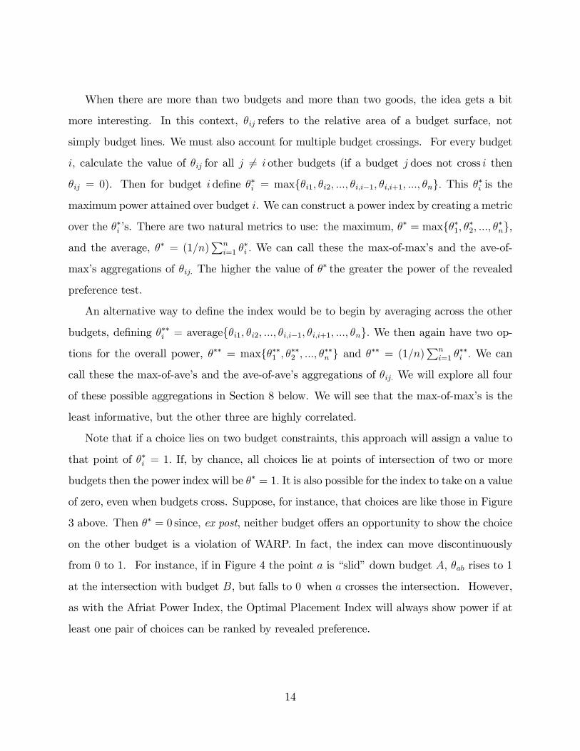
When there are more than two budgets and more than two goods, the idea gets a bit

more interesting. In this context, �ij refers to the relative area of a budget surface, not

simply budget lines. We must also account for multiple budget crossings. For every budget

i, calculate the value of �ij for all j 6= i other budgets (if a budget j does not cross i then

�ij = 0). Then for budget i de�ne ��i = maxf�i1; �i2; :::; �i;i�1; �i;i+1; :::; �ng: This ��i is the

maximum power attained over budget i. We can construct a power index by creating a metric

over the ��i�s. There are two natural metrics to use: the maximum, �� = maxf��1; ��2; :::; ��ng,

and the average, �� = (1=n)Pn

i=1 ��i : We can call these the max-of-max�s and the ave-of-

max�s aggregations of �ij: The higher the value of �� the greater the power of the revealed

preference test.

An alternative way to de�ne the index would be to begin by averaging across the other

budgets, de�ning ���i = averagef�i1; �i2; :::; �i;i�1; �i;i+1; :::; �ng: We then again have two op-

tions for the overall power, ��� = maxf���1 ; ���2 ; :::; ���n g and ��� = (1=n)Pn

i=1 ���i : We can

call these the max-of-ave�s and the ave-of-ave�s aggregations of �ij: We will explore all four

of these possible aggregations in Section 8 below. We will see that the max-of-max�s is the

least informative, but the other three are highly correlated.

Note that if a choice lies on two budget constraints, this approach will assign a value to

that point of ��i = 1: If, by chance, all choices lie at points of intersection of two or more

budgets then the power index will be �� = 1: It is also possible for the index to take on a value

of zero, even when budgets cross. Suppose, for instance, that choices are like those in Figure

3 above. Then �� = 0 since, ex post, neither budget o¤ers an opportunity to show the choice

on the other budget is a violation of WARP. In fact, the index can move discontinuously

from 0 to 1. For instance, if in Figure 4 the point a is �slid�down budget A, �ab rises to 1

at the intersection with budget B, but falls to 0 when a crosses the intersection. However,

as with the Afriat Power Index, the Optimal Placement Index will always show power if at

least one pair of choices can be ranked by revealed preference.

14

This method is similar to the �Sequential Maximum Power� technique of Blundell,

Browning and Crawford (2003). Their analysis was aimed at data with su¢ cient obser-

vations to (nonparametrically) estimate expansion paths. For a given choice, the researcher

can �nd the optimally placed budget, as we use the term above, and then use the expansion

path to project a choice onto this optimal budget. In this way one can construct the optimal

(most powerful) test of GARP using only the optimally placed budgets. If, as they suggest,

estimating expansion paths is possible, then applying their test will give an Optimal Place-

ment Index of 1. However, if there is insu¢ cient data to estimate expansion paths then their

Maximum Power test will be impossible. In this case, the power index presented here gives

us a measure of how close the budgets in the GARP test come to meeting the Blundell,

Browning and Crawford ideal.

5.1 Strengths and Weaknesses of the Optimal Placement Index

A shortcoming of this metric is that it is only operable for WARP, not GARP. When there

are only two goods, WARP is both necessary and su¢ cient for the existence of a well behaved

(strictly convex) preference, so the metric above would su¢ ce. However, for more than two

goods, WARP ceases to be su¢ cient. While it could in principle be generalized to GARP,

the process would be di¢ cult and tedious, with dubious net bene�t. Moreover, with only

two goods it is impossible to have a violation of GARP without also having a violation of

WARP, although this is not the case with more goods. As a result, this power test is more

demanding of the budgets than GARP would require, which will mean that the true power

of the test is likely to be higher than this index might imply.

A second shortcoming of this index is that it only speci�es the optimal placement of

budget constraints for predetermined slopes.7 In this index the slopes of budgets are not

chosen, so neither is the index truly optimal.

Third, there is no natural threshold to indicate when a test has high power, short of

� = 1. At best, therefore, this index can indicate relative degrees of power.

7This is also true of the Blundell, Browning and Crawford (2003) analysis.

15

Finally, there is an unstated assumption that the budget providing the greatest proportion

of itself exposed to a violation of revealed preference is also the most likely to �nd such

a violation. If all goods are normal goods, then this conclusion follows naturally from

Proposition 1 of Blundell, Browning and Crawford (2003). Hence, normality is required

for the optimally placed budgets to maximize power.

6 Jittering

Implicit in the prior two methods is that behavior is measured without error. Next suppose

that there may be an element of randomness to either measurement or behavior. This

measure of power is based on comparing the variation in choices observed to the degree of

randomness necessary to generate violations of GARP.

To motivate this approach, suppose a person was o¤ered the �ve budget constraints

pictured in Figure 5, and all of the choices involved equal quantities of both goods, as in

the left panel of the �gure. These choices do not violate GARP and are consistent with

preferences that have a kink at the 45-degree line, as would Leontief preferences. If we were

to posit a sixth budget we would likely predict that, again, the choice would be on the 45-

degree line. Hence, there appears to be very little randomness to these choices. By the same

token, adding only the slightest shift in choices along the budget constraint (in the right

direction) would result in a GARP violation. Hence, we would like to conclude that this is a

very strong test of rationality� the data shows a great deal of regularity and predictability,

and only the slightest perturbation would result in violations of GARP.

Compare this to the data shown in the right panel of Figure 5. Here the data look as

though they are consistent with a perfect substitutes utility function. However, despite the

relative degree of predictability of the data, there would have to be very big perturbations

added to the data in order to generate violations of revealed preference. Hence, relative to

the left panel, the right panel is a less powerful test of rationality.

16

Figure 5

To formalize these intuitions, we �rst need to de�ne the concept of errors. Restrict all

budget constraints to be linear. Represent each choice as a point xk along the budget line

k of length `k. That is, xk 2 [0; `k]:8 Suppose the true choice is zk but that the researcher

observes xk = zk + "k; where the "k are independently and identically distributed according

to some function f(0; �2):9

Next we need to construct two measures. First is a measure of how much error we need to

add to the data in order to generate a predetermined severity of GARP violations. Second is

a measure of the amount of variance or error occurring naturally in the data. By comparing

the variation we need to add to the naturally occurring variation, we can get an index of

how tightly the model has been tested.

We can get the �rst measure by adding random noise to the observed data. Let ~"k be

draws from the distribution f(0; ~�2) for a speci�ed value of ~�. Let ~zk = xk + ~"k: Then for a

given set of draws ~"we can test the �jittered�data, ~z, for GARP violations.10 For each ~�

8The generalization to budget planes is straightforward. We can think of vector xk as a point on the planewith vector "k drawn from a multivariate distribution. It is important to note that if ther are m goods inthe budget, then both xk and "k are of dimension m� 1:

9The only other case we know of that used this method to get a sense of power was Manser and McDonald(1988). They �repeatedly multiplied all quantities consumed by i.i.d. lognormal psuedo random numberswith unit expectations.�They progressively increased the variance of the lognormal random numbers andmeasured the violations of GARP over 100 simulations. They found standard deviations of 0.10 to 0.20 wereneeded to get signi�cant violations of GARP, which they interpreted as strong power.10Note that the terms �jitter,��jittered data,�and �jitter statistics�are not original to this paper, but

are well-accepted statistical terms. Jittering is commonly used in engineering, for instance.

17

we repeat this exercise for say 10,000 iterations. We can then search for the value of ~� such

that, say, 5% of the jittered experiments �nd at least one GARP violation or have an Afriat

E¢ ciency Index of e� � 0:95 (or some other �critical�value). We can think of this critical

value as that which we would use to reject the rationality of the data when there are errors.

Call the value of ~� that meets the criterion ��. This �� gives us an indication of how close

the chosen budgets came to �nding a violation of rationality� the closer �� is to zero, the

sharper the test of rationality.11

How do we use �� to ask whether the original data provide a powerful test of GARP? A

sensible way is to test whether the noise added to create the jittered data, ~", is signi�cantly

bigger than the noise naturally occurring in the data, ": A test with low signi�cance will

have high power.

Consider a test of the null hypothesis that ~" and " both have the same variance, �2: For

each individual in the sample, consider the statistic

� =

P(xk � ~zk)2=�2P(xk � zk)2=�2

� ��2

�2:

Under the null hypothesis � is characterized by the F distribution. If there are m goods on

each of n budgets, then this F�test has n(m� 1)degrees of freedom in both the numerator

and denominator.12 Let s be the signi�cance level of �: Then one can consider the con�dence

of the test to be 1� s: For instance, if �� � 0; then con�dence in the test approaches 1.

How can we specify the level of natural variance �? This question is reminiscent of that

encountered by Varian (1985) in his goodness-of-�t analysis, and the answers are thus similar.

One option is to �nd a parametric estimate of a utility function and let the standard error

of the regression stand for �. This, obviously, dilutes the value of non-parametric analysis

with parametric analysis. Moreover, there often may be too few observations from a single

11Note that this method even works to �nd power when there are violations of GARP, but just relativelyfew. We may still want to think of performing jittering to see how much noise we need to add to bringviolations up to some critical value.12Recall that we are thinking of x as a point on a budget plane. Thus there are only m� 1 independent

values in the vector x, andm�1 elements in ": Note also that the vector notation implies thatP(xk�zk)2 =Pn

k=1

Pm�1i=1 (xki � zki)2:

18

agent to estimate such a function. We would be left to postulate � from some other ad hoc

means. Alternatively, we could derive the level of natural variance in the data needed to

justify a given level of con�dence. For instance, suppose we would conclude that the power

of the test is insu¢ cient if � > C: Then a � � C would meet the desired level of con�dence.

Let � = ��C�1=2. Then any � � � would be enough natural variance to satisfy the desired

con�dence, and we could appeal to intuitions about whether � is �small.� For example,

suppose we gave a subject 8 budgets of two goods each, found no violations of GARP, and

determined �� = 0:2 would generate a 5% chance of a violation. Suppose we would conclude

that the GARP test is of weak power if � revealed a di¤erence between the variance of ~" and

" at, say, the � � 0:05 signi�cance level. From a F (8; 8)-Distribution table we �nd C = 3:44;

and solving we �nd � = 0:11: This implies that if the natural error in the data is from a

normal distribution of mean zero with standard error of � � 0:11; then we would not reject

the test as lacking in power. If this value of � seems reasonable given the circumstances,

then the researcher can be comfortable with the power of the test.

Applying this to the example given in Figure 5 above, we could easily conclude that in

both cases the level of natural variance is small since the data are so well organized and

conform to an easily estimated utility function. However, in the panel on the left, the tiniest

� will generate violations of GARP (�� � 0 in this case) and the revealed preference test

is passed with con�dence approaching 1. By contrast, the right panel passes but with very

low con�dence. Here � is again close to zero, while �� is going to be above 0.25, making

� extremely high and the required natural variance to be unnaturally large.

6.1 Strengths and Weaknesses of Jittering

The F�test above, as with Varian�s (1985) chi-squared test of goodness-of-�t, has some

distinct costs and bene�ts. The main strength of the approach is the ability to specify a

statistical level of con�dence for a stated �: The main weakness is, obviously, having to

state a � and specify the probability distribution function as normal. Varian answers this

by arguing that conceding a normal distribution is a small sacri�ce compared to a full-blown

19

parametric estimation of utility. Moreover, having to specify a � is tempered by being able

to state a needed � threshold for variance in the data. If � is a number that all would agree

is small given the nature of the data, then arguments over � may be avoided.

7 Bootstrapping Indices for Panel Data

This technique was introduced in Andreoni and Miller (2002) and Harbaugh, Krause, and

Berry (2001). We include it here for completeness.

When there are several measures on a series of subjects, one can ask the question of the

power of the test in a new way. In particular, one can ask whether the organization put on

the data by the subjects themselves� by matching individuals with choices� is superior to

another method that would have randomly assigned choices to individuals from the universe

of choices actually made.

For simplicity, consider an example of two experimental subjects given the same two

budgets. Suppose the data are like that shown in Figure 6. Here there are no violations of

revealed preference. Suppose that, on each budget, we were to pool the choices made by

the subjects and then create new synthetic subjects by randomly drawing from the universe

of choices actually made. That is, we use bootstrapping techniques to generate a measure

of power. In the example of Figure 6, x1 2 fa; dg, and x2 2 fb; cg: Then there would be a

25% chance that the synthetic subject would be assigned choices a and c; hence violating

GARP, which is the maximum likelihood possible with two budgets and no initial violations

of revealed preferences.

20

a

c

d

b

Figure 6

Compare these choices to those in Figure 7. Here there would be no chance that we could

create a synthetic subject that would violate GARP. In this sense, the test has more power

if the study generates data like that in Figure 6 rather than Figure 7.

a

c

d

b

Figure 7

Note that this technique can report either greater or lesser power than a simple Bronars

method of randomly assigned choices along budgets. For instance, in the budgets shown

in Figures 6 and 7 a Bronars (Monte Carlo) test would show only about 12% of the cases

�nding violations, whereas the bootstrapping test will get exactly 25% violations (Figure 6)

or 0% violations (Figure 7).

We can now specify as the alternative hypothesis that the full sample of choices on

each budget is the population and that choices along a budget were chosen from this set at

21

random, with replacement. With this alternative, the probability of violations among the

synthetic subjects is the power of the test.

7.1 Strengths and Weaknesses of Bootstrapping Methods

The main strength of this panel bootstrapping technique as compared to, say, Bronars�

method, is that by treating the sample as the universe it reveals how well the test was suited

to the population studied, and whether the test was indeed successful in generating enough

variation in choices to make violations of GARP a credible possibility. This power index

is particularly well suited to experiments with large numbers of subjects. Like the Bronars

method, however, the alternative hypothesis speci�ed is still likely to ascribe too much

randomness to each subject, especially in very heterogeneous populations of experimental

subjects.

8 Application to Experimental Data

In this section the indices described above will be applied to an experimental data set. The

data employed are described in detail in Andreoni and Miller (2002) and Andreoni and

Vesterlund (2001). Brie�y, the experiment was designed to explore individual preferences

for altruism by asking subjects to make a series of choices in a Dictator game, under varying

incomes and costs of giving money to another subject. In particular, subjects made eight

choices by �lling in the blanks in statements like this: �Divide M tokens: Hold at X

points, and Pass at Y points (the Hold and Pass amounts must sum toM),�where the

parametersM , X; and Y were varied across decisions. The subject making the choice would

receive the �Hold�amount times X, and another subject would receive the �Pass�amount

times Y . All points were worth $0.10.

22

0

50

100

150

100 150

0

50

payment to self

pay

men

t to

 oth

er

0

50

100

150

100 150

0

50

payment to self

pay

men

t to

 oth

er

Figure 8: Andreoni and Miller (2002) budgets

Let �s be payo¤ to self, and �o be payo¤ to other. The hypothesis is that individuals

have well-behaved preferences Us = U(�s; �o):The experimental parameters imply a budget

constraint for any choice of1

X�s +

1

Y�o =M:

The parameters chosen provided the budgets shown in Figure 8. As can be seen, the pie to

be divided ranged from $4 to $15 and the relative prices ranged from 3 to 1/3. After subjects

made all 8 choices, one choice was selected at random by the experimenter and carried out.

Data was collected on 142 subjects and each subject�s choices were tested for violations of

GARP.13 The result was that 13 of the subjects (9.1%) had violations of GARP. Applying the

Afriat E¢ ciency Index, only 3 of these were found to be large violations (as we show below).

This is a rather striking failure to contradict the neoclassical model of preferences, but

leaves open the question of how discriminating the GARP test was at uncovering potential

13Andreoni and Miller (2002) report data on 176 subjects, but their session 5 is set aside here for brevity.

23

violations.14 We consider the indices provided above, starting with the Bronars Index.

Bronars Index. Taking one million random draws from a uniform distribution on each

of the eight budget sets, we found 0.78 of all Monte Carlo experiments resulted in at least

one violation of GARP. Under this alternative hypothesis, Bronars�Method 1 has a modest

degree of power. His Method 2, with random budget shares, fares worse, with a power of

only 0.63. Method 3 is still worse, with a power of only 0.48. This illustrates the sensitivity

of the power test to the alternative hypothesis.

Afriat Con�dence Index. Table 1 shows the frequency of Afriat Con�dence Indices,

Ai, for all 142 subjects. The top of the table shows the 13 subjects who violated GARP at

least once, and the bottom shows the 129 who had no violations. Nine of the 13 violators had

Afriat Con�dence Indices of 1, indicating that the smallest change in choices would remove

all violations of GARP. One subject had an Afriat Con�dence Index of 0.98, which is within

the threshold setting of 0.95. Three of the 13 had severe violations beyond this threshold.

How about the 129 subjects who showed no violations? More than two-thirds of these

(71%) had Afriat Con�dence Indices of 1, indicating that the GARP test could not have been

sharper. If we apply the same criterion for �high power� that we do to �small violation�

then 107 (83%) of the non-violators have Ai � 1:05. Then the �con�dence interval�of Afriat

Con�dence Indices such that 0:95 � Ai � 1:05 includes 117 subjects. In sum, this means

that 82.4% of subjects were given stringent tests of GARP and passed, 2.1% of subjects had

signi�cant violations of GARP (Ai < 0:95) and 15.5% were given GARP tests that were not

su¢ ciently diagnostic (1:05 < Ai). Using the most stringent con�dence interval, Ai = 1;we

�nd 73.2% of subjects passed the strongest possible test.

14Andreoni and Miller (2002) reported both the Bronars Method 1 power index and the panel index. Werepeat them here for completeness.

24

Table 1Afriat Confidence Indices, Ai

Ai Frequency PercentViolation of GARP: 0.83 1 0.70

0.92 2 1.410.98 1 0.701.00 9 6.34

No Violation: 1.00 95 66.901.01 2 1.411.02 1 0.701.03 3 2.111.04 6 4.231.07 4 2.821.08 10 7.041.10 1 0.701.13 2 1.411.14 1 0.701.15 1 0.701.17 3 2.11

Total: 142 100.00

Optimal Placement Index. There were four ways proposed to report this index. The

�rst two begin by �nding the maximum measure for each budget, with 1 being the ideal, and

then either �nd the maximum across budgets (Max of Max�s) or the average across budgets

(Ave of Max�s). The next two begin by averaging the power provided by all other budgets,

and then �nd the maximum across budgets (Max of Ave�s) or the average across budgets

(Ave of Ave�s).

Table 2 shows the results from the Optimal Placement Index. The Max of Max�s measure

reveals that 95% of subjects were, at some point in the study, given a most powerful test

at least one time. The lowest Max of Max�s index, � = 0:75; indicates that the most

powerful test this subject faced was 75% as powerful as the most powerful test available.

The obvious problem with the Max of Max�s measure is that it only identi�es the best test

faced by the subject. The remaining three columns indicate that this is hiding a great deal of

25

heterogeneity across subjects in the power they faced. Here we are confronted directly with

the fact that this index does not give us a speci�c criterion for high or low power. Compare

the Max of Max�s to the Ave of Ave�s, for instance. One gives the impression of very high

power, but the other of very low power, yet they are simply di¤erent ways of aggregating

the same power measure.Table 2

Optimal Placement IndexMax of Max�s Ave of Max�s Max of Ave�s Ave of Ave�s

Range� Freq. % Freq. % Freq. % Freq. %95�100 135 95.1 24 16.990�95 1 0.785�90 3 2.1 4 2.880�85 1 0.7 3 2.175�80 3 2.1 8 5.670�75 6 4.265�70 7 4.960�65 13 9.255�60 2 1.450�55 50 35.245�50 5 3.5 57 40.140�45 8 5.6 1 0.735�40 6 4.230�35 2 1.4 44 31.0 24 16.925�30 2 1.4 27 19.0 2 1.420�25 10 7.0 13 9.215�20 1 0.7 24 16.910�15 3 2.1 66 46.55�10 11 7.70�5 2 1.4

Total 142 100 142 100 142 100 142 100*Each range category includes the upper but not the lower element.

Jittering. There are two obvious ways of specifying the error distribution to jitter the

data. First is to de�ne the standard error in proportion to the length of the budget line

(~�i = ~�`i), which we call relative errors. The second is to let the distribution be the same

for all budgets regardless of length (~�i = ~�), which we call absolute errors. In both cases we

26

use a truncated normal distribution.15 After we add the jitters we can then �nd the critical

amount of natural variance in the data, �, such that the jittered data would fail the F -test

at the 95% con�dence interval. If the natural error in the data is above �, then we can

believe the test had power of at least 0.95.

Figure 9 shows the values of � for all 129 subjects who had no violations of GARP. The

bars are the marginal density and the lines are the cumulative density. Panel a shows that,

under relative errors, if the natural error in the data exceeds �i = 0:08`i; then 90% of the

subjects would have been given signi�cantly powerful tests of GARP. Panel b shows that,

under absolute error, a similar degree of power holds if the natural error exceeds � = 10.

This leads naturally to the question, how much natural error exists in the data? Looking

at the data, one sees immediately that one source of natural error is rounding. Perhaps for

cognitive ease, subjects have an overwhelming tendency to choose numbers divisible by 10.

This is true for both the hold and pass amounts. In fact over 85% of all choices had both

the hold and pass values divisible by 10. Another 11% were divisible by 5, but not 10. Only

4% of choices made were not divisible by either 10 or 5.

15We also considered censored errors, where the ends of the budget constraints absorbed the extra variance.The results are similar and, for brevity, are not presented.

27

0

10

20

30

40

50

60

70

80

90

100

0 0.01 0.02 0.03 0.04 0.05 0.06 0.07 0.08 0.09 0.10 0.11 0.12 0.13

Standard  Error

Percent

Marginal

Cumulative

a. Critical � for Relative Error (~�i = ~�`i):

0

10

20

30

40

50

60

70

80

90

100

0 1 2 3 4 5 6 7 8 9 10 11 12 13 14 15 16 17 18

Standard  Error

Percent

b. Critical � for Absolute Errors (~�i = ~�)Figure 9: Critical Values of Natural Error

for 95% Confidence on Jittered Data:

28

Suppose we assume subjects restrict choices to those where both hold and pass amounts

are divisible by 10, and that �rational rounding� would choose the point that yields the

highest utility.16 This means that the maximum error would be at least 5, assuming con-

vex preferences. To be conservative, therefore, assume a uniform distribution of absolute

rounding errors between 0 and 5, and thus an expected absolute error of 2.5 tokens. We

can calculate what this means for "i. Under the assumption of relative errors,17 this implies

E j"ij = 0:43. For absolute errors this implies of E j"ij = 5:7: It is easy to show that our

assumptions imply the standard error18 of � � 1:15Ej"ij: For the assumption of relative

errors, this means �i = 0:049, while for absolute errors it means �i = 6:53: As a result,

rounding errors alone would provide enough natural variance in the data to make at least

38% of our GARP tests have su¢ cient power. If we were to believe that there is some other

independent variation in the data (either from measurement, reporting or learning) that is

roughly equal to noise from rounding, so the expected absolute error was about 5 tokens on

each budget, then �i � 0:1 for relative and �i � 13 for absolute errors. If this were the case,

then about 95% of the GARP tests would have su¢ cient power.

Bootstrapping. Since the experimental data set here is actually a panel, we can use

the panel techniques to measure the power of the test. On each of the eight budgets there

are 142 observations. We conducted one million Monte Carlo experiments where we took

one draw from the 142 observations on each budget to form a synthetic subject. Of the

million synthetic subjects drawn, 76.6% had at least one violation of GARP. This is very

close to the power found from Bronars�Method 1 which assumed purely random draws from

a uniform distribution of choices. However, the power from the Panel approach far exceeds

the power from Bronars�Methods 2 and 3.

16This need not hold at the corners of the budget set where, for instance, holding all 75 tokens might beoptimal.17Budgets range in length from 85 to 167. The average length of a budget constraint is 135.18Assume �a � "i � a: Then by symmetry Ej"ij =

R a�a j"ij

12ad" =

R a0"i1ad" = a=2: Also, �

2i = E("

2i ) =

a2=3: Combining these gives �2 = 4Ej"ij2=3:

29

9 Correlations Across Indices

Since the indices presented above are attempting to measure the same thing, we also cal-

culated the correlations across the various measures. Table 3 shows the correlations across

subjects. This presents the correlations for only the case that GARP was not violated. The

reason is that the Afriat Con�dence Index is not monotonic, hence correlations using all data

would tend to dampen correlations. Nonetheless, all correlations are nearly identical when

all observations are used.

The �rst thing to notice form Table 3 is that the two most blunt indices, the Afriat

Con�dence Index and the Max of Max�s, are very weakly correlated with all other measures.

By contrast, the remaining �ve indices are extremely highly correlated. Perhaps most com-

forting is that Jittering and the Optimal Placement measures (other than Max of Max�s)

are very highly correlated, with correlations of 0.74�0.84. In particular, this gives con�dence

that Jittering� the most parametric but most statistically precise index� is measuring the

same thing that the Optimal Placement Index� the most intuitive but statistically imprecise

index� is measuring.

Table 3Absolute Correlations Across Power Indices,

Only When GARP is Not ViolatedAfriat Optimal Placement Index Jittering

Con�dence Max of Ave of Max of Ave of �Index Max�s Max�s Ave�s Ave�s relative

Afriat Con�dence 1OPI� Max of Max�s 0:221 1OPI Ave of Max�s 0:194 0:337 1OPI Max of Ave�s 0:168 0:295 0:763 1OPI Ave of Ave�s 0:284 0:242 0:950 0:811 1Jittering � relative 0:132 0:103 0:831 0:739 0:835 1Jittering � absolute 0:202 0:112 0:802 0:747 0:831 0:990� OPI stands for Optimal Placement Index

30

10 Discussion and Conclusion

The objective of this paper was to formally present, analyze, and compare four new ap-

proaches to measuring the power of revealed preference tests. The most straightforward

approach inverts the well-known Afriat E¢ ciency Index into the Afriat Power Index. This

power index, however, su¤ers from being a blunt instrument in the same way the e¢ ciency

index is an imprecise measure of goodness of �t. Nonetheless, it seems both natural and

simple to report the Afriat Power Index alongside the Afriat E¢ ciency Index in any study,

as the Afriat Con�dence Index.

The most intuitive index proposed is the Optimal Placement Index. By allowing �20-

20 hindsight� to the economist, it asks how well the experimental instrument performed

relative to the best possible instrument that could have been dynamically generated after

each choice. The intuitive appeal of this metric is tempered by the fact that it does not

produce clear guidance on power or a natural threshold to appeal to as �high power.� In

short, the approach is �too non-parametric.�

The Jittering method concedes this by adding a modicum of structure. If, for instance,

we assume errors are normally distributed, then we can use an F -test to conclude whether the

revealed preference test was su¢ ciently �close�to �nding a violation of rationality if it were

present. This test is the least transparent of those presented, and far less transparent than

the Optimal Placement Index. However, when all the tests were applied to experimental

data, the correlation between Jittering and the Optimal Placement Index was extremely high.

This indicates that both the transparent and the opaque techniques are measuring the same

thing, and suggests little is compromised� and potentially much gained� by assuming a

parametric model of errors.

The �nal metric presented, Bootstrapping Power, �nds the power of the revealed prefer-

ence test over a full sample, not an individual subject, when there are repeated measures.

It asks whether the organization put on the observations by the subjects is superior to that

of randomly reassigning and remixing subjects�choices. This has an advantage over prior

31

measures by relying on the actual sample of choices to generate the alternative hypothesis,

rather than imposing, for instance, a uniform distribution across the entire budget set.

In sum, whether using survey or experimental data, the tension between goodness-of-�t

and power is clear in revealed preference tests. In this paper we hope to have provided some

guidance to researchers to both design and analyze tests that maximize our ability to make

the correct inferences about economic models of maximizing behavior.

32

ReferencesAfriat, Sidney (1967): �The Construction of a Utility Function From Expenditure Data,�

International Economic Review, 8, 67-77.

Afriat, Sidney (1972): �E¢ ciency Estimates of Production Functions,�International Economic

Review, 13, 568�598.

Aizcorbe, Ana M. (1991): �A Lower Bound for the Power of Nonparametric Tests,�Journal of

Business and Economic Statistics, 9, 463�467.

Andreoni, James and John H. Miller (2002): �Giving According to GARP: An Experimental

Test of the Consistency of Preferences for Altruism,�Econometrica, 70 (2), 737�753.

Andreoni, James and Lise Vesterlund (2001): �Which is the Fair Sex? Gender Di¤erences in

Altruism,�Quarterly Journal of Economics, 116, 293�312.

Battalio, Raymond C., John H. Kagel, Robin C. Winkler, Edwin B. Fisher, Robert L. Bas-

mann, and Leonard Krasner. �A Test Of Consumer Demand Theory Using Observations Of

Individual Consumer Purchases,�Western Economic Journal, 11(4), 411�28.

Becker, Gary S. (1962): �Irrational Behavior in Economic Theory,�Journal of Political Econ-

omy, 70, 1�13.

Blundell, Richard W., Martin Browning, and Ian A. Crawford (2003): �Nonparametric Engel

Curves and Revealed Preference,�Econometrica, 71, 208�240.

Bronars, Stephen G. (1987): �The Power of Nonparametric Tests of Preference Maximization,�

Econometrica, 55 (3), 693�698.

Cox, James C. (1997): �On Testing the Utility Hypothesis,�The Economic Journal, 107, 1054�

1078.

Famulari, Melissa (1995): �A Household-Based, Nonparametric Test of Demand Theory,�Re-

view of Economics and Statistics, 77, 372�382.

Février, Philippe and Michael Visser (2004): �A Study of Consumer Behavior Using Laboratory

Data,�Experimental Economics, 7, 93�114.

33

Harbaugh, William T., Kate Krause, and Tim Berry (2001): �GARP for Kids: On the Devel-

opment of Rational Choice Behavior,�American Economic Review, 91, 1539�1545.

Houthakker, Hendrik (1950): �Revealed Preference and the Utility Function,�Econometrica,

17, 159�174.

Manser, Marilyn E. and Richard J. McDonald (1988): �An Analysis of Substitution Bias in

Measuring In�ation, 1959-1985,�Econometrica, 56, 909�930.

Mattei, Aurelio (2000): �Full-Scale Real Tests of Consumer Behavior Using Expenditure Data,�

Journal of Economic Behavior and Organization, 43, 487�497.

Samuelson, Paul A. (1938): �A Note on the Pure Theory of Consumer Behavior,: Econometrica,

5, 61�71.

Sippel, Reinhard (1997): �An Experiment on the Pure Theory of Consumer�s Behavior,�The

Economic Journal, 107, 1431�1444.

Varian, Hal R. (1982): �The Nonparametric Approach to Demand Analysis,�Econometrica,

50, 945-973.

Varian, Hal R. (1983): �Nonparametric Test of Models of Consumer Behavior,� Review of

Economic Studies, 50, 99�110.

Varian, Hal R. (1984): �The Nonparametric Approach to Production Analysis,�Econometrica,

52, 579�597.

Varian, Hal R. (1985): �Non-Parametric Analysis of Optimizing Behavior with Measurement

Error,�Journal of Econometrics, 30, 445�458.

Varian, Hal R. (1990): �Goodness-of-Fit in Optimizing Models,�Journal of Econometrics, 46,

125�140.

Varian, Hal R. (1991): �Goodness of Fit for Revealed Preference Tests.�University of Michigan

CREST Working Paper Number 13.

34