poverty and vulnerability dynamics: empirical - agecon search

Quarterly Journal of International Agriculture 51 (2012), No. 4: 301-332

Quarterly Journal of International Agriculture 51 (2012), No. 4; DLG-Verlag Frankfurt/M.

Poverty and Vulnerability Dynamics: Empirical Evidence from Smallholders in

Northern Highlands of Ethiopia

Abrham Seyoum Tsehay and Siegfried Bauer Justus-Liebig-University Gießen, Germany

Abstract

This study is primarily intended to examine the dynamics and determinants of rural household poverty and vulnerability in Northern Highlands of Ethiopia. Besides, it compares the result of asset-based poverty measurement against the standard consumption-based approach between two purposively selected Peasant Associations (PAs) in the region. The data for this research emanated mainly from the Ethiopian Household Survey (ERHS). Substantial improvements in many of the measures of household’s welfare (in terms of selected data on assets, education and participation in development activities) have been observed over the study period. However, considerable proportion of households is found to be poor and vulnerable in both PAs. In addition, the trends of both measures have been found to vary between the peasant associations. Moreover, the consumption based approach shows lower poverty incidences in shumsheha in all the survey rounds compared to Yetemen contrary to the results of the PCA approach, which appears to second previous village studies. This indicates the limitation of the consumption based approach in accounting for over all changes in the wellbeing of households. The study also compared the different determining factors of poverty and vulnerability in the two PAs and important implications drawn from the results are discussed.

Keywords: poverty dynamics, vulnerability, rural Ethiopia JEL: I32, R20

1 Introduction

Several studies have been measuring poverty by employing income or consumption expenditure as proxy for the living standard of individuals or households against a certain minimal accepted threshold. This approach has been considered as the standard approach, which has been effectively used in raising public concern for poverty thereby guiding policy action (BOOYSEN et al., 2005; BRANDOLINI et al., 2009, and BRANDOLINI et al., 2010). Yet, it is not without shortcomings. First, income fails to represent the full amount of available resources, as individuals can also rely on real

302 Abrham Seyoum Tsehay and Siegfried Bauer


and financial assets to cope with the needs of everyday life and to face unexpected events. A second, more radical, critique of the income inadequacy approach is that income is only a means and not an end in itself. As such, it cannot account for the multiple dimensions of human well-being (BRANDOLINI et al., 2010). Moreover, based on flow variables and informant recall, income-based poverty indicators are more prone to measurement errors than are indicators based on visible assets such as land or livestock (WOOLDRIDGE, 2002).

In response to the above-mentioned shortcomings of the conventional approach, the measurement of poverty has been broadened over the years to incorporate different aspects of human wellbeing. These include a number of alternative approaches such as, for instance, those that employ various other socio-economic indicators to measure poverty. Of these alternative or multidimensional approaches to the measurement of poverty, the asset index approach applied to data from demographic and health survey has gained increasing popularity in recent years (FILMER and PRITCHETT, 1998; SAHN and STIFEL, 2000; WORLD BANK, 2012, and BOOYSEN et al., 2005).

Guided by evidences emanated from such measurements, policy interventions in many of the developing world have been generally steered by the fundamental goal of poverty reduction. Typically, these policies are often based more on ex-post poverty incidences rather than ex-ante predictions. However, a household’s current poverty may be a bad guide to its future prospects explains the recent emphasis in the poverty literature on vulnerability, a forward-looking poverty concept (WORLD BANK, 2001).

Like that of many countries in sub-Sahara Africa, poverty is pervasive and vulnerability is widespread in Ethiopia. This has attracted several studies on poverty and food insecurity in the country mainly based on cross-sectional data over the past couple of decades. Nonetheless, most of the studies conducted so far applied the conventional income-based measurements of poverty, which share shortcomings of the standard poverty measurement approach (HAGOS and HOLDEN, 2003; KEDIR and MCKAY, 2003; ISLAM and SHIMELES, 2007; BIGSTEN and SHIMELES, 2008; and DERCON et al., 2011). One notable exception in this regard is LIVERPOOL and NELSON (2010). The study compared asset-based and consumption-based poverty measurements using panel data from rural Ethiopia for six rounds from 1994 to 2004. Against the backdrop of the aforementioned limitations, this study aims at analyzing the trends and deter-minants of poverty in two purposively selected Peasant Associations (PAs) in northern highlands of Ethiopia for four rounds from 1994 and 2010. The major departure of this study from the previous ones is that it uses an asset-based approach and attempts to compare it with the results of the consumption based approach. In a nutshell, this study differs from earlier studies in three important aspects. First, it adds into the panel data a recent survey round for 2010. Second, it uses Principal Component Analysis (PCA)

Poverty and Vulnerability Dynamics 303


to develop the asset index as opposed to regression-based approach done by LIVERPOOL and NELSON (2010). Third, it supplements the results of the ex-post poverty measurements by ex-ante predictions of poverty and quests to unravel the determining factors behind the trend.

The rest of the paper is organized as follows. It starts with a brief description of the data used and the methodological approach applied. It then presents the description and the expected signs of the explanatory variables employed in the regression models followed by descriptive statistics and econometric analysis of the dynamics and determinants of poverty and vulnerability in Northern highlands of Ethiopia. Finally, the paper concludes with some relevant policy implications.

2 Data and Research Methods

2.1 Data

The data for this research were generated mainly from the Ethiopian Rural Household Survey (ERHS), a rich panel data set conducted by Department of Economics (Addis Ababa University) in collaboration with International Food Policy Research Institute (IFPRI) and Center for the Study of African Economies (CSAE - University of Oxford) since 1994. Besides, primary data were collected tracing the panel of households of ERHS in two Peasant Associations (PAs) - the smallest unit of administration in the former regime and constitutes of roughly 1,000 households of Northern Ethiopia in 2010. This study, therefore, constituted two PAs in northern highlands of Ethiopia, namely Yetmen and Shumsheha. Yetmen, which constitutes 8 villages, symbolizes the high rainfall, fertile arable land, grain dominated and relatively rich parts of region, while Shumsheha constitutes 10 villages and represents the semi-arid, insufficient rainfall, limited arable land, cereal growing and vulnerable parts of the region. The study considered a total of 209 households; 61 from Yetmen and 148 from Shumsheha. The attrition rate is only 13.88 % in 16 years panel data (which means 0.93 % attrition rate per year). Though the sample is not representative of the northern highlands of Ethiopia, it could give a pretty good agro-ecological representation in the region.

2.2 Research Methods

The research methods used in this article are presented in three sections. The first part deals with the measurement of poverty dynamics in the region using both consumption-based and asset-based approaches. Second, three steps Feasible Generalized Least Squares (FGLS) is employed to analyze the vulnerability of rural households to



poverty. Finally, fixed effects instrumental variable (FEIV) and multinomial logit models (MNL) are used to identify factors determining poverty and vulnerability to poverty. A brief description is provided below on the respective models employed in this study.

2.2.1 Poverty Dynamics and Decomposition

(A) Poverty Dynamics

Given the panel data described in the preceding section, an attempt was made to compare consumption-based approach of poverty estimations with asset based approach as given below.

(i) Consumption-based Approach

In this approach, households are deemed to be poor if their real monthly consumption expenditure per adult equivalent is less than 57.6 Ethiopian Birr (ETB) or 30 US dollars in 1994 Purchasing Power Parity (PPP) prices. To put it precisely, the poverty threshold is 1 USD per adult per day in 1994 PPP prices, which is equivalent to 1.92 ETB per adult per day. Using this cut off point, the trend of poverty incidence over the panel years is examined in absolute terms.

(ii) Asset-based Approach

The alternative approach is to develop relative poverty indices for the panel years using Principal Component Approach (PCA). PCA is a mathematical procedure that uses an orthogonal transformation to convert a set of observations of possibly correlated variables into a set of values of linearly uncorrelated variables called principal components. Variables that are correlated with one another, possibly because they are measuring the same construct are reduced to a smaller number of principle components.

In developing the index, variables related to the factors that are explicitly considered as factors of poverty are taken to develop the index driven by previous literature in the area. Accordingly, several variables representing different dimensions of poverty are included given limitations of data. These factors fall into one of the forms of capital: human, natural, physical, social and financial capital. Thus, the principal component used is a function of all of these factors, which is specified as follows:

(1) naturalcapital, physicalcapital, humancapital,socialcapital financialcapital

A principal component is a linear combination of optimally-weighted observed variables. Accordingly, principle principal component analysis is used to reduce the



variables to one composite index called asset poverty index. In the course of performing a principal component analysis, it is possible to calculate a score for each variable on a given principal component. Below is the general form for the formula to compute scores on the first component extracted in a principal component analysis.

(2) ⋯

Where represents the score on principal component 1 (the first component extracted), is the regression coefficient (or weight) for observed variable p, as used in creating principal component 1 and refers to the value of observed variable p.

The regression weights are determined by using a special type of equation called an eigen equation. The weights produced by these eigen equations are optimal weights in the sense that, for a given set of data, no other set of weights could produce a set of components that are more successful in accounting for variance in the observed variables. The weights are created so as to satisfy a principle of least squares similar (but not identical) to the principle of least squares used in multiple regression.

Similarly, principal components are extracted equal to the number of observed variables being analyzed. However, in most analyses, only the first few components account for meaningful amounts of variance. So, only these first few components are retained, interpreted, and used in subsequent analyses (such as in multiple regression analyses). When the eigen value is greater than one, those principal components are extracted. The first component extracted in a principal component analysis accounts for a maximal amount of total variance in the observed variables. Once the first component is identified, it is possible to calculate the vulnerability to poverty index for each household as follows:

(3) ∑

Where is the asset poverty index for household j, is the weight of the ith variable in the PCA represented by the factor score, refers to the value of ith variable for the jth household standardized by the mean, , and standard deviations, , of variable from over all households. By construction, the mean value of the poverty index is zero. To facilitate the index’s comparability over the rounds, the innovative approach of CAVATASSI et al. (2004) was employed. Accordingly, the data for the four survey rounds were pooled and the principal components over the combined data were estimated. The resulting weight is then applied to the variable values for each round of the data using equation 3 above.



(B) Poverty Decomposition

The spells and components approach are the most widely used methods of poverty dynamics and decomposition. In this paper, both approaches are used but emphasize is given to the latter approach, which has advantage over the former in terms of capturing information about the position of households’ consumption expenditure relative to the poverty threshold. The discussion starts with a brief description of components approach, which was developed by RODGERS and RODGERS (1993) and used by JALAN and RAVALLION (2000). JALAN and RAVALLION (2000) decomposed household poverty in to chronic and transient components using panel data. A household is in chronic poverty when its inter-temporal mean consumption is below the poverty line. The mathematical presentation of the method is presented below.

The contribution of household i to total poverty is defined as:

(4) , , … ,

Where are the consumption expenditures of household i at time t, and there are T times in which it is measured and is some well-defined poverty measure. We use the familiar Foster-Greer-Thorbecke (FGT) measure because of its additive decomposability property. Thus, total household poverty over the period is measured as the inter-temporal mean of the poverty measure.

(5) ̅ ∑

Where, p is the mean of the FGT measure between the total poverty and T is the number of years. Hence, chronic poverty is measured by

(6) ∗ ∑ ∗ ; 0

Where, Z is the poverty line, y is the mean consumption expenditure of household i, m* is the number of households below the poverty line and n is the number of households in the sample. is a positive parameter, which gives more weight for the poor when it increases. The most common values of are 0, 1 and 2.

Transient poverty (p ) is the difference of total poverty (p ) and chronic poverty (P*). Hence, once chronic poverty is measured, it would be simple to find transient poverty as:

(7) p p p∗ The components approach is complimented by the spells approach for explaining the nature of poverty dynamics in the region. The spells approach involves identifying the



poverty status of a household in the different time periods under investigation. A tool used for this type of analysis is the transition matrix. It is constructed by classifying households’ incomes into different groups. This matrix provides information on the proportion or number that move from one state of poverty to another. The rows of the matrix add up to unity or 100% (ODURU et al., 2003). Transition matrices also give information on transient and chronic poverty based on the households’ length or spells in poverty. The transient poor in this approach is defined as those households that have income or consumption above the designated poverty line in at least one period out of the periods the welfare indicator is measured. The chronic poor have their welfare measure below the poverty line in all the periods (MCCULLOCH and BAULCH, 2002). However, in this paper, following FOSTER (2007), households are considered to be in chronic poverty if they are under poverty line in half or more of the survey rounds. Once the transition matrix is developed, it is easy to note poverty dynamics by using the Shorrocks mobility index, which is presented as follows.

The mobility index, M, for a transition matrix, P, is give as:

(8) M P

Where, trace P is the trace of the transition matrix P, n is the number of states, for example quartiles or deciles. The index is normalized to take a value between 0 and 1 by dividing it by - .

The closer the Shorrocks mobility index to 1 implies the existence

of higher mobility.

2.2.2 Determinants of Poverty

An analysis of poverty will not be complete without explaining why people are poor and remain poor over time. Hence, an appropriate approach would be to analyze the impacts of household characteristics, village level factors, and policy related variables on the welfare of individuals or households using regression-based models at least at micro level. Two types of models are used for this purpose.

The first model employed for this purpose is the fixed effects instrumental variable regression model (FE IV). It has advantage over the random effects model, as it controls unobserved heterogeneities among households. It is formulated as follows:

(9)

(10) , , , 1,2, … , ; 1,2, … ,

Equation 9 is original fixed effects model using log of real consumption expenditure per adult equivalent, , or the asset poverty index as a dependent variable against a



set of identified endogenous variables, , exogenous variables, , period dummies,

, and unobserved household fixed effects, . In equation 10, we regress the endogenous variables against the rest of the variables in the system in addition to set of instrumental variables, , to estimate their predicted values. The predicted values of

the endogenous variables and their lagged values are used as instruments in equation 9. and are idiosyncratic error terms in the respected equations.

The second model used in this study is the Multinomial Logit model for analyzing the factors affecting the probability that a household is in chronic poverty as compared to transient poverty or being non-poor. One of the main advantages of such an approach is ease of specification (GLEWWE and HALL, 1995; GROOTAERT and KANBUR, 1995). However, the main drawback is that it imposes the property of Independence of Irrelevant Alternatives (IIA). Once the data fulfill this property then the model will be appropriate to use.

In the model used in this paper, the regressand takes the values of 0, 1, or 2 depending on whether the household was respectively never poor, poor in one of the rounds, or poor in 2 or more of the rounds. The multinomial logit regression gives the coefficient values for two groups relative to the third omitted group (here the never poor). However, the results are more easily interpreted in terms of the marginal effects and their significance. These show the impact of each explanatory variable on the likelihood of a household being in each one of the three groups.

In this paper, household consumption expenditure is used as a welfare measure for computing poverty. But as in the case of any other welfare indicator, the poverty level computed using consumption expenditure can be affected by measurement errors. However, using the ERHS panel data BIGSTEN and SHIMELES (2008) proved that consumption based mobility estimates are not seriously distorted by measurement errors.

The dependent variable of the model can take one of three discrete values indicating the poverty status of a household (non-poor, transient poor and chronically poor). The probability (P ) that a household i is in a particular poverty state j is modeled as a function of explanatory variables X as follows:

(11) ∑ 0,1,2

Where, β represents a vector of coefficients, β is set to 0, and j can take the values 0 (non-poor), 1 (transient poor) and 2 (chronically poor). The non-poor state (j = 0) is used as the base category in the regressions based on the equation above.



2.2.3 Vulnerability to Poverty

The other major inquisition of this article is to supplement the results of poverty incidences with the ex-ante probability of households being poor using three steps feasible generalized least squares. Linking poverty studies with that of vulnerability to poverty serves as a tool for poverty reduction strategies to attain their goals better. The approach is rooted in the pioneer work of CHAUDHURI et al. (2002). Assuming consumption expenditure to follow a log-normal distribution and the consumption of household i in period t is determined by a set of variables X .

(12) ln And, the variance of the unexplained part of households’ consumption e is also assumed to be a function of the same explanatory variables used in model 12 as follows:

(13) Then equations (12) and (13) are estimated using three-step feasible generalized least squares (FGLS) suggested by AMEMIYA (1977) cited in CHAUDHURI et al. (2002). Then, using consistent and asymptotically efficient estimators β and θ, which are obtained from equations 12 and 13, the following equations are derived:

(14) ⁄ (15) ⁄ Hence, using the estimated expected mean and variance of log consumption in equation (14) and (15) above respectively, the estimated vulnerability to poverty is given as:

(16) | , Φ ̂ Where Φ . denotes the cumulative density of the standard normal distribution function. The estimated values of the vulnerability to poverty index,v , ranges from 0 to 1. Finally, the vulnerability status of households is evaluated using the standard vulnerability threshold of 0.5.

In addition to this, the determining factors of vulnerability to poverty are assessed using fixed effects IV model as in section 2.2.2 except that the dependent variable is now the vulnerability to poverty index. The vulnerability indices found from the results of the above model are regressed against household characteristics, village characteristics, and policy related variables.



3 Definition and Hypothesis of Variables

Based on theoretical expositions and previous empirical studies, the following ex-planatory variables are hypothesized to influence the welfare of households as follows. Annual real consumption expenditure per adult equivalent, asset-based poverty index and vulnerability to poverty index are the dependent variables in the fixed effects instrumental variable regression models, while a categorical dependent variable of being chronic poor, transient poor and non-poor is used in the multinomial logit model.

Gender of household head: the gender of household heads is vital in the context of rural Ethiopia since access to vital resources and decision making capabilities are highly biased against female household heads. In addition to this, female-headed households are usually formed in rural Ethiopia when the male counterpart dies or looses functionality due to old age. In this analysis, it is included as a dummy regressor whereby male-headed households are given 1; otherwise 0. This variable is expected to be negatively correlated with poverty and vulnerability of households.

Age and Age Squared of the household head: age and age squared (a proxy for experience or old age) are expected to be positively and negatively associated with welfare of households in the respective order as aged household heads face a decline in labour supply and decision making capability.

Literacy of the household head: it is a proxy for the education level of the household head and is hypothesized to have a positive impact on the welfare of households.

Household size: its impact on the welfare of households is mixed as shown in previous empirical literature. It is expected to affect the dependent variable either ways depending on the demographic composition of the household. Its effect will be positive if larger household size means more working force (hence less dependency ratio) and negative if it implies higher dependency ratio.

Monetary value of livestock asset: it is an important asset for mixed farming small-holders. It is expected to be positively associated with the welfare of households as it serves as source of draft power in the predominantly oxen-plough technology, source of income from their products, their dung for cooking and as manure, and as a hedge against risk.

Number of oxen owned: in Ethiopia, the plough technology is mainly driven by oxen. Hence, oxen have additional purpose of serving as the primary draft power source in rural Ethiopia. The possession of more oxen, therefore, guarantees the timely execution of agricultural activities thereby improving household welfare. Besides, oxen derive revenue for households when rented to other households during pick times of the farming season.



Number of ploughs owned: ploughs are crucial productive assets and the possession of ploughs would enable households to plough their agricultural land in time and hence is hypothesized to contribute positively to the welfare of households.

Engagement in off-farm activities: it is one of the dummy regressors, which is expected to positively impact the welfare of the households.

Size of cultivated land: refers to the size of the land the household owns and actually uses for cultivation in hectares. It is the most valuable asset for small holders and is hypothesized to impact the welfare of households positively.

Proportion (amount) of fertile land cultivated: in a society where the land distribution is not severely affected by inequality (in a case where it is more egalitarian), it is the proportion of fertile land they cultivate that partly determines their production and hence welfare status. In the questionnaire used to solicit data, respondents were asked to rate the fertility of their different plots of land as fertile, semi-fertile and non-fertile based on their cumulative experience in farming and their answers have been aggregated weighted by the size of each plots of the land they cultivate. This variable is expected to positively influence welfare of households.

Number of plots: it is a proxy for land fragmentation and could influence the dependent variable either ways as witnessed in previous empirical works. In literature, arguments on the impacts of land fragmentation fall into two lines of factors: the demand side factors and supply side factors (BENTLEY, 1987 ,and SUNDQVIST and ANDERSSON, 2006). The latter merely treats land fragmentation as an exogenous imposition on small-holders hence detrimental to productivity, as it hinders mechanization of agriculture and creates inefficiency in the allocation of labour and capital. The arguments on the demand side factors assert that farmers voluntarily choose beneficial level of land fragmentation as it helps them avoid labour bottlenecks, spreads risks of crop failure, allows crop rotation and fallow and promotes use of more fertilizers. Therefore, the ultimate effect of land fragmentation depends on which one outweighs from the two factors mentioned above. If the demand side factor outweighs, the impact on welfare of households will be positive, otherwise negative. Nearly four decades has passed after the first nation-wide land distribution was held in 1974. The most recent land distribution has been carried out in Amhara region (where our sample is drawn from) in 1996 with a primary criterion of household size compromising for fertility of the soil.

Number of crops grown: this regressor is included as a proxy for crop diversification. It is hypothesized to positively impact households’ welfare as it spreads risks of crop failure and creates opportunities to use different soil conditions to their best advantage.



Membership for extension service (number of contacts with extension agents): this variable captures the effect of government’s extension program on the welfare of rural smallholders and may take a binary or discrete form depending on its explanatory power in the different models employed in this article. When it is a dummy variable, it takes 1 if the household is a member of extension service and 0 otherwise. It is expected to have a positive impact on households’ welfare.

If transfers received: it takes 1 if the household received transfers in the last 12 months and 0 otherwise. It captures both private transfers (remittances) and government direct transfers in both forms (cash and in kind). Empirical evidences show mixed impacts of transfers on the welfare of households (KANBUR et al., 1994; QUARTEY, 2006, and MANGIAVACCHI and VERME, 2011). Transfers are advantageous in helping households get out of deprivation in the short run but their long run impacts have been widely questioned. Ample evidences are found that show the negative impact of transfers by creating dependency syndrome, which make households decrease labour supply. Thus, the expectation is that the impact of transfers might go either ways.

Credit: it is a dummy variable taking a value of 1 for those that take credit in the last 12 months and 0 otherwise. It is expected to be positively associated with the welfare of smallholders.

Membership in saving groups ‘equb’: it is also a dummy variable taking 1 for members of ‘equb’ and 0 for non-members. Saving helps households to accumulate more money for further investment and as provident in times of needs hence is hypothesized to have positive impact on households’ welfare.

Household assets: refers, in this article, to the monetary value of assets used either in the house or in farming excluding livestock, land, house and other major assets of the household. More household asset is expected to positively influence the welfare of households to poverty as it serves as coping mechanism in the time of risk.

If households store cereals: it is a dummy variable representing if households have stored any amount of cereals in the last twelve months or not. Stored cereals are used as emergency buffer in time of risk to poverty and are hypothesized to reduce the risk of households falling into poverty.

Village dummy: it takes a value of 1 if the household is in Yetmen, 0 otherwise. This regressor is used only in the MNL model and is expected to be associated with transient and persistence poverty negatively, as households in Yetmen are, on average, more affluent than those in Shumsheha.



4 Results and Discussion

4.1 Descriptive Statistics

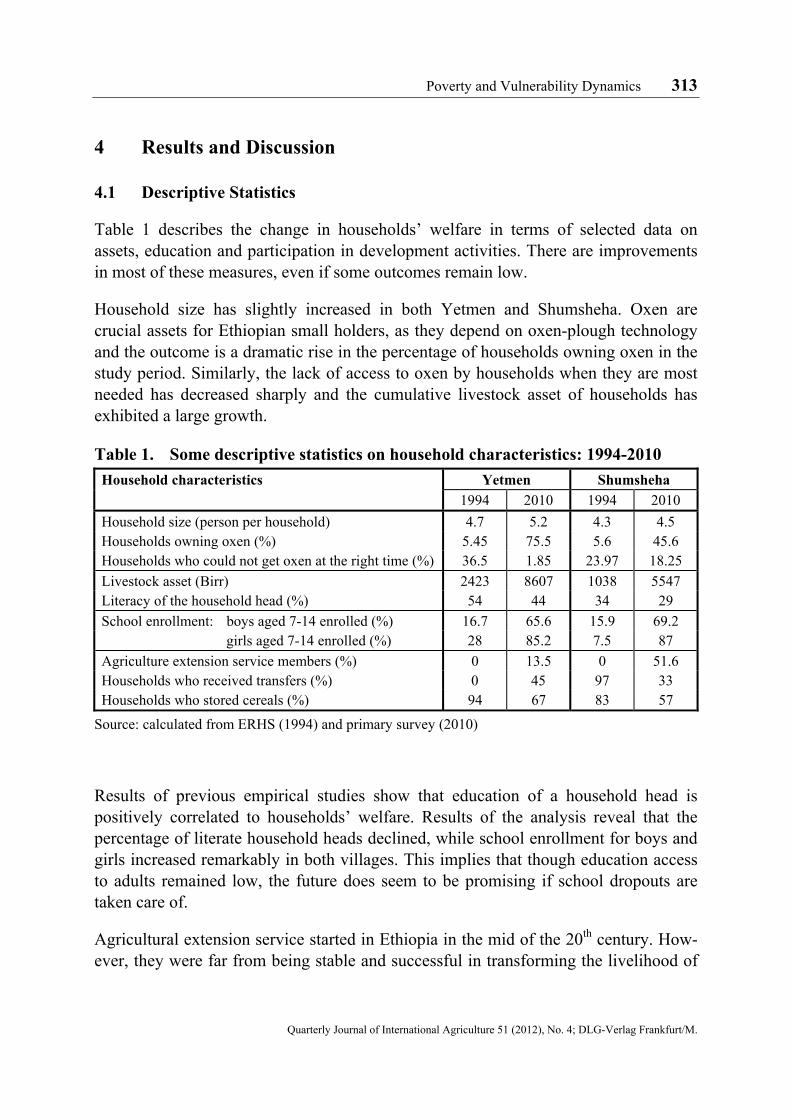
Table 1 describes the change in households’ welfare in terms of selected data on assets, education and participation in development activities. There are improvements in most of these measures, even if some outcomes remain low.

Household size has slightly increased in both Yetmen and Shumsheha. Oxen are crucial assets for Ethiopian small holders, as they depend on oxen-plough technology and the outcome is a dramatic rise in the percentage of households owning oxen in the study period. Similarly, the lack of access to oxen by households when they are most needed has decreased sharply and the cumulative livestock asset of households has exhibited a large growth.

Table 1. Some descriptive statistics on household characteristics: 1994-2010

Household characteristics Yetmen Shumsheha

1994 2010 1994 2010

Household size (person per household) 4.7 5.2 4.3 4.5 Households owning oxen (%) 5.45 75.5 5.6 45.6 Households who could not get oxen at the right time (%) 36.5 1.85 23.97 18.25

Livestock asset (Birr) 2423 8607 1038 5547 Literacy of the household head (%) 54 44 34 29

School enrollment: boys aged 7-14 enrolled (%) 16.7 65.6 15.9 69.2 girls aged 7-14 enrolled (%) 28 85.2 7.5 87

Agriculture extension service members (%) 0 13.5 0 51.6 Households who received transfers (%) 0 45 97 33 Households who stored cereals (%) 94 67 83 57

Source: calculated from ERHS (1994) and primary survey (2010)

Results of previous empirical studies show that education of a household head is positively correlated to households’ welfare. Results of the analysis reveal that the percentage of literate household heads declined, while school enrollment for boys and girls increased remarkably in both villages. This implies that though education access to adults remained low, the future does seem to be promising if school dropouts are taken care of.

Agricultural extension service started in Ethiopia in the mid of the 20th century. How-ever, they were far from being stable and successful in transforming the livelihood of



smallholders due to numerous impeding factors1. The incumbent government launched a new extension system in 1995 after a brief period of discontinuity since the fall of the Derg regime in 1991. This system was able to attract some farmers in both villages since then. However, its significance is more conspicuous in Shumsheha than Yetmen.

Results further indicate that households receiving transfers increased from nil to 45% in Yetmen compared to Shumsheha, which declined by two-third in 2010 from its level in year 1994. However, on average, Shumsheha has a predominant position compared to Yetmen. The main reason is that Shumsheha is one of the areas severely hit by the 1985 famine in Ethiopia and has been considered vulnerable village since then. As a result, it has been a beneficiary of safety net programs by the government and aid by other non-governmental organizations particularly in the aftermath of the famine to rehabilitate hard hit households. Finally, the percentage of households that store cereals has declined over the study period in both villages.

4.2 Changes in Relative Status of Welfare Groups

Previous poverty studies have been focusing most on the use of the standard classification of households into poor and non-poor. Instead of this practice, which focuses on a certain cut off point, a closer analysis on the behavior of the different consumption groups is immense importance and has become influential for policy analysis. Households were classified into different categories using real consumption expenditure per adult equivalent based on 1994 PPP prices. Accordingly, households in the sample are divided into five equal groups (quintiles) based on their real monthly consumption expenditure per adult equivalent values. The transition of households from their respective quintiles in 1994 to different consumption groups in 2010 is depicted in Table 2 below.

As depicted in Table 2, among those households in the third quintile (the middle 20%) in 1994, about 32% moved to lower quintiles (that is, 10% to the first quintile and 22% to the second quintile), 19% remained in the same quintile and the rest 49% moved to a higher quintile (23 and 26% to the fourth and fifth quintile respectively). Overall, in both PAs, 44.2% of households moved to a lower quintile, 16.8% remained in the same quintile and the remaining 39% moved to a relatively higher consumption groups. On the other hand, using transition matrices, as reported in Graph 1, the trend has been similar for the two villages over the panel period (1994-2010). The lion’s share is taken by households that moved to lower consumption groups followed by those who moved to upper quintiles and remained in the same groups respectively in

1 It would be advisable to read a paper by GEBREMEDHIN et al. (2006) on the evolution of extension

system in Ethiopia.



both villages. Overall, both PAs have exhibited higher mobility as shown by the Shorrock’s mobility index of 0.71 and 0.80 in Yetmen and Shumsheha respectively.

Table 2. Transition matrix for quintiles of real consumption expenditure between 1994 and 2010

2010 real monthly consumption expenditure per adult quintile (1 = lowest to 5 = highest; values are percentage of households)

1 2 3 4 5 Total

1994 real monthly consumption expenditure per adult equivlanet quintile

1 19 12 22 16 31 100 2 32 13 19 13 23 100 3 10 22 19 23 26 100 4 20 30 17 23 10 100 5 19 23 23 25 10 100

Total 100 100 100 100 100 100


Figure 1. Movement of households across quintile groups by PA (1994-2010)


4.3 The Foster-Greer-Thorbecke Indices

The Foster-Greer-Thorbecke (FGT) indices are the most widely used poverty indices that comprises of three measures: the incidence of poverty, also called the headcount index; the aggregate poverty gap (poverty depth); and the squared poverty gap (poverty severity). Poverty incidence refers to the percentage of people living below a minimum threshold as measured by local living standards. The poverty gap captures the mean aggregate consumption shortfall relative to the poverty line across the whole

0

20

40

60

80

100

Yetmen Shumsheha

%

PA

Same quintile position

Moved up

Moved down



population. In other words, it estimates the total resources needed to bring all the poor to the level of the poverty line. Poverty severity is a measure of relative deprivation among the poor, i.e., it takes into account not only the distance separating the poor from the minimum threshold but also the inequality among the poor. It places a higher weight on those households further away from the poverty line.

As aforementioned, an international poverty line of 1 USD per adult-day is used at purchasing power parity (about 1.92 Ethiopian Birr using 1994 base year prices according to World Bank, International Comparison Program Database)2. To make prices across PA and time comparable, the Food Price Indices (FPI) of Yetmen was used as a bench mark and deflated the FPI of Shumsheha for all years with an implicit assumption that food preferences of households remain the same across the panel rounds. Using this poverty line and the data on real monthly consumption expenditure per adult equivalent, the three FGT poverty indices have been computed for shumsheha and Yetmen for the four panel rounds.

Table 3. Foster-Greer-Thorbecke (FGT) indices and other descriptive statistics

FGT Indices PA 1994 1999 2004 2010

Head count index (%): Yetmen 32.07 46.30 15.38 32.00

Shumsheha 26.32 14.75 12.28 40.17

Poverty gap (%): Yetmen 3.80 5.08 1.60 2.09

Shumsheha 2.51 0.94 0.82 3.81

Squared poverty gap (%): Yetmen 1.11 0.80 0.21 0.22

Shumsheha 0.38 0.21 0.08 0.56

Mean monthly consumption expenditure per adult (Birr):

Yetmen 113.42 74.20 127.25 86.80

Shumsheha 116.69 129.74 159.58 124.13

Median monthly consumption expenditure per adult (Birr):

Yetmen 84.87 59.31 122.34 72.90

Shumsheha 79.60 99.41 111.86 66.39

Gini coefficient of inequality (%):

Yetmen 38.92 33.27 29.83 28.99

Shumsheha 42.17 34.62 39.39 55.07

Source: calculated from ERHS (1994, 1999 and 2004) and primary survey (2010)

The results indicate higher incidence of poverty, poverty gap and severity in Yetmen compared to Shumsheha in all the survey rounds except for the last round. This result is against our expectations as Shumsheha is considered as one of the most vulnerable

2 1 US dollar per adult/day is preferred in this article as poverty threshold since our estimation is

based on 1994 base prices. The exchange rate of 1 USD was 5 Ethiopian Birr (ETB) during the same year (DERCON and KRISHNAN, 1998).



PAs in Ethiopia in previous researches while Yetmen as a relatively better off PA in the northern highlands of Ethiopia (WEBB and VON BRAUN (1994) cited in DERCON and KRISHNAN (1998) and BEVAN and PANKHURST (1996)). This calls for an alternative approach of assessing poverty. Over the panel, Shumsheha has shown a consistent decline in poverty incidence until 2004 but a dramatic rise in 2010. The trend for Yetmen has been fluctuating throughout. Both mean and median real monthly consumption expenditures per adult equivalent fluctuated for Yetmen across the panel years. However, both measures have been consistently rising for Shumsheha in 1999 and 2004 before a substantial decline in the last round. When it comes to consumption expenditure inequality, higher inequality is observed throughout the panel years in Shumsheha compared to households in Yetmen as measured by the Gini-coefficient of inequality. The trend has a consistent decline for Yetmen but a considerable decline in Gini-coefficient in 1999 and a consistent rise afterwards for Shumsheha. In general, the uniform rise in all the poverty indices for both PAs over the last 5 years of the study could be partly associated with the rise in food prices in the country since 2006 and partly due to the collection of the 2010 data after six months of the 2009 harvest and appears to be supported by DERCON et al. (2011). They found a fall in median and mean consumption between 2004 and 2009 using the ERHS data for 15 villages in rural Ethiopia.

4.4 Decomposition of Poverty

In empirical work, decomposing inter-temporal poverty has been recognized as an important input for policies targeting on poverty. The respective policy responses for chronically poor section of the society differ from that of the transient one. Following the components approach, it was found that there is higher proportion of transient poverty in terms of headcount, poverty depth and severity as compared to the proportion of households under chronic poverty similarly in both PAs. Transient poverty is a dominant feature of the poor in both PAs. This implies that risk factors that push households into poverty have to be given due attention and concerted efforts must be directed to enhance the coping mechanisms of households to different kinds of shocks. To put it in a nutshell, adaptation and mitigation of risks should be emphasized.

Table 4. Poverty decomposition in Yetmen and Shumsheha (1994-2010)

Poverty type (percentages)

Head count (P0) Poverty gap (P1) Squared poverty gap (P2)

Yetmen Shumsheha Yetmen Shumsheha Yetmen Shumsheha

Chronic poor 0.122 0.051 0.021 0.009 0.001 0.002

Transient poor 0.189 0.197 0.069 0.057 0.038 0.024

Total poor 0.311 0.247 0.090 0.066 0.039 0.026

Chronic/total 0.608 0.798 0.767 0.864 0.974 0.923




On the other hand, Table 5 below provides good information about the movement of households over the panel years vis-à-vis to the poverty threshold, which is 1 USD per adult/day in 1999 PPP prices in this case. Based on FOSTER (2007), which considers households that are poor half or more of the times as chronic poor, it was found that dominant proportion of households in both PAs are under transient poverty followed by persistently poor in Yetmen and non-poor households in Shumsheha. Nearly 39% of households in Yetmen and over 45% in Shumsheha have been under transient poverty. The respective proportions of non-poor and chronic-poor households are 26.53% and 34.69% for Yetmen whereas 31.31% and 23.23% for Shumsheha.

Table 5. Poverty episodes 1994 to 2010 (based on 4 rounds)

Poverty status Yetmen (% of households)

Shumsheha (% of households)

Never poor 26.53 31.31

Poor once 38.78 45.45

Poor in 2 out of 4 rounds 22.45 18.18

Poor 3 out of 4 rounds 8.16 3.03

Poor in all rounds 4.08 2.02

Total 100.00 100.00


4.5 Asset-based Versus Consumption-based Poverty Estimates

PCA does not provide an easy way to generate a best-fit model to develop an index. The approach requires trial and error and continual scrutiny of variables to determine which combination yields the most logical results. The primary strategy is to systematically screen the list of variables that could be used in the model without compromising the explanatory power of the index. Despite the limitations of data, an attempt was made to accommodate different dimensions of poverty in the selection of variables based on a handful of literature in the area (such as FILMER and PRITCHETT, 1998; SAHN and STIFEL, 2000; BOOYSEN et al., 2005; and LIVERPOOL and NELSON, 2010). Accordingly, after successive trial and error, six variables were selected for developing the index based on their strong correlation with the poverty indicator benchmark, which is real monthly consumption expenditure per adult equivalent, and a compromise to capture different dimensions of poverty. The six factors are namely number of ploughs owned, number of oxen owned, number of adult labor, livestock asset (excluding oxen), size of cultivated land and number of crops grown for final formulation of the index for the sample households in both PAs.



The PCA has been conducted at household level. All the six factors finally selected to develop the asset-based poverty index have their factor coefficients well above 0.300 to be screened following Burt-Banks formula. The value of the Kaiser-Meyer-Olkin (KMO) measure of sampling adequacy is 0.73 indicating that the model is commendable.

The results of the PCA also indicate that the first factor explains 43.76% of the total variation in the data. The second factor explains only about 17.37% of the variance. The first component loading coefficients, which are the most critical outputs for determining the composition of the asset-based poverty index, are shown in the component matrix indicated in Table 6.

Table 6. Component matrix of the PCA analysis for the pooled data (1994-2010)

Factors at household level Mean Standard deviation

First component loadings

Size of cultivated land (ha) 1.411 0.948 0.595

Number of oxen owned per household 0.838 0.972 0.684

Number of ploughs owned 1.564 1.944 0.687

Number of adult labor per household 2.506 1.409 0.583

Value of livestock asset (Birr) 3,050.618 4,302.910 0.811

Number of crops cultivated 2.740 1.957 0.578

Source: own computation from ERHS (1994 and 2009)

The component matrix in Table 6 shows the loadings in the first component, which explains the highest variation in the data compared to the successive component loadings. All the factor coefficients have the expected sign consistent to previous literature. Besides, value of livestock asset, number of oxen owned and number of ploughs owned have the highest component loadings.

A correlation analysis was done for each year to examine the extent to which the index is associated with some of the factors commonly known to indicate poverty such as average real consumption expenditure per adult equivalent, mean value of food consumption per month, mean value of household assets owned, among others. The results show that the index is highly and significantly correlated with the variables in the expected directions. For example, the Pearson correlation with average real consumption expenditure per adult equivalent is 0.26, 0.27, 0.26 and 0.30 for the years 1994, 1999, 2004 and 2010 respectively with 1% significance in all cases, indicating the validity of our index in measuring the relative poverty status of smallholders in Northern Highlands of Ethiopia.



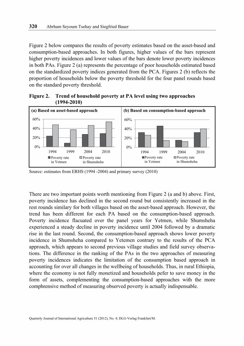
Figure 2 below compares the results of poverty estimates based on the asset-based and consumption-based approaches. In both figures, higher values of the bars represent higher poverty incidences and lower values of the bars denote lower poverty incidences in both PAs. Figure 2 (a) represents the percentage of poor households estimated based on the standardized poverty indices generated from the PCA. Figures 2 (b) reflects the proportion of households below the poverty threshold for the four panel rounds based on the standard poverty threshold.

Figure 2. Trend of household poverty at PA level using two approaches (1994-2010)

(a) Based on asset-based approach (b) Based on consumption-based approach

Source: estimates from ERHS (1994 -2004) and primary survey (2010)

There are two important points worth mentioning from Figure 2 (a and b) above. First, poverty incidence has declined in the second round but consistently increased in the rest rounds similary for both villages based on the asset-based approach. However, the trend has been different for each PA based on the consumption-based approach. Poverty incidence flacuated over the panel years for Yetmen, while Shumsheha experienced a steady decline in poverty incidence until 2004 followed by a dramatic rise in the last round. Second, the consumption-based approach shows lower poverty incidence in Shumsheha compared to Yetemen contrary to the results of the PCA approach, which appears to second previous village studies and field survey observa-tions. The difference in the ranking of the PAs in the two approaches of measuring poverty incidences indicates the limitation of the consumption based approach in accounting for over all changes in the wellbeing of households. Thus, in rural Ethiopia, where the economy is not fully monetized and households pefer to save money in the form of assets, complementing the consumption-based approaches with the more comphrensive method of measuring observed poverty is actually indispensable.

0%

20%

40%

60%

1994 1999 2004 2010

Yetmen ShumshehaPoverty rate in Yetmen

Poverty rate in Shumsheha

0%

20%

40%

60%

1994 1999 2004 2010Yetmen ShumshehaPoverty rate in Yetmen

Poverty rate in Shumsheha



4.6 Determinants of Poverty Dynamics

A thorough analysis of poverty requires a satisfactory study on the causes of poverty beyond a routine description of poverty profiles if we are able to tackle the root causes of poverty. Hence, this part of the paper attempts to address the question of what causes poverty. Both fixed effects IV and Multinomial Logit model (MLM) are employed for this purpose. The fixed effects model has been carried out using the log of real annual consumption expenditure per adult equivalent and PCA calibrated poverty indices as dependent variables for the consumption-based and asset-based approaches respectively covering the whole panel data. The Hausman’s specification test rejected the null hypothesis that coefficients of the regressors are not statistically different, which rules out the use of random effects model in both approaches. Again, the time dummy relevancy test was carried out and their use is supported in both cases. However, Hausman-Wu test revealed the presence of endogeneity problem in one of the regressors. Hence, the Fixed Effects Instrumental Variable (FEIV) regression model is applied. Size of cultivated land is found to be endogenous similarly in both the consumption and asset based regressions. The endogenous variables were predicted by regressing them against the exogenous variables in the system and used their predicted and lagged values as instruments. Hansen J test confirmed the validity of the instruments (see Appendix Table A).

Turning to the results, most of the important variables have similar association with the poverty indicator dependent variables in both models with the exception of transfers, which have been found to have different signs in the two models. In both regressions, size of cultivated land increases the welfare of households positively at 1% level of significance indicating that land is a crucial asset for mixed farming smallholders, which our data is taken from, in Ethiopia. Households headed by males appear to be associated with lower level of poverty only limited to the asset-based approach, which is significant at 1% level of significance. This reflects the low level of empowerment as well as entitlement of females to valuable assets (such as land) in rural Ethiopia in general and in our sample in particular.

Specific to the asset-based regression, household size is found to have a negative association, while household assets and engagement in off-farm activities correlate positively with welfare of households all at 10% level of significance. The former result is in line with previous studies in Ethiopia by RAMAKRISHNA and DEMEKE (2002) and in Kenya by Nyariki et al. (2002), which reported a negative association between household size and food security. On the other hand, the positive impact of household size on household income and food security has been found by ALENE and MANYONG (2006) in Nigeria and DEMEKE et al. (2011) in Ethiopia. However, the rationale behind these two opposing results lies on the demographic composition of households. In a household having more dependents, large household size would mean



more pressure on the income-generating members of the household and hence impacting on households’ poverty status. The latter two variables are as expected and as previous empirical results confirmed except the significance level is low in this case. On the other hand, the significance of credit and number of plots (a proxy for land fragmentation) are limited to the consumption based approach. Whilst credit is positively associated with welfare of households, land fragmentation has a negative and significant correlation.

Table 7. FEIV regression for analyzing the determinants of poverty for the whole sample

Variables FEIV (Asset based) FEIV (cons based)

Coefficient (SE) Coefficient (SE)

Sex of household head (dummy: 1 for male) 0.32654 (0.09020)*** 0.17108 (0.13413)

Age of household head 0.01885(0.01450) -0.04555 (0.02851)

Age square of household head -0.00020 (0.00015) 0.00041 (0.00028)

Literacy of the household head (dummy: 1 Yes)

0.09945 (0.12164) -0.03920 (0.12942)

Household size -0.23434 (0.13769)* -0.00570 (0.04188)

Size of cultivated land (ha) 0.36401 (0.07119)*** 0.49135 (0.13413)***

If transfers received (dummy: Yes 1; No 0) -0.24963 (0.11203)** 0.23499 (0.12049)*

Saving’s group (dummy: 1 for member) 0.01236 (0.07009) 0.16922 (0.13475)

Credit (dummy: 1 for member) 0.47377 (0.43242) 0.18498 (0.11093)*

Monetary value of livestock (Birr) 0.00010 (0.00002)*** 0.00001 (0.00001)

Engagement in off-farm activities (dummy: Yes 1; No 0)

0.00015 (0.00008)* -0.00001 (0.00017)

Extension service 0.02918 (0.07298) 0.16676 (0.12868)

Number of crops grown (proxy for crop diversification)

0.13505 (0.01541)*** 0.05483 (0.02953)*

Number of plots of land (proxy for land fragmentation)

0.04285 (0.02662) -0.08774 (0.05101)*

Household assets (Birr) 0.00003 (0.00002)* 0.00001(0.00005)

Time dummy (base: 1999)

Year 1999 1.85808 (0.31660)*** 1.67800 (0.53481)***

Year 2004 0.41710 (0.16816)** 0.63921(0.11559)***

Constant -1.42116 (0.36754)*** 4.429745 (0.67827)***

F(14, N) 26.26 7.37

Prob > F 0.000 0.0000

N 273 286

Robust standard errors in parentheses *** p<0.01, ** p<0.05, * p<0.1




Though transfers have significant values in both models, the coefficients have different signs. Households receiving transfers are negatively associated with higher levels of poverty incidence at 5% level of significance in the asset-based approach while positively correlated in the consumption-based approach with only 10% level of signi-ficance. Previous empirical results assert the association of transfers in either ways as explained in section 3 of this paper. However, the result of the asset-based approach appears to be strong and more plausible as previous studies show that the impact of transfers on welfare tend to be negative particularly in the long term (in our case, 4 rounds in 16 years). On the other hand, in both approaches number of crops grown (a proxy for crop diversification) is found to have a significant and positive association with the dependent variable as expected.

Credit access significantly contributes to improvement of households’ welfare limited to the asset-based regression while engagement in off-farm activities is positively correlated to the dependent variable in the consumption-based regression at 10% level of significance. Though formal financial institutions and micro-enterprises are scant in rural Ethiopia in general and in the sampled peasant associations in particular, the positive role played by social linkages and local savings and credit associations could be visible in the study areas.

Due to the use of lagged instruments, 1994 is dropped and 2010 is used as a base year and the time dummies show a significant improvement in the average welfare of households in 2004 and 1999 respectively in both models. Finally, most of the empirical results reported here correspond to the outcomes of the foregoing descriptive statistics.

In addition to the Fixed Effects IV model, the Multinomial Logit (MNL) model is estimated. The MNL uses a categorical variable of being chronically poor, transient poor and non-poor (base category) as a dependent variable to be regressed against the different household characteristics of the base year (1994 in this case) and a village dummy variable. Results are shown in Table 8 below. MNL is based on a strong assumption of Independence of Irrelevant Alternatives (IIA). Hence, we employed the Hausman IIA test, which indicates that the assumption is not violated, which makes the use of MNL to be appropriate. The explanatory variables included in the model are jointly significant at 1% and the McFadden’s pseudo R2 value associated with the models is 0.2, which indicates that the fitness of the model is pretty satisfactory.

Based on results, households headed by male are less likely to remain in a state of chronic and transient poverty in the region with 10 and 1% level of significance, respectively. This is in line with the less empowerment of women as well as their limited access to assets in Ethiopia especially in rural areas. This supports the results of the asset-based regression shown in Table 7. Households headed by relatively younger adults are negatively associated with transient poverty, while those headed by



older adults have positive association with transient poverty with 10% level of significance in both cases. Land fragmentation is positively associated with transient poverty at 5% level of significance. This supports the regression result of the asset-based approach shown in Table 7. Moreover, the larger the household size the higher is the probability of households being trapped in persistence poverty as compared to the non-poor households with 5% level of significance. The implication of this result is that most members of the households are inactive and are dependent on the productive adult members and hence increasing the risk of households falling into poverty. Households with larger household assets are likely to be in chronic poverty, which is significant at 10% level. Both of the above-mentioned results further support the robustness of the asset-based approach compared to the consumption-based method.

Table 8. MNL model for analyzing the determinants of poverty for the whole sample

Variables Transient poverty Chronic poverty

Coefficient (SE) Coefficient (SE)

Sex of household head (dummy: 1 for male) -2.69876 (0.95712)*** -1.93450(1.05745)*

Age of household head -0.25974 (0.14324)* -0.12792 (0.15842)

Age square of household head 0.00251 (0.00148)* 0.00135 (0.00160)

Literacy of the household head (dummy: 1 Yes) 0.54398 (0.61177) 0.31785 (0.68098)

Household size 0.20620 (0.20252) 0.54898 (0.21964)**

Cultivated land (ha) -0.04990 (0.33322) -0.51849 (0.40218)

If transfers received (dummy: 1 Yes; 0 No) 0.70239 (1.97328) -0.03884 (1.89321)

Saving’s group (dummy: 1 for member) -1.49396 (0.99619) -0.00801 (0.88769)

Credit (dummy: 1 for member) -0.74032 (0.55385) -0.62977 (0.61116)

Monetary value of livestock (Birr) -0.00008 (0.00018) 0.00002 (0.00017)

Engagement in off-farm activities (dummy: Yes 1; No 0)

0.00038 (0.00043) -0.00103 (0.00240)

Number of crops grown (proxy for crop diversification)

-0.23392 (0.20630) -0.20155 (0.236547)

Number of plots of land (proxy for land fragmentation)

0.41115 (0.19213)** 0.46876 (0.21237)

Household assets (Birr) -0.00153 (0.0010) -0.00360 (.00199)*

Village dummy ( 1 if Yetmen, 0 otherwise) 1.32713 (2.11246) 1.08215 (2.07464)

Constant 6.74751 (3.71044)* 1.82930 (4.03025)**

F(14, N) 47.39

Prob > F 0.0023

N 120

Robust standard errors in parentheses *** p<0.01, ** p<0.05, * p<0.1




4.7 Vulnerability to Poverty

Vulnerability has long been ignored as valuable and necessary component to poverty in poverty literature. It has gained momentum in recent times as a result of its crucial contribution to policy making. Besides, even though poverty assessment studies have been immensely used for policy purposes, they have been providing only an ex-post measure of households’ wellbeing (or lack thereof) as an input for poverty reduction strategies. As such, they do not provide a tool for apriori prevention of poverty incidences as a result of unforeseen risks. Hence, vulnerability studies complement poverty studies by providing an ex-ante measure of wellbeing.

Previous studies attach closely related but different definitions to vulnerability to poverty. In this paper, the working definition of vulnerability to poverty refers to the risk of an individual or a household to fall below the poverty line or, for those already below the poverty line, to remain in or to fall further into poverty.3 The paper uses 0.5 as a vulnerability threshold. The results of the three steps FGLS model are reported in Table 9.

Figure 3. Vulnerability to poverty for both peasant associations (1994-2010) Yetmen Shumsheha

Source: estimates from ERHS (1994-2004) and primary survey (2010)

According to the consumption-based approach, the proportion of households observed to be poor and vulnerable to poverty followed similar trends over the panel years in both PAs. However, the comparison has been different between the two PAs. Households in Shumsheha have exhibited a consistent decline in both poverty incidence and vulnerability to poverty measures except for a sharp rise in 2010, 3 Adopted from JHA et al. (2009)

0

10

20

30

40

50

60

1994 1999 2004 2010

%

Year

0

10

20

30

40

50

60

1994 1999 2004 2010

%

Year

Poverty Incidence - StandardVulnerability to PovertyPoverty Incidence - PCA



whereas those in Yetmen witnessed fluctuations in both measures. On the other hand, according to the asset-based approach, the trends of poverty incidence for both PAs are similar as already mentioned in Figure 2. It is, however, pretty visible from Figure 3 that the levels of poverty incidences have been consistently higher in Shumsheha than Yetmen across the panel years.

Apart from an assessment of the trends of vulnerability to poverty in the two PAs, it is important to investigate the causes behind the difference in vulnerability of households to poverty between the two PAs over the four survey rounds. In this regard, fixed effects instrumental variable model was estimated after carrying out Hausman’s specification test and Hausman-Wu endogeneity test. Results of the Hasuman-Wu test indicate that equb, transfers and number of crops are endogenous variables in Yetmen, whereas participation in off-farm activities is the sole endogenous regessor for Shumsheha. Following the same procedure used in identifying the determinants of poverty, endogenous variables were predicted by regressing them against the exogenous variables in the system. Then, the predicted and lagged values were used as instruments. Hansen J statistic confirmed the validity of the instruments (see Appendix Table B).

Table 9. Covariates of vulnerability to poverty using fixed effects IV approach

Vulnerability Index FEIV – Yetmen (1994-2010)

FEIV – Shumsheha (1994-2010)

Sex of the household head -0.01105 (0.06769) 0.06418 (0.06834)

Age of the household head -0.03924 (0.01648)** 0.04931 (0.01291)***

Age squared of the household head 0.00045 (0.00019) -0.00047 (0.00012)***

Household size 0.04636 (0.01734)*** 0.05408 (0.02121)***

Literacy of head (dummy: Yes=1) -0.02331 (0.07753) 0.07546 (0.09573)

Credit (dummy: Yes=1) -0.24341 (0.08748)*** -0.19408 (0.05934)***

Membership in local savings group (dummy) 0.19735 (0.1426448) -0.01432 (0.06275)

Proportion of fertile land (%) -0.00183 (0.00087)** 0.00011 (0.00091)

Number of oxen owned 0.00236 (0.05507) -0.06353 (0.03731)*

Number of ploughs owned -0.00793 (0.01724) 0.00222 (0.00849)

Number contacts with extension agents -0.01635 (0.01302) 0.01294 (0.01374)

Engagement off-farm activities (dummy) -0.00004 (0.00007) -0.00038 (0.00017)**

Number of crops grown in the year -0.01876 (0.02470) -0.07960 (0.01579)***

Number of plots -0.00645 (0.02232) -0.00359 (0.01864)

If transfers received (dummy: Yes 1; No 0) 0.49582 (0.36101) -0.16112 (0.04179)***

If households stored cereals (dummy: Yes 1; No 0) -0.24290 (0.08093)*** -0.04924 (0.05435)

Lag of vulnerability to poverty index 0.05124 (0.07742) 0.01476 (0.03666)

Constant 0.84043 (0.42310)** -0.88735 (0.36594)**

F(17, N) 8.51 15.79

Prob > F 0.0000 0.0000

Source: calculated from ERHS (1994-2004) and primary survey (2010)



The result shows that the causes of vulnerability to poverty have indeed been different in the two PAs. All the significant variables have the expected signs and support the foregoing results on the determinants of poverty except for the age and age squared of the household heads in Shumesheha. Against apriori expectations, households headed by younger individuals are associated with higher vulnerability, while their counterparts (embodied in age-squared variable) are less likely to be vulnerable to poverty for households in Shumsheha. These results appear to reflect the often ignored reality in this part of the country that younger adults (usually new couples in the context of rural Ethiopian) face challenges of having limited command on vital resources of farming such as land, oxen and other social assets, which increases their likelihood of falling into poverty. On the other hand, besides the small size of households headed by the aged, due to the presence of strong bond among extended families in rural Ethiopia, parents receive all rounded and unreserved cooperation from the families of their independent children that could positively affect the welfare of households with aged household heads. In both villages, whilst household size tends to increase vulnerability to poverty, access to credit appears to lessen vulnerability of households to poverty at 1% level of significance in both cases. Young household heads, proportion of fertile land and households that store cereals are significantly less vulnerable to poverty than their counterparts in Yetmen. On the other hand, number of oxen owned, number of crops grown, participation in off-farm activities and receiving transfers reduce the likelihood of households falling into poverty trap at least for one more year significant only to households in Shumsheha.

5 Concluding Remarks

In this paper, an attempt is made to analyze poverty dynamics using consumption-based approaches (components and spell approaches) and asset-based approach (PCA). Using Fixed Effects IV and Multinomial Logit models, the determining factors of poverty have been investigated. On the other hand, vulnerability to poverty and its determinants are examined using three step Feasible Generalized Least Square and Fixed Effects IV models, respectively.

Despite the substantial improvements in most of the measures of households’ welfare (in terms of selected data on assets, education and participation in development activities) over the study period, households moving to lower quintile consumption groups have dominated the sample. Considerable number of the households in both villages has been poor and vulnerable to poverty using 1 USD and 0.5 as poverty and vulnerability threshold respectively. However, a consistent decline in both measures has been observed in Shumsha until 2004 but increased dramatically in 2010 while the trend has been fluctuating for Yetmen over the entire panel years.



Decomposition of poverty into chronic and transient components using the components approach (FGT) revealed that transient poverty is dominant in the study area compared to that of chronic poor. This result was also supported by the Spells approach following the method by FOSTER (2007) indicating that programs targeting poverty should primarily focus on risk factors that swing households in and out of poverty such as drought, conflict, price fluctuations and the like. This essentially requires enhancing smallholders’ access to insurance schemes; provision of credit facilities; promoting off-farm activities and helping farmers use improved technologies such as drought resistant seed varieties, irrigation facilities and so on.

A comparison of the consumption-based poverty measures with that of the asset-based approach provides two interesting results. First, despite the difference in the trends of poverty incidence experienced by the PAs in the two poverty measurement approaches, both measurements offer similar results in that poverty incidence has been on the rise in each of the PAs in the last survey round. Second, the consumption-based approach shows lower poverty incidence in Shumsheha compared to Yetmen contrary to the results of the PCA approach, which is supported by previous village studies. The difference in the ranking of the PAs in the two approaches of measuring poverty incidences indicates the limitation of the consumption-based approach in accounting for over all changes in the wellbeing of households. Thus, complementing the con-sumption-based approach with the more comphrensive method of measuring observed poverty is indispensable.

Results of the asset-based approach appear to be more robust than the consumption-based approach in terms of the fitness of the model as well as based on the results of third alternative approach: the multinomial logit model. Accordingly, land, livestock asset, crop diversification and male headed households are found to be associated with lower poverty levels while household size and transfers to higher poverty levels. One of the key policy variables for smallholders in Ethiopia, i.e. agricultural extension service, is found to have no meaningful relationship with smallholders’ welfare in both villages indicating the need for the evaluation of the service in this part of the country in addition to strengthening incentives and monitoring mechanisms so that this decisive policy tool might serve the target it is intended for.

Smallholders’ access to saving, credit and off-farm activities is very limited in rural Ethiopia. Except few local (informal) credit and savings institutions and self created off-farm activities, formal institutions for such services are almost non-existent. The insignificance of these variables in many of the foregoing regression results reveals this reality. Hence, increasing smallholders’ access to such services in required by supporting local savings and credit institutions as well as making them to be pro-poor is vital. As traditional savings and credit institutions tend to include the poorest, they



need to be supported to accommodate a wider range of services, including insurance, that enable poor households to invest in and protect their assets, particularly from higher incidence events (such as common health risks) and covariate shocks (such as extreme weathers) since transient poverty is pervasive in the sample.

Moreover, awareness creation on family planning, enhancing smallholders’ participation in off-farm activities, increasing their crop diversification, making targeted and timely transfers, encouraging farmers to store cereals, and improving their storage facilities would significantly reduce vulnerability of households to poverty in the region. Not all the important variables for poverty reduction work for reducing vulnerability of house-holds to poverty or do they impact similarly. Therefore, for a meaningful intervention, strategies aimed at reducing poverty should critically consider factors that make households vulnerable to poverty in a particular context. Finally, a piecemeal approach to solving individual problems is by no means sufficient to overall poverty alleviations. A comprehensive package of strategies that creates good governance, helps establish functional infrastructure, build schools and heath centers, and foster innovations and technologies is needed to lift rural households out of poverty trap and sustain pro-poor growth.

References ALENE, A. and M. MANYONG (2006): Endogenous Technology adoption and household food

security: the Case of Improved Cowpea Varieties in Northern Nigeria. In: Quarterly Journal of International Agriculture 45 (3): 211-230.

BENTLEY, J. (1987): Economic and Ecological Approaches to Land Fragmentation: In Defence of a Much-Aligned Phenomenon. In: Annual Review of Anthropology 16 (1987): 31-67.

BEVAN, P. and A. PANKHURST (1996): Report on the Sociological Dimension of the Ethiopian Rural Economies Project. Mimeo. Center for the Study of African Economies, Oxford, UK.

BIGSTEN, A. and A. SHIMELES (2008): The Persistence of Urban Poverty in Ethiopia: A Tale of Two Measurements. Working Papers in Economics No 283. Göteborg University, School of Bussiness, Economics and Law.

BOOYSEN, F., S. BERG, R. VAN DER, R. BURGER, M. von Maltitz and G.Du. Rand (2005): Using an Asset Index to Assess Trends in Poverty in Seven Sub-Saharan African Countries. Presented at the The Many Dimensions of Poverty, Brasilia, Brazil. The International Poverty Centre of the United Nations Development Programme (UNDP), Brasilia.

BRANDOLINI, A., S. MAGRI and T.M. SMEEDING (2009): Asset-Related Measures of Poverty and Economic Stress. Presented at the Measuring Poverty, Income Inequality, and Social Exclusion: Lessons from Europe. Organization for Economic Cooperation and Development, Paris.



– (2010): Asset-based Measurement of Poverty. In: Journal of Policy Analysis and Management 755 (29): 267-284.

CAVATASSI, R., B. DAVIS and L. LIPPER (2004): Estimating Poverty Over Time and Space: Construction of A Time Variant Poverty Index for Costa Rica. ESA Working Paper No. 04-2.1. Agricultural and Development Economics Division, The Food and Agriculture Organization of the United Nations (FAO), Rome.

CHAUDHURI, S., J. JALAN and A. SURYAHADI (2002): Assessing household Vulnerability to Poverty from Cross-Sectional Data: A Methodology and Estimates from Indonesia. Discussion Paper No: 0102-52. Columbia University, New York, USA.

DEMEKE, A., A. KEIL and M. ZELLER (2011): Weather Risk, Social Capital and Household Wellbeing in an Agrarian Economy: Empirical Studies on Ethiopian Smallholders (Vol. 123). Magraf Publishers GmbH, Weikersheim, Germany.

DERCON, S., J. HODDINOTT and T. WOLDEHANNA (2011): Growth and Chronic Poverty: Evidence from Rural Communities in Ethiopia. CSAE Working Paper, WPS/2011-18. Department of Economics, University of Oxford, UK.

DERCON, S. and P. KRISHNAN (1998): Changes in Poverty in Rural Ethiopia 1989-1995: Measurement, Robustness Tests and Decomposition. Discussion Paper Series DPS 98.19. Center for Economic Studies, Katholieke Universiteit, Leuven, Belgium.

FILMER, D. and L. PRITCHETT (1998): Estimating Wealth Effects Without Expenditure Data - or Tears: An Application to Educational Enrollments in States of India. World Bank Policy Research Working Paper No. 1994. World Bank, Washington, DC.

FOSTER, J.E. (2007): A Class of Chronic Poverty Measures. Working Paper No. 07-W01. Department of Economics, Vanderbilt University, Nashville, USA.

GEBREMEDHIN, B., D. HOEKSTRA and A. TEGEGNE (2006): Commercialization of Ethiopian Agriculture; Extension Service from Input Supplier to Knowledge Broker and Facilitator. ILRI, Nairobi, Kenya.

GLEWWE, P. and G. HALL (1995): Are Some Groups More Vulnerable to Macroeconomic Shocks than others? Hypothesis Tests Based on Panel Data from Peru. In: Journal of Development Economics 56 (1998): 181-206.

GROOTAERT, C. and R. KANBUR (1995): Child Labor: A Review. Background Paper for World Development Report. Policy Research Working Paper 1454. World Bank, Washington, DC, USA.

HAGOS, F. and S. HOLDEN (2003): Rural Household Poverty Dynamics in Northern Ethiopia 1997-2000: Analysis of Determinants of Poverty. Presented at the Chronic Poverty Reseaach Center International Conference, Manchester, UK.

ISLAM, N. and A. SHIMELES (2007): Poverty Dynamics in Ethiopia: State Dependence and Transitory Shocks. Working Papers in Economics No. 260. School of Business, Economics and Law, Göteborg University.

JALAN, J. and M. RAVALLION (2000): Is Transient Poverty Different? Evidence from Rural China. In: Journal of Development Studies 36 (6): 82-100.

JHA, R., T. DANG and K. SHARMA (2009): Vulnerability to Poverty in Fiji. In: International Journal of Applied Econometrics and Quantitative Studies 6 (1).



KANBUR, R., M. KEEN and M. TUOMALA (1994): Labour Supply and Targeting in Poverty Alleviation Programs. The International Bank for Reconstruction and Development/THE WORLD BANK. In: World Bank Economics Review 8 (2): 191-211.

KEDIR, A.M. and A. MCKAY (2003): Chronic Poverty in Urban Ethiopia: Panel Data Evidence. Presented at the Staying Poor: Chronic Poverty and Development Policy, Institute for Development Policy and Managment, University of Manchester, UK.

LIVERPOOL, L.S.O. and A.W. NELSON (2010): Assets Versus Consumption Poverty and Poverty Dynamics in the presence of Multiple Equilibria in Rural Ethiopia. IFPRI Discussion Paper 00971. Development Strategy and Governance Division, International Food Policy Research Institute (IFPRI).

MANGIAVACCHI, L. and P. VERME (2011): Cash Transfers and Household Welfare in Albania: A Non-experimental Evaluation Accounting for Time-Invariant Unobservables. The World Bank, Washington, DC.

MCCULLOCH, N. and B. BAULCH (2002): Simulating the Impact of Policy Up On Chronic and Transitory Poverty in Rural Pakistan. Institute of Development Studies, University of Sussex, Brighton.

NYARIKI, M., L. WIGGINS and K. IMUNGI (2002): Levels and Causes of Household Food and Nutritional Insecurity in Dry Land Kenya. In: Ecology of Food and Nutrition 41 (2): 155-176.

ODURU, G., E. AGGGREY, G. BANNI, A. CROPPENSTEDT and Y. AGYAPONG (2003): Explaining Success in Reducing Under-Nourishment Numbers in Ghana. ESA Working Paper No. 03-10. FAO, Rome, Italy.

QUARTEY, P. (2006): The Impact of Migrant Remittances on Household Welfare in Ghana. AERC Research Paper 158. African Economic Research Consortium, Nairobi, Kenya.

RAMAKRISHNA, G. and A. DEMEKE (2002): An Empirical Analysis of Food Security in Ethiopia: the Case of North Wello. In: Africa Development XXVII (1 and 2): 127-143.

RODGERS, J.R. and J.L. RODGERS (1993): Chronic Poverty in the United States. In: Journal of Human Resources 28 (1): 25-54.

SAHN, D.E. and D.C. STIFEL (2000): Poverty Comparisons Overt Time and Across Countries in Africa. In: World Development 28 (12): 2123-2155.

SUNDQVIST, P. and L. ANDERSSON (2006): A Stud of the Impacts of Land Fragmentation on Agricultural Productivity in Northern Vietnam. Uppsala University, Department of Economics.

TOULMIN, C. (1986): Access to Food, Dry Season Strategies and Household Size Amongst the Bambara of Central Mali. In: International Development Studies Bulletin 17 (3): 58-66.

WOOLDRIDGE, J. (2002): Econometric Analysis of Cross Section and Panel Data. MIT Press, Boston, USA.

WORLD BANK (2001): World Development Report 2000/2001: Attacking Poverty: Opportunity, Empowerment and Security. Washington, DC.



– (2012): Country Reports on Health, Nutrition, Population and Poverty. URL: http://www.worldbank.org/poverty/health/data/intro.htm, retrieved June 13, 2012.

Acknowledgment

The first author would like to thank Deutscher Akademischer Austausch Dienst (DAAD) for funding the research. I am also most grateful for the Department of Economics (AAU), IFPRI and CSAE (University of Oxford) for allowing me access the ERHS data.

Contact author: Abrham Seyoum Tsehay Justus-Liebig-University, Senckenbergstr. 3, 35390 Gießen, Germany e-mail: [email protected]

Appendix

Table A. Hansen J tests of over identification for the fixed effects IV regressions

Sample Chi-square P-value Asset-based regression 0.135 0.7137 Consumption based regression 0.001 0.9701

Note: The null hypothesis is that instruments are not correlated with error terms. The null is accepted in all equations and that all instruments in the respective equations are found to be valid.


Table B. Hansen J tests of over identification for the fixed effects IV regressions

Sample Chi-square P-value Yetmen 6.266 0.0993 Shumsheha 1.399 0.4967

Note: The null hypothesis is that instruments are not correlated with error terms. The null is accepted in all equations and that all instruments in the respective equations are found to be valid.


poverty and vulnerability dynamics: empirical - agecon search

Documents