Population Densities of Poison Dart Frogs in a Regenerating Tropical Forest

as Measured by the Hayne Estimator

A Thesis Presented

by

Jennifer Rose Bunnell Miller

To the Joint Science Department

Of The Claremont Colleges

In partial fulfillment of

The degree of Bachelor of Arts

Senior Thesis in Organismal Biology

April 2007

TABLE OF CONTENTS

ABSTRACT................................................................................................................................. 4

INTRODUCTION ......................................................................................................................... 5

MATERIALS AND METHODS ................................................................................................... 14

Study Area ........................................................................................................................... 14

Study Species....................................................................................................................... 17

Population Density.............................................................................................................. 19

Distribution ......................................................................................................................... 22

Abiotic Factors.................................................................................................................... 22

RESULTS ................................................................................................................................. 25

Population Densities and Distributions.............................................................................. 25

Rainfall................................................................................................................................ 32

Temperature ........................................................................................................................ 33

Time of day.......................................................................................................................... 34

DISCUSSION............................................................................................................................. 37

Hayne Estimator Validity.................................................................................................... 37

Population Densities and Distributions.............................................................................. 41

Temperature ........................................................................................................................ 44

Time of Day......................................................................................................................... 45

The Hayne Estimator as a Tool for Monitoring Amphibians ............................................. 46

Conclusions......................................................................................................................... 47

ACKNOWLEDGEMENTS........................................................................................................... 49

LITERATURE CITED................................................................................................................ 50

2

APPENDICES............................................................................................................................ 56

3

ABSTRACT

With amphibian populations declining throughout the world, there is an increasing

demand for effective tools to measure species responses to environmental change. This study

investigates the effectiveness of the Hayne Estimator in evaluating the densities of two

species of poison dart frogs in three Costa Rican lowland forest habitats with varying degrees

of recovery from deforestation (selectively-logged riparian forest, post-pasture secondary

forest and non-native bamboo plantation forest). Population densities of Dendrobates

granuliferus and Dendrobates auratus were significantly highest in riparian forest,

substantially lower in bamboo, and very low in secondary forest. This trend corresponds to

previous research on species recolonization after deforestation and subsequent regrowth and

indicates that the Hayne Estimator is well suited for the evaluation of poison dart frogs.

Abiotic factors such as proximity to water, rainfall, temperature and time of day were found

to have some effect on frog sighting frequency. Individuals of both species tended to

aggregate near water, but the proportional distribution of transects according to all habitat

water presence likely negated this effect. Rainfall was unrelated to the sighting frequency of

D. auratus but correlated with the sighting frequency of D. granuliferus. Air temperature did

not impact sighting frequency. Time of day, however, was found to influence the sighting

frequencies of both species, with peaks occurring in the early morning and late afternoon.

The robustness of the Hayne Estimator when used to monitor poison dart frogs suggests that

the technique may be a valuable tool for future conservation research.

4

INTRODUCTION

Since scientists gathered at the First World Congress of Herpetology in 1989 to

address the worldwide decline of amphibian populations, concern for these creatures has

increased at an accelerating rate (Phillips, 1990; Stuart et al., 2004). Now, nearly 2 decades

later, as populations continue to decrease in size and weaken in stability, scientists are calling

for the unprecedented cooperation of all to prevent further loss of amphibian diversity. In

2006, 49 accomplished herpetologists co-authored a forum in Science that announced the

disappearance of 122 species and identified 32.5% of known amphibians as threatened

(Mendelson III et al.). The group asserted that only through the union of “individuals,

governments, foundations, and the wider conservation community” would the escalating rate

of extinctions slow. Their recommendations echo the suggestions of other scientists and

necessitate the implementation of monitoring, surveys, habitat protection and breeding

research colonies in an international effort to ensure the continued existence of amphibians.

Long-term monitoring programs serve as a foundation of restoration ecology planning

because they reflect the responses of at-risk species to environmental change. Knowledge

about the population health of sensitive species in recovering habitats is invaluable to the

conservation community. These studies not only increase the likelihood of successful land

management of protected areas, but they also guide policy towards accurately prioritizing the

protection of land in regions and habitats that are greatly valued for preserving biodiversity.

Without a doubt, Latin America has been more severely impacted by amphibian

declines than any other region in the world (International Union for Conservation of Nature

and Natural Resources [IUCN], 2006). In Central and South America, over 30 genera, 9

families and 1,157 species of amphibians have declined or gone extinct (Young et al., 2001;

5

6

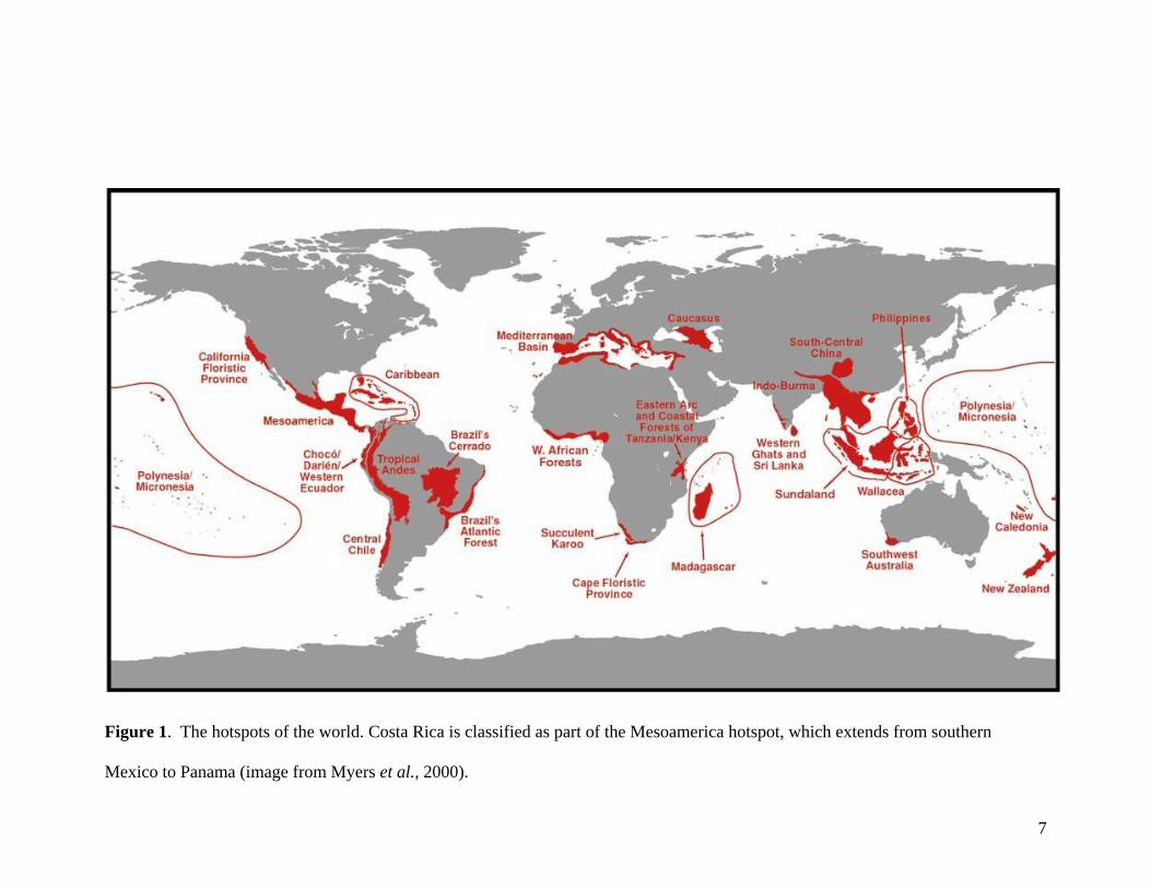
IUCN, 2006; Pounds et al., 2006). The tropical regions of this area have supported a high

diversity of amphibian species for millennia, leading the region to be classified as a

biodiversity hotspot (Figure 1; Myers et al., 2000; Brooks et al., 2002). When one considers

the increasing rate of new amphibian species discoveries (Donoghue and Alverson, 2000),

the potential number of amphibians that may have been harmed by human activities is

astounding.

Because of the extensive body of tropical ecological research conducted in Costa

Rica, this country has become a paradigm for understanding patterns of species decline in

other tropical locations. Although Costa Rica covers only 0.03% of the planet’s surface, it is

home to 4% of the world’s biodiversity and 3% of the world’s threatened amphibians (IUCN,

2006; World Resources Institute, 2006; National Biodiversity Institute, 2007). To date, one

amphibian species has gone extinct in the country (Bufo periglenes, the golden toad) and 64

species are considered threatened (IUCN, 2006). Although more than one-fifth of Costa

Rican land is protected, it is clear that further action must be taken in order to raise, or at

least sustain, the current level of biodiversity (World Resources Institute, 2006).

Like many other countries throughout the world, Costa Rica has been the site of

rampant deforestation over the past few centuries. However, human habitation has followed a

unique trend within the last several decades. With increasing job opportunities in the urban-

based tourism and textile industries, workers have begun to migrate away from agricultural

areas (Aide and Grau, 2004). Since 1960, the rural population in Latin America and the

Caribbean has dropped by 30%, a trend driven in part by a 20 million person decrease in the

population whose livelihood is based on agriculture, hunting, fishing or

7

Figure 1. The hotspots of the world. Costa Rica is classified as part of the Mesoamerica hotspot, which extends from southern

Mexico to Panama (image from Myers et al., 2000).

forestry since 1980 (Food and Agriculture Organization of the United Nations, 2004). While

much of the vacant land has been sold for the expansion of other farms, a substantial amount

has been abandoned, providing an opportunity for regrowth, recolonization and the

reestablishment of natural ecosystems.

While ecologists have extensively explored species’ responses to the degradation of

native habitat, less work has been done on recovering habitats. With the current trend in

Costa Rica favoring natural regrowth, and with the increasing public awareness about the

causes of global warming, a large movement to restore farmed and developed land across the

planet could occur within the next century. Species monitoring programs must be

implemented in order to predict, prepare and assist the associated changes in biodiversity.

In 2001, Pitzer College acquired the Firestone Center, a parcel of land in Costa Rica

that had previously been selectively stripped of forest and converted into a cattle farm and

Figure 2. The Firestone

Reserve, otherwise known as

the Finca la Isla del Cielo, is

owned by Pitzer College and

located near Dominical in

southwestern Costa Rica

(Firestone Center for

Restoration Ecology, 2006).

8

monoculture plantation (Figure 2). A series of changes in ownership has allowed the

Firestone Reserve to have 13 years of continuous natural regeneration. Today, the preserve is

an ideal study site for investigating the process of regrowth. The variation in land patch

quality permits the juxtaposition of species in native riparian habitat versus secondary and

non-native plantations that have had over a decade to recover. The Joint Science Department

of the Claremont Colleges launched a student research program in the summer of 2005 and

has plans to establish long-term monitoring programs to track the regeneration progress.

Since it is unrealistic to study the impacts of human activities on all species in a given

area, indicator species are studied as representatives of a larger group. Indicators may belong

to any taxonomic group, but are commonly characterized by a degree of sensitivity to

disturbance that mirrors the responses of a wide variety of other species (Landres et al.,

1988). Anurans are ideal indicators because all stages of their life cycles are highly

dependent on environmental conditions. Most frogs and toads require a permanent water

source for reproduction, the development of young, and a source of food. Their skins are

permeable to permit survival in water and on land, leaving their bodies vulnerable to the

chemical balance around them. The majority of anurans also consume insects, a group known

to shift radically with a change in vegetation (Gibbs and Stanton, 2001). Based on these

characteristics and others, anurans are especially susceptible to habitat loss, chemical

contamination, climate change and the introduction of exotic species and disease, factors

known as the leading causes of decline in other amphibian species as well (Young et al.,

2001).

Although anurans are prized for the insight they provide regarding the health of an

ecosystem, the creatures are also the arch nemeses of many field scientists. Cryptic and

9

nocturnal, the typical frog or toad is a challenge to study in its natural environment. The

endemic poison dart frogs of Costa Rica, however, provide a colorful alternative to studying

cryptic indicators in the tropics. All members of the family Dendrobatidae are

aposematically colored, diurnally active and easily identified to species. Seventeen species of

Dendrobates have been identified in Central America and more than 100 species are known

to South America (Maxson and Myers, 1985). In addition to the two-continent family

distribution, many poison dart frog species have a range that spans several countries. Data

collected on frogs in one region can thus be readily applied to an entirely different area.

In an effort to measure the biodiversity status in the regenerating Firestone Reserve

habitats, the abundances of two poison dart frog species were measured. Both the granular

Error!

Figure 3. Many frogs utilize camouflage to hide from predators and field scientists alike

(left, Hyla versicolor), whereas Dendrobatids have conspicuous skin color and patterns to

contrast against their background (right, Dendrobates azureus). Their aposematic coloration

conveys to predators the consequences of a quick snack. Photos courtesy of

www.livingunderworld.org and www.webshots.com

10

Figure 4. The study species: Dendrobates granuliferus (top) and Dendrobates auratus

(bottom). Photographs by Keith Christenson.

11

(Dendrobates granuliferus) and the green and black (Dendrobate auratus) poison dart frog

occur naturally on the preserve (Figure 4). The population densities of these species were

assessed in riparian, secondary and bamboo forest habitats during the early wet season of

October 2006. Data were collected and calculated using the Hayne Estimator technique

(Hayne, 1949), which utilizes measurements taken from observations of sighting angle and

distance to each animal. The densities were then applied to approximate frog recolonization

in the secondary and bamboo habitats as compared to the more pristine riparian habitat.

Because the method assumes that an individual will flush and be readily noticeable as

the observer approaches, the Hayne Estimator is not well designed for the cryptic, nocturnal

habits of most amphibians but has been repeatedly employed to evaluate populations of birds

and mammals (Coulson and Raines, 1985; Pelletier and Krebs, 1997). The conspicuous

coloration and diurnal activity periods of Dendrobatid frogs makes them potentially

appropriate for the Hayne Estimator technique. This study explores the utility of poison dart

frogs as subjects for the Hayne Estimator while investigating the quality of vegetation

regrowth at the Firestone Reserve as a means of supporting native levels of biodiversity.

To account for the impact of abiotic factors on frog sighting frequencies, proximity to

water, as well as correlations with rainfall, air temperature and time of day, were considered.

Because past studies indicate that poison dart frogs do not depend on large bodies of water

(reviewed by Savage, 1968; Vences et al., 2000; Jowers and Downie, 2005), random

distribution was expected. Rainfall and time of day have both been identified as influential

factors, with some Dendrobatids occurring in larger quantities in the presence of rain and in

the early morning and late afternoon (Graves, 1999). Finally, the air temperature was not

12

anticipated to affect sighting frequencies because of its small range due to the tropical

climate.

13

MATERIALS AND METHODS

Study Area

Field research was conducted at the Firestone Center for Restoration Ecology with the

permission of Pitzer College and the Joint Science Department. Claremont Colleges. The

Firestone Reserve is a 60 ha protected preserve of lowland (15m – 303 m) Pacific Moist

Forest in southwestern Costa Rica near Dominical (16.684 N, 51.643 W). The reserve has a

unique history that makes the area a suitable research site for an examination of poison dart

frog populations in regenerating habitats. Beginning around 1950, the property was

completed deforested, with the exception of two precipitous stream canyons within which

circa 100 m wide strips of riparian forest were only selectively logged (Firestone Center for

Restoration Ecology, 2006). The land was utilized as a cattle farm until 1993, when the

property was purchased by Ms. Firestone and converted into a combined sustainable farm

and private biological preserve. At this time, livestock were removed and parts of the land

were replanted with monoculture crops, including 5.9 ha of bamboo (Guadua aculeata, G.

angustifolia, Dendrocalamus asper, and D. latiflorus), 1 ha of bananas (Musa acuminata), 1

ha of black palm (Bactris gasipaes), and 24.7 ha of mixed hardwood tree species.1 The

remaining 27.4 ha were allowed to regenerate naturally. In 2005, the property was donated to

Pitzer College and farming maintenance was abandoned. The land has since been left alone

to regrow and is currently used as a biological reserve for education and research by the

Pitzer Study Abroad Program and the Claremont Colleges Joint Science Department.

The division of the reserve into multiple sub-habitats makes it an ideal location for

the study of biodiversity in recovering natural and non-native vegetation. The Firestone

1 Refer to http://costarica.jsd.claremont.edu/biodiversity/trees.shtml for an up-to-date listing of identified species.

14

15

Reserve borders the Hacienda Baru National Wildlife Refuge to form a contiguous 390 ha

sanctuary dedicated to scientific study and eco-tourism with minimal biological impact

(Hacienda Baru National Wildlife Refuge, accessed 2006).

This study focuses on Dendrobatid presence in three types of habitat on the Firestone

Reserve: selectively-logged riparian forest (from hereon referred to as “riparian”), abandoned

pasture (“secondary”) and bamboo plantation (“bamboo”; see Figure 5). The riparian regions

consist of primary forest with tall vegetation and dense canopy cover. The ground in this

habitat is shaded during most of the day and was usually covered by thick leaf litter. No

records are available that describe the method of selective logging in this habitat, leaving no

way to judge whether the land is an accurate standard of natural vegetation. However, the

riparian habitat of the Firestone Reserve is visually indistinguishable from the primary forest

of the Hacienda Baru National Wildlife Refuge. Therefore, the riparian habitat was used in

this study as a representative of natural forest conditions, although it should be recognized

that there are potential influences of the past selective logging that are unmeasured in this

study.

The secondary forest is comprised of lower, thinner trees than the riparian habitat.

Large patches of sunlight are often observed on the ground, causing grasses to replace damp

leaf litter throughout much of the secondary forest (Figure 5). The bamboo habitat features

thick groves of tall culms that provide moderate amounts of shade. Sunlight filters through

the vegetation at a lower intensity than in the secondary forest, and dense, knee-high

vegetation covers the ground around the bamboo. Multiple sources of water exist in all three

sampling habitats. Small and moderate, 1-10 m wide streams run through both the riparian

and secondary forests, while three large ponds border the bamboo habitat.

16

Figure 5. A map of the Firestone Reserve habitats with images of the three habitats of study: bamboo (top left), riparian forest (bottom left) and secondary forest (top right). The

six transects are numbered and differentiated by color. Prominent water sources are represented by light blue symbols (filled polygon = pond; solid line = stream, known location;

dotted line = stream, estimated location [surveyed by McFarlane, 2001 {unpubl. data}]). Photographs by author.

Observations were systematically made within each habitat by following the pre-

established trails of the reserve as transects for observation. The use of four maintained trails

permitted an accessible and repeatable loop through the forest and covered all three types of

habitat. The trails were divided into six transects of varying lengths, with most transects

covering multiple habitats (Table 1). The order that transects were walked was randomized

when possible so as not to cause unintentional correlations with time. Transects 1 and 4 could

not be shuffled because they provided starting and ending access or connected path loops,

respectively.

Table 1. Length distributions for study transects.

Habitat length (m) Transect

Trail ID*

Total length (m) Riparian Secondary Bamboo

1 WT 275.9 275.9 0 0 2 B 949.9 84.1 865.8 0 3 C 838.6 721.3 117.3 0 4 B 646.2 194.5 451.7 0 5 BB 985.6 0 236.6 749.0 6 C 100.5 100.5 0 0

*Trail ID corresponding to the survey by McFarlane, 2001 (unpubl. data).

Study Species

The combined Firestone-Hacienda Baru area hosts at least 28 known species of

anurans (M. Ryan, pers. comm.), including Dendrobates granuliferus, the granular poison

dart frog, and D. auratus, the green and black poison dart frog. While both species are

abundant on the Firestone Reserve, D. granuliferus is internationally recognized as a

threatened species due to habitat loss and degradation as well as human harvesting of the

species (IUCN, 2006). The range of D. granuliferus is also limited, covering 5,579 km2 from

17

the mid-western coastal lowlands of Costa Rica to the northern border of Panama (Global

Amphibian Assessment, 2006; IUCN, 2006). Dendrobates auratus is considered to be of

lesser concern, largely because of its greater range of 11,944 km2 from northern Costa Rica

through northern Columbia and higher tolerance of habitat degradation.

Dendrobates granuliferus and D. auratus were selected as study subjects because of

their relevance to amphibian declines and their conspicuous appearances in the field.

Dendrobatids have many natural history characteristics typical of tropical amphibians. All

species are diurnal and commonly live among the low vegetation and leaf litter of moist

forests below elevations of 3,000 m (Savage, 1968). They are considered terrestrial anurans

because their life cycles are independent of large water sources. Dendrobatid eggs are laid on

land and tadpoles are carried on the backs of their parents to temporary puddles of water

among vegetation. Dendrobatids specialize in eating ants but also consume a large quantity

of mites, insects that are also characteristic of the diets of other tropical amphibians such as

Atelopus, Bufo and Bolitoglossus (Toft, 1981; Anderson and Mathis, 1999). They mate

during the wet season like many other tropical amphibians, and they are most active between

May and November (reviewed by Savage, 2002). Because many of the human impacts that

threaten D. granuliferus and D. auratus also affect other tropical amphibians and potentially

other groups of organisms, these two species serve well as indicators of the status of tropical

wildlife populations.

In addition, these species were chosen because their unique aposematic coloration

makes them convenient to study in the field. While many anuran species are nocturnal and

camouflaged to their environments, Dendrobatids are diurnal and have brilliantly colored

skin markings. The coloration serves as a signal to predators, warning them of the toxic

18

alkaloids that can be released from the frogs’ skin glands as a mechanism of defense

(Saporito et al., 2004). The distinctive patterns of D. granuliferus and D. auratus permit easy

sighting of individuals and allowed for a high confidence in the accuracy of the field

techniques used in this study.

Frogs were observed on the Firestone Reserve during the wet season between 6

October and 14 October 2006. The research period corresponded to the Dendrobatid mating

season and the peak of their activity throughout the year (reviewed by Savage, 2002).

Observing at this time guaranteed the highest number of frog sightings possible, leading to

elevated estimates of population densities and an overall optimistic perspective of the

Dendrobatid presence on the Firestone Reserve.

Population Density

The population density of frogs was measured with the Hayne Estimator (Hayne,

1949). To keep measurement technique consistent, all observations were made by the author.

Two sessions of observations typically occurred each day. The first session began at

approximately 7:00 and ended around 11:00 and the second began at approximately 13:30

and ended around 16:30. Transects were walked at a constant speed from start to stop without

pause, except to record frog measurements. Consequentially, transects with many frog

sightings took longer to walk than transects with few sightings.

Each observation followed the same protocol. When a frog was sighted, the observer

immediately took three measurements (Figure 6):

(1) The distance from the observer to the frog’s location at first sighting. Measurements

were made using a Leica Geosytems laser rangefinder accurate to ± 3mm and later

19

trigonomically corrected from incline distances (i.e. from the height of the hand-held

rangefinder) to true plan distances.

(2) The magnetic bearings of the transect and frog, using a Suunto sighting compass

readable to ± 0.5 degrees.

(3) The time of the sighting.

Occasionally, when a frog was observed well beyond the first possible point of contact, the

observer back-tracked her steps until she reached the location where the frog first came into

view. For example, if a frog was first noticed when the observer was directly beside it, the

observer retraced her steps until she could first view the frog amidst the vegetation.

Obscurities due to vegetation occasionally caused sighting difficulties, but errors were most

likely not frequent enough to largely impact data. This technique corrected for the limitation

Figure 6. A visual representation of the

Hayne Estimator data collection

technique, showing the distance from the

observer to the frog (ri) and the

corresponding measured sighting area

(shaded red).

20

of being able to view only one side of a transect at a time.

The location of each frog was recorded relative to a surveyed map of the reserve

paths. A survey of current habitat borders was mapped during the study period and overlaid

on the original path survey. Survey information was used to relate frog sighting to habitat

type for use in the Hayne Estimator. Total transect length and average segment (i.e. the

distance between transect turns) length were also collected from the survey.

The population densities of D. granuliferus and D. aruatus for each observation

session were calculated for each habitat using the unmodified Hayne Estimator:

Dh =n

2L1n

1rii= t

n

∑⎛

⎝ ⎜

⎞

⎠ ⎟ ,

where Dh is the Hayne density estimate, n is the number of animals observed, L is the

transect length, and ri is the sighting distance to the ith animal. The standard deviation was

calculated by taking the square root of the variance, calculated as:

Variance(DH ) ≈ DH2 var(n)

n2 +

1r,

− R⎛

⎝ ⎜

⎞

⎠ ⎟

2

i= t

n

∑R2n n −1( )

⎡

⎣

⎢ ⎢ ⎢ ⎢ ⎢

⎤

⎦

⎥ ⎥ ⎥ , ⎥ ⎥

where R is the mean of the reciprocal of the sighting distances and calculated as:

R =1n

1rii= t

n

∑ ,

Circular statistics on sighting angles were computed using the StatistiXL Excel Add-

In (http://www.statistixl.com/). Population densities were analyzed with VassarStats (Lowry,

2007) for statistical differences between the species and habitats using One-Way Independent

ANOVA and Tukey HSD tests.

21

Distribution

To relate frog sightings to actual geographical features, ArcGIS Version 9.1 was used

to project the Firestone trail survey into a satellite image of the Firestone Reserve (obtained

from Digital Globe, Inc.) with reference to GPS coordinates collected at the site. Habitat

zones were constructed using several older habitat maps of the reserve as well as records of

current habitat boundaries taken during the study. Frog sighting points were imported and

displayed with graduated symbols to represent point densities. Water sources (streams and

ponds) were approximated and drawn by hand according to the trail survey (McFarlane,

2001, unpubl. data) and satellite image.

The proximity of each sighting to water was determined using COMPASS software

(Version 5.05; Fish, 2005) The straight-line distance between each sighting location and the

closest water source was measured and then correlated to the number of frogs sighted at the

location using a linear regression calculated with VassarStats (Lowry, 2007).

Abiotic Factors

To determine whether the transect distribution proportionally represented the amount

of water in each habitat, an analysis of transect-resource proportionality was conducted using

measurements from the Firestone maps created with ArcGIS to compare the ratio of the

habitat area within 50 m of a water source to the total habitat area versus the transect length

(by habitat) to the total transect length (by habitat). In other words,

area of habitat within 50m of watertotal area of habitat

: tran sec t length in habitat within 50m of watertotal length of tran sec t in habitat

22

Rainfall and air temperature (from now on referred to as “reserve temperature”) were

measured every 2 hours by a Davis Weatherlink meteorological station on the Firestone

Reserve. Average reserve temperature was calculated for each increment as the arithmetic

mean of the high and low temperatures. To test for a correlation between reserve temperature

and the frog sighting frequency, data were analyzed using a linear regression calculated with

Vassar Stats (Lowry, 2007). VassarStats was also used to determine whether a correlation

existed between rainfall and frog sighting frequency with a Pearson’s chi-square 2x2

contingency table test. To evaluate overall trends in frog sighting frequency, data from both

species were combined and compared to the time of sighting.

The air temperature in each habitat (from now on referred to as “habitat temperature”)

was measured using four temperature loggers (Stow Away XTI). One logger was attached to

a tree in each habitat and the sensor was oriented to hang freely (Figure 7). The loggers were

positioned so that they received light levels typical of the particular habitat (i.e. not in full

sunlight). A fourth control logger was set in a deforested meadow on the reserve to measure

the highest possible daily temperature (i.e. full sunlight). Loggers were set to record data for

each day and night of the study period and measured the habitat temperature every 5 or 20

minutes, depending on the format available on the logger. Temperature data from all the days

in the study period were averaged to find the 24-hour mean temperature fluctuation for each

habitat. The fluctuations of all habitats were then compared to determine whether a large

difference in temperature in any of the habitats may have influenced poison dart frog activity

levels.

23

Figure 7. Locations of the temperature loggers in each habitat: bamboo (left top), secondary

(bottom left), riparian (top right) and exposed meadow (bottom right). Photographs by

author.

24

RESULTS

Inconsistencies in data collected at the start of the study period have led to the

exclusion of several days of data from the final analysis. The number of frog sightings in the

first three days was significantly lower than sightings during the remainder of the observation

days (an average of 6 ± 6 observed frogs/km in contrast with 85 ± 39 observed frogs/km).

Additionally, no significant differences were found in abiotic factors such as rainfall or

temperature between the first 3 days and the subsequent days of observation. The lack of

disparity suggests that the initial low number of sightings was likely a result of the observer’s

learning period. A test run was not conducted ahead of time, leading the observer to learn the

sighting and measurement techniques during the official study period. Therefore, only data

from 9 October through 14 October 2006 were included in the analysis (Appendix A). Data

collected from 6 October to 8 October are listed in Appendix B but are not considered valid

data or incorporated into the thesis.

Population Densities and Distributions

A total of 166 D. granuliferus and 109 D. auratus were observed, resulting in a total

sample size of 275 frogs. The average population densities for both species were larger in the

riparian forest than in the secondary or bamboo habitats (Figure 8). For D. granuliferus, the

riparian density was estimated to be 68 times greater than the secondary density and 23 times

greater than the bamboo density. The D. auratus riparian density estimate was 155 times

greater than the secondary density but only three times greater than the bamboo density.

Bamboo densities were larger than secondary densities for both species, with density for D.

granuliferus in bamboo reaching an estimate that was three times larger than for secondary

25

forest and the density for D. auratus in bamboo estimated to be 47 times larger than in

secondary forest. ANOVA analysis indicated significant effects of habitats on densities for

both D. granuliferus and D. auratus (F = 20.31, df = 2, P < 0.0001; F = 28.62, df = 2, P <

0.0001, respectively).

0

0.2

0.4

0.6

0.8

1

1.2

1.4

1.6

1.8

2

2.2

Riparian Secondary Bamboo

Habitat Type

Den

sit

y (

fro

gs/

ha)

Figure 8. Average population densities of D. granuliferus (solid) and D. auratus (open) by

habitat. Vertical lines represent one standard deviation.

26

Population density trends differed through habitats between the two poison dart frog

species. The presence of D. granuliferus was nearly twice that of D. auratus in the riparian

forest, while the density of the D. auratus was more than four times larger than in the

bamboo. The population densities of both species in the secondary forest were very low,

although results indicated that D. granuliferus was sighted more often than D. auratus.

Tukey HSD tests found densities of riparian versus secondary habitats and riparian versus

bamboo habitats to be significantly different, but secondary versus bamboo habitats to be not

significant (P < 0.01, P < 0.01, P > 0.5, respectively).

A clear correlation between the number of frog sightings and proximity to water was

apparent for both species (Figure 9). Analysis with a linear regression indicated a significant

negative relationship between the number of sightings and the distances of the sighting

locations to a water source (y = -0.0476x + 13.478, df = 1, r2 = 0.207, P < 0.01). Three

particularly dense clusters of frog sightings are apparent in the riparian and secondary

habitats near streams, while sightings in the bamboo habitat did not appear to be correlated to

water (Figure 10).

The distributions of D. granuliferus and D. auratus were generally very similar.

Individuals of both species were found simultaneously at the same locations on multiple

occasions. Only two locations throughout the study site indicated the dominating presence of

one species without the other (Figure 11). For one, there is a distinct difference in the number

of D. auratus (n = 8) found in bamboo compared to D. granuliferus (n = 2). However, the

small sample size undermines the strength of this disparity. A second conspicuous

dissimilarity in distribution occurred on the southernmost stream where the trail dips towards

the southern stream.

27

Figure 9. A scatterplot showing the negative relationship between the number of sightings

(D. granuliferus and D. auratus combined) and the distance of the sighting location to a

water source in all three habitats. A linear trend line has been fit to the dat

y = -0.0476x + 13.478r2 = 0.2072

20

25

30

35

200 250 300

)

of

sigh

tin

g

0

5

10

15

0 50 100 150

Distance to water source (m

Nu

mber

s

28

Figure 10. Distribution of all frog sightings through the habitats of the reserve (D. granuliferus and D. auratus combined). Where multiple frogs were seen in the same location,

sighting frequencies are symbolized by graduated circles (see legend). Prominent water sources are represented by blue symbols (filled polygon = pond; solid line = stream, known

location; dotted line = stream, estimated location [surveyed by McFarlane, 2001 {unpubl. data}]).

29

Figure 11a. Distribution of Dendrobates granuliferus sightings through the habitats of the reserve. Where multiple frogs were seen in the same location, sighting frequencies are

symbolized by graduated circles (see legend). Prominent water sources are represented by light blue symbols (filled polygon = pond; solid line = stream, known location; dotted

line = stream, estimated location [surveyed by McFarlane, 2001 {unpubl. data}]).

30

31

Figure 11b. Distribution of Dendrobates auratus sightings through the habitats of the reserve. Where multiple frogs were seen in the same location, sighting frequencies are

symbolized by graduated circles (see legend). Prominent water sources are represented by light blue symbols (filled polygon = pond; solid line = stream, known location; dotted

line = stream, estimated location [surveyed by McFarlane, 2001 {unpubl. data}]).

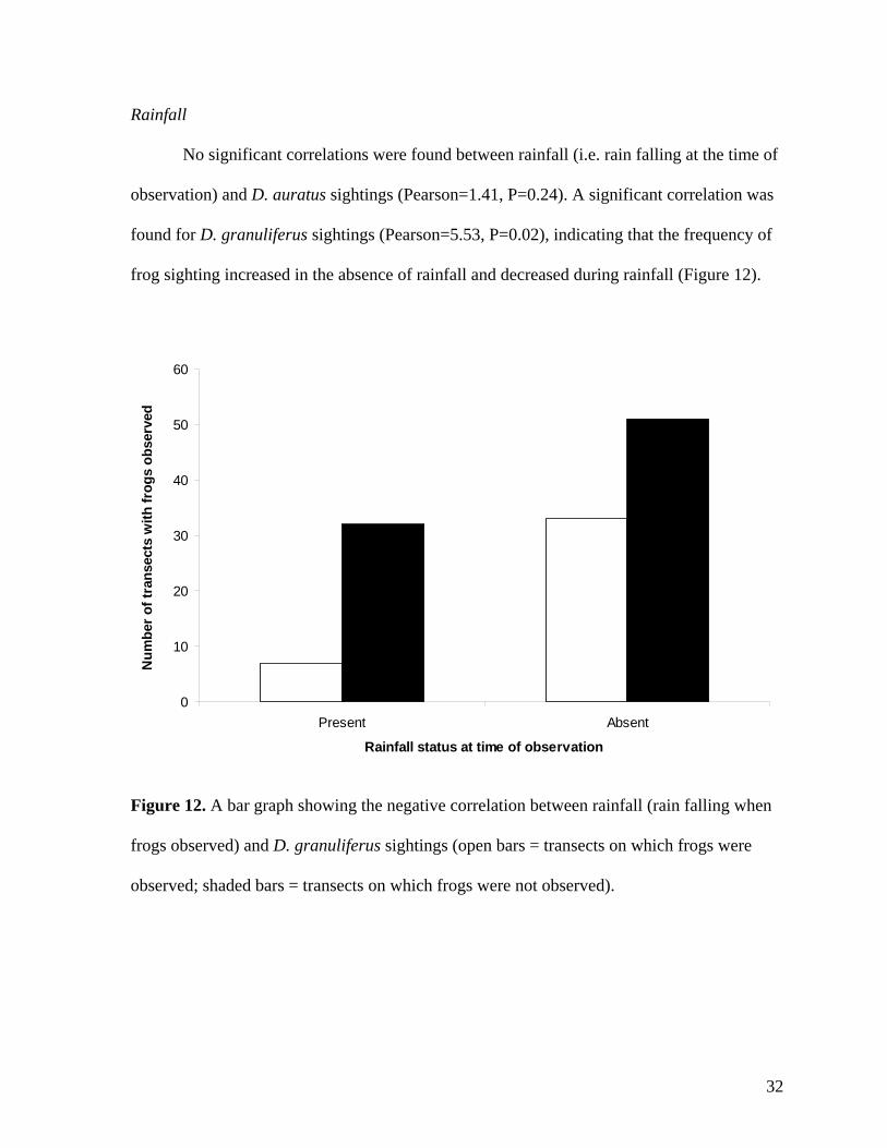
Rainfall

No significant correlations were found between rainfall (i.e. rain falling at the time of

observation) and D. auratus sightings (Pearson=1.41, P=0.24). A significant correlation was

found for D. granuliferus sightings (Pearson=5.53, P=0.02), indicating that the frequency of

frog sighting increased in the absence of rainfall and decreased during rainfall (Figure 12).

0

10

20

30

40

50

60

Present Absent

Rainfall status at time of observation

Num

ber o

f tra

nsec

ts w

ith fr

ogs

obse

rved

Figure 12. A bar graph showing the negative correlation between rainfall (rain falling when

frogs observed) and D. granuliferus sightings (open bars = transects on which frogs were

observed; shaded bars = transects on which frogs were not observed).

32

Temperature

Regression analyses found no significant relationship between temperature and frog

sightings for either D. granuliferus or D. auratus (y = -0.0031x + 0.0962, df = 17, P > 0.05,

r2 = 0.1378; y = -0.0012x + 0.0434, df = 17, P > 0.05, r2 = 0.0587, respectively). Temperature

varied only 7ºC according to the Firestone meteorological station during the time of

observation and ranged from 23ºC and 30ºC.

No large temperature differences were found between the riparian, secondary and

bamboo habitats. The temperatures of the study habitats consistently remained within 1˚ of

each other (Figure 13). In contrast, temperatures recorded in the deforested meadow

remained higher than in the study habitats, peaking at 6.6˚C higher than in the other habitats.

The temperature loggers indicated that the temperature in the three study habitats ranged

from 22.5˚C to 28˚C while the temperature in the deforested meadow ranged from 23.5˚C to

34.0˚C.

33

20

22

24

26

28

30

32

34

36

0:00

2:00

4:00

6:00

8:00

10:0

0

12:0

0

14:0

0

16:0

0

18:0

0

20:0

0

22:0

0

Time

Avera

ge a

ir t

em

pera

ture

(˚

C)

BambooSecondaryRiparianDeforested meadow

Figure 13. Mean daily temperature fluctuations in each study habitat and control

environment (deforested meadow).

Time of day

To evaluate overall trends in frog sighting frequency, data from both species were

combined and compared to the time of sighting (Figure 14). A large increase in the sighting

frequency was observed in the early morning (7:00 to 8:00), followed by relatively constant

rates in the later morning and early afternoon (8:00 to 12:00 and 13:00 to 14:00; no data was

collected from 12:00 to 13:00). From 14:00 to 15:00, a sharp decrease in sighting frequency

34

occurred, followed by a substantial increase in the late afternoon (16:00 to 17:00) and a sharp

decrease in the mid afternoon (14:00 to 15:00).

Data separated by species show less extreme patterns of change over time. Sighting

frequency of D. granuliferus peaked in the early morning (7:00 to 8:00) and rose again in the

later morning (10:00 to 11:00) and mid afternoon (15:00 to 17:00), but remained

approximately constant at all other times of the day (Figure 15). Dendrobates auratus

sighting frequency also peaked in the early morning (7:00 to 8:00) but remained relatively

constant throughout the rest the day, with low dips in activity in the mid morning (10:00 to

11:00) and mid afternoon (14:00 to 15:00).

0

0.02

0.04

0.06

0.08

0.1

0.12

0.14

0.16

7:00 8:00 9:00 10:00 11:00 13:00 14:00 15:00 16:00

Time

Fro

g s

igh

tin

g f

req

uen

cy (

fro

gs/

m)

Figure 14. Total frog sighting frequency over time (D. granuliferus and D. auratus

combined). Vertical lines indicate one standard deviation.

35

Gran/m vs. Time

0

0.01

0.02

0.03

0.04

0.05

0.06

0.07

0.08

0.09

7:00 8:00 9:00 10:00 11:00 13:00 14:00 15:00 16:00

Time

Fro

g

sig

hti

ng

fre

qu

en

cy (

fro

gs/

m)

0

0.01

0.02

0.03

0.04

0.05

0.06

0.07

0.08

0.09

7:00 8:00 9:00 10:00 11:00 13:00 14:00 15:00 16:00

Time

Fro

g s

igh

tin

g f

req

uen

cy (

fro

gs/

m)

Figure 15. Sighting frequency of D. granuliferus (top) and D. auratus (bottom) over time.

Vertical lines indicate one standard deviation.

36

DISCUSSION

Hayne Estimator Validity

The Hayne Estimator makes several assumptions that were met to the fullest extent

possible (Hayne, 1949):

(i) Animals are distributed randomly and independently throughout the area of

study.

(ii) Animals on the transect line are observed with a probability of one.

(iii) Sightings are independent events.

(iv) Animals are motionless until stimulated to flush by the observer.

(v) Each animal has a specific circle of detection in which the animal will flush

when stimulated by the observer’s presence.

(vi) The mean sighting angle between the observer’s path and the animal is 32.7˚.

(vii) Animals are not counted more than once.

(viii) Distances are measured without error.

(ix) Sighting conditions remain consistent during the study.

Assumption i challenges the instinctive nature of wild animals to cluster near

beneficial resources and when mating. Since breeding pairs of D. granuliferus and D. auratus

only come into contact for a short period during courting and amplexus (Dunn, 1941;

Summers et al., 1999), mating was not believed to substantially impact overall frog

distribution during the study. Additionally, because most organisms prefer to have easy

access to water, food, shelter and other similar necessities, animals disperse non-randomly.

However, the quantity of a given resource in a study site can be proportionally represented by

the amount of transect length that includes the particular resource. Both D. granuliferus and

37

D. auratus tended to be sighted more often when closer to a water source (Figure 9); in fact,

50% of frogs were observed within 50 m of a water source. An analysis of transect-resource

proportionality was conducted using measurements from the Firestone maps created with

ArcGIS to compare the ratio of the habitat area within 50 m of a water source to the total

habitat area versus the transect length (by habitat) to the total transect length (by habitat). In

other words,

area of habitat within 50m of watertotal area of habitat

: tran sec t length in habitat within 50m of watertotal length of tran sec t in habitat

Riparian habitat yielded a habitat : transect water ratio of 1.00, secondary habitat yielded a

ratio of 0.70 and bamboo habitat yielded a ratio of 0.88 (Table 2). Generally, the transects in

all three habitats were found to be distributed proportionally and represented the amount of

water in each habitat, therefore accurately reflecting a proportional number of frog sightings

between the habitats. The lower ratio of the secondary habitat is an indicator that this habitat

contained fewer water sources than the others and may be a primary cause of the low number

of frog sightings (n = 2). The high ratios in all habitats suggests that the distribution of the

transects throughout the study site upheld assumption i of the Hayne Estimator.

Table 2. Analysis results of the transect-resource proportionality test.

Habitat type Proportion of habitat area within 50 m of

water

Proportion of transect length within 50 m of

water

Ratio of habitat to transect proportions

Riparian 0.71 0.70 1.00 Secondary 0.15 0.21 0.70 Bamboo 0.23 0.26 0.88

38

The consistency of sighting method maintained assumption ii. Because this project

was carried out in a tropical rainforest, the density of vegetation was unpredictable and

variable in different areas of the transects. Consequentially, the probability of sighting a frog

declined quickly as one moved farther away from the center of the trail. However, brush did

not tend to obstruct the transect itself and frogs sitting directly on the path were visually and,

often, audibly conspicuous.

Sightings were treated as independent events (iii) by counting each frog as an

individual observation, even if frogs were within close proximity to each other. However, the

study was conducted during the wet season, when poison dart frogs mate (Savage, 2002).

The aggregating of frogs may have altered the normal distribution of frogs throughout the

study site, but the effect of mating on the data has not been explored.

Assumptions iv and v are well suited for the study of poison dart frogs. When

approached, both D. granuliferus and D. auratus typically remained motionless or hopped

slowly until the observer was within about 3 m. At this point, the frog increased its rate of

movement until hidden by vegetation or at a location determined safe by the frog.

Occasionally frogs remained stationary despite the close proximity of the observer;

measurements in these cases were taken from the first possible sighting location as

determined by the observer. The density of vegetation may have had some impact on the

observer’s ability to see frogs, e.g. the bamboo habitat had less vegetation within 2 m of the

ground than the riparian or secondary forests. This may have biased the data, causing more

sightings to occur in the bamboo. However, only 10 frogs were observed in the bamboo,

while 261 and 4 frogs were seen in the riparian and secondary forests, respectively. The large

39

difference in frog sightings between riparian forest and bamboo habitats suggests that overall

trends are apparent regardless of the potential sighting error due to vegetation densities.

Assumption vi has been the cause of much debate because limitations in the field

cause many experiments to yield a mean sighting angle larger than 32.7˚ (Robinette et al.,

1974; Burnham et al., 1980). Alterations to the Hayne Estimator have been explored in a

number of studies (Gates, 1969; Burnham and Anderson, 1976; Burnham, 1979; Hayes and

Buckland, 1983). The Modified Hayne’s Estimator proposed by Burnham and Anderson

(1976) allows mean sighting angles of up to 45˚ through the introduction of a scalar into the

traditional Hayne Estimator. Because the mean sighting angle of all frogs in my study was

29.2 ± 4.1˚, which is not substantially different than the theoretical value of 32.7˚, the

unmodified Hayne Estimator was selected for density calculations.

Assumption vii also corresponds to the ideal transect for the Hayne Estimator: a

perfectly straight line on which animals are not counted more than once due to overlap in

observation area. While the transects were composed of curves, the sighting distances were

much smaller than segment lengths. The mean frog sighting distance was 1.2 ± 2.0 m, while

the mean surveyed trail segment length was 17.9 ± 8.1 m (COMPASS mapping software;

Fish, 2005). Since the mean sighting distance and mean trail segment length are more than

eight standard deviations apart, the trails can be treated as a series of short, straight transects.

Assumptions viii and xi were met by the study technique. Mean sighting distance was

measured using a Leica Geosystems laser rangefinder accurate to ± 3 mm from a constant

height. Magnetic bearings of the transect and frog were measured with a Suunto sighting

compass readable to ± 0.5 degrees. The low and consistent errors of these instruments

ensured the credibility of their measurements. All observations were carried out under the

40

same relative conditions. The effects of rainfall, humidity, temperature and time have been

accounted for and their influences will be discussed.

Population Densities and Distributions

Statistical results indicated that the population densities of both D. granuliferus and

D. auratus were significantly higher in riparian habitat than they were in secondary or

bamboo habitats. This is not surprising that population. Primary forest provides the natural

flora for which poison dart frogs are best adapted. Leaf litter is plentiful and provides

opportunities for water conservation, protection and foraging. Arthropod communities are

known to shift with habitat fragmentation (Gibbs and Stanton, 2001); perhaps the riparian

forest supports more preferred prey as compared to the secondary or bamboo habitats. While

in the field, I observed that the riparian forest tended to have higher canopy growth due to the

presence of more mature trees (original growth as compared to 13-year growth in secondary

and bamboo habitats) and provide more shade than did secondary or bamboo forests. These

factors may have been favored by poison dart frogs because of the decreased rate of

evaporative water loss, as well as greater buildup of leaf litter.

The densities recorded in the secondary and bamboo habitats were too low to detect a

statistically significant difference between these habitats. While no formal conclusions can be

reached, higher densities were measured in the bamboo than the secondary forest. This may

have been due to lower light penetration in the bamboo than the secondary forest, causing

leaf litter to be moister and more highly preferred by poison dart frogs. Frogs might avoid

dryer areas in favor of moister conditions where thermoregulation and moisture retention

would be less energetically expensive. The fact that the distribution of both frogs favored

41

areas close to water further supports this idea (Figure 9). Additionally, it is possible that the

bamboo habitat may provide appropriate nutrients for prey species that the secondary forest

vegetation lacks. Further study of frog densities in secondary and non-native bamboo habitats

is needed to test these hypotheses. If the difference in frog densities increases between these

two habitats with a greater sample size, then bamboo should be further explored as a

sustainable crop in Costa Rica.

The bias of both species’ distributions towards areas near water is intriguing. Three

particularly dense clusters of sightings occurred on the transects: at the intersection of several

streams near the eastern reserve border of the reserve; around the midpoint of the

northernmost east-west stream in the northern region of the reserve; and at the western end of

the southernmost east-west stream (Figure 10). All of these clusters occur near or

immediately adjacent to water sources. Previous studies have not documented poison dart

frogs as requiring large water sources for survival; rather, poison dart frogs are thought to be

unique among anurans because they utilize water from small pools of rainwater among the

leaf litter (reviewed by Savage 1968; Vences et al., 2000; Jowers and Downie, 2005). Instead

of laying eggs in permanent ponds, Dendrobatids are thought to lay their eggs on land and

carry their larvae to small pools of water in the folds of leaves, where tadpoles remain until

they become adults. This lifestyle supports random and independent distribution of poison

dart frogs throughout the Firestone Reserve. My data, however, indicate a strong correlation

between the number of sightings and the proximity to a permanent water source (Figure 9).

Other observations of poison dart frogs aggregating near large water sources have not been

previously documented in published literature.

42

A severe shortage of rainfall during October 2006 may have also influenced frog

behavior. When in Costa Rica, the author encountered many native Costa Ricans who

remarked on the atypical lack of rain. Their observations were confirmed by a simple

comparison of the total precipitation in October of 2005 and October 2006. A 502.2 cm

difference occurred between the two years, with 2005 receiving 772.4 cm and 2006 receiving

270.2 cm of rainfall (Firestone Reserve Weatherlink). The unseasonably dry weather may

have led poison dart frogs to alter their behavior, perhaps motivating them to congregate

around large water sources. The dryer environment could have stimulated some frogs to

withdraw beneath damp leaf litter as during the dry season of the year, thus reducing the

number of exposed, observable frogs and the density estimates recorded in this study.

Rainfall

Insignificant correlations between rainfall and sighting frequency for D. auratus and

significant negative correlations for D. granuliferus are inconsistent with previous

conclusions about tropical anuran species. Extensive research indicates that most frog species

increase activity during periods of rainfall (Aichinger, 1987; Duellman, 1995; Gottsberger

and Gruber, 2004). Our results conversely suggest that the activity of D. granuliferus

increased without rain and decreased with rain. The disparity between conclusions may be

caused by the limitations of study conditions. The inconsistency of rainfall during the study

period led to twice the number of transects to be observed when rain was absent than when

rain was present, which may account for the greater probability for frogs observed in the

absence of rainfall.

43

Temperature

The relative consistency of temperature during the study was expected of the tropical

setting. The average daily reserve temperature ranged only 7°C during the study period.

Observations were conducted during the daylight hours, during which the reserve

temperature range was merely 4°C. The temperature range during the observation period was

stable and moderate enough to not affect frog activity.

Considering the limited potential for temperature differences, it is not surprising that

the average daily habitat temperature of all three study habitats remained within 1°C of each

other. The only point at which a difference occurred was for the riparian habitat around 13:00

(Figure 13). At this point the temperature decreased 2°C within 2 hours, a trend that the other

two study habitats as well as the control habitat followed at a more gradual rate. The sudden

change in riparian temperature was likely due to the sun shifting and creating a completely

shaded environment around the temperature logger, or some other similar situation

unrepresentative of the overall temperature in the habitat.

The fact that the riparian, secondary and bamboo regions had approximately the same

average habitat temperature while the deforested meadow temperature averaged a higher

temperature suggests that the loggers received the same amount of sunlight in each of the

study habitats. Although field observations by the author indicated that vegetation was

densest in the riparian forest and sparsest in the secondary forest, results imply that the

amount of light penetration was approximately the same in all of the study habitats. This

finding provides an intriguing conclusion: that sunlight, or at least temperature, differences

were not the main cause of distribution bias towards the riparian forest and away from the

secondary forest. Perhaps there were substantial differences between vegetation coverage to

44

cause moisture and plant species composition differences, but not enough to cause

differences in temperature.

Time of Day

Differences in sighting frequency over the day echo the conclusions of other studies

on poison dart frog activity. Studies have shown that D. auratus has bimodal peaks of

activity around 7:00 and 17:00 (Jaeger and Hailman, 1981; Graves, 1999). High activity

levels in D. pumilio, a species whose biology is often compared to D. granuliferus, were

previously found to be limited to the morning between 8:00 and 9:00 (Graves, 1999). The

activity levels (represented by sighting frequency) of both D. granuliferus and D. auratus in

my study were found to be higher in the early morning when examined on the species level

(Figure 15). When species data were combined, a rise in activity in the late afternoon was

also observed (Figure 14).

The increase in activity during the early morning could be product of multiple factors.

Environmental conditions may be more favorable to frog activity due to higher ground

moisture levels from unevaporated nightly rainfall, lower light levels or decreased

temperature levels, leading to slower rates of evaporative water loss. Additionally, arthropod

activity may be higher during this time of the day, allowing frogs to expend less energy when

foraging (Basset et al., 2001). Finally, frogs could simply be hungry from a night spent

beneath leaf litter and commence feeding with the first morning light.

45

The Hayne Estimator as a Tool for Monitoring Amphibians

Based on the results of the study, the Hayne Estimator appears to be a useful tool for

measuring population densities of poison dart frog species. The pattern of density estimates

among habitats is consistent with the results of past studies on deforestation and population

densities. Although this study did not deal directly with positive or negative estimate bias,

many case studies have found the Hayne Estimator to overestimate population densities due

to its inability to account for a larger detection angle than 32.7º (Gates, 1969; Burnham and

Anderson, 1976; Hayes and Buckland, 1983). The results presented here did not reflect these

restrictions, further confirming the success of the Hayne Estimator field technique with

poison dart frogs in the forests of Costa Rica.

Additional studies using the Hayne Estimator and similar tools are needed to further

explore the effects of deforestation and subsequent re-growth on amphibian populations. The

results of this project suggest that poison dart frog population densities are higher in

selectively-logged riparian forests than secondary or non-native bamboo forests. Despite over

a decade of unrestricted natural regrowth, secondary forests showed substantially lower

population densities of both D. granuliferus and D. auratus. Nevertheless, the higher

presence of Dendrobatids in bamboo compared to the lack of presence in secondary forest

suggest that bamboo plantations may provide an interim solution in the process of restoring

canopy cover to deforested lands. Future studies could evaluate similar parameters in other

poison dart frog species to expand our understanding of the sensitivity of this group to habitat

destruction. Similarly, it would be relevant to examine areas of recovering forest of various

ages to investigate the length of time necessary for frogs to repopulate areas at normal

densities.

46

Conclusions

A powerful result of this study is that 13 years is an inadequate amount of time to

regenerate suitable habitat for poison dart frogs. Riparian forest most likely supported the

strongest frog presence because the selective logging preserved enough native vegetation to

support frog populations. As past studies have shown, secondary regrowth tends to feature a

distinct species composition and, as a result of reduced competition with native organisms,

an abundance of exotic species (Aide et al., 2000; Walker, 2000).

Empty and fertile from years with manure, livestock pastures are particularly

vulnerable to invasive species. A study on the vegetation species composition of 71 tropical

abandoned cattle pastures in Puerto Rico found that the density, basal area, aboveground

biomass and species richness of the secondary forest sites matched old growth forest areas

after 40 years of regeneration (Aide et al., 2000). Of the colonists, exotic species were some

of the most abundant species in the secondary forests, although not all maintained their

presence permanently. Similarly in New Zealand, an abandoned sheep and rabbit pasture

showed increased species richness and biodiversity over 4 years of monitoring, a

consequence of the introduction of exotic species (Walker, 2000). In both cases, the long-

term effect of the invasive flora depended on the species’ life-history characteristics and

abilities to persist through the rigorous competition of succession.

Despite the drastic impacts that exotic species can have on an ecosystem, there are

certain situations in which invasive species are the best alternative. In a site so badly affected

by human activity that native vegetation refuses to grow, exotics can prepare the earth for

native recolonization by increasing and stabilizing topsoil organic matter and boosting

nitrogen levels (Lamb, 1998). Such may have been the case with the bamboo plantation on

47

the Firestone Reserve, since more poison dart frogs were found in the bamboo than in the

secondary forest. Innumerable factors contribute to the outcome of forest recovery, the most

significant often being land-use history, time since abandonment, vegetation cover, rate and

type of seed dispersal, and spatial variables such as elevation and slope (Aragon and Morales,

1988; Holl, 1999). Managers must carefully weigh the unique qualities of each site, for they

may have important effects on the presence of sensitive groups such as poison dart frogs and

should serve as important criteria in predicting the success of recovering ecosystems to

maintain biodiversity.

Perhaps the most significant message from this study’s results is that the

reestablishment of biodiversity takes time. If the densities and distributions of D.

granuliferus and D. auratus serve as accurate indicators of the overall fauna of the reserve,

then it is clear that the Firestone Reserve is at the very beginning of a long process, despite

having been dedicated to natural regeneration for over a decade. How long must we wait

before we can accurately reclassify an area as natural? The answer will most likely never be

finite or universal, but rather unique to each restoration site. With the help of monitoring

programs that track regeneration over time, we will continue to refine our understanding of

reforestation and restore or, at the very least, stabilize biodiversity in these areas.

48

ACKNOWLEDGEMENTS

I am deeply appreciative of Professor McFarlane for his inspiration, guidance, humor

and endless support through my intellectual journey. I am also thankful of Professor Preest

for her assistance with editing, methodology and equipment and Professor Thomson for her

guidance with statistical analysis. My intimacy with Costa Rican poison dart frogs could not

have occurred without financial support from the Claremont McKenna College Dean of

Students, the Roberts Environmental Center, the Claremont Colleges Joint Science

Department and the Firestone Reserve. Additionally, I express my thanks to Carol Brandt of

the Pitzer College Costa Rica Study Abroad Program for accommodating me at the Firestone

Center while I conducted research. I extend my appreciation to the staff of Joint Science and,

in particular, the Organismal Biology Department for providing me with the biological

foundation to create this thesis. Finally, thanks to my family and friends for their

encouragement through all.

49

LITERATURE CITED

Aichinger, M. 1987. Annual activity patterns of anurans in a seasonal neotropical

environment. Oecologia 71(4):583-592.

Aide, T. M., and H. R. Grau. 2004. Globalization, Migration, and Latin American

Ecosystems. Science 305:1915-1916.

Aide, T. M., J. K. Zimmerman, J. B. Pascarella, L. Rivera, and H. Marcano-Vega. 2000.

Forest regeneration in a chronosequence of tropical abandoned pastures: Implications

for restoration ecology. Restor. Ecol. 8(4):328-338.

Anderson, M. T., and A. Mathis. 1999. Diets of two sympatric neotropical salamanders,

Bolitoglossa mexicana and B. rufescens, with notes on reproduction for B. rufescens.

J. Herpetol. 33(4):601-607.

Aragon, R., and J. M. Morales. 2003. Species composition and invasion in Argentinean

secondary forests: Effects of land use history, environment and landscape. J. Veget.

Sci. 14:185-204.

Basset, Y., H. Alberlenc, H. Barrios, G. Curletti, J. Berenger, J. Vesco, P. Causse, A. Haug,

A. Hennion, L. Lesobre, F. Marques, and R. O’Meara. 2001. Stratification and diel

activity of arthropods in a lowland rainforest in Gabon. Biological Journal of the

Linnean Society 72:585-607.

Brooks, T. M., R. A. Mittermeier, C. G. Mittermeier, G. A. B. da Fonseca, A. B. Rylands, W.

R. Konstant, P. Flick, J. Pilgrim, S. Oldfield, G. Magin, and C. Hilton-Taylor. 2002.

Habitat Loss and Extinction in the Hotspots of Biodiversity. Conservat. Biol.

16(4):909.

50

Burnham, K.P. 1979. A parametric generalization of the Hayne Estimator of line transect

sampling. Biometrics 35(3):587-595.

Burnham, K.P., and D.R. Anderson. 1976. Mathematical models for nonparametric

inferences from line transect data. Biometrix 32(2):325-336.

Burnham, K.P., D.R. Anderson, and J.L. Laake. 1980. Estimation of density from line

transect sampling of biological populations. Wildlife Monograph No. 72 Supplement

to Journal of Wildlife Management 44.

Conservation International. 2007. <http://www.biodiversityhotspots.org>. Accessed February

2007.

Coulson, G. M., and J. A. Raines. 1985. Methods of small-scale surveys of grey kangaroo

populations. Australian Wildlife Research 12(2):119-125.

Donoghue, M. J., and W. S. Alverson. 2000. A new age of discovery. Ann. Mo. Bot. Gard.

87(1):110-126.

Duellman, W.E. 1995. Temporal fluctuations in abundances of Anuran amphibians in a

seasonal Amazonian rainforest. Journal of Herpetology 29(1):13-21.

Dunn, E. R. 1941. Notes on Dendrobates auratus. Copeia 2:88-93.

Firestone Center for Restoration Ecology. 2006. <http://costarica.jsd.claremont.edu>.

Accessed 6 January 2006.

Fish, L. 2005. COMPASS v5.05. Fountain Computer. <http://fountainware.com/compass/>.

Food and Agriculture Organization of the United Nations. 2004. <http://faostat.fao.org>.

Accessed May 2004.

Gates, C.E. 1969. Simulation study of estimators for the line sampling method. Biometrics

25(2):317-328.

51

Gibbs, J. P., and E. J. Stanton. 2001. Habitat fragmentation and arthropod community

change: carrion beetles, phoretic mites, and flies. Ecol. Appl. 11(1):79-85.

Global Amphibian Assessment 2006. <http://www.globalamphibians.org>. Accessed

December 2006.

Gottsberger, B., and E. Gruber. 2004. Temporal partitioning of reproductive activity in a

neotropical anuran community. Journal of Tropical Ecology 20:271-280.

Graves, B.M. 1999. Diel activity patterns of the sympatric Poison Dart Frogs, Dendrobates

auratus and D. pumilio, in Costa Rica. Journal of Herpetology 33(3):375-381.

Hacienda Baru National Wildlife Refuge. <http://www.haciendabaru.com>. Accessed 6

January 2006.

Hayes, R.J., and S.T. Buckland. 1983. Radial-distance models for the line-transect method.

Biometrics 39(1):29-42.

Hayne, D. W. 1949. An examination of the strip census method for estimating and animal

populations. J. Wildl. Mange. 13:145.

Holl, K. D. 1999. Factors limiting tropical rain forest regeneration in abandoned pasture:

Seed rain, seed germination, microclimate, and soil. Biotropica 31(2):229-242.

International Union for conservation of Nature and Natural Resources, Conservation

International and NatureServe. 2006. Global Amphibian Assessment.

<www.globalamphibians.org>. Accessed December 2006.

International Union for Conservation of Nature and Natural Resources. 2006. 2006 IUCN

Red List of Threatened Species. < http://www.iucnredlist.org/>. Accessed 6 January

2006.

52

Jaeger, R.G., and J.P. Hailman. 1981. Activity of neotropical frogs in relation to ambient

light. Biotropica 13(1):59-65.

Jowers, M. J., and J. R. Downie. 2005. Tadpole deposition behaviour in male stream frogs

Mannophryne trinitatis (Anura: Dendrobatidae). J. Nat. Hist. 39(32):3013-3027.

Lamb, D. 1998. Large-scale ecological restoration of degraded tropical forest lands: The

potential role of timber plantations. Restor. Ecol. 6(3):271-279.

Landres, P. B., J. Verner, and J. W. Thomas. 1988. Ecological uses of vertebrate indicator

species: A critique. Conservat. Biol. 2(4):316-328.

Lowry, R. 2007. VassarStats: Web Site for Statistical Computation.

<http://faculty.vassar.edu/lowry/VassarStats.html>. Accessed February 2007.

Maxon, L. R., and C. W. Myers. 1985. Albumin evolution in tropical poison frogs

(Dendrobatidae): A preliminary report. Biotropica 17(1):50-56.

Mendelson III, J. R., K. R. Lips, R. W. Gagliardo, G. B. Rabb, J. P. Collins, J. E.

Diffendorfer, P. Daszak, R. Ibáñez, K. C. Zippel, D. P. Lawson, K. M. Wright, S. N.

Stuart, C. Gascon, H. R. da Silva, P. A. Burrowes, R. L. Joglar, E. La Marca, S.

Lötters, L. H. du Preez, C. Weldon, A. Hyatt, J. V. Rodriguez-Mahecha, S. Hunt, H.

Robertson, B. Lock, C. J. Raxworthy, D. R. Frost, R. C. Lacy, R. A. Alford, J. A.

Campbell, G. Parra-Olea, F. Bolaños, J. J. C. Domingo, T. Halliday, J. B. Murphy, M.

H. Wake, L. A. Coloma, S. L. Kuzmin, M. S. Price, K. M. Howell, M. Lau, R.

Pethiyagoda, M. Boone, M. J. Lannoo, A. R. Blaustein, A. Dobson, R. A. Griffiths,

M. L. Crump, D. B. Wake, and E. D. Brodie Jr. 2006. Confronting amphibian

declines and extinctions. Science 313:48.

Myers, N., R. A. Mittermeier, C. G. Mittermeier, G. A. B. da Fonseca, and J. Kent. 2000.

53

Biodiversity hotspots for conservation priorities. Nature 403:853–858.

National Biodiversity Institute. 2007. Biodiversity in Costa Rica.

<http://www.inbio.ac.cr/en/biod/bio_biodiver.htm>. Accessed January 2007.

Pelletier, L., and C. J. Krebs. 1997. Line-transect sampling for estimating ptarmigan

(Lagopus spp.) density. Canadian Journal of Zoology 75(8):1185-1192.

Phillips, K. 1990. Where have all the frogs and toads gone? BioScience 40(6):422-424.

Pounds, J.A., M. R. Bustamante, L. A. Coloma, J. A. Consuegra, M. P. L. Fogden, P. N.

Foster, E. La Marca, K. L. Masters, A. Merino-Viteri, R. Puschendorf, S. R. Ron, G.

A. Sánchez-Azofeifa, C. J. Still, and B. E. Young. 2006. Widespread amphibian

extinctions from epidemic disease driven by global warming. Nature 439:161-

167.

Robinette, W.L., C.M. Loveless, and D.A. Jones. 1974. Field tests of strip census methods.

Journal of Wildlife Management 38:81-96.

Saporito, R. A., H. M. Garraffo, M. A. Donnelly, A. L. Edwards, J. T. Longino, and J. W.

Daly. 2004. Formicine ants: an arthropod source for the pumiliotoxin alkaloids of

dendrobatid poison frogs. Proc. Natl. Acad. Sci. USA 101(25): 8045-8050.

Savage, J. M. 1968. The Dendrobatid frogs of Central America. Copeia 2:745-776.

Savage, J. M. 2002. The amphibians and reptiles of Costa Rica. London: The University of

Chicago Press. 382-386.

Stuart, S. N., J. S. Chanson, N. A. Cox, B. E. Young, A. S. L. Rodrigues, D. L. Fischman,

and R. W. Waller. 2004. Status and trends of amphibian decline sand extinctions

worldwide. Science 306(5702):1783-1786.

54

55

Summers, K., L. A. Weigt, P. Boag, and Bermingham, E. 1999. The evolution of female

parental care in poison frogs of the genus Dendrobates: evidence from mitochrondrial

DNA sequences. Herpetological 55(2):254-263.

Toft, C. A. 1981. Feeding ecology of Panamanian litter anurans: Patterns in diet and foraging

mode. J. Herpetol. 15(2):139-144.

Vences, M., J. Kosuch, S. Lotters, A. Widmer, K.-H. Jungfer, J. Kohler, and M. Veith. 2000.

Phylogeny and classification of poison frogs (Amphibia: Dendrobatidae), based on

mitochondrial 16S and 12S ribosomal RNA gene sequences. Mol. Phylogenet Evol.

15(1):34-40.

Walker, S. 2000. Post-pastoral changes in composition and guilds in a semi-arid conservation

area, Central Otago, New Zealand. N. Z. J. Ecol. 24(2):123-137.

Wildlife Conservation Society. 2007. The new monkey and Dr. Rob Wallace.

<http://www.wcs.org/international/latinamerica/centralandes/nwbolivia/madidimonke

y/madidimonkey_description>. Accessed 11 January 2007.

World Resources Institute. 2006. Biodiversity and protected areas: country profile – Costa

Rica. <http://earthtrends.wri.org/text/biodiversity-protected/country-profile-43.html>.

Accessed January 2007.

Young, B. E., K. R. Lips, J. K. Reaser, R. Ibáñez, A. W. Salas, J. R. Cedeño, L. A. Coloma,

S. Ron, E. LaMarca, J. R. Meyer, A. Muñoz, F. Bolaños, G. Chavez, and D. Romo.

2001. Population declines and priorities for amphibian conservation in Latin America.

Conservat. Biol. 15:1213–1223.

APPENDICES

Appendix A. Frog sighting data from 9 October to 14 October 2006. For species, Gran = Dendrobates granuliferus (granular poison

dart frog) and GB = Dendrobates auratus (green and black poison dart frog).

Date

Transect

Start Time

End Time

Observ. Time

Species

Frog Bearing (˚)

Path Bearing (˚)

Sighting Angle (˚)

Modified Dist. (m) Location Habitat

10/9 1 7:00 7:1310/9 6 7:13 7:20 7:17 GB 313 284 29 1.18 C71 Riparian10/9 6 7:13 7:20 Gran 320 311 9 0.90 C71 Riparian10/9 3 7:20 8:13 7:28 Gran 36 53 17 1.18 C25 Riparian10/9 3 7:20 8:13 7:46 Gran 26 53 27 1.08 C25 Riparian10/9 3 7:20 8:13 7:46 Gran 138 225 87 0.54 C26 Riparian10/9 3 7:20 8:13 7:48 Gran 241 216 25 1.21 C26 Riparian

10/9 3 7:20 8:13 7:49 Gran 144 186 42 0.90west of

C26 Riparian10/9 3 7:20 8:13 7:50 Gran 172 153 19 1.04 C27 Riparian10/9 3 7:20 8:13 7:52 GB 193 156 37 0.84 C27 Riparian10/9 3 7:20 8:13 7:53 Gran 258 208 50 0.95 C28 Riparian10/9 3 7:20 8:13 8:00 Gran 110 120 10 0.38 C29 Riparian10/9 3 7:20 8:13 8:01 Gran 195 185 10 1.26 C29-C30 Riparian10/9 3 7:20 8:13 8:02 GB 229 203 26 1.29 C31 Riparian10/9 3 7:20 8:13 8:05 GB 221 203 18 1.59 C31 Riparian10/9 4 8:15 8:47 8:24 Gran 181 232 51 0.99 B24 Riparian10/9 4 8:15 8:47 8:26 Gran 198 230 32 1.07 B24 Riparian10/9 4 8:15 8:47 8:27 Gran 286 230 56 1.07 B24 Riparian10/9 4 8:15 8:47 8:28 Gran 293 230 63 1.38 B24 Riparian10/9 4 8:15 8:47 8:30 Gran 262 230 32 1.61 B24 Riparian10/9 4 8:15 8:47 8:32 Gran 196 240 44 1.04 B23 Riparian

56

Date Transect Start Time

End Time

Observ. Time Species

Frog Bearing (˚)

Path Bearing (˚)

Sighting Angle (˚)

Modified Dist. (m) Location Habitat

10/9 4 8:15 8:47 8:32 Gran 196 240 44 1.04 B23 Riparian10/9 4 8:15 8:47 8:34 Gran 216 248 32 1.24 B23 Riparian10/9 5 8:44 9:02 8:47 GB 239 265 26 1.22 BB24 Bamboo

10/9 4 9:02 9:30 9:10 Gran 255 213 42 1.27B23 (10m

uphill) Riparian10/9 4 9:02 9:30 9:12 Gran 85 65 20 1.29 B23 Riparian10/9 4 9:02 9:30 9:14 Gran 7 29 22 1.24 B24 Riparian10/9 4 9:02 9:30 9:15 Gran 3 52 49 1.15 B24 Riparian

10/9 4 9:02 9:30 9:16 Gran 90 59 31 1.34B24 (20m downhill)

Riparian

10/9 4 9:02 9:30 9:18 Gran 53 73 20 1.24 B28 Secondary10/9 4 9:02 9:30 9:18 Gran 9 73 64 0.96 B28 Secondary10/9 2 9:30 9:50 9:47 GB 319 12 53 1.51 B92 Riparian10/9 2 9:30 9:50 9:48

GB 43 68 25 1.20 B92 Riparian

10/9 1 9:50 10:0210/9 1 16:16 16:28 16:20 GB 234 300 66 1.46 WT2 Riparian10/9 6 16:28 16:35 16:30 Gran 14 326 48 1.17 C72 Riparian10/9 6 16:28 16:35 16:31 Gran 340 322 18 1.11 C72 Riparian10/9 6 16:28 16:35 16:31 Gran 343 293 50 0.96 C72 Riparian10/9 3 16:35 17:14 16:35 GB 221 203 18 1.54 C31 Riparian10/9 3 16:35 17:14 16:40 Gran 221 203 18 1.63 C31 Riparian10/9 3 16:35 17:14 16:44 Gran 240 178 62 1.39 C30 Riparian10/9 3 16:35 17:14 16:49 Gran 132 170 38 1.27 C31 Riparian10/9 3 16:35 17:14 16:50 GB 230 258 28 1.36 C40 Riparian10/9 3 16:35 17:14 16:51 GB 288 279 9 1.15 C53 Riparian10/9 3 16:35 17:14 16:53 GB 320 305 15 0.97 C56 Riparian10/9 3 16:35 17:14 17:00 Gran 322 7 45 1.22 C26 Riparian10/9 3 16:35 17:14 17:00 Gran 324 340 16 1.68 C26 Riparian

57

Date Transect Start Time

End Time

Observ. Time Species

Frog Bearing (˚)

Path Bearing (˚)

Sighting Angle (˚)

Modified Dist. (m) Location Habitat

10/9 3 16:35 17:14 17:02 GB 318 260 58 0.95 C57 Riparian10/9 3 16:35 17:14 17:05 GB 162 208 46 1.02 C26 Riparian10/9 3 16:35 17:14 17:06

GB 146 208 62 1.51 C26 Riparian

10/10 1 7:47 7:5010/10 2 7:52 8:2010/10 4 8:21 8:4210/10 5 8:43 9:0710/10 4 9:10 9:32 9:15 Gran 118 63 55 1.19 B23 Riparian10/10 4 9:10 9:32 9:16 Gran 4 47 43 1.29 B24 Riparian10/10 4 9:10 9:32 9:17 Gran 28 58 30 1.04 B24 Riparian10/10 4 9:10 9:32 9:18 Gran 126 53 73 0.96 B24 Riparian10/10 4 9:10 9:32 9:19 Gran 110 61 49 1.05 B26 Riparian10/10 4 9:10 9:32 9:21 Gran 359 59 60 1.51 B26 Riparian10/10 3 9:32 10:22 9:45 GB 116 118 2 1.23 C24 Riparian10/10 3 9:32 10:22 9:47 Gran 26 66 40 1.16 C27 Riparian10/10 3 9:32 10:22 9:48 GB 311 289 22 1.00 C52 Riparian10/10 3 9:32 10:22 9:48 Gran 187 154 33 1.19 C27 Riparian10/10 3 9:32 10:22 9:50 GB 202 154 48 1.41 C27 Riparian10/10 3 9:32 10:22 9:50 GB 201 153 48 1.25 C26 Riparian10/10 3 9:32 10:22 9:51 GB 286 339 53 1.44 C26 Riparian10/10 3 9:32 10:22 9:55 GB 184 175 9 0.87 C25 Riparian10/10 3 9:32 10:22 9:56 GB 70 31 39 0.99 C25 Riparian10/10 3 9:32 10:22 9:58 Gran 29 64 35 1.07 C25-24 Riparian10/10 3 9:32 10:22 10:01 GB 167 121 46 1.27 C22 Riparian10/10 3 9:32 10:22 10:01 Gran 151 115 36 1.06 C22 Riparian10/10 3 9:32 10:22 10:03 GB 145 111 34 1.08 C22 Riparian10/10 3 9:32 10:22 10:05 Gran 193 206 13 1.36 C20 Riparian10/10 3 9:32 10:22 10:10 Gran 281 254 27 0.87 Tag 20 Riparian

58

Date Transect Start Time

End Time

Observ. Time Species

Frog Bearing (˚)

Path Bearing (˚)

Sighting Angle (˚)

Modified Dist. (m) Location Habitat

(50m uphill)

10/10 3 9:32 10:22 10:11 Gran 203 279 76 0.93 C52 Riparian10/10 3 9:32 10:22 10:20 Gran 340 330 10 1.05 C46 Riparian10/10 3 9:32 10:22 10:21 Gran 150 185 35 0.80 C37 Riparian10/10 3 9:32 10:22 10:21 Gran 162 191 29 0.66 C37 Riparian

10/10 3 9:32 10:22 9:41 Gran 132 157 25 1.05Tag 18

(50m past)

Riparian 10/10 3 9:32 10:22 9:44 Gran 217 118 99 0.86 C29 Riparian10/10 6 10:23 10:35 10:25 Gran 93 105 12 1.10 C71 Riparian10/10 6 10:23 10:35 10:28 Gran 73 105 32 0.80 C71-C72 Riparian

10/10 6 10:23 10:35 10:30 Gran 62 111 49 0.93

C72-71(closer

to 72) Riparian 10/10 6 10:23 10:35 10:31 Gran 100 125 25 0.48 C72-71 Riparian10/10 3 10:35 11:00 10:50 Gran 183 150 33 1.03 C26 Riparian10/10 3 11:01 11:50 11:10 Gran 45 55 10 1.15 C25 Riparian10/10 3 11:01 11:50 11:13 Gran 150 141 9 0.94 C23 Riparian10/10 3 11:01 11:50 11:14 Gran 202 176 26 0.50 C22 Riparian10/10 3 11:01 11:50 11:15 GB 113 103 10 0.85 C22-21 Riparian10/10 3 11:01 11:50 11:16 GB 348 311 37 0.83 C23 Riparian

10/10 3 11:01 11:50 11:17 Gran 276 247 29 0.51

C24-C25 (closer to

C24) Riparian10/10 3 11:01 11:50 11:17 Gran 279 257 22 1.00 C25 Riparian10/10 3 11:01 11:50 11:17 Gran 335 32 57 0.97 C26 Riparian10/10 3 11:01 11:50 11:20 GB 66 54 12 1.44 C26 Riparian10/10 3 11:01 11:50 11:20 Gran 65 54 11 1.43 C26 Riparian

59

Date Transect Start Time

End Time

Observ. Time Species

Frog Bearing (˚)

Path Bearing (˚)

Sighting Angle (˚)

Modified Dist. (m) Location Habitat

10/10 3 11:01 11:50 11:23 Gran 46 22 24 1.12C27 (100m

down) Riparian10/10 3 11:01 11:50 11:23 GB 333 351 18 1.23 C27 Riparian10/10 3 11:01 11:50 11:28 Gran 52 45 7 1.32 C27 Riparian10/10 3 11:01 11:50 11:30 GB 53 28 25 1.27 C27 Riparian10/10 3 11:01 11:50 11:30 GB 282 308 26 1.00 C28 Riparian10/10 3 11:01 11:50 11:31 GB 355 357 2 0.86 C29-C30

Riparian

10/10 3 11:01 11:50 11:39 Gran 59 44 15 1.62 C31 Riparian10/10 3 11:01 11:50 11:39 GB 49 47 2 1.62 C31 Riparian10/10 3 11:01 11:50 11:39 GB 51 22 29 1.23 C31-Tag18 Riparian10/10 3 11:01 11:50 11:39 GB 72 49 23 0.85 Tag18-C32

Riparian

10/10 3 11:01 11:50 11:40 Gran 52 47 5 1.04 C38 Riparian10/10 3 11:01 11:50 11:40 GB 61 51 10 1.30 C28 Riparian

10/10 3 11:01 11:50 11:40 GB 76 92 16 0.89

C51-C53 (30m from

C53) Riparian10/10 3 11:01 11:50 11:47 Gran 142 121 21 1.04 C56 Riparian10/10 3 11:01 11:50 11:49 Gran 149 121 28 0.91 C56 Riparian10/10 6 11:50 11:56 11:51 GB 349 323 26 0.94 C70 Riparian10/10 6 11:50 11:56 11:55

Gran 247 300 53 0.91 C72-71 Riparian

10/10 1 11:56 12:0210/10 1 14:57 15:0510/10 6 15:12 15:16 15:14 Gran 320 298 22 1.00 C72-71 Riparian10/10 6 15:12 15:16 15:16 GB 187 222 35 0.97 Tag 20 Riparian10/10 3 15:16 15:50 15:40 Gran 317 317 0 0.70 C55 Riparian10/10 3 15:16 15:50 15:41 GB 151 211 60 0.99 C26 Riparian10/10 3 15:16 15:50 15:43 Gran 49 98 49 0.90 C26 Riparian10/10 3 15:16 15:50 15:46 GB 75 111 36 1.20 C25 Riparian

60

Date Transect Start Time

End Time

Observ. Time Species

Frog Bearing (˚)

Path Bearing (˚)

Sighting Angle (˚)

Modified Dist. (m) Location Habitat

10/10 3 15:16 15:50 15:18 Gran 29 62 33 1.01 C25-C24

Riparian10/10 3 15:16 15:50 15:40 Gran 225 205 20 0.88 C21 Riparian10/10 5 16:15 16:46 16:40 GB 3 34 31 0.88 BB24 Bamboo10/10 5 16:15 16:46 16:41 GB 92 68 24 0.99 BB25 Bamboo10/10 4 16:22 16:15 16:08 Gran 246 279 33 0.74 B26 Riparian10/10 4 16:22 16:15 16:11 Gran 305 250 55 0.81 B24 Riparian10/10 4 16:46 17:05 16:55 Gran 245 205 40 1.26 B24 Riparian10/10 4 16:46 17:05 16:55 Gran 5 42 37 0.94 B25 Riparian10/10 4 16:46 17:05 16:50 Gran 23 52 29 0.92 B27 Riparian10/10 4 16:46 17:05 16:54 Gran 41 68 27 0.84 B28 Riparian10/10 2 17:05 17:20 17:10

Gran 122 81 41 1.15 B56 Riparian

10/11 1 7:04 7:1110/11 6 7:11 7:16 7:13 GB 357 333 24 1.25 C72 Riparian10/11 6 7:11 7:16 7:14 Gran 303 335 32 1.25 C72-C71 Riparian10/11 6 7:11 7:16 7:15 GB 312 280 32 1.07 C72-71 Riparian10/11 3 7:17 7:49 7:40 GB 293 257 36 1.13 C57-56 Riparian10/11 3 7:17 7:49 7:41 GB 336 282 54 0.98 C52 Riparian10/11 3 7:17 7:49 7:42 Gran 122 219 97 1.06 C26 Riparian10/11 3 7:17 7:49 7:43 Gran 190 131 59 0.96 C26 Riparian10/11 3 7:17 7:49 7:44 GB 110 95 15 0.87 C25 Riparian10/11 3 7:17 7:49 7:45 GB 61 73 12 1.12 C25-C27

Riparian

10/11 3 7:17 7:49 7:20 Gran 58 69 11 1.39 C24 Riparian10/11 3 7:17 7:49 7:23 Gran 73 100 27 1.06 C22 Riparian10/11 4 7:50 8:10 8:00 Gran 189 237 48 1.01 B24 Riparian10/11 5 8:22 8:45 8:40 GB 19 58 39 0.96 BB23 Bamboo10/11 4 8:47 9:02 8:50

Gran 135 61 74 1.01 B23 Riparian

10/11 2 9:02 9:2010/11 1 9:20 9:30

61

Date

3

Start Time

End Time

Observ. Time

Species

Frog Bearing (˚)

Path Bearing (˚)

Sighting Angle (˚)

Modified Transect Dist. (m) Location Habitat

10/11 1 13:37 13:4210/11 6 13:42 13:46

10/11 3 13:46 14:15 13:46 GB 193 203 10 1.02

Tag 20 (10m on

transect 3)

Riparian 10/11 13:46 14:15 14:02 Gran 170 201 31 0.90 C26 Riparian10/11 3 13:46 14:15 14:02 Gran 113 181 68 0.94 C25 Riparian10/11 3 13:46 14:15 14:03 Gran 72 78 6 1.06 C24 Riparian10/11 3 13:46 14:15 14:10

GB 20 84 64 1.12 C24 Riparian

10/11 4 14:16 14:3110/11 5 14:31 14:58 14:43

GB 76 50 26 1.16 BB44 Bamboo

10/11 4 14:58 15:1210/11 2 15:12 15:2610/11 1 15:26 15:3110/12 1 7:05 7:1210/12 2 7:12 7:3310/12 4 7:35 7:56 7:46 Gran 220 251 31 1.15 B27 Riparian10/12 4 7:35 7:56 7:46 Gran 212 265 53 1.24 B27-B26

Riparian

10/12 4 7:35 7:56 7:47 Gran 340 261 79 0.80 B26 Riparian10/12 4 7:35 7:56 7:48 Gran 336 261 75 1.17 B26 Riparian10/12 4 7:35 7:56 7:44 Gran 189 233 44 1.07 C26 Riparian10/12 4 7:35 7:56 7:45 Gran 290 230 60 1.09 B26 Riparian10/12 5 8:00 8:27 8:14 Gran 193 193 0 0.70 Bamboo10/12 4 8:27 8:46 8:35 Gran 89 59 30 1.24 B24-B26

Riparian

10/12 4 8:27 8:46 8:37 Gran 114 65 49 1.12 B26 Riparian10/12 4 8:27 8:46 8:38 Gran 28 86 58 0.97 B27 Riparian10/12 3 8:47 9:43 9:00 GB 252 278 26 0.65 C21 Riparian10/12 3 8:47 9:43 9:00 Gran 252 278 26 0.62 C21 Riparian

62

Date

Riparian

Transect

Start Time

10/12

End

3

Time

8:47

Observ.

9:43

Time

8:55

Species

Gran

Frog

74

Bearing (˚)

105

Path

31

Bearing (˚)

0.95

Sighting

C51-C52

Angle (˚)

Riparian

Modified Dist. (m)

10/12

Location

3

Habitat

8:47

10/12 3 8:47 9:43 9:03 GB 332 290 42 1.30 C22 Riparian10/12 3 8:47 9:43 9:04 GB 313 290 23 1.09 C22 Riparian10/12 3 8:47 9:43 9:10 Gran 262 271 9 1.69 C24 Riparian10/12 3 8:47 9:43 9:12 GB 263 250 13 1.70 C24 Riparian10/12 3 8:47 9:43 9:12 Gran 299 248 51 1.32 C24-C25

Riparian

10/12 3 8:47 9:43 9:16 GB 85 48 37 1.32 C26 Riparian10/12 3 8:47 9:43 9:16 GB 62 48 14 1.56 C26 Riparian10/12 3 8:47 9:43 9:16 Gran 342 347 5 1.05 C27 Riparian10/12 3 8:47 9:43 9:16 Gran 356 347 9 1.73 C27 Riparian10/12 3 8:47 9:43 9:16 Gran 348 247 101 1.87 C27 Riparian10/12 3 8:47 9:43 9:16 Gran 344 347 3 2.18 C27 Riparian10/12 3 8:47 9:43 9:22 GB 325 347 22 0.71 C27 Riparian10/12 3 8:47 9:43 9:25 GB 45 6 39 1.53 C27 Riparian10/12 3 8:47 9:43 9:40 Gran 312 313 1 0.73 C29-C30 Riparian10/12 3 8:47 9:43 9:41 Gran 53 11 42 1.14 Tag 18 Riparian10/12 3 8:47 9:43 9:43 Gran 61 94 33 0.92 C51

9:43 8:55 Gran 342 349 7 1.38 Tag 20 Riparian10/12 6 9:43 9:46 9:45 GB 97 97 0 1.04 C71

Riparian

10/12 6 9:43 9:46 9:46

GB 85 181 96 1.05 Riparian10/12 1 9:46 9:5210/13 1 7:17 7:2510/13 6 7:25 7:2910/13 3 7:29 8:14 7:31 Gran 301 279 22 1.10 C52-C51

Riparian

10/13 3 7:29 8:14 7:46 Gran 158 196 38 1.16 C26 Riparian10/13 3 7:29 8:14 7:46 Gran 147 196 49 1.15 C26 Riparian10/13 3 7:29 8:14 7:46 GB 155 196 41 1.52 C26 Riparian10/13 3 7:29 8:14 7:26 GB 176 212 36 1.41 C26 Riparian

63

Date

Start Time

End Time

Observ. Time Species

Frog Bearing (˚)

Path Bearing (˚)

Sighting Angle (˚)

Modified Transect

Dist. (m)

Location

Habitat

10/13 3 7:29 8:14 7:46 GB 186 212 26 1.29 C26 Riparian10/13 3 7:29 8:14 7:48 Gran 186 210 24 0.87 C26 Riparian10/13 3 7:29 8:14 7:51 Gran 258 219 39 1.26 C26 Riparian10/13 3 7:29 8:14 7:51 Gran 263 219 44 1.48 C26 Riparian10/13 3 7:29 8:14 7:51 Gran 138 171 33 1.10 C26 Riparian10/13 3 7:29 8:14 7:57 Gran 59 75 16 0.89 C25-C24 Riparian10/13 3 7:29 8:14 7:57 Gran 306 75 129 0.38 C25-24 Riparian10/13 3 7:29 8:14 8:00 GB 64 69 5 1.14 C24 Riparian10/13 3 7:29 8:14 8:02 GB 121 100 21 0.86 C22 Riparian10/13 3 7:29 8:14 8:13

Gran 273 213 60 1.18 C2-C1 Riparian

10/13 4 8:15 8:3110/13 5 8:31 8:53 8:43 GB 351 313 38 1.31 BB3 Bamboo10/13 5 8:31 8:53 8:50

GB 341 21 40 0.61 BB24 Bamboo

10/13 4 9:14 9:2310/13 2 9:25 9:4310/13 1 9:43 9:4510/13 1 14:02 14:1210/13 2 14:12 14:32 14:14 GB 324 291 33 1.08 B96 Riparian10/13 4 14:32 14:47 14:42

Gran 251 279 28 1.04 B24 Riparian

10/13 5 14:48 15:1310/13 4 15:13 15:35 15:16 Gran 84 61 23 1.07 B24-26 Riparian10/13 4 15:13 15:35 15:17 Gran 80 62 18 1.23 B26 Riparian10/13 4 15:13 15:35 15:17 Gran 73 62 11 1.47 B26 Riparian10/13 4 15:13 15:35 15:17 Gran 65 62 3 1.78 B26 Riparian10/13 4 15:13 15:35 15:17 Gran 150 90 60 1.37 B27 Riparian10/13 4 15:13 15:35 15:17 Gran 150 90 60 1.37 B27 Riparian10/13 4 15:13 15:35 15:19 Gran 99 80 19 1.61 B27-B28 Secondary10/13 4 15:13 15:35 15:19 GB 135 85 50 1.60 B27-B28 Secondary

64

Date

Start Time

End Time

Observ. Time Species

Frog Bearing (˚)

Path Bearing (˚)

Sighting Angle (˚)

Modified Transect

Dist. (m)

Location

Habitat

10/13 3 15:55 16:18 15:43 GB 310 350 40 1.09 C21 Riparian10/13 3 15:55 16:18 15:46 GB 305 289 16 1.20 C21-C22

Riparian

10/13 3 15:55 16:18 15:46 GB 7 340 27 0.88 C21 Riparian10/13 3 15:55 16:18 15:47 Gran 222 250 28 1.08 C24 Riparian10/13 3 15:55 16:18 15:47 GB 237 250 13 1.06 C24 Riparian

10/13 3 15:55 16:18 15:50 Gran 310 250 60 0.89

C25-C24, closer to

C25 Riparian

10/13 3 15:55 16:18 15:50 GB 290 250 40 0.98

C25-C24, closer to

C25 Riparian10/13 3 15:55 16:18 15:50 GB 37 355 42 1.14 C27 Riparian10/13 3 15:55 16:18 15:50 GB 20 345 35 1.01 C28 Riparian10/13 3 15:55 16:18 15:57 GB 5 345 20 1.30 C28 Riparian10/13 3 15:55 16:18 15:58 Gran 20 340 40 1.02 C29 Riparian10/13 3 15:55 16:18 16:01 GB 40 5 35 1.47 C30 Riparian10/13 3 15:55 16:18 16:01 GB 45 5 40 1.52 C30 Riparian10/13 3 15:55 16:18 16:01 GB 25 2 23 1.32 C31 Riparian10/13 3 15:55 16:18 16:05 Gran 299 245 54 1.13 C31 Riparian10/13 3 15:55 16:18 16:06 GB 299 245 54 1.21 C31 Riparian10/13 3 15:55 16:18 16:06 GB 355 25 30 0.94 C34 Riparian10/13 3 15:55 16:18 16:14 GB 327 345 18 1.01 C35 Riparian10/13 3 15:55 16:18 16:14 Gran 327 345 18 1.01 C35 Riparian10/13 3 15:55 16:18 16:17 Gran 315 360 45 1.14 C43 Riparian10/13 3 15:55 16:18 16:17 Gran 92 134 42 1.09 C44-C46 Riparian10/13 3 15:55 16:18 15:43 GB 70 112 42 1.18 C52-C51 Riparian10/13 3 15:55 16:18 15:43 GB 70 102 32 1.22 C52-C51

Riparian

10/13 6 16:18 16:29 16:21 Gran 95 122 27 1.09 Riparian

65

Date

Start Time

End Time

Observ. Time Species

Frog Bearing (˚)

Path Bearing (˚)

Sighting Angle (˚)

Modified Transect

Dist. (m)

Location

Habitat

10/13 6 16:18 16:29 16:26 GB 125 154 29 1.13 Riparian10/13 6 16:18 16:29 16:26 GB 125 154 29 1.71 Riparian10/13 6 16:18 16:29 16:26

Gran 145 205 60 1.10 Riparian

10/13 1 16:29 16:3310/14 1 7:15 7:2010/14 6 7:20 7:29 7:25 Gran 320 268 52 1.14 Riparian10/14 6 7:20 7:29 7:26 GB 203 234 31 1.08 Riparian10/14 3 7:30 8:02 9:31 Gran 204 250 46 0.79 C56 Riparian10/14 3 7:30 8:02 7:44 GB 162 162 0 1.07 C28 Riparian10/14 3 7:30 8:02 7:46 GB 203 182 21 1.16 C27-28 Riparian10/14 3 7:30 8:02 7:46 GB 166 182 16 2.00 C27-28 Riparian10/14 3 7:30 8:02 7:47 Gran 180 158 22 1.22 C27 Riparian10/14 3 7:30 8:02 7:48 Gran 129 168 39 1.07 C27 Riparian10/14 3 7:30 8:02 7:48 GB 232 208 24 0.88 C26 Riparian10/14 3 7:30 8:02 7:49 GB 125 148 23 1.02 C26 Riparian10/14 3 7:30 8:02 7:50 Gran 53 71 18 0.88 C25 Riparian10/14 3 7:30 8:02 7:50 Gran 52 72 20 1.40 C25-24 Riparian10/14 3 7:30 8:02 7:55 Gran 182 117 65 1.18 C22 Riparian10/14 3 7:30 8:02 7:56 GB 94 109 15 1.20 C22 Riparian10/14 3 7:30 8:02 7:56

Gran 114 99 15 1.20 C22-21 Riparian

10/14 4 8:03 8:1610/14 5 8:16 8:4010/14 4 8:40 8:51 8:44

Gran 13 58 45 1.23 B24-26 Riparian

10/14 2 8:57 9:1510/14 1 9:15 9:1810/14 1 13:30 13:3510/14 6 13:35 13:43 13:40 Gran 310 284 26 0.59 bridge Riparian10/14 3 13:40 14:19 14:02 Gran 102 192 90 1.25 C30 Riparian

66

Date

Start Time

End Time

Observ. Time Species

Frog Bearing (˚)

Path Bearing (˚)

Sighting Angle (˚)

Modified Transect

Dist. (m)

Location

Habitat

10/14 3 13:40 14:19 14:03 GB 126 151 25 0.92 C29 Riparian10/14 3 13:40 14:19 14:03 GB 134 176 42 0.95 C27 Riparian10/14 3 13:40 14:19 14:03 Gran 94 155 61 0.85 C27 Riparian10/14 3 13:40 14:19 14:04 Gran 150 195 45 1.02 C26-27 Riparian10/14 3 13:40 14:19 14:06 GB 25 46 21 1.18 C25 Riparian10/14 3 13:40 14:19 14:06 Gran 123 46 77 0.85 C25 Riparian

10/14 3 13:40 14:19 14:07 Gran 33 72 39 0.48C25-24,

closer to 25 Riparian

10/14 3 13:40 14:19 14:08 GB 46 72 26 0.92C25-24,

closer to 25 Riparian

10/14 3 13:40 14:19 14:08 Gran 23 67 44 1.12C25-24,

closer to 25 Riparian 10/14 3 13:40 14:19 14:16 GB 44 66 22 1.19 C25-24 Riparian10/14 3 13:40 14:19 13:59 GB 44 66 22 1.30 C25-24 Riparian10/14 3 13:40 14:19 14:01

GB 145 107 38 0.52 C22

Riparian

10/14 4 14:20 14:35 0 0.0010/14 5 14:35 15:42 15:17 Gran 97 58 39 0.63 BB13 Bamboo10/14 4 15:27 15:42 15:30

Gran 357 54 57 1.01 B24 Riparian

10/14 2 15:45 16:0010/14 1 16:00 16:05

67

Appendix B. Frog sighting data from 6 October to 8 October 2006 (omitted from analysis). Under “species, Gran = Dendrobates

granuliferus (granular poison dart frog) and GB = D. auratus (green and black poison dart frog).

Date

Transect

Start Time

End Time

Observ. Time

Species

Bearing (˚)

Frog Path Bearing (˚)

Sighting Angle (˚)

Modified Dist. (m)

Location

Habitat

10/6 1 6:15 6:2710/6 2 6:30 7:2510/6 4 7:32 8:0010/6 5 8:10 8:50 8:25

GB 72 135 63 1.24

BB38

Bamboo

10/6 4 9:03 9:2510/6 3 9:35 10:15 9:47

GB 14 14 0 1.51

B56 Riparian

10/6 1 14:25 14:3510/6 3 14:40 15:1010/6 4 15:12 15:2810/6 5 15:32 16:0010/6 4 16:00 16:1610/6 2 16:28 16:4510/6 1 16:45 16:5010/7 1 6:13 6:2010/7 2 6:20 6:5010/7 4 6:52 7:1010/7 1 7:13 7:28 7:14

GB 355 328 37 0.77

WT1

Riparian

10/7 5 7:15 7:4310/7 4 7:45 8:17 7:55 Gran 21 67 46 1.37 B24 Riparian10/7 4 7:45 8:17 7:55 Gran 22 67 45 1.38 B24 Riparian10/7 4 7:45 8:17 8:02

Gran

36 71 35 1.05

B24-26

Riparian

10/7 2 7:55 8:1510/7 1 8:15 8:2310/7 3 8:20 9:00 8:40

GB 101 147 46 1.05

C23 Riparian

10/7 1 9:05 9:1210/7 1 10:14 10:20

68

Date

Transect

Start Time

End Time

Observ. Time Species Bearing (˚)

Frog Path Bearing (˚)

Sighting Angle (˚)

Modified Dist. (m)

Location

Habitat

10/7 3 10:26 11:07 10:30 Gran 99 68 31 1.49 C24 Riparian10/7 3 10:26 11:07 10:50 Gran 84 62 22 1.14 C24-C25 Riparian

Date Transect

Start Time

End Observ. Time Species

Bearing (˚)

Frog Path Bearing (˚)

Sighting Angle (˚)

Modified Dist. (m)

Location

Time Habitat

10/7 3 10:26 11:07 10:50 GB 71 80 9 1.27 C25 Riparian10/7 3 10:26 11:07 10:58

GB 107 79 28 1.03

C25 Riparian

10/7 2 11:10 11:3410/7 1 11:35 11:4310/8 1 9:15 9:2010/8 3 9:26 9:58 9:40

Gran

356 30 34 1.02

C25 Riparian

10/8 4 9:59 10:1710/8 5 10:19 10:4410/8 4 10:45 11:0210/8 2 11:03 11:2510/8 1 11:25 11:31

10/8 4 14:30 ? 14:40 Gran 360 55 55 1.17 B24 Riparian

69