Pooling Risk Among Countries

September 2008

Abstract

Based on a systematic analysis of all possible combinations of countries in a large sample, we identify the groups of countries where the potential for international risk-sharing is most attractive. We show that the bulk of this potential can be achieved in groups consisting of as few as seven members, and that further potential marginal benefits quickly become negligible. For many such small groups, the welfare gains associated with risk sharing are larger than Lucas’s classic calibration suggested for the United States, under similar assumptions onutility. Why do we not observe more arrangements of this type? Our results suggest that large welfare gains can only be achieved within groups where contracts are relatively difficult to enforce. International diversification can thus yield substantial gains in some instances, but they remain untapped owing to potential partners’ weak institutional quality and a history ofdefault on international obligations. Noting that existing risk-sharing arrangements often have a regional dimension, we speculate that shared economic interests such as common trade mayhelp sustain such arrangements, though risk-sharing gains are smaller when membership is constrained on a regional basis. JEL Classification Numbers: E21, E32, E34, F41 Keywords: Risk Sharing, Diversification, Enforceability

1

I. INTRODUCTION

Under perfect international risk sharing, country-specific risk is insured away as citizens

hold and consume out of an identical portfolio of state-dependent assets. Full diversification

entails payments going from booming economies into ones in recession, and requires an ability

to monitor and enforce contractual arrangements. If monitoring and enforcement become

difficult or costly as the number of countries involved increases, then the question of who to

share risk with acquires key importance. Choosing a membership then involves a tradeoff

between diversification benefits and monitoring costs, and may result in groups that involve a

limited number of countries. This paper focuses on the gains side, and empirically estimates the

potential for risk diversification within all possible groups that exist in a sample of 74 countries.

This allows us to identify, for example, the best (or the worst) groups of countries from the

standpoint of diversification gains, within the whole sample, or within subsamples chosen on the

basis of a variety of alternative criteria.

The relevance of the question is highlighted by the existence of a few schemes that

indeed have sought to foster international sharing of macroeconomic risks within “clubs” (or

“pools”) consisting of a limited number of countries, rather than worldwide. These schemes

include, for example, pooling arrangements for international reserves, such as the Chiang Mai

initiative, the Latin American Reserve Fund (FLAR), or networks of bilateral swap arrangements

among the G-10 in the 1960s-70s and among the European countries during the run up to the

establishment of the Euro. In fact a number of schemes have been proposed, which seek to

achieve international sharing of GDP risk among small groups of countries, including Robert C.

2

Merton’s (1990, 2000) suggestions regarding networks of bilateral swaps of GDP-linked income

streams.2

Our main innovation consists in running a systematic search on all possible country

groupings, using the variance-covariance matrix for output growth rates observed in standard

international data for 74 countries at various levels of economic and financial development. We

use output rather than consumption growth rates because we want to assess the potential for risk

sharing in all possible groupings of countries, rather than the effective extent of risk sharing on

the basis of the observed fluctuations in consumption, as in most of the related literature.

We take the variance-covariance matrix of output growth as given and exogenous, and

rely on an algorithm that makes it possible to draw up an inventory of potential income insurance

opportunities and to isolate the specific country groupings that minimize poolwide output growth

volatility or maximize welfare diversification gains, for any possible pool size.

We find that pooling risk among countries can potentially deliver sizable welfare gains.

Substantial gains can obtain in pools consisting of a handful of countries, and the potential

marginal gains decline quickly for groups beyond six or seven members. We find that many

small pools—not surprisingly, involving relatively volatile economies—yield risk-sharing gains

more than ten times what Lucas found for the United States, even though we use a similar

theoretical framework.3 But if large welfare gains can be attained by pooling with a few other

countries, why do these arrangements not emerge spontaneously more often? Unsurprisingly, the

largest gains are attained among heterogeneous economies, in terms of business cycles

2 On FLAR, see Eichengreen (2006) and www.flar.net; on the Chiang Mai initiative, see Park and Wang (2005), and http://aric.adb.org; on the earlier European experience, see Eichengreen and Wyplosz (1993). On sharing of GDP risks more generally see Shiller (1993); and Borensztein and Mauro (2004) for a review of the literature. 3 Pallage and Robe (2003) show that the welfare cost of economic fluctuations is far larger in developing countries than in advanced economies. We go one step further, and investigate how quickly potential gains accrue as the number of participants increases; moreover, we estimate the gains for vast numbers of possible country groupings.

3

characteristics, but also institutional quality, income level, and geographic location. We show

that the potential diversification gains are far smaller when pools are formed within sub-samples

of countries characterized by high institutional quality and an unblemished repayment record.

We conjecture that enforcement may be more difficult for heterogeneous groupings, or for

groupings that involve countries whose institutional quality and perceived creditworthiness are

lower.

Welfare gains are on average considerably lower when pools are constrained to be

formed within a particular region or a given income category. Nevertheless, sizable welfare gains

are sometimes attainable through small pools of countries within a region, especially when they

include some countries whose perceived international creditworthiness is relatively low. In

addition, the few pooling arrangements observed in practice often involve a regional element,

reflecting presumably cultural and political ties, trade linkages, or a mutual interest in each

other’s economic performance, including a desire to avoid crises in neighboring countries. Trade

partners are well known to have synchronized cycles—see for example Frankel and Rose (1998).

We conjecture that the positive impact of trade linkages on contract enforceability may in some

cases dominate their negative impact on diversification opportunities. We also estimate the risk-

sharing benefits provided by existing reserve-pooling arrangements or free trade areas, and

compare them with the benefits that could be provided by pools of similar size chosen in an

unconstrained manner from the whole sample. The results are consistent with the view that

contract enforceability is an important consideration.

This study is closely related to three strands of the literature. First, we build on the

extensive work evaluating the gains from international risk sharing (see, for example, Cole and

Obstfeld, 1991; Tesar, 1993; Lewis, 1996; van Wincoop, 1999 or Athanasoulis and van

Wincoop, 2000). In particular, our welfare analysis is largely based on Lewis (2000) and

4

Obstfeld (1994), though we focus on the relative magnitude of the risk-sharing opportunities

provided by different groupings, rather than on their absolute size. Second, an important

ingredient in our framework relates to the international comovement of macroeconomic

variables, the object of a large empirical literature (including Backus, Kehoe and Kydland, 1994;

Kehoe and Perri, 2002; Imbs, 2004; and Baxter and Kouparitsas, 2005). Third, any study on the

relative desirability of different country groupings is related to the vast literature on optimum

currency areas, going back to Mundell’s (1961) seminal work, and more recently including

Bayoumi and Eichengreen (1994), Alesina and Barro (2002), and Alesina, Barro, and Tenreyro

(2003). At the same time, optimal pools of countries from a risk-sharing point of view are certain

not to coincide with optimal currency areas.4

The paper is organized as follows. Section II provides a refresher on international risk

sharing in theory, and outlines how we handle the combinatorial problem. Section III presents

our general results on the potential for risk-sharing gains in the sample of countries for which we

have data. In Section IV, we estimate the extent to which the potential for risk sharing is reduced

when countries can only choose their partners within a constrained universe: we focus, for

example, on regional constraints, and on the need for countries to have sufficiently strong

institutional quality in order to be trusted. Section V concludes.

II. METHODOLOGY

We first go through a quick refresher of the theory underpinning the welfare gains

resulting from risk sharing. We then discuss the algorithms involved in our search for optimal

pools of countries.

4 Historically, schemes to pool international reserves have often emerged—most notably in the case of the European countries—in a broader context of efforts to establish the conditions for common currencies. However, highly correlated shocks, which militate in favor of a common currency area, reduce diversification opportunities and thus the appeal of pooling arrangements.

5

A. Risk-Sharing, Volatility, and Welfare

We are interested in the behavior of income and consumption for the countries that are

members of a “pool,” which we define as a group of countries that engage in complete risk

sharing with each other. Under complete markets each country issues and trades claims on its

uncertain future output. These claims pay a share of a country’s future output, regardless of the

state of nature; their payment streams can be interpreted as mimicking a mutual fund that owns

the totality of a country’s productive unit. The same results hold with a full set of Arrow-Debreu

securities (which provide a payment in a given state of nature) or as the result of optimization by

a benevolent social planner.

As is well known, under complete markets each country consumes a fixed share of

aggregate output, given by the country’s share in the aggregate long-run present discounted value

of future poolwide output (see, for example, Obstfeld and Rogoff, 1996). For our purposes, the

key implication from this setup is that, in each period, consumption in any country in the pool

will grow with the aggregate output for the pool, as it fluctuates along with uninsurable poolwide

risk. This underpins our focus on the standard deviation of the growth rate of poolwide GDP –

and not consumption- and its comparison with the volatility of individual country output.

Concretely, two types of arrangements could implement the type of risk sharing

consistent with this setup. Under the first, countries in the pool would issue claims on their

output as proposed by Shiller (1993). Capital controls vis-à-vis nonmembers would then ensure

that only the residents of countries in the pool have access to such securities. A second type of

arrangement would consist of GDP swaps, along the lines proposed by Merton (1990, 2000),

either as a network of bilateral swaps, or as swaps intermediated by a central entity for the pool.

Under the swaps, each period, each country would pay the others the net difference between its

current output and its share in poolwide output, as warranted by its long-run share of poolwide

6

output or wealth. Differences in expected growth rates across participant countries will be

reflected in their contractual shares of poolwide aggregate output. There would be no need for

capital controls: participation in the network of swaps would define the pool, which might

require that all participants agree to further bilateral swaps with non-members.

Under either arrangement, booming economies might have an incentive to default on

their commitment to pay part of their income to foreign holders of their securities. The paper

seeks to quantify the benefits of risk diversification, and does not focus on the costs of default.

But if preventing default entails costly monitoring and/or enforcement, and if these costs increase

in the number of participants to an insurance scheme, then a second best may obtain where

sharing risk is done optimally among a few countries only. Here, we investigate how the

potential benefits of international risk sharing change with the number of countries involved.

This is reminiscent of Solnik (1974), who asked a similar question on diversification gains, but

using asset returns.

To compute welfare we rely on a well-known framework largely based on Lewis (2000)

and similar to Obstfeld (1994). We abstract from non tradability and non separability in utility,

and from the possible impact of uncertainty on growth. These refinements tend to boost the

welfare implications of a given amount of risk sharing, and we conjecture that the same would

occur in our setup, thus strengthening our conclusions. In a related vein, Barro (2007) relies on

the possibility of large, disastrous events to derive much larger welfare costs of business cycles

fluctuations than originally measured by Lucas. We find substantial welfare effects, despite the

relative simplicity of the framework adopted here.

As Obstfeld (1994) and Lewis (2000), we draw on the Epstein and Zin (1989) utility

function. We also assume that output at time t in country j, Yjt, is log-normally distributed. Utility

at time t in country j is given by:

7

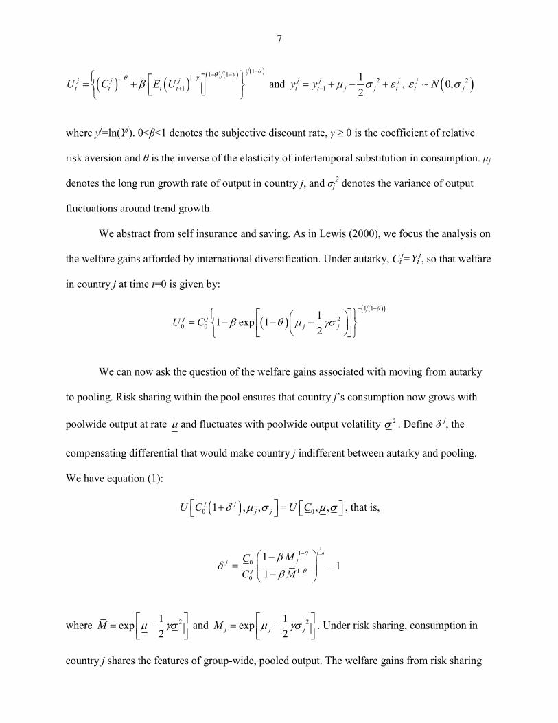
( ) ( )( ) ( ) ( )1 11 11 1

1j j j

t t t tU C E Uθθ γθ γ

β−− −− −

+

⎧ ⎫⎡ ⎤= +⎨ ⎬⎢ ⎥⎣ ⎦⎩ ⎭ and 2

112

j j jt t j j ty y μ σ ε−= + − + , ( )2~ 0,j

t jNε σ

where yj=ln(Yj). 0<β<1 denotes the subjective discount rate, γ ≥ 0 is the coefficient of relative

risk aversion and θ is the inverse of the elasticity of intertemporal substitution in consumption. μj

denotes the long run growth rate of output in country j, and σj2 denotes the variance of output

fluctuations around trend growth.

We abstract from self insurance and saving. As in Lewis (2000), we focus the analysis on

the welfare gains afforded by international diversification. Under autarky, Ctj=Yt

j, so that welfare

in country j at time t=0 is given by:

( )( )( )1 1

20 0

11 exp 12

j jj jU C

θ

β θ μ γσ− −

⎧ ⎫⎡ ⎤⎛ ⎞= − − −⎨ ⎬⎜ ⎟⎢ ⎥⎝ ⎠⎣ ⎦⎩ ⎭

We can now ask the question of the welfare gains associated with moving from autarky

to pooling. Risk sharing within the pool ensures that country j’s consumption now grows with

poolwide output at rate μ and fluctuates with poolwide output volatility 2σ . Define δ j, the

compensating differential that would make country j indifferent between autarky and pooling.

We have equation (1):

( )0 01 , , , ,j jj jU C U Cδ μ σ μ σ⎡ ⎤ ⎡ ⎤+ = ⎣ ⎦⎣ ⎦ , that is,

where 21exp2

M μ γσ⎡ ⎤= −⎢ ⎥⎣ ⎦ and 21exp

2j j jM μ γσ⎡ ⎤= −⎢ ⎥⎣ ⎦. Under risk sharing, consumption in

country j shares the features of group-wide, pooled output. The welfare gains from risk sharing

111

01

0

11

1jj

j

MCC M

θθ

θ

βδ

β

−−

−

⎛ ⎞−= −⎜ ⎟⎜ ⎟−⎝ ⎠

8

has three components. First, pure diversification gains, i.e. the difference between individual and

poolwide volatilities, jσ and σ . Second, growth differentials, i.e., the difference between

growth rates within and without the pool, μ and jμ . Third, the ratio between initial

consumption in autarky, 0jC , and initial consumption in the pool, 0C . This term reflects a

(positive or negative) “entry transfer” in terms of the initial consumption that country j pays to

(or receives from) other members for being allowed into the pool. Obstfeld (1994) focuses on

diversification and growth welfare gains, and sets 0 0jC C= .

Of course, welfare gains can also result from self-insurance, via saving and borrowing

decisions, rather than internationally. We do not mean to suggest either approach dominates.

Rather the paper follows the international risk-sharing literature and investigates how quickly

welfare gains accrue when insurance is sought exclusively via international contracts.

Solving for entry transfers, Lewis (2000) shows that

10

0

11

jj

j

HC MC M M H

θ

θ

ββ

−

−

−=

−

where 212exp cov( , )j

j j t tH μ γσ γ ε ε⎡ ⎤= + −⎣ ⎦ and jt t

j

ε ε=∑ .5 H reflects the desirability of

country j from the standpoint of the pool’s hedging motive. Countries characterized by low (or

negative) covariance with the pool will be more likely to receive a net transfer at the beginning

of the arrangement ( 0 0jC C< ). Conversely, countries whose output covaries strongly with

poolwide output will be more likely to make a net payment in order to join the pool (that

is, 0 0jC C> ). These transfers ensure that risk sharing is Pareto-improving. Countries whose

growth or volatility performances worsen upon entry in a given pool are compensated, so that

5 An approximation is necessary here, that assumes the sum of log-normal processes continues to be distributed log-normally. Lewis (1996) presents Monte-Carlo evidence suggestive the assumption is relatively innocuous.

9

consumption insurance cannot make them worse off. Perfect risk sharing is a first-best

equilibrium for each given pool size. Of course, the overall first-best obtains for all countries

sharing risk. Here, we ask how many parties are necessary to achieving the bulk of the first-best

gains. The question becomes relevant if risk sharing arrangements entail monitoring costs that

increase with the size of the membership.

For a given country j, the total welfare gains associated with joining a pool of countries

with average growth μ and volatility σ is given by equation (2):

( ) ( )1

1 11 11 11

1jjj

j

M MHM M H

θθ θθ θ

θ

β βδ

β

− −− −

−

− −= −

−

The gain associated with a pooling arrangement taken as a whole is given by a weighted average

of jδ for all countries j in the pool. In appendix A, we show that under relatively mild

assumptions, the expression for total poolwide welfare simplifies considerably. In particular,

with no outlier country in the time average of growth or volatility,

( ) ( )

( ) ( )

1 11

1 11

11

1

N

j jNjj

jj

M

M

θθ

θθ

ω βω δ

β

−−

−−

−−

−

∑∑

with 0

0

j

j Nj

j

Y

Yω =

∑. In other words, total poolwide welfare gains are approximately given by a

weighted average of the pure volatility and growth gains obtained when setting 0 0jC C= in

equation (1), i.e., shutting entry transfers down. With no country outliers for the time average of

output growth and volatility, transfers across the pool approximately cancel out. The result

remains valid for any weights.

This has important consequences for the questions we are asking. It suggests a weighted

average of all countries’ growth and volatility gains will approximate well poolwide welfare

10

gains. So long as countries with extreme growth or volatility performances are excluded, a

weighted sum of the volatility and growth changes for all countries in a pool will be close to the

true gains given in equation (2). We later confirm that, for most samples, computing the

empirical counterpart to 0

0j

CC

does not alter substantially the measured poolwide welfare gains.

For economies with growth and volatility not too distant from the sample cross-sectional

average, focusing on the changes in volatility and in growth induced by accession to a given risk

sharing pool—as Obstfeld (1994) does—can be illustrative of the overall welfare gains.

In what follows, we compare how countries fare individually and under pooling, using

four approaches. First, we report the standard deviation of the growth rate for individual country

GDP and its poolwide counterpart. This simple approach, focused on pure diversification gains,

conveys most of the key economic intuition. Second, we compute the implied welfare gains

assuming expected growth is the same for all countries (μ = jμ ) and abstracting from entry

transfers ( 0jC = 0C ). These simplifying assumptions make it possible to focus narrowly on the

welfare implications of the fall in volatility associated with pooling, and follow directly from

Obstfeld (1994). There, the emphasis is on the implications of reducing or eliminating volatility,

rather than on entry transfers. Under this approach, welfare is a monotonic, non-linear

transformation of volatility.

Third, we report welfare allowing for entry transfers. More specifically, we compute total

welfare gains as the income-weighted sum of δj across the membership, as implied by equation

(2). Fourth and finally, in Section V we relax the assumption that growth rates are the same for

all countries, and project μ and jμ using past observed growth rates. The paper thus follows a

variety of alternative approaches, and does so for two reasons. First, we aim to provide a

transparent presentation of where the gains are coming from. Second, and perhaps more

11

important, views may differ regarding the realism of the various components of a risk-sharing

contract, e.g. the market determination of entry transfers, or the provision of insurance against

differences in long-run growth as opposed to temporary fluctuations.

As is well known, the link between welfare and volatility depends on some key properties

of the process generating uncertainty: in particular, insurance against permanent shocks has more

value than against temporary ones (see, for instance, Obstfeld, 1994). We assume throughout that

shocks to consumption follow a random walk. The assumption is only maintained so that we can

decompose poolwide variances into meaningful elements (Section III.B). Under trend

stationarity, the variance of the poolwide residual is not the variance of a sum of each member

country’s residual, and the difference between the two has no reason to be negligible.

The random walk assumption is in fact not crucial to our results, as we now explain.

Under the alternative assumption of trend stationarity, measured uncertainty is always higher.

Indeed, if the true process for GDP has a unit root, the detrended residual will have explosive

variance. If on the other hand the true process is trend stationary, the measured variance of GDP

growth will be lower than the true residual variance. In both cases, measured volatility is higher

when assuming trend stationarity. But under trend stationarity, the welfare costs of fluctuations

are smaller for a given level of uncertainty. As is well known from Lucas’ (1987) seminal paper,

the welfare costs of fluctuations are then approximately given by 21

2γσ , where γ is the coefficient

of risk aversion and σ2 denotes the variance of residual uncertainty. The two effects on end

welfare tend to offset one another. In fact, we ran our search algorithm under the assumption of

trend stationarity, and found similar results, not reported for the sake of brevity. We reproduced

almost identically the general shape of minimum variance envelopes for the various country

groupings, and the relative impact of different types of constraints on the universe of countries

that one can pool with. The key simplification for our purposes is therefore that the same type of

12

process (either stationary or random walk) applies to all countries—an assumption that may

prove difficult to invalidate, given the weakness of standard unit root tests.6

B. Combinatorial Analysis

Searching for pools of countries that yield the lowest possible variance of the growth rate

of aggregate (poolwide) GDP is not straightforward, in light of the vast number of possible

combinations of countries. We consider the N countries in our sample individually, then all of

their possible combinations 2 countries at a time (which equals 2NC ), then 3 at a time (which

equals 3NC ), and so on, where

( )!

! !Np

NCp N p

=−

. As is well known, the total number of

partitions is 1

2 1N

N Np

p

C=

= −∑ , which quickly reaches astronomical levels as N rises.

Using a computational algorithm whose details are provided in a Technical Appendix

available upon request, we are able to keep track of all possible combinations for any pool size

within a universe of 31 countries, i.e. 2.1 billion combinations. This algorithm can easily handle,

for example, the universe of 26 emerging market countries—about 67 million combinations.

However, when the universe consists of all 74 countries in our sample, the same algorithm only

allows us to analyze all combinations of pools of size 7 or less ( 747C = 1.8 billion). By symmetry,

we can also draw the inventory of all combinations of size 67 or above, since N Np N pC C −= . Beyond

these, we need to resort to an approximation algorithm. When N = 74, the total number of groups

increases to 274=1.9x1022, too large for existing computing power. For each group, one needs to

sum the GDP levels for all countries in the pool, to compute an aggregate growth rate and the

6 Dezhbakhsh and Levy (2003) use frequency analysis to investigate the cross-section of spectra followed by GDP growth rates. They find substantial heterogeneity, but are unable to point to a key determining factor. Aguiar and Gopinath (2007) suggest that the random walk assumption may be more appropriate for emerging markets than for advanced countries.

13

corresponding standard deviation. Even if each operation took a nanosecond to complete,

running an exhaustive search over all possible pools amongst 74 countries would take hundreds

of centuries.

Approximation method for large samples

For sample sizes where exhaustive inventories are out of reach, we implement recursive

searches. Combinatorial problems similar to those we are tackling are the object of a large

literature in computer sciences revolving around the so-called “Traveling Salesman” problem,

for which well-established approximated solution methods exist. To our knowledge however

none can be applied to our baseline setup. For instance, Han, Ye and Zhang (2002) propose an

approximation algorithm that can be applied to minimize the variance of a sum; but we minimize

the variance of a weighted sum, where the weights themselves depend on the group’s

membership. In Imbs and Mauro (2007), we use the Han, Ye and Zhang (2002) algorithm to

identify risk diversification benefits for a given absolute size of the risk-sharing contract (for

example, a US$1 contract). That exercise involves an unweighted average of GDP growth rates.

Our conclusions are virtually identical.

We first obtain all possible combinations up to the maximum pool size where this is

feasible through an exhaustive search—in our case, all pools of size 7 drawn from the universe

of 74 countries. We save not only the best pool of size 7, but also the best W pools of size 7 that

include each of the N countries in the universe under consideration. In our baseline results, we

use W=1351 (74 times 1351 is just below 100,000).

For each of these W N⋅ “seed” pools, we analyze all groups that include the existing

members, plus one of the ( N p− ) remaining countries. Among these, we find the best pool of

size 8 (as well as the W N⋅ best new “seed” pools of size 8). We iterate the procedure. Although

there is a recursive aspect to this, the fact that at each stage we consider the best W pools for each

14

of the N countries gives plenty of opportunities for countries that are in the best pool of a given

size to drop out at the next increment.

We have verified the reliability of this approximation in four different ways. First, for a

number of the cases where it is possible to run exhaustive searches, we compared the groupings

implied by an exhaustive inventory to the results of our approximation: they were always

identical. Second, we have experimented with different values for W, as low as 2, and have found

systematically the same results as with W=1351. Third, for each pool size p, we have checked

large numbers of random samples of countries. We have not found a single instance in which a

pool drawn randomly was preferable to those identified as the best through the approximation

procedure. Fourth, we have run exhaustive searches for all possible combinations of 67 (or more)

countries selected amongst 74. Again, we have found the same optimal pools as those obtained

by running the approximation procedure throughout.

III. RESULTS

In this section we describe our dataset and present our results. We first build intuition

through a simple, single country example. We then present our main results, pertaining to a

“global envelope” of the groupings that achieve maximal risk-sharing gains for all group sizes.

A. Data

Data on yearly real gross domestic product and consumption, evaluated in purchasing

power parity (PPP) U.S. dollars, for the period 1974–2004 are drawn from the World Bank’s

World Development Indicators. Compared with the widely used Penn World Tables (PWT), the

World Bank data base has similar quality, and in fact builds on usually identical information. But

it provides PPP-adjusted data until 2004 rather than 2000. We cross-checked the two data bases

over the period covered by both, and are confident the results are largely unaffected if we use

PWT.

15

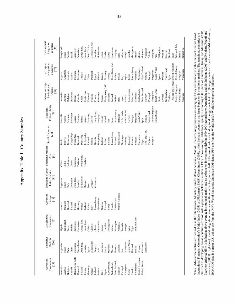
This yields a sample of 25 advanced countries, 26 emerging market countries, and 23

developing countries with complete coverage and data of reasonable quality. (The full country

list is provided in Appendix Table 1). Advanced countries are defined as in the International

Monetary Fund’s World Economic Outlook. The remaining countries are considered emerging if

they are included in either the stock-market-based International Financial Corporation’s Major

Index (2005), or JPMorgan’s EMBI Global Index (2005), which includes countries that issue

bonds on international markets. The rest are classified as developing.

Throughout the paper, in line with the bulk of the literature on international risk sharing,

we assume that PPP holds. This corresponds to the notion that risk sharing is contracted on a pre-

agreed exchange rate, possibly one that is expected to prevail in the long run. While standard,

this is an important assumption. Previous studies (for example, Backus and Smith, 1993; and

Ravn, 2001) have established that real exchange rate fluctuations worsen the case for

international risk sharing. Indeed, GDP data at market exchange rates would imply far higher

volatility—harder to hedge through international risk sharing. To compute trade integration, the

data on exports (in U.S. dollars at current prices) are drawn from the IMF’s Direction of Trade

Statistics, and the data on GDP (in U.S. dollars at current prices) are from the IMF’s World

Economic Outlook database.

B. A Simple Example

To develop intuition, we begin by asking what pools of countries minimize risk from the

standpoint of an individual country, chosen as an example to illustrate the general approach. We

work through the case of Chile, viewed by international investors as a relatively safe emerging

market (as reflected in low sovereign spreads), and whose growth and volatility experience is not

an outlier. Chile is not participating in existing or prospective reserve-pooling arrangements and

16

its economy is not overwhelmingly linked to a single or a few other countries. The general

pattern of results holds for all other countries, as will become apparent in the next section.

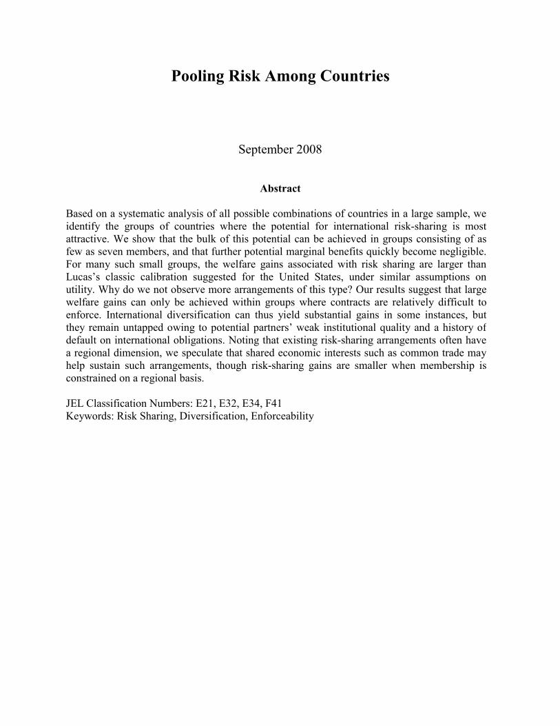
For each pool size, Figure 1 plots the standard deviation of the growth rate of poolwide

GDP for the best groups of countries (from the standpoint of volatility) that contains Chile,

chosen among all 74 countries. We also show these envelopes for various restrictions on the

universe of potential partners Chile can choose from. In particular, we present the cases when

Chile can pool only with other emerging markets, developing countries, or advanced economies.

To give a sense of the importance of choosing well one’s risk-sharing partners, we also plot the

highest-standard-deviation envelope (that is, the least desirable pools from Chile’s standpoint,

for each pool size) among the 74 countries.

Several results deserve mention. First, the lowest possible standard deviation for

poolwide GDP growth in a group that includes Chile is 0.61 percentage points, far below the

4.41 percentage points for Chile on its own. As it turns out, this obtains for a group of 20

countries. Second, a small number of carefully chosen partners is sufficient to yield the bulk of

available risk-sharing benefits. Even with just one well-chosen partner (in this case, France),

poolwide standard deviation falls to 1.26 percentage points. The standard deviation of GDP

growth reaches 0.72 percentage points, already quite close to the minimum, for the best pool of 7

members.

Not surprisingly, this is a motley set of economies: Austria, Cameroon, Chile, New

Zealand, Nicaragua, Sweden, and Syria.

As will become apparent, the finding that most diversification gains can be attained in

relatively small pools holds for all countries. In the United States for instance, despite the large

size of the U.S. economy, pooling with another five or six well-chosen economies (including

Japan, in the first instance) implies a near halving of US volatility. This result is reminiscent of

17

the well-known finding in finance that a small set of stocks is often sufficient to provide most of

the diversification opportunities available from a market portfolio (Solnik, 1974).

This is a Pareto improvement compared with the status quo: focusing exclusively on

volatility reduction, each of the countries included is far better off in this pool than on its own.

Indeed, the lowest-standard-deviation envelope shown in Figure 1 looks almost identical if one

adds the constraint that pools should be Pareto improving, i.e. that volatility be lower for all

participants under pooling than in autarky.

Marginal gains quickly become small. Based on the volatility criterion they become

negative for groups above 20 members, and more visibly negative as the pool size

increases further than, say, 30 members. Beyond a certain pool size, covariance benefits

are no longer significant, and the pool starts having to include countries whose volatilities

are far higher than the sample average. With the introduction of these increasingly volatile

countries, the approximation developed in section II.A is decreasingly valid. In particular,

the welfare gains from a pooling arrangement are increasingly distinct from changes in

volatility, because transfers do not sum to zero across the pool any longer. These highly

volatile countries need to pay (and are willing to pay) entry transfers to the rest of the pool

to gain admission. Membership to the pool is Pareto-superior and welfare increases

because of gains to financial trade, despite a concomitant rise in poolwide volatility. This

will become clearer in Section II.C.

Finally, the (upper) envelope corresponding to the worst possible pools of each size

highlights the importance of choosing one’s partners carefully: at small pool sizes, one runs the

risk of achieving higher volatility in a poorly chosen pool than in autarky. In the paper, we

sometimes note, but typically do not focus on, the exact identities of the countries that form the

best group. In general, poolwide uncertainty for the lowest volatility group is only marginally

18

below that for the groups with the second or third lowest volatilities (or even higher). Given that

the differences are so small, it is likely that considerations outside our analysis may lead

countries not to choose the absolute best.

We emphasize the extent to which various types of (economically relevant) constraints

may reduce the maximum possible risk diversification benefits. For example, Figure 1 also

reports the extent to which possible gains decline when the universe of countries that Chile can

choose from is constrained by the level of economic and financial development, or

geographically. The lowest possible standard deviation amounts to 0.61 percentage point when

Chile is allowed to choose its pooling partners among all 74 countries, but 0.87 percentage point

when it is constrained to pool with advanced countries only, 1.07 percentage point within the

universe of emerging markets only, and 1.91 percentage points when pooling within Latin

America only. Risk-sharing agreements that are based on common geographic origins, or

restricted to countries within a given range of per capita income, provide smaller gains than do

pools formed by choosing from the unconstrained, worldwide sample.

Variance Decomposition

To illustrate the sources of risk diversification gains, it is useful to decompose the

variance of the growth rate of poolwide GDP into a weighted average of the variances of

individual countries’ growth rates and a weighted sum of all bilateral covariances:

2

1 1 1

( ) ( ) ( ) ( , )p p p p

p i i i i i j i ji i i j

Var g Var w g w Var g w w Cov g g= = =

= = +∑ ∑ ∑∑ for ; 1,...i j i p≠ =

where wi denotes the share of country i in the pool’s production, gp is the growth of aggregate

GDP for a pool of p countries, and individual countries’ growth rates are denoted by gi.

Countries are attractive partners to the extent that they have low variances and low (or, even

better, negative) covariances with other members of the pool.

19

Decomposing poolwide variance for the “best” pool of each pool size, it is possible to

show (as we do in Imbs and Mauro, 2007) that diversification gains for pool sizes up to about

seven countries stem from both the addition of countries with lower volatility than Chile’s and

low (or negative) covariances. The first few countries have both low individual variances and

negative covariances with Chile (as well as, importantly, with each other). However, the

covariance gains diminish rapidly, as the sum of all bilateral covariances starts increasing again.

From pool size of about seven onwards, the remaining diversification gains are accounted for

almost exclusively by the addition of countries with lower variance than Chile, but not with

negative average covariances with the rest of the membership.

The results presented in this section are confirmed and generalized in the next. On the

basis of risk diversification alone, there is little need for arrangements including many countries,

as long as partners are chosen carefully. Welfare gains can in principle be sizeable even in small

pools formed on a regional basis or where membership is constrained to countries with relatively

low economic development. However, pools that deliver the greatest diversification benefits tend

to consist of heterogeneous countries with respect to geography, as well as economic and

financial development.

C. Global Diversification

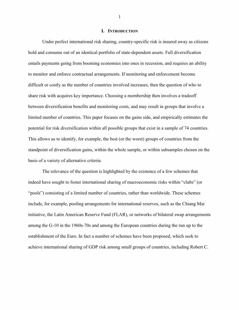
We now generalize our results in an exercise that no longer restricts optimal pools to

include any given country: Figure 2 reports the envelope of minimal volatility for all pool sizes p

up to 74. As in the previous section, the bulk of possible diversification gains is attained with

relatively small pools. The global best using the pure volatility criterion is a pool of 17 countries,

which delivers a standard deviation equal to 0.50 percentage points.7 However, the standard

7 Austria, Bangladesh, Benin, Botswana, Cameroon, Chile, Rep. Congo, Costa Rica, Dominican Republic, El Salvador, Gambia, Iceland, Kenya, Lesotho, New Zealand, Nicaragua, Senegal, Sweden, Syrian Arab Republic, and Zimbabwe.

20

deviation is already as low as 0.62 percentage points for the best pool of size 7.8 The property

that diversification gains are achieved within groups consisting of a small number of countries

continues to prevail in this general setup.

The value reported for p=1 corresponds to the standard deviation of the individual growth

rate for the least volatile country during the sample period, namely France. Diversification gains

for specific countries cannot be easily read off the figure, because the identities of countries

involved in the various optimal pools of different sizes may change. But we know the identities

of the relevant groupings, and can thus assess the gains that optimal pooling would provide to

member countries. For example, in the case of the optimal group of size 7, the standard

deviations of individual countries’ growth rates range from 1.44 percentage points for Sweden to

8.97 percentage points for Nicaragua. The diversification gains are distributed unequally, with

far larger gains accruing to countries with more volatile individual growth rates. This asymmetry

has implications for entry transfers.

The list of countries involved in optimal pools confirms that heterogeneity is key.

Interestingly, the list overlaps quite substantially with that obtained for the case of Chile. Several

of the same countries come up as members of the best pools of smaller sizes (where we run a

search over all possible pools, without any approximation) and continue to be present throughout

all optimal pools for p>7. Again, this is unlikely to be an artifact of our approximation method,

despite the recursive structure it imposes onto the search, because the procedure leaves plenty of

opportunities for countries to drop out of the best pool as size increases. Rather, the evidence

suggests that the sample of countries providing the best mutual hedging properties within a

universe of 74 economies is relatively small and robust. For example, the country with lowest

individual volatility, France, does not enter any of the “best” groupings, likely because its growth 8 Austria, Colombia, Costa Rica, Dominican Republic, New Zealand, Nicaragua, and Sweden.

21

cycle is highly correlated with many other economies in the sample. This reinforces the

empirical relevance of low (or negative) covariances.

Figure 2 also reports the minimum standard deviation of the poolwide growth rate for

sub-samples constrained to the advanced countries, emerging markets, and developing countries.

While risk diversification gains are substantial within each sub-sample, they are not as large as in

the full universe of countries. The envelopes for emerging and developing economies are roughly

one percentage point above the global envelope, for all p. For p<3, the global envelope and that

corresponding to advanced economies coincide, but for larger pool sizes even advanced

countries are considerably better off in pools that allow them to share risk with emerging or

developing countries. Advanced economies achieve somewhat smaller gains, which is consistent

with their lower volatility and internationally correlated business cycles. The rapid exhaustion of

diversification opportunities continues to hold in all three sub-samples.

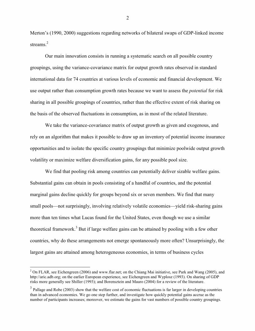
Welfare Gains

We now turn to welfare, and allow 0 0jC C≠ . We still constrain the expected growth rate

to be the same for all countries—an assumption we relax in Section V. Figure 3 reports the

highest (total income-weighted) welfare gains 1

Nj

jjω δ

=∑ for any pool size N. The total gains are

monotonically increasing with pool size, and attain a maximum when the entire (sub-)universe of

countries under consideration are pooling together. Just as volatility decreased rapidly in the

number of member countries, welfare gains are large for small-sized groupings. Marginal gains

peter out for pools beyond seven or eight members. Again, the rapid decline in marginal welfare

gains holds when the exercise is conducted for sub-samples of countries consisting of only

advanced, emerging, or developing countries.

22

The pool formed by the entire 74-country sample for which we have data delivers total

gains amounting to 1.9 percent of initial worldwide income (Table 1). Even allowing for entry

transfers, the gains are far larger for those groups of countries that start out with higher volatility

prior to pooling. As a share of initial income for the group under consideration, total (income-

weighted) welfare gains amount to 0.7 percent for advanced countries, 4.4 percent for emerging

markets and up to 7.4 percent for developing countries. Welfare gains are relatively small in rich

countries simply because they are less volatile. Table 1 shows the size of these gains differs

considerably, depending on the country’s individual volatility under the status quo. In the full

sample, the minimum (United States) annual gains amount to 0.5 percent of initial country

income, and the median gain (Dominican Republic) is 4.1 percent.

To construct Figure 3, we chose β=0.95, consistent with a 5% annual discount rate, θ=2

and γ=5. We experimented extensively with alternative values for these parameters.

Unsurprisingly, higher values for γ or β shifted upwards the magnitude of the welfare gains we

computed for all poolsizes. But the overall shape of Figure 3 never altered. In particular, the fact

that most welfare gains accrue within very small groups of countries always obtained.

IV. POOLING RISK WITHIN SUB-SAMPLES

In this section we quantify the foregone diversification and welfare gains implied by the

need to choose one’s pooling partners within specific sub-samples. In particular, we seek to

assess the importance of choosing partner countries for whom contract enforcement and

monitoring may be relatively easy. We approximate the concept in a variety of ways, splitting

our sample according to: (a) the level of development and country size; (b) institutional quality

and past repayment record on international debt obligations; (c) the degree of international

financial integration; (d) geographical region; and (e) bilateral trade intensity. In all these cases,

we present the results based on simple volatility criteria, as well as welfare computed with and

23

without entry transfers. We report the main results in Table 2, for the best possible pool of any

size. We also consider existing risk-sharing schemes such as the Chiang-Mai Initiative or FLAR,

or other types of existing arrangements whereby participants have long established

cooperation—for example, in the context of a currency union or a trade agreement. We estimate

the extent to which participant countries would be able to obtain larger welfare gains in pools of

the same size if they were to choose their partners in an unconstrained manner.

In undertaking these exercises, we assume that the variance-covariance matrix of

international output growth rates would not be affected by entering international risk-sharing

arrangements. This is consistent with findings by Doyle and Faust (2005). They show that,

despite claims that rising integration among the G-7 economies has increased cycles

synchronization, there is no evidence of a significant increase in the correlation of output growth

rates or other macroeconomic aggregates. Moreover, a large empirical literature has documented

the cross-sectional properties of international business cycles, which appear to have extremely

persistent determinants, such as trade linkages or patterns of production (see Frankel and Rose,

1998 or Baxter and Kouparitsas, 2005). These results are consistent with our assumption that the

international covariances in output growth rates are largely time-invariant.

A. Level of Development and Country Size

The degree of volatility reduction and welfare gains that can be attained by pooling

countries within categories defined on the basis of the level of economic development is

informative in two respects. First, it helps gauge the potential interest in pooling risk on the part

of countries belonging to different income groups. Second, countries may be more likely to

engage in risk sharing agreements with members of a similar income group.

In Table 2, we first report for each sub-sample the median value of the standard deviation

of individual countries’ growth rates across the countries within the sub-universe. Then, for each

24

country we search over all possible pools of any size that it can form together with others chosen

within the sub-sample. We note the lowest achievable standard deviation of poolwide growth,

and report in the second column the median value of that standard deviation across all countries

in the sub-sample. We then compute for each country the welfare gain obtained by joining its

best pool, assuming that all countries have the same expected growth rate and that there are no

entry transfers, following Obstfeld (1994). Again, we impose γ = 5, θ = 2, and β = 0.95. Our

main conclusions hold for alternative values. We report in the third column the median value of

these gains across countries in the sub-universe. Finally, we allow entry transfers and report the

sum of the income-weighted welfare gains that would obtain if all countries in the sub-universe

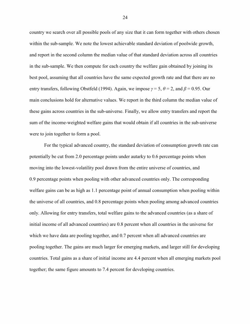
were to join together to form a pool.

For the typical advanced country, the standard deviation of consumption growth rate can

potentially be cut from 2.0 percentage points under autarky to 0.6 percentage points when

moving into the lowest-volatility pool drawn from the entire universe of countries, and

0.9 percentage points when pooling with other advanced countries only. The corresponding

welfare gains can be as high as 1.1 percentage point of annual consumption when pooling within

the universe of all countries, and 0.8 percentage points when pooling among advanced countries

only. Allowing for entry transfers, total welfare gains to the advanced countries (as a share of

initial income of all advanced countries) are 0.8 percent when all countries in the universe for

which we have data are pooling together, and 0.7 percent when all advanced countries are

pooling together. The gains are much larger for emerging markets, and larger still for developing

countries. Total gains as a share of initial income are 4.4 percent when all emerging markets pool

together; the same figure amounts to 7.4 percent for developing countries.

25

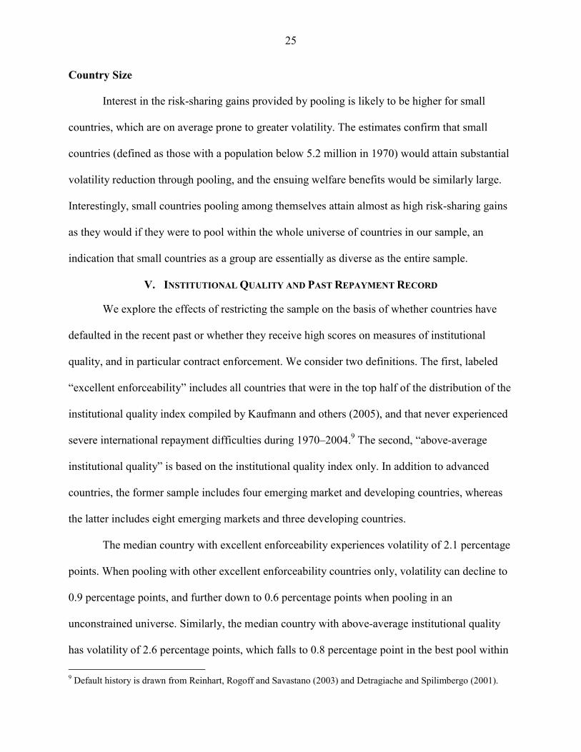
Country Size

Interest in the risk-sharing gains provided by pooling is likely to be higher for small

countries, which are on average prone to greater volatility. The estimates confirm that small

countries (defined as those with a population below 5.2 million in 1970) would attain substantial

volatility reduction through pooling, and the ensuing welfare benefits would be similarly large.

Interestingly, small countries pooling among themselves attain almost as high risk-sharing gains

as they would if they were to pool within the whole universe of countries in our sample, an

indication that small countries as a group are essentially as diverse as the entire sample.

V. INSTITUTIONAL QUALITY AND PAST REPAYMENT RECORD

We explore the effects of restricting the sample on the basis of whether countries have

defaulted in the recent past or whether they receive high scores on measures of institutional

quality, and in particular contract enforcement. We consider two definitions. The first, labeled

“excellent enforceability” includes all countries that were in the top half of the distribution of the

institutional quality index compiled by Kaufmann and others (2005), and that never experienced

severe international repayment difficulties during 1970–2004.9 The second, “above-average

institutional quality” is based on the institutional quality index only. In addition to advanced

countries, the former sample includes four emerging market and developing countries, whereas

the latter includes eight emerging markets and three developing countries.

The median country with excellent enforceability experiences volatility of 2.1 percentage

points. When pooling with other excellent enforceability countries only, volatility can decline to

0.9 percentage points, and further down to 0.6 percentage points when pooling in an

unconstrained universe. Similarly, the median country with above-average institutional quality

has volatility of 2.6 percentage points, which falls to 0.8 percentage point in the best pool within 9 Default history is drawn from Reinhart, Rogoff and Savastano (2003) and Detragiache and Spilimbergo (2001).

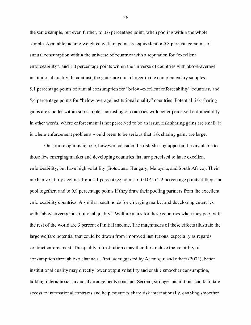
26

the same sample, but even further, to 0.6 percentage point, when pooling within the whole

sample. Available income-weighted welfare gains are equivalent to 0.8 percentage points of

annual consumption within the universe of countries with a reputation for “excellent

enforceability”, and 1.0 percentage points within the universe of countries with above-average

institutional quality. In contrast, the gains are much larger in the complementary samples:

5.1 percentage points of annual consumption for “below-excellent enforceability” countries, and

5.4 percentage points for “below-average institutional quality” countries. Potential risk-sharing

gains are smaller within sub-samples consisting of countries with better perceived enforceability.

In other words, where enforcement is not perceived to be an issue, risk sharing gains are small; it

is where enforcement problems would seem to be serious that risk sharing gains are large.

On a more optimistic note, however, consider the risk-sharing opportunities available to

those few emerging market and developing countries that are perceived to have excellent

enforceability, but have high volatility (Botswana, Hungary, Malaysia, and South Africa). Their

median volatility declines from 4.1 percentage points of GDP to 2.2 percentage points if they can

pool together, and to 0.9 percentage points if they draw their pooling partners from the excellent

enforceability countries. A similar result holds for emerging market and developing countries

with “above-average institutional quality”. Welfare gains for these countries when they pool with

the rest of the world are 3 percent of initial income. The magnitudes of these effects illustrate the

large welfare potential that could be drawn from improved institutions, especially as regards

contract enforcement. The quality of institutions may therefore reduce the volatility of

consumption through two channels. First, as suggested by Acemoglu and others (2003), better

institutional quality may directly lower output volatility and enable smoother consumption,

holding international financial arrangements constant. Second, stronger institutions can facilitate

access to international contracts and help countries share risk internationally, enabling smoother

27

consumption for a given degree of output volatility. The results presented in this section suggest

that this second channel has the potential to improve welfare substantially.

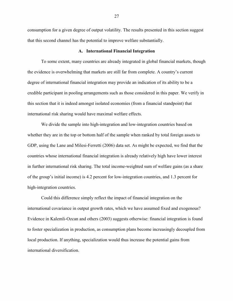
A. International Financial Integration

To some extent, many countries are already integrated in global financial markets, though

the evidence is overwhelming that markets are still far from complete. A country’s current

degree of international financial integration may provide an indication of its ability to be a

credible participant in pooling arrangements such as those considered in this paper. We verify in

this section that it is indeed amongst isolated economies (from a financial standpoint) that

international risk sharing would have maximal welfare effects.

We divide the sample into high-integration and low-integration countries based on

whether they are in the top or bottom half of the sample when ranked by total foreign assets to

GDP, using the Lane and Milesi-Ferretti (2006) data set. As might be expected, we find that the

countries whose international financial integration is already relatively high have lower interest

in further international risk sharing. The total income-weighted sum of welfare gains (as a share

of the group’s initial income) is 4.2 percent for low-integration countries, and 1.3 percent for

high-integration countries.

Could this difference simply reflect the impact of financial integration on the

international covariance in output growth rates, which we have assumed fixed and exogenous?

Evidence in Kalemli-Ozcan and others (2003) suggests otherwise: financial integration is found

to foster specialization in production, as consumption plans become increasingly decoupled from

local production. If anything, specialization would thus increase the potential gains from

international diversification.

28

B. Regional Constraints

In practice, existing or prospective pools are often formed on a regional basis. We

analyze the implications of geographical constraints through a few examples. We estimate the

gains that the advanced European countries would obtain if they were only allowed to pool with

other advanced European countries, and compare them to the gains that would obtain if they

were allowed to pool with all other advanced countries without geographic restrictions.

Similarly, we compare the gains available to emerging Asia or, separately, Latin America, with

the gains obtained within the sample of all emerging markets.

Geographical constraints do not turn out to be very important for advanced European

countries, presumably because they constitute a high proportion of advanced countries, and

because the advanced country cycle has a large worldwide common component. The median

advanced European country can cut its volatility from 1.8 percentage points to 1.0 percentage

point in a pool of advanced European countries, and to a rather similar 0.9 percentage point in a

pool of advanced countries chosen worldwide. The same message holds for welfare gains.

In contrast, geographical constraints are more relevant for emerging markets’ ability to

diversify risk. For instance, median volatility for individual Latin American emerging markets

equals 4.4 percentage points and can be lowered to 1.9 percentage point by pooling with five

well chosen Latin American emerging markets, but to as low as 1.3 (1.1) percentage point by

pooling with five (ten) emerging markets in the absence of geographical constraints. Similarly,

the median Asian emerging market can reduce its volatility from 3.6 percentage points to 1.8

percentage points in a pool of seven Asian emerging markets, and to 1.1 percentage points in a

pool of ten emerging markets chosen also from outside the region. The impact of geographical

constraints remains substantial, although it becomes smaller, when measured in terms of welfare.

For Latin American emerging markets, welfare gains can amount to 5.4 percentage points of

29

initial income when pooling within the whole universe of emerging markets, but also gains of

4.1 percentage points when pooling within emerging Latin America. Asian emerging markets

can obtain welfare gains equivalent to 3.6 percentage points of initial income when pooling

within the whole universe of emerging markets, but also gains of up to 3.0 percentage points

when pooling within emerging Asia.

In Imbs and Mauro (2007), we show that the costs of regional constraints are even greater

when measured using the number of instances in which countries in a group are simultaneously

affected by pressures on the exchange rate. This is consistent with studies that find a substantial

regional element in currency crises and in international contagion more generally (Glick and

Rose, 1999).

C. Trade Integration

In this sub-section, we explore further the theme of contract enforceability, which we

relate to trade patterns and the associated regional element often observed in actual pooling

arrangements. On the one hand, trade linkages imply higher output correlations and thus reduced

diversification possibilities. But on the other hand, they presumably induce a greater ability to

enforce risk-sharing contracts, because defaulting partners can be sanctioned via exclusion from

goods trade (see, for example, Rose and Spiegel, 2004). This may explain the regional element

observed in actual pooling arrangements, which suggests that the positive impact on contract

enforceability may in some cases prevail over the negative impact on diversification

opportunities.

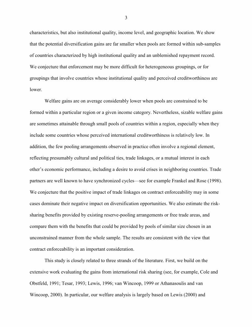
To measure trade integration within a pool, we sum exports across all pool members as a

ratio to poolwide GDP. We then consider all possible pools and analyze the correlation between

this measure of trade integration with the minimal volatility of poolwide output. As is well

known, trade is substantially lower among emerging markets than it is among advanced

30

countries, and it is even lower among developing countries. We analyze separately the

relationship between trade integration and poolwide output volatility for all possible pools of (i)

advanced economies, (ii) emerging markets, and (iii) developing countries. The relationship is

depicted in Figure 4 for pool sizes 5 and 10. The results suggest that greater trade integration is

clearly associated with larger minimal poolwide volatility within the universe of emerging

markets and, separately, developing countries. In other words, fewer diversification opportunities

are available among trade partners. The relationship is weaker among advanced economies,

where risk-sharing gains are smaller to begin with.

The few instances of effective risk sharing arrangements we observe have tended to

involve regional trade partners. This limits substantially the potential diversification gains, as

shown above. Trade relations must then present an offsetting advantage: we conjecture that trade

helps leverage the enforcement of international commitments, because of the dynamic threat of

exclusion.

D. Existing Arrangements

Finally, we consider the potential welfare gains arising from existing risk-sharing

arrangements such as the Chiang-Mai Initiative or FLAR. We also discuss other types of

international agreements, whereby participants have long-established cooperation, for example,

in the context of a currency union or a trade agreement. We then compare such gains to those

that the participant countries would be able to obtain in pools of the same size, drawing their

partners from the whole, unconstrained sample. The objective here is not to assess the

desirability of existing arrangements, but rather to assess the value of well-established relations

of trust, which make it possible to sustain risk-sharing arrangements. Of course, some welfare

gains may already have accrued to participating countries because of the existing arrangements.

In that regard, our estimates refer to the further gains that would be drawn by moving to full

31

financial integration within an existing group, compared with full integration in an alternative

grouping with an unconstrained membership of the same size.

Table 3 notes the median (first row) and minimum (second row) standard deviation of

individual growth rates across participants in the agreements indicated. The third row compares

these with the standard deviation of poolwide growth obtained by pooling with other members of

the existing arrangement. The last row reports volatility in the best possible pool of the same size

as the considered arrangement, but chosen within the whole universe of countries. Substantial

gains appear to be available even for the least volatile countries in each arrangement. For the

existing groups considered (with the exception of FLAR), poolwide volatility is lower than in

autarky. Interestingly, keeping size constant, the lowest possible volatility in a group with

unconstrained membership is more than twice smaller than in an existing agreement. While

existing arrangements have the potential to yield substantial welfare gains, diversification outside

of existing membership may yield considerably greater gains. The last two rows may be

interpreted as suggesting that enforcement considerations play a major role because they appear

to outweigh potentially large diversification gains.

VI. POOLING GROWTH RATES

In our baseline approach, we have assumed that expected growth rates are the same for

all countries. In principle, countries with relatively high expected growth rates should be able to

obtain a higher share of poolwide consumption. In practice however, the challenges involved in

predicting growth rates more than a few years ahead make it relatively difficult to incorporate

differences in expected growth in the terms of risk-sharing contracts. As shown by Easterly and

others (1993), country rankings with respect to growth rates change dramatically from one

decade to the next. Similarly, Jones and Olken (2005) document that most countries experience

both growth miracles and failures at some point in their history. It is unlikely that the parties

32

negotiating the terms of a risk-sharing agreement would be able to come to a common view of

their countries’ relative future growth performance. And the size of the upfront transfers

involved might preclude an agreement. Indeed, this may be a further reason underlying the

limited extent to which risk-sharing arrangements occur in practice among sovereign nations.

Our main interest in this paper relates to the choice of country groupings rather than the optimal

design of the risk-sharing contract. We do not analyze the feasibility and optimality of contracts

allowing countries to change the shares of poolwide income they receive, as expected growth

rates are updated in the light of new information.

Despite these caveats, we now extend the analysis to the case where expected growth

rates can differ across countries. To estimate expected economic growth, we simply consider the

naïve averaging of growth over the entire period under consideration, namely 1975–2004. In

conducting our analysis, we also assume that individual countries’ growth rates are unaffected by

pooling arrangements. Although a possible concern might be that lower volatility in a pool may

come at the expense of lower mean growth, this seems unlikely in light of the evidence that

lower-volatility countries tend to have relatively high mean growth (Ramey and Ramey, 1995).

Table 4 reports the welfare gains obtained for the case where all 74 countries in our

sample pool together and for the cases where advanced economies, emerging markets, and

developing countries each pool among themselves. The broad pattern of our results holds. In

particular, Figure 5 confirms the existence of high gains at small pool sizes and rapidly declining

marginal gains as pool sizes increase. Compared with the setup where expected growth is

assumed to be the same for all countries (Table 1 and Figure 3), the welfare gains are somewhat

larger in most instances. This is natural, given that there is now scope for trade in an additional

dimension. In fact, the relatively high heterogeneity in growth histories among emerging markets

33

may also be the reason why the welfare gains in developing and emerging economies happen to

almost overlap in Figure 5.

VII. CONCLUSION

Although the potential benefits of international risk sharing have long been the subject of

debate, existing studies have focused on the benefits that an individual country would derive

from greater financial integration into the world economy. Full global financial integration has

hitherto proved elusive, presumably owing in part to limited contract enforcement and

monitoring costs. Monitoring and enforcement may be easier within smaller groups of countries,

and we have shown that risk-sharing pools involving a handful of economies often have the

potential to provide substantial welfare gains. The question of which countries to pool with then

becomes of the essence. We present a systematic analysis of which pools of countries would

provide the greatest risk-sharing benefits, under various possible constraints on membership.

Even though our findings rely on a conventional theoretical framework, they suggest that

the potential welfare benefits of international risk sharing can be substantial, and achievable

among surprisingly few countries. If these gains can be achieved within pools consisting of only

a handful of countries, why are risk-sharing arrangements, in one guise or another, not more

widespread? We conjecture that contract enforceability imposes major constraints on the country

pools that may emerge in practice. We show that potential welfare gains are relatively small

among the universe of countries with relatively strong institutions and unblemished repayment

records. Samples where enforceability may be easier also tend to provide smaller diversification

opportunities, so that arrangements to pool risk may not be worthwhile. More generally,

international risk sharing may be limited not because the gains it affords are too small to matter,

but rather because contract enforcement may be difficult exactly where risk-sharing gains would

be largest.

34

APPENDIX A: POOLWIDE WELFARE

From the definition of jδ , we have:

( ) ( )1

11 1

11 1

11

M j jjj jM

j j j

H MM H

θθθ θ

θβ

θ

βω δ ω

β

−− −

−−

−

−= −

−∑ ∑

Now consider

22

1 1 11

exp cov ,N N N N

Nj j j j

j j jj

H μ γσ γ ε ε= = ==

⎡ ⎤⎛ ⎞= + −⎢ ⎥⎜ ⎟

⎢ ⎥⎝ ⎠⎣ ⎦∑ ∑ ∑∏

Since by definition 2

1cov ,

N

j jj

ε ε σ=

⎛ ⎞=⎜ ⎟

⎝ ⎠∑ , we have

212

11

expN N

Nj j

jj

H M Mμ μ γσ−

==

⎡ ⎤= − + ≡ Γ⎢ ⎥

⎣ ⎦∑∏

By the same token,

Now in the absence of large outliers in average output growth or volatility, kμ μ and

( )2 2

1cov ,

N

k j kjj k

σ ε ε σ=≠

+∑ , so that 1

N

jjj k

H=≠

Γ∏ . The expression for poolwide welfare simplifies as

a result, into

( ) ( )1

11 1

11 1

1M jj

j jMj j

M MM M

θθθ θ

θβ

θ

βω δ ω

β

−− −

−−

−

Γ −= −

Γ − Γ∑ ∑

which gives the expression in the text.

( )2 2 212

1 11

exp cov ,N N N

Nj j k k j k

j jjj kj k

H μ μ γσ γσ γσ γ ε ε−

= ==≠≠

⎡ ⎤⎢ ⎥= − + − + +⎢ ⎥⎢ ⎥⎣ ⎦∑ ∑∏

35 A

ppen

dix

Tabl

e 1.

Cou

ntry

Sam

ples

____

____

____

____

____

____

____

____

____

____

____

____

____

____

____

____

____

____

____

____

____

____

____

____

____

___

Adv

ance

d E

cono

mie

s

[2

5]

Em

ergi

ng

Mar

kets

[2

6]

Dev

elop

ing

Cou

ntri

es

[23]

Adv

ance

d

Eur

ope

[1

8]

Em

ergi

ng M

arke

t La

tin A

mer

ica

[1

1]

Em

ergi

ng M

arke

t A

sia

[8]

Smal

l Cou

ntri

es

[28]

Exc

elle

nt

Enf

orce

abili

ty

[2

9]

Abo

ve A

vera

ge

Inst

itutio

nal

Qua

lity

[3

7]

Hig

h ca

pita

l in

tegr

atio

n co

untri

es

[37]

Low

cap

ital

inte

grat

ion

coun

tries

[3

7]

Aus

tralia

Arg

entin

aA

lger

iaA

ustri

aA

rgen

tina

Chi

naB

enin

Aus

tral

iaA

ustra

liaA

lger

iaB

angl

ades

hA

ustri

aB

razi

lB

angl

ades

hB

elgi

umB

razi

lIn

dia

Bol

ivia

Aus

tria

Aus

tria

Arg

entin

aB

enin

Bel

gium

Chi

leB

enin

Den

mar

kC

hile

Indo

nesi

a

B

otsw

ana

Bel

gium

Bel

gium

Aus

tralia

Bol

ivia

Can

ada

Chi

naB

oliv

iaFi

nlan

dC

olom

bia

Kor

eaC

ongo

Rep

.B

otsw

ana

Bot

swan

aA

ustri

aB

razi

lH

ong

Kon

g SA

RC

olom

bia

Bot

swan

aFr

ance

Dom

. Rep

.M

alay

sia

Cos

ta R

ica

Can

ada

Bra

zil

Bel

gium

Cam

eroo

nD

enm

ark

Cot

e d'

Ivoi

reC

amer

oon

Ger

man

yEc

uado

rPa

kist

anD

enm

ark

Den

mar

kC

anad

aB

otsw

ana

Col

ombi

aFi

nlan

dD

om. R

ep.

Con

go R

ep.

Gre

ece

El S

alva

dor

Ph

ilipp

ines

Dom

. Rep

.Fi

nlan

dC

hile

Can

ada

Con

go R

ep.

Fran

ceEc

uado

rC

osta

Ric

aIc

elan

dM

exic

oTh

aila

ndEl

Sal

vado

rFr

ance

Cos

ta R

ica

Chi

leC

osta

Ric

aG

erm

any

Egyp

tG

abon

Irel

and

Peru

Finl

and

Ger

man

yD

enm

ark

Chi

naC

ôte

d'Iv

oire

Gre

ece

El S

alva

dor

Gam

bia

Italy

Uru

guay

Gab

onG

reec

eFi

nlan

dD

enm

ark

Dom

inic

an R

ep.

Icel

and

Hun

gary

Gha

naLu

xem

bour

gV

enez

uela

Gam

bia

Hon

g K

ong

Fran

ceE

gypt

Ecua

dor

Irel

and

Indi

aG

uate

mal

aN

ethe

rland

sH

ongK

ong

Hun

gary

Ger

man

yFi

nlan

dEl

Sal

vado

rIta

lyIn

done

sia

Ken

yaN

orw

ayIc

elan

dIc

elan

dG

reec

eFr

ance

Gab

onJa

pan

Kor

eaLe

soth

oPo

rtuga

lIr

elan

dIr

elan

dH

ong

Kon

g SA

RG

erm

any

Gam

bia

Lux

embo

urg

Mal

aysi

aM

adag

asca

rSp

ain

Leso

tho

Italy

Hun

gary

Gre

ece

Gha

naN

ethe

rland

sM

exic

oM

alaw

iSw

eden

Luxe

mbo

urg

Japa

nIc

elan

dH

ong

Kon

g SA

RG

uate

mal

aN

ew Z

eala

ndM

oroc

coN

icar

agua

Switz

erla

ndM

alaw

iLu

xem

bour

gIr

elan

dIc

elan

dH

unga

ryN

orw

ayPa

kist

anPa

ragu

ayU

nite

d K

ingd

omN

ewZe

alan

dM

alay

sia

Italy

Irel

and

Indi

aPo

rtuga

lPe

ruR

wan

daN

icar

agua

Net

herla

nds

Japa

nIta

lyIn

done

sia

Sing

apor

ePh

ilipp

ines

Sene

gal

Nor

way

New

Zea

land

Kor

eaJa

pan

Ken

yaSp

ain

Sout

h A

fric

aSy

riaPa

ragu

ayN

orw

ayLu

xem

bour

gK

orea

Leso

tho

Swed

enTh

aila

ndTo

goR

wan

daPo

rtuga

lM

alay

sia

Luxe

mbo

urg

Mad

agas

car

Switz

erla

ndTu

nisi

aTr

in. a

nd T

ob.

Sene

gal

Sing

apor

eM

oroc

coM

alay

sia

Mal

awi

Uni

ted

Kin

gdom

Uru

guay

Sing

apor

eSo

uthA

fric

aN

ethe

rland

sN

ethe

rland

sM

exic

oU

nite

d St

ates

Ven

ezue

laTo

goSp

ain

New

Zea

land

New

Zea

land

Mor

occo

Zim

babw

eTr

in. a

nd T

ob.

Swed

enN

orw

ayN

orw

ayN

icar

agua

Tuni

sia

Switz

erla

ndPo

rtuga

lPo

rtuga

lPa

kist

anU

rugu

ayU

nite

d K

ingd

omSi

ngap

ore

Sing

apor

ePa

ragu

ayU

nite

d St

ates

Sout

h A

fric

aSo

uth

Afr

ica

Peru

Spai

nSp

ain

Phili

ppin

esSw

eden

Swed

enR

wan

daSw

itzer

land

Switz

erla

ndSe

nega

lTh

aila

ndSy

riaTh

aila

ndTr

inid

ad a

nd T

obag

oUni

ted

Kin

gdom

Tog

oU

nite

d K

ingd

omU

nite

d St

ates

Trin

. and

Tob

.U

nite

d St

ates

Uru

guay

Tuni

sia

Uru

guay

Ven

ezue

laZ

imba

bwe

Not

es:

Adv

ance

d co

untri

es a

re d

efin

ed a

s in

the

Inte

rnat

iona

l Mon

etar

y Fu

nd’s

Wor

ld E

cono

mic

Out

look

. The

rem

aini

ng c

ount

ries a

re e

mer

ging

if th

ey a

re in

clud

ed in

eith

er th

e st

ock-

mar

ket b

ased

In

tern

atio

nal F

inan

cial

Cor

pora

tion’

s Maj

or In

dex

(200

5) o

r JPM

orga

n’s E

MB

I Glo

bal I

ndex

(200

5), w

hich

incl

udes

cou

ntrie

s tha

t iss

ue b

onds

on

inte

rnat

iona

l mar

kets

. The

rem

aini

ng c

ount

ries a

re

clas

sifie

d as

dev

elop

ing.

Sm

all c

ount

ries a

re th

ose

with

a p

opul

atio

n be

low

5.2

mill

ion

in 1

975.

Abo

ve a

vera

ge in

stitu

tiona

l qua

lity

is a

ccor

ding

to th

e in

dex

of K

aufm

ann,

Kra

ay, a

nd M

astru

zzi (

2005

). Ex

celle

nt e

nfor

ceab

ility

is d

efin

ed a

s abo

ve a

vera

ge in

stitu

tiona

l qua

lity

and

no d

efau

lts o

n in

tern

atio

nal d

ebt i

n 19

70-2

004

acco

rdin

g to

Det

ragi

ache

and

Spi

limbe

rgo

(200

1) a

nd R

einh

art,

Rog

off a

nd

Sava

stan

o (2

003)

. Hig

h (lo

w) c

apita

l int

egra

tion

coun

tries

are

thos

e in

the

top

(bot

tom

) hal

f of t

he sa

mpl

e w

hen

rank

ed b

y to

tal f

orei

gn a

sset

s to

GD

P. (F

orei

gn a

sset

s are

from

Lan

e an

d M

ilesi

-Fer

retti

, 20

06; G

DP

data

in c

urre

nt U

.S. d

olla

rs a

re fr

om th

e IM

F’s W

orld

Eco

nom

ic O

utlo

ok.)

GD

P da

ta a

t PPP

are

from

the

Wor

ld B

ank’

s Wor

ld D

evel

opm

ent I

ndic

ator

s.

36

REFERENCES

Aguiar, Mark, and Gita Gopinath, 2007, “Emerging Market Business Cycles: The Cycle is the

Trend,” Journal of Political Economy, Vol. 115, No. 1, pp. 69–102.

Acemoglu, D., S. Johnson, J. Robinson and Y. Thaicharoen, 2003, Institutional Causes,

Macroeconomic Symptoms: Volatility, Crises and Growth, Journal of Monetary

Economics, v. 50, pp. 49-123

Alesina, Alberto, and Robert J. Barro, “Currency Unions,” Quarterly Journal of Economics, Vol.

107, No. 2, pp. 409–436.

Alesina, Alberto, Robert J. Barro, and Silvana Tenreyro, 2003, “Optimal Currency Areas,”

NBER Macroeconomics Annual 2002, Vol. 17, pp. 301–345 (Cambridge, Massachusetts

and London: MIT Press).

Athanasoulis, Stefano G., and Eric van Wincoop, 2000, “Growth Uncertainty and Risksharing,”

Journal of Monetary Economics, Vol. 45, pp. 477–505.

Backus, David K., Patrick J. Kehoe, and Finn E. Kydland, 1994, “Dynamics of the Trade

Balance and the Terms of Trade: The J-curve?” American Economic Review,

pp. 84–103.

Backus, David K., and Gregor W. Smith, 1993, “Consumption and real exchange rates in

dynamic economies with non-traded goods,” Journal of International Economics,

November, Vol. 35, No. 3-4, pp. 297–316.

Barro, Robert, 2007, “On the Welfare Costs of Consumption Uncertainty,” mimeo Harvard

University.

37

Baxter, Marianne, and Michael A. Kouparitsas, 2005, “Determinants of business cycle

comovement: a robust analysis,” Journal of Monetary Economics, January, Vol. 52, No.

1, pp. 113–157.

Bayoumi, Tamim, and Barry Eichengreen, 1994, “One Money or Many? Analyzing the

Prospects for Monetary Unification in Various Parts of the World,” Princeton Studies in

International Finance, No. 76.

Borensztein, Eduardo R., and Paolo Mauro, 2004, “The Case for GDP-Indexed Bonds,”

Economic Policy, April, Vol. 19, No. 38, pp. 165–216.

Cole, Harold L., and Obstfeld, Maurice, 1991, “Commodity trade and international risk sharing:

How much do financial markets matter?” Journal of Monetary Economics, August, Vol.

28, pp. 3–24.

Detragiache, Enrica, and Antonio Spilimbergo, 2001, “Crises and Liquidity–Evidence and

Interpretation,” IMF Working Paper 01/02 (Washington: International Monetary Fund).

Dezhbakhsh, Hashem, and Daniel Levy, 2003, “International Evidence on Output Fluctuations

and Shock Persistence”, Journal of Monetary Economics, Vol. 50, pp. 1499-1530.

Doyle, Brian and Jon Faust, 2005, “Breaks in the Variability and Co-Movement of G-7

Economic Growth”, Review of Economics and Statistics, Vol. 87, No. 4, pp. 721-740.

Easterly, William, Michael Kremer, Lant Pritchett, and Lawrence H. Summers, 1993, “Good

policy or good luck? Country growth performance and temporary shocks,” Journal of

Monetary Economics, Vol. 32, pp. 459–483.

Eichengreen, Barry, 2006, “Insurance Underwriter or Financial Development Fund: What Role

for Reserve Pooling in Latin America?” NBER Working Paper 12451 (Cambridge,

Massachusetts: National Bureau of Economic Research).

38

Eichengreen, Barry, and Charles Wyplosz, 1993, “The Unstable EMS,” Brookings Papers on

Economic Activity, No. 1, pp. 51–143.

Epstein, Larry and Stanley Zin, 1989, “Substitution, Risk Aversion and the Temporal Behavior

of Consumption and Asset Returns: A Theoretical Framework”, Econometrica, Vol. 57,

No. 4, pp. 937–969.

Frankel, Jeffrey A., and Andrew K. Rose, 1998, “The Endogeneity of the Optimum Currency

Area Criteria,” Economic Journal, July, Vol. 108, No. 449, pp. 1009–25.

Glick, Reuven, and Andrew K. Rose, 1999, “Contagion and Trade: Why are currency crises

regional?” Journal of International Money and Finance, Vol. 18, pp. 603–617.

Han, Qiaoming, Yinyu Ye, and Jiawei Zhang, 2002, “An Improved Rounding Method and

Semidefinite Programming Relaxation for Graph Partition,” Mathematical Programming,

Vol. 92, No. 3, pp. 509–535.

Imbs, Jean, 2004, “Trade, Finance, Specialization and Synchronization,” Review of Economics

and Statistics, August, Vol. 86, No.3.

Imbs, Jean and Paolo Mauro, 2007, “Pooling Risk Among Countries”, IMF Working Paper

07/132.

Jones, Benjamin, and Benjamin Olken, 2005, “The Anatomy of Start-Stop Growth,” NBER

Working Paper No. 11528 (Cambridge, Massachusetts: National Bureau of Economic

Research).

Kalemli-Ozcan, Sebnem, Bent E. Sørensen, and Oved Yosha, 2003. “Risk Sharing and Industrial

Specialization: Regional and International Evidence,” American Economic Review, Vol.

93, No. 3, pp. 903–918.

39

Kaufmann, Daniel, Aart Kraay, and Massimo Mastruzzi, 2005, “Governance Matters IV:

Governance Indicators for 1996–2004,” The World Bank,

http://www.worldbank.org/wbi/governance/govdata/.

Kehoe, P., and F. Perri, 2002, “International business cycles with endogenous incomplete

markets,” Econometrica, Vol. 70, pp. C907–C28.

Kocherlakota, Narayana, 1996, “Consumption, Commitment and Cycles”, Journal of Monetary

Economics, Vol. 37, pp. 461-474.

Lane, Philip R., and Gian-Maria Milesi-Ferretti, 2007, “The External Wealth of Nations Mark II:

Revised and Extended Estimates of Foreign Assets and Liabilities, 1970-2004,” Journal

of International Economics, Vol. 73, No 2, pp. 223–50.

Lewis, Karen K., 1996, “Consumption, Stock Returns, and the Gains from International Risk-

Sharing," NBER Working Paper W5410 (Cambridge, Massachusetts: National Bureau of

Economic Research).

Lewis, Karen K., 2000, “Why Do Stocks and Consumption Imply Such Different Gains from

International Risk Sharing?” Journal of International Economics, Vol. 52, pp. 1–35.

Lucas, Robert E., Jr., 1987, Models of Business Cycles (Oxford: Blackwell Publishers).

Merton, Robert C., 1990, “The Financial System and Economic Performance,” Journal of

Financial Services Research, Vol. 4, No. 4, pp. 263–300.

Merton, Robert C., 2000, “Future Possibilities in Finance Theory and Finance Practice,” Harvard

Business School Working Paper No. 01–030.

Mundell, Robert A., 1961, “A Theory of Optimum Currency Areas,” American Economic

Review, Vol. 51, pp. 509–517.

40

Obstfeld, Maurice, and Kenneth Rogoff, 1996, Foundations of International Macroeconomics,

(Cambridge, Massachusetts: The MIT Press).

Obstfeld, Maurice, 1994, “Evaluating Risky Consumption Paths: The Role of Intertemporal

Substitutability,” European Economic Review, Vol. 38, No. 7, pp. 1471–86.

Pallage, Stephane, and Michel Robe, 2003, “On the Welfare Cost of Economic Fluctuations in

Developing Countries,” International Economic Review, Vol. 44, No. 2, pp. 677–698.

Park, Yung Chul, and Yunjong Wang, 2005, “The Chiang Mai Initiative and Beyond,” The

World Economy, Vol. 28, No. 1, pp. 91–101.

Ramey, Garey, and Valerie A. Ramey, 1995, "Cross-Country Evidence on the Link between

Volatility and Growth," American Economic Review, December, Vol. 85, No. 5,

pp. 1138–51.

Ravn, Morten O., 2001, “Consumption Dynamics and Real Exchange Rate,” CEPR Discussion

Papers 2940.

Reinhart, Carmen M., Kenneth S. Rogoff, and Miguel A. Savastano, 2003, “Debt Intolerance,”

Brookings Papers on Economic Activity, Spring, No. 1, pp. 1–74.

Rose, Andrew, and Mark Spiegel, 2004, “A Gravity Model of Sovereign Lending: Trade, Default

and Credit,” Staff Papers, International Monetary Fund, Vol. 51, pp. 50–63.

Shiller, Robert J., 1993, Macro Markets: Creating Institutions for Managing Society’s Largest

Economic Risks (Oxford: Oxford University Press, Clarendon Series).

Solnik, Bruno, 1974, “Why Not Diversify Internationally Rather Than Domestically?” Financial

Analysts Journal, pp. 48–54.

Tesar, Linda L., 1993, “International risk-sharing and nontraded goods,” Journal of International

Economics, Vol. 35, pp. 69–89.

41

Van Wincoop, Eric, 1999, “How Big Are Potential Welfare Gains from International

Risksharing?” Journal of International Economics, Vol. 47, pp. 109–135.

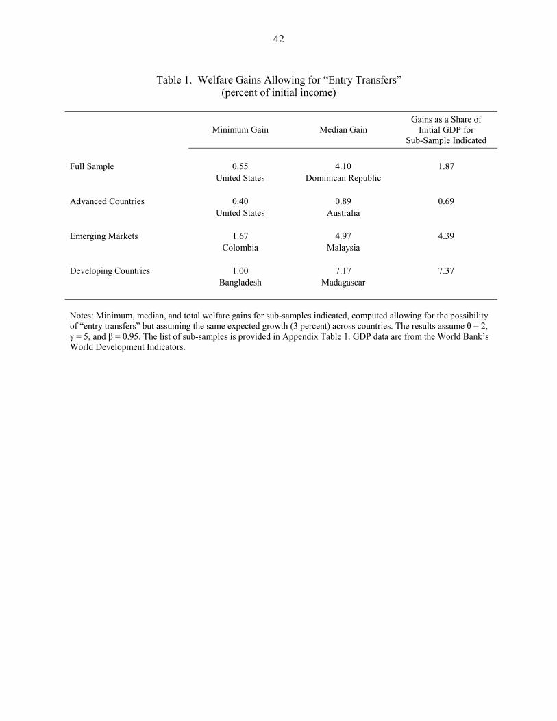
42

Table 1. Welfare Gains Allowing for “Entry Transfers” (percent of initial income)

Minimum Gain Median Gain

Gains as a Share of Initial GDP for

Sub-Sample Indicated Full Sample 0.55 4.10 1.87 United States Dominican Republic Advanced Countries 0.40 0.89 0.69 United States Australia Emerging Markets 1.67 4.97 4.39 Colombia Malaysia Developing Countries 1.00 7.17 7.37 Bangladesh Madagascar Notes: Minimum, median, and total welfare gains for sub-samples indicated, computed allowing for the possibility of “entry transfers” but assuming the same expected growth (3 percent) across countries. The results assume θ = 2, γ = 5, and β = 0.95. The list of sub-samples is provided in Appendix Table 1. GDP data are from the World Bank’s World Development Indicators.

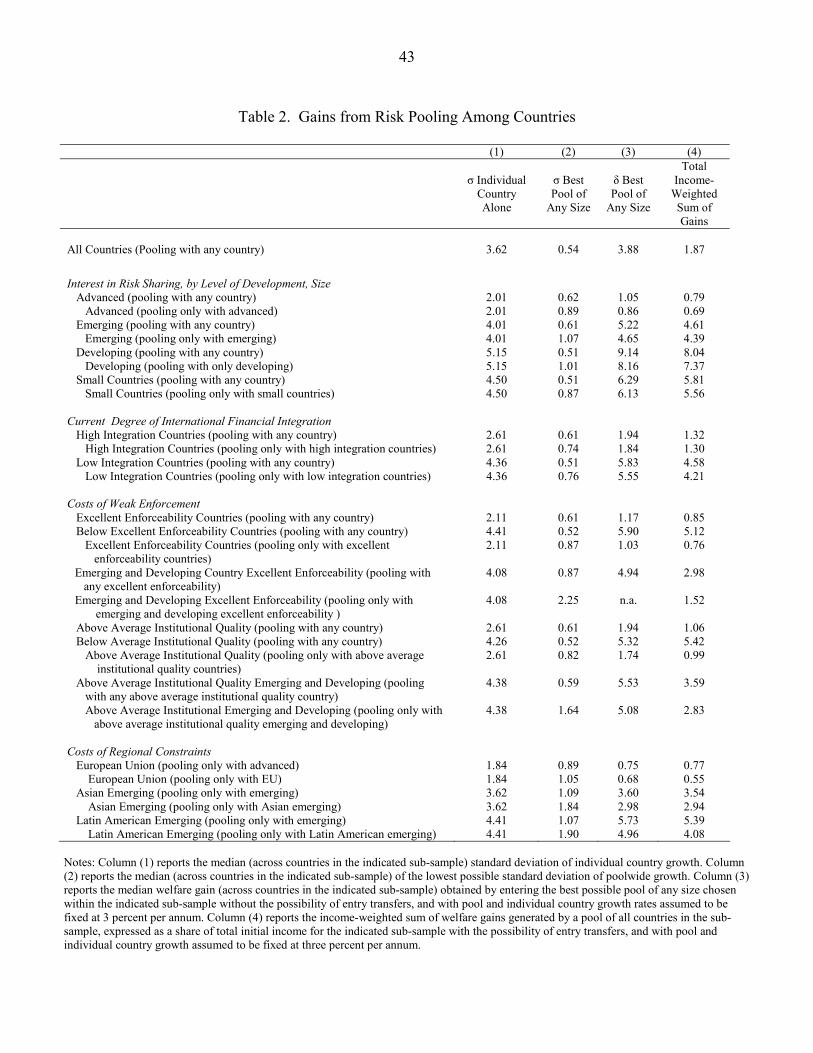
43

Table 2. Gains from Risk Pooling Among Countries

(1) (2) (3) (4)

σ Individual Country Alone

σ Best Pool of

Any Size

δ Best Pool of

Any Size

Total Income-

Weighted Sum of Gains

All Countries (Pooling with any country)

3.62

0.54

3.88

1.87

Interest in Risk Sharing, by Level of Development, Size

Advanced (pooling with any country) 2.01 0.62 1.05 0.79 Advanced (pooling only with advanced) 2.01 0.89 0.86 0.69 Emerging (pooling with any country) 4.01 0.61 5.22 4.61 Emerging (pooling only with emerging) 4.01 1.07 4.65 4.39 Developing (pooling with any country) 5.15 0.51 9.14 8.04 Developing (pooling with only developing) 5.15 1.01 8.16 7.37 Small Countries (pooling with any country) 4.50 0.51 6.29 5.81 Small Countries (pooling only with small countries) 4.50 0.87 6.13 5.56

Current Degree of International Financial Integration High Integration Countries (pooling with any country) 2.61 0.61 1.94 1.32 High Integration Countries (pooling only with high integration countries) 2.61 0.74 1.84 1.30 Low Integration Countries (pooling with any country) 4.36 0.51 5.83 4.58 Low Integration Countries (pooling only with low integration countries) 4.36 0.76 5.55 4.21

Costs of Weak Enforcement Excellent Enforceability Countries (pooling with any country) 2.11 0.61 1.17 0.85 Below Excellent Enforceability Countries (pooling with any country) 4.41 0.52 5.90 5.12 Excellent Enforceability Countries (pooling only with excellent enforceability countries)

2.11 0.87 1.03 0.76

Emerging and Developing Country Excellent Enforceability (pooling with any excellent enforceability)

4.08 0.87 4.94 2.98

Emerging and Developing Excellent Enforceability (pooling only with emerging and developing excellent enforceability )

4.08 2.25 n.a. 1.52

Above Average Institutional Quality (pooling with any country) 2.61 0.61 1.94 1.06 Below Average Institutional Quality (pooling with any country) 4.26 0.52 5.32 5.42 Above Average Institutional Quality (pooling only with above average institutional quality countries)

2.61 0.82 1.74 0.99

Above Average Institutional Quality Emerging and Developing (pooling with any above average institutional quality country)

4.38 0.59 5.53 3.59

Above Average Institutional Emerging and Developing (pooling only with above average institutional quality emerging and developing)

4.38 1.64 5.08 2.83

Costs of Regional Constraints European Union (pooling only with advanced) 1.84 0.89 0.75 0.77 European Union (pooling only with EU) 1.84 1.05 0.68 0.55 Asian Emerging (pooling only with emerging) 3.62 1.09 3.60 3.54 Asian Emerging (pooling only with Asian emerging) 3.62 1.84 2.98 2.94 Latin American Emerging (pooling only with emerging) 4.41 1.07 5.73 5.39 Latin American Emerging (pooling only with Latin American emerging) 4.41 1.90 4.96 4.08

Notes: Column (1) reports the median (across countries in the indicated sub-sample) standard deviation of individual country growth. Column (2) reports the median (across countries in the indicated sub-sample) of the lowest possible standard deviation of poolwide growth. Column (3) reports the median welfare gain (across countries in the indicated sub-sample) obtained by entering the best possible pool of any size chosen within the indicated sub-sample without the possibility of entry transfers, and with pool and individual country growth rates assumed to be fixed at 3 percent per annum. Column (4) reports the income-weighted sum of welfare gains generated by a pool of all countries in the sub-sample, expressed as a share of total initial income for the indicated sub-sample with the possibility of entry transfers, and with pool and individual country growth assumed to be fixed at three percent per annum.

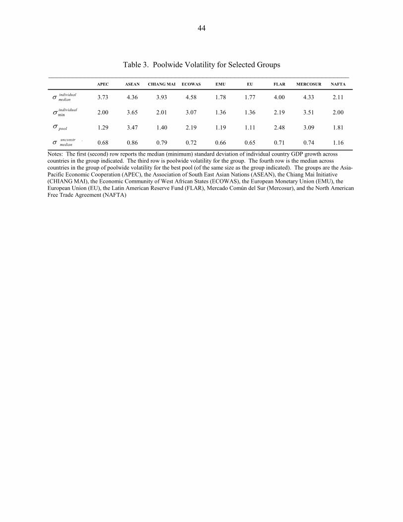
44

Table 3. Poolwide Volatility for Selected Groups

____________________________________________________________________________ APEC ASEAN CHIANG MAI ECOWAS EMU EU FLAR MERCOSUR NAFTA

3.73 4.36 3.93 4.58 1.78 1.77 4.00 4.33 2.11

2.00 3.65 2.01 3.07 1.36 1.36 2.19 3.51 2.00

1.29 3.47 1.40 2.19 1.19 1.11 2.48 3.09 1.81

0.68 0.86 0.79 0.72 0.66 0.65 0.71 0.74 1.16

poolσ

.unconstrmedianσ

individualmedianσ

individualminσ

Notes: The first (second) row reports the median (minimum) standard deviation of individual country GDP growth across countries in the group indicated. The third row is poolwide volatility for the group. The fourth row is the median across countries in the group of poolwide volatility for the best pool (of the same size as the group indicated). The groups are the Asia-Pacific Economic Cooperation (APEC), the Association of South East Asian Nations (ASEAN), the Chiang Mai Initiative (CHIANG MAI), the Economic Community of West African States (ECOWAS), the European Monetary Union (EMU), the European Union (EU), the Latin American Reserve Fund (FLAR), Mercado Común del Sur (Mercosur), and the North American Free Trade Agreement (NAFTA)

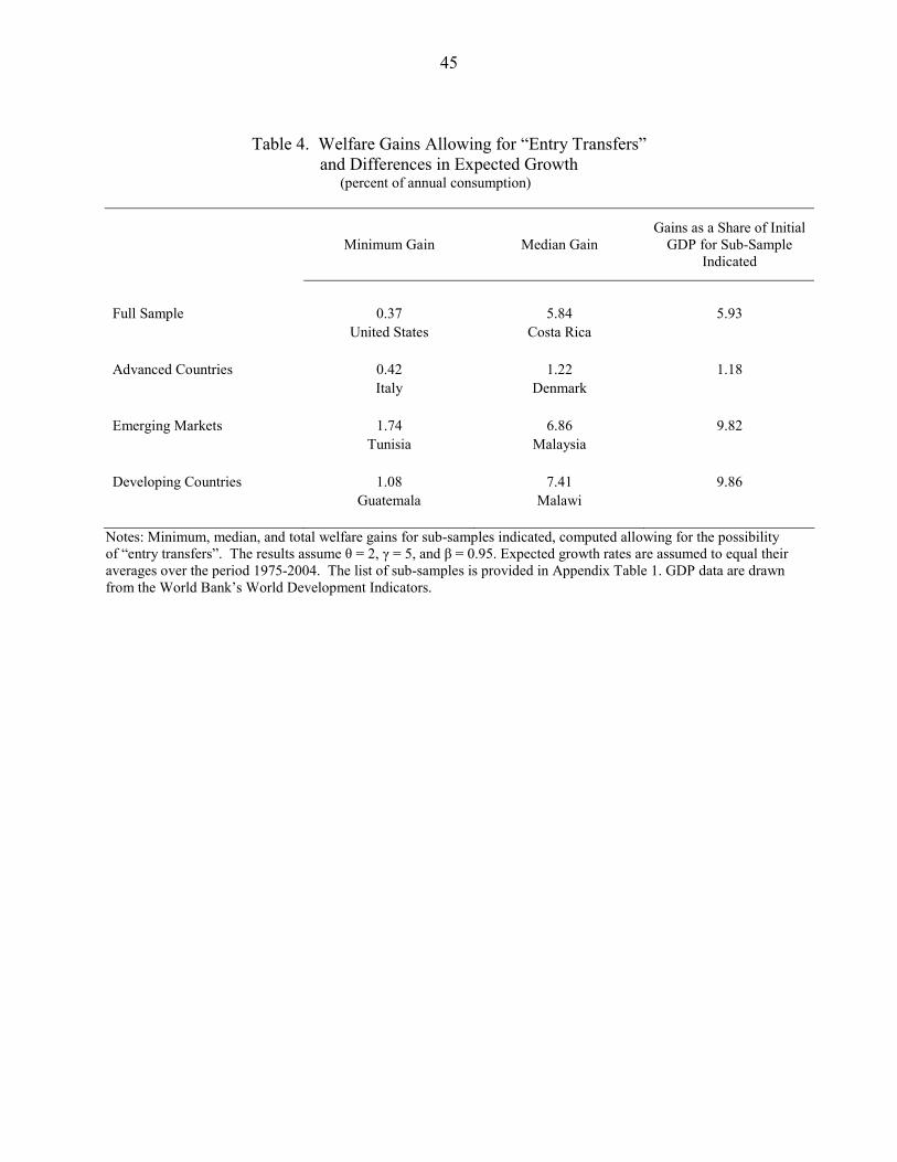
45

Table 4. Welfare Gains Allowing for “Entry Transfers”

and Differences in Expected Growth (percent of annual consumption)

Minimum Gain Median Gain Gains as a Share of Initial

GDP for Sub-Sample Indicated

Full Sample 0.37 5.84 5.93 United States Costa Rica Advanced Countries 0.42 1.22 1.18 Italy Denmark Emerging Markets 1.74 6.86 9.82 Tunisia Malaysia Developing Countries 1.08 7.41 9.86 Guatemala Malawi

Notes: Minimum, median, and total welfare gains for sub-samples indicated, computed allowing for the possibility of “entry transfers”. The results assume θ = 2, γ = 5, and β = 0.95. Expected growth rates are assumed to equal their averages over the period 1975-2004. The list of sub-samples is provided in Appendix Table 1. GDP data are drawn from the World Bank’s World Development Indicators.

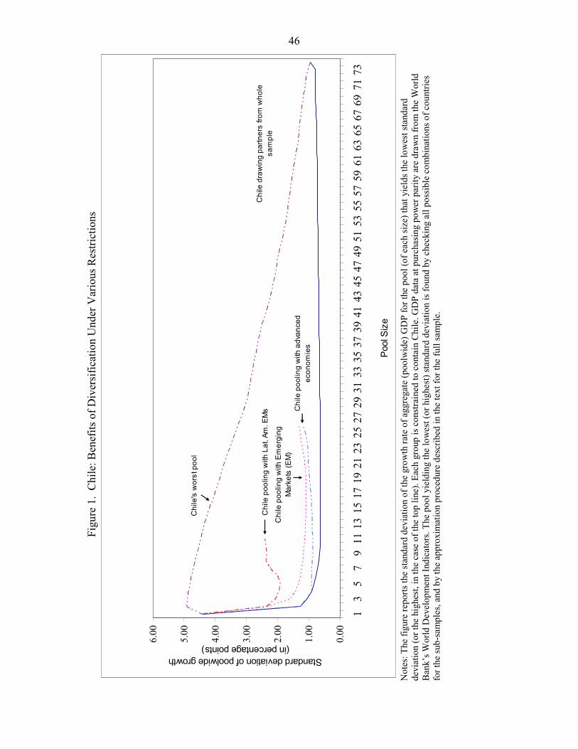
46

Figu

re 1

. C

hile

: Ben

efits

of D

iver

sific

atio

n U

nder

Var

ious

Res

trict

ions

Chi

le d

raw

ing

partn

ers

from

who

le

sam

ple

Chi

le p

oolin

g w

ith E

mer

ging

M

arke

ts (E

M)

Chi

le p

oolin

g w

ith L

at. A

m. E

Ms C

hile

poo

ling

with

adv

ance

d ec

onom

ies

Chi

le's

wor

st p

ool

0.00

1.00

2.00

3.00

4.00

5.00

6.00

13

57

911

1315

1719

2123

2527

2931

3335

3739

4143

4547

4951

5355

5759

6163

6567

6971

73

Poo

l Siz

e

Standard deviation of poolwide growth(in percentage points)

N

otes

: The

figu

re re

ports

the

stan

dard

dev

iatio

n of

the

grow

th ra

te o

f agg

rega

te (p

oolw

ide)

GD

P fo

r the

poo

l (of

eac

h si

ze) t

hat y

ield

s the

low

est s

tand

ard

devi

atio

n (o

r the

hig

hest

, in

the

case

of t

he to

p lin

e). E

ach

grou

p is

con

stra

ined

to c

onta

in C

hile

. GD

P da

ta a

t pur

chas

ing

pow

er p

arity

are

dra

wn

from

the

Wor

ld

Ban

k’s W

orld

Dev

elop

men

t Ind

icat

ors.

The

pool

yie

ldin

g th

e lo

wes

t (or

hig

hest

) sta

ndar

d de

viat

ion

is fo

und

by c

heck

ing

all p

ossi

ble

com

bina

tions

of c

ount

ries

for t

he su

b-sa

mpl

es, a

nd b

y th

e ap

prox

imat

ion

proc

edur

e de

scrib

ed in

the

text

for t

he fu

ll sa

mpl

e.

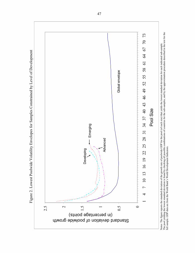
47

Figu

re 2

. Low

est P

oolw

ide

Vol

atili

ty E

nvel

opes

for S

ampl

es C

onst

rain

ed b

y Le

vel o

f Dev

elop

men

t

Glo

bal e

nvel

ope

Adva

nced

Emer

ging

Dev

elop

ing

0

0.51

1.52

2.5

14

710

1316

1922

2528

3134

3740

4346

4952

5558

6164

6770

73

Pool

Size

Standard deviation of poolwide growth (in percentage points)

N

otes

: The

figu

re re

ports

the

stan

dard

dev

iatio

n of

the

grow

th ra

te o

f poo

lwid

e G

DP

for t

he p

ool (

of e

ach

size

) tha

t yie

lds t

he lo

wes

t sta

ndar

d de

viat

ion

for e

ach

indi

cate

d su

b-sa

mpl

e.

The

pool

yie

ldin

g th

e lo

wes

t sta

ndar

d de

viat

ion

is fo

und

by c

heck

ing

all p

ossi

ble

com

bina

tions

of c

ount

ries f

or th

e su

b-sa

mpl

es, a

nd b

y th

e ap

prox

imat

ion

proc

edur

e de

scrib

ed in

the

text

for t

he

full

sam

ple.

GD

P da

ta a

re fr

om th

e W

orld

Ban

k’s W

orld

Dev

elop

men

t Ind

icat

ors.

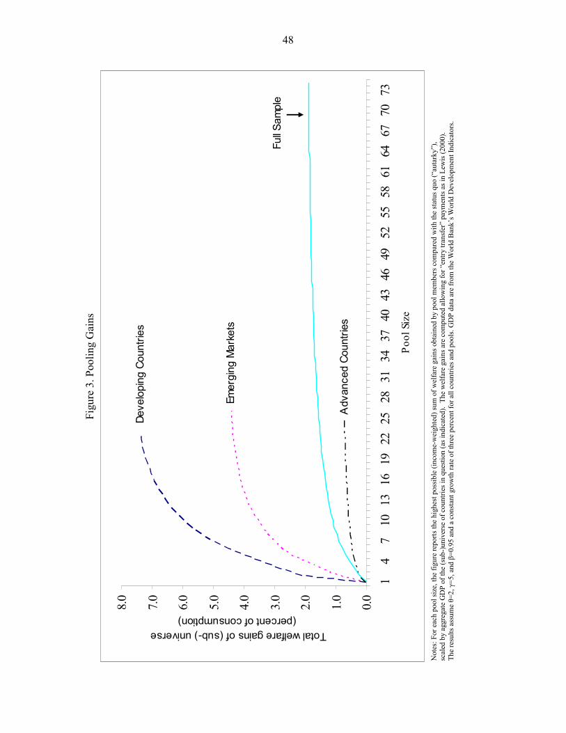
48

Figu

re 3

. Poo

ling

Gai

ns

Deve

lopi

ng C

ount

ries

Emer

ging

Mar

kets

Adv

ance

d Co

untri

es

Full S

ampl

e

0.0

1.0

2.0

3.0

4.0

5.0

6.0

7.0

8.0

14

710

1316

1922

2528

3134

3740

4346

4952

5558

6164

6770

73Po

ol S

ize

Total welfare gains of (sub-) universe(percent of consumption)

N

otes

: For

eac

h po

ol si

ze, t

he fi

gure

repo

rts th

e hi

ghes

t pos

sibl

e (in

com

e-w

eigh

ted)

sum

of w

elfa

re g

ains

obt

aine

d by

poo

l mem

bers

com

pare

d w

ith th

e st

atus

quo

(“au

tark

y”),

scal

ed b

y ag

greg

ate

GD

P of

the

(sub

-)uni

vers

e of

cou

ntrie

s in

ques

tion

(as i

ndic

ated

). T

he w

elfa

re g

ains

are

com

pute

d al

low

ing

for “

entry

tran

sfer

” pa

ymen

ts a

s in

Lew

is (2

000)

.

The

resu

lts a

ssum

e θ=

2, γ

=5, a

nd β

=0.9

5 an

d a

cons

tant

gro

wth

rate

of t

hree

per

cent

for a

ll co

untri

es a

nd p

ools

. GD

P da

ta a

re fr

om th

e W

orld

Ban

k’s W

orld

Dev

elop

men

t Ind

icat

ors.

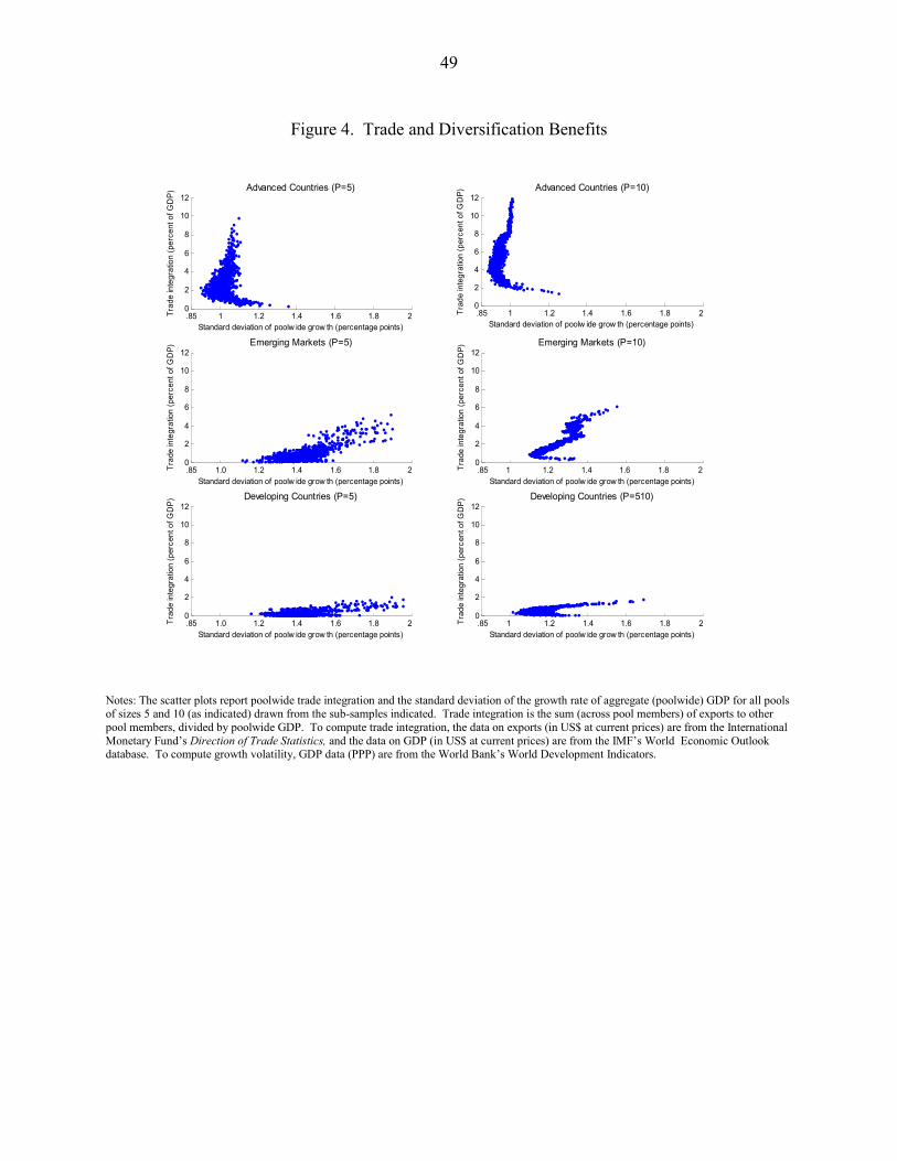
49

Figure 4. Trade and Diversification Benefits

.85 1 1.2 1.4 1.6 1.8 2 0

2

4

6

8

10

12

Standard deviation of poolw ide grow th (percentage points)

Trad

e in

tegr

atio

n (p

erce

nt o

f GD

P)

Advanced Countries (P=5)

.85 1 1.2 1.4 1.6 1.8 2 0

2

4

6

8

10

12

Standard deviation of poolw ide grow th (percentage points)

Trad

e in

tegr

atio

n (p

erce

nt o

f GD

P)

Advanced Countries (P=10)

.85 1 1.2 1.4 1.6 1.8 2 0

2

4

6

8

10

12

Standard deviation of poolw ide grow th (percentage points)

Trad

e in

tegr

atio

n (p

erce

nt o

f GD

P)

Emerging Markets (P=10)

.85 1 1.2 1.4 1.6 1.8 2 0

2

4

6

8

10

12

Standard deviation of poolw ide grow th (percentage points)

Trad

e in

tegr

atio

n (p

erce

nt o

f GD

P)

Developing Countries (P=510)

.85 1.0 1.2 1.4 1.6 1.8 2 0

2

4

6

8

10

12

Standard deviation of poolw ide grow th (percentage points)

Trad

e in

tegr

atio

n (p

erce

nt o

f GD

P)

Emerging Markets (P=5)

.85 1.0 1.2 1.4 1.6 1.8 2 0

2

4

6

8

10

12

Standard deviation of poolw ide grow th (percentage points)

Trad

e in

tegr

atio

n (p

erce

nt o

f GD

P)

Developing Countries (P=5)

Notes: The scatter plots report poolwide trade integration and the standard deviation of the growth rate of aggregate (poolwide) GDP for all pools of sizes 5 and 10 (as indicated) drawn from the sub-samples indicated. Trade integration is the sum (across pool members) of exports to other pool members, divided by poolwide GDP. To compute trade integration, the data on exports (in US$ at current prices) are from the International Monetary Fund’s Direction of Trade Statistics, and the data on GDP (in US$ at current prices) are from the IMF’s World Economic Outlook database. To compute growth volatility, GDP data (PPP) are from the World Bank’s World Development Indicators.

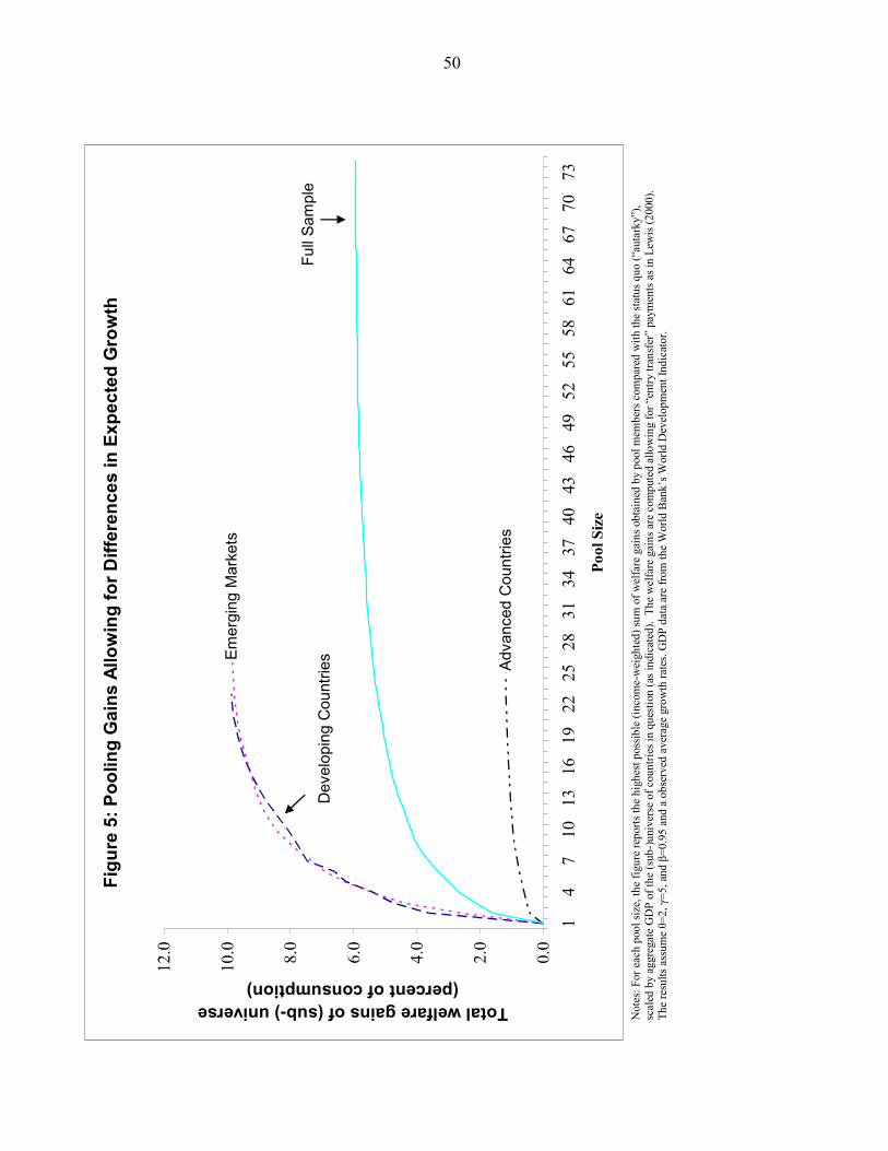
50

Figu

re 5

: Poo

ling

Gai

ns A

llow

ing

for D

iffer

ence

s in

Exp

ecte

d G

row

th

Dev

elop

ing

Cou

ntrie

sEm

ergi

ng M

arke

ts

Adv

ance

d C

ount

ries

Full

Sam

ple

0.0

2.0

4.0

6.0

8.0

10.0

12.0

14

710

1316

1922

2528

3134

3740

4346

4952

5558

6164

6770

73Po

ol S

ize

Total welfare gains of (sub-) universe (percent of consumption)

N

otes

: For

eac

h po

ol si

ze, t

he fi

gure

repo

rts th

e hi

ghes

t pos

sibl

e (in

com

e-w

eigh

ted)

sum

of w

elfa

re g

ains

obt

aine

d by

poo

l mem

bers

com

pare

d w

ith th

e st

atus

quo

(“au

tark

y”),

scal

ed b

y ag

greg

ate

GD

P of

the

(sub

-)uni

vers

e of

cou

ntrie

s in

ques

tion

(as i

ndic

ated

). T

he w

elfa

re g

ains

are

com

pute

d al

low

ing

for “

entry

tran

sfer

” pa

ymen

ts a

s in

Lew

is (2

000)

.

The

resu

lts a

ssum

e θ=

2, γ

=5, a

nd β

=0.9

5 an

d a

obse

rved

ave

rage

gro

wth

rate

s. G

DP

data

are

from

the

Wor

ld B

ank’

s Wor

ld D

evel

opm

ent I

ndic

ator

.