Is Transshipment a Behaviorally-Robust Risk-Pooling Strategy?∗

AJ A. Bostian Charles A. Holt Sanjay Jain Kamalini Ramdas

September 1, 2012

Abstract

Transshipment allows firms with excess supply to sell their inventory directly to firms with excessdemand. Profits should increase with transshipment in place, but behavioral bias could nullify thisimprovement. We extend the newsvendor experiment to accommodate transshipment, and run itwith undergraduate and MBA cohorts. Aggregate ordering patterns mask the true degree of biasin individual decisions. We instead structurally model subjects as adaptive and forward-thinkingdecision makers. Estimates of a mixture model indicate that only about 5 percent of subjectsin either group can be described as forward thinking, while 95 percent appear to be adaptivedecision makers with substantial biases. Individual estimates suggest a wide heterogeneity in biasesand no systematic differences between the subject groups, despite the MBAs’ greater professionalexperience. A key advantage of structural estimation is the ability to undertake a counterfactualexercise to determine how biased subjects would have behaved in the absence of transshipment.Transshipment yields an even greater benefit in the presence of behavioral biases than in the absenceof these biases, making it a behaviorally-robust risk-pooling strategy.

Keywords: transshipment, risk pooling, newsvendor experiment, behavioral bias, experience-weightedattraction, cognitive hierarchy, behavioral heterogeneity, MBA students, undergraduate students

1 Introduction

Transshipment is a risk-pooling technique employed within multi-location supply chains to smooth

out local variations in demand. Firms in a transshipment relationship ship goods directly to each

other to make up for local stock-outs. If one firm stocks out, it can purchase residual supply from its

transshipment partners instead of placing a new order with a supplier.

Rudi et al. (2001) assess the theoretical efficiency of this arrangement in a two-retailer newsvendor

setting in which firms transship between themselves after observing demands. Their analysis generates

two main predictions. First, the profit-maximizing order quantity increases with the transshipment

price τ paid by the firm receiving the transshipment. The intuition for this result can be illustrated by

considering the case of a high τ relative to the wholesale cost. A firm can make large transshipment∗Bostian and Holt: Department of Economics, University of Virginia, Charlottesville, VA 22904-4182 USA. Jain: Fac-

ulty of Economics, University of Cambridge, Cambridge CB3 9DD UK. Ramdas: Management Science and Operations,London Business School, London NW1 4SA UK. This research was supported in part by the National Science Foundation(SES-0098400). We thank Nitin Bakshi, Woonam Hwang, and Serguei Netessine for helpful comments. We also thankCourtney Mallow for her valuable laboratory assistance.

1

profits by sending units to its partner, but it will lose (in opportunity-cost terms) if it receives a

transshipment because of the higher price it must pay for the good. Ordering a larger quantity

lessens the probability of receiving a low-profit transshipment, and also increases the likelihood of

having stock on hand to transship out at a profit. Because the partner firm faces identical incentives,

equilibrium orders are set so that neither firm can systematically take advantage of the other through

the transshipment arrangement. The second and more interesting result from a risk-management

perspective is that expected profits are higher with transshipment in place than without.1

While these theoretical results are promising, achieving this beneficial equilibrium requires man-

agers to correctly interpret transshipment incentives. Managerial behavior can sometimes deviate

from optimal predictions, underscoring a potential disconnect between theoretical and actual decision-

making processes (see Bendoly et al., 2006; Gans and Croson, 2008; Gino and Pisano, 2008). In

particular, behavioral biases may drive managers away from a profit-maximizing outcome. However,

empirically testing if managers are actually susceptible to behavioral bias can be difficult, because it is

hard to find data that can disentangle a behavioral effect from other relevant but confounding factors

affecting managerial decisions.

Laboratory experiments have thus provided many of the empirical insights about potential bias in

a managerial context. Experiments on the newsvendor setting in particular (see Croson and Donohue,

2002) have established a “pull-to-center” effect, in which orders cluster around the center of the demand

distribution instead of around the optimum (see Bearden et al., 2008; Bolton and Katok, 2008; Bostian

et al., 2008; Lurie and Swaminathan, 2009; Schweitzer and Cachon, 2000). They have also found a

“bullwhip” effect in multi-level supply chains (see Croson and Donohue, 2006; Croson et al., 2005),

by which order imbalances are magnified up the chain. Differences in these effects have also been

associated with risk attitudes and gender (de Véricourt et al., 2011). The fact that these non-optimal

outcomes have been observed in a controlled laboratory setting strongly suggests that they stem from

behavioral bias, not job-specific factors.

Transshipment substantially complicates the newsvendor problem, providing more channels through

which bias can work. In addition to local market incentives, each firm now has an additional strategic

motive to set its orders to avoid or to solicit transshipments (depending on which side of the transaction

is more profitable). A profit-maximizing equilibrium involves balancing of these motives, attaining the

beneficial aspects of transshipment. However, if managers possess behavioral biases that lead to an

incorrect assessment of these strategic incentives, the benefits from transshipment may be eliminated.1Dong and Rudi (2004) and Zhang (2005) additionally examine the effects of upstream pricing power in the transship-

ment arrangement, and Dong and Rudi (2004) and Hu et al. (2007) examine the conditions under which the transshipmentprice induces globally-optimal orders across a supply chain.

2

To study managerial decision making in a transshipment setting, we replicate the Rudi et al. (2001)

model in an incentivized experiment. Of course, questions of external validity are almost guaranteed to

arise when generalizing laboratory results to a broader group, such as managers. One way to assess the

relevance of “manager” characteristics in an experiment is to compare decisions by “manager-like” people

with professional experience, to those by “non-manager-like” people who lack professional experience.2

We magnify the potential effect of manager characteristics in this study by comparing two groups

with widely disparate professional experiences: undergraduate and MBA students at the University of

Virginia. The average undergraduate student in this group has almost no work experience, while the

average MBA student has about five years of work experience and has been exposed to the newsvendor

framework.3 4

The treatment variable in our experiment is the transshipment price τ , which we set above and

below the wholesale price in different treatments. This results in theoretical equilibria above and below

the center of the demand distribution. We match subjects with the same partner for two 15-round

treatments to allow decision heuristics to stabilize. We find that median orders do increase in τ , but

are also pulled towards the center of the demand distribution. Importantly, a closer inspection of the

data indicates that these aggregate measures mask substantial individual variation. A reduced-form

regression further shows that an average subject’s decisions are strongly affected by his or her own

outcome history.

Building on this reduced-form analysis, we structurally model decision-making behavior to examine

the behavioral robustness of transshipment. A key advantage of the structural approach is the ability to

construct counterfactuals, and we are particularly interested in determining whether the transshipment

arrangement has improved our subjects’ profits. In these structural models, we consider two polar-

opposite assumptions about the nature of learning. By modifying the adaptive experience-weighted

attraction (EWA) model (Camerer and Ho, 1999), we first consider learning as a purely empirical

exercise of examining which decisions have worked well in the past. EWA agents are purely adaptive

learners, and can possess four biases affecting their interpretation of historical data: recency (a tendency

to focus on more recent events), reinforcement (a tendency to ignore counterfactual outcomes), lock-2Fréchette (forthcoming) surveys experimental research that uses both professionals and students, finding conflicting

evidence on whether professionals systematically perform better than students. It thus seems that the empirical questionof whether professionals or students are more likely to exhibit behavioral bias in the laboratory is open. In a study ofsingle-retailer newsvendor decisions, Bolton et al. (forthcoming) find that undergraduates, graduates, and professionalsall exhibit the pull-to-center effect. Our study similarly finds bias in both undergraduates and MBAs, but we additionallyidentify behavioral sources of these biases.

3We thank the MBA Admissions Office and the Office of Institutional Assessment and Studies at the University ofVirginia for providing these summary statistics.

4One could question whether factors other than professional experience (e.g., maturity) might also explain any dis-parities in these two groups. Because we do not ultimately find any substantive differences between undergraduates andMBAs, we believe that such factors are not playing a major role in this experiment.

3

on (a tendency to settle quickly on a strategy), and inattention (a tendency to ignore information

coming from a partner). Next, we consider learning as a purely introspective exercise of determining

the optimal order quantity given the game’s incentives, using the forward-thinking cognitive hierarchy

(CH) model (Camerer et al. 2004). Bias arises in a CH agent because he or she stops a mental

best-response calculation before reaching the theoretical optimum.

We can make much more precise statements about the nature of bias with these structural models

than are possible through reduced-form approaches.5 For example, when we allow the data to determine

the mixture of learning types, we find that the most empirically-plausible explanation is that subjects

are adaptive learners. An overwhelming 96% of undergraduates and 98% of MBAs are best described

as adaptive, with substantial biases in interpreting historical outcomes. The remaining subjects best

fit the forward-thinking model, engaging in about four steps of mental best response. Their orders

are fairly close to the profit-maximizing order, and they use this approximate strategy throughout

the experiment. The forward thinkers in the MBA group appear to think about a half step further

than those in the undergraduate group, a difference that yields only a minimal increase in predicted

profits. Because the vast majority of subjects are adaptive learners, we use the EWA-style model when

formulating counterfactuals.

To construct a counterfactual tailored to each subject, we also examine bias at the individual level

by estimating EWA and CH bias parameters for each subject. Far from being clustered around the

cohort-level point estimates (as might be inferred from their tight standard errors), individual EWA

estimates span most of the parameter space. An important finding is that the bias profile of subjects

in the MBA cohort is not that much different from that of the undergraduate cohort. The subjects in

both groups range from very rational to very biased.

Finally, we use these individual estimates to construct a no-transshipment counterfactual for each

subject, which allows us to assess the merits of transshipment in the context of decision bias. When

orders are so clearly suboptimal, and subjects are biased in such disparate ways, it is reasonable to

ask whether transshipment has any efficacy at all. The adaptive decision predictions with and without

transshipment show that transshipment has improved the profitability of each and every subject. Most

interestingly, transshipment has an even stronger benefit in the presence of biases than in their absence.

For the median subject, the counterfactual percentage improvement in profit with the transshipment

arrangement in place exceeds the theoretical improvement by a quarter to almost a half. Transshipment5The structural method has been applied in other newsvendor experiments to tease out substantive behavioral patterns

from noisy data. For example, Bostian et al. (2008) use an abbreviated EWA model to assess learning biases in a single-retailer newsvendor design. In an evaluation of increasingly complex price offerings by a supplier, Kalkanci et al. (2011)use the same model to find that the rules of thumb implemented in more complex situations generally involve greaterbias. In a centrally-controlled multi-retailer design, Ho et al. (2010) estimate a utility specification in which stock-outsgenerate greater psychological upheaval than understocks.

4

thus appears to be a “behaviorally-robust” risk-management tool. In other words, the benefits from

transshipment accrue even in the presence of behavioral biases. This aspect of its usefulness that has

not been previously considered.

2 Theoretical Setup

Our experiment is based on a simple newsvendor model with two firms, each operating independently

in a separate market for the same good.6 A uniform retail price p and marginal wholesale cost c prevail

in each market. Demand in each market is random, and the two firms do not know their local demands

when placing orders. The firms are in an exclusive and enforceable transshipment relationship, so that

ex post demand imbalances are rectified whenever possible by shipping goods from the firm with excess

supply to the firm facing excess demand. Each unit transshipped involves a price τ ≤ p, paid by the

firm receiving the transshipped goods to the firm making the transshipment.

Let x1 and x2 denote the uncertain demands faced by Firms 1 and 2, and let q1 and q2 denote

their respective order quantities. Let F denote the joint demand distribution, which has lower bounds

a1 and a2 and upper bounds b1 and b2. Given Firm 2’s order q2, the expected profit to Firm 1 from

ordering q1 is

E [π1 (q1|q2)] =

ˆ q1

a1

ˆ q2

a2

(px1 − cq1) dF (x1, x2) +

ˆ b1

q1

ˆ b2

q2

(pq1 − cq1) dF (x1, x2)

+

ˆ q1

a1

ˆ b2

q2

(px1 − cq1 + τ min {q1 − x1, x2 − q2}) dF (x1, x2)

+

ˆ b1

q1

ˆ q2

a2

(pq1 − cq1 + (p− τ) min {x1 − q1, q2 − x2}) dF (x1, x2)

The four integrals in this equation reflect the four possible market outcomes. In the first, both firms

have excess supply, and each locally sells a quantity equal to its own demand. In the second, both firms

have excess demand, and each locally sells the quantity it ordered. In the third, Firm 1 has excess

supply, and Firm 2 has excess demand. Here, Firm 1 locally sells its own demand quantity, and ships

to Firm 2 the smaller of Firm 1’s excess supply, or Firm 2’s excess demand. Firm 2 pays τ to Firm 1

for each transshipped unit, and locally sells these units for p. The fourth outcome is identical to the

third, with the roles of Firm 1 and Firm 2 reversed.6We use the term “market” as shorthand for the incentive structure corresponding to a transshipment arrangement,

and “firm” as shorthand for a decision maker who faces these incentives. Under this reading, a firm can represent anowner of an independent company, a manager of a unit within a larger company, or a subject in our experiment.

5

In our experiment, x1 and x2 are i.i.d. uniform variables, leading to a simplified expression:7

E [π1 (q1|q2)] = p · 1

b− a

ˆ q1

ax1dx1 + p · 1

b− aq1

ˆ b

q1

dx1 − cq1

+ τ · 1

(b− a)2

ˆ q1

a

[ˆ b

q2

min {q1 − x1, x2 − q2} dx2

]dx1

+ (p− τ) · 1

(b− a)2

ˆ b

q1

[ˆ q2

amin {x1 − q1, q2 − x2} dx2

]dx1 (1)

The optimality condition for (1) is8

∂E [π1 (q1|q2)]

∂q1= 0 ⇒ p · 1

b− a(b− q1) (2)

+τ · 1

(b− a)2

[(b− q2 − q1) (q1 − a) +

1

2

(q2

1 − a2)]

+ (p− τ) · 1

(b− a)2

[(a− q2 − q1) (b− q1) +

1

2

(b2 − q2

1

)]= c

The first line in (2) is the expected marginal revenue from ordering a unit and selling it locally. (This is

the marginal revenue without a transshipment arrangement in place.) The second line is the expected

marginal revenue from ordering a unit and transshipping it to Firm 2, while the third line is the

expected marginal revenue from foregoing a marginal order and instead selling a unit that has been

transshipped from Firm 2. In equilibrium, the sum of these three expected-revenue streams must equal

the marginal cost of production.

Equation (2) is quadratic in q1, and the roots of this quadratic define a complicated best-response

function q1 (q2). In the left panel of Figure 1, we plot the four functions corresponding to our experi-

mental setup: p = $0.40, c = $0.20, a = 0, b = 200, and treatment variables of τ = $0.00, $0.10, $0.30,

and $0.40. The function q1 (q2) shifts out uniformly as τ increases, implying that a high transshipment

price leads Firm 1 to increase its order in the hope of transshipping excess supply to Firm 2. Also,

q1 (q2) is concave when τ is lower than p, and convex when higher than p. To see the intuition for this

result, consider first the former case (corresponding to τ = $0.00 and $0.10). Here, Firm 1 should re-

duce its order quantity as q2 rises for two reasons: the likelihood of transshipping out falls with q2, and

only the incoming transshipments are profitable. In the latter case (corresponding to τ = $0.30 and

$0.40), an increase in q2 again causes the likelihood of transshipping out to fall, but now transshipping

out is profitable, causing q1 to fall relatively slowly.7See Rudi et al. (2001) and Dong and Rudi (2004) for theoretical treatments of related problems involving transship-

ment.8The derivation is made easier by noting that min {q1 − x1, x2 − q2} and min {x1 − q1, q2 − x2} define trapezoidal

areas over their respective ranges of integration.

6

The right panel of Figure 1 plots the optimal order quantity q? for the four values of τ , as well as

the expected transshipment quantity received. When τ is low, both firms restrict their local orders in

an attempt to receive inexpensive transshipments. The opposite effect occurs when τ is high. However,

the equilibrium transshipment quantity is essentially 0 in each case, implying that neither firm can

systematically take advantage of the other via the transshipment arrangement. On average, each firm

will receive about as many transshipped units as it sends.

Table 1 provides the optimal order quantities and expected profits for the four experimental treat-

ments. Without transshipment, the optimal order quantity would be 100 units, and the expected

profit would be $10.00. The optimal order falls below 100 units when p − τ > τ , and rises above it

when p − τ < τ . The optimal expected profit with transshipment is about 30% higher than without

transshipment for all four values of τ .

3 Experimental Design

We recruited an undergraduate cohort and an MBA cohort from the University of Virginia. The

undergraduate cohort came from the standing subject pool at the Veconlab Experimental Economics

Laboratory, which consists mostly of economics and business majors. The MBA cohort was recruited

from the Darden Graduate School of Business. The MBA students had completed their first or second

years of the MBA program, and had been exposed to the newsvendor framework.

Each subject was anonymously matched with the same partner for 30 repetitions of the two-

firm newsvendor game outlined above. The first 15 rounds were played under one τ treatment; an

unannounced treatment change was then made at the start of round 16, effective for the remaining 15

rounds. This treatment change was symmetric about the wholesale cost c (i.e., |τ1 − c| = |c− τ2| for

the two transshipment prices τ1 and τ2), which implied symmetry in q? about the center of the demand

distribution (q = 100). Thus, subjects were exposed to “mirror image” transshipment incentives in each

of the 15-round blocks.

Table 2 summarizes our sessions. At least 12 subjects from each cohort participated in each session,

with the participant numbers within a treatment equally balanced across cohorts. We conducted the

experiment using the “Supply Chain” program in the Veconlab suite of web-based economics experi-

ments.9 At the start of a session, we paid subjects USD 10 for on-time arrival, and seated them at

blinded computer stations. We began the experiment by reading the instructions aloud while subjects

followed along with an identical version printed on-screen. The Veconlab program then assigned anony-

mous fixed pairings to the subjects, and each pair played two 15-round treatments of the newsvendor9Instructions can be found on the Veconlab website: http://veconlab.econ.virginia.edu/sc/sc.php.

7

game with transshipments. We did not reveal the number of rounds in the session, or the fact that a

treatment change would be made midway. At the end of the session, we paid subjects in cash according

to the amount they had earned, using a conversion rate of $20.00 to USD 1.10

Each subject began a round of the experiment by choosing an order quantity. After the subject’s

partner had also chosen an order quantity, the program randomly drew demand quantities for the two

local markets, and automatically transshipped units when feasible.11 Critically, a subject could not

observe the partner’s order quantity or demand quantity, only the quantity transshipped into or out

of the local market. At the end of each round, subjects reviewed their own costs and revenues, their

transshipment prices and revenues, and decision history. Subjects proceeded through all 30 rounds at

their own natural paces, and each session lasted about one hour.

4 Aggregate Patterns and Reduced-Form Results

For greatest statistical efficiency, our analysis makes use of the full 30-round decision profile for each

subject. Of course, a treatment change could induce a sequence effect in these decisions, because

subjects may not have immediately adjusted to the new incentives. Such a sequence effect could bias

our analysis. However, because the two treatments had mirror-image incentives, subjects may also

have quickly inverted their decision heuristics for the second treatment. The intensity of the sequence

effect is thus an empirical question.

A simple way to eliminate the possibility of a sequencing bias is to discard the last half of the data

from each session. Of course, eliminating data sacrifices statistical precision. We instead design our

reduced-form and structural models with econometric controls for the potential sequence effect, and

use all 30 rounds of data. We also report the 30-round values of aggregate descriptive statistics (e.g.,

order quantities and profits). We usually find that these statistics and associated hypothesis tests are

not meaningfully different (in statistical or economic terms) when using the 15- or 30-round estimates.

For the interested reader, we provide 15-round analogs to each test and model in the online appendix.

4.1 Aggregate Patterns

Table 3 provides the median profits for the two cohorts, both in five-round windows and overall.12

None of the cohort differences are statistically significant in any treatment using the Mann-Whitney U

test, either in five-round windows or overall. Median profits are 3% to 15% lower than the theoretical10Dollar amounts ($) refer to experimental currency amounts, not cash payments.11Each demand sequence was assigned to one undergraduate subject and one MBA subject.12We prefer the median as the measure of central tendency because it can provide a better view of central tendency in

small samples with one or two outliers. Aggregate measures with either 12 or 14 data points are particularly susceptibleto outlier effects.

8

optimum, suggesting the presence of suboptimal orders. However, the median profit is greater than

would be theoretically expected without transshipment ($150.00), previewing our finding that trans-

shipment improves profits even if subjects may have had some difficulty with the decision problem.

A profit trend is also apparent window-by-window: profits tend to be highest in the first five rounds,

falling (sometimes quite sharply) in the second five-round interval, and rebounding moderately in the

third (though the downward trend continues in a handful of cases). This cyclicality is also a first

indication of adaptivity.

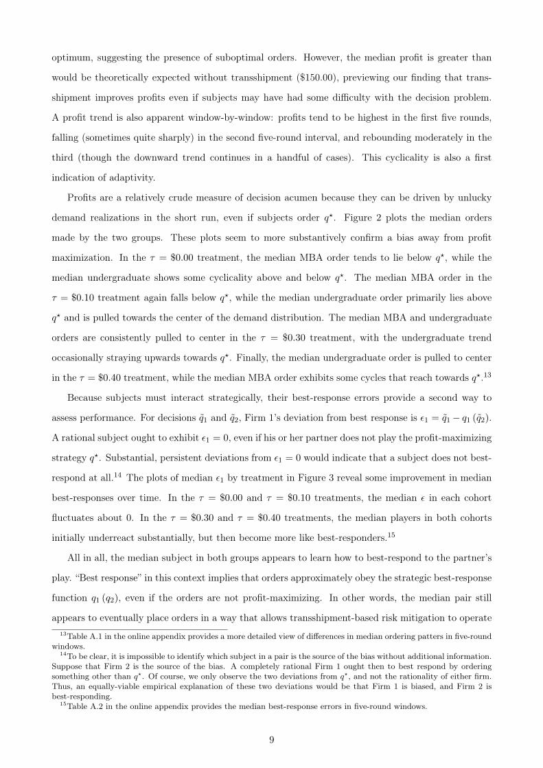
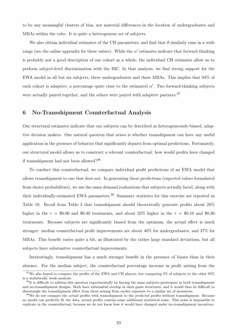
Profits are a relatively crude measure of decision acumen because they can be driven by unlucky

demand realizations in the short run, even if subjects order q?. Figure 2 plots the median orders

made by the two groups. These plots seem to more substantively confirm a bias away from profit

maximization. In the τ = $0.00 treatment, the median MBA order tends to lie below q?, while the

median undergraduate shows some cyclicality above and below q?. The median MBA order in the

τ = $0.10 treatment again falls below q?, while the median undergraduate order primarily lies above

q? and is pulled towards the center of the demand distribution. The median MBA and undergraduate

orders are consistently pulled to center in the τ = $0.30 treatment, with the undergraduate trend

occasionally straying upwards towards q?. Finally, the median undergraduate order is pulled to center

in the τ = $0.40 treatment, while the median MBA order exhibits some cycles that reach towards q?.13

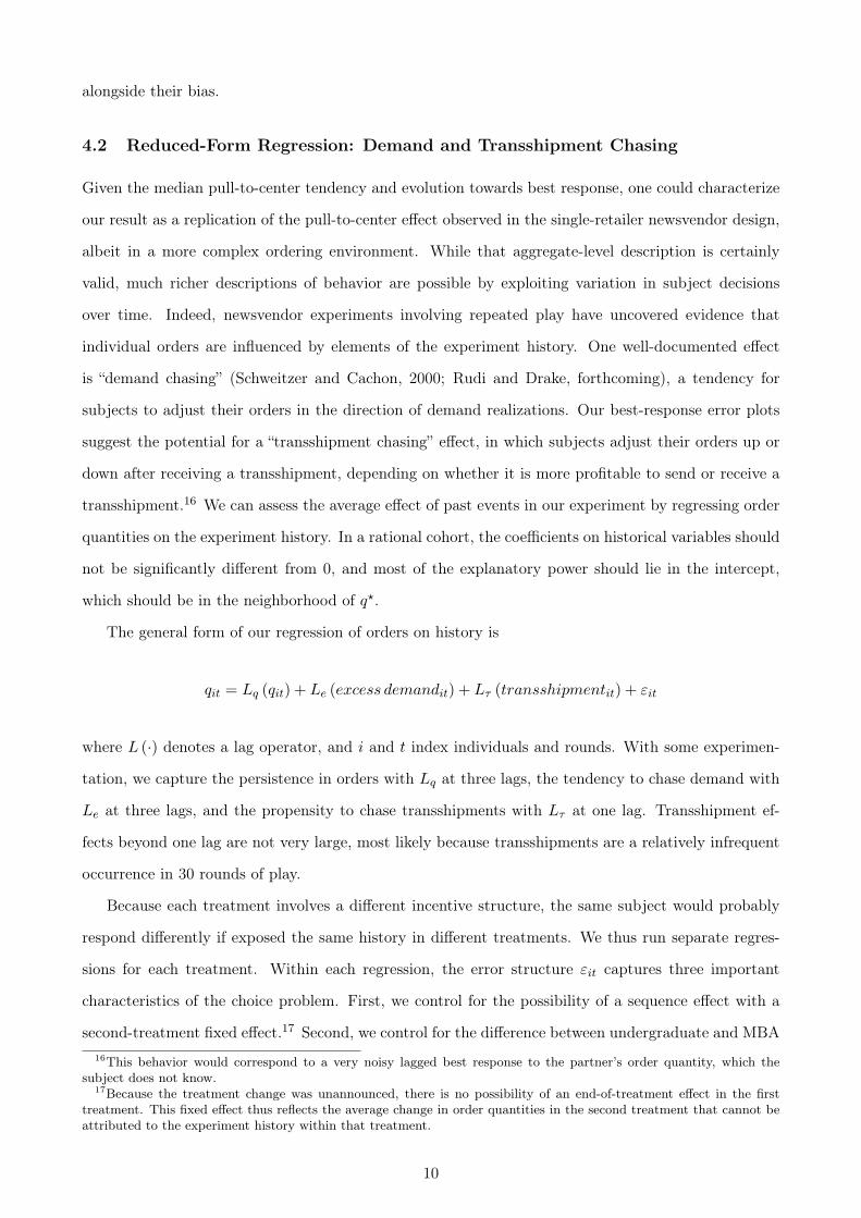
Because subjects must interact strategically, their best-response errors provide a second way to

assess performance. For decisions q1 and q2, Firm 1’s deviation from best response is ε1 = q1− q1 (q2).

A rational subject ought to exhibit ε1 = 0, even if his or her partner does not play the profit-maximizing

strategy q?. Substantial, persistent deviations from ε1 = 0 would indicate that a subject does not best-

respond at all.14 The plots of median ε1 by treatment in Figure 3 reveal some improvement in median

best-responses over time. In the τ = $0.00 and τ = $0.10 treatments, the median ε in each cohort

fluctuates about 0. In the τ = $0.30 and τ = $0.40 treatments, the median players in both cohorts

initially underreact substantially, but then become more like best-responders.15

All in all, the median subject in both groups appears to learn how to best-respond to the partner’s

play. “Best response” in this context implies that orders approximately obey the strategic best-response

function q1 (q2), even if the orders are not profit-maximizing. In other words, the median pair still

appears to eventually place orders in a way that allows transshipment-based risk mitigation to operate13Table A.1 in the online appendix provides a more detailed view of differences in median ordering patters in five-round

windows.14To be clear, it is impossible to identify which subject in a pair is the source of the bias without additional information.

Suppose that Firm 2 is the source of the bias. A completely rational Firm 1 ought then to best respond by orderingsomething other than q?. Of course, we only observe the two deviations from q?, and not the rationality of either firm.Thus, an equally-viable empirical explanation of these two deviations would be that Firm 1 is biased, and Firm 2 isbest-responding.

15Table A.2 in the online appendix provides the median best-response errors in five-round windows.

9

alongside their bias.

4.2 Reduced-Form Regression: Demand and Transshipment Chasing

Given the median pull-to-center tendency and evolution towards best response, one could characterize

our result as a replication of the pull-to-center effect observed in the single-retailer newsvendor design,

albeit in a more complex ordering environment. While that aggregate-level description is certainly

valid, much richer descriptions of behavior are possible by exploiting variation in subject decisions

over time. Indeed, newsvendor experiments involving repeated play have uncovered evidence that

individual orders are influenced by elements of the experiment history. One well-documented effect

is “demand chasing” (Schweitzer and Cachon, 2000; Rudi and Drake, forthcoming), a tendency for

subjects to adjust their orders in the direction of demand realizations. Our best-response error plots

suggest the potential for a “transshipment chasing” effect, in which subjects adjust their orders up or

down after receiving a transshipment, depending on whether it is more profitable to send or receive a

transshipment.16 We can assess the average effect of past events in our experiment by regressing order

quantities on the experiment history. In a rational cohort, the coefficients on historical variables should

not be significantly different from 0, and most of the explanatory power should lie in the intercept,

which should be in the neighborhood of q?.

The general form of our regression of orders on history is

qit = Lq (qit) + Le (excess demandit) + Lτ (transshipmentit) + εit

where L (·) denotes a lag operator, and i and t index individuals and rounds. With some experimen-

tation, we capture the persistence in orders with Lq at three lags, the tendency to chase demand with

Le at three lags, and the propensity to chase transshipments with Lτ at one lag. Transshipment ef-

fects beyond one lag are not very large, most likely because transshipments are a relatively infrequent

occurrence in 30 rounds of play.

Because each treatment involves a different incentive structure, the same subject would probably

respond differently if exposed the same history in different treatments. We thus run separate regres-

sions for each treatment. Within each regression, the error structure εit captures three important

characteristics of the choice problem. First, we control for the possibility of a sequence effect with a

second-treatment fixed effect.17 Second, we control for the difference between undergraduate and MBA16This behavior would correspond to a very noisy lagged best response to the partner’s order quantity, which the

subject does not know.17Because the treatment change was unannounced, there is no possibility of an end-of-treatment effect in the first

treatment. This fixed effect thus reflects the average change in order quantities in the second treatment that cannot beattributed to the experiment history within that treatment.

10

subjects with an undergraduate fixed effect. Third, because a pair’s process of repeated best-responding

may generate effects that are peculiar to that pair, we cluster errors at the pairing/treatment level.

Finally, if the two cohorts are biased in separate but offsetting dimensions, a pooled regression could

mask cohort differences. We thus separate the undergraduate effects by interacting each variable with

the undergraduate dummy variable, which allows us to assess the statistical and economic relevance of

cohort differentials along each channel.18

Table 4 provides results for all four regressions. The MBA Lq terms are between 0.47 and 0.62

at the first lag, between 0.03 and 0.18 at the second lag, and between 0.13 and 0.17 at the third lag.

All of these coefficients are statistically significant, except at the second lag. Undergraduate lags are

qualitatively similar, and the cohort differences are usually not significant. The dependence of current

decisions on past decisions, with more recent decisions taking higher importance, poses a substantial

challenge to the rational model, and strongly suggests the presence of learning effects. This dependence

was not apparent in the aggregate statistics.

In addition, the first lag of the MBA demand-chasing coefficients are between 0.03 and 0.09, and

are statistically significant in two of the four regressions. This implies that ten units of local excess

demand generate less than one additional unit ordered, which is not a substantial effect. Higher lags

are less precisely estimated, and the undergraduate effects again appear to be qualitatively similar.

There is also some weak evidence of transshipment chasing. The transshipment variable has been

divided into “transshipments received” and “transshipments sent,” to capture the fact that only one

of these cases is profitable in each treatment. In both cohorts, this effect is statistically significant

in two of four cases, and involves an ordering change of 2.5 units or fewer in response to a ten-unit

transshipment. Because most transshipments are less than 20 units, this effect does not seem material.

Finally, the F -statistics for each regression are all significant at the 0.01% level. Because the null

hypothesis of the F test can be interpreted as a test of the rationality hypothesis, we conclude that

our cohort is biased. The adjusted R2 statistics range from between 0.40 to 0.66, indicating that there

is still quite a bit of decision-making heterogeneity uncaptured by this linear model.

5 Structural Models of Newsvendor Decisions

The data plots, simple statistics, and regression analysis provide increasingly cogent evidence that

most subjects did not find the profit-maximizing equilibrium in our experiment. To further explain

this result, we develop alternative structural models of decision making. For our purposes, there are two

key advantages of a structural approach: the ability to estimate deep bias parameters, and the ability18This corresponds to the long form of a Chow test for equal parameters across groups.

11

to undertake counterfactual analysis with these parameters. We are particularly interested in assessing

whether transshipment improves outcomes if subjects are biased, and structural bias estimates are

essential to answering this question.

A good alternative description of decision-making must replicate some stylized facts revealed by our

regression analysis: imperfect persistence in decisions, limited “chasing” correlations with demand and

transshipment, and some avenues along which the two cohorts might vary. In our structural approach,

we use two choice-theoretic models of decision making that can potentially replicate these features.

These models can be estimated with subject-level data, and the distribution of subject estimates can

give us a fuller sense of the diversity of bias in each cohort. The counterfactual exercise is ultimately

conducted with these individual estimates.

5.1 Adaptive Learning via Experience-Weighted Attraction

The EWA model of Camerer and Ho (1999) is an adaptive-learning model that has been used to

explain experimental choice data in a variety of repeated settings. Its kernel is the counterfactual

profit function, which specifies the profit to Firm 1 from ordering q units, given the demands that

actually occur in each market (x1 and x2) and the amount that Firm 2 actually orders (q2):

π1 (q|x1, q2, x2) =

px1t − cq if x1 ≤ q and x2 ≤ q2

pq − cq if x1 > q and x2 > q2

px1t − cq + τ min {q − x1, x2 − q2} if x1 < q and x2 > q2

pq − cq + (p− τ) min {x1 − q, x2 − q2} if x1 > q and x2 < q2

An EWA firm uses the counterfactual profit function to assess the suitability of each possible order

quantity, thus setting the outcome as the focal point of the update.

To describe the updating mechanics, it is first necessary to discretize the choice space and the de-

mand space in the manner found in our experiment. Let the choice set be given byQ = {0, 1, . . . ,M = 200},19

and the demand set by X = {1, 2, . . . , R = 200}.20 The counterfactual profit function is used at each

repetition or round to update beliefs and formulate the next decision. The EWA model assumes that

Firm 1 enters round t with “attractions”{A1mt

}Mm=0

that reflect the suitability of each order quantity

m based on outcomes up to round t, and “experience” N1t that reflects the stock of learning up to19The order q = 0 was a permissible choice, but it was made only once in 3120 decisions.20Because x1 and x2 are i.i.d. uniform variables, the profit-maximizing order quantity does not materially change by

discretizing the model in this manner. The marginal revenue function is linear in x1 and x2, and so integrating overequally-probable, unit-square demand intervals results in a stepped version of the original best-response function.

12

round t.21 If Firm 1 can observe the full outcome {q1t, x1t, q2t, x2t} from round t, its ex post adaptive

update for order quantity j involves updating these characteristics as follows:22

A1jt+1 =φN1tA1jt + [δ + 1 (j = q1t) (1− δ)]π1 (j|x1t, q2t, x2t)

N1t+1(3)

N1t+1 = (1− κ)φN1t + 1 (4)

The updated attraction Ajt+1 thus involves two components: a discounted prior attraction φ N1tN1t+1

A1jt

and a discounted counterfactual profit δ+1(j=q1t)(1−δ)N1t+1

π1 (j|x1t, q2t, x2t).23 The parameters φ, δ and κ

in these equations reflect three different behavioral primitives that could bias the attraction: recency,

reinforcement, and lock-on.

Recency is a tendency to forget. A firm unaffected by recency (φ = 1) equally weighs its entire

outcome history, while one with a strong recency bias (φ → 0) gives greater weight to immediate

outcomes over long-past outcomes. In (3) and (4), this bias is captured by discounting the prior

attraction A1jt and the prior experience N1t by φ before performing the update.

Reinforcement is a tendency to focus on choices actually made (j = q1t) instead of counterfactual

possibilities (j 6= q1t). A firm unaffected by reinforcement (δ = 1) weighs the effect of all possible

choices equally, while one with a strong reinforcement bias (δ → 0) weighs only the effect of the choice

it actually made. In (3), this bias is captured by discounting the counterfactual profit function by δ

for all order quantities not chosen (j 6= q1t) before performing the update. Because the actual outcome

is the focal point, q1t by definition receives full reinforcement (δ = 1).

Lock-on is a tendency to settle quickly onto a strategy. Abstracting from recency, a firm without

lock-on (κ = 0) accumulates one “experience unit” per round, while a firm with increased lock-on (κ→

1) accumulates experience much more quickly. Mathematically, this bias is captured by driving N1t+1

towards 1, causing attractions to grow explosively over time. Any initial differences among attractions

become quickly magnified, leading to fast elimination of unattractive options. This characteristic is

not necessarily helpful for discovery of q?, because lock-on can lead to fast adoption of suboptimal

orders, as long as they have been moderately profitable in prior rounds.24

Over several repetitions, attractions can fluctuate with ex post profits, modified by these behavioral21Firm 2 has a similar updating scheme, which can be specified by interchanging the roles of Firms 1 and 2.22In our presentation, attractions

{A1jt+1

}J

j=1are always updated using the outcome from round t. Attractions are

thus formed upon exiting a period. The attractions that are relevant for formulating the round-t choice are the onespresent upon entering round t,

{A1jt

}J

j=1.

23The function 1 (·) is an indicator. The notation in (3) thus means that π1 receives a weight of δ for j 6= q1t, and aweight of 1 for j = q1t.

24In analyzing a single-retailer newsvendor experiment, Bostian et al. (2008) formulated an EWA-style model withκ = 0. This restriction allows the attractions to be analytically expressed as weighted averages of the counterfactual-profit history, where the weights involve φ and δ. Unlike their analysis, we find that lock-on has a notable impact, andso we include κ throughout as a parameter of interest.

13

primitives. If the biases are not too strong, this process of updating attractions can reveal the true

peak of the expected-profit function at q? as more decisions are made.

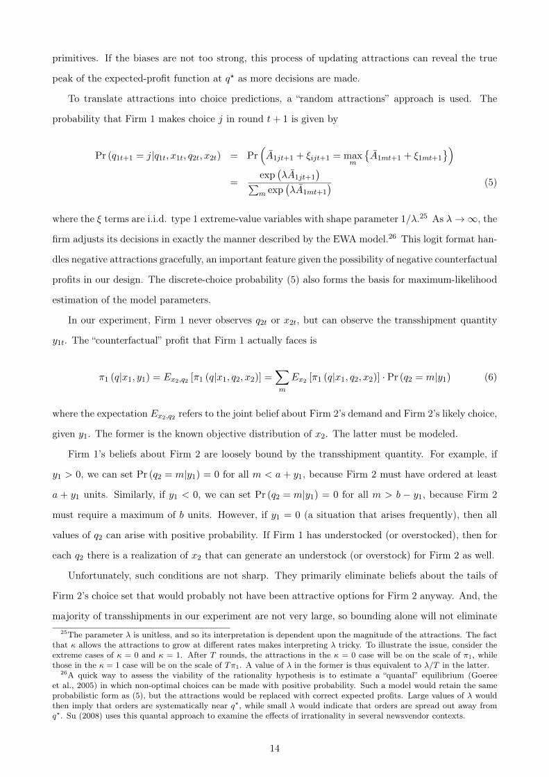
To translate attractions into choice predictions, a “random attractions” approach is used. The

probability that Firm 1 makes choice j in round t+ 1 is given by

Pr (q1t+1 = j|q1t, x1t, q2t, x2t) = Pr(A1jt+1 + ξijt+1 = max

m

{A1mt+1 + ξ1mt+1

})=

exp(λA1jt+1

)∑m exp

(λA1mt+1

) (5)

where the ξ terms are i.i.d. type 1 extreme-value variables with shape parameter 1/λ.25 As λ→∞, the

firm adjusts its decisions in exactly the manner described by the EWA model.26 This logit format han-

dles negative attractions gracefully, an important feature given the possibility of negative counterfactual

profits in our design. The discrete-choice probability (5) also forms the basis for maximum-likelihood

estimation of the model parameters.

In our experiment, Firm 1 never observes q2t or x2t, but can observe the transshipment quantity

y1t. The “counterfactual” profit that Firm 1 actually faces is

π1 (q|x1, y1) = Ex2,q2 [π1 (q|x1, q2, x2)] =∑m

Ex2 [π1 (q|x1, q2, x2)] · Pr (q2 = m|y1) (6)

where the expectation Ex2,q2 refers to the joint belief about Firm 2’s demand and Firm 2’s likely choice,

given y1. The former is the known objective distribution of x2. The latter must be modeled.

Firm 1’s beliefs about Firm 2 are loosely bound by the transshipment quantity. For example, if

y1 > 0, we can set Pr (q2 = m|y1) = 0 for all m < a + y1, because Firm 2 must have ordered at least

a + y1 units. Similarly, if y1 < 0, we can set Pr (q2 = m|y1) = 0 for all m > b − y1, because Firm 2

must require a maximum of b units. However, if y1 = 0 (a situation that arises frequently), then all

values of q2 can arise with positive probability. If Firm 1 has understocked (or overstocked), then for

each q2 there is a realization of x2 that can generate an understock (or overstock) for Firm 2 as well.

Unfortunately, such conditions are not sharp. They primarily eliminate beliefs about the tails of

Firm 2’s choice set that would probably not have been attractive options for Firm 2 anyway. And, the

majority of transshipments in our experiment are not very large, so bounding alone will not eliminate25The parameter λ is unitless, and so its interpretation is dependent upon the magnitude of the attractions. The fact

that κ allows the attractions to grow at different rates makes interpreting λ tricky. To illustrate the issue, consider theextreme cases of κ = 0 and κ = 1. After T rounds, the attractions in the κ = 0 case will be on the scale of π1, whilethose in the κ = 1 case will be on the scale of Tπ1. A value of λ in the former is thus equivalent to λ/T in the latter.

26A quick way to assess the viability of the rationality hypothesis is to estimate a “quantal” equilibrium (Goereeet al., 2005) in which non-optimal choices can be made with positive probability. Such a model would retain the sameprobabilistic form as (5), but the attractions would be replaced with correct expected profits. Large values of λ wouldthen imply that orders are systematically near q?, while small λ would indicate that orders are spread out away fromq?. Su (2008) uses this quantal approach to examine the effects of irrationality in several newsvendor contexts.

14

many possibilities.

We instead use EWA mechanics to formulate an adaptively-changing belief for Firm 1 about Firm

2. Suppose that Firm 1 enters round t with a set of attractions {B1mt}Mm=0 reflecting its beliefs about

Firm 2’s ordering strategy.27 The update to the estimated attractiveness of order quantity j to Firm

2 is

B1jt+1 =φN1tB1jt + Ex2t [π2 (j|x2t, q1t, x1t)]

N1t+1(7)

which involves only quantities that Firm 1 knows (i.e., q1t, x1t, the objective distribution of x2t, and the

counterfactual profit function π2). The behavioral primitives that affect the formation of A attractions

also affect the B attractions, except for the reinforcement bias δ. (Recall that conditioning on q1t

automatically implies δ = 1, so there is no possible reinforcement bias in beliefs.)

In a manner similar to (5), Firm 1 can formulate belief probabilities about Firm 2:

Pr (q2t+1 = j|q1t, x1t) =exp

(λB1jt+1

)∑

m exp(λB1mt+1

) (8)

Here, λ describes the extent to which Firm 1 uses the available information about Firm 2 in its update.

Because λ → 0 implies that Firm 1 ignores the available information about Firm 2, we call this bias

inattention.28 Because it seems unlikely that Firm 1 will be more sensitive to the estimated attractions

of Firm 2 than to its own attractions, we expect λ ≤ λ.

The counterfactual must also incorporate the bounding information contained in the transshipment

quantity y1t. If a transshipment occurs, these criteria automatically remove certain orders from Firm

1’s belief for period t. To accommodate this restriction, let Q (y1) denote the set of Firm 2’s order

quantities that are automatically excluded when the transshipment y1 occurs, and let Pr(Q (y1)

)denote the total probability mass (as defined by (8)) corresponding to this set. The beliefs used in the

counterfactual analysis of round t are of the form

Pr (q2t+1 = j|y1t+1) =

Pr(q2t+1=j|q1t,x1t)

1−Pr(Q(y1t+1))if j ∈ Q (y1t+1)

0 else(9)

which is the truncated distribution corresponding to (8).27To be clear, the B attractions reflect Firm 1’s adaptive best guess about Firm 2’s A attractions. Firm 1 does not

have sufficient information to compute Firm 2’s actual A attractions.28Because Firm 1 formulates these beliefs conditional on its own outcome, the B attractions can be viewed as a kind

of ex post introspective best response to its own decision. Under this reading, the parameter λ describes how well Firm1 performs this best-response task. In a similar vein, Camerer et al. (2002) describe an EWA agent that recognizesthat its partner may also be operating according to EWA mechanics. Such an agent can formulate a best response thatincorporates the probability that the partner is updating in a similar fashion. Importantly, their agent can observe thecomplete outcomes from prior interactions, while ours cannot.

15

With these beliefs, we can modify the A choice attractions in (3) to address Firm 1’s uncertainty

about x2t and q2t:

A1jt+1 =φN1tA1jt + [δ + 1 (j = q1t) (1− δ)]

∑mEx2 [π1 (j|x1t, q2t, x2t)] · Pr (q2t = m|y1t)

N1t+1(10)

Note that the counterfactual profit has been replaced with the expected counterfactual profit (6). The

probability over q2t has been constructed using the belief update described in (7)-(9).29 The choice

probabilities (5) can be reformulated by replacing the A attractions with the A attractions:

Pr (q1t+1 = j|q1t, x1t, y1t) =exp (λA1jt+1)∑m exp (λA1mt+1)

(11)

To initialize the model, we set A1j0 = B1j0 = 0 for all j = 0, . . . ,M = 200 attractions, and also set

N10 = 0. This implies that Firm 1 makes each choice with equal probability in round 1, and believes

that Firm 2 is also equally likely to make each choice. This strategy profile results in an initial median

order quantity that is located at the middle of the choice set Q, though the variability is quite high.

With this setup, the behavioral parameters affect aggregate decisions in predictable ways.30 On

average, the most recent demand realization comes from the center of the demand distribution, and

so a large recency bias will cause average orders to be biased towards central quantities. The effect of

reinforcement bias partially depends on τ . Profits can be negative if a firm makes too large an order

when τ is low (a sizable transshipment may occur, and the sending firm will incur a loss of $0.20 on each

unit transshipped), and a strong reinforcement bias will immediately lead to smaller orders to prevent

these losses. Negative profits are much less likely for similar orders when τ is high, and reinforcement

will have a less drastic effect. However, the overall effect of reinforcement is also a pull towards center,

because the average demand realization from the center involves a positive profit. Inattention causes

orders to be too high when τ is high and too low when τ is low, because ignoring the partner causes

the firm to forego profitable transshipment transactions. Finally, the logit error will tend to spread

decisions around the center of the choice set as EWA mechanics become a less-accurate description of

decision making.

In addition to these aggregate effects, EWA-style models have the benefit of capturing path-

dependence at the individual level. For example, in a no-transshipment experiment, Bostian et al.

(2008) reported that one subject ordered the maximum quantity every round. Because this strategy29When computing the ex post counterfactual profit (6), we apply the belief probabilities for round t, not those for

t+ 1. Because the belief aspect is both introspective and evolutionary, the t+ 1 beliefs can be best interpreted as Firm1’s estimate of Firm 2’s order next period. In the ex post exercise, however, we wish to use beliefs that were in place forthe current decision, which are those corresponding to Bjmt.

30We provide some numerical comparative-static simulations in Figure A.3 of the online appendix to confirm thesetendencies.

16

turned out to be somewhat profitable ex post (although certainly not profit-maximizing), a parametriza-

tion with sufficient recency and reinforcement bias replicated this pattern after just a few rounds. This

extreme case illustrates that EWA’s predictive power is not limited to large-sample effects. Outlier

data far from equilibrium can also be accommodated.

Before taking this modified EWA model to the data, we must incorporate the mirror-image treat-

ment change. Because the two treatments within a session generate incentives that are symmetric

about τ = $0.20 and q = 100, the outcome history from the first treatment is potentially very useful

for forming decisions in the second treatment. To apply the information accumulated during the first

treatment, all that is needed is to reverse the order of the attractions upon starting the second. Hence,

if a treatment change occurs after round t, we initialize new attractions A′1jt+1 = ψA1(M−j)t+1 and

B′1jt+1 = ψB1(M−j)t+1, and also set N ′1t+1 = ψN1t+1. The parameter ψ captures how much of the

information from the first treatment is carried over to the second. The case ψ = 0 implies that subjects

mentally start afresh each treatment, while ψ = 1 implies that the beliefs upon starting the second

treatment are an exact mirror image of those present at the end of the first treatment. An estimate

between 0 and 1 would indicate a partial initial adjustment consistent with a sequence effect.

The maximum-likelihood estimates for the individual cohorts and pooled dataset are provided in

Table 5. The sequence parameter ψ is about 0.7, indicating that subjects applied a substantial amount

of the learning accumulated in the first treatment to formulate their initial decisions in the second, but

did not perfectly invert their choice heuristics. The likelihood-ratio tests of the point estimates in one

model to those in another reveal a striking pattern: it is not possible to statistically reject the pooled

estimates as being operative in either cohort, but it is possible to reject one cohort’s estimates as being

operative in another’s.31 It appears that the pooled estimates provide a “happy medium” between the

individual cohort estimates. However, upon comparing the individual estimates, it is clear that the

statistical differences between the cohorts do not translate into economic significance.

The recency parameter φ is between 0.9 and 0.91 in all three cases, a value that has been previously

found in non-transshipment settings (see Bostian et al., 2008). While this value may not appear to be

substantially different from the rational value of 1, it is important to recall that its effect is a geometric

depreciation of the learning stock. As a result, a subject gives the most recent “lesson learned” a 0.9

weight in the next round, 0.95 = 0.59 weight five rounds hence, 0.910 = 0.35 weight ten rounds hence,

etc. This is, in fact, a very quick pace of forgetting.31To be clear, we apply the null hypothesis in both directions, allowing one set of estimates to serve as the null

values, and then the other set. This method addresses the fact that the null hypothesis is itself being generated froman estimate. This is a particularly important consideration when comparing pooled results to cohort results, becausethe pooled variance will be smaller by the simple virtue of its doubled sample size. The pooled estimates thus have apredetermined advantage as the alternative hypothesis.

17

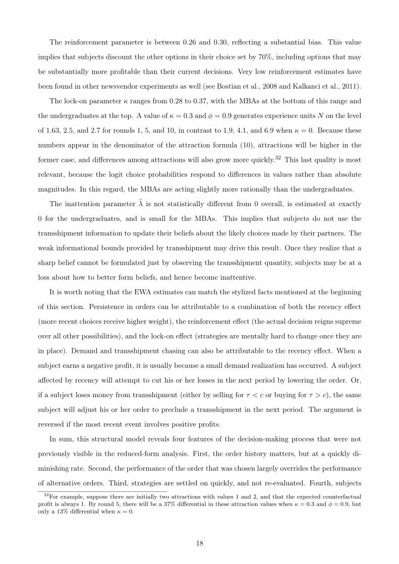
The reinforcement parameter is between 0.26 and 0.30, reflecting a substantial bias. This value

implies that subjects discount the other options in their choice set by 70%, including options that may

be substantially more profitable than their current decisions. Very low reinforcement estimates have

been found in other newsvendor experiments as well (see Bostian et al., 2008 and Kalkanci et al., 2011).

The lock-on parameter κ ranges from 0.28 to 0.37, with the MBAs at the bottom of this range and

the undergraduates at the top. A value of κ = 0.3 and φ = 0.9 generates experience units N on the level

of 1.63, 2.5, and 2.7 for rounds 1, 5, and 10, in contrast to 1.9, 4.1, and 6.9 when κ = 0. Because these

numbers appear in the denominator of the attraction formula (10), attractions will be higher in the

former case, and differences among attractions will also grow more quickly.32 This last quality is most

relevant, because the logit choice probabilities respond to differences in values rather than absolute

magnitudes. In this regard, the MBAs are acting slightly more rationally than the undergraduates.

The inattention parameter λ is not statistically different from 0 overall, is estimated at exactly

0 for the undergraduates, and is small for the MBAs. This implies that subjects do not use the

transshipment information to update their beliefs about the likely choices made by their partners. The

weak informational bounds provided by transshipment may drive this result. Once they realize that a

sharp belief cannot be formulated just by observing the transshipment quantity, subjects may be at a

loss about how to better form beliefs, and hence become inattentive.

It is worth noting that the EWA estimates can match the stylized facts mentioned at the beginning

of this section. Persistence in orders can be attributable to a combination of both the recency effect

(more recent choices receive higher weight), the reinforcement effect (the actual decision reigns supreme

over all other possibilities), and the lock-on effect (strategies are mentally hard to change once they are

in place). Demand and transshipment chasing can also be attributable to the recency effect. When a

subject earns a negative profit, it is usually because a small demand realization has occurred. A subject

affected by recency will attempt to cut his or her losses in the next period by lowering the order. Or,

if a subject loses money from transshipment (either by selling for τ < c or buying for τ > c), the same

subject will adjust his or her order to preclude a transshipment in the next period. The argument is

reversed if the most recent event involves positive profits.

In sum, this structural model reveals four features of the decision-making process that were not

previously visible in the reduced-form analysis. First, the order history matters, but at a quickly di-

minishing rate. Second, the performance of the order that was chosen largely overrides the performance

of alternative orders. Third, strategies are settled on quickly, and not re-evaluated. Fourth, subjects32For example, suppose there are initially two attractions with values 1 and 2, and that the expected counterfactual

profit is always 1. By round 5, there will be a 37% differential in these attraction values when κ = 0.3 and φ = 0.9, butonly a 13% differential when κ = 0.

18

largely discard the informational content provided by the transshipment quantity. These behavioral

features will be at the core of the counterfactual analysis of transshipment efficacy.

5.2 Forward Thinking via Cognitive Hierarchy

Although the EWA mechanics can eventually uncover q?, the model assumes that the firm does not

undertake any profit-maximization analysis on its own. Instead, it must engage in a largely trial-and-

error process to discover its own expected-profit function. Because this may not be a descriptive model

of managerial skill, we explore an alternative forward-thinking model of decision making. This model

does not require any choice or outcome history as input, and so it is unlikely to generate predictions

that replicate the stylized facts noted earlier. However, it will play a role when we examine the behavior

of individuals, so we outline it here.

In the Poisson CH model by Camerer et al. (2004), choices are determined through an iterative

mental process. The step at which the firm stops iterating reflects its “level of rationality.” In each

step of the process, the firm believes it is the more rational agent in the game. Denote the rationality

level of Firms 1 and 2 by r1 and r2, and consider the process from the perspective of Firm 1. Let the

probability of each rationality level be P (r; θ), a Poisson distribution with mean/variance parameter

θ. The levels in the cognitive hierarchy are described by recursively-defined probability distributions.

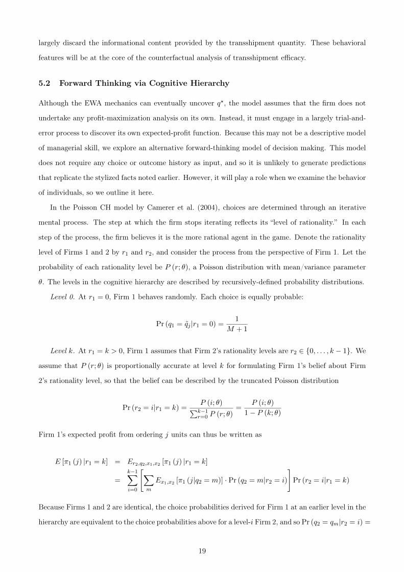
Level 0. At r1 = 0, Firm 1 behaves randomly. Each choice is equally probable:

Pr (q1 = qj |r1 = 0) =1

M + 1

Level k. At r1 = k > 0, Firm 1 assumes that Firm 2’s rationality levels are r2 ∈ {0, . . . , k − 1}. We

assume that P (r; θ) is proportionally accurate at level k for formulating Firm 1’s belief about Firm

2’s rationality level, so that the belief can be described by the truncated Poisson distribution

Pr (r2 = i|r1 = k) =P (i; θ)∑k−1r=0 P (r; θ)

=P (i; θ)

1− P (k; θ)

Firm 1’s expected profit from ordering j units can thus be written as

E [π1 (j) |r1 = k] = Er2,q2,x1,x2 [π1 (j) |r1 = k]

=k−1∑i=0

[∑m

Ex1,x2 [π1 (j|q2 = m)] · Pr (q2 = m|r2 = i)

]Pr (r2 = i|r1 = k)

Because Firms 1 and 2 are identical, the choice probabilities derived for Firm 1 at an earlier level in the

hierarchy are equivalent to the choice probabilities above for a level-i Firm 2, and so Pr (q2 = qm|r2 = i) =

19

Pr (q1 = qm|r1 = i). These expected profits translate into choice probabilities for level k in the hierar-

chy via logits:33

Pr (q1 = j|r1 = k) =exp (σE [π1 (j) |r1 = k])∑m exp (σE [π1 (j) |r1 = k])

Finally, the probability that a level-k Firm 1 observes the order j by Firm 2 is

Pr (q2 = j|r1 = k) = Er2 [Pr (q2 = j|r2 < k)] =k−1∑i=0

Pr (q2 = j|r2 = i) Pr (r2 = i|r1 = k) (12)

Because our newsvendor model is discretized, the optimal order quantity can be discovered in a

finite number of steps of perfect mental best response: about 8 steps when starting from q = 0, and

about 6 steps when starting from q = 100. As a result, we set an upper bound of K = 8 levels of

rationality for this model, which should capture the most rational, profit-maximizing behavior.34

The values of θ and σ have predictable effects on choices.35 First, the logit error will spread decisions

around the center of the demand distribution if CH fits poorly. Second, the choice distributions will be

quite different at each level of the hierarchy when moving out of the low rationality levels (e.g., k = 0 to

k = 1, and k = 1 to k = 2), but very similar when moving to higher levels (e.g., k = 2 to k = 3). Most

of the improvement in profitability arises from replacing purely random choices with better informed

choices; further improvements eventually become minor refinements with smaller profit impacts. And,

if θ is small, not many of these higher-level refinements will be made.

In addition, the choice distributions will never be centered exactly at q?. To see the intuition

for this result, consider the τ = $0.40 treatment. The average level-0 choice is located at the center

of the demand distribution. The level-1 strategy takes advantage of this consistent under-ordering

by over-ordering, because the likelihood of making a profitable transshipment has increased. An

immediate level-2 response to the level-1 strategy involves under-ordering to exactly counter this over-

ordering. However, the level-2 firm assumes that its partner could be either level-0 or level-1, and so

it best-responds to a weighted mixture of level-0 and level-1 strategies. This makes the amount of

under-ordering in level 2 somewhat less pronounced. Best responses in levels 3 and higher involve a

similar weighted mixture of all lower-level strategies. Because all lower-level strategies are biased away

from the optimum, the strategy for any level k must also involve some (diminishing) bias.

Table 6 provides maximum-likelihood estimates of θ and σ for each cohort and the pooled dataset.33The CH model can also be formulated without stochastic choice for k > 0, in which case a level-k firm perfectly best-

responds at each level of the hierarchy, making only the choice with the highest expected profit. All other possibilitiesare relegated to level-0 status. Eliminating stochastic choice here would imply that small (e.g., 1-unit) order deviationsfrom level-k predictions would be characterized as level 0. In our setting with 201 possible order quantities, these smalldeviations should probably not be taken as strong evidence against level-k thinking.

34Imposing K = 8 appears to be empirically innocuous. Our estimates imply that at most 5% of the probability massof P lies above K = 8, so this boundary probably does not bias the choice probabilities very much.

35We provide some numerical comparative-static simulations in the online appendix to confirm these tendencies.

20

We find that it is always possible to reject the hypothesis that any cohort’s point estimates are identical

to any others’. The estimated values of θ are around 2.86 and 2.91, which does not reflect very many

steps of forward thinking. Undergraduate subjects tend to exhibit slightly more noise than do the

MBA subjects, but otherwise both cohorts again appear to be quite similar with respect to σ.

These rather lackluster estimates confirm our earlier intuition regarding the applicability of the

CH model. For a more rigorous examination, Table 7 provides values of the Bayesian Information

Criterion (BIC) for the two models. Recall that BIC = −2ll + (#parameters) ln (#observations),

where ll denotes the total log-likelihood of the model. The selection rule chooses the model with the

smallest BIC value, because it has the highest likelihood of explaining the data after accounting for

model parsimony. In all three cases, the criterion shows EWA to be best explanation of the data by far.

Thus, our subjects do not appear to be forward-thinking at all, instead adopting the empirical-learning

approach.

In addition, it does not seem that the forward-thinking framework can be rescued by enhancing it

with adaptive features. In the online appendix, we present results of a “sophisticated” CH firm that

can perform both adaptive and level-k reasoning, and realizes that its partner may be of either type.

If this sophisticated firm has a sufficiently strong belief that its partner is adaptive, it will adjust its

orders to account for its partner’s adaptivity, and so its decisions will exhibit some dependence on

history. In taking this model to the data, we find that the parameter estimates are very close to those

of a pure-CH firm, and that the BIC statistics improve only slightly from their original CH values.

Thus, adaptivity seems to be the best explanation for our data.

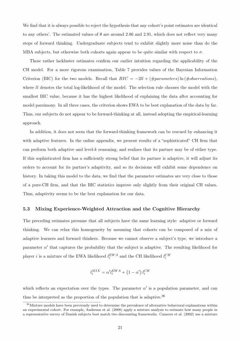
5.3 Mixing Experience-Weighted Attraction and the Cognitive Hierarchy

The preceding estimates presume that all subjects have the same learning style: adaptive or forward

thinking. We can relax this homogeneity by assuming that cohorts can be composed of a mix of

adaptive learners and forward thinkers. Because we cannot observe a subject’s type, we introduce a

parameter α′ that captures the probability that the subject is adaptive. The resulting likelihood for

player i is a mixture of the EWA likelihood lEWAi and the CH likelihood lCHi

lMIXi = α′lEWA

i +(1− α′

)lCHi

which reflects an expectation over the types. The parameter α′ is a population parameter, and can

thus be interpreted as the proportion of the population that is adaptive.36

36Mixture models have been previously used to determine the prevalence of alternative behavioral explanations withinan experimental cohort. For example, Andersen et al. (2008) apply a mixture analysis to estimate how many people ina representative survey of Danish subjects best match two discounting frameworks. Camerer et al. (2002) use a mixture

21

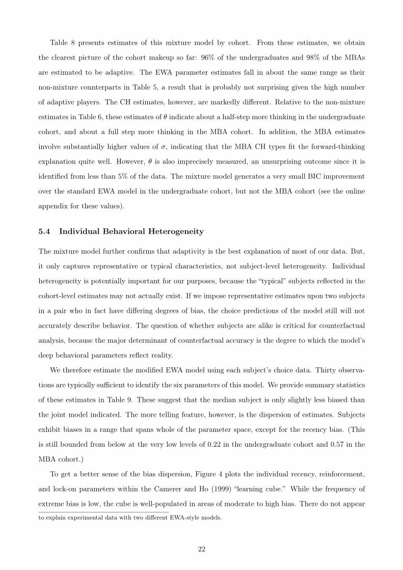
Table 8 presents estimates of this mixture model by cohort. From these estimates, we obtain

the clearest picture of the cohort makeup so far: 96% of the undergraduates and 98% of the MBAs

are estimated to be adaptive. The EWA parameter estimates fall in about the same range as their

non-mixture counterparts in Table 5, a result that is probably not surprising given the high number

of adaptive players. The CH estimates, however, are markedly different. Relative to the non-mixture

estimates in Table 6, these estimates of θ indicate about a half-step more thinking in the undergraduate

cohort, and about a full step more thinking in the MBA cohort. In addition, the MBA estimates

involve substantially higher values of σ, indicating that the MBA CH types fit the forward-thinking

explanation quite well. However, θ is also imprecisely measured, an unsurprising outcome since it is

identified from less than 5% of the data. The mixture model generates a very small BIC improvement

over the standard EWA model in the undergraduate cohort, but not the MBA cohort (see the online

appendix for these values).

5.4 Individual Behavioral Heterogeneity

The mixture model further confirms that adaptivity is the best explanation of most of our data. But,

it only captures representative or typical characteristics, not subject-level heterogeneity. Individual

heterogeneity is potentially important for our purposes, because the “typical” subjects reflected in the

cohort-level estimates may not actually exist. If we impose representative estimates upon two subjects

in a pair who in fact have differing degrees of bias, the choice predictions of the model still will not

accurately describe behavior. The question of whether subjects are alike is critical for counterfactual

analysis, because the major determinant of counterfactual accuracy is the degree to which the model’s

deep behavioral parameters reflect reality.

We therefore estimate the modified EWA model using each subject’s choice data. Thirty observa-

tions are typically sufficient to identify the six parameters of this model. We provide summary statistics

of these estimates in Table 9. These suggest that the median subject is only slightly less biased than

the joint model indicated. The more telling feature, however, is the dispersion of estimates. Subjects

exhibit biases in a range that spans whole of the parameter space, except for the recency bias. (This

is still bounded from below at the very low levels of 0.22 in the undergraduate cohort and 0.57 in the

MBA cohort.)

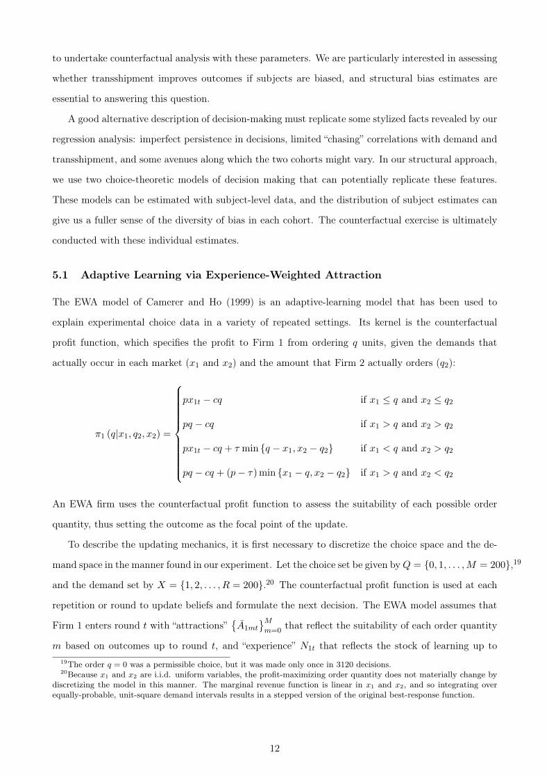
To get a better sense of the bias dispersion, Figure 4 plots the individual recency, reinforcement,

and lock-on parameters within the Camerer and Ho (1999) “learning cube.” While the frequency of

extreme bias is low, the cube is well-populated in areas of moderate to high bias. There do not appear

to explain experimental data with two different EWA-style models.

22

to be any meaningful clusters of bias, nor material differences in the location of undergraduates and

MBAs within the cube. It is quite a heterogenous set of subjects.

We also obtain individual estimates of the CH parameters, and find that θ similarly runs in a wide

range (see the online appendix for these values). While the α′ estimates indicate that forward thinking

is probably not a good description of our cohort as a whole, the individual CH estimates allow us to

perform subject-level discrimination with the BIC. In that analysis, we find strong support for the

EWA model in all but six subjects, three undergraduates and three MBAs. This implies that 94% of

each cohort is adaptive, a percentage quite close to the estimated α′. Two forward-thinking subjects

were actually paired together, and the others were paired with adaptive partners.37

6 No-Transshipment Counterfactual Analysis

Our structural estimates indicate that our subjects can be described as heterogeneously-biased, adap-

tive decision makers. One natural question that arises is whether transshipment can have any useful

application in the presence of behavior that significantly departs from optimal predictions. Fortunately,

our structural model allows us to construct a relevant counterfactual: how would profits have changed

if transshipment had not been allowed?38

To conduct this counterfactual, we compare individual profit predictions of an EWA model that

allows transshipment to one that does not. In generating these predictions (expected values formulated

from choice probabilities), we use the same demand realizations that subjects actually faced, along with

their individually-estimated EWA parameters.39 Summary statistics for this exercise are reported in

Table 10. Recall from Table 2 that transshipment should theoretically generate profits about 28%

higher in the τ = $0.00 and $0.40 treatments, and about 32% higher in the τ = $0.10 and $0.30

treatments. Because subjects are significantly biased from the optimum, the actual effect is much

stronger: median counterfactual profit improvements are about 40% for undergraduates, and 37% for

MBAs. This benefit varies quite a bit, as illustrated by the rather large standard deviations, but all

subjects have substantive counterfactual improvements.

Interestingly, transshipment has a much stronger benefit in the presence of biases than in their

absence. For the median subject, the counterfactual percentage increase in profit arising from the37We also hoped to compare the profits of the EWA and CH players, but comparing 5% of subjects to the other 95%

is a statistically weak analysis.38It is difficult to address this question experimentally by having the same subjects participate in both transshipment

and no-transshipment designs. Both have substantial overlap in their game structures, and it would thus be difficult todisentangle the transshipment effect from those arising from earlier exposure to a similar set of incentives.

39We do not compare the actual profits with transshipment to the predicted profits without transshipment. Becauseno model can perfectly fit the data, actual profits contain some additional statistical noise. This noise is impossible toreplicate in the counterfactual, because we do not know how it would have changed under no-transshipment incentives.

23

implementation of transshipment exceeds the theoretical improvement by a quarter to almost a half.

The mitigation of behavioral bias is an unintended benefit of the transshipment arrangement. Although

transshipment theory does not focus very much on what occurs outside of equilibrium, there may be

additional benefits to be explored in this vein.

7 Conclusion

Our analysis suggests that transshipment mitigates behavioral bias. A question that still remains,

however, is whether decision-makers in real supply chains are susceptible to biases similar to those found

in our experimental subjects. Our two-cohort design – one with MBAs and one with undergraduates

– gives us the opportunity to assess whether bias is merely a transient effect that can be mitigated

through professional experience. The evidence indicates that professional experience does not matter

at all. The MBAs look very much like the undergraduates in their bias profile: both cohorts exhibit

moderate recency bias, high reinforcement bias, fast lock-on, and inattention to implicit strategic

information coming from their partners. Even with the opportunity to learn about incentives through

repeated interactions, these biases would cause decisions to move away from the optimum, lowering

profits. Transshipment recaptures some of this lost profit.

Of course, managers are extensively trained in firm- and industry-specific practices, and it is possible

that mastery of such specialized knowledge is a more important factor in determining whether a supply

chain is well-run. Experienced supply-chain managers may also have different bias profiles than our

MBA subjects, who came from diverse professional backgrounds. However, Bolton et al. (forthcoming)

report that undergraduates, graduates, and professionals all seem to fall prey to the pull-to-center

effect in the single-retailer setting, further bolstering the idea that some biases are fundamental. Our

results suggest that rather than investing more extensively in training or experience, firms may generate

higher returns by investing in behaviorally-robust supply-chain strategies such as transshipment, or by

deploying them on a wider scale.

References

Steffen Andersen, Glenn W. Harrison, Morten I. Lau, and E. Elisabet Rutström. Eliciting risk andtime preferences. Econometrica, 76(3):583–618, May 2008.

J. Neil Bearden, Ryan O. Murphy, and Amnon Rapoport. Decision biases in revenue management:Some behavioral evidence. Manufacturing and Service Operations Management, 10(4):625–636, Fall2008.

Elliot Bendoly, Karen Donohue, and Kenneth L. Schultz. Behavior in operations management: As-

24

sessing recent findings and revisiting old assumptions. Journal of Operations Management, 24(6):737–752, December 2006.

Gary E. Bolton and Elena Katok. Learning by doing in the newsvendor problem: A laboratory inves-tigation of the role of experience and feedback. Manufacturing and Service Operations Management,10(3):519–538, Summer 2008.

Gary E. Bolton, Axel Ockenfels, and Ulrich Thonemann. Managers and students as newsvendors.Management Science, forthcoming.

AJ A. Bostian, Charles A. Holt, and Angela M. Smith. Newsvendor "pull-to-center" effect: Adaptivelearning in a laboratory experiment. Manufacturing and Services Operations Management, 10(4):590–608, Fall 2008.

Colin F. Camerer and Teck-Hua Ho. Experience-weighted attraction learning in normal-form games.Econometrica, 67(4):827–874, July 1999.

Colin F. Camerer, Teck-Hua Ho, and Juin-Kuan Chong. Sophisticated experience-weighted attractionlearning and strategic teaching in repeated games. Journal of Economic Theory, 104(1):1–52, May2002.

Colin F. Camerer, Teck-Hua Ho, and Juin-Kuan Chong. A cognitive hierarchy model of games. Quar-terly Journal of Economics, 119(3):861–898, August 2004.

Rachel Croson and Karen Donohue. Experimental economics and supply-chain management. Interfaces,32(5):74–82, September 2002.

Rachel Croson and Karen Donohue. Behavioral causes of the bullwhip effect and the observed valueof inventory information. Management Science, 53(3):323–336, March 2006.

Rachel Croson, Karen Donohue, Elena Katok, and John Sterman. Order stability in supply chains:Coordination risk and the role of coordination stock. Working paper, University of Pennsylvania,July 2005.

Francis de Véricourt, J. Neil Bearden, and Allan Filipowicz. Sex, risk, and the newsvendor. Workingpaper, INSEAD Singapore, June 2011.

Lingxiu Dong and Nils Rudi. Who benefits from transshipment? Exogenous vs. endogenous wholesaleprices. Management Science, 50(5):645–657, May 2004.

Guillaume R. Fréchette. Laboratory experiments: Professionals versus students. In Guillaume R.Fréchette and Andrew Schotter, editors, The Methods of Modern Experimental Economics. OxfordUniversity Press, forthcoming.

Noah Gans and Rachel Croson. Introduction to the special issue on behavioral operations. Manufac-turing and Services Operations Management, 10(4):573–565, Fall 2008.

Francesca Gino and Gary Pisano. Toward a theory of behavioral operations. Manufacturing andService Operations Management, 10(4):676–691, Fall 2008.

Jacob K. Goeree, Charles A. Holt, and Thomas R. Palfrey. Regular quantal response equilibrium.Experimental Economics, 8(4):347–367, December 2005.

Teck-Hua Ho, Noah Lim, and Tony Haitao Cui. Reference dependence in multilocation newsvendormodels: A structural analysis. Management Science, 56(11), November 2010.

Xinxin Hu, Izak Duenyas, and Roman Kapuscinski. Existence of coordinating transshipment prices ina two-location inventory model. Management Science, 53(8):1289–1302, August 2007.

25

Basak Kalkanci, Kay-Yut Chen, and Feryal Erhun. Contract complexity and performance under asym-metric demand information: An experimental evaluation. Management Science, 57(4):689–704, April2011.

Nicholas H. Lurie and Jayashankar M. Swaminathan. Is timely information always better? The effectof feedback frequency on decision making. Organizational Behavior and Human Decision Processes,108(2):315–329, March 2009.

Nils Rudi and David Drake. Observation bias: The impact of demand censoring on newsvendor leveland adjustment behavior. Management Science, forthcoming.

Nils Rudi, Sandeep Kapur, and David F. Pyke. A two-location inventory model with transshipmentand local decision making. Management Science, 47(12):1668–1680, December 2001.

Maurice E. Schweitzer and Gérard P. Cachon. Decision bias in the newsvendor experiment with aknown demand distribution: Experimental evidence. Management Science, 46(3):404–420, March2000.

Xuanming Su. Bounded rationality in newsvendor models. Manufacturing and Service OperationsManagement, 10(4):566–589, Fall 2008.

Jun Zhang. Transshipment and its impact on supply chain members’ performance. ManagementScience, 51(10):1534–1539, October 2005.

26

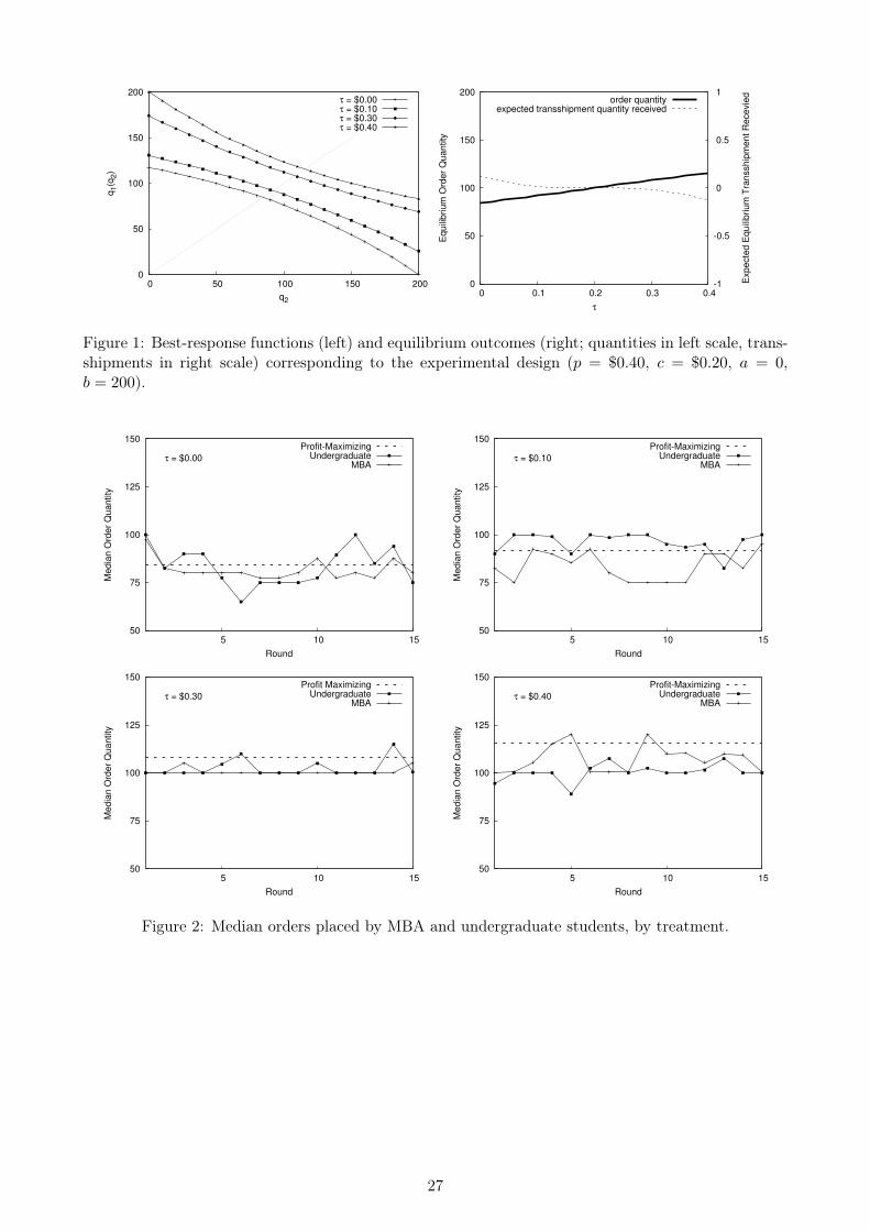
0

50

100

150

200

0 50 100 150 200

q1(q

2)

q2

τ = $0.00τ = $0.10τ = $0.30τ = $0.40

0

50

100

150

200

0 0.1 0.2 0.3 0.4-1

-0.5

0

0.5

1

Eq

uili

briu

m O

rde

r Q

ua

ntity

Exp

ecte

d E

qu

ilib

riu

m T

ran

ssh

ipm

en

t R

ece

vie

d

τ

order quantityexpected transshipment quantity received

Figure 1: Best-response functions (left) and equilibrium outcomes (right; quantities in left scale, trans-shipments in right scale) corresponding to the experimental design (p = $0.40, c = $0.20, a = 0,b = 200).

50

75

100

125

150

5 10 15

Me

dia

n O

rde

r Q

ua

ntity

Round

τ = $0.00

Profit-MaximizingUndergraduate

MBA

50

75

100

125

150

5 10 15

Me

dia

n O

rde

r Q

ua

ntity

Round

τ = $0.10

Profit-MaximizingUndergraduate

MBA

50

75

100

125

150

5 10 15

Me

dia

n O

rde

r Q

ua

ntity

Round

τ = $0.30

Profit MaximizingUndergraduate

MBA

50

75

100

125

150

5 10 15

Me

dia

n O

rde

r Q

ua

ntity

Round

τ = $0.40

Profit-MaximizingUndergraduate

MBA

Figure 2: Median orders placed by MBA and undergraduate students, by treatment.

27

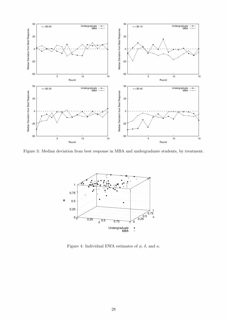
-50

-25

0

25

50

5 10 15

Me

dia

n D

evia

tio

n f

rom

Be

st

Re

sp

on

se

Round

τ = $0.00 UndergraduateMBA

-50

-25

0

25

50

5 10 15

Me

dia

n D

evia

tio

n f

rom

Be

st

Re

sp

on

se

Round

τ = $0.10 UndergraduateMBA

-50

-25

0

25

50

5 10 15

Me

dia

n D

evia

tio

n f

rom

Be

st

Re

sp

on

se

Round

τ = $0.30 UndergraduateMBA

-50

-25

0

25

50

5 10 15

Me

dia

n D

evia

tio

n f

rom

Be

st

Re

sp

on

se

Round

τ = $0.40 UndergraduateMBA

Figure 3: Median deviation from best response in MBA and undergraduate students, by treatment.

0 0.25 0.5 0.75 1 0 0.25

0.5 0.75

1

0

0.25

0.5

0.75

1

φ

UndergraduateMBA

δ

κ

φ

Figure 4: Individual EWA estimates of φ, δ, and κ.

28

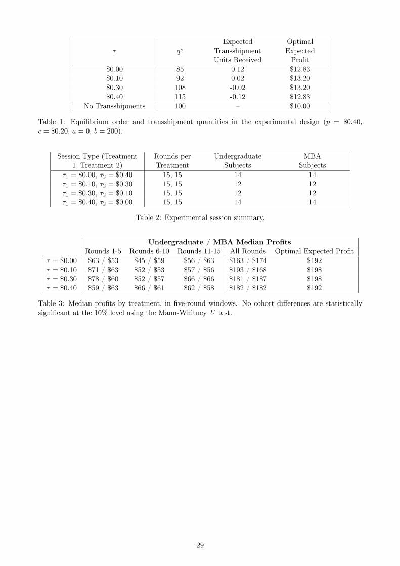
τ q?Expected

TransshipmentUnits Received

OptimalExpectedProfit

$0.00 85 0.12 $12.83$0.10 92 0.02 $13.20$0.30 108 -0.02 $13.20$0.40 115 -0.12 $12.83

No Transshipments 100 – $10.00

Table 1: Equilibrium order and transshipment quantities in the experimental design (p = $0.40,c = $0.20, a = 0, b = 200).

Session Type (Treatment1, Treatment 2)

Rounds perTreatment

UndergraduateSubjects

MBASubjects

τ1 = $0.00, τ2 = $0.40 15, 15 14 14τ1 = $0.10, τ2 = $0.30 15, 15 12 12τ1 = $0.30, τ2 = $0.10 15, 15 12 12τ1 = $0.40, τ2 = $0.00 15, 15 14 14

Table 2: Experimental session summary.

Undergraduate / MBA Median ProfitsRounds 1-5 Rounds 6-10 Rounds 11-15 All Rounds Optimal Expected Profit

τ = $0.00 $63 / $53 $45 / $59 $56 / $63 $163 / $174 $192τ = $0.10 $71 / $63 $52 / $53 $57 / $56 $193 / $168 $198τ = $0.30 $78 / $60 $52 / $57 $66 / $66 $181 / $187 $198τ = $0.40 $59 / $63 $66 / $61 $62 / $58 $182 / $182 $192

Table 3: Median profits by treatment, in five-round windows. No cohort differences are statisticallysignificant at the 10% level using the Mann-Whitney U test.

29

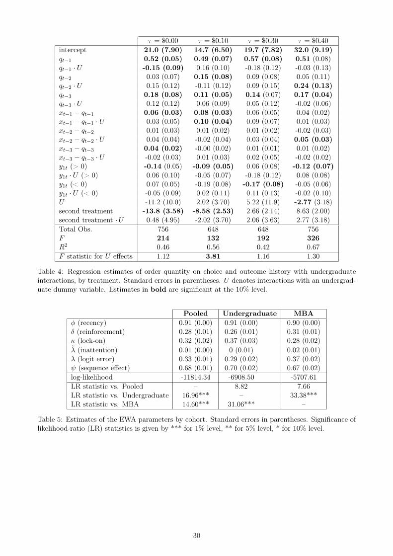
τ = $0.00 τ = $0.10 τ = $0.30 τ = $0.40

intercept 21.0 (7.90) 14.7 (6.50) 19.7 (7.82) 32.0 (9.19)qt−1 0.52 (0.05) 0.49 (0.07) 0.57 (0.08) 0.51 (0.08)qt−1 · U -0.15 (0.09) 0.16 (0.10) -0.18 (0.12) -0.03 (0.13)qt−2 0.03 (0.07) 0.15 (0.08) 0.09 (0.08) 0.05 (0.11)qt−2 · U 0.15 (0.12) -0.11 (0.12) 0.09 (0.15) 0.24 (0.13)qt−3 0.18 (0.08) 0.11 (0.05) 0.14 (0.07) 0.17 (0.04)qt−3 · U 0.12 (0.12) 0.06 (0.09) 0.05 (0.12) -0.02 (0.06)xt−1 − qt−1 0.06 (0.03) 0.08 (0.03) 0.06 (0.05) 0.04 (0.02)xt−1 − qt−1 · U 0.03 (0.05) 0.10 (0.04) 0.09 (0.07) 0.01 (0.03)xt−2 − qt−2 0.01 (0.03) 0.01 (0.02) 0.01 (0.02) -0.02 (0.03)xt−2 − qt−2 · U 0.04 (0.04) -0.02 (0.04) 0.03 (0.04) 0.05 (0.03)xt−3 − qt−3 0.04 (0.02) -0.00 (0.02) 0.01 (0.01) 0.01 (0.02)xt−3 − qt−3 · U -0.02 (0.03) 0.01 (0.03) 0.02 (0.05) -0.02 (0.02)y1t (> 0) -0.14 (0.05) -0.09 (0.05) 0.06 (0.08) -0.12 (0.07)y1t · U (> 0) 0.06 (0.10) -0.05 (0.07) -0.18 (0.12) 0.08 (0.08)y1t (< 0) 0.07 (0.05) -0.19 (0.08) -0.17 (0.08) -0.05 (0.06)y1t · U (< 0) -0.05 (0.09) 0.02 (0.11) 0.11 (0.13) -0.02 (0.10)U -11.2 (10.0) 2.02 (3.70) 5.22 (11.9) -2.77 (3.18)second treatment -13.8 (3.58) -8.58 (2.53) 2.66 (2.14) 8.63 (2.00)second treatment ·U 0.48 (4.95) -2.02 (3.70) 2.06 (3.63) 2.77 (3.18)Total Obs.FR2

7562140.46

6481320.56

6481920.42

7563260.67

F statistic for U effects 1.12 3.81 1.16 1.30

Table 4: Regression estimates of order quantity on choice and outcome history with undergraduateinteractions, by treatment. Standard errors in parentheses. U denotes interactions with an undergrad-uate dummy variable. Estimates in bold are significant at the 10% level.

Pooled Undergraduate MBAφ (recency) 0.91 (0.00) 0.91 (0.00) 0.90 (0.00)δ (reinforcement) 0.28 (0.01) 0.26 (0.01) 0.31 (0.01)κ (lock-on) 0.32 (0.02) 0.37 (0.03) 0.28 (0.02)λ (inattention) 0.01 (0.00) 0 (0.01) 0.02 (0.01)λ (logit error) 0.33 (0.01) 0.29 (0.02) 0.37 (0.02)ψ (sequence effect) 0.68 (0.01) 0.70 (0.02) 0.67 (0.02)log-likelihood -11814.34 -6908.50 -5707.61LR statistic vs. Pooled – 8.82 7.66LR statistic vs. Undergraduate 16.96*** – 33.38***LR statistic vs. MBA 14.60*** 31.06*** –

Table 5: Estimates of the EWA parameters by cohort. Standard errors in parentheses. Significance oflikelihood-ratio (LR) statistics is given by *** for 1% level, ** for 5% level, * for 10% level.

30

Pooled Undergraduate MBAθ (average rationality) 2.86 (0.10) 2.89 (0.25) 2.91 (0.09)σ (logit error) 0.57 (0.01) 0.46 (0.02) 0.70 (0.02)log-likelihood -15322.50 -7766.52 -7535.48LR statistic vs. Pooled – 19.28*** 21.76***LR statistic vs. Undergraduate 37.02*** – 77.12***LR statistic vs. MBA 45.32*** 86.32*** –

Table 6: Estimates of CH parameters by cohort. Standard errors in parentheses. Significance oflikelihood-ratio (LR) statistics given by *** for 1% level, ** for 5% level, * for 10% level.

Pooled Undergraduate MBAEWA 23676.27 12241.11 11459.33CH 30661.09 15547.74 15085.66

Table 7: BIC statistics for EWA and CH models. The smallest BIC within a cohort is bold.

Pooled Undergraduate MBAα′ (proportion EWA) 0.98 (0.01) 0.96 (0.02) 0.98 (0.03)φ (recency) 0.91 (0.00) 0.91 (0.00) 0.90 (0.00)δ (reinforcement) 0.28 (0.01) 0.28 (0.01) 0.30 (0.01)κ (lock-on) 0.32 (0.02) 0.38 (0.03) 0.28 (0.02)λ (inattention) 0.01 (0.00) 0 (0.01) 0.02 (0.01)λ (EWA logit error) 0.33 (0.01) 0.30 (0.02) 0.38 (0.02)ψ (sequence effect) 0.67 (0.01) 0.71 (0.02) 0.66 (0.02)θ (average rationality) 3.83 (1.74) 3.22 (31.8) 3.94 (27.3)σ (CH logit error) 3.88 (0.70) 0.21 (0.46) 3.35 (0.02)log-likelihood -11798.26 -6086.63 -5698.25LR statistic vs. Pooled – 18.20** 8.58LR statistic vs. Undergraduate 23.06*** – 49.82***LR statistic vs. MBA 8.58 43.24*** –

Table 8: Estimates of mixture EWA/CH model parameters by cohort. Standard errors in parentheses.Significance of likelihood-ratio (LR) statistics given by *** for 1% level, ** for 5% level, * for 10%level.

Undergraduate MBAMedian St. Dev. Min Max Median St. Dev. Min Max

φ (recency) 0.974 0.145 0.219 1 0.970 0.105 0.571 1δ (reinforcement) 0.409 0.243 0 1 0.386 0.230 0 1κ (lock-on) 0.258 0.344 0 1 0.265 0.392 0 1λ (inattention) 0.026 0.827 0 3.156 0.083 0.843 0 3.551λ (logit error) 0.396 0.386 0.020 1.775 0.441 0.553 0.098 3.866ψ (sequence effect) 0.729 0.405 0 1 0.805 0.397 0 1

Table 9: Summary statistics of individual EWA estimates within the experimental cohort.

31

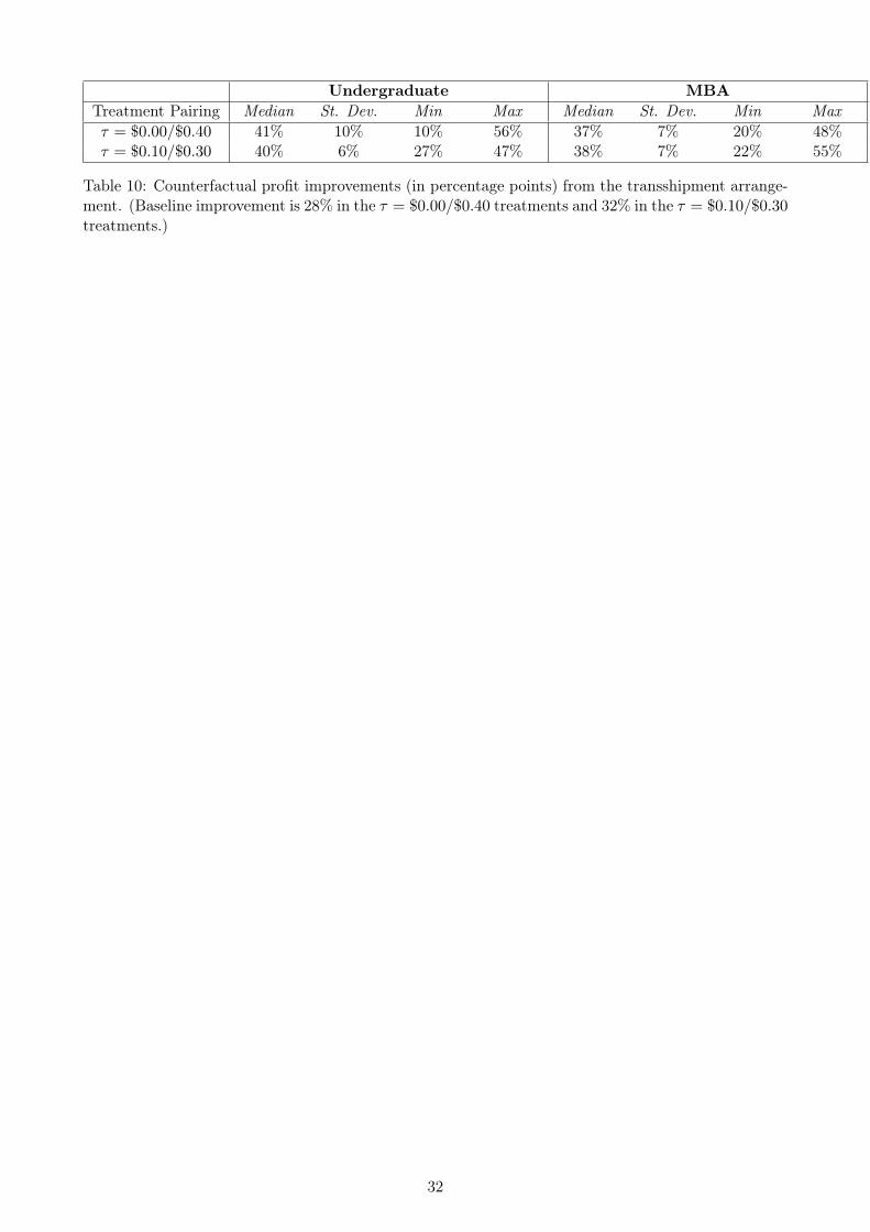
Undergraduate MBATreatment Pairing Median St. Dev. Min Max Median St. Dev. Min Maxτ = $0.00/$0.40 41% 10% 10% 56% 37% 7% 20% 48%τ = $0.10/$0.30 40% 6% 27% 47% 38% 7% 22% 55%

Table 10: Counterfactual profit improvements (in percentage points) from the transshipment arrange-ment. (Baseline improvement is 28% in the τ = $0.00/$0.40 treatments and 32% in the τ = $0.10/$0.30treatments.)

32

A Online Appendix

A.1 Orders and Best-Response Errors in Five-Round Windows

Undergraduate / MBA Median Order QuantitiesRounds 1-5 Rounds 6-10 Rounds 11-15 All Rounds q?

τ = $0.00 87 / 80 75 / 80 90 / 80 80 / 80 84τ = $0.10 100 / 85 100 / 80 100 / 83 100 / 80 92τ = $0.30 100 / 100 100 / 100 101 / 100 100 / 100 108τ = $0.40 100 / 105 100 / 110 100 / 110 100 / 110 116

Table A.1: Median order quantities by treatment, in five-round windows. Pairs in bold reflect asignificant group difference at the 10% level using the Mann-Whitney U test.

Undergraduate / MBA Median Best-Response ErrorsRounds 1-5 Rounds 6-10 Rounds 11-15 All Rounds

τ = $0.00 24 / 22 26 / 21 26 / 20 24 / 21τ = $0.10 23 / 27 24 / 26 18 / 23 22 / 25τ = $0.30 22 / 29 23 / 19 22 / 25 22 / 25τ = $0.40 34 / 20 24 / 21 26 / 21 29 / 20

Table A.2: Median absolute-value best-response errors by treatment, in five-round windows. Pairs inbold reflect a significant group difference at the 10% level using the Mann-Whitney test.

33

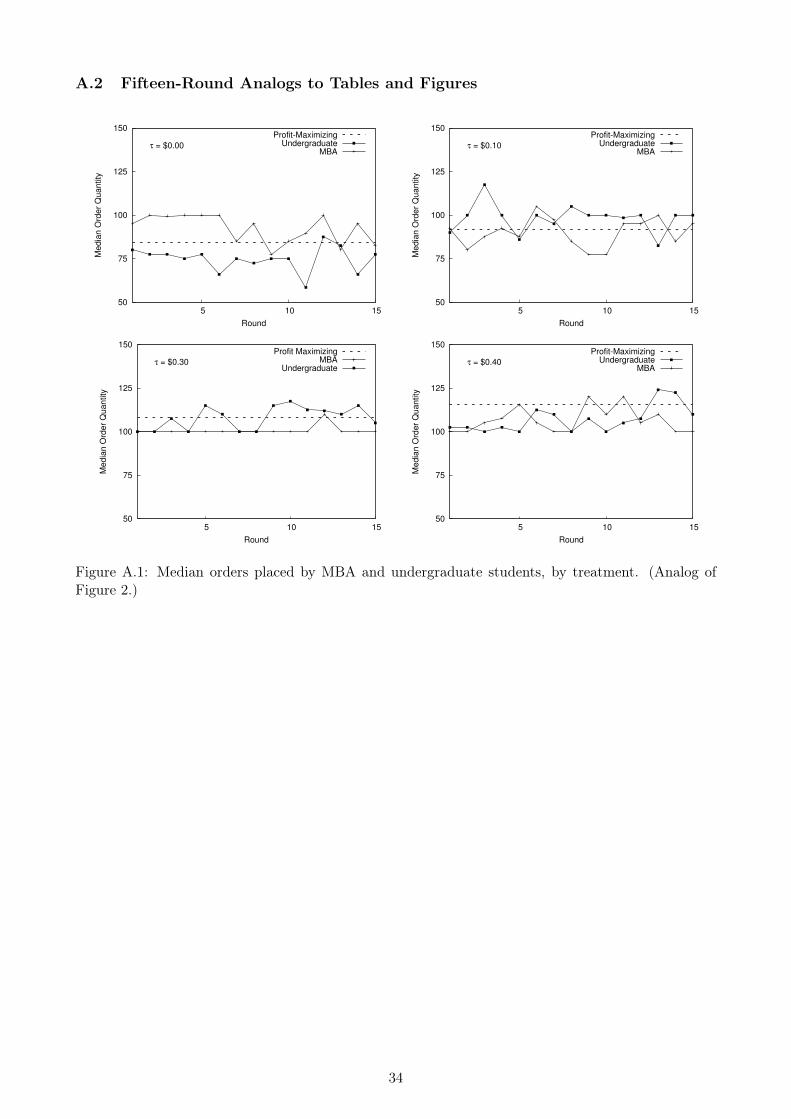
A.2 Fifteen-Round Analogs to Tables and Figures

50

75

100

125

150

5 10 15

Me

dia

n O

rde

r Q

ua

ntity

Round

τ = $0.00

Profit-MaximizingUndergraduate

MBA

50

75

100

125

150

5 10 15

Me

dia

n O

rde

r Q

ua

ntity

Round

τ = $0.10

Profit-MaximizingUndergraduate

MBA

50

75

100

125

150

5 10 15

Me

dia

n O

rde

r Q

ua

ntity

Round

τ = $0.30

Profit MaximizingMBA

Undergraduate

50

75

100

125

150

5 10 15

Me

dia

n O

rde

r Q

ua

ntity

Round

τ = $0.40

Profit-MaximizingUndergraduate

MBA

Figure A.1: Median orders placed by MBA and undergraduate students, by treatment. (Analog ofFigure 2.)

34

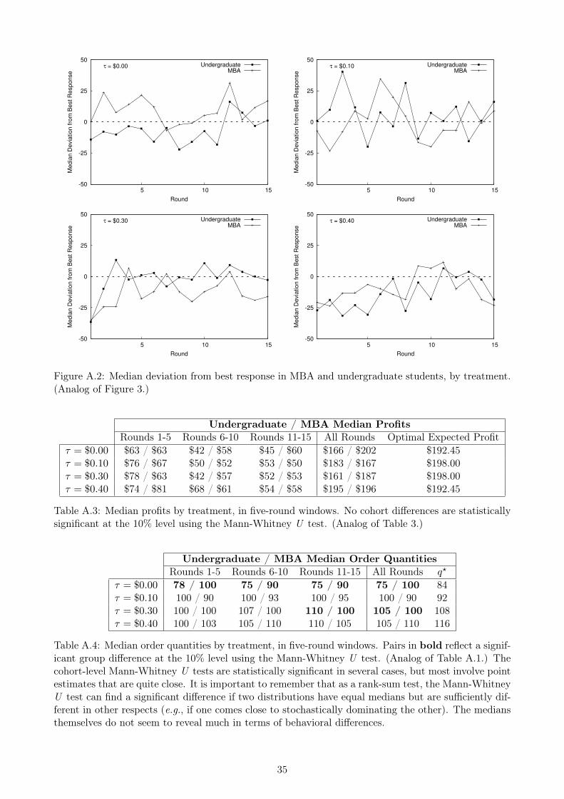
-50

-25

0

25

50

5 10 15

Me

dia

n D

evia

tio

n f

rom

Be

st

Re

sp

on

se

Round

τ = $0.00 UndergraduateMBA

-50

-25

0

25

50

5 10 15

Me

dia

n D

evia

tio

n f

rom

Be

st

Re

sp

on

se

Round

τ = $0.10 UndergraduateMBA

-50

-25

0

25

50

5 10 15

Me

dia

n D

evia

tio

n f

rom

Be

st

Re

sp

on

se

Round

τ = $0.30 UndergraduateMBA

-50

-25

0

25

50

5 10 15

Me

dia

n D

evia

tio

n f

rom

Be

st

Re

sp

on

se

Round

τ = $0.40 UndergraduateMBA

Figure A.2: Median deviation from best response in MBA and undergraduate students, by treatment.(Analog of Figure 3.)

Undergraduate / MBA Median ProfitsRounds 1-5 Rounds 6-10 Rounds 11-15 All Rounds Optimal Expected Profit

τ = $0.00 $63 / $63 $42 / $58 $45 / $60 $166 / $202 $192.45τ = $0.10 $76 / $67 $50 / $52 $53 / $50 $183 / $167 $198.00τ = $0.30 $78 / $63 $42 / $57 $52 / $53 $161 / $187 $198.00τ = $0.40 $74 / $81 $68 / $61 $54 / $58 $195 / $196 $192.45

Table A.3: Median profits by treatment, in five-round windows. No cohort differences are statisticallysignificant at the 10% level using the Mann-Whitney U test. (Analog of Table 3.)

Undergraduate / MBA Median Order QuantitiesRounds 1-5 Rounds 6-10 Rounds 11-15 All Rounds q?

τ = $0.00 78 / 100 75 / 90 75 / 90 75 / 100 84τ = $0.10 100 / 90 100 / 93 100 / 95 100 / 90 92τ = $0.30 100 / 100 107 / 100 110 / 100 105 / 100 108τ = $0.40 100 / 103 105 / 110 110 / 105 105 / 110 116

Table A.4: Median order quantities by treatment, in five-round windows. Pairs in bold reflect a signif-icant group difference at the 10% level using the Mann-Whitney U test. (Analog of Table A.1.) Thecohort-level Mann-Whitney U tests are statistically significant in several cases, but most involve pointestimates that are quite close. It is important to remember that as a rank-sum test, the Mann-WhitneyU test can find a significant difference if two distributions have equal medians but are sufficiently dif-ferent in other respects (e.g., if one comes close to stochastically dominating the other). The mediansthemselves do not seem to reveal much in terms of behavioral differences.

35

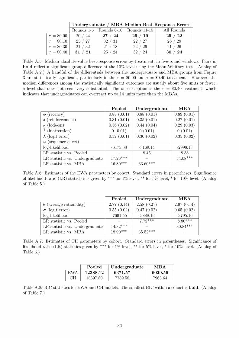
Undergraduate / MBA Median Best-Response ErrorsRounds 1-5 Rounds 6-10 Rounds 11-15 All Rounds

τ = $0.00 20 / 24 27 / 24 25 / 19 25 / 22τ = $0.10 25 / 27 32 / 31 22 / 27 26 / 29τ = $0.30 21 / 32 21 / 18 22 / 29 21 / 26τ = $0.40 31 / 21 25 / 24 32 / 24 30 / 24

Table A.5: Median absolute-value best-response errors by treatment, in five-round windows. Pairs inbold reflect a significant group difference at the 10% level using the Mann-Whitney test. (Analog ofTable A.2.) A handful of the differentials between the undergraduate and MBA groups from Figure3 are statistically significant, particularly in the τ = $0.00 and τ = $0.40 treatments. However, themedian differences among the statistically significant outcomes are usually about five units or fewer,a level that does not seem very substantial. The one exception is the τ = $0.40 treatment, whichindicates that undergraduates can overreact up to 14 units more than the MBAs.

Pooled Undergraduate MBAφ (recency) 0.88 (0.01) 0.88 (0.01) 0.89 (0.01)δ (reinforcement) 0.31 (0.01) 0.35 (0.01) 0.27 (0.01)κ (lock-on) 0.36 (0.02) 0.44 (0.04) 0.29 (0.03)λ (inattention) 0 (0.01) 0 (0.01) 0 (0.01)λ (logit error) 0.32 (0.01) 0.30 (0.02) 0.35 (0.02)ψ (sequence effect) – – –log-likelihood -6175.68 -3169.14 -2998.13LR statistic vs. Pooled – 8.46 8.38LR statistic vs. Undergraduate 17.26*** – 34.08***LR statistic vs. MBA 16.80*** 33.60*** –

Table A.6: Estimates of the EWA parameters by cohort. Standard errors in parentheses. Significanceof likelihood-ratio (LR) statistics is given by *** for 1% level, ** for 5% level, * for 10% level. (Analogof Table 5.)

Pooled Undergraduate MBAθ (average rationality) 2.77 (0.14) 2.58 (0.27) 2.97 (0.14)σ (logit error) 0.55 (0.02) 0.47 (0.02) 0.65 (0.02)log-likelihood -7691.55 -3888.13 -3795.16LR statistic vs. Pooled – 7.72*** 8.80***LR statistic vs. Undergraduate 14.32*** – 30.84***LR statistic vs. MBA 18.90*** 35.52*** –

Table A.7: Estimates of CH parameters by cohort. Standard errors in parentheses. Significance oflikelihood-ratio (LR) statistics given by *** for 1% level, ** for 5% level, * for 10% level. (Analog ofTable 6.)

Pooled Undergraduate MBAEWA 12388.12 6371.57 6029.56CH 15397.80 7789.58 7963.64

Table A.8: BIC statistics for EWA and CH models. The smallest BIC within a cohort is bold. (Analogof Table 7.)

36

Pooled Undergraduate MBAα′ (EWA proportion) 0.96 (0.02) 0.97 (0.06) 0.95 (0.04)φ (recency) 0.87 (0.01) 0.88 (0.01) 0.89 (0.01)δ (reinforcement) 0.30 (0.01) 0.37 (0.01) 0.26 (0.01)κ (lock-on) 0.38 (0.03) 0.44 (0.04) 0.30 (0.03)λ (inattention) 0 (0.01) 0 (0.01) 0.00 (0.01)λ (EWA logit error) 0.32 (0.01) 0.31 (0.02) 0.34 (0.02)ψ (sequence effect) – – –θ (average rationality) 3.81 (1.72) 3.12 (1041) 3.95 (17.75)σ (CH logit error) 6.69 (4.10) 0.18 (1.35) 3.94 (0.96)log-likelihood -6159.12 -3164.25 -2988.37LR statistic vs. Pooled – 4.32 8.66LR statistic vs. Undergraduate 44.20*** – 31.26***LR statistic vs. MBA 8.66 32.80*** –

Table A.9: Estimates of mixture EWA/CH model parameters by cohort. Standard errors in parenthe-ses. Significance of likelihood-ratio (LR) statistics given by *** for 1% level, ** for 5% level, * for 10%level. (Analog of Table 8.)

A.3 EWA and CH Simulations

In Figure A.3, we provide some graphical comparative-static numerical simulations for the modified

EWA model for τ = $0.00 and $0.40. In these exercises, one behavioral parameter is varied while the

others are held at their “most rational” values: φ = 1, δ = 1, κ = 0, λ → ∞, and λ → ∞. Each

exercise consists of 5,000 simulated pairs playing for 15 rounds. In each simulated round, five pieces

of data are generated: two demands x1 and x2 (drawn from the uniform demand distribution), two

choices q1 and q2 (drawn from the probability distributions defined by (11) up to that point), and the

transshipment quantity y1 implied by these draws. We omit the κ simulation because lock-on exhibits

less-pronounced effects at the aggregate level.

37

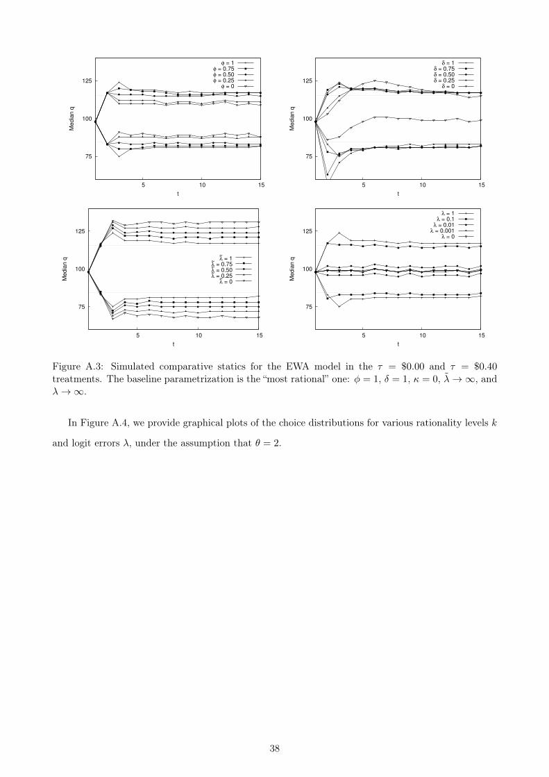
75

100

125

5 10 15

Me

dia

n q

t

φ = 1φ = 0.75φ = 0.50φ = 0.25

φ = 0

75

100

125

5 10 15

Me

dia

n q

t

δ = 1δ = 0.75δ = 0.50δ = 0.25

δ = 0

75

100

125

5 10 15

Me

dia

n q

t

λ~

= 1λ~

= 0.75λ~

= 0.50λ~

= 0.25λ~

= 0

75

100

125

5 10 15

Me

dia

n q

t

λ = 1λ = 0.1

λ = 0.01λ = 0.001

λ = 0

Figure A.3: Simulated comparative statics for the EWA model in the τ = $0.00 and τ = $0.40treatments. The baseline parametrization is the “most rational” one: φ = 1, δ = 1, κ = 0, λ→∞, andλ→∞.

In Figure A.4, we provide graphical plots of the choice distributions for various rationality levels k

and logit errors λ, under the assumption that θ = 2.

38

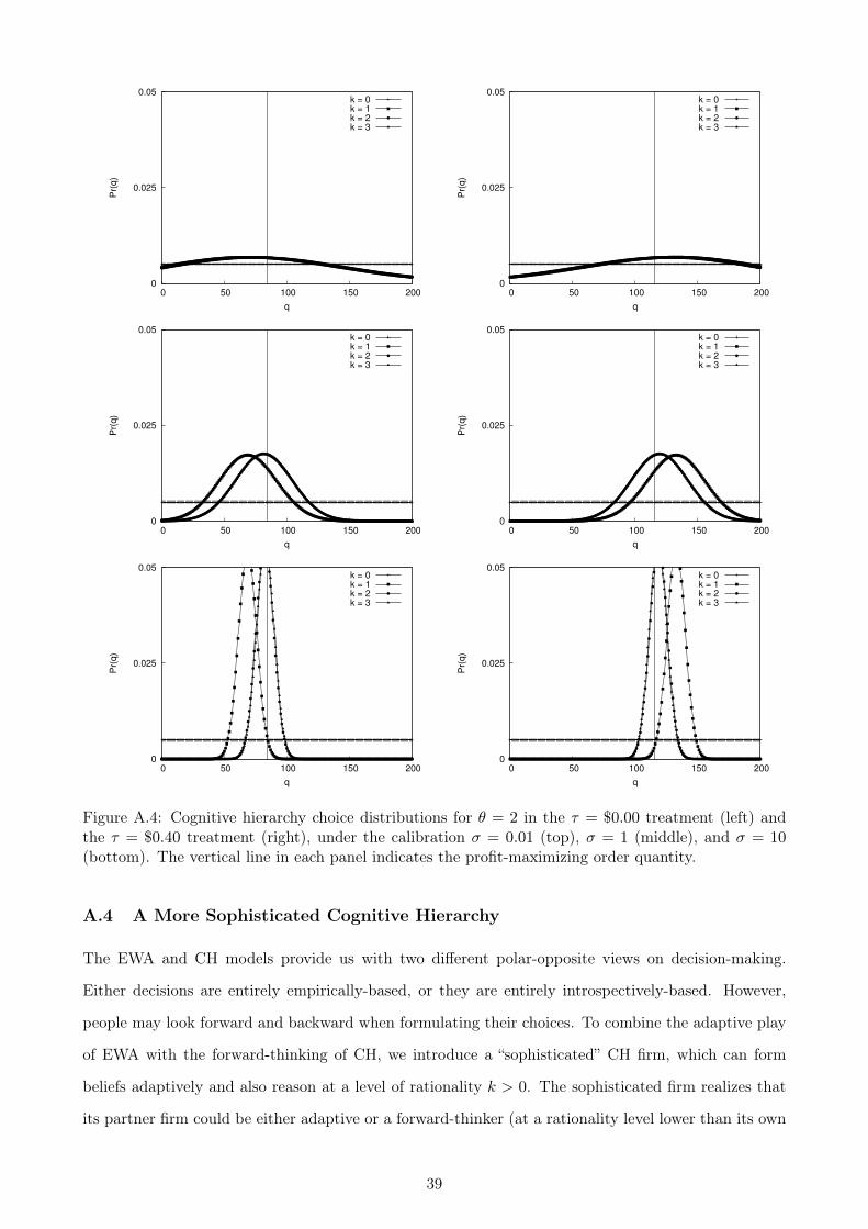
0

0.025

0.05

0 50 100 150 200

Pr(

q)

q

k = 0k = 1k = 2k = 3

0

0.025

0.05

0 50 100 150 200

Pr(

q)

q

k = 0k = 1k = 2k = 3

0

0.025

0.05

0 50 100 150 200

Pr(

q)

q

k = 0k = 1k = 2k = 3

0

0.025

0.05

0 50 100 150 200

Pr(

q)

q

k = 0k = 1k = 2k = 3

0

0.025

0.05

0 50 100 150 200

Pr(

q)

q

k = 0k = 1k = 2k = 3

0

0.025

0.05

0 50 100 150 200

Pr(

q)

q

k = 0k = 1k = 2k = 3

Figure A.4: Cognitive hierarchy choice distributions for θ = 2 in the τ = $0.00 treatment (left) andthe τ = $0.40 treatment (right), under the calibration σ = 0.01 (top), σ = 1 (middle), and σ = 10(bottom). The vertical line in each panel indicates the profit-maximizing order quantity.

A.4 A More Sophisticated Cognitive Hierarchy

The EWA and CH models provide us with two different polar-opposite views on decision-making.

Either decisions are entirely empirically-based, or they are entirely introspectively-based. However,

people may look forward and backward when formulating their choices. To combine the adaptive play

of EWA with the forward-thinking of CH, we introduce a “sophisticated” CH firm, which can form

beliefs adaptively and also reason at a level of rationality k > 0. The sophisticated firm realizes that

its partner firm could be either adaptive or a forward-thinker (at a rationality level lower than its own

39

level). The sophisticated firm then adjusts its behavior to the possibility of its partner being of either

type.

We place a few restrictions on the behavior of a sophisticated CH firm. First, it cannot have a level-0

(pure noise) strategy. The intent of sophistication is to describe a decision process that simultaneously

incorporates adaptive and introspective belief formation, and allowing the level-0 strategy would defeat

that purpose. Because level 0 is excluded, the sophisticated CH model does not precisely nest the CH

model, even if the adaptive part is removed entirely.

Second, a sophisticated CH firm does not assume that its partner is similarly sophisticated. If Firm

1 is sophisticated and also believes that Firm 2 is sophisticated, Firm 1 will need to best-respond to

Firm 2’s sophistication level. Because Firm 1 starts the interaction with no information about Firm 2

at all, Firm 1’s belief about Firm 2’s sophistication level will need to be learned over time. To form

such a complex belief, Firm 1 would need to observe Firm 2’s decisions and outcomes, which this is

not possible in our experimental design.

Because a sophisticated CH firm best-responds to the fact that its partner may be adaptive, its

own decisions will also appear to be correlated with the outcome history. Hence, a sophisticated CH

firm could potentially generate data in line with the stylized facts, without requiring that it actually

be adaptive.

A sophisticated Firm 1 assumes that Firm 2 is adaptive with probability α, and forward-thinking

with probability 1−α. As a result, Firm 1’s beliefs about Firm 2’s likely choices in round t are given by

a weighted average of the EWA belief probabilities from equation (9), and the CH belief probabilities

from equation (12):

Pr (q2t = j|x1t, y1t, r1 = k) = αPr (q2t = j|y1t) + (1− α) Pr (q2t = j|r1 = k)

The expected profits to a sophisticated Firm 1 are

E [π1 (j|x1t, y1t, r1 = k)] =∑m

Ex1,x2 [π1 (j|q2t = m)] Pr (q2t = m|x1t, y1t, r1 = k)

and these translate into logit choice probabilities for Firm 1 in the same manner as before:

Pr (q1t = j|x1t, y1t, r1 = k) =exp (σE [π1 (j|x1t, y1t, r1 = k)])∑m exp (σE [π1 (j|x1t, y1t, r1 = k)])

(13)

As α → 0, the sophisticated belief probabilities become more reflective of a CH best-response, while

they become more reflective of an EWA best-response as α → 1. Note that we use the same logit

parameter σ from the CH part of the belief structure. Because the CH probabilities and those in

40

equation (13) are on the same scale (i.e., expected profits on a narrowly bounded interval), it seems

reasonable that the firm’s sensitivity to profit differences should be similar in both places.

In Figure A.5, we present a comparative-static simulation of α in the τ = $0.00 and τ = $0.40 se-

tups. These exercises are not very revealing unless some bias is present, so we set a baseline parametriza-

tion of φ = 0.75, κ = 0.1, λ = 0.1, θ = 2, σ = 1, and k = 2. (Recall that δ and λ are not relevant to

the formation of EWA belief probabilities, only the choice probabilities.) In this baseline, the median

belief trajectory about an adaptive firm begins at the center of the demand distribution and converges

to the optimal order quantities: from above in the τ = $0.00 case, and from below in the τ = $0.40

case. The mode of the belief distribution about a CH firm converges to the optimal order quantity

from the opposite directions as the rationality level increases.

The simulations show that as α increases (i.e., as Firm 1 believes Firm 2 is more adaptive), a

sophisticated Firm 1 orders increasingly more than the optimum in the τ = $0.40 case and increasingly

less than the optimum in the τ = $0.00 case. This pattern arises because Firm 1 believes that the

adaptive Firm 2 is consistently ordering too little and too much in these respective cases. However,

Firm 1 also believes that Firm 2’s bias dissipates over time as it learns, and so Firm 1’s reaction

mitigates over time as well. Also, as α falls to 0, Firm 1’s median choice becomes only very slightly

biased. In this case, the bias arises from Firm 1’s belief that Firm 2 has a lower rationality level in the

cognitive hierarchy.

Table A.10 presents estimates of this specification. We find again the usual pattern of rejecting

hypotheses of cross-cohort parameter equality. The CH parameters indicate that subjects take about

three steps of mental best response. The adaptive parameters, particularly κ and λ, are poorly iden-

tified, and the estimated probabilities of the partner’s being adaptive are small (from 0.08 to 0.35).

The adaptive part of the model tends to have very high lock-on rates, very low inattention rates,

and sometimes also low recency bias. This is the profile of an “adaptive” player that is settling on a

decision-making strategy extremely quickly, which is almost observationally indistinguishable from the

decisions of a regular forward-thinker.

The BIC statistics for the EWA, CH, and Sophisticated CH models are presented in Table A.11.

In the undergraduate cohort, the BIC statistic favors the more parsimonious CH model over the

sophisticated CH model. In the pooled and MBA cohorts, the Sophisticated CH model represents an

improvement over the regular CH model, but this shift is minor compared to the improvement provided

by EWA explanation. The best explanation of the model appears to be pure adaptivity, and not more

sophisticated reasoning.

41

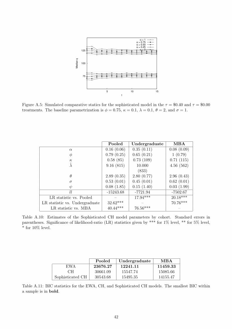
75

100

125

5 10 15

Me

dia

n q

t

α = 1α = 0.75α = 0.50α = 0.25

α = 0

Figure A.5: Simulated comparative statics for the sophisticated model in the τ = $0.40 and τ = $0.00treatments. The baseline parametrization is φ = 0.75, κ = 0.1, λ = 0.1, θ = 2, and σ = 1.

Pooled Undergraduate MBAα 0.16 (0.06) 0.35 (0.11) 0.08 (0.09)φ 0.79 (0.25) 0.65 (0.21) 1 (0.79)κ 0.58 (85) 0.73 (109) 0.71 (115)λ 9.16 (815) 10.000

(833)4.56 (562)

θ 2.89 (0.35) 2.80 (0.77) 2.96 (0.43)σ 0.53 (0.01) 0.45 (0.01) 0.62 (0.01)ψ 0.08 (1.85) 0.15 (1.40) 0.03 (1.99)ll -15243.68 -7721.94 -7502.67

LR statistic vs. Pooled – 17.94*** 20.18***LR statistic vs. Undergraduate 32.62*** – 70.76***

LR statistic vs. MBA 40.44*** 76.56*** –

Table A.10: Estimates of the Sophisticated CH model parameters by cohort. Standard errors inparentheses. Significance of likelihood-ratio (LR) statistics given by *** for 1% level, ** for 5% level,* for 10% level.

Pooled Undergraduate MBAEWA 23676.27 12241.11 11459.33CH 30661.09 15547.74 15085.66

Sophisticated CH 30543.68 15495.35 14155.47

Table A.11: BIC statistics for the EWA, CH, and Sophisticated CH models. The smallest BIC withina sample is in bold.

42

A.5 Individual CH Estimates

Cohort Undergraduate MBAStatistic Median St. Dev. Min Max Median St. Dev. Min Max

θ 3.032 0.819 0.167 4.235 3.234 0.830 0 4.214σ 0.581 1.736 0 8.818 1.003 1.778 0.113 10.000

Table A.12: Summary statistics of individual CH estimates within the experimental cohort.

43