coordinating risk pooling capacity investments in joint...

Submitted tomanuscript

Coordinating Risk Pooling Capacity Investments inJoint Ventures

Philippe ChevalierCORE, Catholic University of Louvain, B-1348 Louvain-la-Neuve, Belgium, [email protected]

Guillaume RoelsUCLA Anderson School of Management, 110 Westwood Plaza, Los Angeles, CA 90095, USA, [email protected]

Ying WeiCORE, Catholic University of Louvain, B-1348 Louvain-la-Neuve, Belgium, [email protected]

Despite their recent proliferation, joint ventures remain challenging to manage when their founding partnershave disparate interests. In this paper we study how to structure a joint-venture contract between twofirms so as to align their incentives to pool together their resources and hedge their profits against demandvariability. We propose two contractual arrangements that lease the capacity of the joint venture to thepartners either in proportion to their respective capacity usages (Total Capacity Leasing) or only to eliminatelocal capacity imbalances (Partial Capacity Leasing). We study when these contracts coordinate the firms’capacity investments and production decisions while ensuring their participation to the joint venture, and wecharacterize the structure of the equilibrium capacity investments. Based on our analysis, we offer contractualrecommendations for coordinating risk-pooling capacity investments as a function of the characteristics ofthe joint venture.

Key words : supply contracts, joint ventures, game theory, newsvendor model, risk poolingHistory : January 26, 2011.

1. IntroductionJoint ventures (JV) and strategic alliances have recently proliferated as a way to enable firmsto manage risk in uncertain markets, share the costs of large-scale projects, or inject new-found entrepreneurial spirit into maturing businesses. Despite their recent proliferation, managingalliances has remained a challenging endeavor. In fact, more than half of the JVs have been reportedto ultimately fail (Bamford et al. 2004). Bamford et al. (2004) argue that most JV failures couldhave been prevented had more time been spent upfront, in the launch phase, to better align thepartners’ strategic objectives, develop a clear governance structure, build a coherent organization,and fully leverage the JV’s operational synergies.

In this paper, we study the strategic interactions that arise in a JV between two manufacturingfirms that decide to pool their resources so as to hedge their profits against demand variability.We consider a situation in which the firms must invest in capacity without actual knowledge of thedemand, i.e., operate as newsvendors. Although there exists a wide variety of reasons for settingup a JV, such as leveraging economies of scale, reinforcing a competitive position, or developingjoint organizational learning (Kogut 1988), we consider here an extreme case in which the firms’rationale for developing the JV is to reduce their total investment costs by leveraging the riskpooling effect across their respective demands.

Our study was motivated by the following four examples of JVs. Our first example is Spairliners,a 50/50 JV between Air France and Lufthansa airlines, created to provide spare part support forAirbus A380 operators. The company established a central pool of components (about 1,100 SKUs)held in two or three key regions (Flight Daily News 2007). Failed or time-expired components are

1

Chevalier, Roels, and Wei: Coordinating Risk Pooling Capacity Investments in Joint Ventures2 Article submitted to ; manuscript no.

exchanged one-for-one, passed back to the Air France and Lufthansa Technic Maintenance andRepair Operations (MRO) centers, and then returned to the pool for subsequent use. Spairlinersnegotiates different tariffs with its customers (i.e., Qantas’s six A380s, Air France’s two A380s, andLufthansa’s three A380s), being typically paid on a power-by-the-hour basis. On the other hand,it must pay its parent companies for the services they perform in their MRO centers (Flight DailyNews 2007).

As a second example, consider the $77.4 million award of the Department of Health and HumanServices (HHS) to Sanofi Pasteur, the largest flu vaccine manufacturer in the US, complementingSanofi’s own $25 million investment to retrofit its existing facilities (Roos 2007). If there is noinfluenza pandemic, Sanofi Pasteur can use its retrofitted production facility at no charge; in caseof influenza outbreak, however, Sanofi must switch to pandemic influenza vaccine manufacture atthe HHS’s request. Hence, similar to Spairliners, Sanofi offers different priorities at different prices.1

Our third example is the Sevel Nord alliance, which was created in 1988 to enable PSA andFiat to jointly enter the multi-purpose vehicle (MPV) market by jointly investing $1 billion inthe design, development, and testing of a new MPV model and $1.2 billion in an entirely newfactory dedicated to this vehicle (Jolly 1997). The alliance was essentially motivated by economiesof scale, because of the small volumes associated with the MPV niche market, and offered veryfew learning opportunities (Jolly 1997). Although the jointly developed MPV was sold under fourdifferent brands (namely, Peugeot 806, Citroen Evasion, Fiat Ulysse and Lancia Zeta) through eachpartner’s respective distribution network,2 the four models were in fact virtually identical–only thefront grill and taillights being unique to each make.

The financial agreement was based on parity: PSA and Fiat equally shared the development andcapital costs and each owned 50% of the JV. Moreover, the Sevel-Nord plant’s capacity was evenlysplit between PSA and Fiat (Jolly 1997). Both partners paid the same per-vehicle purchase priceto the JV, based on a cost-plus formula (Bidault and Schweinsberg 1996). However, if a partner didnot order up to its 50% share of capacity, it could try to sell any portion of the remaining capacityto the other partner. The Sevel-Nord alliance thus offered important opportunities for risk poolingin addition to sharing the fixed development costs.

Our final example is Inotera Memories, a 50/50 JV between Micron and Nanya Technology thatprovides commodity DRAM foundry services on 300mm silicon wafers. Similar to the Sevel-Nordalliance, Inotera’s manufacturing capacity is evenly split between its two customers. However, theper-unit price is based on a margin-sharing principle, i.e., sharing the “profit (or loss) realized onthe sale of the good chips on [the] wafers” (Inotera 2009).

Although these four JVs leverage risk pooling and economies of scale, the contractual arrange-ments appear to be significantly different. Whereas the joint capacity of Sevel-Nord and Inotera isevenly split between the parent companies, with potential capacity transfers, Sanofi Pasteur offers apreemption right to the HHS. The pricing schemes also differ, ranging from cost-plus (Sevel-Nord)and margin-sharing (Inotera) to pure differentiated pricing (Spairliners, Sanofi Pasteur). Is thereany commonality among those contracts? Under what conditions do those contracts coordinate thepartners’ capacity investments and their production planning decisions? Which type of contractfits best which type of JV?

In this paper, we develop two contracting models, namely the total capacity leasing (TCL) con-tract and the partial capacity leasing (PCL) contract, for coordinating the decisions of independentfirms that pool their resources together in an JV. Under the TCL contract, the entire capacity is

1 Although Sanofi can use its facilities at no charge, it seems that it collects a profit margin on the flu vaccines itsells to the HHS. In 2008, the HHS ordered 39 million doses of vaccine from Sanofi at an average unit price of $5(Mcdonald 2008), whereas the variable cost has been estimated to $3 (Deo and Corbett 2009).

2 There was only limited competition between the two car makers given that a large fraction of their sales originatedfrom their respective home markets (Bidault and Schweinsberg 1996).

Chevalier, Roels, and Wei: Coordinating Risk Pooling Capacity Investments in Joint VenturesArticle submitted to ; manuscript no. 3

centrally managed by the JV. Each time a partner uses the pooled resources to meet its demand, itmust pay a leasing fee to the JV proportionally to its production quantity. At the end of the JV’slife, the total fees collected by the JV are shared among the partner firms in proportion to theirrespective capacity investments. By contrast, under the PCL contract, the capacity is indepen-dently managed by its respective buyers and leases occur only partially, in case a partner wishesto purchase extra capacity to satisfy her demand.

We study when those contracts guarantee that (i) the firms agree to invest in the first-best levelof capacity, (ii) the firms agree on the first-best production plan, and (iii) the firms are willing toparticipate to the JV without introducing additional transfer payments. We show that all threerequirements can only be satisfied under TCL contracts when there is a large gap between theproducts’ respective profit margins and when the demand for the least profitable product is suffi-ciently large. By contrast there always exists a PCL contract that satisfies all three requirements.On the other hand, we show that the TCL contract involves a stable negotiation process and canbe easily implemented in more complex environments, with an arbitrary number of partners, prod-ucts, and resources. Our contractual framework therefore helps understand the pros and cons ofeach contract, depending on the JV’s characteristics.

The paper is organized as follows. We review the relevant literature in the next section andintroduce the model in Section 3. Section 4 introduces the TCL contract, proves the existence anduniqueness of a Nash equilibrium in the capacity investment game, characterizes the conditionsunder which full coordination is achieved, shows how the fee parameters can be obtained as theoutcome of an iterative negotiation process, and studies the sensitivity of its parameters to thedegree of demand uncertainty and to the cost parameters. Section 5 then introduces the PCLcontract, proves the existence and uniqueness of a Nash equilibrium in the capacity investmentgame, and characterizes the conditions under which full coordination is achieved. We present ourconclusions in Section 6 and discuss future research directions. All proofs appear in appendix.

2. Literature ReviewThe hybrid nature of JVs has generated a lot of academic research interest, from the perspec-tives of transaction cost economics (Hennart 1988), contract theory (Grossman and Hart 1986),organization theory (Borys and Jemison 1989), and strategic management theory (Harrigan 1988)among others. Following Harrigan’s (1988) JV framework, we consider here a situation of stag-nating demand with high market uncertainty, leading horizontal firms to create a JV so as toconsolidate capacity and benefit from risk pooling.

We first review the literature related to investment in flexible capacity, which explores the invest-ment strategies in the presence of risk pooling opportunities, and then review the literature onsupply chain coordination.

2.1. Investment in Flexible ResourcesThe newsvendor model, which studies the capacity investment decision a firm needs to makewithout knowing demand, lies at the foundation of stochastic inventory theory (Porteus 1990) andis also ubiquitous in capacity investment models (Van Mieghem 2003). In this paper, we study howto coordinate capacity investment decisions between two decentralized newsvendors.

Because of risk pooling, resource flexibility reduces the need to invest in capacity for a targetedservice level. Van Mieghem (1998) characterizes the optimal investment in flexible and dedicatedresources as a function of the product mix and demand correlation. Considering multiple plantsmanufacturing multiple products, Jordan and Graves (1995), Graves and Tomlin (2003), and Bas-samboo et al. (2010) show that almost all benefits of a fully flexible system can be achievedwhen each plant is flexible enough to manufacture just two products, and that flexibility exhibits


decreasing marginal returns. In this paper, we will consider risk pooling as one of the main benefitsassociated with the creation of a JV between independent newsvendors.

Similar to this paper, Van Mieghem (1999) studies two decentralized newsvendors and proposesa contracting framework for coordinating outsourcing and subcontracting decisions. In his model,capacities are installed at each of the newsvendor’s facilities and capacity sharing can only occurin one direction, when one of the newsvendor subcontracts its production to the other newsvendor.In contrast, in our JV model, capacity is pooled and can be used by either of the newsvendors.Van Mieghem (1999) studies the performance of three different types of contracts in terms of theirability to coordinate capacity investment and production decisions. He shows that, in contrast tofixed-price contracts and incomplete contracts, which do not coordinate the capacity investmentdecisions, state-dependent transfer price contracts coordinate both investment and productiondecisions. The latter contract is in fact similar to our PCL contract, except that we consider asituation in which the entire capacity is pooled, allowing for bilateral capacity transfers.

2.2. Supply Chain CoordinationUsing contracts to coordinate decisions in decentralized supply chains has received considerableattention in the past decade. Studying vertical supply chains, Lariviere and Porteus (2001) andCachon and Lariviere (2001) show that price-only contracts do not coordinate the capacity invest-ments because of double marginalization and Perakis and Roels (2007) show that the resultinginefficiencies can be rather substantial. In particular, the risk pooling effect obtained from flexibleresources can be dampened by the strategic interactions among the component suppliers (Bern-stein et al. 2007). To eliminate double marginalization, supply chain partners can adopt “smartercontracts,” such as buy-back contracts, revenue-sharing contracts, or quantity-discount contracts;see Cachon (2003) for a review.

Studying competition in horizontal supply chains, Lippman and McCardle (1997) and Netessineand Rudi (2003) show that competing firms facing uncertain demand, i.e., newsvendors, wouldglobally overinvest in capacity. In their models, the unmet demand of one firm experiencing astockout is “re-allocated” to competing firms according to some mechanism. Anupindi et al. (2001)also consider independent newsvendors, but they allow them to transship their inventories so asto maximize the global ex-post profits, therefore reducing the local mismatches between supplyand demand. In order to ensure participation of all the newsvendors to the ex-post transshipmentprocess, they propose a “dual allocation rule” mechanism, based on the dual solution of the cor-responding transshipment optimization problem. Implementing the dual allocation rule remainshowever challenging as retailers may want to withhold their inventory (Granot and Sosic 2003)or may converge to a suboptimal equilibrium (Suakkaphong and Dror 2009). Instead of havingrecourse to an ex-post allocation rule, Rudi et al. (2001) and Hu et al. (2007) propose to coordi-nate the newsvendor transshipment decisions with ex-ante transshipment prices, in a two-retailerdistribution system. Dong and Rudi (2004) and Krishnan et al. (2010) further study the benefits oftransshipment prices in decentralized distribution networks. Huang and Sosic (2010) compare thetwo mechanisms and show that the dual allocation rule outperforms transshipment prices whenretailers are asymmetric and that the opposite holds when retailers are similar.

Despite their similarities, capacity and inventory sharing cannot be managed in the same waybecause production capacity is inherently more flexible than inventory. In particular, capacity iscompletely undifferentiated before it is used whereas inventory’s usage costs may depend on whobought it and where it is stored. Consequently, with capacity, it may not be optimal to satisfy the“local” demands first before satisfying the excess demand of other products, which is a necessarycondition for the applicability of the dual allocation rule (Suakkaphong and Dror 2009).

Using a cooperative game-theoretic framework, Hartman et al. (2000) and Muller et al. (2002)study how to allocate the gains from centralizing the inventory of multiple newsvendors and avoid


the emergence of subcoalitions. We complement their analysis of the benefits of coalition by adopt-ing a non-cooperative game-theoretic framework to study the strategic interactions, and the result-ing equilibrium investments, associated with the creation of a JV. Indeed, Bamford et al. 2004 stressthe importance of understanding the strategic conflicts upfront and better aligning the partners’interests in the launch phase of the JV. As our analysis will reveal, different contract forms lead todifferent structures of investment. We therefore enrich the cooperative game-theoretic frameworkby shedding light onto the strategic interactions that arise in the capacity investment stage and byestablishing the convergence of the contract negotiation.

3. Decentralized Newsvendor ModelWe model the JV’s operations as a two-period game, akin to the newsvendor model, as it frequentlyoccurs in the high-tech industry and the automotive industry (e.g., Van Mieghem 1999, Anupindiet al. 2001, Cachon and Lariviere 2001). In the first period, the JV partners decide on theirinvestments in a common resource without knowing the demand for their products. In the secondperiod, demand is realized, and the partners choose how to allocate the joint capacity so as tofulfill their respective demands.

For ease of exposition, we consider only two partners, each producing one product, sold on distinctmarkets, and one single flexible production equipment. This simple setting can be interpreted as ahigh-level, “black-box” description of a complex newsvendor network production facility. Althoughour analysis will be based on this simple setting, we shall discuss how the proposed contractualframework can be extended to more complex environments.

In the capacity investment stage, the partners decide on their respective investments, y1 and y2,in order to build the facility with total capacity y = y1 + y2. We assume linear costs of capacity;specifically, let c > 0 be the unit cost of equipment. Although capacity investments are oftenassociated with economies of scale in practice, we shall ignore them in our analysis in order tofocus on the JV partners’ incentive issues that arise from the pooling of resources in the presenceof demand uncertainty. Our results shall accordingly be interpreted as minimal requirements forcoordinating the JV.

After the investment stage, demand is realized. For each product i = 1,2, the demand Di isassumed to have a continuous probability distribution function Fi(ξ) = P[Di ≤ ξ] with support[li, ui), for 0≤ li <ui ≤∞, and expectation E[Di]. Let us also denote Fi(ξ) = 1−Fi(ξ) the comple-mentary distribution of Di, fi(ξ) its density, and hi(ξ) = fi(ξ)/Fi(ξ) its failure rate. As is commonin the supply chain contracting literature (Cachon 2003), we assume that Di has an increasingfailure rate (IFR), which is satisfied by most common distributions (Bagnoli and Bergstrom 2005).Let D=D1 +D2 be the total demand, with support [l, u) = [l1 + l2, u1 +u2), distribution functionF (ξ) = P[D1 + D2 ≤ ξ], complementary distribution F (ξ) = 1 − F (ξ), density f(ξ) = F ′(ξ), andfailure rate h(ξ) = f(ξ)/F (ξ). If D1 and D2 are independent and IFR, the total demand D1 +D2

(i.e., their convolution) is also IFR; moreover, h(ξ)≤min{h1(ξ), h2(ξ)} (Theorems 5.1. and 5.4 inBarlow and Proschan 1965).

Upon observing the demand, the partners must then decide on a joint production plan. Assumingexogenous prices, we denote by vi the gross profit margin associated with product i. Withoutloss of generality, we assume that each unit of product consumes exactly one unit of the flexibleresource and that product 1 has a higher profit margin than product 2, i.e. v1 ≥ v2, with v1 > c. Theproduction plan that maximizes the JV’s ex-post surplus thus consists in allocating all capacityin priority to product 1. Under this optimal production plan, the sales of products 1 and 2 arerespectively equal to x1(y,D1,D2) = min{D1, y} and x2(y,D1,D2) = min{D2, (y−D1)+}, in which(z)+ = max{z,0}. We denote the expected sales by Si(y) = E[xi(y,D1,D2)], the total expected salesby S(y) = S1(y) +S2(y), and the total expected revenue by R(y) = v1S1(y) + v2S2(y).


When all costs and prices are expressed in real terms, the JV’s expected profit, under the optimalproduction plan, can be written as Π(y) =R(y)− cy and is concave (Harrison and Van Mieghem1999). The first-best capacity investment y∗ thus solves the following optimality condition:

v1S′1(y∗) + v2S

′2(y∗) = c. (1)

To simplify the exposition, we assume that the first-best capacity investment is unique, which holdswhen the profit function is strictly concave on its domain of definition, i.e., when (v1− v2)f1(ξ) +v2f(ξ)> 0 for all ξ ∈ [l1, u). In particular, we assume that f1(ξ)> 0 on its support [l1, u1) (whichholds when D1 is IFR, see Lemma 2 in Lariviere and Porteus 2001), that f(ξ)> 0 on its support[l, u) (which holds in particular when D1 +D2 is IFR), that the support of D1 overlaps with thesupport of D1 +D2, i.e., that u1 > l, and that v1 > v2 > 0.

As a benchmark, let us consider the profits the individual firms would have obtained withoutrisk pooling, i.e., as if they had operated as independent newsvendors. For each firm i = 1,2,let SNVi (y) = E[min{y,Di}] be the expected sales without pooling. Each firm i would then haveinvested yNVi to maximize its own profit ΠNV

i (y) = viSNVi (y)−cy. Because the JV’s profit is globally

optimized, we obviously have that Π(y∗)≥ΠNV1 (yNV1 ) + ΠNV

2 (yNV2 ), and the effect would even bestronger in the presence of economies of scale.

In the following two sections, we propose two contractual arrangements, namely the TCL andthe PCL contracts, that replicate the system-optimal investment and production decisions underdecentralized decision-making. Unlike profit-sharing contracts, which share the total surplus Π(y∗)in predetermined proportions, those two contractual arrangements lead to a unique Nash equilib-rium in the capacity investment game, and therefore allow for an unambiguous characterizationof the strategic interactions. In their implementation, they only require verifiability of the rela-tive product profitability, the relative investments, and the respective sales, whereas profit sharingcontracts require full information disclosure on profit margins, investments, and demands.

4. Total Capacity Leasing ContractsIn this section, we introduce the TCL contract, which aligns the JV partners’ incentives to sharecapacity and hedge their profits against demand uncertainty through risk pooling. After estab-lishing the existence and uniqueness of a Nash equilibrium in the capacity investment game, wecharacterize the conditions under which this contract coordinates the partners’ investment andproduction decisions, while ensuring their participation to the JV. We also demonstrate the sta-bility of the TCL contract negotiation process and study the sensitivity of the contract fees to thepartners’ characteristics.

Under a TCL contract, the total capacity is managed by the JV and leased to the partners inproportion to their respective capacity usages. Specifically, the TCL contract works as follows:• In the investment stage, each manufacturer i invests yi in the flexible resource at a cost cyi;

the pooled capacity y= y1 + y2 is then managed by the JV.• In the production stage, the quantities that maximize the joint surplus are produced. Each

manufacturer i collects the gross profit associated with its own sales, vixi(y,D1,D2), and pays theJV a leasing fee λi for each unit of capacity used by its own products, λixi(y,D1,D2).• At the end of the production stage, the JV’s total leasing revenue λ1x1(y,D1,D2) +

λ2x2(y,D1,D2) is redistributed to the partners proportionally to their relative capacity investments(y1/y, y2/y).

Accordingly, manufacturer i’s expected profit under a TCL contract is equal to

ΠTCLi (yi;y−i) = (vi−λi)Si(y)− cyi +

yiy

(λ1S1(y) +λ2S2(y)) . (2)


The TCL contract thus resembles the contractual arrangements adopted by Spairliners and SanofiPasteur. Similar to the Spairliners JV, the financial flows under a TCL contract are bidirectional,going from customers (which include the parent companies) to the JV as a function of theircapacity usage (e.g., through the power-by-the-hour contracts) and from the JV to its parents asa function of their relative capacity investments (e.g., through repair and maintenance service feesand dividends). Although capacity rationing seems not to be of primary importance for Spairlinersgiven its high levels of service guarantees (typically between 95% and 98%, see Karp 2006), it liesat the core of the contract between Sanofi and the HHS, which explicitly states that an HHS’s fluvaccine order would preempt the production of Sanofi Pasteur’s regular pharmaceutical products.

Depending on the relative values of the leasing fees (λ1, λ2), the TCL contract can be offeredunder various pricing schemes, such as fixed price (λ1 = λ2), margin sharing (λ1/v1 = λ2/v2), orpreemptive pricing (λ2 = 0 and λ1 > 0).

The TCL contract can be easily extended to more complex environments, with an arbitrarynumber of partners, each operating a newsvendor network with multiple products and multipleresources (Van Mieghem and Rudi 2002). Note that the products could also be directly competingfor the same demand; for instance, with two products, the ex-post production planning problemcould be to maximize v1x1 + v2x2 subject to the capacity constraint x1 + x2 ≤ y and a demandsubstitution constraint, x1 + αx2 ≤ D, for some α ∈ (0,1], as well as nonnegativity constraints,x1, x2 ≥ 0. With N products and K resources, the TCL contract would then require at most NKparameters, by associating a fee to each product/resource pair.

4.1. Existence and Uniqueness of Nash EquilibriumWe next show that there exists a unique Nash equilibrium in the capacity investment game underthe TCL contract. The existence proof, which relies on Debreu-Glicksberg-Fan’s theorem (Fuden-berg and Tirole 1991), requires the manufacturers’ profit functions (2) to be quasiconcave. However,because manufacturer 2 has only access to the leftover capacity and therefore faces both demandand supply uncertainty, its profit function is in general not concave.

It can nevertheless be shown to be quasiconcave under a selected range of contract parameters(λ1, λ2). In particular, we assume that the solution to λ1S1(y) + λ2S2(y) = cy, denoted by y, isgreater than the first-best investment y∗. In that case, the equilibrium investment will lie betweeny∗ and y; that is the the manufacturers will typically overinvest in capacity in equilibrium. Wealso assume that the leasing fee paid by manufacturer 1 is sufficiently large, i.e., λ1 ≥ c/F (y), tomotivate manufacturer 2 to invest in the joint facility, despite the fact that she has only access tothe leftover capacity. Although these conditions are only sufficient to establish the existence of aNash equilibrium, they are always satisfied by all contracts that coordinate the capacity investmentdecisions and the production decisions, as we shall see in §4.2.

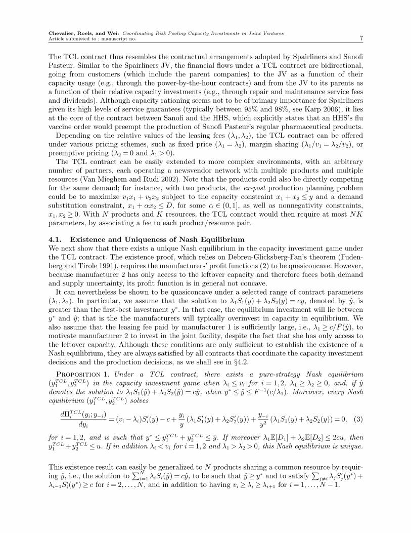
Proposition 1. Under a TCL contract, there exists a pure-strategy Nash equilibrium(yTCL1 , yTCL2 ) in the capacity investment game when λi ≤ vi for i = 1,2, λ1 ≥ λ2 ≥ 0, and, if ydenotes the solution to λ1S1(y) + λ2S2(y) = cy, when y∗ ≤ y ≤ F−1(c/λ1). Moreover, every Nashequilibrium (yTCL1 , yTCL2 ) solves

dΠTCLi (yi;y−i)dyi

= (vi−λi)S′i(y)− c+yiy

(λ1S′1(y) +λ2S

′2(y)) +

y−iy2

(λ1S1(y) +λ2S2(y)) = 0, (3)

for i = 1,2, and is such that y∗ ≤ yTCL1 + yTCL2 ≤ y. If moreover λ1E[D1] + λ2E[D2] ≤ 2cu, thenyTCL1 +yTCL2 ≤ u. If in addition λi < vi for i= 1,2 and λ1 >λ2 > 0, this Nash equilibrium is unique.

This existence result can easily be generalized to N products sharing a common resource by requir-ing y, i.e., the solution to

∑N

i=1 λiSi(y) = cy, to be such that y≥ y∗ and to satisfy∑

j 6=i λjS′j(y∗) +

λi−1S′i(y∗)≥ c for i= 2, . . . ,N , and in addition to having vi ≥ λi ≥ λi+1 for i= 1, . . . ,N − 1.


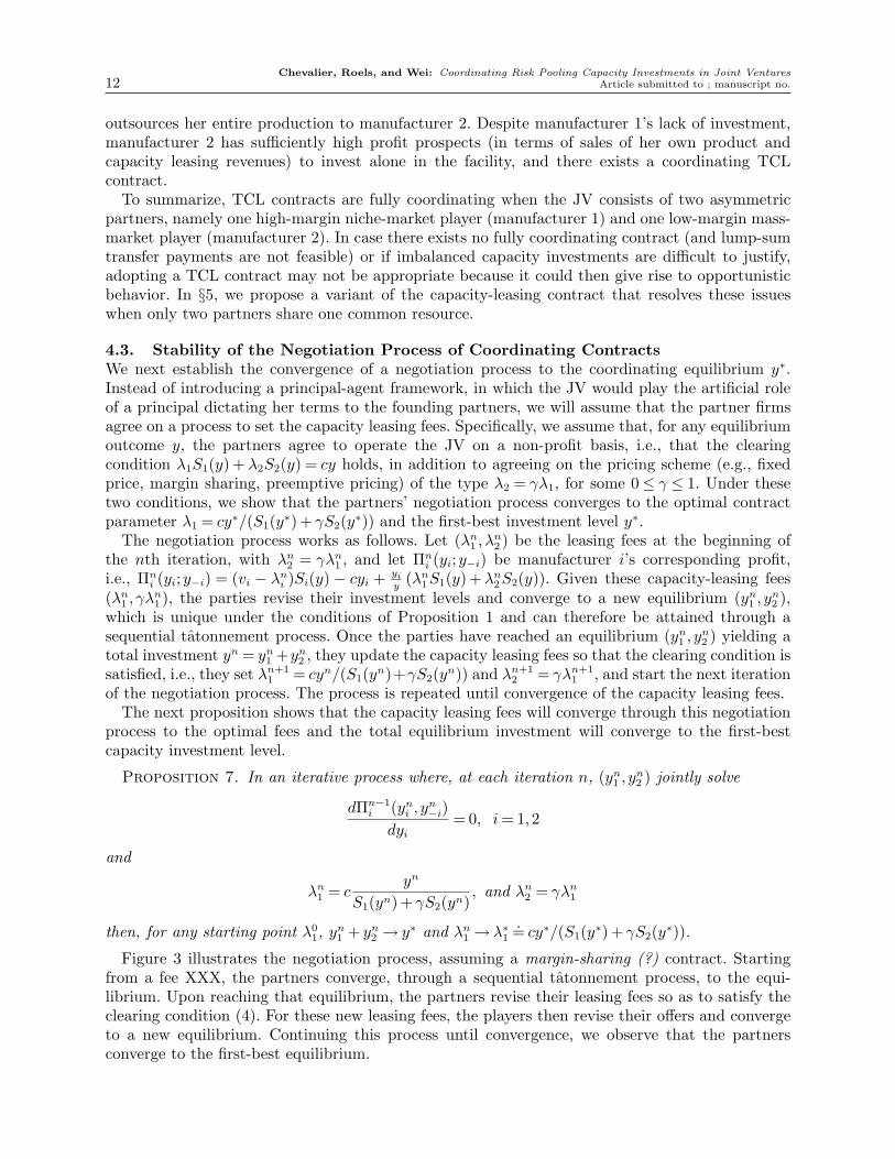
Figure 1 Example of the convergence of the sequential tatonnement process.

As a consequence of the uniqueness, the game is dominance solvable, implying Cournot stability(Vives 2001). That is, for any (λ1, λ2) satisfying the conditions for uniqueness stated in Proposition1, the corresponding Nash equilibrium can be found through a sequential tatonnement process, inwhich the players alternate in taking actions. Figure 1 illustrates this tatonnement process, whenboth players initially start to offer to invest 10 units. After the initial offer, each player in turnrevise its offer based on its best-response curve until they converge to the unique equilibrium.The parameters of this example are v1 = 100, v2 = 40, c = 30, λ1 = 65, λ2 = 25, D1 and D2 areindependent Beta-binomial distributions, both with a mean of 15, and with respective variances of30 and 20.

4.2. Coordinating ContractsWe say that a contract is coordinating if the following properties are satisfied.• A contract is said to make the partners’ investment incentives compatible (ICInv) if the total

equilibrium investment is equal to the first-best investment level.• A contract is said to make the partners’ production incentives compatible (ICProd) if all partners

agree to implement the first-best production plan, for any demand realization. In particular, withone flexible resource and two partners, a contract satisfies the (ICProd) requirement if both partiesalways agree to allocate the capacity in priority to the most profitable product.• A contract is said to satisfy the individual rationality (IR) or participation constraints if each

partner earns individually more under the JV agreement than if it had operated as an independentnewsvendor, that is, if Πi(yi;y−i)≥ΠNV

i (yNVi ). This concern may however be eliminated with thetransfer of lump-sum payments, especially when the creation of the JV is associated with fixedcosts, as it often happens.

We next characterize the conditions under which the TCL contracts are coordinating the invest-ment decisions.

Proposition 2 (ICInv). Under a TCL contract (λ1, λ2), with λ1 >λ2 > 0, the capacity invest-ment Nash equilibrium (yTCL1 , yTCL2 ) is such that yTCL1 + yTCL2 = y∗ if and only if

λ1S1(y∗) +λ2S2(y∗) = cy∗, (4)

and if (4) holds, the equilibrium profits (2) simplify to:

ΠTCLi (yi;y∗− yi) = (vi−λi)Si(y∗). (5)


Hence, the capacity investments are coordinated under the TCL contract if and only if (4)holds. Because the first-best investment y∗ is independent of the contract parameters, Condition(4) actually defines a linear relationship between λ1 and λ2, see Figure 2. Under this condition,the expected leasing revenue collected by the JV is set equal to the investment cost; that is, theJV must operate on a non-profit basis. Similarly, under (4), each player’s investment cost cyi isequal to its expected dividend (yi/y∗)(λ1S1(y∗) +λ2S2(y∗)). This clearing condition is thus similarto the requirement for avoiding double marginalization in vertical supply chains, namely that theprofit margins of all but one partners are set to zero.

Note also that this clearing condition can be generalized to more complex environments with Nproducts, potentially serving the same markets. If there is only one resource to be shared by Nproducts, the clearing condition defines a hyperplane in the space of leasing fees:

∑N

i=1 λiSi(y∗) =

cy∗. With K > 1 resources, one needs to define one clearing condition per resource, leaving (N−1)Kdegrees of freedom to arbitrarily allocate the profits.

By plugging the clearing condition (4) into the equilibrium conditions (3), we obtain that, fori= 1,2, the share of respective investments is equal to

yTCLi

y∗=

(vi−λi)S′i(y∗)c−λ1S′1(y∗)−λ2S′2(y∗)

. (6)

Although the respective investments induced by the coordinating contract are guaranteed to benonnegative when vi ≥ λi, manufacturer 1 will invest nothing in the JV when S′1(y∗) = 0. Thiscondition is in particular satisfied when v2 > c and the demand for product 2 is so large thaty∗ > u1. In that case, manufacturer 1 effectively outsources her production to manufacturer 2without owning a stake in the facility, such as when Volkswagen outsourced its production of low-volume Routan minivans to Chrysler, on the same line as Chrysler’s large-volume Dodge Caravanminivans (Benett 2008).

From (5) and (6), we obtain that yTCL1 /yTCL2 = (v1 − λ1)/(v2 − λ2)(S′1(y∗)/S′2(y∗)) =ΠTCL

1 /ΠTCL2 (S′1(y∗)S2(y∗))/(S1(y∗)S′2(y∗)), that is, the investment split is directly proportional to

the profit split. The next proposition characterizes the sensitivity of the equilibrium investmentsand profits to the capacity leasing fees of a coordinating TCL contract. We find that a manufac-turer’s equilibrium investment and profit are naturally decreasing in her own capacity-leasing feeand increasing in her partner’s fee. Along the coordinating line (4) (see Figure 2), different pairs ofleasing fees (λ1, λ2) therefore correspond to different profit allocations of the total JV profit Π(y∗)and different investment splits of y∗.

Moreover, we find that, provided yNV1 h(yNV1 )≥ 1, manufacturer 1’s investment is decreasing inv2, for any given pricing scheme. Note that the condition yNV1 h(yNV1 )≥ 1, even though it is onlysufficient, naturally holds when manufacturer 1 has a high profit margin v1/c, given that yh(y) isincreasing.

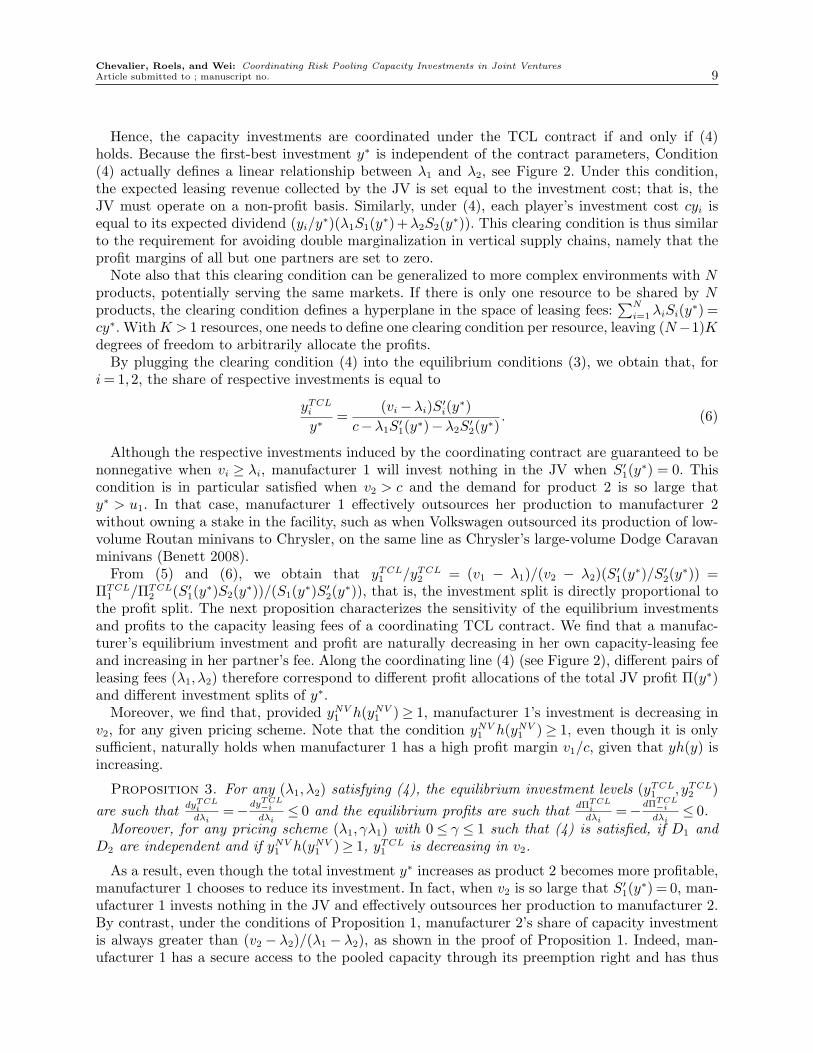
Proposition 3. For any (λ1, λ2) satisfying (4), the equilibrium investment levels (yTCL1 , yTCL2 )are such that dyTCLi

dλi=−dyTCL−i

dλi≤ 0 and the equilibrium profits are such that dΠTCLi

dλi=−dΠTCL−i

dλi≤ 0.

Moreover, for any pricing scheme (λ1, γλ1) with 0≤ γ ≤ 1 such that (4) is satisfied, if D1 andD2 are independent and if yNV1 h(yNV1 )≥ 1, yTCL1 is decreasing in v2.

As a result, even though the total investment y∗ increases as product 2 becomes more profitable,manufacturer 1 chooses to reduce its investment. In fact, when v2 is so large that S′1(y∗) = 0, man-ufacturer 1 invests nothing in the JV and effectively outsources her production to manufacturer 2.By contrast, under the conditions of Proposition 1, manufacturer 2’s share of capacity investmentis always greater than (v2 − λ2)/(λ1 − λ2), as shown in the proof of Proposition 1. Indeed, man-ufacturer 1 has a secure access to the pooled capacity through its preemption right and has thus


very little incentive to invest in capacity. By contrast, manufacturer 2, because it has only accessto the leftover capacity, has a strong incentive to invest in capacity if she wants to sell anything.The TCL contract thus leads to a relatively imbalanced structure of investments, in which themost profitable manufacturer essentially relies on the other manufacturer’s capacity investment byinvesting marginally while enjoying a preemption right on the joint resource.

The next proposition characterizes the conditions under which the TCL contract coordinatesthe production planning decisions, in the presence of a single resource. With multiple resources,there exists in general no TCL contract that could satisfy (ICProd), unless the prioritization orderis independent of the demand, as it arises, for instance, with one flexible resource and multiplededicated resources, similar to Van Mieghem’s (1999) model.

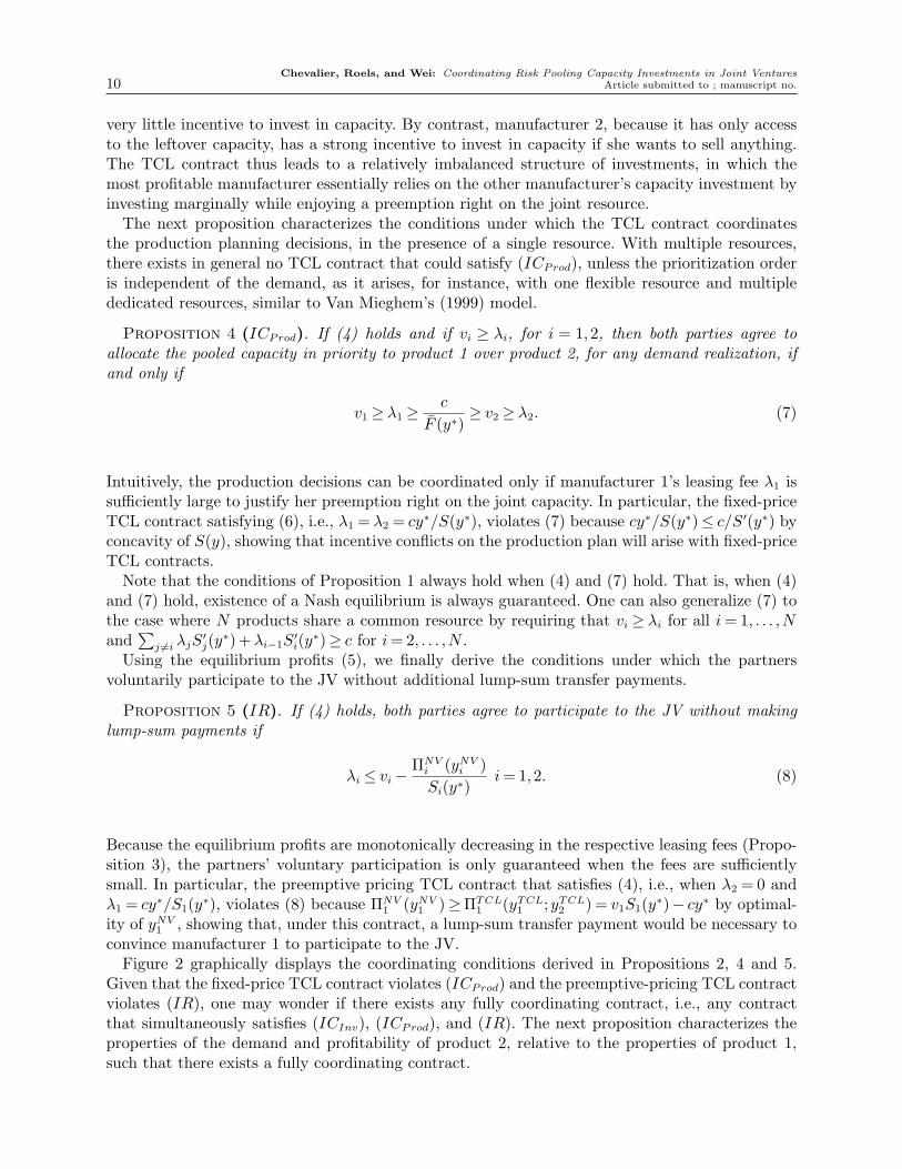
Proposition 4 (ICProd). If (4) holds and if vi ≥ λi, for i = 1,2, then both parties agree toallocate the pooled capacity in priority to product 1 over product 2, for any demand realization, ifand only if

v1 ≥ λ1 ≥c

F (y∗)≥ v2 ≥ λ2. (7)

Intuitively, the production decisions can be coordinated only if manufacturer 1’s leasing fee λ1 issufficiently large to justify her preemption right on the joint capacity. In particular, the fixed-priceTCL contract satisfying (6), i.e., λ1 = λ2 = cy∗/S(y∗), violates (7) because cy∗/S(y∗)≤ c/S′(y∗) byconcavity of S(y), showing that incentive conflicts on the production plan will arise with fixed-priceTCL contracts.

Note that the conditions of Proposition 1 always hold when (4) and (7) hold. That is, when (4)and (7) hold, existence of a Nash equilibrium is always guaranteed. One can also generalize (7) tothe case where N products share a common resource by requiring that vi ≥ λi for all i= 1, . . . ,Nand

∑j 6=i λjS

′j(y∗) +λi−1S

′i(y∗)≥ c for i= 2, . . . ,N .

Using the equilibrium profits (5), we finally derive the conditions under which the partnersvoluntarily participate to the JV without additional lump-sum transfer payments.

Proposition 5 (IR). If (4) holds, both parties agree to participate to the JV without makinglump-sum payments if

λi ≤ vi−ΠNVi (yNVi )Si(y∗)

i= 1,2. (8)

Because the equilibrium profits are monotonically decreasing in the respective leasing fees (Propo-sition 3), the partners’ voluntary participation is only guaranteed when the fees are sufficientlysmall. In particular, the preemptive pricing TCL contract that satisfies (4), i.e., when λ2 = 0 andλ1 = cy∗/S1(y∗), violates (8) because ΠNV

1 (yNV1 )≥ΠTCL1 (yTCL1 ;yTCL2 ) = v1S1(y∗)− cy∗ by optimal-

ity of yNV1 , showing that, under this contract, a lump-sum transfer payment would be necessary toconvince manufacturer 1 to participate to the JV.

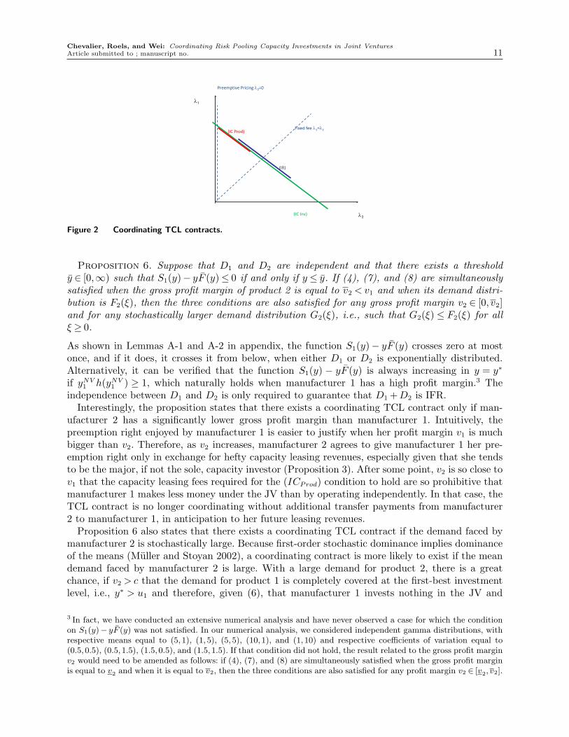
Figure 2 graphically displays the coordinating conditions derived in Propositions 2, 4 and 5.Given that the fixed-price TCL contract violates (ICProd) and the preemptive-pricing TCL contractviolates (IR), one may wonder if there exists any fully coordinating contract, i.e., any contractthat simultaneously satisfies (ICInv), (ICProd), and (IR). The next proposition characterizes theproperties of the demand and profitability of product 2, relative to the properties of product 1,such that there exists a fully coordinating contract.


λ1

λ2

(IR)

(IC Prod)

(IC Inv)

Fixed fee λ1=λ2

Preemptive Pricing λ2=0

Figure 2 Coordinating TCL contracts.

Proposition 6. Suppose that D1 and D2 are independent and that there exists a thresholdy ∈ [0,∞) such that S1(y)− yF (y)≤ 0 if and only if y ≤ y. If (4), (7), and (8) are simultaneouslysatisfied when the gross profit margin of product 2 is equal to v2 < v1 and when its demand distri-bution is F2(ξ), then the three conditions are also satisfied for any gross profit margin v2 ∈ [0, v2]and for any stochastically larger demand distribution G2(ξ), i.e., such that G2(ξ) ≤ F2(ξ) for allξ ≥ 0.

As shown in Lemmas A-1 and A-2 in appendix, the function S1(y)− yF (y) crosses zero at mostonce, and if it does, it crosses it from below, when either D1 or D2 is exponentially distributed.Alternatively, it can be verified that the function S1(y) − yF (y) is always increasing in y = y∗

if yNV1 h(yNV1 ) ≥ 1, which naturally holds when manufacturer 1 has a high profit margin.3 Theindependence between D1 and D2 is only required to guarantee that D1 +D2 is IFR.

Interestingly, the proposition states that there exists a coordinating TCL contract only if man-ufacturer 2 has a significantly lower gross profit margin than manufacturer 1. Intuitively, thepreemption right enjoyed by manufacturer 1 is easier to justify when her profit margin v1 is muchbigger than v2. Therefore, as v2 increases, manufacturer 2 agrees to give manufacturer 1 her pre-emption right only in exchange for hefty capacity leasing revenues, especially given that she tendsto be the major, if not the sole, capacity investor (Proposition 3). After some point, v2 is so close tov1 that the capacity leasing fees required for the (ICProd) condition to hold are so prohibitive thatmanufacturer 1 makes less money under the JV than by operating independently. In that case, theTCL contract is no longer coordinating without additional transfer payments from manufacturer2 to manufacturer 1, in anticipation to her future leasing revenues.

Proposition 6 also states that there exists a coordinating TCL contract if the demand faced bymanufacturer 2 is stochastically large. Because first-order stochastic dominance implies dominanceof the means (Muller and Stoyan 2002), a coordinating contract is more likely to exist if the meandemand faced by manufacturer 2 is large. With a large demand for product 2, there is a greatchance, if v2 > c that the demand for product 1 is completely covered at the first-best investmentlevel, i.e., y∗ > u1 and therefore, given (6), that manufacturer 1 invests nothing in the JV and

3 In fact, we have conducted an extensive numerical analysis and have never observed a case for which the conditionon S1(y)− yF (y) was not satisfied. In our numerical analysis, we considered independent gamma distributions, withrespective means equal to (5,1), (1,5), (5,5), (10,1), and (1,10) and respective coefficients of variation equal to(0.5,0.5), (0.5,1.5), (1.5,0.5), and (1.5,1.5). If that condition did not hold, the result related to the gross profit marginv2 would need to be amended as follows: if (4), (7), and (8) are simultaneously satisfied when the gross profit marginis equal to v2 and when it is equal to v2, then the three conditions are also satisfied for any profit margin v2 ∈ [v2, v2].


outsources her entire production to manufacturer 2. Despite manufacturer 1’s lack of investment,manufacturer 2 has sufficiently high profit prospects (in terms of sales of her own product andcapacity leasing revenues) to invest alone in the facility, and there exists a coordinating TCLcontract.

To summarize, TCL contracts are fully coordinating when the JV consists of two asymmetricpartners, namely one high-margin niche-market player (manufacturer 1) and one low-margin mass-market player (manufacturer 2). In case there exists no fully coordinating contract (and lump-sumtransfer payments are not feasible) or if imbalanced capacity investments are difficult to justify,adopting a TCL contract may not be appropriate because it could then give rise to opportunisticbehavior. In §5, we propose a variant of the capacity-leasing contract that resolves these issueswhen only two partners share one common resource.

4.3. Stability of the Negotiation Process of Coordinating ContractsWe next establish the convergence of a negotiation process to the coordinating equilibrium y∗.Instead of introducing a principal-agent framework, in which the JV would play the artificial roleof a principal dictating her terms to the founding partners, we will assume that the partner firmsagree on a process to set the capacity leasing fees. Specifically, we assume that, for any equilibriumoutcome y, the partners agree to operate the JV on a non-profit basis, i.e., that the clearingcondition λ1S1(y) + λ2S2(y) = cy holds, in addition to agreeing on the pricing scheme (e.g., fixedprice, margin sharing, preemptive pricing) of the type λ2 = γλ1, for some 0≤ γ ≤ 1. Under thesetwo conditions, we show that the partners’ negotiation process converges to the optimal contractparameter λ1 = cy∗/(S1(y∗) + γS2(y∗)) and the first-best investment level y∗.

The negotiation process works as follows. Let (λn1 , λn2 ) be the leasing fees at the beginning ofthe nth iteration, with λn2 = γλn1 , and let Πn

i (yi;y−i) be manufacturer i’s corresponding profit,i.e., Πn

i (yi;y−i) = (vi − λni )Si(y) − cyi + yiy

(λn1S1(y) +λn2S2(y)). Given these capacity-leasing fees(λn1 , γλn1 ), the parties revise their investment levels and converge to a new equilibrium (yn1 , yn2 ),which is unique under the conditions of Proposition 1 and can therefore be attained through asequential tatonnement process. Once the parties have reached an equilibrium (yn1 , yn2 ) yielding atotal investment yn = yn1 +yn2 , they update the capacity leasing fees so that the clearing condition issatisfied, i.e., they set λn+1

1 = cyn/(S1(yn)+γS2(yn)) and λn+12 = γλn+1

1 , and start the next iterationof the negotiation process. The process is repeated until convergence of the capacity leasing fees.

The next proposition shows that the capacity leasing fees will converge through this negotiationprocess to the optimal fees and the total equilibrium investment will converge to the first-bestcapacity investment level.

Proposition 7. In an iterative process where, at each iteration n, (yn1 , yn2 ) jointly solve

dΠn−1i (yni , yn−i)dyi

= 0, i= 1,2

and

λn1 = cyn

S1(yn) + γS2(yn), and λn2 = γλn1

then, for any starting point λ01, yn1 + yn2 → y∗ and λn1 → λ∗1

.= cy∗/(S1(y∗) + γS2(y∗)).

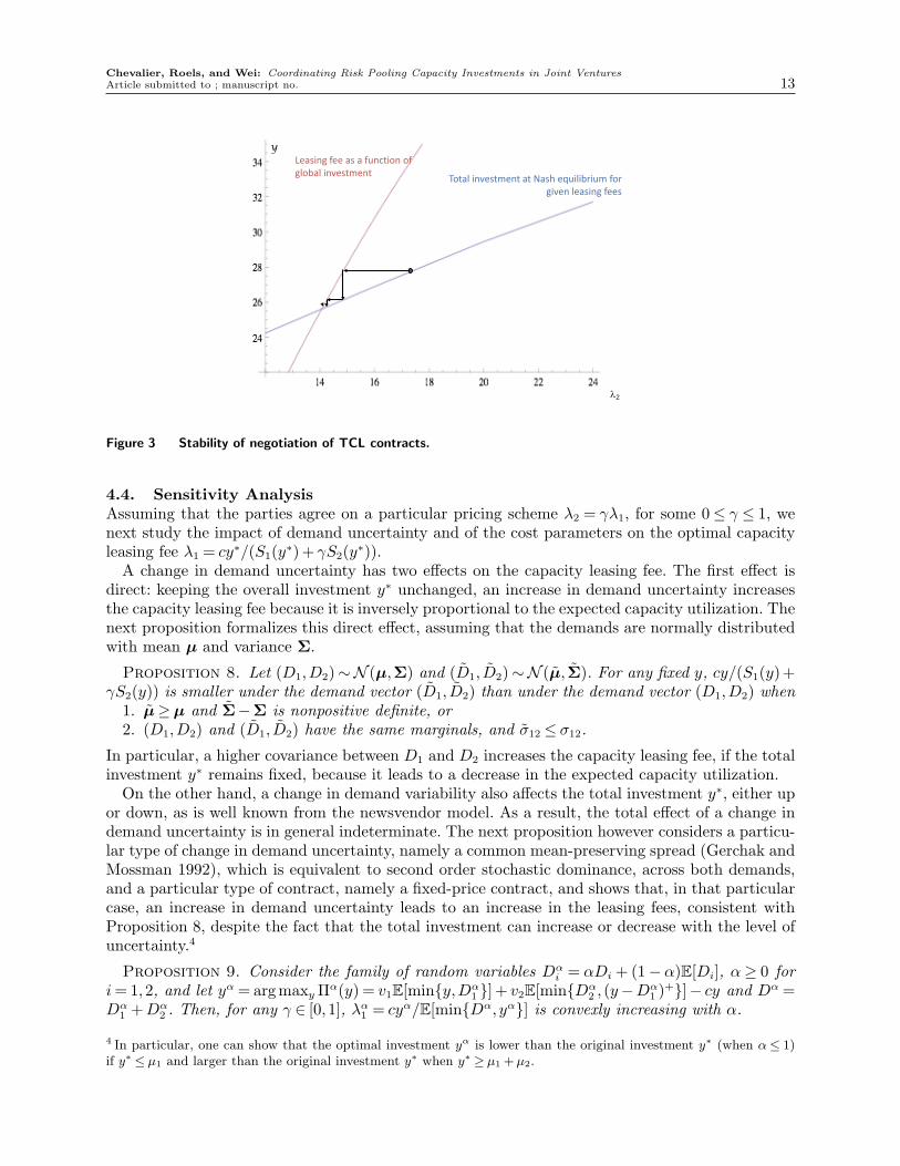
Figure 3 illustrates the negotiation process, assuming a margin-sharing (?) contract. Startingfrom a fee XXX, the partners converge, through a sequential tatonnement process, to the equi-librium. Upon reaching that equilibrium, the partners revise their leasing fees so as to satisfy theclearing condition (4). For these new leasing fees, the players then revise their offers and convergeto a new equilibrium. Continuing this process until convergence, we observe that the partnersconverge to the first-best equilibrium.


y

λ2

Total investment at Nash equilibrium for given leasing fees

Leasing fee as a function ofglobal investment

Figure 3 Stability of negotiation of TCL contracts.

4.4. Sensitivity AnalysisAssuming that the parties agree on a particular pricing scheme λ2 = γλ1, for some 0≤ γ ≤ 1, wenext study the impact of demand uncertainty and of the cost parameters on the optimal capacityleasing fee λ1 = cy∗/(S1(y∗) + γS2(y∗)).

A change in demand uncertainty has two effects on the capacity leasing fee. The first effect isdirect: keeping the overall investment y∗ unchanged, an increase in demand uncertainty increasesthe capacity leasing fee because it is inversely proportional to the expected capacity utilization. Thenext proposition formalizes this direct effect, assuming that the demands are normally distributedwith mean µ and variance Σ.

Proposition 8. Let (D1,D2)∼N (µ,Σ) and (D1, D2)∼N (µ, Σ). For any fixed y, cy/(S1(y) +γS2(y)) is smaller under the demand vector (D1, D2) than under the demand vector (D1,D2) when

1. µ≥µ and Σ−Σ is nonpositive definite, or2. (D1,D2) and (D1, D2) have the same marginals, and σ12 ≤ σ12.

In particular, a higher covariance between D1 and D2 increases the capacity leasing fee, if the totalinvestment y∗ remains fixed, because it leads to a decrease in the expected capacity utilization.

On the other hand, a change in demand variability also affects the total investment y∗, either upor down, as is well known from the newsvendor model. As a result, the total effect of a change indemand uncertainty is in general indeterminate. The next proposition however considers a particu-lar type of change in demand uncertainty, namely a common mean-preserving spread (Gerchak andMossman 1992), which is equivalent to second order stochastic dominance, across both demands,and a particular type of contract, namely a fixed-price contract, and shows that, in that particularcase, an increase in demand uncertainty leads to an increase in the leasing fees, consistent withProposition 8, despite the fact that the total investment can increase or decrease with the level ofuncertainty.4

Proposition 9. Consider the family of random variables Dαi = αDi + (1− α)E[Di], α≥ 0 for

i= 1,2, and let yα = arg maxy Πα(y) = v1E[min{y,Dα1 }] + v2E[min{Dα

2 , (y−Dα1 )+}]− cy and Dα =

Dα1 +Dα

2 . Then, for any γ ∈ [0,1], λα1 = cyα/E[min{Dα, yα}] is convexly increasing with α.

4 In particular, one can show that the optimal investment yα is lower than the original investment y∗ (when α≤ 1)if y∗ ≤ µ1 and larger than the original investment y∗ when y∗ ≥ µ1 +µ2.


We finally characterize the sensitivity of the optimal capacity-leasing fee λ1 = cy∗/(S1(y∗) +γS2(y∗)) to changes in the gross profit margins vi, i = 1,2 and capacity unit cost c. The impactof a change in the gross profit margins on the capacity leasing fees is clear: an increase in thegross profit margin of any product naturally leads to an increase in the total investment y∗ andtherefore to an increase in the capacity leasing fee. The increase in the capacity leasing fees seemshowever milder for manufacturer 1 than for manufacturer 2; in particular, one can show that, underthe margin-sharing contract, the JV’s share of manufacturer 1’s profit margin, λ1/v1, is alwaysdecreasing in v1, whereas λ2/v2 can be increasing in v2.

By contrast, an increase in the unit capacity cost generally leads to non-monotonic behavior, dueto the occurrence of two opposite effects. On the one hand, if the utilization remained unchanged,an increase in the unit capacity cost would translate into a proportional increase in the capacity-leasing fee. On the other hand, the cost increase also affects the expected capacity utilization(S1(y∗) + γS2(y∗))/y∗, by reducing the overall investment y∗, which then tends to reduce thecapacity-leasing fee. The first effect however dominates if there is not a large gap between theleasing fees λ1 and λ2.5

Proposition 10. 1. λ1 = cy∗/(S(y∗) + γS2(y∗)) and λ2 = γλ1 are increasing in v1 and v2.2. If D1 and D2 are independent, there exists a γ ∈ [0,1] such that λ1 = cy∗/(S1(y∗) + γS2(y∗))

and λ2 = γλ1 are increasing in c for all γ ≥ γ. In particular, when γ = 1, λ1 and λ2 are increasingin c.

To summarize, the sensitivity of the leasing fees really depends on the contract type. An increasein demand variability generally leads to an increase in the leasing fees, except when λ1� λ2, anincrease in the unit capacity cost generally leads to an increase in the leasing fees, except whenλ1� λ2, and an increase in profit margins always leads to an increase in the leasing fees.

5. Partial Capacity Leasing ContractsIn the previous section, we showed that TCL contracts, despite their obvious merits of leading to astable negotiation process and being easily extendable to multi-partner JVs, are fully coordinatingonly with asymmetric partners. Moreover, the overall investment is in general imbalanced, withthe most profitable manufacturer investing only marginally or nothing in the joint facility. ManyJVs however involve similar partners (e.g., Sevel Nord, Inotera) and may therefore find it difficultto justify a strict preemption right of the most profitable manufacturer on the pooled capacitywithout creating some resentment from the least profitable manufacturer.

In this section, we study a variant of the capacity leasing contract, namely the PCL contract,and show that there always exists a coordinating contract, with no restriction on the gross profitmargins and demands of the partner firms. Moreover, the capacity investments are more balanced,as the most profitable manufacturer invests generally more than under the TCL contract. Thiscontract however seems to be more complicated to negotiate than the TCL contract and does notseem to be as easily implementable in multi-partner JVs.

Under the PCL contract, the joint capacity is directly managed by the individual partner firms,and no longer by the JV. As a result, leases occur only when a partner needs extra capacity, inexcess to her own capacity, to fulfill her demand. The PCL contract works as follows:• In the investment stage, each player i invests yi in the flexible resource at a cost cyi;

5 In general however, when the gap between λ1 and λ2 is important, the fees may not be monotonically increasingin the capacity unit cost. In particular, when the unit cost c increases from slightly below v2 to slightly above v2,there may be a discontinuous drop in the optimal capacity level y∗, especially if E[D2] is large, given that product2 suddenly becomes unprofitable. This large drop in y∗ would then affect so much the utilization that the capacityleasing fees may also drop discontinuously.


• In the production stage, the quantities that maximize the joint surplus are produced. Eachplayer i collects the gross profit associated with its own sales vixi(y,D1,D2) and pays her partner aleasing fee λi for each unit of extra capacity she needs from her partner λimax{0, xi(y,D1,D2)−yi}.

Accordingly, manufacturer i’s expected profit under a PCL contract is equal to:

ΠPCLi (yi;y−i) = viSi(y)− cyi−λiE [xi(y,D1,D2)− yi]+ +λ−iE [x−i(y,D1,D2)− y−i]+ , (9)

in which x1(y,D1,D2) = min{y,D1} and x2(y,D1,D2) = min{y,D1 +D2}−x1(y,D1,D2).The PCL contract is in effect similar to the contracts adopted by Sevel-Nord and Inotera, accord-

ing to which each partner has access to 50% of the total capacity, consistent with their 50% shareof the total investment, and capacity transfers occur only in case of imbalance. It extends thestate-dependent transfer price contracts (Van Mieghem 1999) to the case where capacity transferscan occur in either direction and the transshipment price contracts (Rudi et al. 2001) to the casewhere local demands need not be satisfied first.

In contrast to TCL contracts, there is no need to use the JV as a financial intermediary and thetransfer payments can be made directly between partners. With two manufacturers, the manage-ment of this contract can therefore be more decentralized. With more manufacturers, however, itis necessary to either create a market place where capacities can be auctioned off or to appointa central authority that would unilaterally decide how to allocate the pooled capacity, similar tothe dual allocation rule proposed by Anupindi et al. (2001), potentially requiring full informationdisclosure from the JV partners (Granot and Sosic 2003). Hence, in contrast to TCL contracts,PCL contracts do not seem to be easily implementable in more complex environments.

Similar to Proposition 1, we establish the existence and the uniqueness of a Nash equilibrium inthe investment game under the PCL contract.

Proposition 11. Under a PCL contract there exists a pure-strategy Nash equilibrium in thecapacity investment game with v1 ≥ λ1 ≥ v2 ≥ λ2 ≥ 0 and λ1 ≥ c. Moreover, every such Nash equi-librium (yPCL1 , yPCL2 ) solves

dΠ1(y1;y2)

dy1= v1S

′1(y)− c+λ1P[y≥D1 ≥ y1] +λ2P[y1 ≥D1,D1 +D2 ≥ y] = 0

dΠ2(y2;y1)

dy2= v2S

′2(y)− c+λ1P[y≤D1] +λ2P[y2 ≤D2,D1 +D2 ≤ y] = 0.

(10)

If in addition, λi < vi for i= 1,2, λ1 >λ2 > 0, this Nash equilibrium is unique.

As a consequence, if λi < vi for i= 1,2 and λ1 >λ2 > 0, the game is dominance solvable, implyingCournot stability (Vives 2001).

We next investigate whether the PCL contract can coordinate the investment and productiondecisions, while ensuring participation of the partners without additional lump-sum transfer pay-ments.

Proposition 12. If there exists a Nash equilibrium (yPCL1 , yPCL2 ) in the capacity investmentgame under the PCL contract (λ1, λ2),

(ICInv) yPCL1 + yPCL2 = y∗ if and only if

λ1P[D1 ≥ yPCL1 ] +λ2P[D1 ≤ yPCL1 ,D2 ≥ yPCL2 ] = c. (11)

(ICProd) Both parties agree to allocate the pooled capacity in priority to product 1 over product2, for any demand realization, if and only if

v1 ≥ λ1 ≥ v2 ≥ λ2 ≥ 0. (12)

(IR) Both parties agree to participate to the JV without having recourse to lump-sum paymentsif (12) holds.


λ1

λ2

(IR)

(IC Prod)

(IC Inv)

Fixed fee λ1=λ2


S1’(y*)>0

λ1

λ2

(IR)

(IC Prod)

(IC Inv)

Fixed fee λ1=λ2


S1’(y*)=0

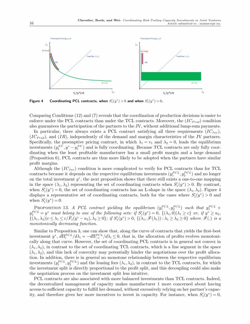
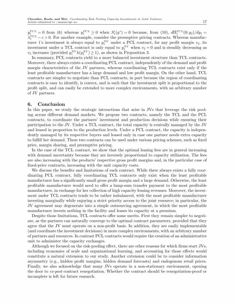
Figure 4 Coordinating PCL contracts, when S′1(y∗)> 0 and when S′1(y∗) = 0.

Comparing Conditions (12) and (7) reveals that the coordination of production decisions is easier toenforce under the PCL contracts than under the TCL contracts. Moreover, the (ICProd) conditionalso guarantees the participation of the partners to the JV, without additional lump-sum payments.

In particular, there always exists a PCL contract satisfying all three requirements (ICInv),(ICProd), and (IR), independently of the demand and margin characteristics of the JV partners.Specifically, the preemptive pricing contract, in which λ1 = v1 and λ2 = 0, leads the equilibriuminvestments (yNV1 , y∗− yNV1 ) and is fully coordinating. Because TCL contracts are only fully coor-dinating when the least profitable manufacturer has a small profit margin and a large demand(Proposition 6), PCL contracts are thus more likely to be adopted when the partners have similarprofit margins.

Although the (ICInv) condition is more complicated to verify for PCL contracts than for TCLcontracts because it depends on the respective equilibrium investments (yPCL1 , yPCL2 ) and no longeron the total investment y∗, the next proposition shows that there still exists a one-to-one mappingin the space (λ1, λ2) representing the set of coordinating contracts when S′1(y∗)> 0. By contrast,when S′1(y∗) = 0, the set of coordinating contracts has an L-shape in the space (λ1, λ2). Figure 4displays a representative set of coordinating contracts, both for the cases where S′1(y∗) > 0 andwhen S′1(y∗) = 0.

Proposition 13. A PCL contract yielding the equilibrium (yPCL1 , yPCL2 ) such that yPCL1 +yPCL2 = y∗ must belong to one of the following sets: if S′1(y∗) = 0, {(λ1,0)|λ1 ≥ c} or, if y∗ ≥ u2,{(λ1, λ2)|c≤ λ1 ≤ c/F1(y∗− u2), λ2 ≥ 0}; if S′1(y∗)> 0, {(λ1,F (λ1)) : λ1 ≥ λ2 ≥ 0} where F (.) is amonotonically decreasing function.

Similar to Proposition 3, one can show that, along the curve of contracts that yields the first-bestinvestment y∗, dΠPCL

i /dλi =−dΠPCL−i /dλi ≤ 0, that is, the allocation of profits evolves monotoni-

cally along that curve. However, the set of coordinating PCL contracts is in general not convex in(λ1, λ2), in contrast to the set of coordinating TCL contracts, which is a line segment in the space(λ1, λ2), and this lack of convexity may potentially hinder the negotiations over the profit alloca-tion. In addition, there is in general no monotone relationship between the respective equilibriuminvestments (yPCL1 , yPCL2 ) and the leasing fees (λ1, λ2), in contrast to the TCL contracts, for whichthe investment split is directly proportional to the profit split, and this decoupling could also makethe negotiation process on the investment split less intuitive.

PCL contracts are also associated with more balanced investments than TCL contracts. Indeed,the decentralized management of capacity makes manufacturer 1 more concerned about havingaccess to sufficient capacity to fulfill her demand, without excessively relying on her partner’s capac-ity, and therefore gives her more incentives to invest in capacity. For instance, when S′1(y∗) = 0,


yTCL1 = 0 from (6) whereas yPCL1 ≥ 0 when S′1(y∗) = 0 because, from (10), dΠPCL1 (0;y2)/dy1 =

λPCL1 − c > 0. For another example, consider the preemptive pricing contracts. Whereas manufac-turer 1’s investment is always equal to yNV1 under a PCL contract, for any profit margin v2, itsinvestment under a TCL contract is only equal to yNV1 when v2 = 0 and is steadily decreasing asv2 increases (provided yNV1 h(yNV1 )≥ 1), as shown in Proposition 3.

In summary, PCL contracts yield to a more balanced investment structure than TCL contracts.Moreover, there always exists a coordinating PCL contract, independently of the demand and profitmargin characteristics of the JV partners, whereas coordinating TCL contracts exist only if theleast profitable manufacturer has a large demand and low profit margin. On the other hand, TCLcontracts are simpler to negotiate than PCL contracts, in part because the region of coordinatingcontracts is easy to identify, is convex, and is such that the investment split is proportional to theprofit split, and can easily be extended to more complex environments, with an arbitrary numberof JV partners.

6. ConclusionIn this paper, we study the strategic interactions that arise in JVs that leverage the risk pool-ing across different demand markets. We propose two contracts, namely the TCL and the PCLcontracts, to coordinate the partners’ investment and production decisions while ensuring theirparticipation to the JV. Under a TCL contract, the total capacity is centrally managed by the JVand leased in proportion to the production levels. Under a PCL contract, the capacity is indepen-dently managed by its respective buyers and leased only in case one partner needs extra capacityto fulfill her demand. These two contracts can be used under various pricing schemes, such as fixedprice, margin sharing, and preemptive pricing.

In the case of the TCL contract, we show that the optimal leasing fees are in general increasingwith demand uncertainty because they are inversely proportional to capacity utilization. The feesare also increasing with the products’ respective gross profit margins and, in the particular case offixed-price contracts, increasing with the unit capacity costs.

We discuss the benefits and limitations of each contract. While there always exists a fully coor-dinating PCL contract, fully coordinating TCL contracts only exist when the least profitablemanufacturer has a significantly small gross profit margin and a large demand. Otherwise, the leastprofitable manufacturer would need to offer a lump-sum transfer payment to the most profitablemanufacturer, in exchange for her collection of high capacity leasing revenues. Moreover, the invest-ment under TCL contracts tends to be rather imbalanced, with the most profitable manufacturerinvesting marginally while enjoying a strict priority access to the joint resource; in particular, theJV agreement may degenerate into a simple outsourcing agreement, in which the most profitablemanufacturer invests nothing in the facility and leases its capacity at a premium.

Despite those limitations, TCL contracts offer some merits. First they remain simpler to negoti-ate, as the partners can naturally converge to the optimal contract parameters, provided that theyagree that the JV must operate on a non-profit basis. In addition, they are easily implementable(and coordinate the investment decisions) in more complex environments, with an arbitrary numberof partners and resources. In contrast PCL contracts would require the creation of an administrativeunit to administer the capacity exchanges.

Although we focused on the risk-pooling effect, there are other reasons for which firms start JVs,including economies of scale and organizational learning, and accounting for those effects wouldconstitute a natural extension to our study. Another extension could be to consider informationasymmetry (e.g., hidden profit margins, hidden demand forecasts) and endogenous retail prices.Finally, we also acknowledge that many JVs operate in a non-stationary environment, openingthe door to ex-post contract renegotiation. Whether the contract should be renegotiation-proof orincomplete is left for future research.


ReferencesAnupindi, R., Y. Bassok, E. Zemel. 2001. A general framework for the study of decentralized distribution

systems. Manufacturing & Service Operations Management 3(4) 349–368.Bagnoli, M., T. Bergstrom. 2005. Log-concave probability and its applications. Economic Theory 26(2)

445–469.Bamford, J., D. Ernst, D. G. Fubini. 2004. Launching a world-class joint venture. Harvard Business Review

February.Barlow, R. E., F. Proschan. 1965. Mathematical Theory of Reliability . SIAM Classics in Applied Mathemat-

ics, Philadelphia, PA.Bassamboo, A., R. S. Randhawa, J. A. Van Mieghem. 2010. Optimal flexibility configurations in newsvendor

networks: Going beyond chaining and pairing. Management Science 56(8) 1285–1303.Benett, J. 2008. VW to offer new minivan with a tuition incentive. Wall Street Journal URL http:

//online.wsj.com/article/SB121936705572662235.html. August 22, 2008.Bernstein, F., G. A. DeCroix, Y. Wang. 2007. Incentives and commonality in a decentralized multiproduct

assembly system. Operations Research 55(4) 630646.Bidault, F., M. Schweinsberg. 1996. Fiat and Peugeot SevelNord Venture (a). IMD-3-0644.Borys, B., D. B. Jemison. 1989. Hybrid arrangements as strategic alliances: Theoretical issues in organiza-

tional combinations. Academy of Management 14(2) 234–249.Cachon, G. P. 2003. Supply chain coordination with contracts. S. Graves, T. de Kok, eds., Handbook in

Oper. Res. and Management Sci.: Supply Chain Management , chap. 6. Elsevier, North-Holland.Cachon, G. P., M. A. Lariviere. 2001. Contracting to assure supply: How to share demand forecasts in a

supply chain. Management Sci. 47(5) 629–646.Deo, S., C. J. Corbett. 2009. Cournot competition under yield uncertainty: The case of the U.S. influenza

vaccine market. Manufacturing and Service Operations Management 11(4) 563–576.Dong, L., N. Rudi. 2004. Who benefits from transshipment? exogenous vs. endogenous wholesale prices.

Management Science 50(5) 645–657.Fudenber, D., J. Tirole. 1991. Game Theory . The MIT Press, Cambridge, MA.Gerchak, Y., D. Mossman. 1992. On the effects of demand randomness on inventories and costs. Operations

Research 40(4) 804–807.Granot, D., G. Sosic. 2003. A three-stage model for a decentralized distribution system of retailers. Operations

Research 51(5) 771–784.Graves, S. C., B. T. Tomlin. 2003. Process flexibility in supply chains. Management Science 49(7) 907–919.Grossman, S. J., O. D. Hart. 1986. The costs and benefits of ownership: A theory of vertical and lateral

integration. Journal of Political Economy 94(4) 691–719.Harrigan, K. R. 1988. Joint ventures and competitive strategy. Strategic Management Journal 9(2) 141–158.Harrison, J. M., J. A. Van Mieghem. 1999. Multi-resource investment strategies: Operational hedging under

demand uncertainty. European Journal of Operational Research 113(1) 17–29.Hartman, B. C., M. Dror, M. Shaked. 2000. Cores of inventory centralization games. Games and Economic

Behavior 31(1) 26–49.Hennart, J.-F. 1988. A transaction costs theory of equity joint ventures. Strategic Management Journal 9(4)

361–374.Hu, X., I. Duenyas, R. Kapuscinski. 2007. Existence of coordinating transshipment prices in a two-location

inventory model. Management Science 53(8) 1289–1302.Huang, X., G. Sosic. 2010. Transshipment of inventories: Dual allocations vs. transshipment prices. Manu-

facturing & Service Operations Management Forthcoming.Inotera. 2009. Global depositary shares offering circular.Jolly, D. 1997. Co-operation in a niche market: The case of Fiat and PSA in multi purpose vehicles. European

Management Journal 15(1) 35–44.


Jordan, W. C., S. C. Graves. 1995. Principles on the benefits of manufacturing process flexibility. ManagementScience 41(4) 577–594.

Karp, A. 2006. Maintaining a mammoth. URL http://atwonline.com/operations-maintenance/article/maintaining-mammoth-0309. Air Transport World.

Kogut, B. 1988. Joint ventures: Theoretical and empirical perspectives. Strategic Management Journal 9(4)319–332.

Krishnan, H., T. McCorrmick, J. Shao. 2010. Incentives for transshipment in a supply chain with decentral-ized retailers. Working Paper, University of British Columbia.

Lariviere, M. A., E. L. Porteus. 2001. Selling to the newsvendor: An analysis of price-only contracts. Man-ufacturing Service Oper. Management 3(4) 293–305.

Lippman, S. A., K. F. McCardle. 1997. The competitive newsboy. Operations Research 45(1) 54–65.

Mcdonald, Gareth. 2008. U.S. government pays Sanofi Pasteur $192m for bulkflu antigen. URL http://www.in-pharmatechnologist.com/Industry-Drivers/US-govt-pays-Sanofi-Pasteur-192m-for-bulk-flu-antigen.

Muller, A., M. Scarsini, M. Shaked. 2002. The newsvendor game has a nonempty core. Games and EconomicBehavior 38(1) 118–126.

Muller, A., D. Stoyan. 2002. Comparison Methods for Stochastic Models and Risks. John Wiley & Sons,Chichester, West Sussex, PO19 IUD, England.

Netessine, S., N. Rudi. 2003. Centralized and competitive inventory models with demand substitution. Oper.Res. 51(2) 329–335.

News, Flight Daily. 2007. Spairliners spools up. URL http://www.flightglobal.com/articles/2007/06/20/214885/spairliners-spools-up.html.

Perakis, G., G. Roels. 2007. The Price of Anarchy in supply chains: Quantifying the efficiency of price-onlycontracts. Management Sci. 53(8) 1249–1268.

Porteus, E. L. 1990. Stochastic inventory theory. D. Heyman, M. Sobel, eds., Handbook in OperationsResearch and Management Science, vol. 2. Elsevier North-Holland, Amsterdam, 605–653.

Roos, R. 2007. Flu vaccine makers get HHS funds to prepapre for pandemics. URL http://id_center.apic.org/cidrap/content/influenza/panflu/news/jun2007vaccine.html.

Rudi, N., S. Kapur, D. F. Pyke. 2001. A two-location inventory model with transshipment and local decisionmaking. Management Science 47(12) 1668–1680.

Suakkaphong, N., M. Dror. 2009. Competition and cooperation in decentralized distribution. Working Paper,The University of Arizona.

Topkis, D. M. 1998. Supermodularity and Complementarity . Princeton University Press, Princeton, NJ.

Van Mieghem, J. A. 1998. Investment strategies for flexible resources. Management Science 44(8) 1071–1078.

Van Mieghem, J. A. 1999. Coordinating investment, production and subcontracting. Management Science45(7) 954–971.

Van Mieghem, J. A. 2003. Capacity management, investment, and hedging: Review and recent developments.Manufacturing & Service Operations Management 5(4) 269302.

Van Mieghem, J. A., N. Rudi. 2002. Newsvendor networks: Inventory management and capacity investmentwith discretionary activities. Manufacturing & Service Operations Management 4(4) 313–335.

Vives, X. 2001. Oligopoly Pricing. Old Ideas and New Tools. The MIT Press, Cambridge, MA.

e-companion to Chevalier, Roels, and Wei: Coordinating Risk Pooling Capacity Investments in Joint Ventures ec1

This page is intentionally blank. Proper e-companion titlepage, with INFORMS branding and exact metadata of themain paper, will be produced by the INFORMS office whenthe issue is being assembled.

ec2 e-companion to Chevalier, Roels, and Wei: Coordinating Risk Pooling Capacity Investments in Joint Ventures

Proofs of StatementsProof of Proposition 1. By the Weierstrass theorem, for any y−i, ΠTCL

i (yi;y−i) attains a max-imum on [−y−i,∞) because it is continuous and because limyi→∞ΠTCL

i (yi;y−i) =−∞. Summingup the necessary optimality conditions (3), we obtain that a Nash equilibrium (yTCL1 , yTCL2 ), if itexists, must solve v1S

′1(y) + v2S

′2(y)− c+ (λ1S1(y) + λ2S2(y))/y− c= 0 and y = yTCL1 + yTCL2 . For

any y < y∗, v1S′1(y)+v2S

′2(y)−c > 0 by (1) and (λ1S1(y)+λ2S2(y))/y−c≥ 0 because y∗ ≤ y; hence

yTCL1 +yTCL2 ≥ y∗. On the other hand, for any y > y, v1S′1(y)+v2S

′2(y)−c < 0 by (1), because y∗ ≤ y,

and (λ1S1(y) + λ2S2(y))/y − c≤ 0; hence, yTCL1 + yTCL2 ≤ y. Therefore, for any y−i, ΠTCLi (yi;y−i)

attains its maximum on [y∗− y−i, y− y−i].Moreover, if there exists an equilibrium with yTCLi < 0, there also exists an equilibrium with

yTCLi ≥ 0 because

dΠTCLi (0;y−i)dyi

= (vi−λi)S′i(y)− c+1y

(λ1S1(y) +λ2S2(y))≥ (vi−λi)S′i(y)≥ 0,

in which the first inequality used the fact that (λ1S1(y) +λ2S2(y))/y−c≥ (λ1S1(y) +λ2S2(y))/y−c= 0 for any y ≤ y. Therefore, without loss of generality, one can restrict the strategy spaces tothe compact sets [(y∗− y−i)+, (y− y−i)+].

When y2/y≤ (v2−λ2)/(λ1−λ2), the derivative of manufacturer 2’s profit function is nonnegative:

dΠTCL2 (y2;y1)dy2

= (v2−λ2)S′2(y)− c+1y

(λ1S1(y) +λ2S2(y))

+y2

y

(λ1S

′1(y) +λ2S

′2(y)− 1

y(λ1S1(y) +λ2S2(y))

)≥ (v2−λ2)S′2(y)− c+

1y

(λ1S1(y) +λ2S2(y))

+v2−λ2

λ1−λ2

(λ1S

′1(y) +λ2S

′2(y)− 1

y(λ1S1(y) +λ2S2(y))

)=v2−λ2

λ1−λ2

(λ1S

′(y)− 1y

(λ1S1(y) +λ2S2(y)))− c+

1y

(λ1S1(y) +λ2S2(y))

≥(

1− v2−λ2

λ1−λ2

)(1y

(λ1S1(y) +λ2S2(y))− c)≥ 0,

in which the first inequality used the fact that the function λ1S1(y) + λ2S2(y) = (λ1 −λ2)S1(y) + λ2S(y) is concave increasing. The second inequality used the fact that S′(y)≥ S′(y)≥c/λ1 for any y ≤ y, and the third inequality used the fact that (λ1S1(y) +λ2S2(y))/y − c ≥(λ1S1(y) +λ2S2(y))/y− c= 0 for any y≤ y.

On the other hand, when y2/y ≤ (v2−λ2)/(λ1−λ2) and y1 ≥ 0, the second derivative of manu-facturer 2’s profit function is nonpositive:

d2ΠTCL2 (y2;y1)dy2

2

= (v2−λ2)S′′2 (y) +y2

y(λ1S

′′1 (y) +λ2S

′′2 (y))

+2y1

y2

(λ1S

′1(y) +λ2S

′2(y)− 1

y(λ1S1(y) +λ2S2(y))

)≤ (v2−λ2)S′′2 (y) +

y2

y(λ1S

′′1 (y) +λ2S

′′2 (y))

=(v2−λ2

y1

y

)S′′(y) +

((λ1−λ2)

y2

y− (v2−λ2)

)S′′1 ≤ 0,


in which the first inequality used the fact that the function λ1S1(y) + λ2S2(y) = (λ1− λ2)S1(y) +λ2S(y) is concave increasing, and the second inequality used the condition on y2/y and on y1,together with the concavity of the functions S1(y) and S(y).

As a result, when y1 ≥ 0, ΠTCL2 (y2;y1) is quasiconcave, increasing when y2/y≤ (v2−λ2)/(λ1−λ2)

and concave when y2/y≥ (v2−λ2)/(λ1−λ2). On the other hand, manufacturer 1’s profit functionΠTCL

1 (y1;y2) is concave for all y1 ≥ 0 because (v1−λ1)S1(y), (y1/y)(λ1−λ2)S1(y), (y1/y)λ2S(y), and−cy1 are all concave in y1. Because both players’ profit function are continuous and quasiconcaveon [(y∗ − y−i)+, (y − y−i)+] and their respective strategy sets are compact, there exists a Nashequilibrium (Fudenberg and Tirole 1991, p. 34).

If moreover λ1E[D1] + λ2E[D2] ≤ 2cu, there is no equilibrium such that y > u. Suppose, forcontradiction, that y > u. Accordingly, Si(y) = E[Di] and S′i(y) = 0, for i = 1,2, and thereforedΠTCL

i (yi;y−i)/dyi =−c+ yiy2

(λ1E[D1] +λ2E[D2]) = 0 for i= 1,2. Because dΠTCLi (yi;y−i)/dyi = 0

for i= 1,2, we must then have y1 = y2 = y/2. The equilibrium conditions would then simplify todΠTCL

i (yi;y−i)/dyi = −c + 12y

(λ1E[D1] +λ2E[D2]) < −c + 12u

(λ1E[D1] +λ2E[D2]) ≤ 0, which is acontradiction.

Finally, we prove uniqueness of the equilibrium by using the Poincare-Hopf index theorem, i.e.,by showing that the Jacobian matrix associated with the equilibrium conditions (3) and evaluatedat any equilibrium point (yTCL1 , yTCL2 ) is negative definite (Vives 2001, p. 47). By assumption,f(ξ)> 0 for any ξ ∈ [l, u] and f1(ξ)> 0 for any ξ ∈ [l1, u1]. Therefore, if u1 > l, either S′′1 (y)< 0 orS′′(y)< 0 for any y ∈ [l1, u] and in particular at any equilibrium point given that yTCL ≥ y∗ ≥ l1and that yTCL ≤ u when λ1E[D1] +λ2E[D2]≤ 2cu.

Hence, for any y ∈ [l1, u], ∂2ΠTCL1 (y1;y2)

∂y21= (v1 − λ1)S′′1 (y) + (y1/y) ((λ1−λ2)S′′1 (y) +λ2S

′′(y)) +2(y2/y

2) ((λ1−λ2)S′1(y) +λ2S′(y))− 2(y2/y

3) ((λ1−λ2)S1(y) +λ2S(y))< 0 when v1 >λ1 >λ2 > 0.For any y, the determinant of the Jacobian can be written as

|J | =(λ1S

′1(y) +λ2S

′2(y)− 1

y(λ1S1(y) +λ2S2(y))

)2

+1y

(λ1S

′1(y) +λ2S

′2(y)− 1

y(λ1S1(y) +λ2S2(y))

)((v1− v2)S′′1 (y) + v2S

′′(y))

and is strictly positive when y ∈ [l1, u], and in particular at any equilibrium point, given that eitherS1(y) or S(y) is strictly concave, that v1 > v2 > 0, and that λ1 >λ2 > 0. Q.E.D.

Proof of Proposition 2. Suppose that there exists a Nash equilibrium satisfying (3) suchthat y1 + y2 = y∗. Summing up (3), we obtain: 0 = (v1 − v2)S′1(y∗) + v2S

′(y∗) − c +1y∗ ((λ1−λ2)S1(y∗) +λ1S(y∗))− c. Because (1) holds, (4) must also hold.

To see the converse, suppose that there exists a Nash equilibrium satisfying (3) such that(4) holds. Summing up the equilibrium conditions (3), we obtain: (v1 − v2)S′1(y) + v2S

′(y)− c+1y

((λ1−λ2)S1(y) +λ2S(y))− c= 0. By assumption, S′′(y)< 0 for any y ∈ [l, u] and S′′1 (y)< 0 forany y ∈ [l1, u1], and the left-hand side is strictly decreasing in y. Hence, there exists a unique y,namely y∗, such that this equality holds. The equilibrium profits are then simply obtained bysubstituting (4) into (2). Q.E.D.

Proof of Proposition 3. Applying the chain rule to (2), we get

dΠTCLi (yTCLi ;yTCL−i )

dλi=∂ΠTCL

i (yTCLi ;yTCL−i )∂λi

+∂ΠTCL

i (yTCLi ;yTCL−i )∂yi

dyTCLi

dλi+∂ΠTCL

i (yTCLi ;yTCL−i )∂y−i

dyTCL−i

dλi

=∂ΠTCL

i (yTCLi ;yTCL−i )∂λi

=−Si(yTCL)yTCL−i

yTCL=−

∂ΠTCL−i (yTCL−i ;yTCLi )

∂λi,

in which the first equality follows from the fact that ∂ΠTCLi (yTCLi ;yTCL−i )/∂yi = 0 in equilibrium and

that ∂ΠTCLi (yTCLi ;yTCL−i )/∂y−i = 0 when (4) holds. Moreover, because −Si(yTCL)yTCL−i /yTCL ≤ 0,

dΠTCLi (yTCLi ;yTCL−i )/dλi ≤ 0.


From (5) and (6), we obtain that yTCL1 /yTCL2 = (ΠTCL1 /ΠTCL

2 ) (S′1(y∗)S2(y∗)/ (S1(y∗)S′2(y∗))).Hence, yTCL1 /yTCL2 is directly proportional to ΠTCL

1 /ΠTCL2 . Therefore dyTCLi /dλi =−yTCL−i /dλi ≤ 0.

Finally, we show that, when λ2 = γλ1, yTCL1 is nonincreasing in v2. Expressing yTCL1 as(yTCL1 /y∗)y∗ and taking the derivative with respect to v2, we obtain:

dyTCL1

dv2

=d(yTCL1y∗

)dv2

y∗+yTCL1

y∗dy∗

dv2

=dyTCL1y∗

dy∗dy∗

dv2

y∗+yTCL1

y∗dy∗

dv2

.

When λ2 = γλ1, (4) yields that λ1 = cy∗/(S1(y∗) + γS2(y∗)), and therefore (6) can be expressed asfollows:

yTCL1

y∗=

(v1(S1(y∗) + γS2(y∗))− cy∗)S′1(y∗)c(S1(y∗) + γS2(y∗))− cy∗(S′1(y∗) + γS′2(y∗))

.

Accordingly,

d(yTCL1y∗

)dy∗

= S′1(y∗)−−S

′′1 (y∗)

S′1(y∗) (v1(S1(y∗) + γS2(y∗))− cy∗) + (v1(S′1(y∗) + γS′2(y∗))− c)− cyTCL1

−(S′′1 (y∗)+γS′′2 (y∗))S′1(y∗)

c(S1(y∗) + γS2(y∗))− cy∗(S′1(y∗) +S′2(y∗)).

Therefore, yTCL1 is nonincreasing in v2 if and only if d(yTCL1 /y∗)/dy∗+ yTCL1 /(y∗)2 ≤ 0, or equiv-alently, if and only if the following function

G(y∗) :=(

1y∗− −S

′′1 (y∗)

S′1(y∗)

)(v1(S1(y∗) + γS2(y∗))− cy∗) + (v1(S′1(y∗) + γS′2(y∗))− c)

−cyTCL1

− (S′′1 (y∗) + γS′′2 (y∗))S′1(y∗)

is nonpositive.Suppose that γ ≤ v2/v1. Then, v1(S′1(y∗) + γS′2(y∗)) − c ≤ 0 by (1). Moreover, the first term

in G(y∗) is nonpositive because, on the one hand, −y∗S′′1 (y∗)/S′1(y∗) = y∗h1(y∗)≥ yNV1 h1(yNV1 )≥yNV1 h(yNV1 )≥ 1 because h1(y)≥ h(y) (when D1 and D2 are independent IFR) and yNV1 h(yNV1 )≥ 1,and on the other hand, v1(S1(y∗) +γS2(y∗))− cy∗ = (v1−λ1)(S1(y∗) +γS2(y∗))≥ 0 by (4). Finally,it is trivial to check that the third term in G(y∗) is also nonpositive. Therefore in G(y∗) ≤ 0,demonstrating that yTCL1 is nonincreasing in v2 when γ ≤ v2/v1 and yNV1 h(yNV1 )≥ 1.

On the other hand, when γ ≥ v2/v1, G(y∗) is decreasing in y∗ when dyTCL1 /dy∗ = 0 because(1y∗− −S

′′1 (y∗)

S′1(y∗)

)′= − 1

(y∗)2−h′1(y∗)≤ 0,

(v1(S1(y∗) + γS2(y∗))− cy∗)′ = v1(S′1(y∗) + γS′2(y∗))− c≥ 0,(v1(S′1(y∗) + γS′2(y∗))− c)′ = v1(S′′1 (y∗) + γS′′2 (y∗)) = v1γS

′′(y∗) + v1(1− γ)S′′1 (y∗)≤ 0,(−S′′1 (y∗)− γS′′2 (y∗)

S′1(y∗)

)′=(−(1− γ)S′′1 (y∗)− γS′′(y∗)

S′1(y∗)

)′= (1− γ)h′1(y∗) + γ

F (y∗)F1(y∗)

(f ′(y∗)F (y∗)

+h1(y∗)h(y∗))

≥ (1− γ)h′1(y∗) + γF (y∗)F1(y∗)

(f ′(y∗)F (y∗)

+h2(y∗))

= (1− γ)h′1(y∗) + γF (y∗)F1(y∗)

h′(y∗)≥ 0,


in which we used the facts that h1(y)≥ h(y) and h′(y)≥ 0 (when D1 and D2 are independent andIFR, Theorems 5.1 and 5.4 in Barlow and Proschan 1965). Hence, when dyTCL1 /dy∗ = 0, the secondderivative of yTCL1 is nonpositive. That is, yTCL1 is quasiconcave in v2.

Hence, to show that yTCL1 is nonincreasing in v2, it remains to show G(y∗) ≤ 0 whenv2 = 0, or equivalently, by (1) when y∗ = yNV1 . The first term in G(y∗) is nonpositive whenyNV1 h1(yNV1 ) ≥ 1. The second term, when y∗ = yNV1 , can be bounded as follows: v1(S′1(y∗) +γS′2(y∗)) − c = γ(S′(y∗) − S′1(y∗)) ≤ γS′(y∗). Finally, by (6), yTCL2 ≤ 0 because λ2 ≥ 0 whenγ ≥ 0, and therefore yTCL1 ≥ y∗; as a result, the third term in G(y∗) can be bounded as fol-lows: −cyTCL1 (−S′′1 (y∗)− γS′′2 (y∗))/S′1(y∗) =−v1y

TCL1 (f1(y∗)(1− γ) + γf(y∗))≤−v1y

TCL1 γf(y∗)≤

−v1y∗γf(y∗) = −v1y

∗γh(y∗)S′(y∗) ≤ −v1γS′(y∗), in which we used the fact that yNV1 h(yNV1 ) ≥ 1.

Combining these last two results, we obtain that G(yNV1 )≤ 0, i.e., that yTCL1 is nonincreasing inv2, completing the proof. Q.E.D.

Proof of Proposition 4. For i = 1,2, manufacturer i’s ex-post profit is equal to (vi − λi)xi +yiy∗ (λ1x1 +λ2x2). Hence, manufacturer 1 prefers to produce product 1 if and only if v1 ≥ λ1

y2y∗ +λ2

y1y∗

and manufacturer 2 prefers to produce product 1 if and only if v2 ≤ λ1y2y∗ + λ2

y1y∗ . Combining the

two conditions, the two manufacturers agree to give priority to product 1 if and only if

v1 ≥ λ1

y2

y∗+λ2

y1

y∗≥ v2. (A-1)

Substituting the equilibrium investment levels (6) into (A-1), and using the fact that λ1S′1(y∗) +

λ2S′2(y∗)≤ c= λ1S1(y∗)/y∗+λ2S2(y∗)/y∗, we obtain that (A-1) holds if and only if

v1 (c−λ1S′1(y∗)−λ2S

′2(y∗))≥ λ1(v2−λ2)S′2(y∗) +λ2(v1−λ1)S′1(y∗)≥ v2 (c−λ1S

′1(y∗)−λ2S

′2(y∗)) .

Rearranging the terms, and using (1) and vi ≥ λi for i= 1,2, one can simplify this condition to

λ1 ≥c

S′(y∗)≥ λ2. (A-2)

From (1), we obtain that S′(y∗)≤ c/v2. Using this result together with (A-2) yields the propo-sition statement. Q.E.D.

Proof of Proposition ??. The statement follows from requiring that ΠTCLi (yTCLi , yTCL−i ) ≥

ΠNVi (yNVi ), in which ΠTCL

i (yTCLi , yTCL−i ) is expressed by (5). Q.E.D.Proof of Proposition 6. From (4), we obtain that λ1 = cy∗/S1(y∗)δ and λ2 = cy∗/S2(y∗)(1− δ),

for some δ. Condition (8) is thus satisfied if

v1S1(y∗)−ΠNV1 (yNV1 )

cy∗≥ δ≥ 1− v2S2(y∗)−ΠNV

2 (yNV2 )cy∗

. (A-3)

Note that the interval is not empty because ΠNV1 (yNV1 ) + ΠNV

2 (yNV2 ) ≤ Π(y∗). Clearly, if (8) issatisfied, then v1 ≥ λ1 because ΠNV

1 (yNV1 )≥ 0; moreover, v2 ≤ c/F (y∗) is always satisfied from (1).Hence, in order for (7) to be satisfied, we need

δ≥ S1(y∗)y∗F (y∗)

. (A-4)

and

δ≥ 1− v2S2(y∗)cy∗

. (A-5)


Conditions (A-3) and (A-5) are always compatible if (v1S1(y∗) − ΠNV1 (yNV1 ))/(cy∗) ≥ 1 −

(v2S2(y∗))/(cy∗), which always holds given that Π(y∗)≥ΠNV1 (yNV1 ). On the other hand, Conditions

(A-3) and (A-4) are compatible if

v1S1(y∗)−ΠNV1 (yNV1 )

cy∗≥ S1(y∗)y∗F (y∗)

,

that is, if

S1(y∗)(v1−

c

F (y∗)

)≥ΠNV

1 (yNV1 ). (A-6)

The left-hand side function G(y) := S1(y)(v1− c/F (y)

)is concave in y, because its sec-

ond derivative G′′(y) = −f1(y)(v1− c/F (y)

)− 2cF1(y)f(y)/(F (y))2 − c (f(y))2

/(F (y)

)3S1(y) −

cS1(y)/F (y)h′(y) is nonpositive. Therefore G(y) has convex level sets. Hence, because y∗ is increas-ing in v2 by (1), if (A-6) is satisfied for some v2 and v2, it is also satisfied for any v2 ∈ [v2, v2].Moreover, we note from (1) that y∗ is equal to F−1(c/v1) when v2 = v1 and that limy↑F−1(c/v1)G(y) =0<ΠNV

1 (yNV1 ); hence v2 < v1.We next show that if (A-6) is not satisfied when v2 = 0 then (A-6) is never satisfied, for any

v2 ≥ 0. Because G(y) is concave and y∗ is increasing in v2 by (1), we just need to show that atv2 = 0, if (A-6) is not satisfied, then G′(y∗)≤ 0. From (1), we obtain that at v2 = 0, y∗ is equal toyNV1 = F−1

1 (c/v1). Hence, (A-6) is not satisfied at v2 = 0 if and only if

S1(yNV1 )− yNV1 F (yNV1 )> 0. (A-7)

Using F1(yNV1 ) = c/v1 and (A-7), we obtain:

G′(y∗)|v2=0 =c

F (yNV1 )

(F (yNV1 )− F1(yNV1 )−S1(yNV1 )

f(yNV1 )F (yNV1 )

)≤ c

F (yNV1 )(F (yNV1 )− F1(yNV1 )− yNV1 f(yNV1 )

), (A-8)

and the inequality is tight when S1(yNV1 )− yNV1 F (yNV1 ) = 0. Because the function S1(y)− yF (y)crosses zero only once by assumption, its derivative, equal to F1(y)− F (y) + yf(y), is nonnegativewhen S1(y)− yF (y) = 0, therefore showing that the right-hand side of (A-8) is nonpositive, i.e.,that at v2 = 0, G′(y∗)≤ 0 when (A-6) is not satisfied.

We finally establish the result with respect to the demand distribution of product 2. Using (1),we rewrite (A-6) as follows:

S1(y∗)(v1−

cv2

c− (v1− v2)F1(y∗)

)≥ΠNV

1 (yNV1 ). (A-9)

The left-hand side depends on the demand distribution of product 2 only through y∗, whereas theright-hand side is independent of D2. Let D2 and D2 be two random variables representing thedemand for product 2, with respective distributions F2(ξ) and G2(ξ). Then, D2 ≥st D2 if G2(ξ)≤F2(ξ) for all ξ. Let G(ξ) = P[D1 + D2 ≤ ξ] and F (ξ) = P[D1 +D2 ≤ ξ]. By Theorem 1.2.17 in Mullerand Stoyan (2002), we obtain D1 + D2 ≥stD1 +D2, i.e., G(ξ)≥ F (ξ) for all ξ. Let y∗ and y∗ be thefirst-best investment levels when the demand distributions of product 2 are respectively D2 andD2. Because (v1− v2)F1(y∗) + v2G(y∗)≥ (v1− v2)F1(y∗) + v2F (y∗) = c= (v1− v2)F1(y∗) + v2G(y∗),we obtain that y∗ ≥ y∗ by concavity of Π(y). Because H(y) := S1(y)

(v1− cv2/(c− (v1− v2)F1(y))

)is increasing in y, we have H(y∗)≥H(y∗); hence, if (A-9) is satisfied under demand D2, it is alsosatisfied under D2 ≥stD2. Q.E.D.


Lemma A-1. Suppose D1 and D2 are independent. If D1 is exponentially distributed, there existsa threshold y ∈ [0,∞) such that S1(y)− yF (y)≤ 0 if and only if y≤ y.

Proof. In order to prove the existence of such a threshold, it is sufficient to show that thederivative of S1(y)− yF (y), equal to F1(y)− F (y) + f(y)y, is positive whenever S1(y)− yF (y) = 0and y > 0. Given that Di are IFR for i = 1,2, D1 + D2 is also IFR, i.e., h′(ξ) ≥ 0. Using theidentity F (y) = exp

[−∫ y

0h(ξ)dξ

](see Equation (2.1) in Barlow and Proschan 1965), we obtain

F (y) = exp[−∫ y

0h(ξ)dξ

]≥ exp [−yh(y)], and therefore yh(y)≥− ln

(F (y)

). Accordingly, we obtain(

F1(y)− F (y) + f(y)y) ∣∣∣S1(y)=yF (y)

≥(F1(y)− F (y)− F (y) ln

(F (y)

)) ∣∣∣S1(y)=yF (y)

= F1(y)− S1(y)y− S1(y)

yln(S1(y)y

).

When D1 follows a negative exponential distribution with parameter λ, y = − ln(ϕ)/λ andS1(y) = (1− ϕ)/λ, in which ϕ = F (y). Substituting these expressions into the right-hand side ofthe above inequality, we obtain(

F1(y)− F (y) + f(y)y) ∣∣∣S1(y)=yF (y)

≥ϕ+1−ϕln(ϕ)

+1−ϕln(ϕ)

ln(

1−ϕ− ln(ϕ)

)It can be then be verified that the right-hand side of this inequality is always positive for any0≤ϕ< 1, i.e., for any y ∈ (0,∞), completing the proof. Q.E.D.

Lemma A-2. Suppose D1 and D2 are independent. If D2 is exponentially distributed, there existsa threshold y ∈ [0,∞) such that S1(y)− yF (y)≤ 0 if and only if y≤ y.

Proof. When D1 and D2 are independent, F (y) =∫ y

0F2(y − ξ)f1(ξ)dξ + F1(y) and f(y) =∫ y

0f2(y− ξ)f1(ξ)dξ. Hence, given that D2 is IFR, we have

F1(y)− F (y) + f(y)y =∫ y

0

(yf2(y− ξ)− F2(y− ξ)

)f1(ξ)dξ

≥ (h2(0)y− 1)∫ y

0

F2(y− ξ)f1(ξ)dξ.

Let λ= h2(0). We must have that λy≥ 1 when S1(y)− yF (y) = 0 because otherwise F2(y−x) =exp [−(y−x)λ]> exp [−(y−x)/y]≥ x/y for all x≤ y, and therefore F (y) =

∫ y0F2(y− ξ)f1(ξ)dξ +

F1(y)>∫ y

0(ξ/y)f1(ξ)dξ + F1(y) = S1(y)/y, a contradiction. As a result, when D2 is exponentially

distributed, we obtain:(F1(y)− F (y) + f(y)y

) ∣∣∣S1(y)=yF (y)

≥(

(λy− 1)∫ y

0

F2(y− ξ)f1(ξ)dξ)∣∣∣

S1(y)=yF (y)≥ 0.

Hence, the function S1(y)− yF (y)≤ 0 crosses zero at most once, and if it does, it crosses it frombelow. Q.E.D.

Proof of Proposition 7. The proof is by induction. Suppose that, at the n-th iteration, yn ≤ y∗.Let Π(y) = Π1(y)+Π2(y) =R(y)−cy be the total profit function. By concavity of Π(y), Π′(yn)≥ 0.On the other hand, because (yn1 , yn2 ) defines a Nash equilibrium when (λ1, λ2) = (λn−1

1 , γλn−11 ), we

have

0 =dΠn−1

1 (yn1 , yn2 )dy1

+dΠn−1

2 (yn2 , yn1 )dy2

= Π′(yn) +λn−1

1

yn(S1(yn) + γS2(yn))− c (A-10)

and therefore λn−11 ≤ cyn/(S1(yn) + γS2(yn)) .= λn1 . Moreover, one can show from (A-10) that yn is

increasing with λn−11 using the implicit function theorem. Hence, yn+1 ≥ yn. On the other hand,


because yn ≤ y∗ by assumption, cyn/(S1(yn) + γS2(yn))≤ cy∗/(S1(y∗) + γS2(y∗)). Therefore, λn1 ≤λ∗1; hence yn+1 ≤ y∗. Because the sequence {yn} is monotone and bounded, it is convergent.

The limit point of this sequence (y∞, λ∞1 ) jointly solves Π′(y∞) + λ∞1y∞ (S1(y∞) + γS2(y∞))− c= 0

and λ∞1 = c y∞

S1(y∞)+γS2(y∞). In particular, y∞ solves Π′(y∞) = 0. Because Π(y) is strictly concave

when f12(ξ1, ξ2) is log-concave, y∞ = y∗, and therefore λ∞1 = λ∗1. Similarly, one can show that ifyn ≥ y∗, the sequence {yn, λn1} is monotone and bounded, and converges to (y∗, λ∗1). Q.E.D.

Proof of Proposition 8. 1. From Muller and Stoyan (2002), X ≥SSD Y if Eg(X)≥Eg(Y ) forall increasing concave functions g. Hence, for any given y, because min{y,D1} is concave increasingin D1 and min{y,D1 +D2} is concave increasing in D1 +D2, cy/((1− γ)S1(y) + γS(y)) is smallerunder the demand vector (D1, D2) than under (D1,D2) when D1 ≥SSD D1 and D1 + D2 ≥SSDD1 +D2. The statement then follows from Theorem 3.4.8 in Muller and Stoyan (2002).

2. From Muller and Stoyan (2002), the vector X is larger than the vector Y in the super-modular order, written X ≥sm Y, if Eg(X) ≥ Eg(Y) for all supermodular functions g. Forany given y, it can be verified using Lemma 2.6.4 and Corollary 2.6.2 in Topkis (1998) thatthe functions −E[min{y,D1} and −E[min{y,D1 +D2} are supermodular in (D1,D2). Therefore,cy/((1− γ)S1(y) + γS(y)) is smaller under the demand vector (D1, D2) than under (D1,D2) when(D1, D2)≤sm (D1,D2), which holds by Theorem 3.1.13.5 in Muller and Stoyan (2002). Q.E.D.

Proof of Proposition 9. Let y∗ = y1 be the optimal investment level when α = 1 and let λ∗1 =λ∗2 = cy∗/S(y∗) be the corresponding leasing fee under the fixed-price contract. Let also µi = E[Di].Then, by optimality of y∗ and yα when the demand random variables are (D1,D2) and (Dα

1 ,Dα2 ),

we have

0 = (v1− v2)P(D1 ≥ y∗) + v2P(D1 +D2 ≥ y∗)− c= (v1− v2)P(Dα

1 ≥ yα) + v2P(Dα1 +Dα

2 ≥ yα)− c

= (v1− v2)P(D1 ≥

yα− (1−α)µ1

α

)+ v2P

(D1 +D2 ≥

yα− (1−α)(µ1 +µ2)α

)− c

≥ (v1− v2)P(D1 ≥

yα− (1−α)(µ1 +µ2)α

)+ v2P

(D1 +D2 ≥

yα− (1−α)(µ1 +µ2)α

)− c,

if and only if α≥ 1. Therefore, by concavity of the profit function v1S1(y) + v2S2(y)− cy,

yα− (1−α)(µ1 +µ2)α

≥ y∗ (A-11)

if and only if α≥ 1 .On the other hand, we have

λα1 =cyα

E[min{Dα, yα}]= c

α yα−(1−α)(µ1+µ2)

α+ (1−α)(µ1 +µ2)

αE[min

{D, y

α−(1−α)(µ1+µ2)

α

}]+ (1−α)(µ1 +µ2)

= cαz+ (1−α)(µ1 +µ2)

αE [min{D,z}] + (1−α)(µ1 +µ2)

with z = yα−(1−α)(µ1+µ2)

α. The right-hand side is increasing with z, for any α, by concavity of S(z).

Using (A-11), we obtain

λα1 ≥ cαy∗+ (1−α)(µ1 +µ2)

αE [min{D,y∗}] + (1−α)(µ1 +µ2)

if and only if α≥ 1. The right-hand side is furthermore decreasing with the term (1−α)(µ1 +µ2),which is smaller than (1−α)E [min{D,y∗}] if and only if α≥ 1. Therefore,

λα1 ≥ cαy∗+ (1−α)E [min{D,y∗}]

E [min{D,y∗}]= αλ∗1 + (1−α)c


if and only if α≥ 1. Q.E.D.

Lemma A-3. If D1 and D2 are nonnegative independent IFR random variables, then

F (y)S(y)

≥ F1(y)S1(y)

for all y, where S(y) = E[min{D1 +D2, y}] and F (y) = S′(y).

Proof. Suppose that there exists some y for which

F (y)S(y)

− F1(y)S1(y)

= 0. (A-12)

The derivative of the left-hand side is equal to

−f(y)S(y)

+f1(y)S1(y)

−(F (y)S(y)

)2

+(F1(y)S1(y)

)2

= −f(y)S(y)

+f1(y)S1(y)

=− f(y)F (y)

F (y)S(y)

+f1(y)S1(y)

= − f(y)F (y)

F1(y)S1(y)

+f1(y)S1(y)

=F1(y)S1(y)

(h1(y)−h(y))≥ 0,

in which the first and the third equality use (A-12), and the inequality comes from applyingTheorem 5.4 in Barlow and Proschan (1965).

Hence, the function F (y)/S(y)− F1(y)/S1(y) crosses zero at most once and if it does, it crossesit from below. However, because F (y)S1(y) = S(y)F1(y) when y = 0, the function F (y)/S(y) −F1(y)/S1(y) is always nonnegative. Q.E.D.

Lemma A-4. For any increasing generalized failure rate (IGFR) distribution, i.e., when(yh(y))′ ≥ 0, then

F (y)yS(y)

≥ 1− yh(y). (A-13)

Proof. The inequality (A-13) is active when y = 0. Suppose now that (A-13) is active. Thederivative of the right-hand side is nonpositive by the IGFR property. The derivative of the left-hand side is on the other hand equal to(

F (y)yS(y)

)′= −f(y)y

S(y)+F (y)S(y)

−(F (y)

)2y

(S(y))2

= −f(y)yS(y)

+F (y)S(y)

− F (y)S(y)

(1− yh(y)) = 0.

Q.E.D.Proof of Proposition 10. 1. From (1), we obtain, using the implicit function theorem, that

dy∗/dvi = −S′i(y∗)/R′′(y∗) ≥ 0 where R(y) = v1S1(y) + v2S2(y). Therefore, dλ1/dvi = c((1 −γ)S1(y∗) + γS(y∗)− y∗(1− γ)S′1(y∗)− γy∗S′(y∗))/(S1(y∗) + γS2(y∗))2(dy∗/dvi)≥ 0 for i= 1,2, andtherefore dλ2/dvi ≥ 0.

2. From (1), we obtain, using the implicit function theorem, that dy∗/dc= 1/R′′(y∗). Therefore,

dλidc

=∂λi∂c

+∂λi∂y∗

dy∗

dc

=y∗

S1(y∗) + γS2(y∗)+S1(y∗) + γS2(y∗)−S′1(y∗)y∗− γS′2(y∗)y∗

(S1(y∗) + γS2(y∗))2

c

R′′(y∗)

=y∗

S1(y∗) + γS2(y∗)+S1(y∗) + γS2(y∗)−S′1(y∗)y∗− γS′2(y∗)y∗

(S1(y∗) + γS2(y∗))2

R′(y∗)R′′(y∗)

,


in which the last equality follows from the first-order optimality condition (1), i.e., c = R′(y∗).Accordingly, dλi/dc≥ 0 if and only if

R′′(y∗)R′(y∗)

+1y∗

(1− y∗S

′1(y∗) + γS′2(y∗)S1(y∗) + γS2(y∗)

)≤ 0. (A-14)

The function (S′1(y∗) + γS′2(y∗))/ (S1(y∗) + γS2(y∗)) is increasing if and only if S′2(y∗)S1(y∗)−S2(y∗)S′1(y∗) ≥ 0, or equivalently, using the fact that S2(y) = S(y)− S1(y), when S′(y∗)/S(y∗) ≥S′1(y∗)/S1(y∗). Because D1 and D2 are IFR, S′(y)/S(y) ≥ S′1(y)/S1(y) for all y (see Lemma A-3). Hence the function (S′1(y∗) + γS′2(y∗))/ (S1(y∗) + γS2(y∗)) is increasing and if (A-14) holds forsome γ, it also holds for any γ′ ≥ γ.

Consider now the particular case in which γ = 1. Because D1 and D2 are IFR, theterm R′′(y∗)/R′(y∗) is decreasing with v1. Indeed, the derivative of R′′(y)/R′(y) is equal tov2(S′(y∗)S′′1 (y∗) − S′1(y∗)S′′(y∗))/(R′(y∗))2 and is nonpositive if and only if S′′1 (y∗)/S′1(y∗) ≤S′′(y∗)/S′(y∗), or equivalently if and only if h1(y∗)≥ h(y∗), which holds by Theorem 5.4 in Barlowand Proschan (1965). As a result, the term R′′(y∗)/R′(y∗) is decreasing in v1 and is maximizedwhen v1 = v2. At that point, R′′(y∗)/R′(y∗) = S′′(y∗)/S′(y∗) =−h(y∗). It is thus sufficient to checkwhether 1 ≤ y∗F (y∗)/S(y∗) + y∗h(y∗) to obtain that dλi/dc ≥ 0, which holds by Lemma A-4.Q.E.D.

Proof of Proposition 11. From (9), we obtain:

∂2ΠPCL1 (y1;y2)∂y2

1

=∂2ΠPCL

1 (y1;y2)∂y1∂y2

−λ1f1(y1) +λ2

∫ ∞y−y1

f12(y1, ξ2)dξ2 (A-15)

= −v1f1(y) +λ1 (−f1(y1) + f1(y)) +λ2

∫ ∞y−y1

f12(y1, ξ2)dξ2−λ2

∫ y1

0

f12(ξ1, y− ξ1)dξ1

= −(v1−λ1)f1(y)−λ1

∫ y−y1

0

f12(y, ξ2)dξ2− (λ1−λ2)∫ ∞y−y1

f12(y1, ξ2)dξ2

−λ2

∫ y1

0

f12(ξ1, y− ξ1)dξ1,

which is nonpositive when v1 ≥ λ1 ≥ λ2 ≥ 0. Similarly, given that f(y) =∫ y

0f12(ξ1, y − ξ1)dξ1 =∫ y

0f12(y− ξ2, ξ2)dξ2, we find from (9) that

∂2ΠPCL2 (y2;y1)∂y2

2

=∂2ΠPCL

2 (y2;y1)∂y2∂y1

−λ2

∫ y−y2

0

f12(ξ1, y2)dξ1 (A-16)

= −v2f(y) + v2f1(y)−λ1f1(y)−λ2

∫ y−y2

0

f12(ξ1, y2)dξ1 +λ2

∫ ∞y2

f12(y− ξ2, ξ2)dξ2

= −(λ1− v2)f1(y)−λ2

∫ y2

0

f12(y− ξ2, ξ2)dξ2− (v2−λ2)f(y)

−λ2

∫ y−y2

0

f12(ξ1, y2)dξ1

which is nonpositive when λ1 ≥ v2 ≥ λ2 ≥ 0. Hence, ΠPCL1 (y1;y2) and ΠPCL

2 (y2;y1) are continuousand concave when v1 ≥ λ1 ≥ v2 ≥ λ2 ≥ 0.

Moreover, there exists no equilibrium such that yi > ui for some i = 1,2 and y > u because inthat case, dΠPCL

i (yi;y−i)/dyi =−c < 0. As a result, one can impose without loss of generality theconstraints yi ≤ u for i= 1,2 and y1 + y2 ≥ 0, which jointly define a compact set. Moreover, overthis polyhedron, the functions ΠPCL

i (yi;y−i) are both concave and continuous, for i= 1,2. Hence,there exists a Nash equilibrium defined by the first-order optimality conditions (10).


We next show that, when u1 > l, then y1 ∈ [l1, u1]. When y1 < l1, the derivative of manufacturer1’s profit is equal to dΠPCL

1 (y1;y2)/dy1 = (v1 − λ1)S′1(y) + λ1 − c≥ λ1 − c > 0. Hence, there is noequilibrium with y1 < l1.

Suppose next that there exists an equilibrium in which y1 >u1. From (10), we find that

dΠPCL1 (y1;y2)dy1

= −c+λ2P[D1 +D2 ≥ y] = 0

dΠPCL2 (y2;y1)dy2

= v2P[D1 +D2 ≥ y]− c+λ2P[D1 +D2 ≤ y,D2 ≥ y2] = 0.

Given that c > 0, the first equilibrium condition yields that λ2 > 0 and P[D1 +D2 ≥ y]> 0. Sub-stituting the first equilibrium condition into the second, we obtain: (v2 − λ2)P[D1 + D2 ≥ y] +λ2P[D1 +D2 ≤ y,D2 ≥ y2] = 0, and therefore we must have that v2 = λ2 and P[D1 +D2 ≤ y,D2 ≥y2] = 0 for this equilibrium to be achievable. However, for P[D1 +D2 ≤ y,D2 ≥ y2] to be equal tozero, one must have that either y ≤ l, which is impossible given that y ≥ y1 > u1 > l, or y2 ≥ u2,which cannot be true in equilibrium because we would then have y = y1 + y2 > u and thereforedΠPCL

i (yi;y−i)/dyi =−c < 0 for i= 1,2.Finally, following a similar argument to the proof of Proposition 1, we establish the uniqueness of

the equilibrium. Using (A-15) and (A-16), one can check that the Jacobian matrix associated with(10) is negative definite when λ1 > λ2 > 0 because y1 ∈ [l1, u1) and f1(y1)> 0 for any y1 ∈ [l1, u1)when D1 is IFR. Q.E.D.

Proof of Proposition 12. (ICInv) Adding the equilibrium conditions (10) and using the first-order optimality condition (1) yields (11). Conversely, suppose that there exists an equilibriumsatisfying (11). Summing up the equilibrium conditions (10) yields v1S

′1(yPCL)+v2S

′2(yPCL)−c= 0.

Because Π(y) is strictly concave, yPCL = y∗.(ICProd) For any i= 1,2, manufacturer i is willing to purchase the other manufacturer’s capacity

if and only if vi ≥ λi. On the other hand, manufacturer 2 is willing to sell its capacity to manu-facturer 1, rather than using it for her own products, if and only if λ1 ≥ v2 and manufacturer 1 iswilling to sell its capacity to manufacturer 2, rather than leaving it unused, if and only if λ2 ≥ 0.

(IR) For any (y1, y2), manufacturer 1’s profit function (9) can be expressed as follows:

ΠPCL1 (y1;y2) = v1S1(y1)− cy1 + (v1−λ1) (S1(y)−S1(y1)) +λ2E [x2(y,D1,D2)− y2]+

≥ v1S1(y1)− cy1 = v1SNV1 (y1)− cy1

when v1 ≥ λ1 and λ2 ≥ 0. Hence, we get

maxy1

ΠPCL1 (y1;y2)≥ΠPCL

1 (yNV1 ;y2)≥ v1S1(yNV1 )− cyNV1 = ΠNV1 (yNV1 ).

On the other hand, for any (y1, y2), manufacturer 2’s profit function (9) can be expressed asfollows:

ΠPCL2 (y2;y1) = v2S2(y)− cy2−λ2E [min{y,D1 +D2}−min{y,D1}− y2]+ +λ1 (S1(y)−S1(y1))

= v2

(S2(y)−E [min{y,D1 +D2}−min{y,D1}− y2]+ +S1(y)−S1(y1)

)− cy2 +

(v2−λ2)E [min{y,D1 +D2}−min{y,D1}− y2]+ + (λ1− v2) (S1(y)−S1(y1))≥ v1S

NV2 (y2)− cy2,

when λ1 ≥ v2 ≥ λ2, because S(y)− SNV1 (y1)− SNV2 (y2)≥ 0 due to pooling and S(y)− SNV1 (y1)−SNV2 (y2)≥ S(y)−SNV1 (y)− y2. Hence, we get

maxy2

ΠPCL2 (y2;y1)≥ΠPCL

2 (yNV2 ;y1)≥ v2S2(yNV2 )− cyNV2 = ΠNV2 (yNV2 ). Q.E.D.


Proof of Proposition 13. Suppose yPCL1 + yPCL2 = y∗. Plugging (11) into (10), we obtain

v2S′2(y∗) = λ1P[y∗ ≥D1 ≥ y1] +λ2P[y1 ≥D1,D1 +D2 ≥ y∗]

v1S′1(y∗) = λ1S

′1(y∗) +λ2P[y2 ≤D2,D1 +D2 ≤ y∗]

(A-17)

If S′1(y∗) = 0, the second condition in (A-17) is satisfied if either λ2 = 0 or P[y2 ≤D2,D1 +D2 ≤y∗] = 0. When λ2 = 0, the first condition in (A-17) is satisfied as long as v2S

′2(y∗) = λ1P[y∗ ≥D1 ≥

y1] or equivalently, using (1) and using the fact that S′1(y∗) = 0, as long as λ1S′1(y1) = c. Because

S′1(y1) ≤ 1, we must have that λ1 ≥ c. On the other hand, when P[y2 ≤ D2,D1 + D2 ≤ y∗] = 0,we must have y2 ≥ u2 given that P[D1 + D2 ≤ y∗] = S′(y∗) = c/(v1 − v2) > 0. Therefore P[y1 ≥D1,D1 +D2 ≥ y∗] = 0, and the first condition in (A-17) is satisfied as long as λ1S

′1(y1) = c; hence

λ1 ≥ c. On the other hand, y1 = y∗− y2 ≤ y∗−u2 given that y2 ≥ u2 and y1 = y∗− y2, and thereforeλ1 ≤ c/S′1(y∗−u2).

Suppose now that S′1(y∗)> 0. Applying the implicit function theorem to (10), we obtain:[dyPCL1dλ1

dyPCL2dλ1

]=−J−1

[F1(yPCL1 )− F1(yPCL)

F1(yPCL)

]where J is the Jacobian matrix associated with (10). Using (A-15) and (A-16), we obtain aftersome algebraic manipulations that

dyPCL1

dλ1

+dyPCL2

dλ1

=1|J |(F1(y1)− F1(y)

)λ2

∫ y−y2

0

f12(ξ1, y2)dξ1 +1|J |

F1(y)(λ1f1(y)−λ2

∫ ∞y−y1

f12(y1, ξ2)dξ2

),

which is nonnegative because yPCL1 ≤ yPCL and λ1 ≥ λ2. In fact, dyPCL/dλ1 > 0 if λ1 > λ2 > 0 forany yPCL ∈ [l1, u1], and in particular for y∗ given that S′1(y∗)> 0, because f1(ξ)> 0 for all ξ ∈ [l1, u1]when f1(ξ1) is log-concave.

Hence, dyPCL/dλ1 ≥ 0, and the inequality is strict if F1(y∗)> 0 when λ1 >λ2 > 0. Similarly, onecan show that dyPCL/dλ2 ≥ 0 and the inequality is strict if F1(y∗) > 0 when λ1 > λ2 > 0. As aresult, there exists an invertible function between λ1 and λ2 such that, for any (λ1, λ2) on thatfunction, the corresponding equilibrium satisfies (11). Q.E.D.

coordinating risk pooling capacity investments in joint...

Documents