HAL Id: tel-00656877https://tel.archives-ouvertes.fr/tel-00656877v2

Submitted on 5 Jan 2012 (v2), last revised 12 Sep 2012 (v3)

HAL is a multi-disciplinary open accessarchive for the deposit and dissemination of sci-entific research documents, whether they are pub-lished or not. The documents may come fromteaching and research institutions in France orabroad, or from public or private research centers.

L’archive ouverte pluridisciplinaire HAL, estdestinée au dépôt et à la diffusion de documentsscientifiques de niveau recherche, publiés ou non,émanant des établissements d’enseignement et derecherche français ou étrangers, des laboratoirespublics ou privés.

Polynomial root separation and applicationsTomislav Pejkovic

To cite this version:Tomislav Pejkovic. Polynomial root separation and applications. Number Theory [math.NT]. Univer-sité de Strasbourg; University of Zagreb, 2012. English. �tel-00656877v2�

INSTITUT DERECHERCHE

MATHÉMATIQUEAVANCÉE

UMR 7501

Strasbourg

&

DEPARTMENTOF

MATHEMATICS

FACULTY OFSCIENCE

Zagreb

www-irma.u-strasbg.frwww.math.hr

Thesispresented to receive the degree of doctor of

philosophy at University of Zagreband Université de StrasbourgSpécialité MATHÉMATIQUES

Tomislav Pejkovic

Polynomial root separation and applications

Defended on 20 January 2012in front of the jury

Yann Bugeaud, supervisorAndrej Dujella, supervisorClemens Fuchs, reviewer

Borka Jadrijevic, scientific memberMaurice Mignotte, scientific member

Robert Tichy, reviewer

Contents

Introduction iii

Basic notation, definitions and lemmas 1

1 Separation of complex roots for integer polynomials of smalldegree 61.1 Introduction . . . . . . . . . . . . . . . . . . . . . . . . . . . . 61.2 The constructive proof of e(RM4) ≥ 2 . . . . . . . . . . . . . 91.3 The proof of e(RM4) ≤ 2 . . . . . . . . . . . . . . . . . . . . 111.4 Polynomial growth of coefficients . . . . . . . . . . . . . . . . 12

2 General results on polynomials in the p-adic setting 16

3 On separation of roots in the p-adic case 223.1 General degree . . . . . . . . . . . . . . . . . . . . . . . . . . 223.2 Degrees two and three . . . . . . . . . . . . . . . . . . . . . . 27

4 p-adic T -numbers 334.1 Introduction . . . . . . . . . . . . . . . . . . . . . . . . . . . . 334.2 Auxiliary results . . . . . . . . . . . . . . . . . . . . . . . . . 354.3 Main proposition . . . . . . . . . . . . . . . . . . . . . . . . . 384.4 Proof of Theorem 4.1 . . . . . . . . . . . . . . . . . . . . . . . 45

5 On the difference wn − w∗n 475.1 Introduction and auxiliary results . . . . . . . . . . . . . . . . 475.2 Main theorem and central part of its proof . . . . . . . . . . . 505.3 Proof of Theorem 5.1 . . . . . . . . . . . . . . . . . . . . . . . 565.4 The case n = 1 . . . . . . . . . . . . . . . . . . . . . . . . . . 575.5 On w2 − w∗2 . . . . . . . . . . . . . . . . . . . . . . . . . . . . 59

6 Some results on w∗n 63

i

Bibliography 68

Acknowledgements 71

Summary 72

Resume 73

Sazetak 74

Biography 75

ii

Introduction

For a polynomial with integer coefficients, we can look at how close two of itsroots can be. This can be done when we look at roots in the field of real orcomplex numbers and also if we wish to study roots in the p-adic setting, i.e.in the fields Qp or Cp, where p is some prime number. Since we can alwaysfind polynomials with roots as close as desired, we need to introduce somemeasure of size for polynomials with which we can compare this minimalseparation of roots. This is done by bounding the degree and most usuallyusing the height, i.e. maximum of the absolute values of the coefficients of apolynomial.

For an integer polynomial P (x) of degree d ≥ 2, height H(P ) and withdistinct roots α1, . . . , αd ∈ C, we set

sep(P ) := min1≤i<j≤d

|αi − αj|

and define e(P ) bysep(P ) = H(P )−e(P ).

For an infinite set S of integer polynomials containing polynomials of arbi-trary large height, we define

e(S) = lim supP (X)∈S,H(P )→+∞

e(P ).

Mahler [22] proved in 1964 that if S contains only polynomials of degreed, then e(S) ≤ d− 1. The lower bound on e(S) for this class of polynomialshas been successively improved with the best bound in the real/complex casenow standing at e(S) ≥ d

2+ d−2

4(d−1)for general d (see [8]). However, for the

set of cubic polynomials it was shown [15, 32] that e(S) ≥ 2 which is, ofcourse, best possible. For other small d, better results than the general onewe mentioned have been found. Another direction of research is to studyparticular subsets of all polynomials of degree d, for example, we can distin-guish between irreducible and reducible polynomials or monic and nonmonicpolynomials (see [9]).

iii

Taking up a combination of these directions in the first chapter, we ex-amine in detail the class of reducible monic polynomials of fourth degree. Wegive a complete description of this case showing that e(S) ≤ 2 and construct-ing a family of polynomials which gives e(S) ≥ 2. We also examine the caseof families of polynomials which have polynomial and not exponential growthof coefficients. This line of study is important also for the p-adic case of rootseparation since we know how to transfer results with polynomial growth ofcoefficients from the real into p-adic setting, unlike those where exponentialgrowth of coefficients appears.

Separation of roots in the p-adic setting has been much less studied (see[7, §9.3] and [24]). In the second chapter we give analogues of some auxiliarylemmas on polynomials which have been proved in the reals, cf. [7, §A]. Thenext chapter gives explicit families of integer polynomials of general degreewith proofs of bounds for root separation. The quadratic and reducible cubicpolynomials are completely understood, while in the irreducible cubic case,we give a family with the bound ep(S) ≥ 25/14 which is the best currentlyknown.

The second part of this thesis is concerned with results on p-adic ver-sions of Mahler’s and Koksma’s classifications of transcendental numbers.For a transcendental number ξ ∈ Qp, denote by wn(ξ) the upper limitof the real numbers w for which there exist infinitely many integer poly-nomials P (X) of degree at most n satisfying 0 < |P (ξ)|p ≤ H(P )−w−1.Also, denote by w∗n(ξ) the upper limit of the real numbers w for whichthere exist infinitely many algebraic numbers α in Qp of degree at most

n satisfying 0 < |ξ − α|p ≤ H(α)−w−1. Let w(ξ) = lim supn→∞wn(ξ)n

and

w∗(ξ) = lim supn→∞w∗n(ξ)n

. Mahler used the functions wn in order to classifytranscendental numbers into three classes: S-numbers are those that havew(ξ) <∞, T -numbers are those with w(ξ) =∞ and wn(ξ) <∞ for any in-teger n ≥ 1 and U -numbers have w(ξ) =∞ and wn(ξ) =∞ for some integern ≥ 1. Koksma’s classification into S∗−, T ∗− and U∗− numbers is achievedin the same way, just using functions w∗n, w

∗ in place of wn, w. These twoclassifications coincide. See [7] for all references.

Almost all numbers (in the sense of Lebesgue measure for real and Haarmeasure for p-adic numbers) are S-numbers and U -numbers contain for ex-ample Liouville numbers. But, it was only in 1968 that Schmidt [29] provedthe existence of T -numbers in R. Schlickewei [28] adapted this result to thep-adic setting. While Schlickewei showed that p-adic T -numbers do exist, hisproof only gave numbers ξ such that wn(ξ) = w∗n(ξ) for all integers n ≥ 1.Since for any p-adic transcendental number ξ we have

w∗n(ξ) ≤ wn(ξ) ≤ w∗n(ξ) + n− 1,

iv

it is natural to ask whether there exist p-adic numbers ξ such that wn(ξ) 6=w∗n(ξ) for some integer n and how large can wn(ξ)−w∗n(ξ) really be. Althoughthe second question is, as in the more extensively studied real case, far frombeing resolved, the main result of chapter four gives a positive answer to thefirst question and goes some way in answering the second one.

Theorem 4.1. Let (wn)n≥1 and (w∗n)n≥1 be two non-decreasing sequences in[1,+∞] such that

w∗n ≤ wn ≤ w∗n + (n− 1)/n, wn > n3 + 2n2 + 5n+ 2, for any n ≥ 1.

Then there exists a p-adic transcendental number ξ such that

w∗n(ξ) = w∗n and wn(ξ) = wn, for any n ≥ 1.

We also impose much milder growth requirements on the sequence (wn)n≥1

than Schlickewei and thus our theorem considerably improves the range ofattainable values for w∗n and wn. The proof is quite involved and follows thatof R. C. Baker’s theorem in [1].

In chapter five we improve an aspect of Theorem 4.1 showing that for anyn ≥ 3, function wn − w∗n contains the interval [0, n

4]. We achieve that using

integer polynomials having two zeros very close to each other. Estimating thedistance between algebraic numbers is done with the help of a lemma whichunlike the lemma in the previous chapter has effective constants appearing inthe lower bound. However, the drawback we have to endure in this method isa larger left endpoint of interval for wn. More importantly, we can constructp-adic numbers ξ with prescribed values for w∗n(ξ) and wn(ξ) for only one(or, with a modification, finitely many) positive integer n at a time. Thisis in stark contrast to the situation in Theorem 4.1 where we succeeded inconstructing p-adic numbers ξ with prescribed value for w∗n(ξ) and wn(ξ) forall positive integers n ≥ 2.

At the end of this chapter, we briefly mention the case n = 1. We alsoexamine the case n = 2, proving that the difference w2 − w∗2 can take anyvalue from the interval [0, 1[ which is essentially best possible.

Mahler proved in [20] that his classification of real numbers has the prop-erty that every two algebraically dependent numbers belong to the sameclass. In order to prove this basic property he showed that if ξ and η aretranscendental real numbers such that P (ξ, η) = 0 for an irreducible polyno-mial P (x, y) ∈ Z[x, y] of degree M in x and N in y, then the inequalities

wn(ξ) + 1 ≤M(wnN(η) + 1) and wn(η) + 1 ≤ N(wnM(ξ) + 1)

v

are valid for every positive integer n. Schmidt [29] showed that these condi-tions also imply inequalities

w∗n(ξ) + 1 ≤M(w∗nN(η) + 1) and w∗n(η) + 1 ≤ N(w∗nM(ξ) + 1),

i.e. the inequalities we get when Mahler’s function wk is replaced withKoksma’s function w∗k.

Mahler himself [21] proved the first two inequalities under analogous con-ditions in the p-adic setting. We establish in chapter six a p-adic version ofthe last two inequalities and show that in a very special, but nontrivial casethese inequalities become equalities.

vi

Basic notation, definitions andlemmas

Notation

In this chapter we will describe the notation used in this thesis. To simplifyour exposition later on, we include here some basic definitions and well knownlemmas.

For the real number r, we denote by brc the largest integer not greaterthan r.

We will be using the most natural measure for the size of a polynomialor an algebraic number. The notation H(P ) stands for naive height of poly-nomial P , i.e. the maximum of the absolute values of its coefficients. Theheight H(α) of a number α algebraic over Q is that of its minimal polynomialover Z.

For a polynomial P (X) ∈ Z[X] of degree d ≥ 2 and with distinct rootsα1, . . . , αd, we set

sep(P ) := min1≤i<j≤d

|αi − αj|

and we call this quantity minimal separation of roots of P (X).Now we fix our notation with respect to the p-adic analysis we will be

using. Let p be a rational prime number. We denote by Qp the completionof the field of rational numbers Q with respect to p-adic absolute value | · |pwhich is normalised in such a way that |p|p = p−1. By Zp we denote thering of p-adic integers, i.e. set {x ∈ Qp : |x|p ≤ 1}. We also use Cp

for the (metric) completion of an algebraic closure of Qp. The field Qp ofp-adic numbers is usually considered as an analogue of the field R of realnumbers, while the field Cp is analogous to the field C of complex numbers.The function µ denotes the Haar measure which is defined on balls in Qp

by µ({x ∈ Qp : |x − a|p ≤ p−λ}) = p−λ for a ∈ Qp and λ ∈ Z and thenextended in the usual fashion. Basic facts about p-adic theory will be tacitlyused, interested reader can consult e.g. [16].

1

Symbols � and � are the Vinogradov symbols. For example A � Bmeans A ≤ cB where c is some constant. We will usually say what thisconstant depends upon in a particular case. When A � B and A � B, wewrite A � B.

Lemmas

First we give two versions of a result by Carl Friedrich Gauss. Recall that apolynomial with integer coefficients is called primitive if the greatest commondivisor of its coefficients is 1.

Lemma 0.1 (Gauss’s Lemma). (1) If f(X) = g(X)h(X), where f(X),g(X) ∈ Z[X], h(X) ∈ Q[X] and g(X) is primitive, then h(X) ∈ Z[X]as well.

(2) Let A be a unique factorization domain (factorial ring) and F its fieldof fractions. If a polynomial P (X) ∈ A[X] is reducible in F[X], thenit is reducible in A[X].

Proof. See [19, Theorem 2.1, Corollary 2.2, §IV.2, p. 181].

The next lemma relates the height of a product of polynomials to theproduct of heights of these polynomials.

Lemma 0.2 (Gelfond’s Lemma). Let P1(X1, . . . , Xk),. . . ,Pr(X1, . . . , Xk) benon-zero polynomials of total degree n1,. . . ,nr, respectively, and set n = n1 +· · ·+ nr. We then have

2−n H(P1) · · ·H(Pr) ≤ H(P1 · · ·Pr) ≤ 2n H(P1) · · ·H(Pr).

Proof. See [7, Lemma A.3, p. 221] or [3, Lemma 1.6.11, p. 27].

The following lemma and its proof hold whether we take the algebraicnumber to be in C or in Cp.

Lemma 0.3. Let α be a non-zero algebraic number of degree n. Let a, b andc be integers with c 6= 0. We then have

H

(aα + b

c

)≤ 2n+1 H(α) max{|a|, |b|, |c|}n.

2

Proof. (cf. [7, Lemma A.4, p. 222]) Let P (X) and Q(X) be minimal poly-nomials over Z of α and aα+b

c, respectively. Since Q(aX+b

c) is a polynomial in

Q[X] vanishing at α, we must have degQ ≥ degP . Likewise, since anP ( cX−ba

)is a polynomial in Z[X] vanishing at aα+b

c, we must have degQ ≤ degP .

From the minimality of P and Q using Gauss’s Lemma 0.1, we conclude thatanP ( cX−b

a) = d ·Q(X), where d is an integer. Therefore,

H

(aα + b

c

)= H(Q(X)) ≤ H

(anP

(cX − ba

))≤ max

i

n∑k=i

(k

i

)·max{|a|, |b|, |c|}n · H(P ) < 2n+1 max{|a|, |b|, |c|}n · H(P ),

because∑n

k=i

(ki

)=(n+1i+1

)< 2n+1.

Standard tools to investigate questions of separation of roots are the no-tions of resultant and discriminant. We gather definitions and most impor-tant properties in the following lemma, for proofs and further results consultfor example [14, 19, 23].

Lemma 0.4. Let D be an integral domain contained in an algebraically closedfield K. Let P (X) and Q(X) be two polynomials in D[X], of degree m andn respectively. Write

P (X) = amXm + · · ·+ a1X + a0 = am(X − α1) · · · (X − αm) and

Q(X) = bnXn + · · ·+ b1X + b0 = bn(X − β1) · · · (X − βn)

in K[X]. The resultant of two non-zero polynomials P (X) and Q(X) is theproduct

Res(P,Q) = anmbmn

∏1≤i≤m1≤j≤n

(αi − βj) = anm∏

1≤i≤m

Q(αi) = (−1)mnbmn∏

1≤j≤n

P (βj).

If P (X) ≡ 0 or Q(X) ≡ 0, then Res(P,Q) = 0. The resultant of twopolynomials in D[X] is zero if and only if the two polynomials have a commonroot in K. The resultant can also be written as

Res(P,Q) =

∣∣∣∣∣∣∣∣∣∣∣∣∣∣∣

am · · · a0

. . . . . .

am · · · a0

bn · · · b0. . . . . .

bn · · · b0

∣∣∣∣∣∣∣∣∣∣∣∣∣∣∣3

where, more precisely, the coefficients of the (m+ n)× (m+ n) matrix (ci,j)associated to this determinant are given by

ci,j = am−j+i, for 1 ≤ i ≤ n,

cn+i,j = bn−j+i, for 1 ≤ i ≤ m

and 0 otherwise. Thus, Res(P,Q) is an element of D.The discriminant of the polynomial P (X) as above is given by

Disc(P ) = a2m−2m

∏1≤i<j≤m

(αi − αj)2 = (−1)m(m−1)/2a−1m Res(P, P ′).

The discriminant Disc(P ) can easily be written as a determinant, it is anelement of D and it is non-zero if and only if P (X) is separable.

If we have polynomials in more than one variable, we will denote thevariable with respect to which the resultant is to be computed. The othervariables are taken as constants during this computation. For example, forpolynomials P (X, Y ), Q(X, Y ) ∈ Z[X, Y ], the resultant ResX(P,Q) will becomputed exactly as in the previous lemma looking at P (X, Y ) and Q(X, Y )as polynomials in X with coefficients in D = Z[Y ]. The same lemma theninsures that ResX(P,Q) ∈ Z[Y ].

The following result, known as Hensel’s Lemma is probably the mostimportant algebraic property of p-adic numbers. It says that one can oftendecide quite easily whether a polynomial has roots in Zp. The test involvesfinding an “approximate” root of the polynomial and then verifying a condi-tion on the (formal) derivative of the polynomial [16]. We bring two versionsof this result. The first one is probably best known and the second one, whilemore general, also shows more clearly why this is actually a p-adic analogueof Newton’s approximation method from the reals.

Lemma 0.5 (Hensel’s Lemma). (1) Let f(X) ∈ Zp[X] be a polynomial inone variable and let α0 ∈ Zp be such that

f(α0) ≡ 0 (mod pZp) and f ′(α0) 6≡ 0 (mod pZp),

where f ′(X) denotes the formal derivative of f(X). Then there exists aunique p-adic integer α ∈ Zp such that α ≡ α0 (mod pZp) and f(α) =0.

(2) Let f(X) ∈ Zp[X] be a polynomial in one variable and let α0 ∈ Zp besuch that

|f(α0)|p < |f ′(α0)2|p.

4

Then the sequence

αi+1 = αi −f(αi)

f ′(αi)

converges to a root α of f(X) in Zp, and we have

|α− α0|p ≤∣∣∣∣ f(α0)

f ′(α0)2

∣∣∣∣p

.

Moreover, there is only one root α of f(X) in Qp which satisfies thelast inequality.

Proof. See [10, §4.3] or [19, Proposition 7.6, §XII.7, p. 493] for the proof ofthe general form of this lemma. Statement in (1) is an easy consequence of(2).

5

Chapter 1

Separation of complex roots forinteger polynomials of smalldegree

1.1 Introduction

For an integer polynomial P (x) of degree d ≥ 2 and with distinct rootsα1, . . . , αd ∈ C, we set

sep(P ) := min1≤i<j≤d

|αi − αj|

and define e(P ) bysep(P ) = H(P )−e(P ).

For an infinite set S of integer polynomials containing polynomials of arbi-trary large height, we define

e(S) = lim supP (x)∈S,H(P )→+∞

e(P ).

In this chapter we will be concerned with reducible monic polynomials ofdegree four with integer coefficients. Therefore, we introduce the notationRMd for the set of all reducible monic polynomials of degree d with integercoefficients.

First, we briefly summarize what is known about bounds on e(S) if S issome class of integer polynomials. We start with a classical result of Mahler[22].

6

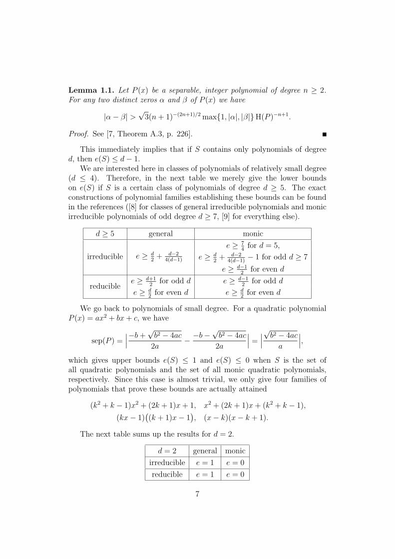
Lemma 1.1. Let P (x) be a separable, integer polynomial of degree n ≥ 2.For any two distinct zeros α and β of P (x) we have

|α− β| >√

3(n+ 1)−(2n+1)/2 max{1, |α|, |β|}H(P )−n+1.

Proof. See [7, Theorem A.3, p. 226].

This immediately implies that if S contains only polynomials of degreed, then e(S) ≤ d− 1.

We are interested here in classes of polynomials of relatively small degree(d ≤ 4). Therefore, in the next table we merely give the lower boundson e(S) if S is a certain class of polynomials of degree d ≥ 5. The exactconstructions of polynomial families establishing these bounds can be foundin the references ([8] for classes of general irreducible polynomials and monicirreducible polynomials of odd degree d ≥ 7, [9] for everything else).

d ≥ 5 general monic

irreducible e ≥ d2

+ d−24(d−1)

e ≥ 74

for d = 5,

e ≥ d2

+ d−24(d−1)

− 1 for odd d ≥ 7

e ≥ d−12

for even d

reduciblee ≥ d+1

2for odd d e ≥ d−1

2for odd d

e ≥ d2

for even d e ≥ d2

for even d

We go back to polynomials of small degree. For a quadratic polynomialP (x) = ax2 + bx+ c, we have

sep(P ) =∣∣∣−b+

√b2 − 4ac

2a− −b−

√b2 − 4ac

2a

∣∣∣ =∣∣∣√b2 − 4ac

a

∣∣∣,which gives upper bounds e(S) ≤ 1 and e(S) ≤ 0 when S is the set ofall quadratic polynomials and the set of all monic quadratic polynomials,respectively. Since this case is almost trivial, we only give four families ofpolynomials that prove these bounds are actually attained

(k2 + k − 1)x2 + (2k + 1)x+ 1, x2 + (2k + 1)x+ (k2 + k − 1),

(kx− 1)((k + 1)x− 1

), (x− k)(x− k + 1).

The next table sums up the results for d = 2.

d = 2 general monic

irreducible e = 1 e = 0

reducible e = 1 e = 0

7

For cubic polynomials, the case of general (i.e. nonmonic) polynomialswas first solved by Evertse [15] and later Schonhage [32] gave an easier con-structive proof. In the monic case Bugeaud and Mignotte [9] proved thelower bound e(M3) ≥ 3

2, where M3 is the set of monic cubic polynomials

with integer coefficients. They also showed that e(M3) = 32

is equivalentto Hall’s conjecture which asserts that, for any positive real number ε, wehave |x3 − y2| > x1/2−ε, for any suficiently large positive integers x and ywith x3 6= y2. Hall’s conjecture is one of the many consequences of theabc-conjecture (see [30]).

Proving that e(RM3) = 1 is not hard when we notice that a polynomialfrom this set is a product of a linear and a quadratic polynomial, both monicand with integer coefficients because of Gauss’s Lemma 0.1. In the next tablewe summarize known results for d = 3:

d = 3 general monic

irreducible e = 2 e ≥ 32

reducible e = 2 e = 1

Until now no exact values when d = 4 were known, just the lower boundsgiven in the following table:

d = 4 general monic

irreducible e ≥ 136

e ≥ 32

reducible e ≥ 73

e ≥ 2

The bound for the nonmonic irreducible case arises from a general construc-tion by Bugeaud and Dujella [8] which gives e((P 4,n(x))n∈N) = 13

6in this

special case, where

P 4,n(x) = (20n4 − 2)x4 + (16n5 + 4n)x3 + (16n6 + 4n2)x2 + 8n3x+ 1.

For nonmonic reducible polynomials, a recent unpublished result by Bugeaudand Dujella, shows that the sequence

P4,n(x) =((2n+ 1)x3 + (2n− 1)x2 + (n− 1)x− 1

)((n2 + 3n+ 1)x− (n+ 2)

)gives e ≥ e((P4,n(x))n∈N) = 7

3. The bound for monic irreducible polynomials

e ≥ 32

is deduced by looking at the sequence

P4,n(x) = (x2 − nx+ 1)2 − 2(nx− 1)2, n ∈ N

(see Bugeaud and Mignotte [9]). Finally, for reducible monic polynomials,it follows from a general case discussed in [9] that e(RM4) ≥ 2. While

8

the proof from [9] is nonconstructive, in Section 1.2 we establish the sameinequality by exhibiting a set S ⊆ RM4 such that e(S) = 2. In Section 1.3we prove that e(RM4) ≤ 2. By putting together the results from Sections1.2 and 1.3, we obtain the main result of this chapter, which gives the firstexact value in the above table for d = 4.

Theorem 1.1. It holds that e(RM4) = 2.

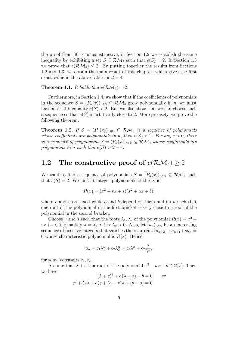
Furthermore, in Section 1.4, we show that if the coefficients of polynomialsin the sequence S = (Pn(x))n∈N ⊆ RM4 grow polynomially in n, we musthave a strict inequality e(S) < 2. But we also show that we can choose sucha sequence so that e(S) is arbitrarily close to 2. More precisely, we prove thefollowing theorem.

Theorem 1.2. If S = (Pn(x))n∈N ⊆ RM4 is a sequence of polynomialswhose coefficients are polynomials in n, then e(S) < 2. For any ε > 0, thereis a sequence of polynomials S = (Pn(x))n∈N ⊆ RM4 whose coefficients arepolynomials in n such that e(S) > 2− ε.

1.2 The constructive proof of e(RM4) ≥ 2

We want to find a sequence of polynomials S = (Pn(x))n∈N ⊆ RM4 suchthat e(S) = 2. We look at integer polynomials of the type

P (x) = (x2 + rx+ s)(x2 + ax+ b),

where r and s are fixed while a and b depend on them and on n such thatone root of the polynomial in the first bracket is very close to a root of thepolynomial in the second bracket.

Choose r and s such that the roots λ1, λ2 of the polynomial R(x) = x2 +rx+ s ∈ Z[x] satisfy λ = λ1 > 1 > λ2 > 0. Also, let (an)n∈N be an increasingsequence of positive integers that satisfies the recurrence an+2+ran+1+san =0 whose characteristic polynomial is R(x). Hence,

an = c1λn1 + c2λ

n2 = c1λ

n + c2s

λn,

for some constants c1, c2.Assume that λ + ε is a root of the polynomial x2 + ax + b ∈ Z[x]. Then

we have(λ+ ε)2 + a(λ+ ε) + b = 0 or

ε2 + (2λ+ a)ε+ (a− r)λ+ (b− s) = 0.

9

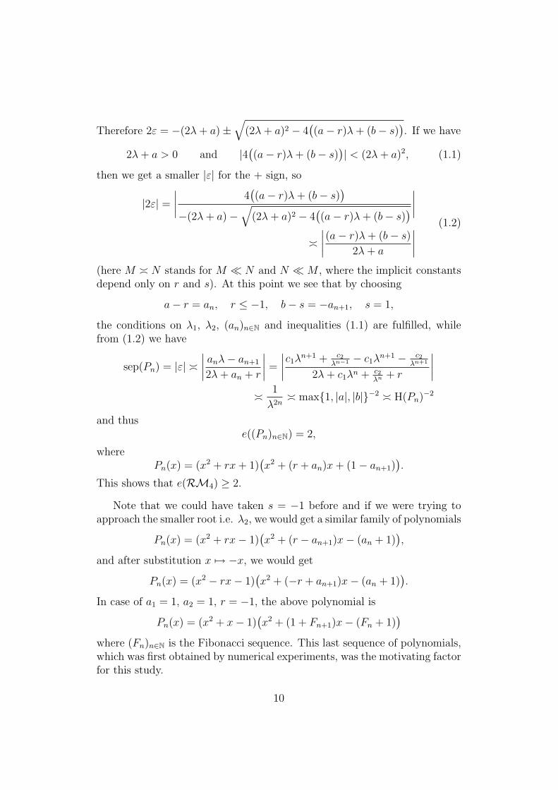
Therefore 2ε = −(2λ+ a)±√

(2λ+ a)2 − 4((a− r)λ+ (b− s)

). If we have

2λ+ a > 0 and |4((a− r)λ+ (b− s)

)| < (2λ+ a)2, (1.1)

then we get a smaller |ε| for the + sign, so

|2ε| =∣∣∣∣ 4

((a− r)λ+ (b− s)

)−(2λ+ a)−

√(2λ+ a)2 − 4

((a− r)λ+ (b− s)

)∣∣∣∣�∣∣∣∣(a− r)λ+ (b− s)

2λ+ a

∣∣∣∣(1.2)

(here M � N stands for M � N and N �M , where the implicit constantsdepend only on r and s). At this point we see that by choosing

a− r = an, r ≤ −1, b− s = −an+1, s = 1,

the conditions on λ1, λ2, (an)n∈N and inequalities (1.1) are fulfilled, whilefrom (1.2) we have

sep(Pn) = |ε| �∣∣∣∣ anλ− an+1

2λ+ an + r

∣∣∣∣ =

∣∣∣∣c1λn+1 + c2λn−1 − c1λn+1 − c2

λn+1

2λ+ c1λn + c2λn

+ r

∣∣∣∣� 1

λ2n� max{1, |a|, |b|}−2 � H(Pn)−2

and thuse((Pn)n∈N) = 2,

wherePn(x) = (x2 + rx+ 1)

(x2 + (r + an)x+ (1− an+1)

).

This shows that e(RM4) ≥ 2.

Note that we could have taken s = −1 before and if we were trying toapproach the smaller root i.e. λ2, we would get a similar family of polynomials

Pn(x) = (x2 + rx− 1)(x2 + (r − an+1)x− (an + 1)

),

and after substitution x 7→ −x, we would get

Pn(x) = (x2 − rx− 1)(x2 + (−r + an+1)x− (an + 1)

).

In case of a1 = 1, a2 = 1, r = −1, the above polynomial is

Pn(x) = (x2 + x− 1)(x2 + (1 + Fn+1)x− (Fn + 1)

)where (Fn)n∈N is the Fibonacci sequence. This last sequence of polynomials,which was first obtained by numerical experiments, was the motivating factorfor this study.

10

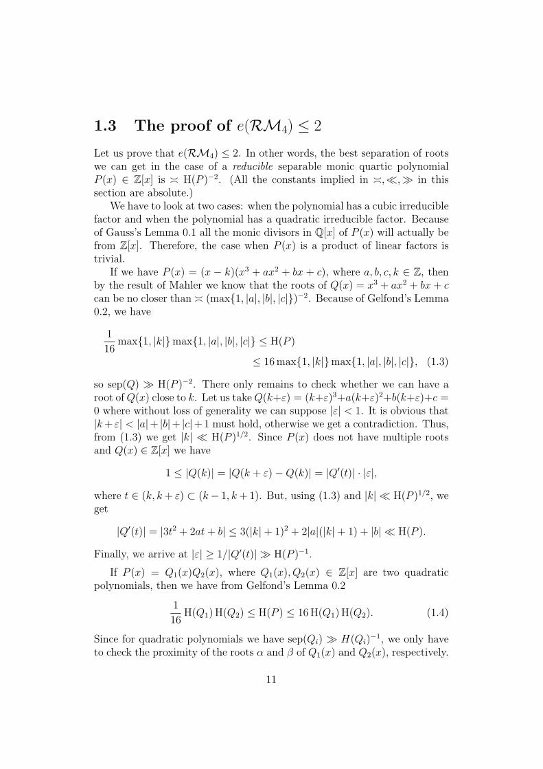
1.3 The proof of e(RM4) ≤ 2

Let us prove that e(RM4) ≤ 2. In other words, the best separation of rootswe can get in the case of a reducible separable monic quartic polynomialP (x) ∈ Z[x] is � H(P )−2. (All the constants implied in �,�,� in thissection are absolute.)

We have to look at two cases: when the polynomial has a cubic irreduciblefactor and when the polynomial has a quadratic irreducible factor. Becauseof Gauss’s Lemma 0.1 all the monic divisors in Q[x] of P (x) will actually befrom Z[x]. Therefore, the case when P (x) is a product of linear factors istrivial.

If we have P (x) = (x − k)(x3 + ax2 + bx + c), where a, b, c, k ∈ Z, thenby the result of Mahler we know that the roots of Q(x) = x3 + ax2 + bx+ ccan be no closer than � (max{1, |a|, |b|, |c|})−2. Because of Gelfond’s Lemma0.2, we have

1

16max{1, |k|}max{1, |a|, |b|, |c|} ≤ H(P )

≤ 16 max{1, |k|}max{1, |a|, |b|, |c|}, (1.3)

so sep(Q) � H(P )−2. There only remains to check whether we can have aroot ofQ(x) close to k. Let us takeQ(k+ε) = (k+ε)3+a(k+ε)2+b(k+ε)+c =0 where without loss of generality we can suppose |ε| < 1. It is obvious that|k+ ε| < |a|+ |b|+ |c|+ 1 must hold, otherwise we get a contradiction. Thus,from (1.3) we get |k| � H(P )1/2. Since P (x) does not have multiple rootsand Q(x) ∈ Z[x] we have

1 ≤ |Q(k)| = |Q(k + ε)−Q(k)| = |Q′(t)| · |ε|,

where t ∈ (k, k+ ε) ⊂ (k− 1, k+ 1). But, using (1.3) and |k| � H(P )1/2, weget

|Q′(t)| = |3t2 + 2at+ b| ≤ 3(|k|+ 1)2 + 2|a|(|k|+ 1) + |b| � H(P ).

Finally, we arrive at |ε| ≥ 1/|Q′(t)| � H(P )−1.

If P (x) = Q1(x)Q2(x), where Q1(x), Q2(x) ∈ Z[x] are two quadraticpolynomials, then we have from Gelfond’s Lemma 0.2

1

16H(Q1) H(Q2) ≤ H(P ) ≤ 16 H(Q1) H(Q2). (1.4)

Since for quadratic polynomials we have sep(Qi) � H(Qi)−1, we only have

to check the proximity of the roots α and β of Q1(x) and Q2(x), respectively.

11

Theorem A.1 from [7, p. 223] states that in our separable case

|α− β| ≥ 2−13−5/2 · H(Q1)−2 H(Q2)

−2 ·max{1, |α|}max{1, |β|} � H(P )−2.

Hence, we proved that e(RM4) ≤ 2, which concludes the proof of Theorem1.1.

1.4 Polynomial growth of coefficients

In Section 1.2 we exhibited a family of reducible monic polynomials Pn(x)whose coefficients grow exponentially in n such that sep(Pn) � H(Pn)−2.

We will show that this is not possible if the coefficients grow polynomi-ally. More precisely, let Pn(x) = P (n, x) ∈ Z[n, x] be a polynomial which ismonic of degree 4 in x and such that for every positive integer n′, polynomialPn′(x) ∈ Z[x] is reducible. This is the exact meaning of the conditions in thefirst statement of Theorem 1.2. Now we will need a quantitative version ofHilbert’s Irreducibility Theorem. Hilbert’s Irreducibility Theorem roughlyasserts that for polynomials in several variables irreducible over the ratio-nal field, there always exist rational specializations of some of the variableswhich preserve irreducibility [34]. Stating precisely, we will use the followingtheorem proved by Dorge [12].

Theorem H-D. If f(x1, . . . , xk, t) is an irreducible polynomial with integralcoefficients and if R(N) is the number of integers τ such that |τ | < N andf(x1, . . . , xk, τ) is reducible, then R(N) ≤ CN1−α where α, C are certainpositive constants.

Note that an earlier result by Skolem [33] giving limN→∞R(N)/N =0 would be sufficient for our purposes. Together with our assumption onreducibility this easily implies that

Pn(x) = Qn,1(x)Qn,2(x),

where Qn,1(x) and Qn,2(x) are monic polynomials in x whose coefficients areinteger polynomials in n. Note that because of the result in the previoussection, the case of a reducible monic polynomial with a linear factor is notvery interesting. Therefore, we will assume that Qn,1(x) and Qn,2(x) areirreducible quadratic polynomials in x without common roots, so we maywrite

Qn,1(x) = x2 + r(n)x+ s(n), Qn,2(x) = x2 + a(n)x+ b(n),

12

where r(n), s(n), a(n), b(n) ∈ Z[n]. For the sake of simplicity, we will usuallyomit n. As already mentioned, we can assume that the closest roots of P area root of Q1 and a root of Q2. So, without loss of generality, let us take

2 sep(P ) = 2ε = −r +√r2 − 4s+ a+

√a2 − 4b.

After some manipulation we get that ε satisfies the following equality

ε4 − 2(a− r)ε3 + (r2 + a2 − 3ra+ 2s+ 2b)ε2

− (a− r)(−ra+ 2s+ 2b)ε+ (s2 + b2 − rsa− rab− 2bs+ sa2 + br2) = 0.

(1.5)

Notice that the last term is just the resultant Resx(Q1, Q2) of the polynomialsQ1 and Q2:

Res(Q1, Q2) = Res(Q1, Q2 −Q1) = (b− s)2 + (a− r)(as− br).

Let us suppose that ε � H−2, where by Gelfond’s Lemma 0.2, H =H(P ) � H(Q1) H(Q2). We mention here that all the constants in O, �, �,� in the first part of this section depend at most on the coefficients of r, s, a, b.Since P (x) is a separable integer polynomial, it follows that Res(Q1, Q2) isan integer polynomial in n and |Res(Q1, Q2)| ≥ 1. Now we get from (1.5)and (1.4) that

H−2 � ε�|Res(Q1, Q2)|

| ε3︸︷︷︸O(H−6)

− 2(a− r)ε2︸ ︷︷ ︸O(H−3)

+ (r2 + a2︸ ︷︷ ︸O(H2)

− 3ra+ 2s+ 2b︸ ︷︷ ︸O(H)

)ε

︸ ︷︷ ︸O(1)

−(a− r)(−ra+ 2s+ 2b)|

and

H−2 � ε� |Res(Q1, Q2)||O(1)− 2as+ 2rb︸ ︷︷ ︸

O(H)

+ra2 − r2a+ 2rs− 2ab|. (1.6)

Because of Gelfond’s Lemma 0.2, |r|, |s|, |a|, |b| � H and |ar| � H whichimplies that |a| � H1/2 or |r| � H1/2. Without loss of generality we cansuppose that |a| � H1/2. Thus we get |ra2| = |ra| · |a| � H3/2 and |ab| =|a| · |b| � H3/2. We also have | − r2a+ 2rs| = |r| · |ra− 2s| = |r|O(H) so theinequality (1.6) becomes

H−2 � ε� 1

max{O(H3/2), |r|O(H)}.

13

It implies that |r| � H, so from |r| � H, we get |r| � H. Also, we obtain|Res(Q1, Q2)| = O(1). Since r, s, a, b are polynomials in n and |ra| � H,|rb| � H, we conclude that a and b are constants.

If we now have degn s < degn r, then

degn Res(Q1, Q2) = degn((b− s)2 + (a− r)(as− br)

)≥ degn r + degn s,

so |Res(Q1, Q2)| � H, which leads to a contradiction. Therefore, degn s =degn r and hence |s| � |r| � H→∞.

The leading coefficient of Res(Q1, Q2) as a polynomial in n, i.e. thecoefficient that belongs to the monomial of degree 2 degn r = 2 degn s, is theleading coefficient of s2 − ars + br2, i.e. k2

s − akrks + bk2r , where ks, kr are

leading coefficients of s and r, respectively. If it were 0, then −ks/kr ∈ Qwould be a root of x2 + ax+ b which is impossible, since by our assumptionthis polynomial is irreducible. Thus degn Res(Q1, Q2) = 2 degn r ≥ 2 andthis is in contradiction with the condition |Res(Q1, Q2)| = O(1).

We conclude that sep(Pn) � H(Pn)−2 cannot hold in this case, and thisproves the first statement of Theorem 1.2.

Although the previous result of this section shows that we cannot have afamily of reducible monic quartic integer polynomials with polynomial growthof coefficients that has the best possible exponent for root separation in thiscase, i.e. −2, we can still construct families with the exponent as close to −2as we like. The construction that follows is similar to the one in Section 1.2.

We look at the family of polynomials Pk,n(x) indexed with n ∈ N invariable x. As before, we will usually omit n and write simply Pk(x). Wedefine

Pk(x) = (x2 + nx+ 1)︸ ︷︷ ︸Qk(x)

(x2 + nx+ 1 + Ak+1x+ Ak)︸ ︷︷ ︸Rk(x)

= (x2 + n︸︷︷︸r

x+ 1︸︷︷︸s

)(x2 + (Ak+1 + n)︸ ︷︷ ︸

a

x+ (Ak + 1)︸ ︷︷ ︸b

),

where(Ak(n)

)k∈N0

is defined recursively by

A0(n) = 1, A1(n) = n, Ak+1(n) = nAk(n)− Ak−1(n) for n ≥ 2.

It is easy to see that degnAk = k, so we get (implied constants are absolutefrom now on)

H(Pk) � nk+2.

14

Let us look at the resultant:

Resx(Qk, Rk) = (b− s)2 − r(b− s)(a− r) + s(a− r)2

= A2k − nAkAk+1 + A2

k+1

= A2k + Ak+1(Ak+1 − nAk)

= A2k − Ak+1Ak−1

= A2k − (nAk − Ak−1)Ak−1

= Ak(Ak − nAk−1) + A2k−1

= A2k−1 − AkAk−2

= . . . = A21 − A2A0 = n2 − (n2 − 1) · 1 = 1.

(1.7)

The roots of Qk(x) are

α1 =−n−

√n2 − 4

2, α2 =

−n+√n2 − 4

2,

and the roots of Rk(x) are

β1 =−(Ak+1 + n)−

√(Ak+1 + n)2 − 4(Ak + 1)

2,

β2 =−(Ak+1 + n) +

√(Ak+1 + n)2 − 4(Ak + 1)

2.

Therefore,

α1 � −n, α2 � −1

n, β1 � −nk+1, β2 =

Ak + 1

β1

� −1

n,

so we have

1 = Res(Qk, Rk) = 1212 |α1 − β2|︸ ︷︷ ︸�n

|α1 − β1|︸ ︷︷ ︸�nk+1

|α2 − β1|︸ ︷︷ ︸�nk+1

sep(Pk),

and it follows that

sep(Pk) � n−2k−3 = n−2(k+2)n � H(Pk)−2+ 1

k+2 .

Hence, we proved the last statement of Theorem 1.2.

15

Chapter 2

General results on polynomialsin the p-adic setting

This chapter brings together results of a general nature on polynomials in thep-adic setting. These are for the most part analogues of the results in the realand complex case. In this way we streamline the proof of our main resultsand avoid unnecessary repetition. However, some lemmas on polynomialswhich are specific to the subject of a particular chapter are left there.

The first two lemmas give bounds on the size of roots and products ofroots of a polynomial.

Lemma 2.1. If α ∈ Cp is a root of the polynomial P (X) = anXn + · · · +

a1X + a0 ∈ Zp[X], then |a0|p ≤ |α|p ≤ 1/|an|p.

Proof. If α = 0, then both inequalities obviously hold. Therefore, we assumeα 6= 0. From P (α) = 0 we get

a0α−1 = −(anα

n−1 + · · ·+ a1).

If |α|p ≤ 1 this implies |a0α−1|p ≤ 1. If |α|p > 1, |a0α

−1|p ≤ 1 obviouslyholds. Either way, we get |a0|p ≤ |α|p and the other inequality follows fromthis one by noting that 1/α is a root of the polynomial XnP (1/X) = a0X

n+a1X

n−1 + · · ·+ an.

Lemma 2.2. Let P (X) = anXn+ · · ·+a1X+a0 = an(X−α1) · · · (X−αn) ∈

Cp[X]. Then for any set I ⊆ {1, . . . , n}, it holds∏i∈I

|αi|p ≤maxj∈{0,1,...,n} |aj|p

|an|p.

Proof. This is shown in [24, p. 341].

16

As an analogue of Lemma 1.1 proved by Mahler for complex roots, weprove a lower bound on the distance of two roots in the p-adic case. Just asin the complex case, for a polynomial P (x) of degree d ≥ 2 and with distinctroots α1, . . . , αd ∈ Cp, we set

sepp(P ) := min1≤i<j≤d

|αi − αj|p.

Lemma 2.3. Let P (X) be a separable, integer polynomial of degree n ≥ 2.For any two distinct zeros α, β ∈ Cp of P (X), we have

|α− β|p ≥ sepp(P ) ≥ n−32n H(P )−n+1.

First proof. First part of this proof has been done by Morrison (cf. [24]). Ifno two roots of the polynomial

P (X) = an(X−α1) · · · (X−αn) = anXn+· · ·+a1X+a0, αi ∈ Cp (1 ≤ i ≤ n)

are equal we look at the polynomial

Q(X) =∏

1≤i<j≤n

(X − (αi − αj)2

).

The coefficients of Q are symmetric polynomials with integer coefficients inα1, . . . , αn and therefore integer polynomials in elementary symmetric poly-nomials in α1, . . . , αn, that is, by Viete’s formulas, in a0

an, . . . , an−1

anand it is

easy to see that their degree in αi is at most 2(n − 1) and since each ofa0

an, . . . , an−1

anis of degree 1 in αi, we get that

a2n−2n Q(X) ∈ Z[a0, . . . , an−1, an][X] ⊂ Z[X].

According to Lemma 2.1, we now know that

|(αi − αj)2|p ≥ |constant term of a2n−2n Q(X)|p

and since

|constant term of a2n−2n Q(X)| = |a2n−2

n

∏1≤i<j≤n

(αi − αj)2| = |Disc(P )|

17

we are left to bound

|Disc(P )| =∣∣∣∣ 1

an(−1)

n(n−1)2 Res(P, P ′)

∣∣∣∣

=1

|an|| det

an · · · a0

. . . . . .

an · · · a0

nan · · · a1

. . . . . .

nan · · · a1

| = | det

1 · · · a0

. . . . . .

an · · · a0

n · · · a1

. . . . . .

nan · · · a1

|

≤ (n+ 1)n−1nn · nn H(P )2n−2 ≤ n3n H(P )2n−2.(2.1)

Finally, it follows that, sepp(P ) ≥ n−32n H(P )−n+1.

Second proof. We briefly sketch an alternative proof of this lemma. Insteadof using Morrison’s construction of the polynomial Q(X) from the first partof the proof we just showed, we use the procedure similar to what Mahleremployed in his proof of the complex numbers analogue of this result (cf. [7,Theorem A.3]). Namely,

|Disc(P )|p = |a2n−2n |p

∏1≤i<j≤n

|αi − αj|2p

≤ |α1 − α2|2p|an|2n−2p

∏1≤i<j≤n(i,j)6=(1,2)

(max{1, |αi|p}max{1, |αj|p}

)2≤ |α1 − α2|2p

(|an|p

∏1≤i≤n

max{1, |αi|})2n−2

≤ |α1 − α2|2p( max0≤i≤n

|ai|p)2n−2

≤ |α1 − α2|2p,

where we used Lemma 2.2 in order to get to the penultimate line.Combined with the upper bound (2.1) on |Disc(P )| from the first proof

and inequality1

|Disc(P )|≤ |Disc(P )|p,

we get another proof of Lemma 2.3.

The following lemma compares the value of an integer polynomial at somenumber with the distance of this number from the roots of the polynomial.

18

Lemma 2.4. Let P (X) be a non-constant, separable, integer polynomial ofdegree n. Let ξ ∈ Cp and α be a root of P (X) in Cp such that |ξ − α|p isminimal. Then

n−3n/2 H(P )−n+1|ξ − α|p ≤ |P (ξ)|p.

Proof. (cf. [7, Lemma A.8, p. 231]) Let P (X) = anXn + · · · + a1X + a0 =

an(X − α1) · · · (X − αn) ∈ Z[X], where we order the roots α1, . . . , αn ∈ Cp

in such a way that

α = α1 and |ξ − α1|p ≤ · · · ≤ |ξ − αn|p.

First we bound the discriminant of P (X) as in (2.1)

|Disc(P )| ≤ n3n H(P )2n−2.

Now we have,

n−3n/2 H(P )−n+1 ≤√|Disc(P )|p = |an|p|α1−α2|p · · · |α1−αn|p

√|Disc(Q)|p,

where Q(X) = an(X − α2) · · · (X − αn). Applying Lemma 2.2 to the integerpolynomial P (X), we get the last bound below

√|Disc(Q)|p = |an|n−2

p · |

∣∣∣∣∣∣∣α0

2 · · · αn−22

.... . .

...

α0n · · · αn−2

n

∣∣∣∣∣∣∣ |p≤ |an|n−2

p

∏2≤i≤n

max{1, |αi|p}n−2 ≤ 1.

Using |ξ − α1|p ≤ · · · ≤ |ξ − αn|p, we get for 1 ≤ i < j ≤ n

|αi − αj|p ≤ max{|ξ − αi|p, |ξ − αj|p} = |ξ − αj|pwhich combined with the previous bound gives

n−3n/2 H(P )−n+1 ≤ |an|p|ξ − α2|p · · · |ξ − αn|p,n−3n/2 H(P )−n+1|ξ − α|p ≤ |P (ξ)|p.

Next lemma gives a useful lower estimate for the distance between twodistinct algebraic numbers.

Lemma 2.5. Let α and β be distinct algebraic numbers in Cp of degree atmost m and n, respectively. Then there exists a positive constant c(m,n) < 1,depending only on m and n, such that

|α− β|p ≥ c(m,n) H(α)−n H(β)−m.

An admissible value for c(m,n) is (m+ 1)−n(n+ 1)−m.

19

Proof. If α and β are conjugate over Q, let their minimal polynomial overZ be P (X) = ak(X − α1) · · · (X − αk), where α1 = α, α2 = β. Thus,H(α) = H(β) = H(P ) and k ≤ min{m,n}. We are now in the situation ofLemma 2.3 and so

|α− β|p ≥ k−3k/2 H(P )−k+1 ≥ (m+ 1)−n(n+ 1)−m H(α)−n H(β)−m.

Next, we assume that numbers α and β are not conjugate over Q. Supposethat α and β are algebraic numbers of degree exactly m and n, respectively.Let

P (X) = am(X − α1) · · · (X − αm) = amXm + · · ·+ a1X + a0 and

Q(X) = bn(X − β1) · · · (X − βn) = bnXn + · · ·+ b1X + b0

be the minimal polynomials of α = α1 and β = β1 over Z. Then the resultantRes(P,Q) is a non-zero integer and it can be bounded from above:

|Res(P,Q)| = | det

am · · · a0

. . . . . .

am · · · a0

bn · · · b0. . . . . .

bn · · · b0

|

≤ (m+ 1)n(n+ 1)m H(P )n H(Q)m

= (m+ 1)n(n+ 1)m H(α)n H(β)m.

On the other hand, from the definition of Res(P,Q) we get

|Res(P,Q)|p = |bn|mp∏

1≤j≤n

|P (βj)|p

≤ |bn|mp |P (β)|p∏

2≤j≤n

(max

0≤i≤m|ai|p(max{1, |βj|p})m

)≤ |bn|mp |am|p|β − α|p

∏2≤i≤m

|β − αi|p∏

2≤j≤n

(max{1, |βj|p})m

≤ |bn|mp |am|p|β − α|p∏

2≤i≤m

(max{1, |αi|p}max{1, |β|p})∏

2≤j≤n

(max{1, |βj|p})m

≤ |β − α|p(|am|p

∏2≤i≤m

max{1, |αi|p})(|bn|p

∏1≤j≤n

max{1, |βj|p})m.

20

Lemma 2.2 together with the already used fact that all the coefficients of thepolynomials P (X) and Q(X) are integers implies that both brackets aboveare ≤ 1. Thus

|β−α|p ≥ |Res(P,Q)|p ≥1

|Res(P,Q)|≥ (m+1)−n(n+1)−m H(α)−n H(β)−m.

We immediately see that if the degrees of α and β are smaller than m andn, the same inequality holds a fortiori.

After covering both cases, this lemma is proved.

21

Chapter 3

On separation of roots in thep-adic case

3.1 General degree

Lemma 2.3 shows that for an integer polynomial P (X) of degree ≤ n, thedistance between two of its roots in Cp is always � H(P )−n+1, where theimplicit constant depends only on n. In the first part of this chapter we giveexplicit families of integer polynomials of general degree with close roots inCp. The second part deals with quadratic and especially cubic polynomialswith close roots.

One usual idea for construction of such polynomials is to take an alreadyknown family (Pk(X))k≥1 of polynomials whose coefficients are polynomialsin the indexing variable k, substitute k with 1/pk in Pk(X) and then multi-ply this polynomial with a sufficiently high power of pk so that the resultingpolynomial has integer coefficients. While the starting polynomial had rel-atively small discriminant, we arrive at a polynomial whose discriminant isa rational integer divisible by a large power of p and from Lemma 0.4 weexpect that such a polynomial has close roots in Cp. In order to find outhow small sepp really is, we use the so called Newton polygons. We brieflyexplain some basic facts on this concept adopting the exposition from [16]while more properties together with proofs can be found e.g. in [16, §6.4] or[17, §IV.3].

Let P (X) ∈ Cp[X] be a polynomial. Since we are interested in under-standing zeros of P (X), we may factor out the highest power of X whichdivides P (X). In other words, we may assume that P (0) 6= 0 and afterdividing by P (0), we may also assume that P (0) = 1. Thus, we take a

22

polynomialP (X) = 1 + a1X + a2X

2 + · · ·+ anXn

with ai ∈ Cp. In the Cartesian coordinate plane we plot the points (0, 0) and,for each i between 1 and n, (i, vp(ai)), where vp(x) = − logp(|x|p) is the usualp-adic valuation. If ai = 0 for some i, we take vp(ai) to be +∞ and think ofthe corresponding point as “infinitely high”. In practice, we just ignore thatvalue of i. The polygon we want to consider is the lower boundary of theconvex hull of this set of points. We can also think of it this way:

i) Start with the vertical half-line which is the negative part of y-axis.

ii) Rotate that line counter-clockwise until it hits one of the points wehave plotted.

iii) “Break” the line at that point, and continue rotating the remainingpart until another point is hit.

iv) Continue until all the points have either been hit or lie strictly abovea portion of the polygon. Cut off the polygon at its last vertex.

The resulting polygon is called Newton polygon of the polynomial P (X) withrespect to p. Since we always fix the prime p, we will usually not make areference to it. We will be interested in the following information from thispolygon:

i) the slopes of the line segments appearing in the polygon;

ii) the “length” of each slope, meaning the length of the projection of thecorresponding segment on the x-axis;

iii) the “breaks”, i.e. the values of i such that the point (i, vp(ai)) is avertex of the polygon.

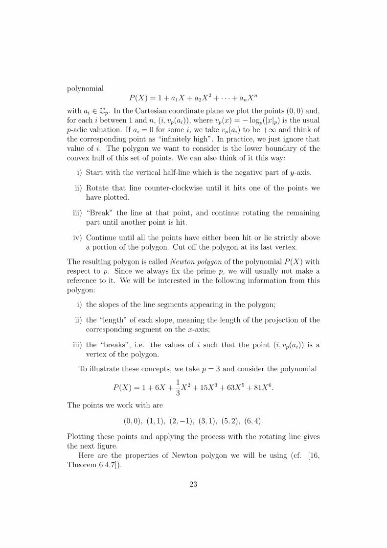
To illustrate these concepts, we take p = 3 and consider the polynomial

P (X) = 1 + 6X +1

3X2 + 15X3 + 63X5 + 81X6.

The points we work with are

(0, 0), (1, 1), (2,−1), (3, 1), (5, 2), (6, 4).

Plotting these points and applying the process with the rotating line givesthe next figure.

Here are the properties of Newton polygon we will be using (cf. [16,Theorem 6.4.7]).

23

Lemma 3.1. Let P (X) = 1 + a1X + a2X2 + · · · + anX

n ∈ Cp[X] be apolynomial, and let m1,m2, . . . ,mr be the slopes of its Newton polygon inincreasing order. Let i1, i2, . . . , ir be the corresponding lengths. Then, foreach k, 1 ≤ k ≤ r, P (X) has exactly ik roots in Cp (counting multiplicities)of p-adic absolute value pmk .

Thus, the polynomial from our example above has in C3 two roots ofabsolute value 1/

√3, three roots of absolute value 3 and one root of absolute

value 9.Getting back to our subject, here are some examples of polynomials with

small root separation. Note that the first two families are reducible, whilethe other two are irreducible according to Eisenstein’s criterion.

If we take P (X) =

(X − pk)(Xn−1 −X + pk)

(X − pk)(pkXn−1 −X + pk)

Xn − 2(X − pk)2

p2kXn − 2(X − pk)2

, k ≥ 1,

we get sepp(P )�

H(P )−

n−12

H(P )−n2

H(P )−n4

H(P )−n4− 1

2

. Let us show how to arrive at these results.

P (X) = (X − pk)(Xn−1 −X + pk)

One root of P (X) is pk, let another one, closest to pk, be pk + ε ∈ Cp. Then

P (pk + ε) = ε((pk + ε)n−1 − (pk + ε) + pk

)= 0,

24

and since ε 6= 0, we get (pk + ε)n−1 − ε = 0. Let us look at the polynomial

Q(X) =(pk +X)n−1 −X

p(n−1)k

= 1 +(n− 1)p(n−2)k − 1

p(n−1)kX +

(n− 1)(n− 2)

2· 1

p2kX2 + · · ·+ 1

p(n−1)kXn−1

= 1 +n−1∑i=1

aiXi.

If we now look at the Newton polygon of Q(X), we are interested in thepoints

(0, 0), (1, vp(a1)), (2, vp(a2)), . . . , (n− 1, vp(an−1)), i.e.

(0, 0), (1, vp

((n− 1)p(n−2)k − 1

p(n−1)k

)),

(2, vp

((n− 1)(n− 2)

2p2k

), . . . , (n− 1, vp

( 1

p(n−1)k

)).

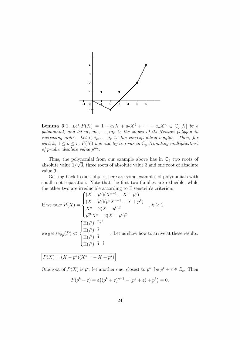
We see that vp(a1) = −(n − 1)k, vp(ai) ≥ −ik for i = 2, . . . , n − 2 andvp(an−1) = −(n − 1)k. Therefore, the Newton polygon is as shown in thepicture below.

From the properties of Newton polygons i.e. Lemma 3.1, as there isexactly one slope λ = −(n−1)k−0

1−0= −(n− 1)k of length 1 and the other slope

λ = 0 is of length n−2, we conclude that exactly one root ξ of Q(X) satisfies|ξ|p = p−(n−1)k and all the other roots η of Q(X) have |η|p = 1. The choiceof ε implies that ε = ξ so

sepp(P ) ≤ |ε|p = p−(n−1)k = (p2k)−n−1

2 =(

H(P ))−n−1

2 .

25

The case of the polynomial P (X) = (X − pk)(pkXn−1 −X + pk) is donevery similarly. We omit the details.

P (X) = Xn − 2(X − pk)2

The polynomial P (X) is irreducible over Q because of Eisenstein’s criterion.Let pk + ε be the root of P (X) closest to pk. Then

P (pk + ε) = (pk + ε)n − 2((pk + ε)− pk

)2= (pk + ε)n − 2ε2 = 0.

For the polynomial

Q(X) =1

pnk((pk +X)n − 2X2

)= 1 +

n

pkX +

(n2

)p(n−2)k − 2

pnkX2 +

(n3

)p3k

X3 + · · ·+ 1

pnkXn

= 1 +n∑i=1

aiXi,

we have vp(ai) ≥ −ik, for i = 1 and i = 3, . . . , n− 1, and vp(a2) = vp(an) =−nk. Therefore, the Newton polygon of Q(X) is as shown below.

Since there are two slopes on it, λ = −nk2

of length 2 and λ = 0 of lengthn − 2, we conclude that there are two roots of Q(X) with p-adic absolute

value p−nk2 and these have to be ε and −ε. Finally we get

sepp(P ) ≤ |(pk+ε)−(pk−ε)|p = |2ε|p = |ε|p = p−nk2 = (p2k)−

n4 �

(H(P )

)−n4 .

Although we tacitly used that p is an odd prime, note that for p = 2we can take P (X) = Xn − 3(X − pk)2 and all the conclusions remain the

26

same. Also, compare with Lemma 5.1 for a more detailed analysis of a similarpolynomial.

The case of the polynomial P (X) = p2kXn − 2(X − pk)2 is done verysimilarly and we again leave the details to the interested reader.

3.2 Degrees two and three

Quadratic polynomials

Lemma 2.3 says that for a quadratic separable polynomial P (X) with integercoefficients, we have sepp(P ) ≥ 1

8H(P )−1. To show that the exponent−1 over

H(P ) really can be attained we can take the family of reducible polynomials

Pk(X) = X(X + pk) = X2 + pkX, k ≥ 1

which gives sepp(Pk) = p−k = H(P )−1. We can also look at the family ofirreducible polynomials

Pk(X) = (−p2k + pk + 1)X2 + (p2k + 2pk)X + p2k, k ≥ 1

for which

sepp(Pk) =

∣∣∣∣√

(p2k + 2pk)2 − 4(−p2k + pk + 1)p2k

−p2k + pk + 1

∣∣∣∣p

=

∣∣∣∣√

5p4k

−p2k + pk + 1

∣∣∣∣p

= p−2k

if p 6= 5. Thus, here we have sepp(Pk) � H(Pk)−1, where the implied con-

stants are absolute. The last asymptotic relation obviously holds even ifp = 5. For a family of monic irreducible quadratic polynomials (Pk(X))kwith root separation sepp(Pk) � H(Pk)

−1, see Lemma 5.2.

Lemma 3.2. Let P (X) be a quadratic separable polynomial with integer co-efficients. For every prime p, we have

sepp(P ) ≥ 1

H(P )√

5.

Equality is achieved if and only if p = 5 and P (X) ∈ {X2 ±X + 1,−X2 ±X − 1}.

27

Proof. For a separable quadratic polynomial P (X) = aX2 + bX + c withinteger coefficients, the following sequence of inequalities holds

sepp(P ) =

∣∣∣∣√b2 − 4ac

a

∣∣∣∣p

=|b2 − 4ac|

12p

|a|p

(i)

≥ 1

|b2 − 4ac| 12(ii)

≥ 1(|b|2 + 4|a||c|

) 12

(iii)

≥ 1

H(P )√

5.

(3.1)In (3.1.i) equality holds if and only if p does not divide a and b2 − 4ac = pk

for some nonnegative integer k. In (3.1.ii) equality is achieved if and onlyif ac ≤ 0 while equality in (3.1.iii) is equivalent to |a| = |b| = |c| = H(P ).Combining these conditions we arrive at the statement of the lemma.

Reducible cubic case

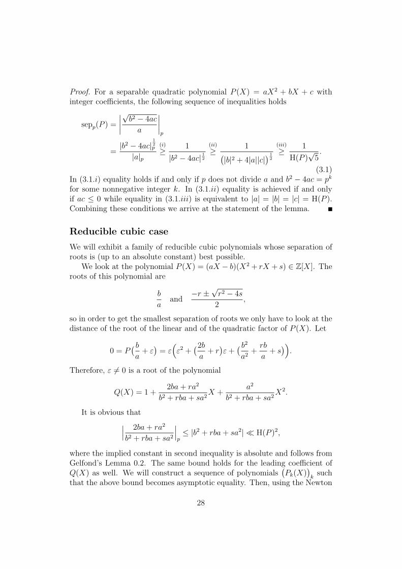
We will exhibit a family of reducible cubic polynomials whose separation ofroots is (up to an absolute constant) best possible.

We look at the polynomial P (X) = (aX − b)(X2 + rX + s) ∈ Z[X]. Theroots of this polynomial are

b

aand

−r ±√r2 − 4s

2,

so in order to get the smallest separation of roots we only have to look at thedistance of the root of the linear and of the quadratic factor of P (X). Let

0 = P( ba

+ ε)

= ε(ε2 +

(2b

a+ r)ε+

( b2a2

+rb

a+ s)).

Therefore, ε 6= 0 is a root of the polynomial

Q(X) = 1 +2ba+ ra2

b2 + rba+ sa2X +

a2

b2 + rba+ sa2X2.

It is obvious that∣∣∣ 2ba+ ra2

b2 + rba+ sa2

∣∣∣p≤ |b2 + rba+ sa2| � H(P )2,

where the implied constant in second inequality is absolute and follows fromGelfond’s Lemma 0.2. The same bound holds for the leading coefficient ofQ(X) as well. We will construct a sequence of polynomials

(Pk(X)

)k

suchthat the above bound becomes asymptotic equality. Then, using the Newton

28

polygons it will follow that sep(Pk) � H(Pk)−2 which is, of course, the best

possible exponent.To this end we will use the sequence

(Ak(n)

)k≥0

of polynomials definedrecursively

A0(n) = 1, A1(n) = n, Ak+1(n) = nAk(n)− Ak−1(n) for n ≥ 2.

We already used this sequence in the real case of reducible quartics. It iseasy to see that degnAk = k, and it was shown in (1.7) that

A2k − nAkAk+1 + A2

k+1 = 1.

Now we define new polynomials Ak(n) by “reversion”: Ak(n) = nkAk(

1n

). It

is a recursive sequence

A0(n) = 1, A1(n) = n, Ak+1(n) = Ak(n)− n2Ak−1(n) for n ≥ 2

that satisfiesA2k+1 − Ak+1Ak + n2A2

k = (nk+1)2. (3.2)

First few terms of the sequence Ak(n) are

1, 1,−n2 + 1,−2n2 + 1, n4 − 3n2 + 1, 3n4 − 4n2 + 1, . . .

so we see that the constant term is always 1 and the degree is degn Ak = 2⌊k2

⌋.

Fixing any integer k ≥ 2, we set

ak,l = Ak(pl), bk,l = Ak+1(p

l), rk,l = −1, sk,l = p2l, for l ≥ 1.

Denoting

Pk,l(X) = (ak,lX − bk,l)(X2 + rk,lX + sk,l)

=(Ak(p

l)X − Ak+1(pl))(X2 −X + p2l), l ≥ 1,

we see that the quadratic factor is irreducible over Q and (dropping indicesk and l)

vp

( 2ba+ ra2

b2 + rba+ sa2

)= −2(k + 1)l

since a ≡ b ≡ 1 (mod p) and b2 + rba + sa2 = p2(k+1)l because of (3.2).Therefore, |ε|p = p−2(k+1)l and since |a| �k p2bk/2cl and |b| �k p2b(k+1)/2cl, wehave

H(Pk) �k p2(b(k+1)/2c+1)l,

which impliessepp(Pk,l)� H(Pk,l)

−2+εk , l→∞.Here, εk → 0 when k → ∞. Hence, we can choose Pk(X) = Pk,lk(X) forsome sequence (lk)k which increases sufficiently fast so that

sepp(Pk) � H(Pk)−2, k →∞.

29

Irreducible cubic case

Let P (X) = aX3 + bX2 + cX + d ∈ Z[X] be an integer polynomial withdistinct roots α1, α2, α3 ∈ Cp. In order to analyze sepp(P ), we first constructa polynomial whose roots are closely related to the distances between theroots of P (X). Denoting by Q(X) = ResY

(P (Y ), P (X + Y )), Lemma 0.4

tells us that Q(X) has integer coefficients and for x0 ∈ Cp:

Q(x0) = 0 ⇔ P (Y ) and P (x0 + Y ) have a common root in Cp

⇔ ∃y0 ∈ Cp such that P (y0) = P (x0 + y0) = 0

⇔ ∃α, β ∈ Cp such that P (α) = P (β) = 0, x0 = α− β

This shows that if we denote δ1 = α1 − α2, δ2 = α2 − α3, δ3 = α3 − α1, then

Q(X) = a∏

1≤i≤31≤j≤3

(X − (αi − αj)

)= a(X2 − δ2

1)(X2 − δ22)(X2 − δ2

3)X3.

Taking R(X) = Q(X)/X3 ∈ Z[X] and then S(X) = R(√X)/R(0), we get

that

S(X) =−1

δ21δ

22δ

23

(X − δ21)(X − δ2

2)(X − δ23)

is a polynomial in Q[X] such that

S(0) = 1 and sepp(P ) = min{|δ|

12p : δ ∈ Cp, S(δ) = 0

}. (3.3)

After some computation, we obtain

S(X) = 1− (b2 − 3ac)2X

b2c2 − 4ac3 − 4b3d+ 18abcd− 27a2d2

+2a2 (b2 − 3ac)X2

b2c2 − 4ac3 − 4b3d+ 18abcd− 27a2d2

− a4X3

b2c2 − 4ac3 − 4b3d+ 18abcd− 27a2d2. (3.4)

Before announcing the family of polynomials with the best currentlyknown upper bound for separation of roots, let us mention an example we getusing the process described in the introduction of this chapter. Taking from[8] a family of polynomials Qk(X) = (8k3−2)X3 + (4k4 + 4k)X2 + 4k2X+ 1,k ≥ 1, with close roots in R, substituting k with 1/pk and multiplying by p4k

we procure the polynomial

Pk(X) = (−2p4k + 8pk)X3 + (4p3k + 4)X2 + (4p2k)X + p4k

30

and insert its coefficients into (3.4). The coefficients of S(X) = a0 + a1X +a2X

2 + a3X3 in the order a0, a1, a2, a3 are

1,16p−13k

(2− 8p3k + 5p6k

)2−8 + 27p3k

,

−16p−11k

(−4 + p3k

)2 (2− 8p3k + 5p6k

)−8 + 27p3k

,4p−9k

(−4 + p3k

)4−8 + 27p3k

,

which gives the following points we are interested in (for p 6= 2)

(0, vp(a0)), (1, vp(a1)), (2, vp(a2)), (3, vp(a3))

= (0, 0), (1,−13k), (2,−11k), (3,−9k).

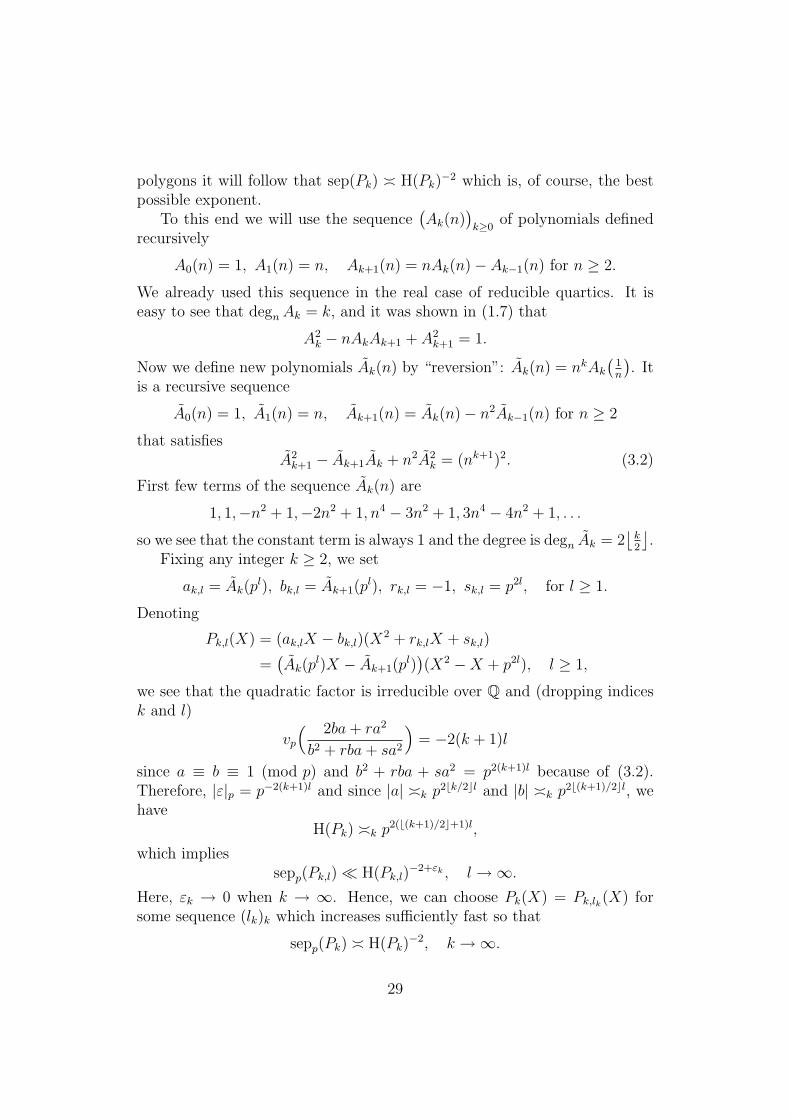
Thus, the Newton polygon of S(X) is as below (note that we have droppedthe index k to ease the notation, but this is still a family of polynomials).

Lemma 3.1 and (3.3) show that sepp(Pk) = p−13k/2 � H(Pk)−13/8 because

H(Pk) � p4k.Finally, for a family of polynomials

Pk(X) = (−45056pk−17280p4k−243p7k)X3 +(8192+1536p3k−378p6k)X2

+ (512p2k + 156p5k)X + 8p4k + 2p7k,

31

coefficients of S(X) = a0 + a1X + a2X2 + a3X

3 in the order a0, a1, a2, a3 are

1,256p−25k

(2097152 + 9p3k

(327680 + 99p3k

(1536 + 256p3k + 9p6k

)))219683 (128 + 81p3k)

,

−16p−23k

(45056 + 27p3k

(640 + 9p3k

))219683 (128 + 81p3k)

·

·(2097152 + 9p3k

(327680 + 99p3k

(1536 + 256p3k + 9p6k

))),

p−21k(45056 + 27p3k

(640 + 9p3k

))478732 (128 + 81p3k)

,

which gives the following points we are interested in (for p 6= 2)

(0, vp(a0)), (1, vp(a1)), (2, vp(a2)), (3, vp(a3))

= (0, 0), (1,−25k), (2,−23k), (3,−21k).

Lemma 3.1 and (3.3) show that sepp(Pk) = p−25k/2 � H(Pk)−25/14 because

H(Pk) � p7k. Even if asymptotics does not change for p = 2, we are notcertain that the polynomials Pk(X) are irreducible in this case. For p 6= 2this is guaranteed by Eisenstein’s criterion.

Remark 3.1. This last family of polynomials was deduced from the family

(−45056n6 − 17280n3 − 243)X3 + (8192n7 + 1536n4 − 378n)X2

+ (512n5 + 156n2)X + 8n3 + 2, n ≥ 0

by the usual process. The original family of polynomials gives a separationof roots in the real case with the exponent −25/14 which is at present thebest exponent for a family of irreducible cubic polynomials with polynomialgrowth of coefficients. Although Schonhage [32] proved that in the real casethe best possible exponent −2 is attainable, his families of polynomials haveexponential growth of coefficients. One of the main ingredients Schonhageused to construct these families is continued fraction expansion of real num-bers. In the p-adic setting there are several types of continued fractions thathave been proposed. None of them have all the good properties of the stan-dard continued fractions and at the moment Schonhage’s construction doesnot seem to translate easily to p-adic numbers. This is one of the reasonswhy we are interested in families of polynomials with polynomial growth ofcoefficients.

32

Chapter 4

p-adic T -numbers

4.1 Introduction

Mahler [20] introduced in 1932 a classification of complex transcendentalnumbers according to how small the value of an integer polynomial at thegiven number can be with regards to the the height and degree of this poly-nomial. In 1939 Koksma [18] devised another classification which looks athow closely the complex transcendental number can be approximated by al-gebraic numbers of bounded height and degree. Koksma proved that thetwo classifications are identical and thus we have three classes consisting ofS-numbers or S∗-numbers, T -numbers or T ∗-numbers and U -numbers or U∗-numbers. Here the nonstared letters refer to Mahler’s classification whereasthe stared ones refer to Koksma’s. See [7] for all references.

While almost all numbers in the sense of Lebesgue measure are S-numbersand U -numbers contain for example Liouville numbers, it was only in 1968that Schmidt [29] proved the existence of T -numbers.

Schlickewei [28] adapted this result to the p-adic setting. After this infor-mal introduction, we give the necessary definitions in order to explain howthe main result of this chapter improves Schlickewei’s result. We take inspi-ration from a paper by R. C. Baker [1] on complex T -numbers in order toestablish similar results for p-adic T -numbers.

In analogy with his classification of complex numbers, Mahler proposed aclassification of p-adic numbers. Let ξ ∈ Qp and given n ≥ 1, H ≥ 1, definethe quantity

wn(ξ,H) := min{|P (ξ)|p : P (X) ∈ Z[X], deg(P ) ≤ n, H(P ) ≤ H, P (ξ) 6= 0}.We set

wn(ξ) := lim supH→∞

− log(Hwn(ξ,H))

logHand w(ξ) := lim sup

n→∞

wn(ξ)

n,

33

and thus wn(ξ) is the upper limit of the real numbers w for which there existinfinitely many integer polynomials P (X) of degree at most n satisfying

0 < |P (ξ)|p ≤ H(P )−w−1.

In analogy with Koksma’s classification of complex numbers, for ξ ∈ Qp

and given n ≥ 1, H ≥ 1, we define the quantity

w∗n(ξ,H) := min{|ξ−α|p : α algebraic in Qp, deg(α) ≤ n, H(α) ≤ H, α 6= ξ}.

We set

w∗n(ξ) := lim supH→∞

− log(Hw∗n(ξ,H))

logHand w∗(ξ) := lim sup

n→∞

w∗n(ξ)

n,

and thus w∗n(ξ) is the upper limit of the real numbers w for which there existinfinitely many algebraic numbers α in Qp of degree at most n satisfying

0 < |ξ − α|p ≤ H(α)−w−1.

We say that a transcendental number ξ ∈ Qp is an

• S-number if 0 < w(ξ) <∞;

• T -number if w(ξ) =∞ and wn(ξ) <∞ for any integer n ≥ 1;

• U-number if w(ξ) =∞ and wn(ξ) =∞ for some integer n ≥ 1.

S∗-, T ∗- and U∗- numbers are defined as above, using w∗n in place of wn.Actually, the definition of the quantity wn(ξ) given here differs from the

one used by Schlickewei [28]. Indeed, for him, the numerator of the definingfraction is − log(wn(ξ,H)) instead of − log(Hwn(ξ,H)). This means thatthere is a shift by 1 in the value of the critical exponent, which however doesnot imply any change regarding the class of a given p-adic number. We haveadopted the same notation as in [7] since then wn(ξ) = w∗n(ξ) = n holds foralmost all p-adic numbers ξ, with respect to the Haar measure on Qp.

Another possible issue is also settled, namely, as in the real case, ifw∗n(ξ,H) is replaced by the minimum of |ξ − α|p over all numbers α 6= ξwhich are roots of integer polynomials of degree at most n and height atmost H, the value of w∗n(ξ) does not change, see [7, §9.3]. So by replacingQp with an algebraic closure Qp in the definition of w∗n(ξ,H) we gain noth-ing new in respect to w∗n(ξ). See [7] for details and further results on theexponents wn and w∗n.

The central result of Schlickewei’s paper [28] is his Theorem 2:

34

Theorem S. Let (Bn)n≥1 be a sequnce of real numbers such that

B1 > 9, Bn > 3n2Bn−1 for n > 1.

There exist numbers ξ ∈ Qp with

w∗n(ξ) = Bn for any n ≥ 1.

While Schlickewei showed that p-adic T -numbers do exist, his proof onlygave numbers ξ such that wn(ξ) = w∗n(ξ) for all integers n ≥ 1. Since for anyp-adic transcendental number ξ we have

w∗n(ξ) ≤ wn(ξ) ≤ w∗n(ξ) + n− 1 (4.1)

(see Theorem 9.3 in [7]), it is natural to ask whether there exist p-adic num-bers ξ such that wn(ξ) 6= w∗n(ξ) for some integer n and how large wn(ξ)−w∗n(ξ)can really be. Although the second question is, as in the more extensivelystudied real case, far from being resolved, our main result (cf. [1] or [7, The-orem 7.1, p. 140]) gives a positive answer to the first question and goes someway in answering the second one.

Theorem 4.1. Let (wn)n≥1 and (w∗n)n≥1 be two non-decreasing sequences in[1,+∞] such that

w∗n ≤ wn ≤ w∗n+(n−1)/n, wn > n3+2n2+5n+2, for any n ≥ 1. (4.2)

Then there exists a p-adic transcendental number ξ such that

w∗n(ξ) = w∗n and wn(ξ) = wn, for any n ≥ 1.

It is also important to notice that we impose much milder growth require-ments on the sequence (wn)n≥1 than in Theorem S. Thus our Theorem 4.1considerably improves the range of attainable values for w∗n and wn.

The next section brings together necessary auxiliary results. In Section4.3 we give the main proposition together with its proof and in the last sectionwe use this proposition to prove our Theorem 4.1.

4.2 Auxiliary results

We will be using the following lemma by Schlickewei which is an immediatecorollary of his p-adic version of Schmidt’s Subspace Theorem.

35

Lemma 4.1. Let ξ be an algebraic number in Qp and n be a positive integer.Then, for any positive real number ε, there exists a positive (ineffective)constant κ(ξ, n, ε) such that

|ξ − α|p > κ(ξ, n, ε) H(α)−n−1−ε

for any algebraic number α of degree at most n.

Proof. See [28, Theorem 3, p. 183].

In the next two lemmas we look at polynomials whose roots will be build-ing blocks in the construction of numbers satisfying conditions of Theorem4.1.

Lemma 4.2. Let n be a positive integer.(a) Let p be an odd prime and d be the smallest prime in the arithmeticprogression p− 1, 2p− 1, 3p− 1, . . ..

(i) If p - n, the polynomial Xn + d is irreducible over Q and has a root inQp.

(ii) If p|n, the polynomial Xn+dXn−1−dX+d is irreducible over Q andhas a root in Qp.(b) Let p = 2.

(iii) If n is odd, the polynomial Xn + 3 is irreducible over Q and has aroot in Q2.

(iv) If n is even, the polynomial Xn+X+2 is irreducible over Q and hasa root in Q2.Moreover, in each of the four cases we can take the root to be in 1 + pZp.

Proof. A statement similar to this Lemma is given in [28, Lemma 1, p. 184].Proof of irreducibility uses Eisenstein’s criterion (see e.g. [27, Theorem 2.1.3,p. 50]) in cases (i), (ii) and (iii). For the irreducibility in case (iv) we useanother result by Osada [25], see [27, Theorem 2.2.7, p. 58].

Hensel’s Lemma 0.5 shows that each of the specified polynomials has aroot in 1 + pZp.

For the prime p and any positive integer n we denote by ηn ∈ 1 + pZp theroot defined in the appropriate case of Lemma 4.2.

Lemma 4.3. If η′n is a conjugate of ηn over Q different from ηn itself, then|η′n − ηn|p = 1.

Proof. Obviously, ηn and η′n are both roots of a polynomial P (X) mentionedin Lemma 4.2. We denote by δ = η′n − ηn and then easily establish that itsatisfies

0 =P (η′n)− P (ηn)

δ=

n∑k=1

P (k)(ηn)

k!δk−1

36

where P (k)(ηn)/k! ∈ Zp since P (X) ∈ Z[X] and ηn ∈ Zp. It follows fromLemma 2.1 that

|P ′(ηn)|p ≤ |δ|p ≤1

|P (n)(ηn)/n!|p.

But with reference to Lemma 4.2,

P ′(ηn) ≡ n · 1 6≡ 0 (mod p) (case (i)),

P ′(ηn) ≡ n · 1− 1 · (n− 1) · 1 + 1 ≡ 2 6≡ 0 (mod p) (case (ii)),

P ′(ηn) ≡ n · 1 ≡ 1 6≡ 0 (mod p) (case (iii)),

P ′(ηn) ≡ n · 1 + 1 ≡ 1 6≡ 0 (mod p) (case (iv)),

while P (n)(ηn)/n! = 1 in all four cases. This shows that |δ|p = 1 which iswhat we wanted to prove.

Remark 4.1. In order to minimize cumbersome repetition, we will be assum-ing that p is an odd prime which does not divide the degree n of the algebraicnumber ηn we defined earlier, in other words, the situation from case (i) ofLemma 4.2. Modifications which are needed to deal with the other threecases from this Lemma will be briefly mentioned at the appropriate places.

Later on, we will define ξj = −cj + vjηmj , where cj, vj are integers. Ifξj = θj,1, θj,2, . . . , θj,mj ∈ Cp are roots of the minimal polynomial of ξj overZ, i.e. Pj(X) = (X + cj)

mj + dvmjj , then we obviously have

ξj − θj,k = (−cj + vjηmj)− (−cj + vjη′mj

) = vj(ηmj − η′mj),

where we denoted by η′mj a conjugate of ηmj . But Lemma 4.3 now implies|ξj − θj,k|p = |vj|p for all k = 2, . . . ,mj.

In our construction we will have ξ = limj→∞ ξj and |ξj− θj,k|p > |ξj− ξ|p,so |ξ − θj,k|p = |ξj − θj,k|p = |vj|p which gives

|Pj(ξ)|p =

mj∏k=1

|ξ − θj,k|p = |vj|mj−1p |ξ − ξj|p. (4.3)

(It is easily seen that the same equality holds in the other three cases fromLemma 4.2 as well.)

Remark 4.2. Let us consider what happens if we take ξj =ajbjηmj where

aj, bj ∈ Z and gcd(aj, bj) = 1. Schlickewei even has |aj|p = |bj|p = 1 in [28],but we do not take these additional assumptions. Now, because η

mjmj +d = 0,

where d ≡ −1 (mod p), we have |ηmj |p = 1 and thus |ξj|p = |aj|p|bj|−1p . If

|aj|p is not bounded by a positive number from below, then gcd(aj, bj) =

37

1 implies |ξjk |p → 0 (k → ∞) for some subsequence (ξjk)k≥1 which givesξ = 0 and this is not possible. If |bj|p is not bounded by a positive numberfrom below, then gcd(aj, bj) = 1 implies |ξjk |p → ∞ (k → ∞) for somesubsequence (ξjk)k≥1 which gives ξ =∞ and this is not possible either.

Therefore, (|aj|p)j≥1 and (|bj|p)j≥1 are both bounded from below by apositive number and since they are trivially bounded from above by 1, weconclude that for all positive integers n and for all j such that mj = n,

|aj|mj−1p |bj|p is bounded so that an equality similar to (4.3) implies |Pj(ξ)|p �

|ξ − ξj|p. This gives (after an analysis we later give for the general case westudy) wn(ξ) = w∗n(ξ). That is why we have to construct ξj in a morecomplicated manner analogous to the real case.

4.3 Main proposition

We now follow the exposition of R. C. Baker’s theorem as given in [7, §7.2,p. 141]. Some lines where the proof is identical to the real case will bebriefly mentioned, while places where a modification is necessary will bemore thoroughly explained.

Proposition 4.1. (cf. [7, Proposition 7.1, p. 142]) Let ν1, ν2, . . . be realnumbers > 1 and µ1, µ2, . . . be real numbers in [0, 1]. Let m1,m2, . . . bepositive integers and χ1, χ2, . . . be real numbers satisfying χn > n3 + 2n2 +4n + 3 for any n ≥ 1. Then, there exist positive real numbers λ1, λ2, . . ., anincreasing sequence of positive integers g1, g2, . . ., and integers c1, c2, . . . suchthat the following conditions are satisfied.(Ij) cj ∈ [gj/2, gj], vj = pbµj logp gjc (j ≥ 1).(II1) ξ1 = −c1 + v1ηm1.(IIj) ξj = −cj + vjηmj belongs to the annulus Ij−1 ⊆ Qp defined by

1

2pg−νj−1

j−1 ≤ |x− ξj−1|p < g−νj−1

j−1 .

(IIIj) |ξj−αn|p ≥ λnH(αn)−χn for any algebraic number αn of degree n ≤ jwhich is distinct from ξ1, . . . , ξj (j ≥ 1).

Proof. In what follows, we denote by αn a p-adic algebraic number of degreeexactly n. We fix a sequence (εn)n≥1 in ]0, 1[ such that, for any n ≥ 1, wehave

χn > n3 + 2n2 + 4n+ 3 + 20n2εn. (4.4)

We add four extra conditions (IVj), . . . , (V IIj) to be satisfied by the numbersξj.

38

Set

Jj := {x ∈ Ij : |x− αn|p ≥ 2λn H(αn)−χn for any algebraic

αn of degree n ≤ j, αn 6= ξ1, . . . , ξj, x, H(αn) ≥ (λngνjj )1/χn}.

The extra conditions are:(IVj) ξj ∈ Jj−1 (j ≥ 2).(Vj) |ξj − αj|p ≥ 2λj H(αj)

−χj for any αj 6= ξj (j ≥ 1).

(V Ij) n ≤ j, H(αn) ≤ g1/(n+1+εn)j ⇒ |ξj − αn|p ≥ 1/gj (j ≥ 1).

(V IIj) µ(Jj) ≥ µ(Ij)/2 (j ≥ 1).Here, µ denotes the Haar measure (µ({x ∈ Qp : |x− a|p ≤ p−λ}) = p−λ).

We construct the numbers ξ1, λ1, ξ2, λ2, . . . by induction with descriptionof steps the same as in [7, p. 144]. At the j-th stage, there are two steps.Step (Aj) consist in building an algebraic number

ξj = −cj + vjηmj

satisfying conditions (Ij) to (V Ij). In step (Bj), we show that the number ξjconstructed in (Aj) satisfies (V IIj) as well, provided that gj is chosen largeenough in terms of

ν1, . . . , νj, µ1, . . . , µj,m1, . . . ,mj, χ1, . . . , χj,

ε1, . . . , εj, ξ1, . . . , ξj−1, λ1, . . . , λj−1. (4.5)

The symbols o,� and� used throughout steps (Aj) and (Bj) mean that thenumerical implicit constants depend (at most) on the quantities displayed in(4.5). Furthermore, the symbol o implies ‘as gj tends to infinity’.

Note that we will have vj, cj ∈ [gj/2, gj].Step (A1) is easy. There are� g1 possible numbers ξ1 = −c1 +v1ηm1 and

since 0 < c1 ≤ g1, the distance between such numbers is

|(−c′1 + v1ηm1)− (−c′′1 + v1ηm1)|p = |c′1 − c′′1|p >1

g1

. (4.6)

There are only o(g1) rational numbers α1 satisfying H(α1) ≤ g1/(2+ε1)1 , so we

are able to choose ξ1 such that (V I1) is verified. Moreover, by Lemma 4.1with n = 1, there exist λ1 in ]0, 1[ such that both (III1) and (V1) hold.

We continue exactly as in [7] making only the necessary and obviouschanges. Let j ≥ 2 be an integer and assume that ξ1, . . . , ξj−1 have beenconstructed. Step (Aj) is much harder to verify, since we have no control onthe set Jj−1. Thus, it is difficult to check that the condition (IVj) holds, sowe introduce a new set J ′j−1 which contains Jj−1.

39

Set ξj = −cj + vjηmj for some positive integers gj and cj ∈ [gj/2, gj] with

gνjj > 2g

νj−1

j−1 , (4.7)

and denote by J ′j−1 the set of p-adic numbers x in Ij−1 satisfying |x−αn|p ≥2λn H(αn)−χn for any algebraic number αn of degree n ≤ j− 1, distinct fromξ1, . . . , ξj−1, x and whose height H(αn) satisfies the inequalities

(λngνj−1

j−1 )1/χn ≤ H(αn) ≤ (2λngn2+n+1+2nεnj )1/(χn−n−1−εn). (4.8)

Since

χn−n−1−εn > n3 +2n2 +2n+1+5n2εn > (n+1)(n2 +n+1+2nεn), (4.9)

the exponent of gj in the right of (4.8) is strictly less than 1/(n+ 1). Thus,there are o(gj) algebraic numbers αn satisfying (4.8). We will prove that forgj large enough we have� gj suitable choices for cj such that the conditions(Ij) to (Vj) are fulfilled.

Denote by B(c, r) the ball {x ∈ Qp : |x− c|p < r}. By introducing

Bj−1 = B(ξj−1, g−νj−1

j−1 ) and Bj−1 = B(ξj−1, g

−νj−1

j−1 /(2p)),

we can write Ij−1 = Bj−1 \ Bj−1.Because in ultrametric space every two balls are either disjoint or one is

a subset of the other, we can take a subfamily F of the balls defined by (4.8)and the text that immediately precedes it, i.e. a subfamily of

{B(αn, 2λn H(αn)−χn) : αn algebraic of degree n ≤ j − 1,

αn 6= ξ1, . . . , ξj−1, x, and H(αn) satisfies (4.8)}

such that every two balls in F are disjoint, each of them is contained in Bj−1,has nonempty intersection with Ij−1 and J ′j−1 = Ij−1 \

⋃B∈F B. If Bj−1 is

not already a subset of some ball in F , then we add Bj−1 to the family F sothat

J ′j−1 = Ij−1 \⋃B∈F

B = Bj \⋃B∈F

B.

We look at the numbers from the set

Sj := {ξj = −cj + vjηmj : cj ∈ [gj/2, gj] ∩ Z}.

For any ball B = B(s, r) ∈ F , we have r = p−k for some k ∈ Z≥0 (dependingon B) and we can take s to be the smallest nonnegative integer in B. Considerwhen ξj ∈ B:

|(−s+ vjηmj)− cj|p = |(−cj + vjηmj)− s|p = |ξj − s|p < r = p−k.

40

Thus we see that all the associated cj for such ξj are of the form cj = s+pk+1l,where l = 0, 1, 2, . . ., also s is an integer, 0 ≤ s < pk+1, and cj ∈ [gj/2, gj].The measure of B is obviously µ(B) = p−k−1 and if we define

Nj(B) := #{ξj : ξj ∈ Sj ∩B},

it follows that

gj2µ(B)− 1 =

gj/2

pk+1− 1 ≤ Nj(B) ≤ gj/2

pk+1+ 1 =

gj2µ(B) + 1,

gj2µ

( ⋃B∈F

B

)−#F ≤

∑B∈F

Nj(B) ≤ gj2µ

( ⋃B∈F

B

)+ #F .

Analogously,

gj2µ(Bj−1)− 1 ≤ Nj(Bj−1) ≤

gj2µ(Bj−1) + 1.

Using

Nj(J′j−1) = Nj(Bj−1)−

∑B∈F

Nj(B) and µ(J ′j−1) = µ(Bj−1)− µ( ⋃B∈F

B

),

we get

µ(J ′j−1)−#F + 1

gj/2≤Nj(J

′j−1)

gj/2≤ µ(J ′j−1) +

#F + 1

gj/2.

As was explained right after the equation (4.9), #F = o(gj). Since (V IIj−1)with J ′j−1 ⊃ Jj−1 implies µ(J ′j−1)� 1, we conclude

Nj(J′j−1)� gj.

We now have � gj possible numbers ξj = −cj + vjηmj ∈ J ′j−1 whichmeans that they trivially satisfy (IIj). We will prove that they also satisfy(IVj) for gj large enough.

Let αn be an algebraic number of degree n. By Lemma 4.1, there existsa positive constant κ(mj, n, εn) such that

|ξj − αn|p = |(−cj + vjηmj)− αn|p = |vj|p∣∣∣∣ηmj − (αn + cj

vj

)∣∣∣∣p

≥ |vj|pκ(mj, n, εn) H

(αn + cjvj

)−n−1−εn

≥ g−(n2+n+1+2nεn)j H(αn)−n−1−εn ,

(4.10)

41

if gj satisfies

gj ≥ κ(mj, n, εn)−1/(nεn)2(n+1)(n+1+εn)/(nεn).

Here, we have used Lemma 0.3:

H

(αn + cjvj

)≤ 2n+1 H(αn) max{1, |cj|, |vj|}n ≤ 2n+1 H(αn)gnj .

In particular, if gj is large enough, we have

|ξj − αn|p ≥ 2λn H(αn)−χn (4.11)

as soon asH(αn)χn−n−1−εn ≥ 2λng

n2+n+1+2nεnj . (4.12)

This together with the definition of J ′j−1 shows that all our ξj ∈ J ′j−1

also belong to Jj−1. Therefore, the condition (IVj) is verified. Note that theproofs of all the conditions from the proposition are obviously independentof the case from Lemma 4.2 we are in.

Conditions (V Ij), (Vj), (IIIj) and the step (Bj) are done mutatis mu-tandis just like in [7]. We are left with � gj suitable algebraic numbersξj, mutually distant by at least g−1

j (compare (4.6)). Only o(gj) algebraicnumbers αn satisfy

H(αn) ≤ g1/(n+1+ε)j , (4.13)

thus there are � gj algebraic numbers ξj such that |ξj − αn|p ≥ 1/gj for thenumbers αn verifying (4.13). Further, Lemma 4.1 ensures that there existsλj in ]0, 1[ such that (Vj) is satisfied. Consequently, there are� gj algebraicnumbers ξj satisfying (Ij), (IIj), (IVj), (Vj) and (V Ij).

It remains for us to show that such a ξj also satisfies (IIIj). To this end,because of (IVj) and (Vj), it suffices to prove that

|ξj − αn|p ≥ λn H(αn)−χn

holds for any algebraic number αn of degree n < j, which is different fromξ1, . . . , ξj and whose height H(αn) satisfies

H(αn) < (λngνj−1

j−1 )1/χn .

Since by (4.7) the sequence (gνtt )t≥1 is increasing, we either have

g−νnn < λn H(αn)−χn , (4.14)

42

or there exists an integer t with n < t < j such that

g−νtt < λn H(αn)−χn ≤ g−νt−1

t−1 . (4.15)

In the former case, we infer from (Vn), (4.7) and (4.14) that

|ξj − αn|p ≥ |ξn − αn|p − |ξj − ξn|p ≥ 2λn H(αn)−χn − g−νnn > λn H(αn)−χn .

In the latter case, (IVt), (4.7) and (4.15) yield that

|ξj − αn|p ≥ |ξt − αn|p − |ξj − ξt|p ≥ 2λn H(αn)−χn − g−νtt > λn H(αn)−χn .

Thus condition (IIIj) holds and the proof of step (Aj) is completed.Before going on with the step (Bj), let us mention that the integer cj is

far from being uniquely determined. Indeed, at any step j we have � gjsuitable choices for ξj which shows that the construction actually gives anuncountable set of T -numbers.

Let j ≥ 1 be an integer. For the proof of step (Bj), we first establish thatif gj is large enough and if x lies in Ij, then we have

|x− αn|p ≥ 2λn H(αn)−χn (4.16)

for any algebraic number αn 6= ξj of degree n ≤ j such that

(λngνjj )1/χn ≤ H(αn) ≤ g

νj/(χn−n−1−εn)j . (4.17)

Let, then, αn 6= ξj be an algebraic number satisfying (4.17) and let x be inIj, that is, such that

1

2pg−νjj ≤ |x− ξj|p < g

−νjj . (4.18)

If νj(n+1+εn) ≤ χn−n−1−εn, then H(αn) ≤ g1/(n+1+εn)j and it follows

from (V Ij), (4.17), (4.18), and the assumption νj > 1 that

|x− αn|p ≥ |ξj − αn|p − |ξj − x|p ≥ g−1j − g

−νjj ≥ 2g

−νjj ≥ 2λn H(αn)−χn ,

provided that gj is large enough.Otherwise, we have

νj(n+ 1 + εn) > χn − n− 1− εn, (4.19)

and, by (4.10), we get

|x− αn|p ≥ |ξj − αn|p − |ξj − x|p≥ g

−(n2+n+1+2nεn)j H(αn)−n−1−εn − g−νjj

≥ g−(n2+n+1+2nεn)j H(αn)−n−1−εn/2.

(4.20)

43

To check the last inequality, we have to verify that

2g−νjj ≤ g

−(n2+n+1+2nεn)j H(αn)−n−1−εn . (4.21)

In view of (4.17), inequality (4.21) is true as soon as

2gνj(n+1+εn)/(χn−n−1−εn)j ≤ g

νjj g−(n2+n+1+2nεn)j ,

which, by (4.19), holds for gj large enough when

n+ 1 + εnχn − n− 1− εn

< 1− (n2 + n+ 1 + 2nεn)n+ 1 + εn

χn − n− 1− εn, (4.22)

and in particular when χn satisfies (4.4). Furthermore, we have

g−(n2+n+1+2nεn)j H(αn)−n−1−εn ≥ 4λn H(αn)−χn . (4.23)

Indeed, by (4.17), λn < 1, and (4.19), we get

H(αn)−χn−n−1−εn ≥ (λngνjj )(χn−n−1−εn)/χn ≥ λng

νj(χn−n−1−εn)/χnj

> λng(χn−n−1−εn)2/(χn(n+1+εn))j ≥ 4λng

n2+n+1+2nεnj ,

since we infer from (4.4) that

(χn − n− 1− εn)2 > χn(n+ 1 + εn)(n2 + n+ 1 + 2nεn). (4.24)

Combining (4.20) and (4.23), we have checked that

|x− αn|p ≥ 2λn H(αn)−χn

holds under assumption (4.19). By (4.19), this implies that (4.16) is true ifαn satisfies (4.17) and is not equal to ξj. Consequently, for gj large enough,the complement J cj of Jj in Ij is contained in the union of the balls

B(αn, 2λn H(αn)−χn),

where αn ∈ Qp runs over the algebraic numbers of degree n ≤ j and height

greater than gνj/(χn−n−1−εn)j . The Haar measure of J cj is then

�j∑

n=1

∑H>g

νj/(χn−n−1−εn)

j

Hn−χn = o(g−νjj ) = o(µ(Ij)),

since for any positive integers H and n there are at most

(2H + 1)n+1 − (2(H − 1) + 1)n+1 < (8H)n

algebraic numbers of height H and degree n. Thus, we conclude that we canfind gj large enough such that µ(Jj) ≥ µ(Ij)/2. This completes step (Bj) aswell as proof of Proposition 4.1.

44

At this point, we summarize where the condition χn > n3 + 2n2 + 4n+ 3appears. There are three steps where it is needed, namely (4.9), (4.22) and(4.24). Asymptotically, these three inequalities reduce, respectively, to χn >(n + 1)(n2 + n + 2), χn > (n + 1)(n2 + n + 3), and (χn − n− 1)2 > χn(n +1)(n2 + n+ 1). The most restricting condition is given by (4.22), hence, ourassumption on χn.

4.4 Proof of Theorem 4.1

Let (wn)n≥1 and (w∗n)n≥1 be two sequences fulfilling the conditions of Theorem4.1. We will define numbers which are needed to apply Proposition 4.1.

Let (mj)j≥1 be a sequence of positive integers taking infinitely many timeseach value 1, 2, . . . For j ≥ 1, we set νj = mj(w

∗mj

+ 1) and define µj in [0, 1]by

w∗mj +mj − 1

mj

µj = wmj .

Moreover, for any integer n ≥ 1, we set χn = wn − n + 1 so that χn >n3+2n2+4n+3. Let λ1, λ2, . . . , ξ1, ξ2, . . . be as in Proposition 4.1 and denoteby ξ the limit of the sequence (ξj)j≥1. This sequence obviously converges sinceit is a Cauchy sequence and Qp is complete.

We fix an integer n ≥ 1. Observe that the minimal polynomial of ξj overZ is the polynomial

Pj(X) = (X + cj)mj + dv

mjj ,

which is primitive since it is monic. Thus, recalling that cj, vj ∈ [gj/2, gj],we get that (gj/2)mj ≤ H(ξj) ≤ (dgj)

mj . (We have completely analogousstatements in the other three cases of Lemma 4.2.) Furthermore, for anyj ≥ 1 we have

|ξ − ξj|p ∈ [1

2pg−νjj , g

−νjj [

and the definition of νj implies that

|ξ − ξj|p ∈ [1

2p2−νj H(ξj)

−w∗mj−1, dνj H(ξj)

−w∗mj−1]. (4.25)

Moreover, if αm is an algebraic number of degree m ≤ n, which is not equalto one of the ξj, then, by (IIIj) we have

|ξj − αm|p ≥ λm H(αm)−χm ,

45

hence, as j tends to infinity,

|ξ − αm|p ≥ λm H(αm)−χm ≥ λm H(αm)−w∗m−1, (4.26)

since χm = wm−m+ 1 ≤ w∗m + 1−m+ 1 ≤ w∗m + 1. As mj = n for infinitelymany integers j, it follows from (4.25), (4.26) and from the fact that thesequence (w∗m)m≥1 is increasing that

w∗n(ξ) = w∗n.

It remains for us to prove that wn(ξ) = wn. This is clear for n = 1, thuswe assume n ≥ 2. Until the end of this proof, we write A� B when there isa positive constant c(mj), depending only on mj, such that |A| ≤ c(mj)|B|,and we write A � B if both A � B and B � A hold. Since H(Pj) � g

mjj ,

we get from (4.3)

|Pj(ξ)|p = |vj|mj−1p |ξ − ξj|p

� g−µj(mj−1)j g

−νjj � g

−mj(wmj−w∗mj

)

j g−mj(w∗mj+1)

j

� H(Pj)−wmj−1.

(4.27)

Since mj = n for infinitely many j, we infer from (4.27) that wn(ξ) ≥ wn. Inorder to show that we have equality, let P (X) be an integer polynomial ofdegree at most n, which we write as

P (X) = aR1(X) · · ·Rs(X) ·Q1(X) · · ·Qt(X),

where a is an integer and the polynomials Ri(X) and Qj(X) are primitiveand irreducible. We moreover assume that each Ri(X) does not have a rootequal to one of the ξ`s, but that each Qj(X) has a root equal to some ξ`. Ifk denotes the degree of the polynomial Ri(X), then, by Lemma 2.4, it has aroot θ satisfying

|Ri(ξ)|p � H(Ri)1−k|ξ − θ|p � λn H(Ri)

−χk−k+1

= λn H(Ri)−wk � λn H(Ri)

−wn .(4.28)

If ` denotes the degree of Qj(X), then (4.27) shows that

|Qj(ξ)|p � H(Qj)−w`−1 ≥ H(Qj)

−wn−1.

Together with (4.28) and Lemma 0.2, this gives

|P (ξ)|p �(

H(R1) · · ·H(Rs) H(Q1) · · ·H(Qt))−wn−1 � H(P )−wn−1,

and we get wn(ξ) = wn, as claimed.

46

Chapter 5

On the difference wn − w∗n

5.1 Introduction and auxiliary results

In this chapter we improve an aspect of Theorem 4.1 showing that for anyn ≥ 3, the range of the function wn − w∗n contains the interval [0, n

4]. We

achieve that using integer polynomials from Lemma 5.1 having two zerosvery close to each other instead of polynomials from Lemma 4.2. Estimatingthe distance between algebraic numbers is done with the help of Lemma2.5 which unlike Lemma 4.1 has effective constants appearing in the lowerbound. However, the drawback we have to endure in this method is a largerleft endpoint of interval for wn. More importantly, we can construct p-adicnumbers ξ with prescribed values for w∗n(ξ) and wn(ξ) for only one (or, witha modification, finitely many) positive integer n at a time. This is in starkcontrast to the situation in Theorem 4.1 where we succeeded in constructingp-adic numbers ξ with prescribed value for w∗n(ξ) and wn(ξ) for all positiveintegers n ≥ 3.

Following [4], we give full proof of Theorem 5.1 although it has manylines similar to the proof of Theorem 4.1 we did in the previous chapter.

At the end of this chapter, we briefly mention the case n = 1. We alsoexamine the case n = 2, proving that the difference w2 − w∗2 can take anyvalue from the interval [0, 1[ which is essentially best possible.

Lemma 5.1. Let n ≥ 3 and a ≥ 1 be integers. If p is an odd prime, then letd be the smallest prime in the arithmetic progression p− 1, 2p− 1, 3p− 1, . . ..If p = 2, we set d = 15. The polynomial

Pn,a(X) := Xn + d(X − p2a)2

is irreducible and has two roots δ1(n, a), δ2(n, a) ∈ Qp which are very close to

47

each other, namely

|δ1(n, a)− δ2(n, a)|p = |δ1(n, a)− p2a|p = |δ2(n, a)− p2a|p

=

{p−na if p 6= 2

2−na−1 if p = 2

�p H(Pn,a)−n

4 .

Every other root δ ∈ Cp of Pn,a(X) satisfies

|δ|p = |δ − p2a|p = 1.

Remark 5.1. We do not explicitly note the dependence of the polynomialPn,a(X) on d, since it is uniquely determined by p and we presuppose thatthe prime number p is fixed from the start.

Proof. The polynomial Pn,a(X) is irreducible over Q because of Eisenstein’scriterion. We write P (X) instead of Pn,a(X) for convenience.

By introducing the substitution Y = (X − p2a)/pna or X = pnaY + p2a

and letting Q(Y ) = P (X)/p2na, we get

Q(Y ) =1

p2naP (pnaY + p2a) = (p(n−2)aY + 1)n + dY 2.

Hence, we have Q(Y ) ∈ Z[Y ] and

Q′(Y ) = np(n−2)a(p(n−2)aY + 1)n−1 + 2dY.

First we deal with the situation when p is an odd prime. Then Q(±1) ≡1 − 1 ≡ 0 (mod p) while Q′(±1) ≡ 2d(±1) ≡ ∓2 6≡ 0 (mod p). Hensel’sLemma 0.5 now shows that Q(Y ) has two roots δ1(n, a) ∈ −1 + pZp andδ2(n, a) ∈ 1+pZp. Therefore, P (X) has roots δi(n, a) = pnaδi(n, a)+p2a ∈ Qp

(i = 1, 2) which obviously satisfy the assertions of this lemma.If p = 2, then

Q(Y ) = (2(n−2)aY + 1)n + 15Y 2,

Q′(Y ) = n2(n−2)a(2(n−2)aY + 1)n−1 + 30Y.

It is manifest that we have to use the general form of Hensel’s Lemma 0.5.So putting α0 = 1 and β0 = 15, we calculate

|Q(α0)|2 = |Q(1)|2 = |16|2 =1

16,

|Q′(α0)2|2 = |Q′(1)|22 = |30|22 =

1

4> |Q(1)|2,

|Q(β0)|2 = |Q(15)|2 = |1 + 153|2 = |3376|2 =1

16,

|Q′(β0)2|2 = |Q′(15)|22 = |30 · 15|22 =

1

4> |Q(15)|2.

48

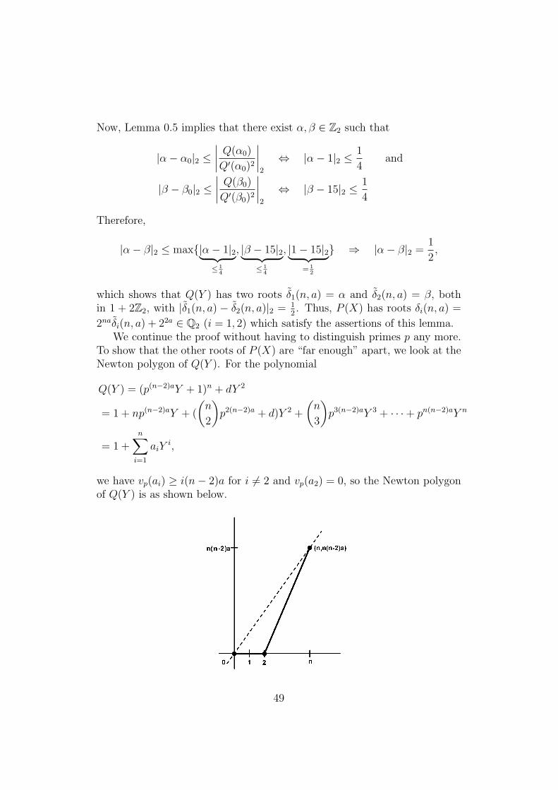
Now, Lemma 0.5 implies that there exist α, β ∈ Z2 such that

|α− α0|2 ≤∣∣∣∣ Q(α0)

Q′(α0)2

∣∣∣∣2

⇔ |α− 1|2 ≤1

4and

|β − β0|2 ≤∣∣∣∣ Q(β0)

Q′(β0)2

∣∣∣∣2

⇔ |β − 15|2 ≤1

4

Therefore,

|α− β|2 ≤ max{|α− 1|2︸ ︷︷ ︸≤ 1

4

, |β − 15|2︸ ︷︷ ︸≤ 1

4

, |1− 15|2︸ ︷︷ ︸= 1

2

} ⇒ |α− β|2 =1

2,

which shows that Q(Y ) has two roots δ1(n, a) = α and δ2(n, a) = β, bothin 1 + 2Z2, with |δ1(n, a) − δ2(n, a)|2 = 1

2. Thus, P (X) has roots δi(n, a) =

2naδi(n, a) + 22a ∈ Q2 (i = 1, 2) which satisfy the assertions of this lemma.We continue the proof without having to distinguish primes p any more.

To show that the other roots of P (X) are “far enough” apart, we look at theNewton polygon of Q(Y ). For the polynomial

Q(Y ) = (p(n−2)aY + 1)n + dY 2

= 1 + np(n−2)aY + (

(n

2

)p2(n−2)a + d)Y 2 +

(n

3

)p3(n−2)aY 3 + · · ·+ pn(n−2)aY n

= 1 +n∑i=1

aiYi,

we have vp(ai) ≥ i(n− 2)a for i 6= 2 and vp(a2) = 0, so the Newton polygonof Q(Y ) is as shown below.

49

Since there are two different slopes on it, λ = 0 of length 2 and λ = naof length n − 2, we conclude that there are two roots of Q(Y ) with p-adicabsolute value 1. These are exactly δ1(n, a) and δ2(n, a), while if δ is any ofthe other n− 2 roots, we have |δ|p = pna. Substituting back, we get that forevery root δ of P (X) different from δ1(n, a) and δ2(n, a) it holds

|δ|p = |pnaδ + p2a|p = 1 and likewise |δ − p2a|p = 1.

5.2 Main theorem and central part of its proof

Theorem 5.1 asserts the existence of p-adic numbers with special properties.

Theorem 5.1. Let n ≥ 3 be an integer and set F (n) = 2n3 + 2n2 + 3n. Letwn and w∗n be real numbers such that

w∗n ≤ wn ≤ w∗n +n

4, wn > F (n). (5.1)

Then there exist ξ ∈ Qp such that

w∗n(ξ) = w∗n and wn(ξ) = wn.

Proposition 5.1 below gives an explicit inductive construction of sequences(ξj)j≥1 of p-adic algebraic numbers of degree n. It will later be proved thatsuch carefully selected sequences converge to p-adic numbers having the prop-erties stated in Theorem 5.1. We use in the next proposition the same nota-tion as in Lemma 5.1, namely we denote by δ1(n, a) the root of the polynomialdefined in that lemma.

Proposition 5.1. Let n ≥ 3 be an integer and let µ, ν be real numbers with0 ≤ µ ≤ n/4 and ν > 1. Set H(n) = 2n3 + 2n2 + 2n + 1 and let χ > H(n)be a real number.

Then there exist a positive number λ < 1/2, an increasing sequence ofintegers g1 ≥ 5, g2, . . ., and a sequence of integers c1, c2, . . . such that thefollowing conditions are satisfied, where we have set γj := δ1(n, bµ logp gjc)for any integer j ≥ 1:(Ij) cj ∈ [gj/2, gj].(II1) ξ1 = −c1 + γ1.(IIj) ξj = −cj + γj belongs to the annulus Ij−1 ⊆ Qp defined by

1

2pg−νj−1 ≤ |x− ξj−1|p < g−νj−1.

50

(III1) |ξ1 − α|p ≥ 2λH(α)−χ for any algebraic number α 6= ξ1 of degree≤ n.(IIIj) |ξj − α|p ≥ λH(α)−χ for any algebraic number α 6∈ {ξ1, . . . , ξj} ofdegree ≤ n (j ≥ 2).

Proof. To simplify the notation, in what follows, we denote by α an algebraicnumber of degree ≤ n. Let ε be a positive number such that

χ > 2n3 + 2n2 + 2n+ 1 + 2n2ε. (5.2)

In order to prove this proposition, we add three extra conditions (IVj), (Vj)and (V Ij) which should be satisfied by the numbers ξj.

Set

Jj := {x ∈ Ij : |x− α|p ≥ 2λH(α)−χ for any algebraic α

of degree ≤ n, α 6= ξ1, . . . , ξj, x, H(α) ≥ (λgνj )1/χ}.

The extra conditions are:(IVj) ξj ∈ Jj−1 (j ≥ 2).

(Vj) H(α) ≤ g1/(n+1+ε)j ⇒ |ξj − α|p ≥ 1/gj (j ≥ 1).

(V Ij) µ(Jj) ≥ µ(Ij)/2 (j ≥ 1).Here as before, µ denotes the Haar measure.

We construct the numbers ξ1, ξ2, . . . by induction with description of stepsthe same as before (cf. [4, 7]). At the j-th stage, there are two steps. Step(Aj) consist in building an algebraic number

ξj = −cj + γj

satisfying conditions (Ij) to (Vj). In step (Bj), we show that the number ξjconstructed in (Aj) satisfies (V Ij) as well, provided that gj is chosen largeenough in terms of

n, µ, ν, χ, ε, λ, ξ1, . . . , ξj−1. (5.3)

The symbols o, � and � used throughout steps (Aj) and (Bj) mean thatthe numerical implicit constants depend (at most) on quantities (5.3). Fur-thermore, the symbol o implies ‘as gj tends to infinity’.

Note that we will have cj ∈ [gj/2, gj].Step (A1) is easy. There are � g1 possible numbers ξ1 = −c1 + γ1 and

since 0 < c1 ≤ g1, the distance between such numbers is

|(−c′1 + γ1)− (−c′′1 + γ1)|p = |c′1 − c′′1|p >1

g1

. (5.4)

51

There are only o(g1) algebraic numbers α of degree at most n satisfying

H(α) ≤ g1/(n+1+ε)1 , so we are able to choose ξ1 such that (V1) is satisfied.

Moreover, by Lemma 2.5, we have

|ξ1 − α|p ≥ 2λH(α)−n

with λ = c(n, n) H(ξ1)−n/2, for any algebraic number α 6= ξ1 of degree at

most n. Thus (I1), (II1), (III1) and (V1) are satisfied.Let j ≥ 2 be an integer and assume that ξ1, . . . , ξj−1 have been con-

structed. Step (Aj) is much harder to verify, since we have no control on theset Jj−1. Thus, it is difficult to check that the condition (IVj) holds, so weintroduce a new set J ′j−1 which contains Jj−1.

Set ξj = −cj + γj for some positive integers gj > gj−1 and cj ∈ [gj/2, gj]and denote by J ′j−1 the set of p-adic numbers x in Ij−1 satisfying |x −α|p ≥ 2λH(α)−χ for any algebraic number α of degree ≤ n, distinct fromξ1, . . . , ξj−1, x and whose height H(α) satisfies the inequalities

(λgνj−1)1/χ ≤ H(α) ≤

(c(n)−1g2n2

j )1/(χ−n), (5.5)

where c(n) is a constant depending only on n which will be defined in amoment. Since, by (5.2), we have

χ− n > 2n2(n+ 1), (5.6)

the exponent of gj in the right of (5.5) is strictly less than 1/(n+ 1). Thus,there are o(gj) algebraic numbers α satisfying (5.5). We will prove that forgj large enough we have� gj suitable choices for cj such that the conditions(Ij) to (IVj) are fulfilled.

Exactly the same argument as in the proof of Proposition 4.1 is applied toshow that µ(J ′j−1)� 1 (which is a consequence of J ′j−1 ⊃ Jj−1 and (V Ij−1))implies that there are � gj possible numbers ξj = −cj + γj ∈ J ′j−1. Thesenumbers trivially satisfy (IIj) and we will prove that they also satisfy (IVj)for gj large enough.

Let α be an algebraic number of degree ≤ n. We have

H(γj) = H(δ1(n, bµ logp gjc)

)= dp4bµ logp gjc ≤ dgnj

and Lemma 0.3 gives

H(ξj) = H(−cj + γj) ≤ 2n+1 H(γj) max{1, |cj|}n ≤ 2n+1 H(γj)gnj ≤ 2n+1dg2n

j .

We infer from Lemma 2.5 that there exist positive constants c(n) and c(n)such that

|ξj − α|p ≥ c(n) H(ξj)−n H(α)−n ≥ c(n)g−2n2

j H(α)−n. (5.7)

52

In particular, using 2λ < 1, we have

|ξj − α|p ≥ 2λH(α)−χ (5.8)

as soon asH(α)χ−n ≥ c(n)−1g2n2

j . (5.9)

This together with the definition of J ′j−1 shows that all our ξj ∈ J ′j−1 alsobelong to Jj−1. Therefore, the condition (IVj) is verified.

We are left with � gj suitable algebraic numbers ξj, mutually distant byat least g−1

j (compare with (5.4)). Only o(gj) algebraic numbers α of degreeat most n satisfy

H(α) ≤ g1/(n+1+ε)j , (5.10)

thus there are � gj algebraic numbers ξj such that |ξj − α|p ≥ 1/gj for thenumbers α verifying (5.10). Consequently, there are� gj algebraic numbersξj satisfying (Ij), (IIj), (IVj) and (Vj).

We still have to prove that such a ξj also satisfies (IIIj). To this end,because of (IVj), it suffices to show that

|ξj − α|p ≥ λH(α)−χ

holds for any algebraic number α of degree ≤ n, which is different fromξ1, . . . , ξj and whose height H(α) satisfies

H(α) < (λgνj−1)1/χ.

Since the sequence (gt)t≥1 is increasing, we either have

g−ν1 < λH(α)−χ, (5.11)

or there exists an integer t with 2 ≤ t < j such that

g−νt < λH(α)−χ ≤ g−νt−1. (5.12)

In the former case, we infer from (III1) and (5.11) that

|ξj − α|p ≥ |ξ1 − α|p − |ξj − ξ1|p ≥ 2λH(α)−χ − g−ν1 > λH(α)−χ.

In the latter case, (IVt) and (5.12) yield that

|ξj − α|p ≥ |ξt − α|p − |ξj − ξt|p ≥ 2λH(α)−χ − g−νt > λH(α)−χ.

Thus condition (IIIj) holds and the proof of step (Aj) is completed.

53

Before going on with the step (Bj), let us mention that the integer cj isfar from being uniquely determined. Indeed, at any step j we have � gjsuitable choices for ξj which shows that the construction actually gives anuncountable set of numbers.

Let j ≥ 1 be an integer. For the proof of step (Bj), we first establish thatif gj is large enough and if x lies in Ij, then we have

|x− α|p ≥ 2λH(α)−χ (5.13)

for any algebraic number α 6= ξj of degree ≤ n such that

(λgνj )1/χ ≤ H(α) ≤ gν/(χ−n−1−ε)j . (5.14)

Let, then, α 6= ξj be an algebraic number of degree ≤ n satisfying (5.14) andlet x be in Ij, that is, such that

1

2pg−νj ≤ |x− ξj|p < g−νj . (5.15)

If ν(n + 1 + εn) ≤ χ − n − 1 − ε, then H(α) ≤ g1/(n+1+ε)j and it follows

from (Vj), (5.14), (5.15) and the assumption ν > 1 that

|x− α|p ≥ |ξj − α|p − |ξj − x|p ≥ g−1j − g−νj ≥ 2g−νj ≥ 2λH(α)−χ, (5.16)

provided that gj is large enough.Otherwise, we have

ν(n+ 1 + ε) > χ− n− 1− ε, (5.17)

and, by (5.7), we get

|x− α|p ≥ |ξj − α|p − |ξj − x|p≥ c(n)g−2n2

j H(α)−n − g−νj≥ c(n)g−2n2

j H(α)−n/2.

(5.18)

The last inequality holds if

2g−νj ≤ c(n)g−2n2

j H(α)−n. (5.19)

In view of (5.14), inequality (5.19) is true as soon as

2gnν/(χ−n−1−ε)j ≤ c(n)gνj g

−2n2

j ,

54

which, by (5.17), holds for gj large enough when

n

χ− n− 1− ε< 1− 2n2 n+ 1 + ε

χ− n− 1− ε, (5.20)

and in particular when χ satisfies (5.2). Furthermore, we have

c(n)g−2n2

j H(α)−n ≥ 4λH(α)−χ. (5.21)

Indeed, by (5.14), λ < 1, and (5.17), we get

H(α)χ−n ≥ (λgνj )(χ−n)/χ ≥ λg(χ−n)(χ−n−1−ε)/(χn+χ+χε)j

≥ 4λc(n)−1g2n2

j ,

since we infer from (5.2) that

(χ− n)(χ− n− 1− ε) > 2χn2(n+ 1 + ε). (5.22)

Combining (5.18) and (5.21), we have verified that

|x− α|p ≥ 2λH(α)−χ

holds under assumption (5.17). By (5.16), this implies that (5.13) is true ifα satisfies (5.14) and is not equal to ξj. Consequently, for gj large enough,the complement J cj of Jj in Ij is contained in the union of the balls

B(α, 2λH(α)−χ),

where α ∈ Qp runs over the algebraic numbers of degree ≤ n and height

greater than gν/(χ−n−1−ε)j . The Haar measure of J cj is then

�∑

H>gν/(χ−n−1−ε)j

Hn−χ = o(g−νj ) = o(µ(Ij)).

Thus, we conclude that we can find gj large enough such that µ(Jj) ≥µ(Ij)/2. This completes step (Bj) as well as proof of Proposition 5.1.

At this moment, we can recap where the condition χ > 2n3 +2n2 +2n+1was used. There are three steps where it was needed, namely (5.6), (5.20)and (5.22). Asymptotically, these three inequalities reduce, respectively, toχ− n > 2n2(n + 1), χ− n− 1 > 2n2(n + 1) + n, and (χ− n)(χ− n− 1) >2χn2(n + 1). The most restricting condition is given by (5.20), hence, ourassumption on χ.

55

5.3 Proof of Theorem 5.1

Let wn and w∗n be two real numbers fulfilling the conditions of Theorem5.1. We will define numbers which are needed to apply Proposition 5.1. Setµ = wn − w∗n ∈ [0, n/4], ν = n(w∗n + 1) and finally, set χ = wn − n + 1, sothat χ > H(n) = 2n3 + 2n2 + 2n+ 1.

Let λ and ξ1, ξ2, . . . be as in Proposition 5.1 and denote by ξ ∈ Qp thelimit of the Cauchy sequence (ξj)j≥1.

The constants implied in � and � of this section depend at most on pand n. Our choice of γj implies that the minimal polynomial of ξj over Z is

Qj(X) := (X + cj)n + d

((X + cj)− p2bµ logp gjc

)2.

This polynomial is indeed primitive and irreducible by the first statement ofLemma 5.1.

Since cj ∈ [gj/2, gj] and µ ≤ n/4, we have H(ξj) = H(Qj) � gnj . More-over, for any j ≥ 1

|ξ − ξj|p ∈ [1

2pg−νj , g−νj [

and we deduce that

|ξ − ξj|p � H(ξj)−ν/n � H(ξj)

−w∗n−1. (5.23)

Further, if α is of degree ≤ n and is not one of the ξj’s, then |ξ − α|p ≥λH(α)−χ, whence

|ξ − α|p ≥ H(α)−w∗n−1 (5.24)

since χ ≤ w∗n + 1. It follows from (5.23), (5.24) and our remarks on thedefinition of w∗n(ξ) from §4.1 that w∗n(ξ) = w∗n.

It now remains to prove that wn(ξ) = wn. Denote by ξj = βj1, . . . , βjnthe roots of Qj(X), numbered in such a way that βj2 is closest to ξj. Denoteby δ3, . . . , δk the roots of Pn,bµ logp gjc(X) other than δi(n, bµ logp gjc), i = 1, 2.Then using Lemma 5.1, we get

|ξj − βj2|p = |(−cj + γj)− (−cj + δ2(n, bµ logp gjc))|p= |δ1(n, bµ logp gjc)− δ2(n, bµ logp gjc)|p= p−nbµ logp gjc � g−nµj

and|ξj − βjk|p = |γj − δk|p = 1, for k ≥ 3.

56

Keeping in mind that |ξ − βj2|p = |ξj − βj2|p since |ξj − βj2|p > |ξ − ξj|p, wearrive at

|Qj(ξ)|p = |ξ − ξj|p|ξ − βj2|p∏

3≤k≤n

|ξ − βjk|p

� H(ξj)−w∗n−1g−nµj

� H(Qj)−w∗n−µ−1.

We see thatwn(ξ) ≥ w∗n + µ. (5.25)

Now we will show that (5.25) is indeed an equality. Let P (X) be aninteger polynomial of degree ≤ n which is not a multiple of some Qj(X).Write

P (X) = aR1(X) · · ·Rs(X),

where a is an integer and the polynomialsRi(X) are primitive and irreducible.Since Ri(ξ) 6= 0, if k denotes the degree of the polynomial Ri(X), then byLemma 2.4, this polynomial has a root θ satisfying

|Ri(ξ)|p � H(Ri)1−k|ξ − θ|p � λH(Ri)

−χ−k+1 � λH(Ri)−wn . (5.26)

Consequently, it follows from (5.26) and Gelfond’s Lemma 0.2 that

|P (ξ)|p �(

H(R1) · · ·H(Rs))−wn � H(P )−wn

and we get wn(ξ) = wn as claimed.

5.4 The case n = 1

Solely for completeness, we include the following proposition which dealswith the case n = 1.

Proposition 5.2. For every ξ ∈ Qp \Q we have w1(ξ) = w∗1(ξ) ≥ 1. More-over, for every w ∈ [1,+∞], there are uncountably many ξ ∈ Qp such thatw1(ξ) = w∗1(ξ) = w.

Proof. The lower bound w1(ξ) ≥ 1 follows from the general case proved byMahler [21] and is basically a consequence of Dirichlet’s pigeonhole principle.

The equality w1(ξ) = w∗1(ξ) is obtained from the inequality w1(ξ) ≥w∗1(ξ), which is trivial in this case, and the reversed inequality, which becomesobvious if we notice that for a reduced fraction a/b ∈ Q such that |ξ−a/b|p <|ξ|p, we have |a/b|p = |ξ|p and therefore min{|a|p, |b|p} ≥ min{|ξ|p, 1/|ξ|p}.

The second part of this proposition is deduced for example during com-putation of Hausdorff dimension of sets {ξ ∈ Qp : wn(ξ) = w}, w ≥ n, see[7, Theorem 9.6] or [2, §6].

57

If w > 1+√

52

, we can give a simple construction of ξ ∈ Qp such thatw∗1(ξ) = w.

Proposition 5.3. Let w > 1+√

52

and

ξ =∞∑i=1

aipb(w+1)ic ∈ Qp,

where ai ∈ {1, . . . , p− 1} for all i ≥ 1. Then w1(ξ) = w∗1(ξ) = w.

Proof. Take any w > 1+√

52

and let ξk =∑k

i=1 aipb(w+1)ic. All the implicit

constants in � and � in this proof depend at most on p. Since

|ξ − ξk|p = p−b(w+1)k+1c � ξ−w−1k

for any k ≥ 1, we have w∗1(ξ) ≥ w.For a reduced fraction a/b ∈ Q whose height is large enough, let l ≥ 1 be

such thatξl ≤ H(a/b) < ξl+1.

Suppose that ∣∣∣ξ − a

b

∣∣∣p

= H(ab

)−ν,

where ν > w + 1. We have

|ξ − ξl|p = |ξl+1 − ξl|p = p−b(w+1)l+1c � ξ−w−1l ,

|ξ − ξl+1|p = p−b(w+1)l+2c � ξ−w−1l+1 � ξ

−(w+1)2

l .

Therefore,

1

|b|ξl + |a|≤∣∣∣bξl − a

b

∣∣∣p

=∣∣∣ξl − a

b

∣∣∣p≤ max{|ξ − ξl|p,

∣∣∣ξ − a

b

∣∣∣p} (5.27)

� max{ξ−w−1l ,H(a/b)−ν} = ξ−w−1

l and

1

|b|ξl+1 + |a|≤∣∣∣ξl+1 −

a

b

∣∣∣p≤ max{|ξ − ξl+1|p,

∣∣∣ξ − a

b

∣∣∣p} (5.28)

� max{ξ−w−1l+1 ,H(a/b)−ν}.

From (5.27) we get

ξw+1l � |b|ξl + |a| � H(a/b)(ξl + 1)� H(a/b)ξl, i.e.

ξwl � H(a/b). (5.29)

58

From (5.28) we get

min{ξw+1l+1 ,H(a/b)ν} � |b|ξl+1 + |a| � H(a/b)ξl+1.

Since ξwl+1 � H(a/b) does not hold, we must have

H(a/b)ν � H(a/b)ξl+1, i.e.

H(a/b)� ξ1

ν−1

l+1 � ξ1wl+1 � ξ

w+1w

l . (5.30)

If there is an infinite sequence akbk∈ Q such that

lim supk→∞

− log |ξ − akbk|p

log H(ak/bk)> w,

then H(ak/bk) → ∞ when k → ∞ and we conclude from (5.29) and (5.30)

that w ≤ w+1w

which implies w ≤ 1+√

52

, contrary to our choice of w.Hence, it must hold that w∗1(ξ) = w.

5.5 On w2 − w∗2Lemma 5.2. There exists a family of irreducible integer polynomials

Pm(X) = X2 + amX + bm, m ≥ 1

with roots in Qp such that am + 1 ≥ |bm|, am � pm and

sepp(Pm) � H(Pm)−1,

where the implicit constants depend only on p.

Proof. We first examine the case p 6= 2. Let g be the smallest prime suchthat g ≡ 1 (mod 4p). Its existence is guaranteed by Dirichlet’s theorem onprimes in arithmetic progressions.

Let

lm =⌊pm√g

2+

1

2

⌋.

Then it is easy to see that

(2lm − 1)2 ≤ p2mg < (2lm + 1)2

and we put am = 2lm − 1 if p2mg ≤ 12

((2lm − 1)2 + (2lm + 1)2

)= 4l2m + 1.

Otherwise, we put am = 2lm + 1. Since (2lm + 1)2 − (2lm − 1)2 = 8lm, if we

59

now set bm = 14(a2m − p2mg), it must be |bm| ≤ 1

48lm = 2lm ≤ am + 1, while

bm ∈ Z is assured by a2m ≡ (2lm ± 1)2 ≡ 1 (mod 4) and p2mg ≡ (±1)2m1 ≡ 1

(mod 4).Hensel’s Lemma 0.5 ensures that the polynomial Q(X) = X2 − g has

roots δ ∈ 1 + pZp and −δ ∈ −1 + pZp. Thus the polynomial

Pm(X) = X2 + amX + bm =1

4

((2X + am)2 − p2mg

)=p2m

4Q(2X + am

pm

)has roots −am±p

mδ2

, which are in Qp and their distance is

sepp(Pm) = |pmδ|p = p−m � a−1m � H(Pm)−1.

If p = 2, we take lm = b2m√

17c, and put either am = 2lm or am = 2lm+2

depending for which choice a2m is closer to 22(m+1)17. Taking b2m = a2

m

4−22m17,

it can easily be checked that all the claims of this lemma are fulfilled.

We will prove the next theorem which is analogous to a result for the realnumbers from [6].

Theorem 5.2. The set of values taken by the function w2−w∗2 contains theinterval [0, 1[.

In view of (4.1), Theorem 5.2 is essentially best possible. Unfortunately,our method of proof does not enable us to deduce whether there exist ξ ∈ Qp

such that w2(ξ) = w∗2(ξ) + 1.The proof of Theorem 5.2 basically follows that of Theorems 4.1 and 5.1.

The key point is the existence of a family of quadratic integer polynomialsfrom Lemma 5.2 having two p-adic roots very close to each other. We willnot give a full proof of this theorem, but merely explain which lines from theProposition 5.1, Theorem 5.1 and their proofs need to be modified beyondthe simple substitution n = 2.

Proposition 5.4. Let µ, ν, χ be real numbers such that µ ∈]1/2, 1[, ν > 1and χ is sufficiently large with respect to µ, for example χ > 12(2 + µ

1−µ).

Then there exist a positive number λ < 1/2, an increasing sequence ofintegers g1, g2, . . ., and a sequence of integers c1, c2, . . . such that the followingconditions are satisfied for any integer j ≥ 1:(Ij) cj ∈ [gj/2, gj] and γj is one root of polynomial Pmj(X) = X2 +amjX+

bmj from Lemma 5.2 where mj is such that amj � gµ

1−µj .

(II1) ξ1 = −c1 + γ1.(IIj) ξj = −cj + γj belongs to the annulus Ij−1 ⊆ Qp defined by

1

2pg−νj−1 ≤ |x− ξj−1|p < g−νj−1.

60

(III1) |ξ1 − α|p ≥ 2λH(α)−χ for any algebraic number α 6= ξ1 of degree≤ 2.(IIIj) |ξj − α|p ≥ λH(α)−χ for any algebraic number α 6∈ {ξ1, . . . , ξj} ofdegree ≤ 2 (j ≥ 2).

Proof (sketch). For ease of writing, denote τ = 2 + µ1−µ . The main difference

from the proof of Proposition 5.1 is that inequalities (5.9) no longer hold.Therefore, we need to make the following modifications:

(λgνj−1)1/χ ≤ H(α) ≤

(c(µ)−1g2τ

j )1/(χ−2) (5.5’)

χ− 2 > 6τ (5.6’)

H(ξj) ≤ 8 H(γj)g2j < c(µ)gτj

|ξj − α|p ≥ cH(ξj)−2 H(α)−2 ≥ c(µ)g−2τ

j H(α)−2 (5.7’)

H(α)χ−2 ≥ c(µ)−1g2τj (5.9’)

|x− α|p ≥ c(µ)g−2τj H(α)−2/2 (5.18’)

2g−νj ≤ c(µ)g−2τj H(α)−2 (5.19’)

2

χ− 3− ε< 1− 2τ

3 + ε

χ− 3− ε(5.20’)

c(µ)g−2τj H(α)−2 ≥ 4λH(α)−χ (5.21’)

(χ− 2)(χ− 3− ε) > 2τχ(3 + ε) (5.22’)

We see that for example χ > 12τ = 12(2 + µ1−µ) satisfies all the conditions

(5.6’) (5.20’), (5.22’) for ε small enough, say 0 < ε < 1.

Proof of Theorem 5.2 (sketch). The function w2−w∗2 certainly takes all val-ues from [0, 1/2] according to Theorem 4.1, so we are only concerned withthe interval ]1/2, 1[. Pick µ from that interval, χ large enough, w2 ≥ χ + 1,w∗2 = w2 − µ and ν = 1

1−µ(w∗2 + 1). Apply Proposition 5.4 and set ξ =limj→∞ ξj ∈ Qp.

The minimal polynomial of ξj over Z is

Qj(X) := Pmj(X + cj) = (X + cj)2 + amj(X + cj) + bmj .

Noting that we employ the usual notation for algebraic conjugates and thatthe implicit constants in � depend only on p and µ, it holds

H(ξj) = H(Qj) � cj max{amj , cj} � cjamj � g1

1−µj

61

since amj � gµ

1−µj , cj � gj and µ ∈]1/2, 1[. Also,

|ξ − ξj|p � g−νj � H(ξj)−w∗2−1,

|ξ − ξ′j|p = |ξj − ξ′j|p = |γj − γ′j|p = sepp(Pmj) � a−1mj,

|Qj(ξ)|p = |ξ − ξj|p|ξ − ξ′j|p � H(ξj)−w∗2−1a−1

mj� H(Qj)

−w∗2−µ−1.

Therefore, w2(ξ) ≥ w∗2 + µ = w2 and the rest of the proof, just like all thedetails, is the same as the proof of Theorem 5.1.

62

Chapter 6

Some results on w∗n

Mahler proved in [20] that his classification of real numbers has the propertythat every two algebraically dependent numbers belong to the same class. Inorder to prove this basic property he showed that if ξ and η are transcendentalreal numbers such that P (ξ, η) = 0 for an irreducible polynomial P (x, y) ∈Z[x, y] of degree M in x and N in y, then the inequalities

wn(ξ) + 1 ≤M(wnN(η) + 1) and wn(η) + 1 ≤ N(wnM(ξ) + 1) (6.1)

are valid for every positive integer n. Schmidt [29, (4), p. 276] showed thatthese conditions also imply inequalities

w∗n(ξ) + 1 ≤M(w∗nN(η) + 1) and w∗n(η) + 1 ≤ N(w∗nM(ξ) + 1), (6.2)

i.e. the analogous inequalities we get when Mahler’s function wk is replacedwith Koksma’s function w∗k.

Mahler himself [21] proved the inequalities (6.1) under analogous condi-tions in the p-adic setting. We will establish in this chapter a p-adic versionof (6.2). Let us mention that our proof is in different fashion from whatMahler did in [21] and is more in vein with [29].

Our first lemma is valid for every algebraic number, whether we take itfrom C or Cp.

Lemma 6.1. Let α be an algebraic number of degree n and let

P (x) = anxn + · · ·+ a0 = an(x− α)(x− α2) · · · (x− αn)

be its minimal polynomial over Z. Then if k1, . . . , kt are distinct numbersamong 1, . . . , n, the number anαk1 · · ·αkt is an algebraic integer.

Proof. See [31, Hilfssatz 17, p. 77].

63

The second lemma deals with the standard representation of symmetricpolynomials through elementary symmetric polynomials but with an impor-tant observation that will later be required.

Lemma 6.2. Let P (t1, . . . , tk) ∈ Z[t1, . . . , tk] be a homogeneous symmetricpolynomial. Denote

degt1 P = · · · = degtk P = d.

There exists a unique polynomial Q(x1, . . . , xn) ∈ Z[x1, . . . , xn] such that

P (t1, . . . , tk) = Q(s1, . . . , sk),

where si = si(t1, . . . , tk) (1 ≤ i ≤ k) are elementary symmetric polynomialsof t1, . . . , tk. For every monomial si11 · · · s

ikk in Q(s1, . . . , sk), we have i1 +

· · ·+ ik ≤ d.

Proof. See [19, Theorem 6.1, §IV.6, p. 191], [14, Theorem 3.3.1, p. 25], [11,Exercise 13, §7.1, p. 326].

Now we prove the announced result.

Theorem 6.1. Let ξ, η ∈ Qp be two transcendental numbers which are al-gebraically dependent. Suppose P (x, y) ∈ Z[x, y] is a non-zero polynomialirreducible over Q, of degree M in x and degree N in y such that P (ξ, η) = 0.Then for every positive integer n, it holds

w∗n(ξ) + 1 ≤M(w∗nN(η) + 1) and w∗n(η) + 1 ≤ N(w∗nM(ξ) + 1).

Proof. Of course, it is enough to prove only the first inequality since thesecond follows by interchanging ξ and η.

Fix a positive integer n. It is not hard to see from Lemma 0.3 that forany integer l 6= 0 we have w∗n(ξ) = w∗n(lξ) and w∗n(η) = w∗n(lη). Hence, bytaking l to be a large power of p and multiplying the polynomial P (x, y) bythe appropriate power of p, we see that without loss of generality we cansuppose ξ, η ∈ Zp.

The partial derivatives of P (x, y) do not vanish at (ξ, η). Suppose to thecontrary that ∂

∂yP (x, y) vanishes at (ξ, η). By considering P (ξ, y) as a poly-

nomial in y with coefficients in Q(ξ), one sees that P (ξ, y) = P ∗1 (ξ, y)P ∗2 (ξ, y),where P ∗1 (ξ, y), P ∗2 (ξ, y) are polynomials of positive degree in y, with coeffi-cients in Q(ξ). Since ξ is transcendental, Q(ξ) is isomorphic to Q(x), so infact we have P (x, y) = P ∗1 (x, y)P ∗2 (x, y), where P ∗1 (x, y), P ∗2 (x, y) ∈ Q(x)[y].But Q(x) is the fraction field of Q[x], so by Gauss’s Lemma 0.1 we can

64

find polynomials P1(x, y), P2(x, y) ∈ Q[x, y] of positive degree in y and withP (x, y) = P1(x, y)P2(x, y). This contradicts the irreducibility of P (x, y).

Let H > 1 and suppose β ∈ Qp is an algebraic number with deg(β) ≤ n,H(β) ≤ H such that w∗n(ξ,H) = |ξ − β|p. Obviously, if H is large enough,w∗n(ξ,H) becomes as small as we want, and since ξ ∈ Zp, we can assumeβ ∈ Zp as well. Since P (x, y) and ∂

∂yP (x, y) are polynomials, there exist ε,

c1, c2 all positive real numbers depending only on P (x, y) (in other words,only on ξ and η) such that for any u ∈ Qp

|u− ξ|p < ε ⇒

|P (u, η)|p = |P (u, η)− P (ξ, η)|p < c1|u− ξ|p,∣∣∣∣ ∂∂yP (u, η)− ∂

∂yP (ξ, η)

∣∣∣∣p

<1

2

∣∣∣∣ ∂∂yP (ξ, η)

∣∣∣∣p

= c2 > 0.

If we take H large enough, we get

|ξ − β|p < min{ε,c222c1

},

which implies

|P (β, η)|p < c1|β − ξ|p <c222

and

∣∣∣∣ ∂∂yP (β, η)

∣∣∣∣p

> c2.

Therefore, ∣∣∣∣∣ P (β, η)(∂∂yP (β, η)

)2∣∣∣∣∣p

<1

2

and if we look at P (β, y) as a polynomial in y, we see that the conditionsof Lemma 0.5 are fulfilled. This lemma implies there is a β′ ∈ Zp such thatP (β, β′) = 0 and

|β′ − η|p ≤

∣∣∣∣∣ P (β, η)(∂∂yP (β, η)

)2∣∣∣∣∣p

<c1c22|β − ξ|p � |β − ξ|p = w∗n(ξ,H),

where the implied constants in � and � everywhere they appear in thisproof depend at most on ξ, η and n.

Let Q(x) = ak(x − β1) · · · (x − βk) (k ≤ n) be the minimal polynomialof β = β1 over Z. The number β′ is a root of the polynomial P (β, y) in y,hence a root of the polynomial

R(y) = aMk P (β1, y)P (β2, y) · · ·P (βk, y).

65

The polynomial P (β, y) is not identically zero, since P (x, y) would otherwisebe divisible by the minimal polynomial of β. Thus R(y) is not identicallyzero. The coefficients of R(y) are linear combinations with rational integercoefficients of terms of the type

aMk∑σ

βi1σ(1) · · · βikσ(k),

where the sum is taken over all permutations σ of {1, . . . , k} while 0 ≤ ij ≤M for 1 ≤ j ≤ k. But, because of Lemma 6.2 and Viete’s formulas forthe polynomial Q(x), such terms are rational integers themselves and �H(Q)M ≤ HM . Therefore, R(y) ∈ Z[y] and H(R) � HM . Since R(β′) = 0,we see that β′ is algebraic and its minimal polynomial over Z is a factor ofR(y). Using Gauss’s Lemma 0.1 and Gelfond’s Lemma 0.2, we get that thisminimal polynomial also has coefficients � HM . Hence H(β′) � HM , sayH(β′) ≤ cHM . Thus

w∗nN(η, cHM) ≤ w∗kN(η, cHM) ≤ |η − β′|p � w∗n(ξ,H)⇒

w∗nN(ξ) + 1 = lim supH→∞

− log(w∗nN(ξ, cHM))

log(cHM)

≥ 1

Mlim supH→∞

− log(w∗n(ξ,H))

logH=

1

M(w∗n(ξ) + 1).

We are able to show that the inequalities in (6.2) are sharp at least in avery special situation.

Proposition 6.1. Let k ≥ 1 be an integer, w be a real number such that

w > −1 + k +k2 + k

√k2 + 4k

2

and

ξ = a0 +∞∑i=1

aipb(w+1)ic ∈ Qp,

where ai ∈ {1, . . . , p−1} for all i ≥ 0. Then w∗1(ξ) = w and w∗1(ξk) = w+1k−1.

Proof. It has been shown in Proposition 5.3 that w∗1(ξ) = w. We claim thatw∗1(ξk) = w+1

k− 1 and, thus,

w∗1(ξ) + 1 = k(w∗1(ξk) + 1

),

66

so that inequality (6.2.i) becomes an equality for this special choice of η = ξk

and n = 1.Using similar notation as in Proposition 5.3, we have

|ξk − ξkl |p = |(ξl + ρlpb(w+1)l+1c)k − ξkl |p

� p−b(w+1)l+1c

� ξ−(w+1)l � (ξkl )−

w+1k ,

with ρl being some element in Zp \ pZp and constants in � depending onlyon p and k. Hence,

w∗1(ξk) ≥ w + 1

k− 1.

In order to show that the last inequality is actually an equality, we proceedjust like in the proof of Proposition 5.3. Let a/b ∈ Q be a reduced fractionsuch that

ξkl ≤ H(a/b) < ξkl+1

and ∣∣∣ξ − a

b

∣∣∣p

= H(ab

)−ν,

where ν > w+1k

.Instead of (5.29), we now have

(ξkl )w+1k−1 ≤ H(a/b)

and instead of (5.30),

H(a/b) ≤ (ξkl )k(w+1)w+1−k

where we used the fact that w + 1 > 2k which obviously holds if w satisfiesthe conditions of this proposition.

If we had w∗1(ξk) > w+1k− 1, we could conclude that

w + 1

k− 1 ≤ k(w + 1)

w + 1− kwhich contradicts the lower bound on w imposed in the statement of thisproposition.

Remark 6.1. Set

ξ = a0 +∞∑i=1

ai10−b(w+1)ic ∈ R,

where ai ∈ {1, 2, . . . , 9} for all i ≥ 0 and the same condition on w as in Propo-sition 6.1. Proceeding completely analogously as in the proof of Proposition6.1, we get a new example in the real numbers for which equality in (6.2.i)holds. See also [7, §3.7,§7.7].

67

Bibliography

[1] R. C. Baker, On approximation with algebraic numbers of bounded de-gree, Mathematika 23 (1976), no. 1, 18–31.

[2] V. I. Bernik and M. M. Dodson, Metric Diophantine approximation onmanifolds. Cambridge Tracts in Mathematics, 137. Cambridge Univer-sity Press, Cambridge, 1999.

[3] E. Bombieri and W. Gubler, Heights in Diophantine geometry. NewMathematical Monographs, 4. Cambridge University Press, Cambridge,2006.

[4] Y. Bugeaud, Mahler’s classification of numbers compared withKoksma’s, Acta Arith. 110 (2003), 89–105.

[5] Y. Bugeaud, Mahler’s classification of numbers compared withKoksma’s, II, In: Diophantine approximation. Festschrift for WolfgangSchmidt. Ed. H.-P. Schlickewei, K. Schmidt and R. F. Tichy, Develop-ments in Mathematics 16, pp. 107–121 (2008), Springer Wien.

[6] Y. Bugeaud, Mahler’s classification of numbers compared withKoksma’s, III, Publ. Math. Debrecen 65 (2004), 305–316.

[7] Y. Bugeaud, Approximation by algebraic numbers. Cambridge Tractsin Mathematics, Cambridge, 2004.

[8] Y. Bugeaud and A. Dujella, Root separation for irreducible integer poly-nomials, Bull. Lond. Math. Soc., to appear.

[9] Y. Bugeaud and M. Mignotte, Polynomial root separation, Intern. J.Number Theory 6 (2010), 587–602.

[10] J. W. S. Cassels, Local fields. London Mathematical Society StudentTexts, 3. Cambridge University Press, Cambridge, 1986.

68

[11] D. Cox, J. Little, and D. O’Shea, Ideals, varieties, and algorithms. Anintroduction to computational algebraic geometry and commutative al-gebra. Third edition. Undergraduate Texts in Mathematics. Springer,New York, 2007.

[12] K. Dorge, Uber die Seltenheit der reduziblen Polynome und der Normal-gleichungen, Math. Ann. 95 (1926), no. 1, 247256.

[13] A. Dujella and T. Pejkovic, Root separation for reducible monic quartics,Rend. Semin. Mat. Univ. Padova, to appear.

[14] J.-P. Escofier, Theorie de Galois. Cours avec exercices corriges. Enseigne-ment des Mathematiques. Masson, Paris, 1997.

[15] J.-H. Evertse, Distances between the conjugates of an algebraic number,Publ. Math. Debrecen 65 (2004), 323–340.

[16] F. Q. Gouvea, p-adic numbers. An introduction. Second edition. Uni-versitext. Springer-Verlag, Berlin, 1997.

[17] N. Koblitz, p-adic numbers, p-adic analysis, and zeta-functions. Secondedition. Graduate Texts in Mathematics, 58. Springer-Verlag, New York,1984.

[18] J. F. Koksma, Uber die Mahlersche Klasseneinteilung der transzenden-ten Zahlen und die Approximation komplexer Zahlen durch algebraischeZahlen, Monatsh. Math. Phys. 48, (1939), 176–189.

[19] S. Lang, Algebra. Revised third edition. Graduate Texts in Mathematics,211. Springer-Verlag, New York, 2002.

[20] K. Mahler, Zur Approximation der Exponentialfunktion und des Loga-rithmus. I, II, J. Reine Angew. Math. 166 (1932), 118–150.

[21] K. Mahler, Uber eine Klassen-Einteilung der p-adischen Zahlen, Math-ematica Leiden 3 (1935), 177–185.

[22] K. Mahler, An inequality for the discriminant of a polynomial, MichiganMath. J. 11 (1964), 257–262.

[23] M. Mignotte, Mathematics for computer algebra. Springer-Verlag, NewYork, 1992.

[24] J. F. Morrison, Approximation of p-adic numbers by algebraic numbersof bounded degree, J. Number Theory 10 (1978), no. 3, 334–350.

69

[25] H. Osada, The Galois groups of the polynomials Xn+aX l+b, J. NumberTheory 25 (1987), no. 2, 230–238.

[26] T. Pejkovic, On p-adic T -numbers, preprint.

[27] V. V. Prasolov, Polynomials. Algorithms and Computation in Mathe-matics, 11. Springer-Verlag, Berlin, 2004.

[28] H. P. Schlickewei, p-adic T -numbers do exist, Acta Arith. 39 (1981), no.2, 181–191.

[29] W. M. Schmidt, Mahler’s T -numbers, 1969 Number Theory Institute(Proc. Sympos. Pure Math., Vol. XX, State Univ. New York, StonyBrook, N.Y., 1969), pp. 275–286. Amer. Math. Soc., Providence, R.I.,1971.

[30] W. M. Schmidt, Diophantine Approximations and Diophantine Equa-tions. Lecture Notes in Math. 1467, Springer, Berlin, 1991.

[31] T. Schneider, Einfuhrung in die transzendenten Zahlen. Springer-Verlag,Berlin-Gottingen-Heidelberg, 1957.

[32] A. Schonhage, Polynomial root separation examples, J. Symbolic Com-put. 41 (2006), 1080–1090.

[33] Th. Skolem, Untersuchungen uber die moglichen Verteilungen ganz-zahliger Losungen gewisser Gleichungen, Videnskapsselskapets Skr. I(1921), Nr. 17, 57 S.

[34] U. Zannier, On the Hilbert irreducibility theorem, Rend. Semin. Mat.Univ. Politec. Torino 67 (2009), no. 1, 1–14.

70

Acknowledgements

I was a member of the European Doctoral College of the University of Stras-bourg during the preparation of my PhD, from 2007 to 2011, class nameMarco Polo. I have benefited from specific financial supports offered by theCollege and, along with my mainstream research, have followed a specialcourse on topics of general European interests presented by international ex-perts. This PhD research project has been led with the collaboration of twouniversities: University of Zagreb, Croatia and the University of Strasbourg,France.

I am grateful to my supervisors, professor Yann Bugeaud at the Universityof Strasbourg and professor Andrej Dujella at the University of Zagreb, fortheir commitment and direction of my research.

I wish to thank my parents Radoslav and Ana, and my brothers Branimirand Marko, for their love and support. I also thank my aunt Ruza for herencouragement.

71

Summary

Polynomial root separation and applicationsIn this thesis we study bounds on the distances of roots of integer poly-

nomials and applications of such results. Denote by sep(P ) the minimaldistance of roots of the separable integer polynomial P (X) and by H(P )maximum of the absolute values of its coefficients.

In the first chapter which looks at polynomial roots in the set of complexnumbers, we first summarize results on quadratic and cubic polynomials.The bulk of this chapter is dedicated to quartic polynomials and especiallyreducible monic integer polynomials of fourth degree. We show that forsuch polynomials sep(P ) � H(P )−2 but also construct families (Pk(X)) ofsuch polynomials that have sep(P ) � H(P )−2. The case when coefficients ofPk(X) are polynomials in k is studied more thoroughly.

In the second chapter different lemmas on roots of polynomials in thep-adic setting are proved. These lemmas are mostly analogues of the resultsin the real and complex case and are used later in the thesis.

In the third chapter explicit families of polynomials of general degree nare given which bound the exponent above H(P ) from the other side thansepp(P ) � H(P )−n+1. Results are proved using Newton polygons. Thenthe case of quadratic and reducible cubic polynomials in the p-adic settingis completely solved which shows that the bound above is really attained inthose classes of polynomials. For irreducible cubic polynomials a bound witha new, better exponent is exhibited.

The rest of the thesis is concerned with results on p-adic versions ofMahler’s and Koksma’s functions wn and w∗n and the related classificationsof transcendental numbers in Cp.

In the fourth chapter the main result is a construction of numbers suchthat the two functions wn and w∗n differ on them for every n. We can evenrequire wn − w∗n to be a chosen number in some small interval. The proof isquite involved and follows R. C. Baker’s proof in the real case.

In the fifth chapter the interval of possible values for wn−w∗n is expandedusing an effective estimate for the distance of algebraic numbers and a familyof polynomials with very close roots. The main proof in this chapter followsthe one in the previous chapter, but is a little easier since we restrict ourselvesto one or finitely many n. Special attention is given to cases n = 1 and n = 2.

In the last chapter inequalities linking values of Koksma’s functions foralgebraically dependent numbers are proved.

72

Resume

Separation des racines des polynomes et applicationsDans cette these, nous etudions les bornes sur les distances des racines

des polynomes entiers et les applications de ces resultats. Notons par sep(P )la distance minimale des racines du polynome entier separable P (X) et parH(P ) le maximum des valeurs absolues de ses coefficients.

Dans le premier chapitre, qui examine les racines des polynomes dansl’ensemble des nombres complexes, nous avons d’abord resume les resultatssur les polynomes quadratiques et cubiques. L’essentiel de ce chapitre estconsacre aux polynomes quartiques et surtout aux polynomes reductiblesnormalises de quatrieme degre a coefficients entiers. Nous avons montre quepour de tels polynomes sep(P ) � H(P )−2, mais aussi construit des familles(Pk(X)) de tels polynomes qui ont sep(P ) � H(P )−2. Le cas ou les coefficientsde Pk(X) sont polynomes en k est etudie plus a fond.

Dans le deuxieme chapitre differents lemmes sur les racines des polynomesen nombres p-adiques sont prouves. Ces lemmes sont pour la plupart ana-logues aux resultats dans le cas reel et complexe et sont utilises plus tarddans la these.

Dans le troisieme chapitre sont donnees les familles explicites de po-lynomes de degre n qui bornent l’exposant de H(P ) de l’autre cote quesepp(P ) � H(P )−n+1. Les resultats sont prouves en utilisant des polygonesde Newton. Ensuite, le cas des polynomes quadratiques et des polynomes cu-biques reductibles dans les p-adiques est resolu completement, ce qui montreque la limite presentee ci-dessus est vraiment atteinte dans ces classes depolynomes. Pour les polynomes cubiques irreductibles une borne avec unnouveau et meilleur exposant est fournie.

Le reste de la these est dedie aux resultats lies aux versions p-adiquesdes fonctions de Mahler et de Koksma wn et w∗n, ainsi qu’aux classificationscorrespondantes des nombres transcendants dans Cp.

Dans le quatrieme chapitre le resultat principal est une construction desnombres pour lesquelles les deux fonctions wn et w∗n sont differentes pourtous les n. Nous pouvons meme exiger que wn−w∗n prenne une valeur choisiedans un certain intervalle de petite taille. La preuve en est assez complexeet suit celle de R. C. Baker dans le cas reel.

Dans le cinquieme chapitre l’intervalle de valeurs possibles pour wn−w∗nest elargi en utilisant une estimation efficace pour la distance de nombresalgebriques et une famille de polynomes a racines tres proches. La principalepreuve dans ce chapitre suit celle du chapitre precedent, mais est quelquepeu plus simple car elle est limitee a un seul, ou a un nombre fini de n. Uneattention particuliere est accordee aux cas n = 1 et n = 2.

Dans le dernier chapitre sont prouvees les inegalites reliant les valeurs desfonctions de Koksma en nombres algebriquement dependants.

73

Sazetak

Separacija korijena polinoma i primjeneU ovoj disertaciji se proucavaju ograde na udaljenosti korijena cjelobroj-

nih polinoma i primjene takvih rezultata. Oznacimo sa sep(P ) minimalnuudaljenost korijena separabilnog cjelobrojnog polinoma P (X), a s H(P ) mak-simum apsolutnih vrijednosti njegovih koeficijenata.

U prvom poglavlju promatraju se korijeni polinoma u skupu kompleksnihbrojeva. Ukratko se donose rezultati o kvadratnim i kubnim polinomima, aglavnina poglavlja posvecena je polinomima cetvrtog stupnja, posebice klasireducibilnih normiranih polinoma cetvrtog stupnja. Pokazuje se da za takvepolinome vrijedi sep(P )� H(P )−2, ali se i konstruira familija (Pk(X)) takvihpolinoma za koju je sep(P ) � H(P )−2. Detaljnije je proucen slucaj kada sukoeficijeniti od Pk(X) polinomi u k.

U drugom poglavlju dokazane su razlicite leme o korijenima polinomau p-adskom slucaju. Ove su leme vecinom analogoni rezultata u realnom ikompleksnom slucaju, a koriste se kasnije u disertaciji.

U trecem poglavlju dane su eksplicitne familije polinoma opceg stupnja nkoje eksponent iznad H(P ) ograduju s druge strane od sepp(P )� H(P )−n+1.Rezultate se dokazuje koristenjem Newtonovih poligona. Zatim je potpunorijesen slucaj kvadratnih i reducibilnih kubnih polinoma s korijenima u skupup-adskih brojeva. Pokazuje se da se za te klase polinoma gornje ograde zaistapostizu. Dana je i nova ograda s boljim eksponentom za ireducibilne kubnepolinome.

Drugi dio disertacije bavi se rezultatima vezanim uz p-adsku verziju Ma-hlerovih i Koksminih funkcija wn i w∗n te s njima povezanim klasifikacijamatranscendentnih brojeva u Cp.

U cetvrtom poglavlju glavni je rezultat konstrukcija brojeva za koje sefunkcije wn i w∗n razlikuju za svaki prirodan broj n. Moze se zahtijevati i davrijednost wn − w∗n bude odabrani broj u nekom malom intervalu. Poduljidokaz slijedi dokaz koji je u realnom slucaju dao R. C. Baker.

U petom poglavlju interval mogucih vrijednosti od wn − w∗n je povecankoristenjem efektivne ocjene za udaljenost algebarskih brojeva i familija po-linoma s vrlo bliskim korijenima. Glavni dokaz u ovom poglavlju slijedi onajiz prethodnog, ali je nesto jednostavniji jer se ogranicuje na samo jedan ilikonacno mnogo brojeva n. Posebna pozornost dana je slucajevima n = 1 ten = 2.

U posljednjem poglavlju dokazane su nejednakosti koje povezuju vrijed-nosti Koksminih funkcija za algebarski zavisne brojeve.

74

Biography

Tomislav Pejkovic was born in Zagreb, Republic of Croatia on 25 Septem-ber 1981. He was educated at Petar Preradovic elementary school and V.gimnazija high school in Zagreb. In September 2000 he enrolled into Uni-versity of Zagreb where he studied mathematics and graduated in November2005 with the thesis entitled Roth’s theorem written under direction of pro-fessor Andrej Dujella.

During this time he took part in different national and international math-ematical competitions and won various awards such as bronze medals at 1999and 2000 International Mathematical Olympiads in Romania and South Ko-rea. Among the scholarships that he received were the multi-annual City ofZagreb scholarship and Top Scholarship for Top Student for the year 2004/05.He worked as an undergraduate teaching assistant and directed a math groupat his old high school with his students achieving success at competitions andolympiads. He wrote a short book Irrational numbers which was publishedin 2001 and several articles for Croatian journal for young mathematiciansMatka. Two of his papers on inequalities with academician Josip Pecarichave been published in a scientific journal.

In 2005/06 he started PhD studies at the Department of Mathematics,University of Zagreb. The same year he was hired as teaching and researchassistant at this department working within A. Dujella’s projects Diophan-tine equations (until 2007) and Diophantine equations and elliptic curves.He completed all undergraduate and graduate exams with the best possiblegrade. The paper Root separation for reducible monic quartics which he co-authored with A. Dujella has been accepted for publication in Rend. Semin.Mat. Univ. Padova in 2010.

From 2007 until 2011 he was a member of the Executive Committeeof Croatian Mathematical Society and since 2007 he is a member of stateCommittee for mathematical competitions. In 2010 he was the leader of theCroatian team at the International Mathematical Olympiad in Kazakhstan.

From the academic year 2007/08 he is enrolled in the PhD programme atthe University of Strasbourg under the cotutelle agreement of the two uni-versities with thesis directors Yann Bugeaud at the University of Strasbourgand Andrej Dujella at the University of Zagreb. He is the recipient of a grantby French government for two months in 2007 and starting in the same yearhe became a member of the European Doctoral College in Strasbourg for theduration of four years.

Tomislav Pejkovic participated in the following summer and winter schools:Combinatorics, Automata and Number Theory (Liege, Belgium, 2006), Solv-ability of Diophantine Equations (Leiden, Netherlands, 2007), Summer Schoolin Analytic Number Theory and Diophantine Approximation (Ottawa, Cana-da, 2008), Winter School on Explicit Methods in Number Theory (Debrecen,Hungary, 2009).

75

We study bounds on the distances of roots of integer polynomials and applications ofsuch results. The separation of complex roots for reducible monic integer polynomialsof fourth degree is thoroughly explained. Lemmas on roots of polynomials in the p-adicsetting are proved. Explicit families of polynomials of general degree as well as familiesin some classes of quadratic and cubic polynomials with very good separation of rootsin the same setting are exhibited. The second part of the thesis is concerned withresults on p-adic versions of Mahler’s and Koksma’s functions wn and w∗

n and the relatedclassifications of transcendental numbers in Cp. The main result is a construction ofnumbers such that the two functions wn and w∗

n differ on them for every n and later onexpanding the interval of possible values for wn − w∗

n. The inequalities linking values ofKoksma’s functions for algebraically dependent numbers are proved.

Nous étudions les bornes sur les distances des racines des polynômes entiers et lesapplications de ces résultats. La séparation des racines complexes pour les polynômesréductibles normalisés de quatrième degré à coefficients entiers est examinée plusà fond. Différents lemmes sur les racines des polynômes en nombres p-adiques sontprouvés. Sont fournies les familles explicites de polynômes de degré général, ainsi queles familles dans certaines classes de polynômes quadratiques et cubiques avec unetrès bon separation des racins dans le cadre p-adique. Le reste de la thèse est dédiéaux résultats liés aux versions p-adiques des fonctions de Mahler et de Koksma wn etw∗

n, ainsi qu’aux classifications correspondantes des nombres transcendants dans Cp. Lerésultat principal est une construction des nombres pour lesquelles les deux fonctionswn et w∗

n sont différentes pour tous les n et puis l’intervalle de valeurs possibles pourwn−w∗

n est élargi. Les inégalités reliant les valeurs des fonctions de Koksma en nombresalgébriquement dépendants sont prouvées.

INSTITUT DE RECHERCHE MATHÉMATIQUE AVANCÉEUMR 7501

Université de Strasbourg et CNRS7 Rue René Descartes

67 084 STRASBOURG CEDEXFrance

Tél. 33 (0)3 68 85 01 29, Fax 03 68 85 03 28irma@math.unistra.fr

DEPARTMENT OF MATHEMATICSFaculty of Science, University of Zagreb

Bijenicka cesta 3010000 Zagreb

CroatiaTel: +385 (0)1 4605 777, Fax: +385 (0)1 4680 335

ured@math.hr

IRMA 2012/001http ://tel.archives-ouvertes.fr/tel-00656877ISSN 0755-3390

Institut de RechercheMathématique Avancée