11 Polynomial and Piecewise Polynomial Interpolation

Let f be a function, which is only known at the real nodes x1, x2, . . . , xn i.e., all we know aboutthe function f are its values yj = f(xj), j = 1, 2, . . . , n. For instance, we may have obtained thesevalues through measurements and now would like to determine approximations of f(x) for othervalues of x.

Example 11.1

Assume that we need to evaluate cos(π/6), but the trigonometric function-key on our calculatoris broken and we do not have access to a computer. We recall that cos(0) = 1, cos(π/4) = 1/

√2,

and cos(π/2) = 0. How can we use this information about the cosine function to determine anapproximation of cos(π/6)? 2

Example 11.2

Let x represent time (in hours) and f(x) be the amount of rain falling at time x. Assume thatf(x) is measured once an hour at a weather station. We would like to determine the total amountof rain fallen during a 24-hour period, i.e., we would like to compute

∫ 24

0f(x)dx.

How can we determine an estimate of this integral? 2

Example 11.3

Let f(x) represent the position of a car at time x and assume that we know f(x) at the timesx1, x2, . . . , xn. How can we determine the velocity at time x? Can we also find out the accelera-tion? 2

Interpolation by polynomials or piecewise polynomials provide approaches to solving the prob-lems in the above examples. We first discuss polynomial interpolation and then turn to interpolationby piecewise polynomials. Polynomial least-squares approximation is another technique for com-puting a polynomial that approximates given data. Least-squares approximation was discussed andillustrated in Lecture 6 and will be considered further in this lecture.

0Version January 19, 2012

1

11.1 Polynomial interpolation

Given n distinct real nodes x1, x2, . . . , xn and associated real numbers y1, y2, . . . , yn, determine thepolynomial p(x) of degree at most n − 1, such that

p(xj) = yj , j = 1, 2, . . . , n. (1)

The polynomial is said to interpolate the values yj at the nodes xj , and is referred to as theinterpolation polynomial.

Example 11.4

Let n = 1. Then the interpolation polynomial reduces to the constant y1. When n = 2, theinterpolation polynomial is linear and can be expressed as

p(x) = y1 +y2 − y1

x2 − x1(x − x1).

2

Example 11.1 cont’d

We may seek to approximate cos(π/6) by first determining the polynomial p of degree at most 2,which interpolates cos(x) at x = 0, x = π/4, and x = π/2, and then evaluating p(π/6). These com-putations yield p(π/6) = 0.851, which is fairly close to the exact value cos(π/6) =

√3/2 ≈ 0.866.

2

Before dwelling more on applications of interpolation polynomials, we have to establish thatthey exist and investigate whether they are unique. We will consider several representations ofinterpolation polynomials starting with the power form

p(x) = a1 + a2x + a3x2 + · · · + anxn−1, (2)

which may be the most natural representation. This polynomial is of degree at most n−1. It has ncoefficients a1, a2, . . . , an. We would like to determine these coefficients so that the n interpolationconditions (1) are satisfied. This gives the equations

a1 + a2xj + a3x2j + · · · + anxn−1

j = yj , j = 1, 2, . . . , n.

They can be expressed as a linear system of equations with a Vandermonde matrix,

1 x1 x21 . . . xn−2

1 xn−11

1 x2 x22 . . . xn−2

2 xn−12

......

......

...

1 xn−1 x2n−1 . . . xn−2

n−1 xn−1n−1

1 xn x2n . . . xn−2

n xn−1n

a1

a2...

an−1

an

=

y1

y2...

yn−1

yn

. (3)

2

As noted in Section 7.5, Vandermonde matrices are nonsingular when the nodes xj are distinct.This secures the existence of a unique interpolation polynomial.

The representation (2) of the interpolation polynomial p(x) in terms of the powers of x is conve-nient for many applications, because this representation easily can be integrated or differentiated.Moreover, the polynomial (2) easily can be evaluated by nested multiplication without explicitlycomputing the powers xj . For instance, pulling out common powers of x from the terms of apolynomial of degree three gives

p(x) = a1 + a2x + a3x2 + a4x

3 = a1 + (a2 + (a3 + a4x)x)x.

The right-hand side can be evaluated without explicitly form the powers x2 and x3. Similarly,polynomials of degree at most n − 1 can be expressed as

p(x) = a1 + a2x + a3x2 + · · · + anxn−1 = a1 + (a2 + (a3 + (. . . + an−1x) . . .)x. (4)

The right-hand side can be evaluated rapidly; only O(n) arithmetic floating point operations (flops)are required; see Exercise 11.2. Here O(n) stands for an expression bounded by cn as n → ∞,where c > 0 is a constant independent of n.

However, Vandermonde matrices generally are severely ill-conditioned. This is illustrated inExercise 11.3. When the function values yj are obtained by measurements, and therefore arecontaminated by measurement errors, the ill-conditioning implies that the computed coefficients aj

may differ significantly from the coefficients that would have been obtained with error-free data.Moreover, round-off errors introduced during the solution of the linear system of equations (3) alsocan give rise to a large propagated error in the computed coefficients. We are therefore interestedin investigating other polynomial bases than the power basis.

The Lagrange polynomials of degree n − 1 associated with the n distinct points x1, x2, . . . , xn

are given by

ℓk(x) =n

∏

j=1j 6=k

x − xj

xk − xj

, k = 1, 2, . . . , n. (5)

These polynomials are of degree n−1; they form a basis for all polynomials of degree at most n−1.It is easy to verify that the Lagrange polynomials satisfy

ℓk(xj) =

{

1, k = j,0, k 6= j.

(6)

This property makes it possible to determine the interpolation polynomial without solving a linearsystem of equations. It follows from (6) that the polynomial

p(x) =n

∑

k=1

ykℓk(x) (7)

3

satisfies (1). Moreover, since the Lagrange polynomials (5) are of degree n − 1, the interpolationpolynomial (7) is of degree at most n−1. It is of degree strictly smaller than n−1 when the leadingcoefficients of the polynomials (5) cancels in (7); see Exercise 11.4 for an example.

We refer to the expression (7) as the interpolation polynomial in Lagrange form. This rep-resentation establishes the existence of an interpolation polynomial without using properties ofVandermonde matrices. Unicity also can be shown without using Vandermonde matrices: assumethat there are two polynomials p(x) and q(x) of degree at most n − 1, such that

p(xj) = q(xj) = yj , 1 ≤ j ≤ n.

Then the polynomial r(x) = p(x) − q(x) is of degree at most n − 1 and vanishes at the n distinctnodes xj . According to the Fundamental Theorem of Algebra, a polynomial of degree n − 1 hasat most n − 1 distinct zeros or vanishes identically. Hence, r(x) vanishes identically, and it followsthat p and q are the same polynomial. Thus, the interpolation polynomial is unique.

We remark that this proof based on Lagrange polynomials of the existence and unicity of theinterpolation polynomial p of degree at most n − 1 that satisfies (1) shows that the Vandermondematrix in (3) is nonsingular for any set of n distinct nodes {xj}n

j=1. Assume that the Vandermonde

matrix is singular. Then, for a right-hand side [y1, y2, . . . , yn]T in (3) in the range of the Vander-monde matrix, the linear system of equations (3) has infinitely many solutions. This means thatthere there are infinitely many interpolation polynomials of degree at most n − 1. But we haveestablished that the interpolation polynomial of degree at most n− 1 is unique. It follows that theVandermonde matrix is nonsingular.

While the Lagrange form of the interpolation polynomial (7) can be written up without anycomputations, there are, nevertheless, some drawback of the this representation. The antiderivativeand derivative of the Lagrange form are cumbersome to determine. Therefore this representationis not well suited for polynomial interpolation problems that require the derivative or integral ofthe interpolation polynomial be evaluated; see Exercises 11.10 and 11.11 for examples. Moreover,the evaluation of the representation (7) at x by determining the value of each Lagrange polynomial(5) is much more expensive than evaluating the interpolation polynomial in power form (2) usingnested multiplication (4). We noted above that the latter requires O(n) flops to evaluate. Theevaluation of each Lagrange polynomial ℓk(x) at a point x also requires O(n) flops. This suggeststhat the evaluation of the sum (7) of n Lagrange polynomials requires O(n2) flops. We will nowsee how the latter flop count can be reduced by expressing the Lagrange polynomials in a differentway.

Introduce the nodal polynomial

ℓ(x) =n

∏

j=1

(x − xj)

4

and define the weights

wk =1

n∏

j=1j 6=k

(xk − xj)

. (8)

Then, for x different from all interpolation points, the Lagrange polynomials can be written as

ℓk(x) = ℓ(x)wk

x − xk

, k = 1, 2, . . . , n.

All terms in the sum (7) contain the factor ℓ(x), which is independent of k. We therefore can movethis factor outside the sum and obtain

p(x) = ℓ(x)n

∑

k=1

yk

wk

x − xk

. (9)

We noted above that the interpolation polynomial is unique. Therefore, interpolation of theconstant function f(x) = 1, which is a polynomial, gives the interpolation polynomial p(x) = 1.Since f(x) = 1, we have yk = 1 for all k, and the expression (9) simplifies to

1 = ℓ(x)

n∑

k=1

wk

x − xk

.

It follows that

ℓ(x) =1

n∑

k=1

wk

x − xk

.

Finally, substituting this expression into (9) yields

p(x) =

n∑

k=1

yk

wk

x − xk

n∑

k=1

wk

x − xk

. (10)

This formula is known as the barycentric representation of the interpolation polynomial, or simplyas the interpolation polynomial in barycentric form. It requires that the weights be computed, e.g.,by using the definition (8). This requires O(n2) arithmetic floating point operations. Given theweights, p(x) can be evaluated at any point x in only O(n) arithmetic floating point operations.Exercises 11.5 and 11.6 are concerned with these computations. The barycentric representation isparticularly attractive when the interpolation polynomial is to be evaluated many times.

5

The representation (10) can be shown to be quite insensitive to round-off errors and thereforecan be used to represent polynomials of high degree, provided that overflow and underflow is avoidedduring the computation of the weights wk. This easily can be achieved by rescaling all the weightswhen necessary; note that the formula (10) allows all weights to be multiplied by an arbitrarynonzero constant.

11.2 The approximation error

Let the nodes xj be distinct in the real interval [a, b], and let f(x) be an n times differentiablefunction in [a, b] with continuous nth derivative f (n)(x). Assume that yj = f(xj), j = 1, 2, . . . , n,and let the polynomial p(x) of degree at most n − 1 satisfy the interpolation conditions (1). Thenthe difference f(x) − p(x) can be expressed as

f(x) − p(x) =n

∏

j=1

(x − xj)f (n)(ξ)

n!, a ≤ x ≤ b, (11)

where ξ is a function of the nodes x1, x2, . . . , xn and x. The exact value of ξ is difficult to pin down,however, it is known that ξ is in the interval [a, b] when x1, x2, . . . , xn and x are there. One canderive the expression (11) by using a variant of the mean-value theorem from Calculus.

We will not prove the error-formula (11) in this course. Instead, we will use the formula to learnabout some properties of the polynomial interpolation problem. Usually, the nth derivative of f isnot available and only the product over the nodes xj can be studied. It is remarkable how muchuseful information can be gained by investigating this product! First we note that the interpolationerror maxa≤x≤b |f(x) − p(x)| is likely to be larger when the interval [a, b] is long than when it isshort. We can see this by doubling the size of the interval, i.e., we multiply a, b, x and the xj by2. Then the product in the right-hand side of (11) is replaced by

n∏

j=1

(2x − 2xj) = 2n

n∏

j=1

(x − xj),

which shows that the interpolation error might be multiplied by 2n when doubling the size of theinterval. Actual computations show that, indeed, the error typically increases with the length ofthe interval when other relevant quantities remain unchanged.

The error-formula (11) also raises the question how the nodes xj should be distributed in theinterval [a, b] in order to give a small error maxa≤x≤b |f(x) − p(x)|. Since we do not know thederivative f (n)(ξ), we cannot choose the nodes xj to minimize the right-hand side of (11). Instead,we may want to choose the nodes to minimize the magnitude of the product in the right-hand side.This leads us to the minimization problem

mina≤x1<x2<...<xn≤b

maxa≤x≤b

n∏

j=1

|x − xj |. (12)

6

The numerical solution of this minimization problem would be quite complicated, because theminimum depends in a nonlinear way on the nodes. Fortunately, this complicated problem has asimple solution! Let for the moment a = −1 and b = 1. Then the solution is given by

xj = cos

(

2j − 1

2nπ

)

, j = 1, 2, . . . , n. (13)

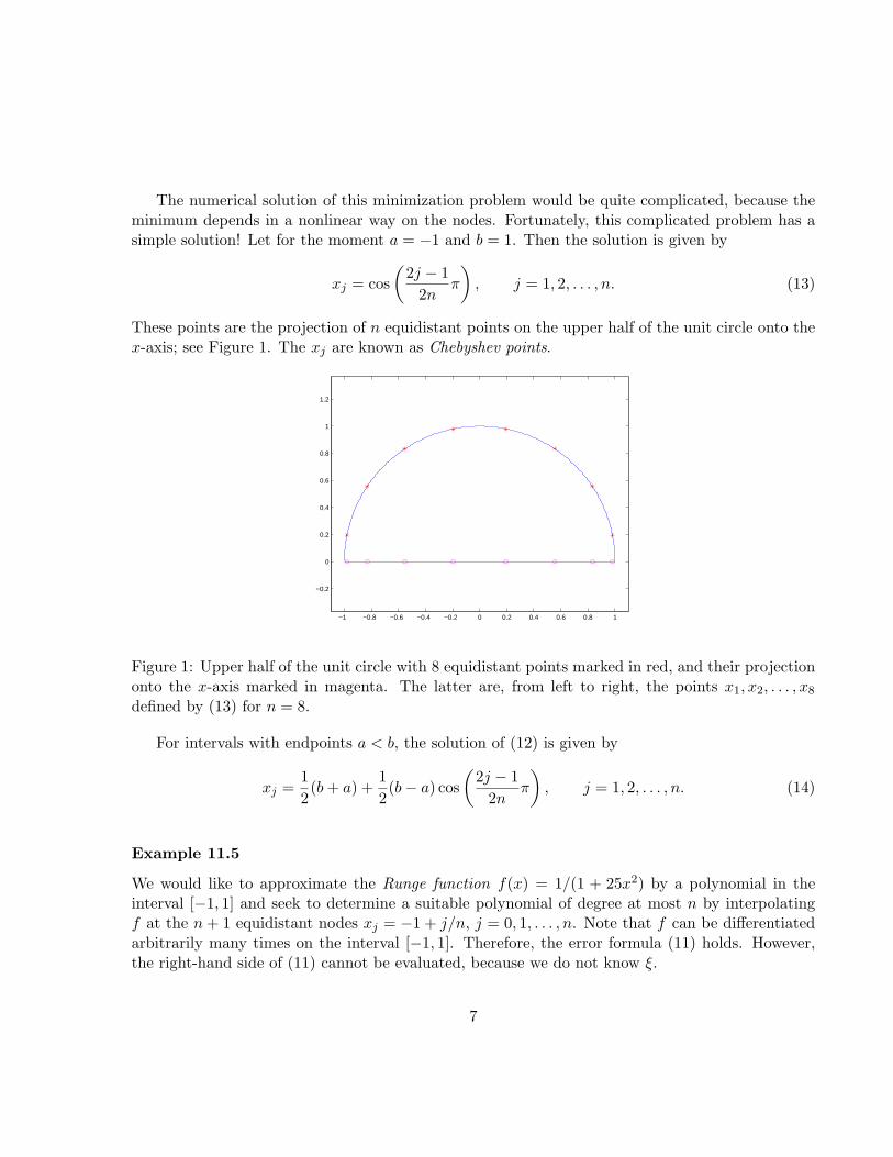
These points are the projection of n equidistant points on the upper half of the unit circle onto thex-axis; see Figure 1. The xj are known as Chebyshev points.

−1 −0.8 −0.6 −0.4 −0.2 0 0.2 0.4 0.6 0.8 1

−0.2

0

0.2

0.4

0.6

0.8

1

1.2

Figure 1: Upper half of the unit circle with 8 equidistant points marked in red, and their projectiononto the x-axis marked in magenta. The latter are, from left to right, the points x1, x2, . . . , x8

defined by (13) for n = 8.

For intervals with endpoints a < b, the solution of (12) is given by

xj =1

2(b + a) +

1

2(b − a) cos

(

2j − 1

2nπ

)

, j = 1, 2, . . . , n. (14)

Example 11.5

We would like to approximate the Runge function f(x) = 1/(1 + 25x2) by a polynomial in theinterval [−1, 1] and seek to determine a suitable polynomial of degree at most n by interpolatingf at the n + 1 equidistant nodes xj = −1 + j/n, j = 0, 1, . . . , n. Note that f can be differentiatedarbitrarily many times on the interval [−1, 1]. Therefore, the error formula (11) holds. However,the right-hand side of (11) cannot be evaluated, because we do not know ξ.

7

−1 −0.8 −0.6 −0.4 −0.2 0 0.2 0.4 0.6 0.8 1−0.2

0

0.2

0.4

0.6

0.8

1

1.2

−1 −0.8 −0.6 −0.4 −0.2 0 0.2 0.4 0.6 0.8 1−0.5

0

0.5

1

1.5

2

(a) (b)

−1 −0.8 −0.6 −0.4 −0.2 0 0.2 0.4 0.6 0.8 1−0.5

0

0.5

1

1.5

2

2.5

−1 −0.8 −0.6 −0.4 −0.2 0 0.2 0.4 0.6 0.8 1−60

−50

−40

−30

−20

−10

0

10

(c) (d)

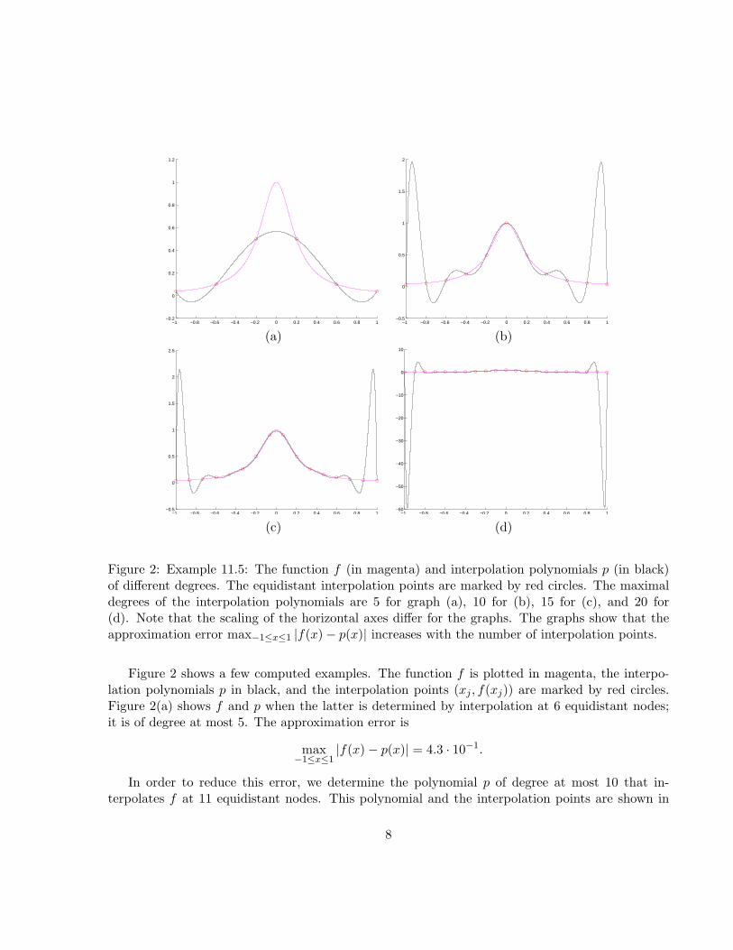
Figure 2: Example 11.5: The function f (in magenta) and interpolation polynomials p (in black)of different degrees. The equidistant interpolation points are marked by red circles. The maximaldegrees of the interpolation polynomials are 5 for graph (a), 10 for (b), 15 for (c), and 20 for(d). Note that the scaling of the horizontal axes differ for the graphs. The graphs show that theapproximation error max−1≤x≤1 |f(x) − p(x)| increases with the number of interpolation points.

Figure 2 shows a few computed examples. The function f is plotted in magenta, the interpo-lation polynomials p in black, and the interpolation points (xj , f(xj)) are marked by red circles.Figure 2(a) shows f and p when the latter is determined by interpolation at 6 equidistant nodes;it is of degree at most 5. The approximation error is

max−1≤x≤1

|f(x) − p(x)| = 4.3 · 10−1.

In order to reduce this error, we determine the polynomial p of degree at most 10 that in-terpolates f at 11 equidistant nodes. This polynomial and the interpolation points are shown in

8

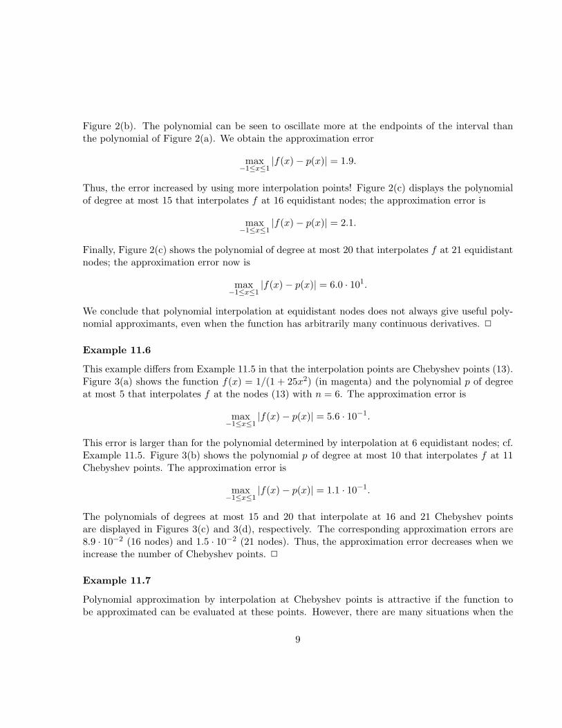
Figure 2(b). The polynomial can be seen to oscillate more at the endpoints of the interval thanthe polynomial of Figure 2(a). We obtain the approximation error

max−1≤x≤1

|f(x) − p(x)| = 1.9.

Thus, the error increased by using more interpolation points! Figure 2(c) displays the polynomialof degree at most 15 that interpolates f at 16 equidistant nodes; the approximation error is

max−1≤x≤1

|f(x) − p(x)| = 2.1.

Finally, Figure 2(c) shows the polynomial of degree at most 20 that interpolates f at 21 equidistantnodes; the approximation error now is

max−1≤x≤1

|f(x) − p(x)| = 6.0 · 101.

We conclude that polynomial interpolation at equidistant nodes does not always give useful poly-nomial approximants, even when the function has arbitrarily many continuous derivatives. 2

Example 11.6

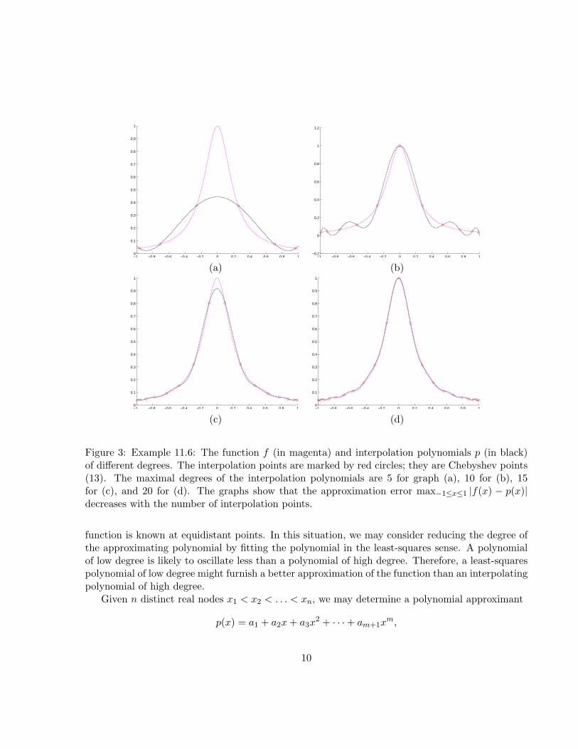
This example differs from Example 11.5 in that the interpolation points are Chebyshev points (13).Figure 3(a) shows the function f(x) = 1/(1 + 25x2) (in magenta) and the polynomial p of degreeat most 5 that interpolates f at the nodes (13) with n = 6. The approximation error is

max−1≤x≤1

|f(x) − p(x)| = 5.6 · 10−1.

This error is larger than for the polynomial determined by interpolation at 6 equidistant nodes; cf.Example 11.5. Figure 3(b) shows the polynomial p of degree at most 10 that interpolates f at 11Chebyshev points. The approximation error is

max−1≤x≤1

|f(x) − p(x)| = 1.1 · 10−1.

The polynomials of degrees at most 15 and 20 that interpolate at 16 and 21 Chebyshev pointsare displayed in Figures 3(c) and 3(d), respectively. The corresponding approximation errors are8.9 · 10−2 (16 nodes) and 1.5 · 10−2 (21 nodes). Thus, the approximation error decreases when weincrease the number of Chebyshev points. 2

Example 11.7

Polynomial approximation by interpolation at Chebyshev points is attractive if the function tobe approximated can be evaluated at these points. However, there are many situations when the

9

−1 −0.8 −0.6 −0.4 −0.2 0 0.2 0.4 0.6 0.8 10

0.1

0.2

0.3

0.4

0.5

0.6

0.7

0.8

0.9

1

−1 −0.8 −0.6 −0.4 −0.2 0 0.2 0.4 0.6 0.8 1−0.2

0

0.2

0.4

0.6

0.8

1

1.2

(a) (b)

−1 −0.8 −0.6 −0.4 −0.2 0 0.2 0.4 0.6 0.8 10

0.1

0.2

0.3

0.4

0.5

0.6

0.7

0.8

0.9

1

−1 −0.8 −0.6 −0.4 −0.2 0 0.2 0.4 0.6 0.8 10

0.1

0.2

0.3

0.4

0.5

0.6

0.7

0.8

0.9

1

(c) (d)

Figure 3: Example 11.6: The function f (in magenta) and interpolation polynomials p (in black)of different degrees. The interpolation points are marked by red circles; they are Chebyshev points(13). The maximal degrees of the interpolation polynomials are 5 for graph (a), 10 for (b), 15for (c), and 20 for (d). The graphs show that the approximation error max−1≤x≤1 |f(x) − p(x)|decreases with the number of interpolation points.

function is known at equidistant points. In this situation, we may consider reducing the degree ofthe approximating polynomial by fitting the polynomial in the least-squares sense. A polynomialof low degree is likely to oscillate less than a polynomial of high degree. Therefore, a least-squarespolynomial of low degree might furnish a better approximation of the function than an interpolatingpolynomial of high degree.

Given n distinct real nodes x1 < x2 < . . . < xn, we may determine a polynomial approximant

p(x) = a1 + a2x + a3x2 + · · · + am+1x

m,

10

−1 −0.8 −0.6 −0.4 −0.2 0 0.2 0.4 0.6 0.8 1−0.2

0

0.2

0.4

0.6

0.8

1

1.2

−1 −0.8 −0.6 −0.4 −0.2 0 0.2 0.4 0.6 0.8 10

0.1

0.2

0.3

0.4

0.5

0.6

0.7

0.8

0.9

1

(a) (b)

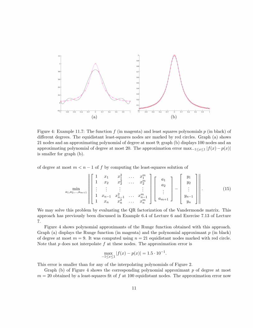
Figure 4: Example 11.7: The function f (in magenta) and least squares polynomials p (in black) ofdifferent degrees. The equidistant least-squares nodes are marked by red circles. Graph (a) shows21 nodes and an approximating polynomial of degree at most 9; graph (b) displays 100 nodes and anapproximating polynomial of degree at most 20. The approximation error max−1≤x≤1 |f(x)− p(x)|is smaller for graph (b).

of degree at most m < n − 1 of f by computing the least-squares solution of

mina1,a2,...,am+1

∥

∥

∥

∥

∥

∥

∥

∥

∥

∥

∥

1 x1 x21 . . . xm

1

1 x2 x22 . . . xm

2...

......

...1 xn−1 x2

n−1 . . . xmn−1

1 xn x2n . . . xm

n

a1

a2...

am+1

−

y1

y2...

yn−1

yn

∥

∥

∥

∥

∥

∥

∥

∥

∥

∥

∥

. (15)

We may solve this problem by evaluating the QR factorization of the Vandermonde matrix. Thisapproach has previously been discussed in Example 6.4 of Lecture 6 and Exercise 7.13 of Lecture7.

Figure 4 shows polynomial approximants of the Runge function obtained with this approach.Graph (a) displays the Runge function (in magenta) and the polynomial approximant p (in black)of degree at most m = 9. It was computed using n = 21 equidistant nodes marked with red circle.Note that p does not interpolate f at these nodes. The approximation error is

max−1≤x≤1

|f(x) − p(x)| = 1.5 · 10−1.

This error is smaller than for any of the interpolating polynomials of Figure 2.Graph (b) of Figure 4 shows the corresponding polynomial approximant p of degree at most

m = 20 obtained by a least-squares fit of f at 100 equidistant nodes. The approximation error now

11

is somewhat smaller:max

−1≤x≤1|f(x) − p(x)| = 1.4 · 10−1.

One can show that if the degree m of the least-squares polynomial p is chosen about 2√

n,where n is the number of equidistant nodes, then the approximation error converges to zero as nis increased. However, as this example illustrates, the rate of convergence is not very fast. 2

Despite the difficulties to determine an accurate polynomial approximant of the Runge functionon [−1, 1] by interpolation at equidistant nodes, for some functions, including ex, sin(x), and cos(x),the interpolation polynomials converge to the function on [−1, 1] for all distributions of distinctinterpolation points on the interval [−1, 1] as the number of points is increased. For definiteness,consider f(x) = ex and let x1 < x2 < . . . < xn be arbitrary distinct points in [−1, 1]. We obtainfrom (11) that

max−1≤x≤1

|f(x) − p(x)| = max−1≤x≤1

|n

∏

j=1

(x − xj)||f (n)(ξ)|

n!

≤ max−1≤x≤1

n∏

j=1

|x − xj | max−1≤x≤1

|f (n)(ξ)|n!

. (16)

Since x, xj ∈ [−1, 1], we have |x − xj | ≤ 2. Therefore,

max−1≤x≤1

n∏

j=1

|x − xj | ≤ 2n.

Moreover, f (n)(ξ) = eξ with −1 ≤ ξ ≤ 1. Therefore, |f (n)(ξ)| ≤ e. Substituting these bounds into(16) shows that

max−1≤x≤1

|f(x) − p(x)| = max−1≤x≤1

|n

∏

j=1

(x − xj)||f (n)(ξ)|

n!≤ e

2n

n!.

The right-hand side converges to zero as n increases, because n! grows much faster with n than 2n.This shows that we can determine an arbitrarily accurate polynomial approximation of ex on theinterval [−1, 1] by polynomial interpolation at arbitrary distinct nodes in the interval.

The fact that we obtain convergence for arbitrary distinct interpolation points, does not implythat all distributions of interpolation points the same approximation error. This will be exploredfurther in Exercise 11.9.

The presence of a high-order derivative in the error-formula (11) indicates that interpolationpolynomials are likely to give small approximation errors when the function has many continuousderivatives that are not very large in magnitude. Conversely, equation (11) suggests that interpo-lating a function with few or no continuous derivatives in [a, b] by a polynomial of small to moderate

12

degree might not yield an accurate approximation of f(x) on [a, b]. This, indeed, often is the case.We therefore in the next section discuss an extension of polynomial interpolation which typicallygives more accurate approximations than standard polynomial interpolation when the function tobe approximated is not smooth.

Exercise 11.1

Solve the interpolation problem of Example 11.1. 2

Exercise 11.2

Write a MATLAB/Octave function for evaluating the polynomial in nested form (4). The inputare the coefficients aj and x; the output is the value p(x). 2

Exercise 11.3

Let Vn be an n×n Vandermonde matrix determined by n equidistant nodes in the interval [−1, 1].How quickly does the condition number of Vn grow with n? Linearly, quadratically, cubically,. . ., exponentially? Use the MATLAB/Octave functions vander and cond. Determine the growthexperimentally. Describe how you designed the experiments. Show your MATLAB/Octave codesand relevant input and output. 2

Exercise 11.4

Show that the Lagrange polynomials (5) satisfy

n∑

j=1

ℓj(x) = 1

for all x. Hint: Which function does the sum interpolate? Use the unicity of the interpolationpolynomial. 2

Exercise 11.5

Write a MATLAB/Octave function for computing the weights of the barycentric representation(10) of the interpolation polynomial, using the definition (8). The code should avoid overflow andunderflow. 2

Exercise 11.6

Given the weights (8), write a MATLAB/Octave function for evaluating the polynomial (10) at apoint x. 2

13

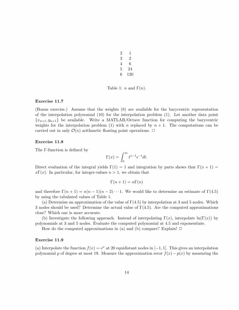
2 13 24 65 246 120

Table 1: n and Γ(n).

Exercise 11.7

(Bonus exercise.) Assume that the weights (8) are available for the barycentric representationof the interpolation polynomial (10) for the interpolation problem (1). Let another data point{xn+1, yn+1} be available. Write a MATLAB/Octave function for computing the barycentricweights for the interpolation problem (1) with n replaced by n + 1. The computations can becarried out in only O(n) arithmetic floating point operations. 2

Exercise 11.8

The Γ-function is defined by

Γ(x) =

∫ ∞

0tx−1e−tdt.

Direct evaluation of the integral yields Γ(1) = 1 and integration by parts shows that Γ(x + 1) =xΓ(x). In particular, for integer-values n > 1, we obtain that

Γ(n + 1) = nΓ(n)

and therefore Γ(n + 1) = n(n − 1)(n − 2) · · · 1. We would like to determine an estimate of Γ(4.5)by using the tabulated values of Table 1.

(a) Determine an approximation of the value of Γ(4.5) by interpolation at 3 and 5 nodes. Which3 nodes should be used? Determine the actual value of Γ(4.5). Are the computed approximationsclose? Which one is more accurate.

(b) Investigate the following approach. Instead of interpolating Γ(x), interpolate ln(Γ(x)) bypolynomials at 3 and 5 nodes. Evaluate the computed polynomial at 4.5 and exponentiate.

How do the computed approximations in (a) and (b) compare? Explain! 2

Exercise 11.9

(a) Interpolate the function f(x) = ex at 20 equidistant nodes in [−1, 1]. This gives an interpolationpolynomial p of degree at most 19. Measure the approximation error f(x)− p(x) by measuring the

14

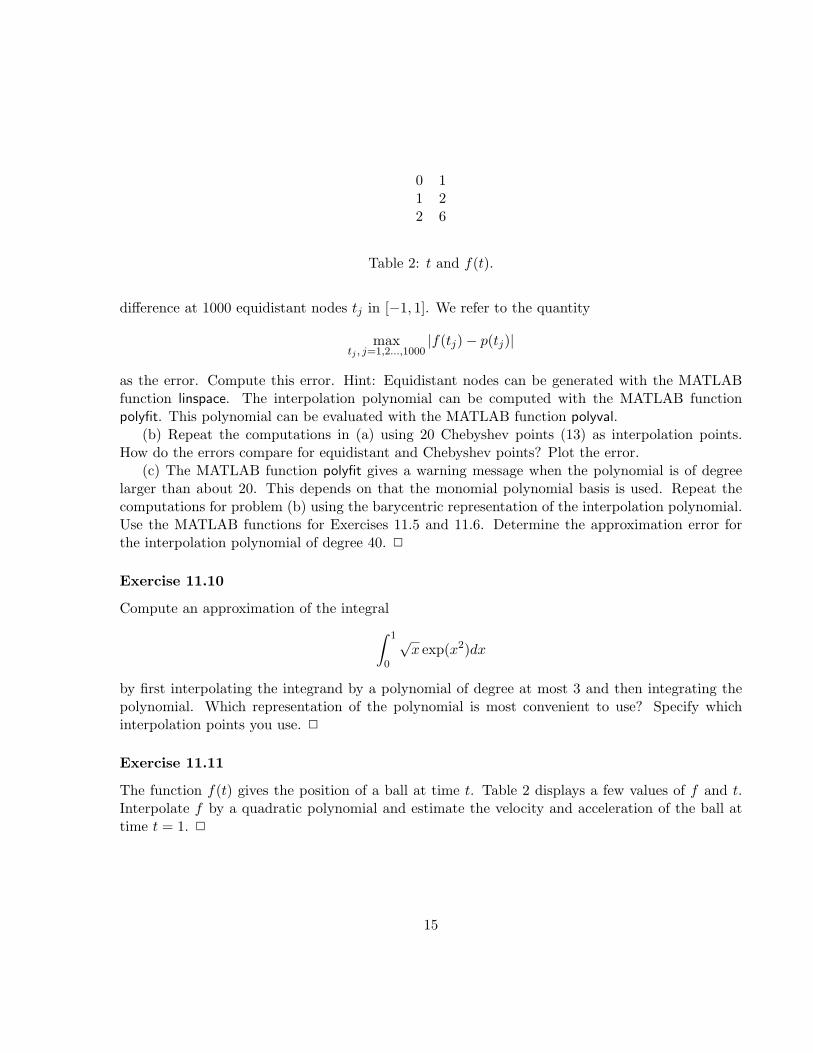
0 11 22 6

Table 2: t and f(t).

difference at 1000 equidistant nodes tj in [−1, 1]. We refer to the quantity

maxtj , j=1,2...,1000

|f(tj) − p(tj)|

as the error. Compute this error. Hint: Equidistant nodes can be generated with the MATLABfunction linspace. The interpolation polynomial can be computed with the MATLAB functionpolyfit. This polynomial can be evaluated with the MATLAB function polyval.

(b) Repeat the computations in (a) using 20 Chebyshev points (13) as interpolation points.How do the errors compare for equidistant and Chebyshev points? Plot the error.

(c) The MATLAB function polyfit gives a warning message when the polynomial is of degreelarger than about 20. This depends on that the monomial polynomial basis is used. Repeat thecomputations for problem (b) using the barycentric representation of the interpolation polynomial.Use the MATLAB functions for Exercises 11.5 and 11.6. Determine the approximation error forthe interpolation polynomial of degree 40. 2

Exercise 11.10

Compute an approximation of the integral

∫ 1

0

√x exp(x2)dx

by first interpolating the integrand by a polynomial of degree at most 3 and then integrating thepolynomial. Which representation of the polynomial is most convenient to use? Specify whichinterpolation points you use. 2

Exercise 11.11

The function f(t) gives the position of a ball at time t. Table 2 displays a few values of f and t.Interpolate f by a quadratic polynomial and estimate the velocity and acceleration of the ball attime t = 1. 2

15

11.3 Interpolation by piecewise polynomials

In the above section, we sought to determine one polynomial that approximates a function on aspecified interval. This works well if either one of the following conditions hold:

• The polynomial required to achieve desired accuracy is of fairly low degree.

• The function has several continuous derivatives and interpolation can be carried out at theChebyshev points (13) or (14).

A quite natural and different approach to approximate a function on an interval is to first splitthe interval into subintervals and then approximate the function by a polynomial of fairly lowdegree on each subinterval. The present section discusses this approach.

Example 11.8

We would like to approximate a function on the interval [−1, 1]. Let the function values yj = f(xj)be available, where x1 = −1, x2 = 0, x3 = 1, and y1 = y3 = 0, y2 = 1. It is easy to approximatef(x) by a linear function on each subinterval [x1, x2] and [x2, x3]. We obtain, using the Lagrangeform (7),

p(x) = y1x − x2

x1 − x2+ y2

x − x1

x2 − x1= x + 1, −1 ≤ x ≤ 0,

p(x) = y2x − x3

x2 − x3+ y3

x − x2

x3 − x2= 1 − x, 0 ≤ x ≤ 1.

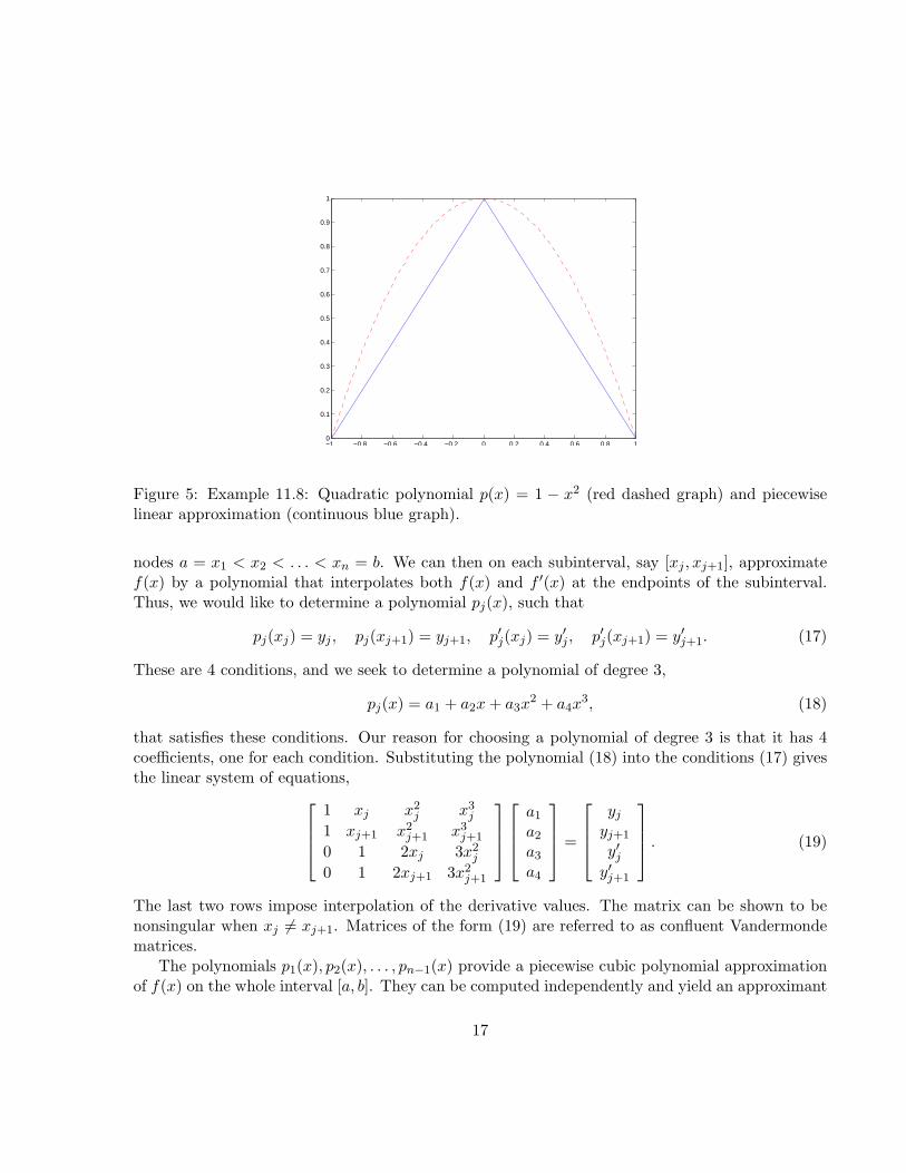
The MATLAB command plot([-1,0,1],[0,1,0]) gives the continuous graph of Figure 5. This is apiecewise linear approximation of the unknown function f(x). If f(x) indeed is a piecewise linearfunction with a kink at x = 0, then the computed approximation is appropriate, On the otherhand, if f(x) displays the trajectory of a baseball, then the smoother function p(x) = 1−x2, whichis depicted by the dashed curve, may be a more suitable approximation of f(x), since baseballtrajectories do not exhibit kinks - even if some players occasionally may wish they do.

Piecewise linear functions give better approximations of a smooth function if more interpolationpoints {xj , yj} are used. We can increase the accuracy of the piecewise linear approximant byreducing the lengths of the subintervals and thereby increasing the number of subintervals.

We conclude that piecewise linear approximations of functions are easy to compute. However,piecewise linear approximants display kinks. Therefore, many subintervals may be required todetermine a piecewise linear approximant of high accuracy. 2

There are several ways to modify piecewise linear functions to give them a more pleasing look.Here we will discuss how to use derivative information to obtain smoother approximants. A differentapproach, which uses Bezier curves, is described in Lecture 12.

We consider the task of approximating a function on the interval [a, b] and first assume that notonly the function values yj = f(xj), but also the derivative values y′j = f ′(xj), are available at the

16

−1 −0.8 −0.6 −0.4 −0.2 0 0.2 0.4 0.6 0.8 10

0.1

0.2

0.3

0.4

0.5

0.6

0.7

0.8

0.9

1

Figure 5: Example 11.8: Quadratic polynomial p(x) = 1 − x2 (red dashed graph) and piecewiselinear approximation (continuous blue graph).

nodes a = x1 < x2 < . . . < xn = b. We can then on each subinterval, say [xj , xj+1], approximatef(x) by a polynomial that interpolates both f(x) and f ′(x) at the endpoints of the subinterval.Thus, we would like to determine a polynomial pj(x), such that

pj(xj) = yj , pj(xj+1) = yj+1, p′j(xj) = y′j , p′j(xj+1) = y′j+1. (17)

These are 4 conditions, and we seek to determine a polynomial of degree 3,

pj(x) = a1 + a2x + a3x2 + a4x

3, (18)

that satisfies these conditions. Our reason for choosing a polynomial of degree 3 is that it has 4coefficients, one for each condition. Substituting the polynomial (18) into the conditions (17) givesthe linear system of equations,

1 xj x2j x3

j

1 xj+1 x2j+1 x3

j+1

0 1 2xj 3x2j

0 1 2xj+1 3x2j+1

a1

a2

a3

a4

=

yj

yj+1

y′jy′j+1

. (19)

The last two rows impose interpolation of the derivative values. The matrix can be shown to benonsingular when xj 6= xj+1. Matrices of the form (19) are referred to as confluent Vandermondematrices.

The polynomials p1(x), p2(x), . . . , pn−1(x) provide a piecewise cubic polynomial approximationof f(x) on the whole interval [a, b]. They can be computed independently and yield an approximant

17

that is continuous and has a continuous derivative on [a, b]. The latter can be established asas follows: The polynomial pj is defined and differentiable on the subinterval [xj , xj+1] for j =1, 2, . . . , n−1. What remains to be shown is that our approximant is continuous and has a continuousderivative at the interpolation points. This follows from the interpolation conditions (17). We have

limxրxj+1

pj(x) = pj(xj+1) = yj+1, limxցxj+1

pj+1(x) = pj+1(xj+1) = yj+1

andlim

xրxj+1

p′j(x) = p′j(xj+1) = y′j+1, limxցxj+1

p′j+1(x) = p′j+1(xj+1) = y′j+1.

The existence of the limits follows from the continuity of each polynomial and its derivative on thesubinterval where it is defined. Thus,

pj(xj+1) = pj+1(xj+1), p′j(xj+1) = p′j+1(xj+1).

This shows the continuity of our piecewise cubic polynomial approximant and its derivative at xj+1.The use of piecewise cubic polynomials as described gives attractive approximations. However,

the approach discussed requires that derivative information be available. When no derivative infor-mation is explicitly known, modifications of the scheme outlined can be used. A simple modificationis to use estimates the derivative-values of the function f(x) at the nodes; see Exercise 11.13.

A popular approach to determine a smooth piecewise polynomial approximant is to use splines.Again consider the problems of approximation a function f on the interval [a, b] and assume thatfunction values yj = f(xj) are known at the nodes a = x1 < x2 < . . . < xn−1 < xn = b, but thatno derivative information is available. We then impose the conditions p1(x1) = y1 and

pj(xj) = yj , pj(xj+1) = yj+1, p′j(xj) = p′j−1(xj), p′′j (xj) = p′′j−1(xj),

for j = 2, 3, . . . , n−1. Thus, at the subinterval boundaries at x2, x3, . . . , xn−1, we require the piece-wise cubic polynomial to have continuous first and second derivatives. However, these derivativesare not required to take on prescribed values. This kind of piecewise cubic polynomials are knownas (cubic) splines. They are popular design tools in industry. Their determination requires the so-lution of a linear system of equations, which is somewhat complicated to derive. We will thereforeomit its derivation. Extra conditions at the endpoints a and b have to be imposed in order to makethe resulting linear system of equations uniquely solvable. For instance, we may require that thesecond derivative of the spline vanishes at a and b. These are referred to as “natural” boundaryconditions. Alternatively, if the derivative of the function to be approximated is known at a andb, then we may require that the derivative of the spline takes on these values. If the function f isperiodic with period b − a, then it can be attractive to require the first and second derivative alsobe periodic.

18

Exercise 11.12

Consider the function in Example 11.8. Assume that we also know the derivative values y′1 = 2,y′2 = 0, and y′3 = −2. Determine a piecewise polynomial approximation on [−1, 1] by using theinterpolation conditions (17). Plot the resulting function. 2

Exercise 11.13

Assume the derivative values in the above exercise are not available. How can one determineestimates of these values? Use these estimates in the interpolation conditions (17) and compute apiecewise cubic approximation. How does it compare with the one from Exercise 11.12 and withthe piecewise linear approximation of Example 11.8. Plot the computed approximant. 2

Exercise 11.14

Compute a spline approximant of the function of Example 11.8, e.g., by using the function splinein MATLAB or Octave. Plot the computed spline. 2

Exercise 11.15

Compute a spline approximant of the function of Example 11.5 using 20 equidistant nodes e.g.,by using the function spline in MATLAB or Octave. Plot the computed spline. Compute theapproximation error similarly as in Example 11.5. 2

19