polynomial filtering: to any degree on irregularly sampled data

Pieter V. Reyneke, Norman Morrison, Derrick G. Kourie, Corné de Ridder

Polynomial Filtering: To any degree on irregularly sampled data

DOIUDKIFAC

10.7305/automatika.53-4.248621.372.852.1:519.2/.6;621.396.969.35.8.3; 1.1 Original scientific paper

Conventionally, polynomial filters are derived for evenly spaced points. Here, a derivation of polynomial filtersfor irregularly spaced points is provided and illustrated by example. The filter weights and variance reductionfactors (VRFs) for both expanding memory polynomial (EMP) and fading-memory polynomial (FMP) filters areprogrammatically derived so that the expansion up to any degree can be generated. (Matlab was used for doingthe symbolic weight derivations utilizing Symbolic Toolbox functions.) Order-switching and length-adaption arebriefly considered. Outlier rejection and Cramer-Rao Lower Bound consistency are touched upon. In terms ofperformance, the VRF and its decay for the EMP filter is derived as a function of length (n) and the switch-overpoint is calculated where the VRFs of the EMP and FMP filters are equal. Empirical results verifying the derivationand implementation are reported.

Key words: Radar tracking filters, Polynomial approximation, Smoothing, State estimation, Satellite tracking,Discrete time filters, Laguerre processes, Legendre processes, Polynomial approximation, Smooth-ing methods, Interpolation, Extrapolation

Polinomno filtriranje: postizanje bilo kojeg stupnja na nepravilno uzorkovanim podacima. Polinomni filtriuobicajeno se rade za ravnomjerno rasporedene tocke u prostoru. U ovom radu dana je derivacija polinomnih filtaraza neravnomjerno rasporedene tocke. Težinske vrijednosti filtra i faktori smanjenja varijance (VRF-ovi) za polinomproširene memorije (EMP) i polinom oslabljenje memorije (FMP) su programski podržani tako da se može napravitiekspanzija do bilo kojeg stupnja. Kratko su razmotreni i promjena poretka i adaptacija dužine filtra. Dotaknute sui metode odbijanja jako raspršenih rezultata i Cramer-Raove konzistencije donje granice. VRF i njegovo opadanjeza EMP filtar izvedeno je kao funkcija duljine (n) i izracunata je tocka prijelaza gdje su VRF-ovi od EMP i FMPfiltara jednaki. Predoceni su empirijski rezultati koji verificiraju izvod i implementaciju.

Kljucne rijeci: filtri za pracenje radara, polinomna aproksimacija, izgladivanje, procjena stanja, pracenje satelita,diskretni vremenski filtri, Laguerreovi procesi, Legendreovi procesi, aproksimacija polinomom,metode izgladivanja, interpolacija, ekstrapolacija

1 INTRODUCTION

The 1-step predictor and current-estimate filters intro-duced by Morrison in [1] and [2] both recursively calculatea least squares approximation of a process model, in ef-fect determining the state of a polynomial curve fitted overnoisy input observations. The origin of the fitted curve ison the last added observation’s timestamp.

The expanding memory polynomial filter (EMP) ad-heres to the Cramér-Rao lower bound (CRLB1) on vari-ance, thus it is CRLB consistent [2]. However, the fadingmemory polynomial filter (FMP) is not CRLB consistent.

1The Cramér-Rao lower bound is a limit to the variance that can beattained by a linear unbiased estimator of a parameter of a distribution.See [3], [4] for fundamentals, [5] for a well-explained application and [1]for the proof of CRLB consistency, specifically for polynomial filters.

In the present context, recursive refers to adding oneobservation at a time. To date these filters have been sub-ject to the constraint that observations have to be evenlyspaced. However, in natural environments, measurementscannot always be assigned to an integer type time batchwithout losing accuracy. Reasons therefore are threefold:

• Floating point time values more accurately positionupdates in time, leading to less ambiguity caused bynatural variations (related to, for example, tempera-ture, target clutter, occlusions, etc.).

• Detector or algorithm design may result in non-deterministic jumps in the update intervals, or inuneven even/odd time-interval symmetry. Exampleswhere variable update intervals can be expected in-clude: nodding algorithms, zig-zag sweep detectors,linear sensor integration and asynchronous mode

Online ISSN 1848-3380, Print ISSN 0005-1144ATKAFF 53(4), 382–397(2012)

382 AUTOMATIKA 53(2012) 4, 382–397

Polynomial Filtering P. V. Reyneke, N. Morrison, D. G. Kourie, C. de Ridder

changing.

For the above mentioned reasons this research proposesa variable-step extension to the polynomial filters derivedin [1] and [2], refining the proposed filters in [6].

The biggest advantage of recursive EMP and FMP fil-ters, other than being extremely fast, is that their use ofdiscrete orthogonal basis functions eliminates the need formatrix inversions in the auto-regression (AR) process.

We prefer to distinguish between orthogonal and or-thonormal function sets, although orthogonal is the termgenerally attributed to a function set being both orthog-onal and normalised. This opinion is becoming generallyacceptable and is reflected by Chihara in [7].

NOMENCLATURE

In what follows, the following notation is used:

• t represents time in seconds;• τ represents the constant expected update period (or

system batch time) in seconds;• δ represents delta-time in seconds;• η (a real value) represents time in τ ’s;• ζ (a real value) represents delta-time in τ ’s;• Z the state on the last timestamp, the coefficients of a

polynomial function; and• Z∗ the estimated state at a time other than the last

timestamp.

Additionally, the term order is used to refer to a non-negative integer value attributed to a fit, a differential equa-tion, a process model or a filter model; and the term degreeis used to refer to a value attributed to a polynomial.

The remainder of this article is laid out as follows. Sec-tion 2 points to application areas for the proposed filteringtechnique. As background Section 3 provides a solutionto the classical linear tracking differential equation and inSection 4 a motivation for a change in the state transitionmatrix is presented. An overview of the solutions for twodiscrete orthonormal (DON) polynomial function sets isgiven in Sections 5.1 and 5.2 respectively. Furthermore it isshown in Section 5.3 that matrix-inversion can be avoided.Section 5 provides the underpinnings of Section 6. An ex-planation of the extension of the current-estimate filter toa variable-step polynomial filter is given in Section 6.1.Thereafter recursive weight updates for the EMP and FMPfilters are symbolically derived from the DON polyno-mials. Section 7 provides methods of auto-initialisation,combining, length-adaption and order switching for poly-nomial filters. Section 8 reports on results obtained fromtrial runs on simulated polynomial data thereby verifyingthe prediction capability of a variable-step implementation.

The smoothing results on noisy, irregular, real data can befound in 8.2. Results obtained during missile testing areprovided in 8.3. The article is concluded in Section 9.

To enhance the flow of the article, all relevant Matlabcode has been included in APPENDIX A. The reader isreferred to the code where applicable.

2 APPLICATION AREAS

Apart from the application areas dealing with irregu-larly updating sensors mentioned in Section 1, two othertypes of application areas can be distinguished: firstly, ar-eas where polynomial filtering to a higher degree may berequired; and secondly, areas where extremely fast execu-tion speed are required.

Polynomial fit application areas where PFs to a higherdegree were successfully demonstrated include:

(a.) Plant Control: when measurement noise in plant mon-itoring systems is low enough, higher degree fittingand predicting becomes feasible. New dynamic be-havior can be observed in this manner.

(b.) In inertial kinematics, position derivatives are alreadydefined up to the sixth order, as follows: velocity (1st),acceleration (2nd), jerk (3rd), snap (4th), crackle (5th)and pop (6th), terminology proposed by Gibbs andGragert in 1996 [8]. These may require estimation andplotting in the near future.

(c.) In structural dynamics, e.g. earth quake modeling,higher degree fits may increase measurement andmodeling accuracy.

(d.) Finally, in tracking, if higher degrees are observablein the underlying truth of a tracking scenario then, de-pending on system noise levels, one can consider in-creasing the memory timespan and doing a higher de-gree fit than four. This is especially true in 2D imagingsystems where very high dynamic behavior is observ-able in the end game of such target intercept systems.Furthermore in 3D systems higher degree estimationenables the tracking of sinusoidal functions and hencecircular manoeuvres more accurately.

Note that one should be careful not to use a higher de-gree filter than the natural degree present in the underly-ing truth of the controlled system, or points to be approxi-mated.

The proposed variable-step filters have been applied intwo areas where extremely fast execution speeds are re-quired:

AUTOMATIKA 53(2012) 4, 382–397 383


(a.) Image integration: An array of more than 10 000 poly-nomial filters was recently used to integrate and aver-age an imaging sensor with a longish history length of200 frames. Subtracting the averaged image from thecurrent led to improved Signal-to-Noise ratio and sup-pressed unwanted artifacts. The successfully demon-strated filter array may be implemented in VHDL tolessen processing load maintaining the required real-time processing requirement.

(b.) Constant false-alarm rate (CFAR) mean estimatorfilters for LADAR ranging and range-gate applica-tions require fast robust pulse detection for time-of-flight measurement and pulse repetition interval (PRI)tracking. Signals are commonly sampled at above 2Gsamples/s. The CFAR commonly thresholds any de-viation of more than 3σ from a mean. PFs can be usedas a good mean-estimator for the segmenting, detec-tion and tracking of wanted pulses.

3 MODELING A CLASSICAL DIFFERENTIALEQUATION

To explain polynomial filters, consider modeling theclassical 2nd-order linear differential equation (DE), whereit is assumed that the 3rd derivative is 0.

r =dr

dtr =

dr

dt

...r =

dr

dt= 0 (1)

If r is defined as r = [r1, r2, r3]T = [r, r, r]T , the DEbecomes:

r1 = r2 r2 = r3 r3 = 0 (2)

This may be written in matrix form as follows:

r = Ar (3)

where:

A =

[0 1 00 0 10 0 0

](4)

Note that r = Z, which is the nth order state vector.

Ψ(t) = eAt is a solution for the linear DE system inEquation 3. The system has infinitely many solutions de-pending on the initial conditions. Note that Ψ(δ) can beused as a state transition matrix (STM). An STM is used toshift the validity instant of a DE system’s state vector fromtime t by an amount δ, a real number, to time t + δ via asimple matrix multiplication (Equation 6).

Thus prediction can be done without recalculating thestate (Z). By using the STM one can shift the state alongtime as follows: Z∗(t+ δ) = Ψ(δ)Z(t). Note, the asteriskindicates that the newly calculated state is an estimate at

t + δ. The asterisk is omitted at t since t is where the lastfit was calculated.

One can either choose the Padé expanded STM, Ψ(δ),or the commonly used STM for polynomial filteringΦ(δ), [1, 6]. We prefer using the Padé expanded STM forthe derivation. (See Section 4.)

The linear DE in Equation 3 has the following discretesolution [9] :

z(t+ δ) = Ψ(δ)z(t) (5)

The state transition matrix Ψ(δ)2, for the 2nd-order DE inEquation 3, is:

Ψ(δ) =

1 δ δ2

2!0 1 δ0 0 1

(6)

and as will be seen, Equation 37, written out for the 2nd

order variable-step filter update, renders:

z2t = z∗2 t,t−δ + 2!Γ2en

z1t = z∗1 t,t−δ + Γ1en

z0t = z∗0 t,t−δ + Γ0en

where the Γ’s for the 2nd-degree for EMP and FMP foruse with the Ψ are simply (see Sections 6.4 and 6.6):

Γ2(n) = (2!)30

(n+3)(3)Γ2(θ) = 2!(1−θ)3

2

Γ1(n) = 18(2n+1)

(n+3)(3)Γ1(θ) = 3

2(1− θ)2(1 + θ)

Γ0(n) = 3(3n2+3n+2)

(n+3)(3)Γ0(θ) = 1− θ3

Note that the EMP filter is self-initializing and can beswitched with no degrading effects to the FMP filter atthe instant when their variance reduction factors (VRF) areequal. (See Section 7.2.) Because of its fading memory, theFMP filter effectively possesses a fixed memory3, and so ithas the advantage of being able to follow sinusoids. It cantherefore be used to approximate circular trends as well.

4 THE TWO STATE TRANSITION MATRICESFROM WHICH TO CHOOSE

An STM is used to shift a DE system’s state vector fromtime t by an amount δ, a real number, to time t + δ via asimple multiplication. This is done without recalculatingthe state (Z). Thus, using the STM one can shift the state

2The original expanding memory polynomial (EMP) and fading mem-ory polynomial (FMP) filters as derived in Chapters 9 and 13 of [2], canbe adapted to utilise the STM in Equation 7. ΓΨ can be written in termsof Γ(=ΓΦ) as follows ΓΨ(j, i) = ΓΦ(j, i) × (i− j)!, see [6].

3The history in the FMP filter’s case is discounted by the ratio θ perupdate or over time. For example the value 0.91, if done per update, repre-sents an approximate memory length of around 30 samples. The formulaN = 2/(1− θ) may be used to calculate an approximate effective mem-ory length for the FMP filter for 0th order, see Section 7.2 for higherorders.

384 AUTOMATIKA 53(2012) 4, 382–397


as follows: Z∗(t+ δ) = Ψ(δ)Z(t). Note, the asterisk indi-cates that the newly calculated state is an estimate at t+ δ.The asterisk is omitted at t since t is where the last fit wascalculated.

As the STM of the polynomial one can either choose thePadé expanded STM, Ψ(δ), or the commonly used STMfor polynomial filtering Φ(δ). (See [1].) Both can be useddirectly for prediction of states at any time, with or withoutdenormalisation. For example in our case, as will be seen,Zn∗ could be predicted from Zη−ζ directly before updat-

ing the state, where η = tτ with τ a real positive number,

and ζ = δτ .

Note that [9] compares many algorithms for computingthe matrix exponential. (See the expm function in [10].)

The Padé expanded STM is:

[Ψ(δ)]i,j =δj−i

(j − i)!{∀ i, j| 0 ≤ i ≤ j ≤ m}

0 elsewhere(7)

where m = order + 1 is the dimension of the squarematrix Ψ.

This transition matrix (exactly the same as the one well-known from least squares), can be written out as follows:

Ψ(δ) =

1 δ δ2

2!· · · δm−1

(m−1)!δm

m!

0 1 δ · · · δm−2

(m−2)!δm−1

(m−1)!

0 0 1 · · · δm−3

(m−3)!δm−2

(m−2)!

......

.... . .

......

0 0 0 · · · 1 δ0 0 0 · · · 0 1

(8)

The commonly used STM for polynomial filtering, definedin [1], is represented as follows:

Φi,j(δ) =

(j

i

)δ(j−i)

{∀ i, j| 0 ≤ i ≤ j ≤ m}

0 elsewhere(9)

=j!

(j − i)!i!δ(j−i) (10)

where m = order + 1 is the dimension of the squarematrix Φ.

This original transition matrix, in Equation 10, can bewritten out as follows:

Φ(δ) =

1 δ δ2 · · · m−1!(m−2)!1!

δm−2 m!(m−1)!1!

δm−1

0 1 δ · · · m−1!(m−3)!2!

δm−3 m!(m−2)!2!

δm−2

0 0 1 · · · m−1!(m−4)!3!

δm−4 m!(m−3)!3!

δm−3

......

.... . .

......

0 0 0 · · · 1 δ0 0 0 · · · 0 1

(11)

The following discrete system results from the commonlyused STM:

r(t+ δ) = Φ(δ))r(t) or in normalized form (12)r(t+ δ) = DΦ(τ)Φ(ζ)r(η) (13)

where DΦ(τ) = diag([

1 1!τ . . . m!

τm

]) is the di-

agonal denormalisation matrix for Φ, described in [1] andthis matrix is slightly different from the DΨ(τ) denormal-isation in Section 6.1, Equation 33.

We prefer to utilize and extend the first STM option,presented in Equation 7 and written out in Equation 8,because Ψ(δ) can easily be differentiated by simply usingonly one less row and column of Ψ(δ), e.g. in Matlab:z_dot = Psi(1:N-1,1) * z'(2:N);. The sameholds for higher order derivatives. This characteristic isalso applicable to the multi-dimensional case.

Altering the original EMP and FMP to use with Ψ:The original EMP and FMP filters as derived in Chap-

ters 9 and 13 of [2], can be adapted to utilise the STM inEquation 7.

ΓΨ, the weight for updating the Ψ STM based filter, isdefined in terms of Γ(= ΓΦ), the weight for updating theoriginal Φ STM based filter, for the ith-degree polynomialset for both the EMP and FMP filters, as follows:

ΓΨ(j, i) = ΓΦ(j, i)× (i− j)!

where j ∈ [0, i].As an example, the change for the 4th degree ΓΨ is:

ΓΨ(4, 4) = αΨ = α× 0!

ΓΨ(3, 4) = βΨ = β × 1!

ΓΨ(2, 4) = γΨ = γ × 2!

ΓΨ(1, 4) = δΨ = δ × 3!

ΓΨ(0, 4) = εΨ = ε× 4!

(See Sections 3, 6.4 and 6.6)Furthermore, denormalisation of obtained normalised

(i.e. τ 6= 1) state-vectors is done by either pre-multiplyingthe state, by DΦ(τ) for Φ (see Equation 13); or by DΨ(τ)if using the Ψ STM choice (see Equation 36). See Section 6for a description.

5 TWO DISCRETE ORTHONORMAL (DON)POLYNOMIAL SETS

Discrete orthogonal polynomials are encountered in dis-crete probability theory. The weights of the Chebyshev,Krawtchouk, and Charlier polynomials are, for example,related to the uniform, binomial and Poisson distributions,respectively. The discrete Legendre polynomials derivedby Morrison [1], and [2] in 1969, and independently byNeumann and Schonbach [11] in 2000, are often used fornumerical integration and interpolation.

The discrete Legendre polynomials only differ from thediscrete Chebyshev polynomials by normalisation [12].

AUTOMATIKA 53(2012) 4, 382–397 385


5.1 The discrete orthonormal Legendre Polynomialset

The differential equation below is referred to as the Leg-endre differential equation (DE) — named after the Frenchmathematician Adrien-Marie Legendre:

d

dx

[(1− x2) d

dxpj(x, n)

]+ n (n+ 1) pj(x, n) = 0 (14)

Functions that are solutions to Legendre’s differentialequation are called Legendre functions.

An orthonormal basis function solution set to Equa-tion 14 presenting an approximation p(s) of the polyno-mial f(s) of the form:

f(s) ≈ (p(s))n = (β0)nϕ0(s, n) + (β1)nϕ1(s, n)+ (15)· · ·+ (βm)nϕm(s, n) (16)

The following properties hold:

• Any element can be written as:

ϕj(s, n) =pj(s, n)

cj(n)(17)

• Any two elements are orthogonal, and orthogonalityimplies that if i 6= j then:

n∑

s=0

ϕi(s, n)ϕj(s, n) =

n∑

s=0

pi(s)pj(s) = 0

• Any element is normal, and normality implies thesum over n if i = j renders:

n∑

s=0

(ϕj(s, n))2 =

n∑

s=0

(pj(s, n)

cj(n)

)2

= 1

It therefore follows that for any i, j ∈ [0,m],∑ns=0 ϕi(s, n)ϕj(s, n) = δij , where δij denotes the Kro-

necker delta function.Through the backward summation theorem and Gram-

Schmidt orthogonalisation for discrete sets [13], we canobtain a solution for pj(s).

pj(s) =

j∑

ν=0

(−1)ν(j

ν

)(j + ν

ν

)s(ν)

n(ν)(18)

(See [2], Chapter 2 for a proof.)Note, that this is in perfect analogy to Rodriguez’s theo-

rem for continuous Legendre polynomials. Normalisationis achieved by writing the solution series over all samplesas a Newton series and then summing by parts.

A solution to the Legendre DE is presented by the fol-lowing DON Legendre function set [14, 15]:

pj(s, n) =

j∑

v=0

(−1)v(j

v

)(j + v

v

)s(v)

n(v)

(n+j+1)(j+1)

(2j+1)n(j)

(19)

=Pij(s, n)

c2j (n)in matrix form, including derivatives

(20)

where P is the upper triangular matrix: Pij = 1i!djpdsj . Note:

n(3) is the three-term product n(n − 1)(n − 2) and(ji

)is

defined as j!(j−i)!i! . Furthermore, pj(s, n) is normalised by

c2j (n) in Equation 19 [1], Chapter 13, where:

c2j (n) =(n+ j + 1)(j+1)

(2j + 1)n(j)

The symbolic expansion of Pij = 1i!djpdsj matrix is done

by executing the pmatrix function. The function list-ing is provided in Subsection A.1. Results could be cross-validated up to the 4th degree with a table provided in [1],Chapter 13, Appendix 13.3.

The solution polynomials are given as a function of s.In our case the DE is usually a function of time. Thereforethe x used in the original DE and the s in the solution canboth be substituted with t.

By using the discrete Legendre polynomial set EMP fil-ters of various degrees are realized. The polynomials forman orthonormal basis set. Therefore matrix inversions areavoided. Section 3 presented a low order example of thevariable-step update, whereas the higher order updates forEMP and FMP filters can be found in Section 6.

5.2 The discrete orthonormal Laguerre Polynomialset

The following is the Laguerre differential equation:

xd2

dx2pj(x, θ) + (ν + 1− x)

d

dx+ λpj(x, θ) = 0 (21)

An orthonormal basis function solution set to Equation 21presenting an approximation p(s) of the polynomial f(s)is of the form:

f(s) ≈ (p(s))θ =∞∑

s=0

[(β0)θϕ0(s, θ)θs + (β1)θϕ1(s, θ)θs

+ · · ·+ (βm)θϕm(s, θ)θs

](22)

where the following properties hold.

• Any element can be written as:

ϕj(s, θ) =fj(s, θ)

aj(θ)(23)

• Any two elements are orthogonal, and orthogonalityimplies that when i 6= j:∞∑

s=0

ϕj(s, θ)ϕi(s, θ)θs =

∞∑

s=0

fi(s, θ)fj(s, θ)θs = 0

• Any element is normal, and normality implies that thesum over∞ if i = j renders:

∞∑

s=0

(ϕj(s, θ))2 θs =

∞∑

s=0

(fj(s, θ)

aj(θ)

)2

θs = 1

386 AUTOMATIKA 53(2012) 4, 382–397


Again we write for any i, j ∈ [0,m] that∑∞s=0 ϕi(s, θ)ϕj(s, n)θs = δij , where δij denotes

the Kronecker delta function. A solution function set isobtainable.

A set of DON Laguerre Polynomials (see [2] chapters12 and 13), which satisfies a discretised version of the La-guerre DE is as follows:

fj(s, θ) =

θ2j

j∑

v=0

(−1)v(j

v

)(1− θθ

)vs(v)

(s

v

)

θj

1−θ(24)

and in matrix form, including derivatives:Fij(s, θ)

c2j (θ)(25)

in which F is the upper triangular matrix: Fij = −1i

i!djfdsj .

Note that in Equation 24, fj(s, θ) is normalised byc2j (θ) [1]:

cj(θ)2 =

θj

1− θ

Matlab code for the symbolic expansion of Fij =−1i

i!djfdsj can be found in Subsection A.2. The results could

be cross-validated up to the 4th degree with a table pro-vided in [1], Chapter 13, Appendix 13.6.

FMP filters of various degrees are realized by using thediscrete Laguerre polynomial set in a way similar to dis-counted least squares where the discounting factor is θ.

5.3 Why inversion is not required when using or-thonormal basis-functions

Similar to the case of least squares, we want to assignβn to minimize the sum-of-squared residuals:

en =

n∑

k=0

(yk − pi(k))2

Substituting Equation 16 gives:

en =n∑

k=0

(yk −

m∑

j=0

(βj)nϕj(k, n)

)2

Observe that s, is replaced by k which consists of n + 1evenly spaced samples, hence the discrete property of theset.

We now differentiate with respect to βn and set equal tozero:

∂en∂(βi)n

=

n∑

k=0

(yk −

m∑

j=0

(βj)nϕj(k, n)

)ϕi(k, n) = 0

0 ≤ i ≤ m

Making the yk terms the object and reversing the summa-tion:n∑

k=0

ϕi(k, n)yk =

m∑

j=0

(βj)n

n∑

k=0

ϕj(k, n)ϕi(k, n) 0 ≤ i ≤ m

This becomes:n∑

k=0

ϕi(k, n)yk =

m∑

j=0

(βj)nδij 0 ≤ i ≤ m

Or in matrix form:

[Φ0...m]{m+1,1}[Yk]{1,m+1} = Im+1[β0...m]T

Clearly no inversion is needed to obtain a solution for the[β0...m]T weight vector.

5.4 The Classical Least Squares Polynomial setWe first define the approximating function p(s) over n

points as a series — thus a linear combination of basisfunctions for degree m:

p(s)n = (β0)ns0

0!+ (β1)n

s1

1!+ · · ·+ (βm)n

sm

m!

Note that we have chosen s ∈ R as arbitrary domain vari-able. Furthermore in the least squares case the n samplesdon’t need to be evenly spaced.

The basis functions can be considered to be the set:

S =

{s0

0!

s1

1!. . .

sm

m!

}

We have to determine the optimal assignment for the {βn}coefficient set for the n data-points, i.e. we have to find theoptimal linear combination:

{βn} = {(β0)n(β1)n . . . (βm)n}We may write the original combination in matrix form as

follows:

Snβn = Yn

where Yn =[y1 y2 . . . yn

]Tis observation, the

concatenation of n measurement values each at a respec-tive domain point sn.

There are two methods to solve for βn. Firstly, by tak-ing the partial derivative of the squared difference betweenthe observation and approximation (the error) to βn canbe set equal to 0. Alternatively a pseudo-inverse of non-rectangular matrix Sn can be taken to determine βn. Theseare mathematically equivalent.

The solution when taking the pseudo-inverse gives:

Snβn =Yn

STn Snβn =STn Yn

βn =(STn Sn)−1STn Yn

It is clear that the answer involves finding an inverse ofan m + 1 by m + 1 matrix, where m is the degree of theapproximation.

AUTOMATIKA 53(2012) 4, 382–397 387


6 POLYNOMIAL FILTERSRecursive polynomial filters calculate either a least

squares solution (the expanding memory polynomial(EMP)); or a weighted least squares solution (the fadingmemory polynomial (FMP)) with the weight (θ ∈ (0, 1))fading the previous state estimate, i.e. Z(t) = θZ(t− δ) +(1 − θ)et. For the EMP, Γ(n) (see Section 6.4), based onorthonormal discrete Legendre polynomials, is used to up-date a least squares fit. In the case of FMP, Γi(θ), basedon orthonormal discrete Laguerre polynomials, is used asthe update weights to update a weighted least squares fit.The weight of the new datum is (1− θ). Hereby recursiveautoregressive state updates are realized, as derived in [2].

Morrison [1], distinguishes between a current-estimateand a 1-step predictor. Equations 26 and 27 show the com-putation of the predicted state, Z∗n and the error term enfor both the current-estimate filter and the 1-step predictorfilter.

Z∗n = Φ(1)Zn−1, . . . (predict state Z∗n) (26)

en = yn − z∗0n, . . . (calculate error term en) (27)

However, the formula for updating differs for the tworespective cases, as shown in equations 28 and 30. Further-more, in each case below, either Γi(n) or Γi(θ) needs tobe used to do the update for the EMP or FMP respectively(see Sections 6.4 and 6.6).

The current-estimate filter: Use either Γi(n) orΓi(θ) and do the update:

Zn = Z∗n,n−1 + Γien (28)Zn = Φ(1)Zn−1 + Γien (29)

This step written out for the 2nd order current-estimator,gives:

z2n,n = z2n−1,n−1 + Γ2enz1n,n = z1n−1,n−1 + 2z2n−1,n−1 + Γ1enz0n,n = z0n−1,n−1 + z1n−1,n−1 + z2n−1,n−1 + Γ0en

The 1-step predictor filter: Use either Γi(n) or Γi(θ) anddo the update:

Φ(−1)Zn+1,n = Z∗n + Γien (30)

This last step, Equation 30, rewritten for the 2nd order,1-step predictor update, gives the implementable form:

z2n+1,n = z2n,n−1 + Γ2enz1n+1,n = z1n,n−1 + 2z2n+1,n + Γ1enz0n+1,n = z0n,n−1 + z1n+1,n − z2n+1,n + Γ0en

6.1 Extending the Current-Estimate Polynomial Fil-ter to a Variable-step Filter

In this section, the variable-step filter version is derivedfrom the current-estimate filter. (See Chapter 12 of [1].)This filter is implemented in Matlab and verified on variousscenarios. Two steps to switch from an integer interval to areal valued interval are:

• η is defined as the normalised time — a real numbermeasured as a multiple of the expected update period(τ ) from the start time of a track (t0).

η =t− t0τ

(31)

• Define ζ = δτ as the normalised delta-time, a real

number.

η + ζ =t+ δ − t0

τ(32)

Note that n = 0, 1, 2, . . . , the update- or batch number, asoriginally defined in [1], either stays unchanged or can beset equal to η. The second method was used during initialtrails.

The correct time can be recovered by denormalising asfollows:

t = η × τ + t0 (33)t+ δ = (η + ζ)× τ + t0 (34)

δ = ζ × τ (35)

State denormalisation for the Ψ STM is done with Z(t) =DΨ(τ)Z(η) where:

DΨ(τ) = diag([

1 1τ

. . . 1τm

]) (36)

When using the variable time-step EMP and FMP filterversions, certain normalisations should be performed in or-der to make them parameter identical, i.e. “hot-pluggable”with the standard 1-step predictor and current-estimate fil-ter versions described in [1] and [2]. The two filters arenormalised/scaled respectively as follows:

EMP See Equation 31.

FMP Filter parameter θ needs to be normalised to ensurethat the amount of fading per update time (τ ) is simi-lar to the original FMP. This is done by either calculat-ing the effective theta (θeff ) as follows : θeff = θ

|ζ|0

or by simply updating with θ0.

As previously discussed, in all cases normalised timeη(t) starts with 0 at the track start time (t0) and is scaled(normalised) by the constant expected update period τ , i.e.η(t) = t−t0

δ . (See Equation 31.)

Note that when using normalised time the prediction/ex-trapolation/estimation formula up to batch time η becomes:Z∗η = Ψ(ζ)Zη−ζ based on the previous fit done at thebatch time η − ζ with η, ζ ∈ R.

6.2 The use of DON polynomials in variable-steppolynomial filters

A definition for the variable-step filter update, applica-ble to both the EMP and FMP filters, is given in Equations

388 AUTOMATIKA 53(2012) 4, 382–397


37 and 38 respectively:

t = t+ δ, η = η + ζ . . . (t, η updated)n = η or, n+ 1 . . . (n and optionally θ updated)

Z∗t = Ψ(δ)Zt−δ . . . (either predict by δ)

Z∗η = Ψ(ζ)Zη−ζ . . . (or predict by ζ)

en = yn − z∗0 t . . . (calculate the error at t/η)

Zt = Z∗t + Γnen, . . . (do the update for EMP, or ) (37)

Zt = Z∗t + Γθen, . . . (do the update for FMP.) (38)

In Equation 37, Γn = [Γ(j, i)] for the EMP filter is ob-tained by simplifying Γi(j) = pj(i, i), with pj defined inEquation 19. Similarly, Γθ = [Γ(j, i)] is obtained by sim-plifying Γi(j) = fj(i, θ), with fj defined in Equation 24.

If the above filter is normalised using a typical samplinginterval τ , then the elements of the state estimate vectorobtained from polynomial filters should be denormalised.This is done by pre-multiplying with a diagonal matrix ofwhich the ith element is i!/τ i or 1/τ i depending on theSTM choice. For details consult [1].

6.3 Making EMP filters recursiveIn order to add one datum at a time the EMP update

weights should further be extended.Expanding the recursive polynomial EMP filter update

fraction using the recursive discrete Legendre solution (,i.e. finding Γn = Pij(s, n)|s=n,) is an extremely labori-ous task. A Matlab function has been written to generateΓn(j, i). It has been cross-validated with [1] up to the 4th

degree. The Matlab code for this function, rendering re-fined algebraic expressions for the EMP update weights upto any degree, can be found in Subsection A.3.

6.4 The resulting variable-step EMP filterThe update workflow for adding an observation, yn, to

the EMP filter is as follows:

η = η + ζ, n = η or n+ 1 . . . (n and η is updated)

Z∗η = Ψ(ζ)Zη−ζ , . . . (predict by ζ)

eη = yn − z∗0η, . . . (calculate the error)

Zη = Z∗η + Γneη, . . . (do the update)

The update weights have been shown to be:

Γn(j, i) = Pij |s=n

In this subsection computational results for the EMP filterupdate weights generated, simplified, cross-validated up tothe 4th degree and refined in Matlab are provided. Notethat calculating the Γn(j, i) for higher degrees than 5, ifneeded, is just a matter of changing a constant in a for-loop.

Γ(j, i) for EMP filters up to the 5th-degree are asfollows:

• 0th-degree

z0η = z0η∗ + αneη, Γ(0, 0) = α =

1

n+ 1

• 1st-degree

z1η = z1η∗ + βeη

z0η = z0η∗ + αeη

Γ(1, 1) = β =6

(n+ 2)(2)

Γ(0, 1) = α =2(2n+ 1)

(n+ 2)(2)

• 2nd-degree

z2η = z2η∗ + (2!)γeη



Γ(2, 2) = γ =30

(n+ 3)(3)

Γ(1, 2) = β =18(2n+ 1)

(n+ 3)(3)

Γ(0, 1) = α =3(3n2 + 3n+ 2)

(n+ 3)(3)

• 3rd-degree

z3η = z3η∗ + (3!)δeη

z2η = z2η∗ + (2!)γeη



Γ(3, 3) = δ =140

(n+ 4)(4)

Γ(2, 3) = γ =120(2n+ 1)

(n+ 4)(4)

Γ(1, 3) = β =20(6n2 + 6n+ 5)

(n+ 4)(4)

Γ(0, 3) = α =8(2n3 + 3n2 + 7n+ 3)

(n+ 4)(4)

• 4th-degree

z4η = z4η∗ + (4!)εeη

z3η = z3η∗ + (3!)δeη

z2η = z2η∗ + (2!)γeη

AUTOMATIKA 53(2012) 4, 382–397 389




Γ(4, 4) = ε =630

(n+ 5)(5)

Γ(3, 4) = δ =700(2n+ 1)

(n+ 5)(5)

Γ(2, 4) = γ =1050(n2 + n+ 1)

(n+ 5)(5)

Γ(1, 4) = β =25(12n3 + 18n2 + 46n+ 20)

(n+ 5)(5)

Γ(0, 4) = α =5(5n4 + 10n3 + 55n2 + 50n+ 24)

(n+ 5)(5)

• 5th-degree

z5η = z5η∗ + (5!)ζeη

z4η = z4η∗ + (4!)εeη

z3η = z3η∗ + (3!)δeη

z2η = z2η∗ + (2!)γeη



Γ(5, 5) = ζ =2772

(n+ 6)(6)

Γ(4, 5) = ε =3780(2n+ 1)

(n+ 6)(6)

Γ(3, 5) = δ =1260(6n2 + 6n+ 7)

(n+ 6)(6)

Γ(2, 5) = γ =420(2n+ 1)(4n2 + 4n+ 15)

(n+ 6)(6)

Γ(1, 5) = β =126(5n4 + 10n3 + 55n2 + 50n+ 28)

(n+ 6)(6)

Γ(0, 5) = α =6(2n+ 1)(3n4 + 6n3 + 77n2 + 74n+ 120)

(n+ 6)(6)

6.5 Making FMP filters recursive

FMP update weights have been further extended in or-der to enable addition of one datum to an existing fit [2].

The expansion of the recursive polynomial FMP fil-ter update fraction has been achieved by writing a Mat-lab function. Cross-validation could be carried out againstpreviously published results [1] up to the 4th degree. TheMatlab code for this function rendering simplified alge-braic expressions for the FMP update weights, Γθ =Fij(s, θ)|s=1, up to any degree is provided in Subsec-tion A.4.

6.6 The resulting variable-step FMP filterThe update workflow for adding an observation, yn, to

the FMP filter is as follows:

θ = θ|ζ|0 or θ0 . . . (θ optionally updated with normalised δ-time)

η = η + ζ . . . (η is updated)

Z∗η = Ψ(ζ)Zη−ζ , . . . (predict by ζ)

eη = yn − z∗0η, . . . (calculate the error)

Zη = Z∗η + Γθeη, . . . (do the update)

The update weights have been shown to be:

Γθ(j, i) = Fij |s=0

In this subsection computational results of derivationsfor the FMP filter weights generated, simplified, cross-validated up to the 4th degree and refined in Matlab areprovided. Note, similarly to EMP filters, that higher de-grees than 5, if needed, is just a matter of changing a con-stant in a for-loop.

Γ(j, i) for FMP filters up to the 5th-degree are asfollows:

• 0th-degree

z0η = z0η∗ + αeη, Γ(0, 0) = α = 1− θ

• 1st-degree



Γ(1, 1) = β = (1− θ)2

Γ(0, 1) = α = 1− θ2

• 2nd-degree

z2η = z2η∗ + (2!)γeη



Γ(2, 2) = γ =1

2(1− θ)3

Γ(1, 2) = β =3

2(1− θ)2(1 + θ)

Γ(0, 2) = α = 1− θ3

• 3rd-degree

z3η = z3η∗ + (3!)δeη

z2η = z2η∗ + (2!)γeη



Γ(3, 3) = δ =1

6(1− θ)4

Γ(2, 3) = γ = (1− θ)3(1 + θ)

Γ(1, 3) = β =1

6(1− θ)2(11 + 14θ + 11θ2)

Γ(0, 3) = α = 1− θ4

390 AUTOMATIKA 53(2012) 4, 382–397


• 4th-degree

z4η = z4η∗ + (4!)εeη

z3η = z3η∗ + (3!)δeη

z2η = z2η∗ + (2!)γeη



Γ(4, 4) = ε =1

24(1− θ)5

Γ(3, 4) = δ =5

12(1− θ)4(1 + θ)

Γ(2, 4) = γ =5

24(1− θ)3(7 + 10θ + 7θ2)

Γ(1, 4) = β =5

12(1− θ)2(5 + 7θ + 7θ2 + 5θ3)

Γ(0, 4) = α = 1− θ5

• 5th-degree

z5η = z5η∗ + (5!)ζeη

z4η = z4η∗ + (4!)εeη

z3η = z3η∗ + (3!)δeη

z2η = z2η∗ + (2!)γeη



Γ(5, 5) = ζ =1

120(1− θ)6

Γ(4, 5) = ε =1

8(1− θ)5(1 + θ)

Γ(3, 5) = δ =1

24(1− θ)4(17 + 26θ + 17θ2)

Γ(2, 5) = γ =5

8(1− θ)3(1 + θ)(3 + 2θ + 3θ2)

Γ(1, 5) = β =1

60(1− θ)2

(137 + 202θ + 222θ2 + 202θ3 + 137θ4)

Γ(0, 5) = α = 1− θ6

7 SWITCHING DEGREE, TYPE AND ADAPTINGEFFECTIVE LENGTH

In this section pointers are provided for implementing anoise and degree sensing algorithm. Such an algorithm forswitching degree and adapting the effective length is essen-tial for achieving near-optimal fits in dynamically chang-ing conditions. An example of such a scenario would betraversing a tight corner and thereafter traveling along asteady slope monotonically climbing. It is often preferablethat such an algorithm should be completely automatic andshould not need any tuning. Therefore a goodness-of-fit(GOF) measure is introduced as sensing mechanism to it-eratively decide on length, degree and filter-type.

7.1 GOF based variable History-lengthWhen using only the CRLB-consistent, self-initializing

EMP filter, many methods can be devised to change the

history-length on the fly. Methods include buffering fil-ters in parallel and recycling the decided history throughthe filter upon any new datum’s arrival (called a windowedEMP). One goodness-of-fit measure for length adjustmentwhich empirically converges to 1− 1√

Nis:

E2 =

N∑

i=1

[yn −Ψ(ζ)Zη]2 R−1η

E2 = [Yn −Ψ(ζ)Zη]R−1η [Yn −Ψ(ζ)Zη]T

where Rη , the covariance matrix, is either known or maybe estimated by means of the following variance estimator(on window-size N ):

Rη = diag

(N∑

i=2

[yn − yn−1]2

2N − 2

)(39)

The Matlab code for implementing above RMS noise cal-culation is provided in the stdd.m function in Subsec-tion A.5. An alternative method of achieving an on-the-flyvariance without the above memory restriction is a recur-sive calculation due to Knuth (who cites Welford) [16,17].This algorithm is available in Python. Note that the Knuthcalculation needs some tuning.

A third, well-known technique for finding a good indi-cation of the immediate RMS noise present in a signal is totake the RMS of the residuals of a short fixed-length filter.E.g. a 10-sample windowed EMP (to the 1st or 2nd degree)will be suitable.

In this subsection we have briefly discussed an EMPvariable-length extension. The focus of the next section ison combining the EMP and FMP filters.

7.2 EMP to FMP switching upon equal VRF cross-over

EMP and FMP filters can be used in combination andthere can be seamless switching from the self-initializingEMP to an FMP of the same degree when their VRFs areequal. Note that this will always happen as the FMP has aconstant VRF and the EMP’s VRF shows a hyperbolic de-cay. In this section we determine the switch points betweenEMP and FMP filters for the various degrees using Matlab.

Matlab was used to generate the table for Ns(degree).Ns is the length n at which the VRFs of the EMP and FMPis approximately equal.

Table 1 is the direct output of executing the Ns_E2Ffunction provided in Subsection A.6.

The VRF derivation for the EMP and FMP diagonals isprovided in the Listings in Subsection A.7 and the calcu-lating of the crossing point was simply a matter of settingthese results equal and making either n or θ the subject.

AUTOMATIKA 53(2012) 4, 382–397 391


Table 1. Ns for switching from EMP to FMPDegree Ns(θ) = Neffective θs(n) = θeffective0th 2/(1− θ) 1− 2

n

1st 3.2/(1− θ) 1− 3.2n

2nd 4.3636/(1− θ) 1− 4.3636n

3rd 5.5054/(1− θ) 1− 5.5054n

4th 6.6321/(1− θ) 1− 6.6321n

5th 7.7478/(1− θ) 1− 7.7478n

Note that two assumptions were made, firstly that n isbig and, secondly that θ ≈ 1 leaving only the (1−θ) termsfor each degree.

The provided VRF functions calculate the diagonalsonly.

The off-diagonal VRF matrix elements are calculated asfollows:SX∗n+1,n = Pn+1,nC

2nP

Tn+1,n . . . for the 1-step predictor EMP

SX∗n+1,n = F−1,θA(θ)FT−1,θ . . . for the 1-step predictor FMP

SX∗n,n = Pn,nC2nP

Tn,n . . . for the current estimator EMP

SX∗n,n = F0,θA(θ)FT0,θ . . . for the current estimator FMP

The Matlab code for creating an example of these, rarelyneeded, full VRF matrices is provided in Subsection A.8.

7.3 Quick settling — degree switchingLower order fits converge faster therefore the quick set-

tling technique described next is relevant [1]. It is recom-mended to start with a 0th degree self-initializing EMP fil-ter. When the VRF drops acceptably then switch to 1st de-gree, etc. The switch-over points depend on the update rateand noise. These should be empirically refined after a VRFinspection. Its is recommended that the next higher orderfilter is executed in tandem to ensure a stable higher degreecoefficient before switching over to it.

7.4 Outlier rejectionAs noted in [1], the outlier rejection criteria for 2nd

degree fits, and for higher degrees, can be approximatedby the 3σv criteria, i.e. on whether |yn − z∗| < 3σv .Note that the estimation of z∗ is done by using the pre-diction formula z∗(t + δ) = Ψ(δ)z(t). We found that|yn − z∗| < σv

(1 + 2√

N

)is well suited for an outlier de-

tection threshold, where N is the current memory-length.Furthermore given that Nyquist holds, σv =

√Rη gives a

good noise estimate where Rη is defined in Equation 39.

8 TESTINGThe Matlab code for an implementation of the EMP and

FMP filters is extremely simple and available from the cor-responding author or from www.c-develop.co.za.Testing was done on the following scenarios.

8.1 The polynomial filter in a noisy environment

Here the original and improvised versions of the poly-nomial filters are compared using known simulated poly-nomials of different orders. The simulation parameterswere PD = 0.5, in the presence of σ = 100.0 additivenoise, for an update period of τ = 0.25s. The resultinggraphs when approximating a 4th-degree polynomial witha 4th-order filter model are shown in Fig. 1. The filter pa-rameter θ was set to 0.95.

(a) Position and position-errors

(b) 4th-degree state vector

Fig. 1. 4th-degree polynomial function

Note, when choosing a constant update rate the variable-step and original polynomial filters render near identicalstate vector estimates. Thus when the derived variable-step filter was compared to both the original filters the re-sults were Σ (Zvstep − Zoriginal)2

< 10−10 over the totaltrack-time of 100s (τ = 1s). During the comparison tothe 1-step predictor a “one batch” prediction was neces-sary on the variable-step filter, i.e Z∗η+1 = Ψ(1)Zη , beforethe mentioned sum-of-square subtraction could be done.

392 AUTOMATIKA 53(2012) 4, 382–397


0 0.5 1 1.5−0.06

−0.04

−0.02

0

0.02

0.04

0.064th order

input

orig

filtered

degree

pred − 0.1s

0 0.5 1 1.5−0.06

−0.04

−0.02

0

0.02

0.04

0.064th order errors

input

filtered

pred − 0.1s

(a) Position and position-errors

0 0.2 0.4 0.6 0.8 1 1.2 1.40

2

4

6

z0*

State Vector

0 0.2 0.4 0.6 0.8 1 1.2 1.4−5

0

5

z1*

0 0.2 0.4 0.6 0.8 1 1.2 1.4−40

−20

0

20

z2*

0 0.2 0.4 0.6 0.8 1 1.2 1.4−5000

0

5000

z3*

(b) 3rd-degree state vector

Fig. 2. 3rd-degree polynomial filter on a very noisy image feature, detected area

0 0.5 1 1.5−1

0

1

2

3

4

5Velocity

Est

True

0 0.5 1 1.5−0.2

−0.1

0

0.1

0.2

0.3

0.4

0.5Velocity Errors

0 0.5 1 1.5−30

−20

−10

0

10

20Acceleration

Est

True

0 0.5 1 1.5−20

−10

0

10

20

30Acceleration Errors

(a) Velocity, acceleration and their errors

−5000

0

5000

10000

−400

−200

00

500

1000

1500

X

FitOrder=2; Nfit=250

Y

Z

−500 −400 −300 −200 −100 00

500

1000

1500

i=476; time=32.5478

Z

Y

30 35 40 450

500

1000

1500

t

Z

(b) 3rd-degree polynomial filter (in black) compared to the LS(100)(red)

Fig. 3. Max 3rd-degree polynomial compared to Least-Squares with history of 100 in a 3D Missile on Missile encounter

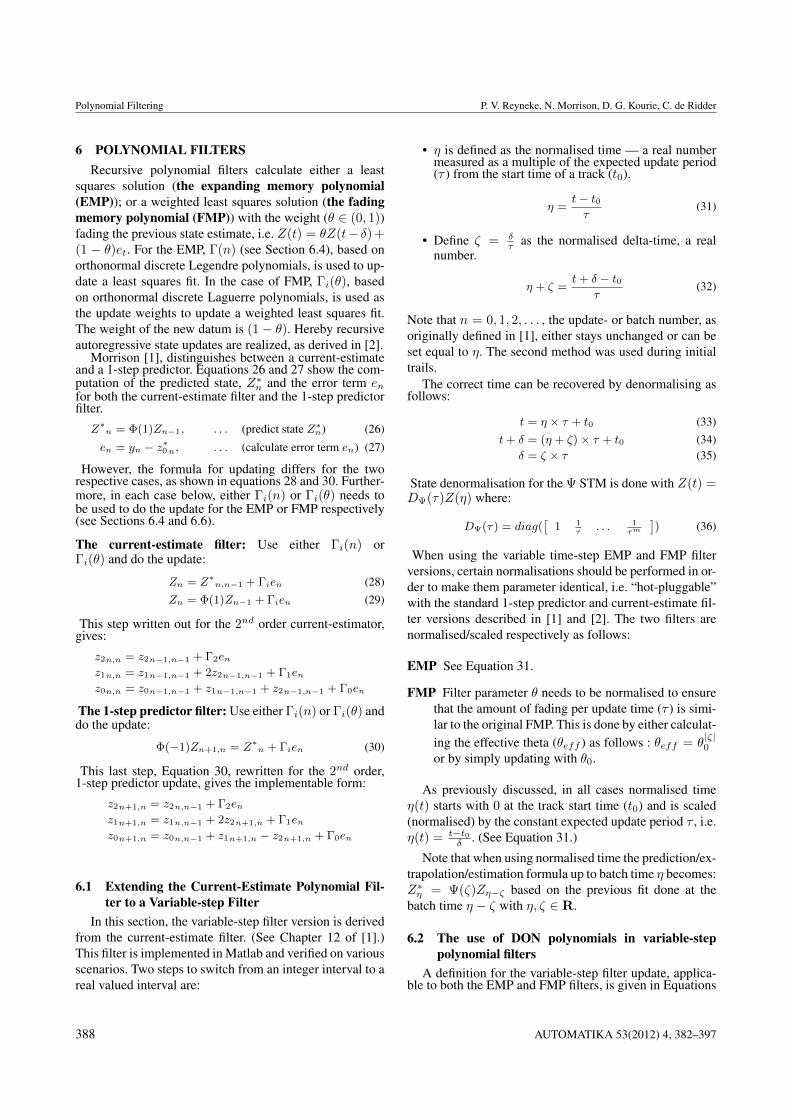
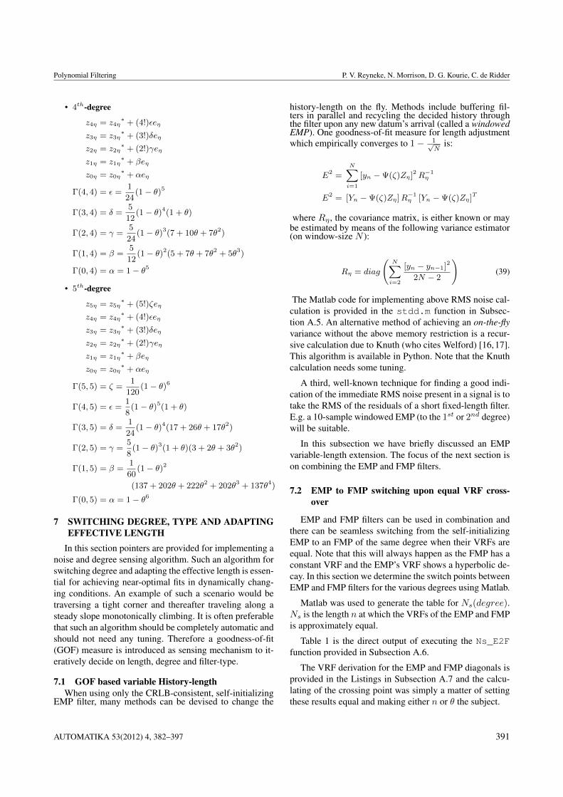
8.2 Results from smoothing very noisy flight data thatverify smoothing and prediction capability

Fig. 2 displays the smoothing achieved on “detectedarea in pixels”, an irregularly detected feature, extractedfrom noisy flight data. The data-set parameters were as fol-lows: PD ≈ 0.25, in the presence of non-linearly changingadditive noise σ as a function of range, and, for an irregularupdate period of around τ = 0.01s.

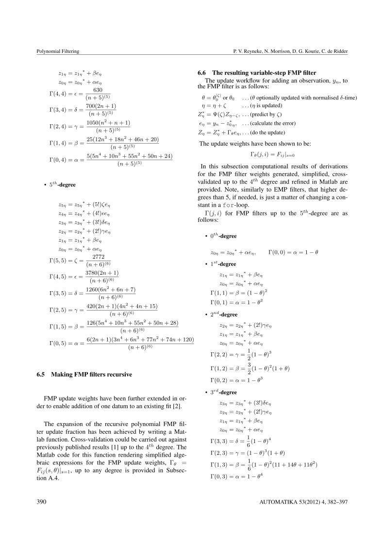
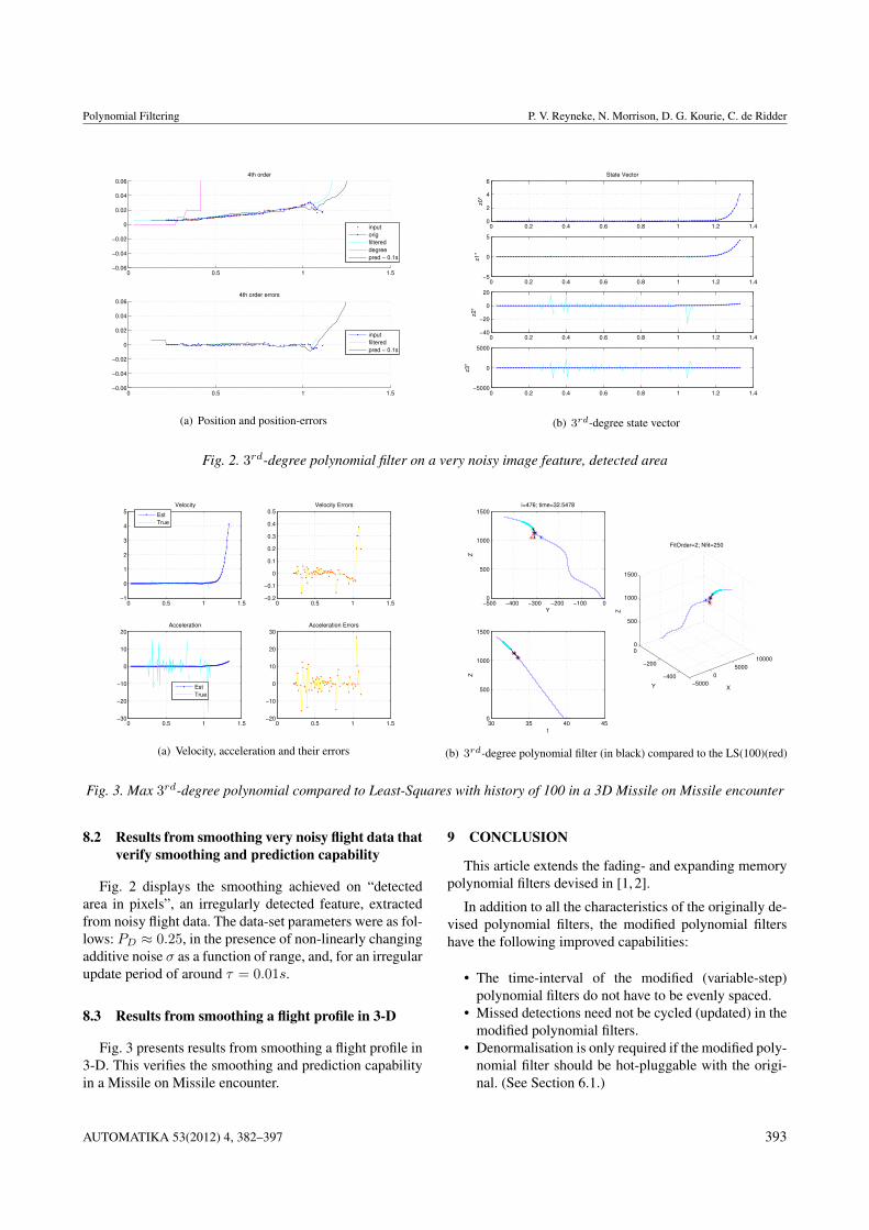
8.3 Results from smoothing a flight profile in 3-D

Fig. 3 presents results from smoothing a flight profile in3-D. This verifies the smoothing and prediction capabilityin a Missile on Missile encounter.

9 CONCLUSION

This article extends the fading- and expanding memorypolynomial filters devised in [1, 2].

In addition to all the characteristics of the originally de-vised polynomial filters, the modified polynomial filtershave the following improved capabilities:

• The time-interval of the modified (variable-step)polynomial filters do not have to be evenly spaced.

• Missed detections need not be cycled (updated) in themodified polynomial filters.

• Denormalisation is only required if the modified poly-nomial filter should be hot-pluggable with the origi-nal. (See Section 6.1.)

AUTOMATIKA 53(2012) 4, 382–397 393


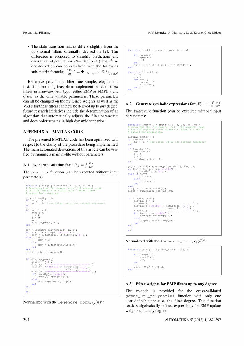
• The state transition matrix differs slightly from thepolynomial filters originally devised in [2]. Thisdifference is proposed to simplify predictions andderivatives of predictions. (See Section 4.) The ith or-der derivation can be calculated with the followingsub-matrix formula: d

iZ(t)dti = Ψ1:N−i,1 × Z(t)1+i:N

Recursive polynomial filters are simple, elegant andfast. It is becoming feasible to implement banks of thesefilters in firmware with type (either EMP or FMP), θ andorder as the only tunable parameters. These parameterscan all be changed on the fly. Since weights as well as theVRFs for these filters can now be derived up to any degree,future research initiatives include the determination of analgorithm that automatically adjusts the filter parametersand does order sensing in high dynamic scenarios.

APPENDIX A MATLAB CODE

The presented MATLAB code has been optimized withrespect to the clarity of the procedure being implemented.The main automated derivations of this article can be veri-fied by running a main m-file without parameters.

A.1 Generate solution for : Pij = 1i!djpdsj

The pmatrix function (can be executed without inputparameters):

function [ dipjs ] = pmatrix( i, j, n, s, ss )% Generates the i^th degree (col) j^th element (row)% for the legendre solution matrix. Note, n and s% passed for uniqueness.

display_pretty = 0;if (nargin < 5)

ss = n+1; % for 1step, ss=n; for current estimatorend

if (nargin < 1)syms s n;i = 4;j = 4;ss = n;display_pretty = 1;

end

pij = legendre_polynomial(j, n, s);if ((i>0) &&(~isa(pij,'double')))

dipj = 1/factorial(i)*diff(pij,'s',i);else if (i>0)

dipj = 0;else

dipj = 1/factorial(i)*pij;end

enddipjs = subs(dipj,s,ss,0);

if (display_pretty)display(['']);display(['------------------------------']);display(['P Matrix (' num2str(i) ', ' ...

num2str(j) ' )']);display(['------------------------------']);if(~isa(dipjs,'double'))

pretty(simple(dipjs));else

display(num2str(dipjs));end

end

end

Normalized with the legendre_norm, cj(n)2:

function [cjn2] = legendre_norm (j, n, s)

if (nargin<1)syms n s;j=4;

endcjn2 = (n+j+1)/(2*j+1)*M(n+j,j)/M(n,j);

end

function [p] = M(z,v)ii=0;p =1;for(i=1:v)

p=p*(z-ii);ii = ii+1;

end;end

A.2 Generate symbolic expressions for: Fij = −1i

i!djfdsj

The fmatrix function (can be executed without inputparameters):

function [ dipjs ] = fmatrix( i, j, The, s , ss )% Generates the i^th degree (col) j^th element (row)% for the leguerre solution matrix. Note, The and s% passed for uniqueness.

display_pretty = 0;if (nargin < 5)

ss = -1; % for 1step, ss=0; for current estimatorend

if (nargin < 1)syms The s;i = 4;j = 4;display_pretty = 1;

end

pij = ((-1)^i)*laguerre_polynomial(j, The, s);if ((i>0) &&(~isa(pij,'double')))

dipj = diff(pij,'s',i);else if (i>0)

dipj = 0;else

dipj = pij;end

enddipjs = dipj/factorial(i);dipjs = subs(dipjs,{s},{ss},0);

if (display_pretty)display(['']);display(['------------------------------']);display(['F Matrix (' num2str(i) ', ' ...

num2str(j) ' )']);display(['------------------------------']);if(~isa(dipjs,'double'))

pretty(simple(dipjs));else

display(num2str(dipjs));end

end

end

Normalized with the laguerre_norm, cj(θ)2:

function [cjn2] = laguerre_norm(j, The, s)

if (nargin<1)syms The s;j=4;

end

cjn2 = The^j/(1-The);end

A.3 Filter weights for EMP filters up to any degree

The m-code is provided for the cross-validatedgamma_EMP_polynomial function with only oneuser definable input n, the filter degree. This functionrenders algebraically refined expressions for EMP updateweights up to any degree.

394 AUTOMATIKA 53(2012) 4, 382–397


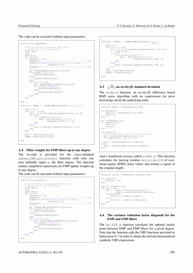
The code can be executed without input parameters:

function all_legendre()

% Run in Matlab to generate EMP filter% weights up to the 5th degreeclear all;clc;syms n s;for (j=0:5)

display([' ']);display(['---------------------------------------']);display(['Expanding Memory filter for degree : ' ...

num2str(j )]);display(['---------------------------------------']);i = j;pj = gamma_EMP_polynomial(i,j,n,s);if(~isa(pj,'double'))

pretty(simple(pj));else

display(num2str(pj));endfor (i=j-1:-1:0)

pj = gamma_EMP_polynomial(i,j,n,s);if(~isa(pj,'double'))


display(num2str(pj));end

endend

end

function [ Gamma ] = gamma_EMP_polynomial( i, j, n, s )

dipj = 0;for (jj = j:-1:0)

pij = ((-1)^jj)*legendre_polynomial(jj, n, s);if (i>0)

if (~isa(pij,'double'))dipj = dipj+diff(pij,'s',i)/...

legendre_norm(jj, n, s);end

elsedipj = dipj+pij/legendre_norm(jj, n, s);

endend

dipj = dipj/factorial(i);Gamma = subs(dipj,s,n,0);

end

A.4 Filter weights for FMP filters up to any degreeThe m-code is provided for the cross-validatedgamma_FMP_polynomial function with only oneuser definable input n, the filter degree. The functionrenders simplified expressions for FMP update weights upto any degree.The code can be executed without input parameters:

function all_laguerre()

% Run in Matlab to generate FMP filter% weights up to the 5th degreeclear all;clc;syms The s;for (j=0:5)

display([' ']);display(['---------------------------------------']);display(['Fading Memory filter for degree : '...

num2str(j )]);display(['---------------------------------------']);i = j;pj = gamma_FMP_polynomial(i,j,The,s);if(~isa(pj,'double'))


display(num2str(pj));endfor (i=j-1:-1:0)

pj = gamma_FMP_polynomial(i,j,The,s);if(~isa(pj,'double'))



endend

end

...function [ Gamma ] = gamma_FMP_polynomial( i, j, ...

The, s )dipj = 0;for (jj = j:-1:0)

pij = ((-1)^i)*(laguerre_polynomial(jj, The, s))...*The^(1*jj);

if (i>0)if (~isa(pij,'double'))

dipj = dipj+diff(pij,'s',i)/...laguerre_norm(jj, The, s);

endelse

dipj = dipj+pij/laguerre_norm(jj, The, s);end

enddipj = dipj/factorial(i);Gamma = subs(dipj,s,0);

end

A.5√Rη , an on-the-fly standard deviation

The stdd.m function, an on-the-fly difference basedRMS noise algorithm with no requirement for priorknowledge about the underlying truth:

function [sout] = stdd(data_in, dim)

if (nargin<1)data_in = randn(1000,1)+[1:1000];dim = 1;

end

sz = size(data_in);if (max(sz)<=1)

sout = 0;return;

end

if nargin==1,% Determine which dimension STDD will usedim = min(find(size(data_in)~=1));if isempty(dim), dim = 1; end

sout = std(diff(data_in))./sqrt(2);else

sout = std(diff(data_in,dim))./sqrt(2);end

And a windowed version, called stddw.m. This functioncalculates the moving window (winsize=20) of root-mean-square (RMS) noise values and returns a signal ofthe original length:

function [sout] = stddw(s_in, winsize, dim)

if (nargin<2)winsize = 20;

end

ida = 1:length(s_in);for (ii = ida)

idx = (ida>=ii-floor(winsize/2))&...(ida<ii-floor(winsize/2)+winsize);

if (nargin<3)sout(ii) = stdd(s_in(idx));

elsesout(ii) = stdd(s_in(idx),dim);

endend

A.6 The variance reduction factor diagonals for theEMP and FMP filters

The Ns_E2F.m function calculates the optimal switchpoint between EMP and FMP filters for a given degree.Note that the function calls the VRF functions provided inSubsection A.7 in order to obtain the relevant denormalisedsymbolic VRF expressions.

AUTOMATIKA 53(2012) 4, 382–397 395


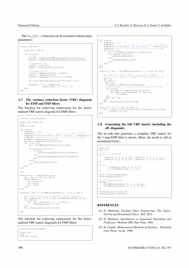
The Ns_E2F.m function can be executed without inputparameters:

function Ns_E2F( )

syms The s tau n;

for (j = 0:5)i = 0;p_Evrf = simple(vrf_EMP_polynomial(i,j,n,s,tau));p_Fvrf = simple(vrf_FMP_polynomial(i,j,The,s,tau));

% assumption onep_Evrf = p_Evrf*n;p_Evrf = limit(p_Evrf,n,Inf)/n;

% assumption twop_Fvrf = expand((p_Fvrf)/(1-The));p_Fvrf = simple(p_Fvrf);p_Fvrf = subs(p_Fvrf,'The',1)*(1-The);

Ns = eval(solve(p_Evrf-p_Fvrf/(1-The),'n'));

display( [' Ns(' num2str(j) ') = ' ...num2str(Ns) '/(1-The)'] );

endend

A.7 The variance reduction factor (VRF) diagonalsfor EMP and FMP filters

The function for achieving expressions for the denor-malised VRF matrix diagonal for EMP filters.

function vrf_diag_emp()

clear all; close allclc;syms n s tau;

for (j=0:5)display([' ']);display(['---------------------------------------']);display(['Expanding Memory VRF for degree : ' num2str(j)]);display(['---------------------------------------']);pjnumi0 = pseries(n+1,j+1,n);pjnumij = pseries(n+j+1,j*2+1,n);for (i=j:-1:0)

pj = vrf_EMP_polynomial(i,j,n,s,tau);

if(~isa(pj,'double'))if (i>0)

pretty(simple(pj*pjnumij)/pjnumij);else

pretty(simple(pj*pjnumi0)/pjnumi0);end

elsedisplay(num2str(pj));

endend

end

end

function [p] = pseries(in,pn,n)pi = in; p = pi; pn = pn-1;while (pn>0)

p = p*(pi-1);pi = pi-1;pn = pn-1;

endend

function [ Sm ] = vrf_EMP_polynomial( i, j, n, s, tau )

ss = n+1; % for 1step, ss=n; for current estimatorSm = pmatrix(i, 0, n, s, ss)^2/legendre_norm(0, n, s);for (k=1:j)

Sm = Sm + pmatrix(i, k, n, s, ss)^2/...legendre_norm(k, n, s);

endSm = (factorial(i)/tau^i)^2*Sm;

end

The function for achieving expressions for the denor-malised VRF matrix diagonals for FMP filters:

function vrf_diag_fmp()

clear all;clc;syms The s tau;

...for (j=0:5)

display([' ']);display(['---------------------------------------']);display(['Fading Memory VRF for degree : ' num2str(j )]);display(['---------------------------------------']);for (i=j:-1:0)

pj = vrf_FMP_polynomial(i,j,The,s,tau);if(~isa(pj,'double'))



endendend

function [ Sm ] = vrf_FMP_polynomial( i, j, The, s, tau )

ss = 1; % for 1step, ss=0; for current estimator% calc row i, start at column j=i and stop at j=j (k)Sm = 0;for (k=i:j)

Am = 0;F_1stepik = fmatrix(i,k,The,s,ss);% calc columm j, start at row j=i, stop at j=j (o)for (o=i:j)

F_1stepio = fmatrix(i,o,The,s,ss);Am = Am + F_1stepik*A(k, o, The, s)*...

F_1stepio;endSm = Sm + Am;

endSm = (factorial(i)/tau^i)^2*Sm;

end

function [ aij ] = A(i, j, The, s)aij = factorial(i+j)/factorial(j)/factorial(i)*(1-The)...

/(1+The)^(i+j+1);end

A.8 Generating the full VRF matrix (including theoff- diagonals)

The m-code that generates a complete VRF matrix forthe 1-step EMP filter is shown. (Here, the result is still innormalised form.)

syms n s;tau = 1;

%% All vrf elementsP = [

pmatrix( 0, 0, n, s, n+1 ) pmatrix( 0, 1, n, s, n+1 )pmatrix( 1, 0, n, s, n+1 ) pmatrix( 1, 1, n, s, n+1 )

];

C2 = [1/legendre_norm( 0, n, s ) 00 1/legendre_norm( 1, n, s )

];

Svrf = P*C2*transpose(P);pretty(simple(Svrf));

%% Vrf Diagonals onlyS_diag = [

vrf_EMP_polynomial( 0, 1, n, s, tau )vrf_EMP_polynomial( 1, 1, n, s, tau )

];

eval(S_diag(1)-Svrf(1,1))eval(S_diag(2)-Svrf(2,2))

REFERENCES

[1] N. Morrison, Tracking Filter Engineering: The Gauss-Newton and Polynomial Filters. IET, 2012.

[2] N. Morrison, Introduction to Sequential Smoothing andPrediction. McGraw-Hill, New York, 1969.

[3] H. Cramér, Mathematical Methods of Statistics. PrincetonUniv. Press, 1st ed., 1946.

396 AUTOMATIKA 53(2012) 4, 382–397


[4] C. R. Rao, “Information and the accuracy attainable in theestimation of statistical parameters,” Bulletin of CalcuttaMathematical Society, vol. 37, 1945.

[5] Z. Long, N. Ruixin, and P. Varshney, “A sensor selection ap-proach for target tracking in sensor networks with quantizedmeasurements,” ICASSP 2008, March 2008.

[6] P. V. Reyneke, N. Morrison, D. Kourie, and C. de Ridder,“Smoothing Irregular data using Polynomial Filters,” Pro-ceedings Elmar-2010, pp. 393–397, 2010.

[7] T. Chihara, An introduction to Orthogonal Polynomials.Gordon and Breach Science Publishers, New York-London-Paris, 1978.

[8] P. Gibbs and S. Gragert, “What is the term used for the thirdderivative of position?,” tech. rep., Usenet Physics FAQ,November 1998.

[9] G. H. Golub and C. F. Van Loan, Matrix Computations.Johns Hopkins University Press, 2nd ed., 1989.

[10] Mathworks, “Matrix exponential function — expm.”http://www.mathworks.com/access/helpdesk/help/techdoc/ref/expm.html, 2009.

[11] C. P. Neuman and D. I. Schonbach, “Discrete (Legendre)orthogonal polynomials - a survey,” International Journalfor Numerical Methods in Engineering, vol. 8, pp. 743–770,Jun 2005.

[12] A. den Brinker and M. Bastiaans, “Modern Signal Trans-formations,” tech. rep., Technishe Universiteit Eindhoven,April 2000.

[13] D. Pollock, A Handbook of Time-Series Analysis, SignalProcessing and Dynamics, pp. 227–291. No. v. 1 in Sig-nal Processing and its Applications, Academic, 1999.

[14] M. F. Aburdene and J. E. Dorband, “On the Computation ofDiscrete Legendre Polynomial Coefficients,” Multidimen-tionsl Systems and Signal Processing, no. 4, pp. 181–186,1993.

[15] E. Brookner, Tracking and Kalman Filtering made Easy.Wiley & Sons, 1st ed., 1998.

[16] D. E. Knuth, The Art of Computer Programming: Seminu-merical Algorithms, vol. 2, p. 232. Addison-Wesley,Boston, 3 ed., 1998.

[17] B. P. Welford, “A note on a Method for Calculating Cor-rected Sums of Squares and Products,” Technometrics,vol. 4, no. 3, pp. 419–420, 1962.

Pieter V. Reyneke a masters student at the De-partment of Computer Science, University ofPretoria (UP), completed a BSc in Electronic En-gineering at UP in 1991. He is currently practic-ing as a Algorithm Engineer at Denel Dynamics,SA.

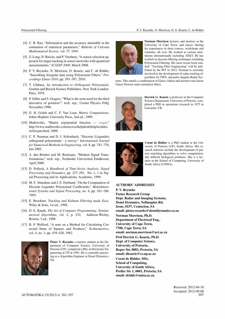
Norman Morrison lectures and mentors at theUniversity of Cape Town, and enjoys sharinghis experiences in short courses, workshops andseminars, all over. He worked at various insti-tutions internationally including AT&T. He hasworked on discrete filtering techniques includingPolynomial Filtering. His most recent book enti-tled: “Tracking Filter Engineering” will be pub-lished by the IET in 2012. Norman is currentlyinvolved in the development of radar tracking al-gorithms for TWS- and pulse-doppler Radar Sys-

tems. This entails a combination of Gauss-Aitken and iterative non-linearGauss-Newton state-estimation filters.

Derrick G. Kourie a professor in the ComputerScience Department, University of Pretoria, com-pleted a PhD in operations research in 1975 atLancaster, UK.

Corné de Ridder is a PhD student at the Uni-versity of Pretoria (UP), South Africa. Her re-search interests include the development of pat-tern matching algorithms to solve computation-ally difficult biological problems. She is a lec-turer at the School of Computing, University ofSouth Africa (UNISA).

AUTHORS’ ADDRESSESP. V. ReynekeFastar Research GroupDept. Radar and Imaging Systems,Denel Dynamics, Nellmapius Rd,Irene, 0157, Centurion, SAemail: [email protected] Morrison, Ph.D.Department of Electrical Eng.,University of Cape Town,7700, Cape Town, SAemail: [email protected] Derrick G. Kourie, Ph.D.Dept. of Computer Science,University of Pretoria,Roper Str, 0002, Pretoria, SAemail: [email protected]é de Ridder, MSc.School of Computing,University of South Africa,Preller Str 1, 0001, Pretoria, SAemail: [email protected]

Received: 2012-04-10Accepted: 2012-09-08

AUTOMATIKA 53(2012) 4, 382–397 397

polynomial filtering: to any degree on irregularly sampled data

Documents