planning high order trajectories with general initial … high order trajectories with general...
TRANSCRIPT
Planning High Order Trajectories with General Initial and
Final Conditions and Asymmetric Bounds
Ben Ezair1,3 Tamir Tassa1 Zvi Shiller2∗†‡
Abstract
This paper presents a trajectory planning algorithm for linear multi-axis systems.It generates smooth trajectories of any order subject to general initial and final con-ditions, and constant state and control constraints. The algorithm is recursive, as itconstructs a high order trajectory using lower order trajectories. Multi-axis trajecto-ries are computed by synchronizing independent single-axis trajectories to reach theirrespective targets at the same time.
The algorithm’s efficiency and ability to handle general initial and final conditionsmake it suitable for reactive real time applications. Its ability to generate high ordertrajectories makes it suitable for applications requiring high trajectory smoothness. Thealgorithm is demonstrated in several examples for single- and two-axis trajectories oforders 2− 6.
1 Introduction
This paper addresses the problem of planning time-efficient trajectories for linear multi-axissystems with arbitrary initial and final states, subject to constant constraints on any numberof trajectory derivatives. In the context of robot motion, the trajectory planning problemconsists of generating a smooth trajectory that connects given initial and final conditions,is optimal with respect to some cost function, and satisfies given bounds on a number ofits time derivatives. The number of derivatives considered, also called the trajectory order,usually reflects the order of the robot dynamic model, whereas the bounds on the timederivatives reflect state and control constraints of the robot system.
Pre-computed feasible trajectories can be used to accurately guide a dynamic systemto the destination state by serving as the desired inputs to the system’s joint controllers.A carefully selected trajectory can prevent the joint controllers from reaching saturation, acommon cause for tracking errors. In addition, they are essential when coordinated motionof several joints is desired. When used in a feed-forward fashion, they can significantlyreduce tracking errors by reducing the magnitude of the tracking error needed to drive thesystem along the trajectory [22].
∗1Ben Ezair and Tamir Tassa are with The Department of Mathematics and Computer Science, TheOpen University, Israel. ben [email protected] & [email protected]
†2Zvi Shiller is with the Department of Mechanical Engineering and Mechatronics, Ariel [email protected]
‡3The research of the first author was partially supported by The Open University of Israel’s ResearchFund (grant no. 32046).
1

High order trajectories are needed to account for actual and unmodeled system dy-namics. Unmodeled dynamics may arise from unmodeled actuators and drivers, and fromunmodeled flexible modes. For both cases, high order smooth trajectories are desired. Inthe case of unmodeled actuator and driver dynamics, a smooth trajectory may be easier tofollow when using it as a control input, since it may not demand a response that is beyondthe capabilities of the actuator/driver system. For example, using a third order trajectoryto drive a DC motor assumes that the motor voltage serves as the control input. Hence,by choosing a third order trajectory in this context it is assumed that the motor can reactinstantaneously to abrupt switches in the voltage signal. In practice, however, the drivermay not be able to generate instantaneous voltage changes, thus causing some delay in thesystem response, or even completely ignoring (filtering) particularly short voltage pulses.Such delays and inaccuracies are the cause of tracking errors. Tracking errors could beavoided if the trajectory was of a higher order, for which the third derivative, and hence thevoltage signal, is smooth. A further discussion of the benefits of higher order trajectories,including experimentation, can be found in [16, 13].
In the case of a flexible system, a high order smooth trajectory may not excite highfrequency flexible modes, thus resulting in slower, yet vibration-free motion. It should benoted that the clear benefits of high order smooth trajectories come at the cost of slowermotion. The appropriate balance between motion time and smoothness should be set inaccord with the characteristics of the application at hand. Some applications may demandextreme accuracy and, hence, should use a high order trajectory; in other applications, afast second or third order trajectory may suffice. One of the advantages of our algorithm isthat this choice can be easily made by specifying the desired trajectory order.
One challenge in trajectory planning is to generate a high order smooth trajectory onthe fly, during motion, to account for the current motion state and to respond to eventsthat are identified during motion [11]. This, in turn, requires the algorithm to be highlyefficient and to be able to accept arbitrary initial and final conditions.
The algorithm proposed herein generates time-efficient trajectories between arbitraryinitial and final states for a linear system of any given order, subject to constant andasymmetric state and control constraints. Given the motion constraints, the algorithmgenerates a feasible trajectory while attempting to minimize motion time. The algorithm isrecursive, in the sense that it reduces the original problem of order m to smaller problems oforder m−1. The recursion is based on a binary search, which contributes to the algorithm’scomputational efficiency. Multi-axis trajectories are computed by synchronizing single-axistrajectories to reach their respective targets at the same time.
1.1 Related work
Early work on trajectory planning of multi-axis systems was based on decomposing the prob-lem into path planning and trajectory planning. It consists of first generating a feasible path,then computing the time optimal velocity profile along the specified path [2, 18, 24, 25, 26],and finally modifying the path to obtain the time optimal trajectory [1, 23]. The optimalvelocity profile is computed by switching between the maximum and minimum allowed ac-celeration values along the path, for a second order system [2]. Adding velocity constraintsresults in a bang-zero-bang structure of the acceleration profile [21]. The optimization along
2
a specified path was extended to account for non-linear third order systems, subject to gen-eral jerk constraints [28]. While this approach allowed solving difficult multi-axis problemswith non-linear second or (at most) third order dynamics and any obstacle constraints, it isoff-line in nature. Higher order dynamics are often needed to produce smooth trajectoriesthat account for high order actuator dynamics and high order vibration modes. Computingsmooth high order trajectories poses a special challenge in online motion planning, namely,applications where the trajectory is updated “on the fly” to account for tracking errorsand changes in the environments. There are several different approaches used by morerecent works for generating smooth trajectories. One approach uses polynomials or otherfunctions to approximate the desired trajectories, often optimizing a parametric curve inorder to achieve near optimal results [15, 17, 19]. Piazzi and Visioli [19] optimize cubicsplines to minimize jerk for a specified motion time. Petrinec and Kovacic [17] use fourthand fifth order polynomials and various heuristics to produce smooth multi-axis trajecto-ries. Macfarlane and Croft [15] compute trajectories that are represented by fifth orderpolynomials.
Another approach for trajectory generation relies on Pontryagin’s maximum principle[20], which for time optimal control for linear systems with state constrains suggests a bang-zero-bang structure for the control input. Hence, the sought after trajectory is divided intosegments, where the value of the highest derivative is constant in each segment, equalingits upper or lower bounds, or zero.
Liu [14] presents an algorithm that produces a third order trajectory that is constructedby dividing the trajectory to seven segments. They limit the trajectory to be one of severalforms that are possible for a seven segment trajectory. This allows them to reduce theproblem to two steps: first identifying the best form out of a finite set, then solve theequations for that form to calculate the exact trajectory. This basic approach can beextended to produce multi-axis trajectories by synchronizing several single-axis trajectories[9, 3, 10]. They use a similar method for each individual axis but also lower the derivativebounds of faster axes in order to synchronize them with the slower ones.
Haschke et al. [8] also produce a multi-axis third order trajectory based on a sevensegment approach. They emphasize the online capabilities of their algorithm that is designedto produce a third order halting trajectory. The main tool used here is a manipulation of theacceleration profile to slow the trajectory. This allows slowing down single-axis trajectoriesso that they comply with the derivative bounds, and not overshoot the target position; itcan also be used to synchronize them with slower axes. Works by Kroger et al. [11, 12]also focus on online algorithms for second and third order trajectories, using a thoroughanalysis of possible acceleration profiles to handle more general initial and final conditions.These works in many ways formalize the steps used by other algorithms. The first step ofidentifying the general form of the trajectory is accomplished through the use of decisiontrees that map out all possible forms for the requested trajectory. Each of the possibleforms can then be used to define a system of equations, that is solved to get all possiblesolutions, amongst which the optimal solution can be found. This also allows a morethorough approach to be used to synchronize multiple axes: since all possible solutions foreach axis are known, the best motion time to synchronize all axes can be easily identified.
Lambrechts et al. [13] produce fourth order trajectories. Here too the basic idea isdividing the trajectory into segments where the highest derivative has one of three constant
3

values. A fourth order trajectory, however, requires more segments than a third ordertrajectory, and is much more complex. They solve this by limiting themselves to dealingwith rest to rest motion, and assuming a single specific trajectory form. This form has eightsegments with a non-zero snap (the fourth derivative of position), and all of these segmentshave the exact same time length. By progressively reducing the length of these segments,so that they comply with the motion derivative limits and the target position, they thencalculate the desired fourth order trajectory. Nguyen et.al. [16] developed an algorithm thatgenerates trajectories of arbitrary order with zero initial and final conditions and symmetricstate and control constraints. It is based on dividing the trajectory into a recursive structureof S-curve segments. This recursive structure is used to construct an algorithm that is ageneralization to an arbitrary order of the fourth order trajectory generation algorithmdescribed in [13]. The use of recursive S-curves forms is also the basis for the algorithmwhich we present herein.
1.2 Our algorithm
This paper presents a novel algorithm for planning trajectories for linear systems of anyorder between arbitrary initial and final states (position and its time derivatives), subjectto given constant state and control constraints; the algorithm is geared towards minimizingmotion time. The generality of our approach makes the algorithm suitable for both onlineand offline trajectory planning. The algorithm is recursive, as it reduces the original problemof order m to problems of order m − 1, until it reaches basic problems that can be solveddirectly. The algorithm is modular, as it may accept any external solver for the basictrajectory generation problem which is solved directly in order to terminate the recursion.(Here, we offer to stop the recursion at order m = 2, for which a simple analytical solutionexists. However, it can also continue until m = 1, for which the basic solution is trivial, oruntil any other order for which a direct and efficient solution exists or will become available.)
The algorithm is efficient, as demonstrated in several experiments (see Table 2 in Sec-tion 2.3). Finally, the basic algorithm is extended to generate multi-axis trajectories bysynchronizing independent single-axis trajectories to reach their respective targets at thesame time.
Table 1 compares our algorithm with the leading comparable algorithms that considersimilar settings as ours; i.e., algorithms that deal with linear systems subject to constantconstraints and attempt to minimize motion time. (All of those algorithms were reviewedin Section 1.1.)
All of the comparable algorithms are limited either in the order of the trajectoriesthat they may produce, or in the initial and final conditions that they may accept. Ouralgorithm’s main advantage is its generality and flexibility, as it is applicable to a widerrange of scenarios than the other algorithms.
It should be noted that algorithms for non-linear systems exist, e.g. [5, 7, 28], however,they are limited (at least for now) to order m ≤ 3, use other cost functions, or are limitedto a specified path (usually using an arc length parametrization). Algorithms treatingnon-linear systems, which are typically computationally intensive, may not be suitable formulti-axis non-linear systems that need to react on-line to fast changing environments.One approach to handling such cases is to approximate the non-linear system with a linear
4

model, and then use an efficient on-line trajectory generator. The resulting trajectory maynot be optimal, but it would be smooth, of the desired order, not constrained to a specifiedpath, and satisfying approximate (constant) state and control constraints. So, in effect,linear trajectory generators may be useful for both linear and non-linear systems. It is inthis context that we propose our algorithm as a contribution to the existing class of ”linear”trajectory generators.
Ref. Order Initial & Final Conditions Constraints Online Optimal
[11] 2 general symmetric yes yes[3] 3 zero acceleration symmetric yes yes[8] 3 ends at rest symmetric yes yes[12] 3 zero final acceleration symmetric yes yes[13] 4 rest to rest symmetric no no[16] any rest to rest symmetric no noOurs any general asymmetric yes no
Table 1: Comparison of trajectory generation algorithms
2 Single-axis trajectories
We wish to compute a pair ⟨T, x(t)⟩, where x(t) denotes the position of a moving objectalong a given axis, such that (a) x(t) satisfies given initial and final conditions at t = 0 andt = T ,
x(0) = x0s , x(i)(0) = xis , 1 ≤ i ≤ m− 1 , (1)
x(T ) = x0f , x(i)(T ) = xif , 1 ≤ i ≤ m− 1 , (2)
where x(i)(t), i ≥ 1, is the i-th order derivative of x(t); (b) it is constrained by constantlower and upper bounds,
ximin < 0 < ximax , 1 ≤ i ≤ m (3)
ximin ≤ x(i)(t) ≤ ximax , t ∈ [0, T ] , 1 ≤ i ≤ m ; (4)
and (c) the time T =∫ T0 1dt is minimized. The number m ≥ 1 of constrained derivatives is
called the order of the problem. A pair ⟨T, x(t)⟩ that satisfies the initial and final conditions,(1)–(2), and the lower and upper bounds (4) is called a feasible solution. A solution isoptimal if is feasible and minimizes T .
This single-axis trajectory planning problem may be viewed as a time optimal controlproblem of a linear system of ordinary differential equations with m state variables (beingthe position function x(t) and its first m−1 derivatives) and a single control variable (beingthe m-th derivative x(m)(t)), subject to initial and final conditions and state and controlconstraints. The structure of the optimal control for such problems can be shown to havea bang-zero-bang structure [4].
The solution for the case m = 1 is trivial, consisting of a constant velocity motion.A solution for m = 2 is given in [11]. Our approach in solving higher order problems isrecursive, as it reduces a problem of order m to problems of order m− 1, repeatedly, untilm = 2, in which case the problem can be solved directly.
5

2.1 A single-axis trajectory planning algorithm
2.1.1 Overview
The algorithm for computing high order trajectories is motivated by the observation thatintegrating a bang-zero-bang control profile yields an S-curve structure (see Figure 1 forthe case m = 3). A typical S-curve can be divided into three segments: (I) accelerationfrom the initial state; (II) cruising at a constant velocity; and (III) deceleration to the finalstate. This structure, repeats recursively since the velocity profile, as well as the profiles ofhigher derivatives, consist of two or more S-curve segments.
0
500
1000
0
1000
2000
−2
0
2x 10
4
0 0.2 0.4 0.6−2
0
2x 10
5
x
x(1)
x(2)
x(3)
t
III
I II III
III
Figure 1: The recursive structure of the trajectory
The recursive algorithm looks for a solution with an S-curve position profile. Themain loop attempts to find the best value for the constant velocity in segment II. Given acandidate value v for that velocity, the algorithm computes the velocity profile in segmentsI and III by invoking recursion. Specifically, it solves in each of those segments a reducedorder trajectory planning problem for the velocity profiles. Once the velocity profiles inall three segments are found, the algorithm checks that the corresponding position profileis a feasible solution. When the resulting solution is non-feasible, the algorithm reduces|v|; when the resulting solution is feasible, the algorithm increases |v| in order to reducemotion time. The algorithm terminates when the optimal value of v is found within somepredetermined accuracy, and it outputs the found position profile x(t).
2.1.2 Detailed description
We proceed to describe the operation of Algorithm 1 that implements the above procedure.The algorithm accepts as inputs the problem order, the initial and final conditions, and thelower and upper constraints. It outputs a feasible solution ⟨T, x(t)⟩ which is time-efficientand in some cases optimal.
If m = 2 the algorithm outputs the analytic solution (Step 1). Otherwise, we set ∆x tobe the distance to be traveled (Step 2) and start a binary search for v within the allowedrange of values [x1min, x
1max]. The variables vmin and vmax hold the lower and upper limits
of the search range; they are initialized in Step 3. The variable v holds the last value of v
6

that produced a feasible solution. It is initialized to an illegal value (x1max + 1) in Step 3,and so is v.
During the binary search (Steps 4-18), we consider the midpoint of the current range asthe candidate value for v (Step 6). Given a candidate value for v, the trajectory planningproblem in the acceleration and deceleration segments (I and III) are well defined and canbe solved by invoking recursion. Let v1(t) be the velocity profile in segment I, from theinitial value x1s to the cruising velocity v, and let τ1,v denote the duration of that segment.Then in Step 7 we compute ⟨τ1,v, v1(t)⟩ by solving a problem of order m− 1 for x′(t) alongthat segment. The initial conditions for that reduced order problem are (x1s, . . . , x
m−1s );
its final conditions are (v, 0, . . . , 0) (since we wish to reach the velocity v with all higherderivatives zero); and the lower and upper bounds on the derivatives are in accord withthose of the original problem. Similarly, we invoke recursion in Step 8 to compute v3(t), thevelocity profile in segment III, from v to the final value x1f , and the corresponding durationτ3,v.
Next, we compute the distance covered in segments I and III, ∆x1 and ∆x3 (Step 9). ∆is the remaining distance that needs to be traveled in the intermediate segment II in order tocomplete a journey of length ∆x. Since the velocity along segment II is constant and equalsv, the duration of that segment should be τ2,v = ∆/v (Step 10). If τ2,v is nonnegative, thenthis tested value of v leads to a valid trajectory; in that case we record that value of v inthe variable v (Step 11).
The search ends once the lower and upper limits of the search are sufficiently close (Steps12-14). In that case, we set v, vmin and vmax to be the last value of v that produced a validsolution. If v still equals its initial value x1max + 1 (a forbidden value for v, as it is outsidethe allowed range [x1min, x
1max]), then the search failed to find a valid v. This may occur if
the problem parameters define a range of legitimate v values that is smaller than ε, and,consequently, cannot be captured using a binary search with such accuracy. (We note thatinstead of using the same value of ε for all levels, we may define for each level i, 1 ≤ i ≤ m,a different value εi.) Otherwise, if v is a legal value, then the algorithm performs anotheriteration. Since v, vmin, and vmax equal the last valid value of v, the subsequent setting oflast v and v in Steps 5-6 will cause the algorithm to perform the next iteration with v = vand then terminate the loop when it examines the termination condition in Step 18.
In case the lower and upper limits of the search are still far apart, we check the valueof ∆ to determine how to proceed with the search: if ∆ > 0, then we examine profiles withhigher values of v (Step 15); if ∆ < 0, we consider lower values of v (Step 16); if ∆ = 0,we terminate the search by setting last v to equal v (Steps 17). The search ends whenlast v = v. After determining the value v, we compute T and construct the profile of x′
as the concatenation of three segments – v1(t), v,v3(t) (Steps 19-20). Finally, we integratex′(t) to obtain x(t) (Step 21).
2.1.3 A note on optimality
Algorithm 1 uses a simple greedy approach in the search of a solution with a minimal motiontime. The solution is optimal for rest-to-rest motions of order m ≤ 3. The proof of thisclaim and further discussion can be found in Appendix A. Although Algorithm 1 attemptsto minimize motion time, the solution is not necessarily optimal, because the algorithm is
7
based on two assumptions that are not always satisfied:(A1) The duration of segment II is a continuous and monotonic function of v.(A2) The velocity during segment II is constant, implying that during this phase all
higher derivatives are zero.The first assumption affects the way the algorithm updates v (steps 15-16). If this
assumption is not satisfied, the algorithm may choose a value of v that will result in anon-optimal motion time. The second assumption is more central to Algorithm 1, as itallows us to subdivide the trajectory into two S curves that can be joined together witha simple constant velocity motion. However, this assumption is not always true, e.g. incases where the optimal trajectory either always accelerates or always decelerates. In suchcases, the algorithm would return a solution that is of a different structure than that of theoptimal trajectory. Both assumptions make the algorithm efficient by limiting the numberof possible trajectory forms we need to consider. This, in turn, greatly simplifies the searchfor segment II that connects segments I and III.
2.2 Complexity
The main computational effort in Algorithm 1 is the binary search, performed in steps 4-18,for the optimal value of v in the interval [x1min, x
1max]. All other operations performed by
the algorithm (including the solutions for m = 1 and m = 2) take constant time. Sincethe binary search terminates when the interval size becomes smaller than or equal to ε1,
it executes at most log2x1max−x1
minε1
iterations. In each of those iterations, the algorithminvokes two recursive calls for solving problems of order m − 1; in addition, it performsthe computations in Steps 9-17. The time complexity of the latter computations can bebounded by a constant. If this constant is denoted d, and the time for solving the problemof order m is denoted Tm, then:
Tm =
(log2
x1max − x1min
ε1
)· (2Tm−1 + d) . (5)
This search repeats for each level i in the recursion in the range [ximin, ximax]; it terminates
when the interval size becomes smaller than or equal to εi. Solving the recursive equation(5) yields Tm in terms of T2, d, the interval lengths (ximax − ximin), and εi:
Tm = T2 ·m−2∏i=1
(2Ci) + d ·
m−2∑j=1
(2j−1
j∏i=1
Ci
) , (6)
where
Ci = log2ximax − ximin
εi, (7)
Let C = max1≤i≤m−2Ci. Then, by Eq. (6):
Tm ≤ T2 · (2C)m−2 + dC ·
m−2∑j=1
(2C)j−1
= T2 · (2C)m−2 + dC · (2C)m−2 − 1
2C − 1.
8

As C > 1 for any reasonable setting of εi, we conclude that
Tm ≤ (2C)m−2 ·
(T2 +
dC
2C − 1
)≤ (2C)m−2(T2 + d) .
Thus
Tm ≤(2 max1≤i≤m−2
log2ximax − ximin
εi
)m−2
(T2 + d) . (8)
The total time taken by the algorithm is determined by the range of values that haveto be searched at each level ximax − ximin, the desired accuracy in that level εi, and theproblem order m. The more accurate is the search (lower εi), the longer is the computationtime. Similarly, the larger is the range, the longer is the search. However, since this is abinary search, the overall dependence on these factors is only logarithmic. In contrast, thedependence of the runtime on m is exponential. However, as m denotes the order of theproblem, its value in practical applications is typically very small (note that most studiesthus far concentrated on m ≤ 3 and only few studies considered orders up to m = 5). Forsuch values of m, and even higher ones, the algorithm is still computationally practical, asdemonstrated by our experimentation in the next section.
2.3 Experiments: Single-axis trajectories
Algorithm 1 was implemented in C++ and was executed as a normal priority process onan Intel Pentium D 3.0 GHz processor, using a normal Microsoft windows XP system. Wetested the algorithm for high order trajectories (with orders up to m = 7) with zero andnon-zero initial and final conditions. The bounds used for the motion derivatives in theseexamples were chosen high (and low) so that motion derivatives reach their maximal (andminimal) values. Tight bounds on the high derivatives might result in frequent switches ofthe highest derivative, which might not let the lower derivatives reach (and sustain) theirextreme values.
Figure 2 shows trajectories computed by the algorithm for various values of m, ∆x = 50,zero initial and final conditions (xis = xif = 0, 1 ≤ i ≤ m− 1); the state constraints in this
example were |x(i)| ≤ 102+i. These results show that motion time and smoothness increasewith the trajectory order, because of the added limits on higher derivatives. The m = 2profile in Figure 2 is the fastest, but it is not smooth as already its acceleration profileis discontinuous. The m = 6 profile, on the other hand, is the slowest, but it exhibitsdiscontinuities only in its sixth derivative.
Figure 3 shows a solution for the same setting as in Figure 2, for m = 4, except that theinitial and final conditions on the velocity are nonzero: x1s = 70 and x1f = 60. All of thesesolutions share the familiar bang-zero-bang pattern.
Figure 4 shows an asymmetric third order trajectory that was computed by our al-gorithm. For this trajectory we used ∆x = 50, and zero initial and final conditions(xis = xif = 0, 1 ≤ i ≤ m − 1); the derivative constraints were −1000 ≤ x(1) ≤ 200,
−10000 ≤ x(2) ≤ 2000, and −100000 ≤ x(3) ≤ 20000. The capability of our algorithm tosupport asymmetric constraints may be useful in situations where such asymmetry is part
9

of the system dynamics: e.g., in a standard car where acceleration is created by a motor,while deceleration is achieved through the use of a mechanical brake.
Figure 5 shows another trajectory computed by the algorithm. For this fourth ordertrajectory we used ∆x = 20, and zero initial and final conditions (xis = xif = 0, 1 ≤ i ≤m − 1). The derivative constraints for this case were: −10 ≤ x(1) ≤ 10, −1 ≤ x(2) ≤ 1,−10 ≤ x(3) ≤ 10, and −10 ≤ x(4) ≤ 10. Using tight bounds on the high derivatives resultedin most derivatives not reaching their extreme values, except the acceleration for which thebounds were particularly tight.
0 0.5 10
10
20
30
40
50
t
x
m=2m=3m=4m=5m=6
0 0.5 10
200
400
600
800
t
x(1)
m=2m=3m=4m=5m=6
Figure 2: Trajectory position (left) and velocity (right) for m = 2, 3, 4, 5, 6
0 0.1 0.2 0.3 0.40
20
40
60
t
x
0 0.1 0.2 0.3 0.450
100
150
200
250
t
x(1)
Figure 3: Fourth order trajectory position (left) and velocity (right) with nonzero initialand final conditions
Table 2 shows the average runtimes of Algorithm 1 for various values ofm, when executedwith the same inputs as used to generate the trajectories in Figure 2. The parameter εi
was set so that the accuracy is 0.01%, i.e.,ximax−xi
minεi
= 0.0001 for all i. For each m, theaverage runtime was computed by averaging several runs of the algorithm.
As can be seen in Table 2, the runtime changes exponentially with respect to m, asdiscussed in Section 2.2. However, as m is typically a small integer, the algorithm remainscomputationally practical. In particular, the runtimes form ≤ 5 are practical for both offlineand online applications. The runtime for m = 6 might call for code optimization in order tobe practical for online applications, but it is certainly practical for offline applications. The
10

0 0.05 0.1 0.15 0.2 0.25 0.3 0.35 0.4 0.450
10
20
30
40
50
60
t
x
0 0.05 0.1 0.15 0.2 0.25 0.3 0.35 0.4 0.450
20
40
60
80
100
120
140
160
180
200
x(1)
t
0 0.05 0.1 0.15 0.2 0.25 0.3 0.35 0.4 0.45−3000
−2000
−1000
0
1000
2000
3000
x(2)
t0 0.05 0.1 0.15 0.2 0.25 0.3 0.35 0.4 0.45
−12
−10
−8
−6
−4
−2
0
2
4x 10
4
x(3)
t
Figure 4: A third order trajectory with asymmetric bounds (position and all derivatives).
runtime for m = 7 (an order which seems currently to be beyond the need of any practicalapplication) renders the algorithm still practical for offline applications.
We note that Algorithm 1 may be parallelized, as Steps 7 and 8 are independent of eachother and could be executed in parallel. It is therefore possible to reduce the runtime by afactor of up to 2m−2 on a multi-core CPU, depending on the number of processes that canbe executed in parallel.
Order Number of runs Average runtime [s]
3 1000 0.0000744 1000 0.0021415 10 0.06256 10 1.95157 10 80.064
Table 2: Runtimes (seconds) for several profile orders
3 Multi-axis trajectories
The single-axis trajectory planning algorithm can be used for solving multi-axis trajectoryplanning problems. We wish to compute a pair ⟨T, (x1(t), . . . , xn(t))⟩, where (x1(t), . . . , xn(t))is a function that connects two points in the Euclidean space Rn in minimal time, subjectto the following constraints: (a) xj(t) satisfies given initial and final conditions at t = 0 and
11

0 2 4 6 8 100
5
10
15
20
25
t
x
0 2 4 6 8 100
0.5
1
1.5
2
2.5
3
3.5
4
4.5
x(1)
t
0 2 4 6 8 10
−1
−0.5
0
0.5
1
x(2)
t0 2 4 6 8 10
−4
−3
−2
−1
0
1
2
3
4
x(3)
t
0 2 4 6 8 10
−10
−8
−6
−4
−2
0
2
4
6
8
10
x(4)
t
Figure 5: A fourth order trajectory with low bounds for the higher derivatives (positionand all derivatives).
t = T ,
xj(0) = xj,0s , x(i)j (0) = xj,is , (9)
xj(T ) = xj,0f , x(i)j (T ) = xj,if , (10)
where 1 ≤ i ≤ m−1 and 1 ≤ j ≤ n (hereinafter the index j denotes the axis while i denotesthe derivative order); (b) it is constrained by constant lower and upper bounds,
xj,imin ≤ x(i)j (t) ≤ xj,imax , t ∈ [0, T ] , (11)
where 1 ≤ i ≤ m and 1 ≤ j ≤ n; and (c) the time T =∫ T0 1dt is minimized.
To solve the multi-axis trajectory planning problem, we begin by first solving the nindependent single-axis problems. For each axis 1 ≤ j ≤ n, we get a single-axis trajectory,xj(t), that satisfies the initial and final conditions and kinematic bounds along that axis,
12
0 0.5 1 1.5 20
0.2
0.4
0.6
0.8
1
t
x
m=2m=3m=4m=5m=6
0 0.5 1 1.5 2−0.5
0
0.5
1
1.5
t
x(1)
m=2m=3m=4m=5m=6
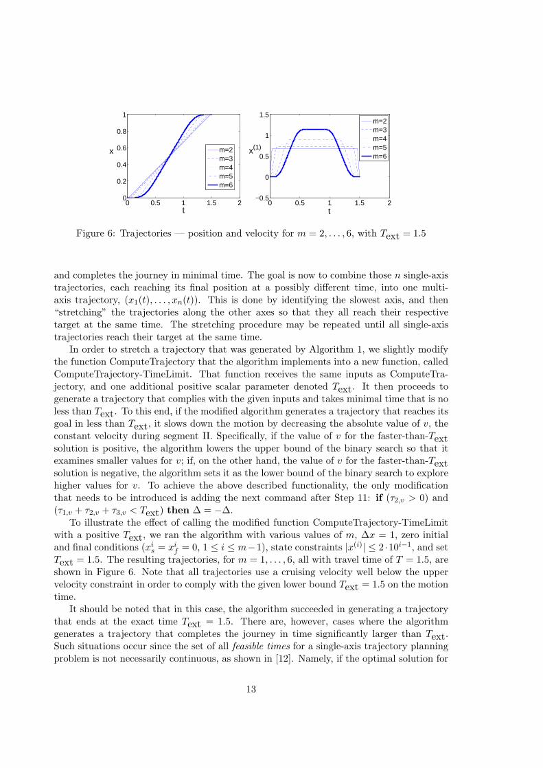
Figure 6: Trajectories — position and velocity for m = 2, . . . , 6, with Text = 1.5
and completes the journey in minimal time. The goal is now to combine those n single-axistrajectories, each reaching its final position at a possibly different time, into one multi-axis trajectory, (x1(t), . . . , xn(t)). This is done by identifying the slowest axis, and then“stretching” the trajectories along the other axes so that they all reach their respectivetarget at the same time. The stretching procedure may be repeated until all single-axistrajectories reach their target at the same time.
In order to stretch a trajectory that was generated by Algorithm 1, we slightly modifythe function ComputeTrajectory that the algorithm implements into a new function, calledComputeTrajectory-TimeLimit. That function receives the same inputs as ComputeTra-jectory, and one additional positive scalar parameter denoted Text. It then proceeds togenerate a trajectory that complies with the given inputs and takes minimal time that is noless than Text. To this end, if the modified algorithm generates a trajectory that reaches itsgoal in less than Text, it slows down the motion by decreasing the absolute value of v, theconstant velocity during segment II. Specifically, if the value of v for the faster-than-Textsolution is positive, the algorithm lowers the upper bound of the binary search so that itexamines smaller values for v; if, on the other hand, the value of v for the faster-than-Textsolution is negative, the algorithm sets it as the lower bound of the binary search to explorehigher values for v. To achieve the above described functionality, the only modificationthat needs to be introduced is adding the next command after Step 11: if (τ2,v > 0) and(τ1,v + τ2,v + τ3,v < Text) then ∆ = −∆.
To illustrate the effect of calling the modified function ComputeTrajectory-TimeLimitwith a positive Text, we ran the algorithm with various values of m, ∆x = 1, zero initialand final conditions (xis = xif = 0, 1 ≤ i ≤ m−1), state constraints |x(i)| ≤ 2 ·10i−1, and setText = 1.5. The resulting trajectories, for m = 1, . . . , 6, all with travel time of T = 1.5, areshown in Figure 6. Note that all trajectories use a cruising velocity well below the uppervelocity constraint in order to comply with the given lower bound Text = 1.5 on the motiontime.
It should be noted that in this case, the algorithm succeeded in generating a trajectorythat ends at the exact time Text = 1.5. There are, however, cases where the algorithmgenerates a trajectory that completes the journey in time significantly larger than Text.Such situations occur since the set of all feasible times for a single-axis trajectory planningproblem is not necessarily continuous, as shown in [12]. Namely, if the optimal solution for
13

a given single-axis problem is, say, ⟨10, x(t)⟩, it does not imply that a solution exists forevery T ≥ 10. The range of possible completion times may be discontinuous, and may takethe form, say, [10, 15] ∪ [20,∞) .
Algorithm 2 solves the multi-axis problem, for any number of axes, iteratively by search-ing for the shortest common motion time. It saves in Tmax the duration of the currentlyslowest trajectory, and in sync the number of axes along which it already found a feasiblesolution with motion time Tmax (or at least a motion time T ∈ [Tmax, Tmax + θ], whereθ is a small parameter that determines the desired level of accuracy). To this end, afterinitializing those two variables (Step 1), it starts a cyclic loop over all axes (Steps 2-9) insearch of the smallest value of Tmax for which there is a feasible solution along each ofthe n axes with motion time T ∈ [Tmax, Tmax + θ]. In order to synchronize the single-axistrajectories, Algorithm 2 computes a trajectory along each axis by invoking the modifiedAlgorithm 1 (namely, the function ComputeTrajectory-TimeLimit) with Text that equalsthe current slowest motion time (Step 4). If ComputeTrajectory-TimeLimit succeeds infinding a feasible solution with T ∈ [Tmax, Tmax + θ], it records that success by increasingsync (Step 5). Otherwise, the found feasible solution ends in time T > Tmax + θ; in thatcase, Tmax is reset to T , and sync is reset to 1 (Step 6). The loop ends only when sync = n(Step 9), since then all single-axis trajectories have the same duration (up to a tolerabledifference of θ). The algorithm then stops and returns the found feasible multi-axis solution(Step 10).
0 10 20−5
0
5
10
15
20
25
y
x
CD
A B
0 10 20−5
0
5
10
15
20
25
y
x
D C
BA
−10 0 10 20 30−5
0
5
10
15
20
25
y
x
D C
BA
−10 0 10 20 30−5
0
5
10
15
20
25
y
x
D C
BA
Figure 7: Trajectories along a square path as described in Example 1: Scenario 1 (top left),2 (top right), 3 (bottom left), and 4 (bottom right).
14
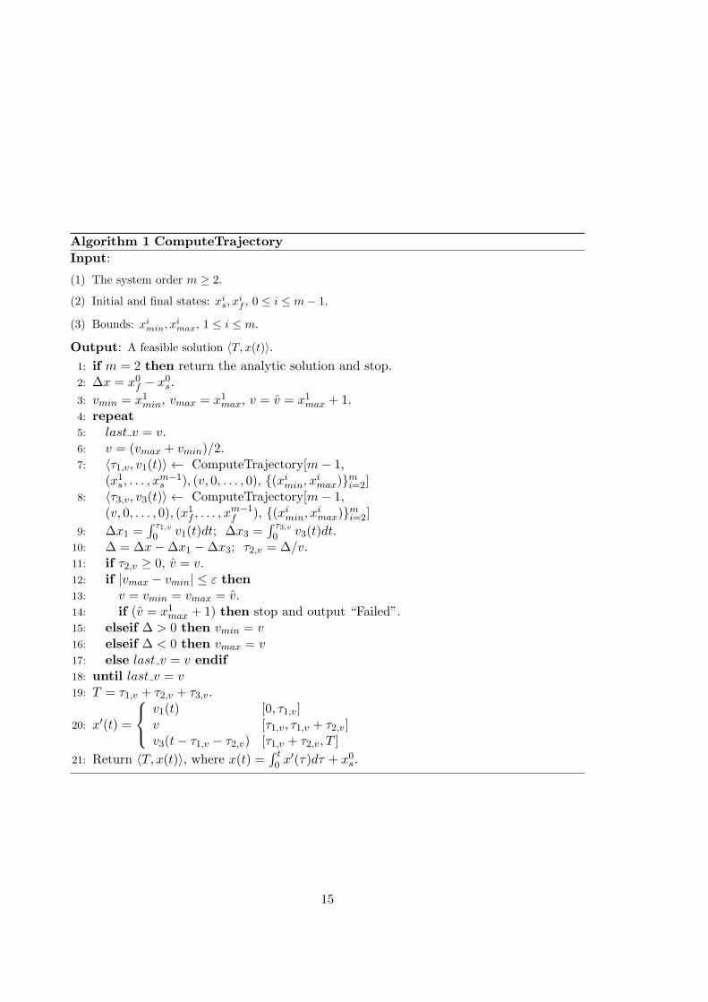
Algorithm 1 ComputeTrajectory
Input:
(1) The system order m ≥ 2.
(2) Initial and final states: xis, x
if , 0 ≤ i ≤ m− 1.
(3) Bounds: ximin, x
imax, 1 ≤ i ≤ m.
Output: A feasible solution ⟨T, x(t)⟩.1: if m = 2 then return the analytic solution and stop.2: ∆x = x0f − x0s.
3: vmin = x1min, vmax = x1max, v = v = x1max + 1.4: repeat5: last v = v.6: v = (vmax + vmin)/2.7: ⟨τ1,v, v1(t)⟩ ← ComputeTrajectory[m− 1,
(x1s, . . . , xm−1s ), (v, 0, . . . , 0), {(ximin, x
imax)}mi=2]
8: ⟨τ3,v, v3(t)⟩ ← ComputeTrajectory[m− 1,(v, 0, . . . , 0), (x1f , . . . , x
m−1f ), {(ximin, x
imax)}mi=2]
9: ∆x1 =∫ τ1,v0 v1(t)dt; ∆x3 =
∫ τ3,v0 v3(t)dt.
10: ∆ = ∆x−∆x1 −∆x3; τ2,v = ∆/v.11: if τ2,v ≥ 0, v = v.12: if |vmax − vmin| ≤ ε then13: v = vmin = vmax = v.14: if (v = x1max + 1) then stop and output “Failed”.15: elseif ∆ > 0 then vmin = v16: elseif ∆ < 0 then vmax = v17: else last v = v endif18: until last v = v19: T = τ1,v + τ2,v + τ3,v.
20: x′(t) =
v1(t) [0, τ1,v]v [τ1,v, τ1,v + τ2,v]v3(t− τ1,v − τ2,v) [τ1,v + τ2,v, T ]
21: Return ⟨T, x(t)⟩, where x(t) =∫ t0 x
′(τ)dτ + x0s.
15

Algorithm 2 SynchronizeTrajectories
Input:
(1) The system order m ≥ 1.
(2) The number n ≥ 1 of trajectories that need to be synchronized.
(3) An accuracy parameter for the motion time, θ ≥ 0.
(4) Initial values: xj,is , 0 ≤ i ≤ m− 1, 1 ≤ j ≤ n.
(5) Final values: xj,if , 0 ≤ i ≤ m− 1, 1 ≤ j ≤ n.
(6) Bounds: xj,imin ≤ 0 ≤ xj,i
max, 1 ≤ i ≤ m, 1 ≤ j ≤ n.
Output:
(1) Total motion time, T > 0.
(2) Trajectories xj(t), 1 ≤ j ≤ n, that satisfy the input constraints, each spanning the time T .
1: Tmax = 0; sync = 0.2: j = 1.3: repeat4: ⟨T, xj(t)⟩ ← ComputeTrajectory-TimeLimit[m,
(xj,0s , . . . , xj,m−1s ), (xj,0f , . . . , xj,m−1
f ), {(xj,imin, . . . , xj,imax)}mi=1, Text = Tmax]
5: if T − Tmax ≤ θ then sync = sync+ 16: else Tmax = T , sync = 17: j = j + 1.8: if j = n+ 1 then j = 19: until sync = n
10: Return ⟨Tmax, (x1(t), . . . , xn(t))⟩.
16

3.1 Examples of multi-axis trajectories
3.1.1 Example 1
This example demonstrates the use of Algorithm 2 to generate a trajectory that passesthrough four points in the plane with specified velocities and accelerations. The resultingtrajectory demonstrates the algorithm’s ability to produce a high order continuous path.
Let A = (0, 0), B = (20, 0), C = (20, 20), and D = (0, 20) be four points in the x − yplane. We wish to move a body through these points, A→ B → C → D → A, starting andfinishing at rest. We consider trajectories of order m = 3 with the following bounds alongeach of the four motion segments: |x(i)| ≤ 102+i, 1 ≤ i ≤ m.
We examine four scenarios that differ in the inner corner velocities and accelerations,at B, C and D. In Scenario 1, the body reaches a full stop in each inner corner beforecontinuing its motion. In Scenario 2, the velocity in each inner corner is 50 in the directionleading to the corner, and the acceleration there is zero. In Scenario 3, the corner velocitiesare counterclockwise 45o rotations of the corresponding corner velocities in Scenario 2 (sothat the velocity at B, for example, is (50/
√2, 50/
√2) instead of (50, 0) as it was in Scenario
2); the acceleration in each corner is set to zero. This adjustment of the velocity to theright-angle turn in each corner results in a shorter overall motion time with respect toScenario 2. Finally, Scenario 4 is identical to Scenario 2 except for the acceleration valuesin the inner corners. These acceleration values are designed so that the moving body beginsaccelerating for the next motion segment earlier, in order to reduce the overall motion time.The acceleration values are (−2000, 2000) at B, (−2000,−2000) at C, and (2000,−2000) atD. The trajectories in these scenarios are shown in Figure 7.
As expected, the motion time in Scenario 1 is the longest, T1 = 0.743. In Scenario 2,where the body is not forced to stop in each inner point, it is T2 = 0.701. In Scenario 3, inwhich the corner velocities are better adjusted to the counterclockwise turns in each corner,the motion time reduces to T2 = 0.683. Finally, in Scenario 4, with the added benefit ofacceleration conditions, the body completes the journey in time T4 = 0.620.
3.1.2 Example 2
This example demonstrates the use of Algorithm 2 to generate trajectories for a typical taskof a mobile robot that needs to pass through a few specified points at specified velocitiesand accelerations. Figure 8 show three trajectories that pass through the points: (0, 0),(2, 3), (4, 1), and (5, 5) at velocities (25, 7), (5, 3), (22, 25), and (14,−25). At each point,the velocity vector is marked by a line. The three trajectories differ in their order oftheir control input: third (m = 3), fourth (m = 4), and fifth (m = 5). The bounds onthe derivatives for both axes were set to: |x(1)| ≤ 1000, |x(2)| ≤ 10000, |x(3)| ≤ 100000,|x(4)| ≤ 5000000, |x(5)| ≤ 100000000. The rather large bounds for the higher derivativeswere chosen to allow the lower derivatives to reach higher values and get an overall fastermotion. It should be noted that large is a relative term here as for lower order trajectoriesthese values are effectively set to infinity.
All trajectories pass through the specified points at the specified velocities. They differ,however, in their smoothness and geometric path due to the larger number of switches ofthe higher order trajectories.
17

The fastest motion time of 0.3s was achieved by the third order trajectory; the motiontimes for the fourth and fifth order trajectories were 0.41s and 0.67s, respectively.
Figure 9 shows the acceleration along the y-axis for the third and fifth order trajectories.The high order trajectory is smoother, exerting, as a result, lower accelerations along thepath. This explains the differences in the geometric shape of the paths shown in Figure 8:the paths generated by lower order trajectories are visually smoother than those generatedby high order trajectories, because the higher accelerations applied by the lower ordertrajectory made it possible to connect the specified velocities with smooth curves, followedat high speeds; the higher order trajectories applied lower accelerations, which required toslow down before making the turn and accelerating to velocity at the next point. Thisillustrates the use of high order trajectories to limit the effort applied by the control systemwhile achieving the desired motion. In a real application, this limited effort will likely resultin a more accurate motion, smaller power consumption, and lower wear on the system.
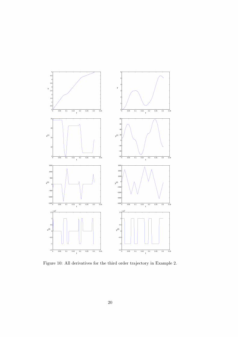
For completeness, Figure 10 shows all derivatives for the x and y axes in the exemplifiedthird order trajectory.
−1 0 1 2 3 4 5 6−1
0
1
2
3
4
5
6
x
y
m=5m=4m=3
Figure 8: Trajectories along a path.
18

0 0.05 0.1 0.15 0.2 0.25 0.3 0.35−4000
−3000
−2000
−1000
0
1000
2000
3000
t
y(2)
0 0.05 0.1 0.15 0.2 0.25 0.3 0.35 0.4 0.45−2500
−2000
−1500
−1000
−500
0
500
1000
1500
2000
t
y(2)
0 0.1 0.2 0.3 0.4 0.5 0.6 0.7−1000
−800
−600
−400
−200
0
200
400
600
800
1000
t
y(2)
Figure 9: Acceleration profiles for the third (top left) fourth (top right) and fifth (bottom)order trajectories in Example 2.
19
0 0.05 0.1 0.15 0.2 0.25 0.3 0.350
0.5
1
1.5
2
2.5
3
3.5
4
4.5
5
t
x
0 0.05 0.1 0.15 0.2 0.25 0.3 0.350
1
2
3
4
5
6
t
y
0 0.05 0.1 0.15 0.2 0.25 0.3 0.355
10
15
20
25
t
x(1)
0 0.05 0.1 0.15 0.2 0.25 0.3 0.35−60
−40
−20
0
20
40
60
80
t
y(1)
0 0.05 0.1 0.15 0.2 0.25 0.3 0.35−1500
−1000
−500
0
500
1000
1500
t
x(2)
0 0.05 0.1 0.15 0.2 0.25 0.3 0.35−4000
−3000
−2000
−1000
0
1000
2000
3000
t
y(2)
0 0.05 0.1 0.15 0.2 0.25 0.3 0.35−1.5
−1
−0.5
0
0.5
1
1.5x 10
5
t
x(3)
0 0.05 0.1 0.15 0.2 0.25 0.3 0.35−1.5
−1
−0.5
0
0.5
1
1.5x 10
5
t
y(3)
Figure 10: All derivatives for the third order trajectory in Example 2.
20

3.1.3 Example 3
In this example, a simple high level planner uses our algorithm to generate the trajectoriesfor a planar three-wheeled non-holonomic mobile robot. The underlying simulation engineused here is the ODE given in [27]. An executable file for running the simulation can befound at [6].
The trajectories are shown in Figure 11. Figure 12 shows a diagram of the robot. Theparameters of this robot are given in Table 3. It is controlled by specifying the longitudinalspeed v = ωr and the steering rate β(1), where ω is the rotational speed of the rear wheels,r is the wheel radius, and β is the steering angle of the front wheel. The bounds used forthe two control inputs are:
• |β(1)| < 5 [rad/s], |β(2)| < 10 [rad/s2], |β(3)| < 10 [rad/s3]
• |ω| < 5 [rad/s], |ω(1)| < 10 [rad/s2], |ω(2)| < 10 [rad/s3]
A high level planner then uses our algorithm to compute a sequence of control inputsthat would drive the robot to the target position from any given state. The trajectory inputparameters are determined by a simple state machine, which selects between three motionprimitives: (a) a straight line motion, (b) a right or left curve at a constant speed, and(c) a transition from a curve to a straight line. Alternating between these three motionprimitives, one can reach the target from any state. The handling of non-holonomic con-straints in this example is done indirectly by the interaction between the high level plannerand our algorithm. The high level planner reacts (online) to the current state and uses ouralgorithm to generate trajectory segments in an order that ensures reaching the goal. Thisexample demonstrates the use of our algorithm to generate a series of concatenated smoothtrajectories online as directed by a high level motion planner.
Component Dimensions [m] Weight [Kg]
Body 0.7× 0.5× 0.2 10Wheels 0.1 radius 0.2
Table 3: Robot parameters
The attached simulation shows the robot moving towards a randomly selected targetfrom a given initial state. The simulation demonstrates that by generating control inputs astrajectories of high order we can improve tracking accuracy as well as produce a smootherride. The simulation also shows that trajectories are not limited to simple XY-paths butcan be incorporated in many different applications.
21

−2.5−2−1.5−1−0.500.5−2
−1.5
−1
−0.5
0
0.5
1
1.5
y [m]
x [m] Start
Target
0 2 4 6 8 10 12 140
0.1
0.2
0.3
0.4
0.5
0.6
0.7
v[m/s]
t [s]
0 2 4 6 8 10 12 14−1.2
−1
−0.8
−0.6
−0.4
−0.2
0
0.2
β[rad]
t [s]0 2 4 6 8 10 12 14
−1.5
−1
−0.5
0
0.5
1
1.5
t [s]
β (1)
[rad/s]
Figure 11: The trajectories for β, v and the resulting XY path from (0, 0) to the target.
Figure 12: Top view of the simulated robot.
22
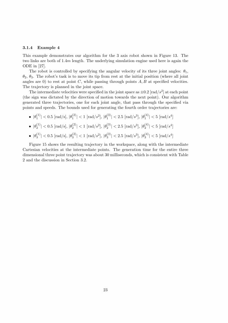
3.1.4 Example 4
This example demonstrates our algorithm for the 3 axis robot shown in Figure 13. Thetwo links are both of 1.4m length. The underlying simulation engine used here is again theODE in [27].
The robot is controlled by specifying the angular velocity of its three joint angles: θ1,θ2, θ3. The robot’s task is to move its tip from rest at the initial position (where all jointangles are 0) to rest at point C, while passing through points A,B at specified velocities.The trajectory is planned in the joint space.
The intermediate velocities were specified in the joint space as±0.2 [rad/s2] at each point(the sign was dictated by the direction of motion towards the next point). Our algorithmgenerated three trajectories, one for each joint angle, that pass through the specified viapoints and speeds. The bounds used for generating the fourth order trajectories are:
• |θ(1)1 | < 0.5 [rad/s], |θ(2)1 | < 1 [rad/s2], |θ(3)1 | < 2.5 [rad/s3], |θ(4)1 | < 5 [rad/s4]
• |θ(1)2 | < 0.5 [rad/s], |θ(2)2 | < 1 [rad/s2], |θ(3)2 | < 2.5 [rad/s3], |θ(4)2 | < 5 [rad/s4]
• |θ(1)3 | < 0.5 [rad/s], |θ(2)3 | < 1 [rad/s2], |θ(3)3 | < 2.5 [rad/s3], |θ(4)3 | < 5 [rad/s4]
Figure 15 shows the resulting trajectory in the workspace, along with the intermediateCartesian velocities at the intermediate points. The generation time for the entire threedimensional three point trajectory was about 30 milliseconds, which is consistent with Table2 and the discussion in Section 3.2.
23
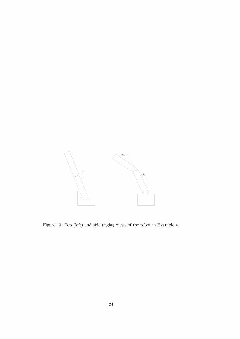
Figure 13: Top (left) and side (right) views of the robot in Example 4.
24

0 2 4 6 8 10 12 14 16 18−2.5
−2
−1.5
−1
−0.5
0
0.5
1
1.5
2
t
θ1
0 2 4 6 8 10 12 14 16 18
−0.5
−0.4
−0.3
−0.2
−0.1
0
0.1
0.2
0.3
0.4
0.5
t
θ1(1)
0 2 4 6 8 10 12 14 16 18−0.2
0
0.2
0.4
0.6
0.8
1
1.2
1.4
t
θ2
0 2 4 6 8 10 12 14 16 18−0.8
−0.6
−0.4
−0.2
0
0.2
0.4
0.6
t
θ2(1)
0 2 4 6 8 10 12 14 16 180
0.5
1
1.5
t
θ3
0 2 4 6 8 10 12 14 16 18−0.2
−0.1
0
0.1
0.2
0.3
0.4
0.5
0.6
t
θ3(1)
Figure 14: The joint angles and velocities for Example 4.
25

−2−1
01
2
−2
0
2
0
0.5
1
1.5
2
2.5
3
XY
Z
AB
C
Figure 15: The path followed by the robot’s tip and the Cartesian velocities at the viapoints in Example 4.
26
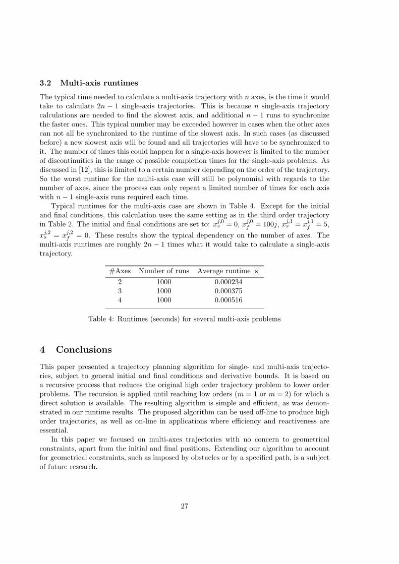
3.2 Multi-axis runtimes
The typical time needed to calculate a multi-axis trajectory with n axes, is the time it wouldtake to calculate 2n − 1 single-axis trajectories. This is because n single-axis trajectorycalculations are needed to find the slowest axis, and additional n − 1 runs to synchronizethe faster ones. This typical number may be exceeded however in cases when the other axescan not all be synchronized to the runtime of the slowest axis. In such cases (as discussedbefore) a new slowest axis will be found and all trajectories will have to be synchronized toit. The number of times this could happen for a single-axis however is limited to the numberof discontinuities in the range of possible completion times for the single-axis problems. Asdiscussed in [12], this is limited to a certain number depending on the order of the trajectory.So the worst runtime for the multi-axis case will still be polynomial with regards to thenumber of axes, since the process can only repeat a limited number of times for each axiswith n− 1 single-axis runs required each time.
Typical runtimes for the multi-axis case are shown in Table 4. Except for the initialand final conditions, this calculation uses the same setting as in the third order trajectoryin Table 2. The initial and final conditions are set to: xj,0s = 0, xj,0f = 100j, xj,1s = xj,1f = 5,
xj,2s = xj,2f = 0. These results show the typical dependency on the number of axes. Themulti-axis runtimes are roughly 2n − 1 times what it would take to calculate a single-axistrajectory.
#Axes Number of runs Average runtime [s]
2 1000 0.0002343 1000 0.0003754 1000 0.000516
Table 4: Runtimes (seconds) for several multi-axis problems
4 Conclusions
This paper presented a trajectory planning algorithm for single- and multi-axis trajecto-ries, subject to general initial and final conditions and derivative bounds. It is based ona recursive process that reduces the original high order trajectory problem to lower orderproblems. The recursion is applied until reaching low orders (m = 1 or m = 2) for which adirect solution is available. The resulting algorithm is simple and efficient, as was demon-strated in our runtime results. The proposed algorithm can be used off-line to produce highorder trajectories, as well as on-line in applications where efficiency and reactiveness areessential.
In this paper we focused on multi-axes trajectories with no concern to geometricalconstraints, apart from the initial and final positions. Extending our algorithm to accountfor geometrical constraints, such as imposed by obstacles or by a specified path, is a subjectof future research.
27
References
[1] J.E. Bobrow. Optimal robot path planning using the minimum time criterion. IEEETrans. Rob. Autom., 4(4):443–450, 1988.
[2] J.E. Bobrow, S. Dubowsky, and J.S. Gibson. Time-optimal control of robotic manip-ulators along specified paths. The International Journal of Robotics Research, 4(3):3,1985.
[3] X. Broquere, D. Sidobre, and I. Herrera-Aguilar. Soft motion trajectory plannerfor service manipulator robot. In Intelligent Robots and Systems, 2008. IROS 2008.IEEE/RSJ International Conference on, pages 2808–2813. IEEE, 2008.
[4] A.E. Bryson and Y.C. Ho. Applied Optimal Control. Blaisdell Publishing Co., Cam-bridge, MA, 1969.
[5] D. Costantinescu and E.A. Croft. Smooth and time-optimal trajectory planning forindustrial manipulators along specified paths. Journal of Robotic Systems, 17(5):233–249, 2000.
[6] B. Ezair, T. Tassa, and Z. Shiller. Robot application simulation. http://www.ariel.ac.il/sites/shiller/ravlab/online_trajectory/simulation.zip, 2013.
[7] C. Guarino Lo Bianco and O. Gerelli. Online trajectory scaling for manipulators subjectto high-order kinematic and dynamic constraints. Robotics, IEEE Transactions on,27(6):1144–1152, 2011.
[8] R. Haschke, E. Weitnauer, and H. Ritter. On-line planning of time-optimal, jerk-limited trajectories. In Intelligent Robots and Systems, 2008. IROS 2008. IEEE/RSJInternational Conference on, pages 3248–3253. IEEE.
[9] I. Herrera-Aguilar and D. Sidobre. On-line trajectory planning of robot manipulatorsend effector in cartesian space using quaternions. In 15th International Symposium onMeasurement and Control in Robotics, Belgium, November, 2005.
[10] I. Herrera-Aguilar and D. Sidobre. Soft motion trajectory planning and control for ser-vice manipulator robot. Workshop on Physical Human-Robot Interaction in AnthropicDomains at IROS, pages 13–22, 2006.
[11] T. Kroger, A. Tomiczek, and F.M. Wahl. Towards on-line trajectory computation. InIntelligent Robots and Systems, 2006 IEEE/RSJ International Conference on, pages736–741. IEEE, 2006.
[12] T. Kroger and F.M. Wahl. Online trajectory generation: basic concepts for instanta-neous reactions to unforeseen events. Robotics, IEEE Transactions on, 26(1):94–111,2010.
[13] P. Lambrechts, M. Boerlage, and M. Steinbuch. Trajectory planning and feedforwarddesign for high performance motion systems. In American Control Conference, 2004.Proceedings of the 2004, volume 5, pages 4637–4642. IEEE.
28

[14] S. Liu. An on-line reference-trajectory generator for smooth motion of impulse-controlled industrial manipulators. In Advanced Motion Control, 2002. 7th Interna-tional Workshop on, pages 365–370. IEEE, 2002.
[15] S. Macfarlane and E.A. Croft. Jerk-bounded manipulator trajectory planning: Designfor real-time applications. Robotics and Automation, IEEE Transactions on, 19(1):42–52, 2003.
[16] K.D. Nguyen, I.M. Chen, and T.C. Ng. Planning algorithms for s-curve trajectories.In Advanced intelligent mechatronics, 2007 IEEE/ASME international conference on,pages 1–6. IEEE, 2007.
[17] K. Petrinec and Z. Kovacic. Trajectory planning algorithm based on the continuity ofjerk. In Control & Automation, 2007. MED’07. Mediterranean Conference on, pages1–5. IEEE, 6.
[18] F. Pfeiffer and R. Johanni. A concept for manipulator trajectory planning. IEEETrans. on Robotics and Automation, RA-3(3):115–123, 1987.
[19] A. Piazzi and A. Visioli. Global minimum-jerk trajectory planning of robot manipula-tors. Industrial Electronics, IEEE Transactions on, 47(1):140–149, 2000.
[20] L.S. Pontryagin. The mathematical theory of optimal processes. In Intelligent Robotsand Systems, 2006 IEEE/RSJ International Conference on. Interscience, 1962.
[21] Z. Shiller. On singular time-optimal control along specified paths. IEEE Transactionson Robotics and Automation, 10(4), August 1994.
[22] Z. Shiller and H. Chang. Trajectory preshaping for high-speed articulated systems.In ASME Journal of Dynamic Systems, Measurement and Control, volume 117 No. 3,pages 304–310, September 1995.
[23] Z. Shiller and S. Dubowsky. Time-optimal path-planning for robotic manipulators withobstacles, actuator, gripper and payload constraints. Intl. J. Rob. Research, 8(6):3–18,Dec. 1989.
[24] Z. Shiller and H.H. Lu. Computation of path constrained time optimal motions withdynamic singularities. Journal of Dynamic Systems, Measurement and Control, 114:34–40, 1992.
[25] K.G. Shin and N.D. McKay. Minimum-time control of robotic manipulators withgeometric path constraints. IEEE Trans. Aut. Ctrl., AC-30(6):531–541, June 1985.
[26] J. Slotine and H. Yang. Improving the efficiency of time-optimal path-following algo-rithms. IEEE Transactions on Robotics and Automation, 5(1):118124, 1989.
[27] R. Smith. Open dynamics engine. http://www.ode.org, 2007.
[28] M. Tarkiainen and Z. Shiller. Time optimal motions of manipulators with actuatordynamics. In Proc. 1993 IEEE International Conference on Robotics and Automation,volume 2, pages 725–730, 1993.
29

A On the optimality of the solution
We prove herein the optimality of the solution produced by Algorithm 1 for m ≤ 3, in thecase where the initial and final conditions are zero, x1s = x1f = x2s = x2f = 0.
Lemma A.1. Consider the trajectory planning problem MP := MP(m;xs, xf , xmin, xmax)with zero initial and final conditions. Then the travel time of an optimal solution is strictlyincreasing with respect to the distance that needs to be traveled, |∆x| = |x0f − x0s|.
Proof. Without loss of generality, we assume that x0s = 0 and that x0f > 0. (The case
x0f < 0 can be reduced to the case x0f > 0.) Let ⟨T,X(t)⟩ be an optimal solution of
MP := MP(m;xs, xf , xmin, xmax), where xf = (x0f , 0, . . . , 0), and let ⟨T , X(t)⟩ be an opti-
mal solution of MP := MP(m;xs, xf , xmin, xmax) where xf = (x0f , 0, . . . , 0) and x0f > x0f .
Assume, towards contradiction, that T ≤ T . Set k = x0f/x0f < 1, and define the function
Z(t) = kX(k−1/mt). We claim, and prove below, that ⟨k1/mT , Z(t)⟩ is a solution of MP.However, since k1/mT < T ≤ T that would contradict the optimality of ⟨T,X(t)⟩.
To show that ⟨k1/mT , Z(t)⟩ is a solution of MP, we first observe that it satisfies therequired initial and final position requirements:
Z(0) = kX(0) = 0 ; Z(k1/mT ) = kX(k−1/mk1/mT ) = kX(T ) = kx0f = x0f .
Its derivatives are given by:
Z(i)(t) = k1−i/m · X(i)(k−1/mt) , 1 ≤ i ≤ m− 1 .
It is easy to see that all those derivatives vanish at t = 0 and t = k1/mT since all derivativesof X vanish at t = 0 and at t = T . It remains to show that the derivatives are properlybounded along the interval [0, k1/mT ]. Indeed, as k < 1:
maxt∈[0,k1/mT ]
k1−i/m · X(i)(k−1/mt) = k1−i/m · maxt∈[0,T ]
X(i)(t) ≤ k1−i/m · ximax < ximax ,
whence Z respects the upper bounds xmax. Similarly, it respects also the lower boundsxmin. The proof is thus complete.
Lemma A.2. Consider the trajectory planning problem MP := MP(m ≤ 2;xs, xf , xmin, xmax),where x1s = x1f = 0, and let ⟨T,X(t)⟩ be an optimal solution. Let Y (t) be a function thatsatisfies the initial conditions xs, and its derivatives are bounded by xmax and xmin. Thenif Y (T ) ≤ X(T ), it holds that Y (t) ≤ X(t) for all t ∈ [0, T ].
Proof. Assume, towards contradiction, that Y (t) > X(t) for some t ∈ [0, T ]. Then, asY (0) = X(0) and Y (T ) ≤ X(T ), the difference Y (t)−X(t) must have a positive maximumin (0, T ), say at t = t0. Define
Z(t) =
{Y (t) t ∈ [0, t0] ,X(t) + Y (t0)−X(t0) t ∈ [t0, T ] .
We claim, and prove below, that ⟨T,Z(t)⟩ is a solution to MP := MP(m;xs, xf , xmin, xmax)where xf = (x0f , 0) and x0f > x0f . However, that is impossible in view of Lemma A.1.
30

Clearly, Z satisfies the initial conditions xs, since Y does. As for the final conditions,Z(T ) = x0f := X(T ) + Y (t0) − X(t0) > X(T ) = x0f , and Z ′(T ) = X ′(T ) = 0 (recall thatm = 2 so the initial and final conditions are only on the position and velocity). It remainsto show that the derivatives of Z are properly bounded. Its derivatives are bounded byxmin and xmax on [0, t0] since Y is, and they are bounded on [t0, T ] since X is. Whenm = 1, that completes the proof (since in that case it is only needed to show that the firstderivative is bounded, but there is no need to show that it is continuous). When m = 2,we need to show that Z ′ is continuous at t0. That is indeed the case since, as the functionY (t)−X(t) reaches a maximum value at t0, it holds that Y
′(t0) = X ′(t0).
Lemma A.3. Consider the two problems MPi = MP(m ≤ 2;xs, xf , xmin, xmax), i = 1, 2,where xfi = (ei, 0). Let ⟨Ti, Xi(t)⟩ be an optimal solution to MPi, i = 1, 2. Then if e1 ≥ e2,
it holds that∫ T1
0 X1(t)dt ≥∫ T2
0 X2(t)dt.
Proof. Assume that e1 ≥ e2. Then, by Lemma A.1, T1 ≥ T2. Let us extend the functionX2 to the interval [0, T1] as follows:
X2(t) =
{X2(t) t ∈ [0, T2] ,e2 t ∈ [T2, T1] .
It is easy to see that ⟨T1, X2(t)⟩ is another solution to MP2. (When m = 1 this is simple;when m = 2, we have X ′
2(T2) = 0, whence X2(t) has a continuous derivative along [0, T1].)By Lemma A.2 on X1(t) and X2(t), we get that X2(t) ≤ X1(t) for all 0 ≤ t ≤ T1. Hence,∫ T1
0X1(t)dt ≥
∫ T1
0X2(t)dt ≥
∫ T2
0X2(t)dt .
Finally, we prove that when m ≤ 3 and the initial and final conditions are zero, Algo-rithm 1 produces a solution which approximates an optimal solution.
Theorem A.4. Consider the trajectory planning problem MP(m ≤ 3;xs, xf , xmin, xmax)with zero initial and final conditions, x1s = x1f = x2s = x2f = 0. Let ⟨T,X(t)⟩ be an optimalsolution for which v0 := max[0,T ]X
′ is maximal (from among all optimal solutions for theproblem). Then the solution x(t) = xε(t) generated by Algorithm 1 converges to X(t) whenε→ 0.
Proof. The theorem is true for m = 1 since the solution that it returns in that case isclearly optimal. We proceed by induction. Without loss of generality, we assume that∆x = x0f − x0s > 0. (The case ∆x < 0 can be reduced to the case ∆x > 0.) In such cases,the algorithm will reject all values of v ≤ 0 since for such values the resulting velocity willbe always non-positive, whence cannot travel a positive distance ∆x.
Let v0 be the maximum of X ′(t) on [0, T ]. Consider now the sequence of values of vthat are tested in the binary search by Algorithm 1. For some of those values the algorithmmanages to construct a valid solution (when ∆/v ≥ 0), while for others it fails (when ∆/v <0). If v is a value for which the algorithm managed to find a valid solution, we shall denotethat solution by ⟨Tv, xv(t)⟩. We will show that v → v0 and that ⟨Tv, xv(t)⟩ → ⟨T,X(t)⟩. Tothis end, we prove the following claims:
31
C1: If v is a value that the algorithm accepts, then ⟨Tv, xv(t)⟩ is the optimal solution fromamong all solutions for which the first derivative is upper bounded by v.
C2: In the binary search, every v > v0 will be rejected by the algorithm.
C3: In the binary search, every 0 < v ≤ v0 will be accepted by the algorithm.
C4: When v → v0, ⟨Tv, xv(t)⟩ → ⟨T,X(t)⟩.
• Proving C1: The solution ⟨Tv, xv(t)⟩ constructed by the algorithm for the value v hasa derivative x′v(t) with the following structure:
x′v(t) =
v1(t) [0, τ1,v] ,v [τ1,v, τ2,v + τ1,v] ,v3(t− τ2,v − τ1,v) [τ2,v + τ1,v, Tv] .
Since, by induction, the algorithm returns the optimal solution for m− 1, then ⟨τ1,v, v1(t)⟩is an optimal solution for the reduced MP problem described in Step 7 of the algorithm.
Assume that ⟨Tg, g(t)⟩ is another solution MP for which Tg ≤ Tv and max g′ ≤ v. Weshall prove that in such a case g coincides with xv. By Lemma A.2, for x′v and g′ (as X andY respectively), g′(t) ≤ x′v(t) for all t ∈ [0, τ1,v]. Hence,∫
[0,τ1,v ]g′(t)dt ≤
∫[0,τ1,v ]
x′v(t)dt . (12)
Applying Lemma A.2 for x′v(Tv − t) and g′(Tg − t) on [0, τ3,v] we infer that g′(Tg − t) ≤x′v(Tv − t) for all t ∈ [0, τ3,v], whence∫
[0,τ3,v ]g′(Tg − t)dt ≤
∫[0,τ3,v]
x′v(Tv − t)dt . (13)
Consider now the interval
I = [0, Tg] \([0, τ1,v]
∪[Tg − τ3,v, Tg]
). (14)
Since Tg ≤ Tv, that interval is contained in the interval [τ1,v, Tv−τ3,v] along which x′v(t) = v.Hence, as g′ ≤ v, ∫
Ig′(t)dt ≤
∫Ix′v(t)dt . (15)
Adding up inequalities (12)–(15), we infer that∫ Tg
0g′(t) ≤
∫[0,τ1,v ]
x′v(t)dt+
∫[0,τ3,v ]
x′v(Tv − t)dt+
∫Ix′v(t)dt . (16)
The integral on the left of (16) is the total distance covered by g along the time interval[0, Tg]; therefore it equals ∆x. The sum of integrals on the right of (16) equals∫ Tv
0x′v(t)dt+ δ = ∆x+ δ where δ :=
(∫Ix′v(t)dt−
∫ Tv−τ3,v
τ1,v
x′v(t)dt
).
32

The definition of the interval I, (14), and the assumption Tg ≤ Tv, imply that I is containedin [τ1,v, Tv− τ3,v]. Since x
′v = v > 0 along the latter interval, it follows that δ ≤ 0 and δ = 0
if and only if Tg = Tv. To summarize, the left hand side in inequality (16) equals ∆x andthe right hand side equals ∆x + δ, for δ ≤ 0. The only way for the inequality to hold isif δ = 0, i.e. Tg = Tv. Therefore, g′ and x′v are two continuous functions on [0, Tv] whereg′(t) ≤ x′v(t) for all t ∈ [0, Tv] and their integrals along the interval coincide. This can occurif and only if g′ = x′v for all t. Since g(0) = xv(0) = 0, we infer that g and xv coincide.
• Proving C2: Assume, towards contradiction, that the algorithm produced a validsolution X(t) with maximal velocity v > v0. By C1, X(t) is at least as good as all othersolutions whose maximal velocity is bounded from above by v. But X(t) is such a solution.Hence, since X(t) is an optimal solution, so is X(t). But that contradicts our assumptionthat X(t) is an optimal solution that maximizes maxX ′.
• Proving C3: In testing a value v, the algorithm finds, by recursion, the optimal solutionto the problem
MP(m− 1; (0, 0), (v, 0), (x1min, . . . , xmmin), (x
1max, . . . , x
mmax)) .
Let us denote that solution by ⟨τ1,v, v1,v⟩. Similarly, ⟨τ3,v, v3,v⟩ is the optimal solution tothe problem
MP(m− 1; (v, 0), (0, 0), (x1min, . . . , xmmin), (x
1max, . . . , x
mmax)) .
Let y(t) denote the concatenation of v1,v0 and v3,v0 , i.e.,
y(t) =
{v1,v0(t) t ∈ [0, τ1,v0 ] ,v3,v0(t− τ1,v0) t ∈ [τ1,v0 , τ1,v0 + τ3,v0 ] .
Since τ1,v0 is smaller than the time it takes X ′ to reach v0 (owing to the optimality of⟨τ1,v0 , v1,v0⟩), and, similarly for the decreasing part of the profile, the time interval on whichy is defined is smaller than T (the interval on which X is defined). Hence, by Lemma A.1,the distance covered by Y (t) =
∫ t0 y(τ)dτ does not exceed ∆x, the distance covered by X.
By Lemma A.3, as v ≤ v0,∫ τ1,v
0v1,v(t)dt ≤
∫ τ1,v0
0v1,v0(t)dt .
In similarity, the integral of v3,v in the third interval will be at most the integral of v3,v0 .Therefore, the distance covered by v1,v and v3,v does not exceed ∆x. But then ∆ = ∆(v) ≥0, whence the algorithm would accept v.
• Proving C4: By C2 and C3, the sequence v that the algorithm accepts must converge tov0. By C3, the algorithm would accept the value v0; the corresponding constructed solution,⟨Tv0 , xv0⟩, is the optimal solution X(t), as implied by C1. Hence, we only need to showthe continuous dependence of ⟨Tv, xv⟩ on v. But this is trivial, since the explicit solutionfor x′v on the first and third intervals depend continuously on v) and hence, when v → v0,Tv → Tv0 and x′v(t) → x′v0(t) for all t. By integration, we conclude that xv(t) → xv0(t) forall t.
33
Corollary A.5. Under the conditions of Theorem A.4, the optimal solution ⟨T,X(t)⟩ isunique.
Proof. Assume that there exists more than one optimal solution and let v0 be as definedin Theorem A.4. By C3 in the proof of the theorem, Algorithm 1 would accept the valuev0 and return a solution ⟨Tv0 , xv0⟩. By C1 in the proof, any other solution to the problemwhose first derivative is bounded by v0 must coincide with ⟨Tv0 , xv0⟩. Hence, ⟨Tv0 , xv0⟩ isthe unique optimal solution.
A.1 Non-optimality in the general case
We showed in which cases the algorithm’s solution is guaranteed to be optimal. Here, weexamine the cases when the solution found by the algorithm may not be optimal. There aretwo assumptions made to make the search for the solution faster and more efficient. Theseassumptions, however, are not always true, and there are (somewhat rare) instances whenthey may mislead the algorithm into missing the optimal solution.
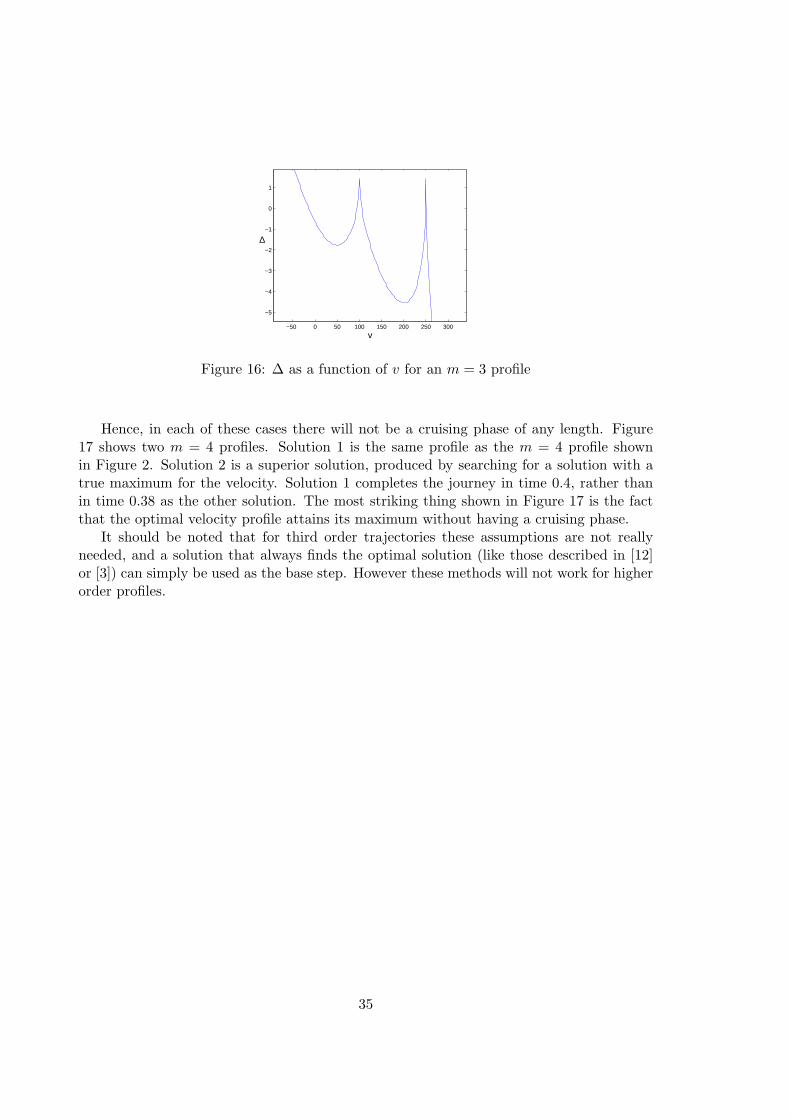
The first assumption may cause the optimal solution to be missed when dealing withthird order (or higher) profiles with non-zero initial or final conditions. When we searchfor the optimal cruising velocity (the value v in the algorithm), we are looking for thevelocity that will yield the lowest ∆, which is the distance covered during the constantvelocity phase. By minimizing ∆, we cover more of the total distance while accelerating(or decelerating), which results in a faster profile. However, an underlying assumption thatthe algorithm makes implicitly is that ∆ is monotonically non-increasing with respect to v,the cruising velocity. This is indeed true for zero initial and final conditions, but it is notalways so otherwise. Figure 16 shows ∆ as a function of the cruising velocity for a thirdorder profile, which uses the same parameters as the third order profile in figure 2, exceptfor W = 15, x1s = 250, and x1f = 100. These nonzero initial and final conditions give riseto two singularities in ∆(v), as the figure clearly shows. More importantly, the profile isnot monotonic, as assumed by the algorithm. In particular, while a monotonic functionattains the value 0 at most once, a non-monotonic function may attain it several times —five times in the function shown. Hence, while the algorithm uses a simple binary searchto find the supposedly single zero of ∆(v), here, the existence of several zeros may leadthe algorithm into an arbitrary one of those zeros, and not necessarily the one which yieldsminimal motion time.
The second assumption may affect third order profiles with non-zero initial or finalconditions, or problem instances with m ≥ 4. This time, the problem is in assuming thatthere is a cruising phase at all (even a degenerate one with 0 time). This assumption isshared by other works that produce higher than third order profiles, e.g. [16]. By assuminga cruising phase, we know that there is a point in the profile where all derivatives otherthan the velocity are 0. This greatly simplifies the search as we only have to search for anoptimal cruising velocity rather than a state vector of length m. However, if the optimaltrajectory always accelerates (or decelerates) then there will be no cruising phase. Also, ifm ≥ 4, the velocity profile may attain a true maximum (or minimum) velocity, and whilein such points the acceleration is indeed zero (as it is the first derivative of the velocity), atleast one higher derivatives will not be.
34
−50 0 50 100 150 200 250 300
−5
−4
−3
−2
−1
0
1
v
∆
Figure 16: ∆ as a function of v for an m = 3 profile
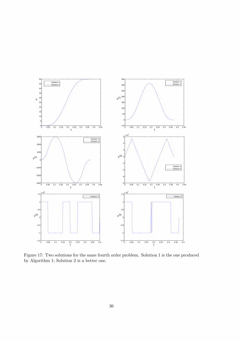
Hence, in each of these cases there will not be a cruising phase of any length. Figure17 shows two m = 4 profiles. Solution 1 is the same profile as the m = 4 profile shownin Figure 2. Solution 2 is a superior solution, produced by searching for a solution with atrue maximum for the velocity. Solution 1 completes the journey in time 0.4, rather thanin time 0.38 as the other solution. The most striking thing shown in Figure 17 is the factthat the optimal velocity profile attains its maximum without having a cruising phase.
It should be noted that for third order trajectories these assumptions are not reallyneeded, and a solution that always finds the optimal solution (like those described in [12]or [3]) can simply be used as the base step. However these methods will not work for higherorder profiles.
35
0 0.05 0.1 0.15 0.2 0.25 0.3 0.35 0.4 0.450
5
10
15
20
25
30
35
40
45
50
t
x
Solution 1Solution 2
0 0.05 0.1 0.15 0.2 0.25 0.3 0.35 0.4 0.45−50
0
50
100
150
200
250
300
350
t
x(1)
Solution 1Solution 2
0 0.05 0.1 0.15 0.2 0.25 0.3 0.35 0.4 0.45−3000
−2000
−1000
0
1000
2000
3000
t
x(2)
Solution 1Solution 2
0 0.05 0.1 0.15 0.2 0.25 0.3 0.35 0.4 0.45−8
−6
−4
−2
0
2
4
6x 10
4
t
x(3)
Solution 1Solution 2
0 0.05 0.1 0.15 0.2 0.25 0.3 0.35 0.4−1.5
−1
−0.5
0
0.5
1
1.5x 10
6
t
x(4)
Solution 1
0 0.05 0.1 0.15 0.2 0.25 0.3 0.35 0.4−1.5
−1
−0.5
0
0.5
1
1.5x 10
6
t
x(4)
Solution 2
Figure 17: Two solutions for the same fourth order problem. Solution 1 is the one producedby Algorithm 1; Solution 2 is a better one.
36