planetary radio interferometry and doppler …. duev et al.: planetary radio interferometry and...

Astronomy & Astrophysics manuscript no. 28869 c©ESO 2016June 21, 2016

Planetary Radio Interferometry and Doppler Experiment (PRIDE)technique: A test case of the Mars Express Phobos fly-by.

D.A. Duev1, 2, 3, S.V. Pogrebenko2, G. Cimò2, 4, G. Molera Calvés5, 2, T.M. Bocanegra Bahamón6, 2, 7, L.I. Gurvits2, 6,M.M. Kettenis2, J. Kania8, 2, V. Tudose9, P. Rosenblatt10, J.-C. Marty11, V. Lainey12, P. de Vicente13, J. Quick14,

M. Nickola14, A. Neidhardt15, G. Kronschnabl15, C. Ploetz15, R. Haas16, M. Lindqvist16, A. Orlati17, A.V. Ipatov18,M.A. Kharinov18, A.G. Mikhailov18, J.E.J. Lovell19, J.N. McCallum19, J. Stevens20, S.A. Gulyaev21, T. Natush21,

S. Weston21, W.H. Wang7, B. Xia7, W.J. Yang22, L.-F. Hao23 J. Kallunki24, and O. Witasse25

1 California Institute of Technology, 1200 E California Blvd, Pasadena, CA 91125, USAe-mail: [email protected]

2 Joint Institute for VLBI ERIC, P.O. Box 2, 7990 AA Dwingeloo, The Netherlands3 Sternberg Astronomical Institute, Lomonosov Moscow State University, Universitetsky av. 13, 119991 Moscow, Russia4 ASTRON, the Netherlands Institute for Radio Astronomy, Postbus 2, 7990 AA, Dwingeloo, The Netherlands5 Aalto University, School of Electrical Engineering, Department of Radio Science and Engineering, 02150 Espoo, Finland6 Department of Astrodynamics and Space Missions, Delft University of Technology, 2629 HS Delft, The Netherlands7 Shanghai Astronomical Observatory, 80 Nandan Road, Shanghai 200030, China8 Carnegie Mellon University, 5000 Forbes Ave, Pittsburgh, PA 15213, USA9 Institute for Space Sciences, Atomistilor 409, P.O. Box MG-23, Bucharest-Magurele RO-077125, Romania

10 Royal Observatory of Belgium, Ringlaan 3, 1180 Brussels, Belgium11 CNES/GRGS, OMP 14 avenue Edouard Belin 31400 Toulouse, France12 IMCCE, Observatoire de Paris, PSL Research University, CNRS-UMR8028 du CNRS, UPMC, Lille-1, 77 Av. Denfert-Rochereau,

75014, Paris, France13 Observatorio de Yebes (IGN), Apartado 148, 19180, Guadalajara, Spain14 Hartebeesthoek Radio Astronomy Observatory, 1740 Krugersdorp, South Africa15 Federal Agency for Cartography and Geodesy, Geodetic Observatory of Wettzell, 60598 Frankfurt Am Main, Germany16 Department of Earth and Space Sciences, Chalmers University of Technology, Onsala Space Observatory, 439 92 Onsala, Sweden17 National Institute for Astrophysics, Radio Astronomy Institute, Radio Observatory Medicina, 75500 Medicina, Italy18 Institute of Applied Astronomy, Russian Academy of Sciences, Kutuzova Embankment 10, 191187 Saint-Petersburg, Russia19 School of Physical Sciences, University of Tasmania, Private Bag 37, Hobart, 7001, Australia20 CSIRO Astronomy and Space Science, Australia Telescope National Facility, Narrabri NSW 2390, Australia21 Institute for Radio Astronomy and Space Research, Auckland University of Technology, Private Bag 92006, Auckland 1142, New

Zealand22 Xinjiang Astronomical Observatory, Chinese Academy of Sciences, 830011 Urumqi, PR China23 Yunnan Astronomical Observatory, Chinese Academy of Sciences, 650011 Kunming, PR China24 Metsähovi Radio Observatory, Aalto University, 02540 Kylmälä, Finland25 European Space Agency, ESA/ESTEC Scientific Support Office, 2200AG Noordwijk, The Netherlands

Received 7 May 2016 / accepted 31 May 2016

ABSTRACT

Context. The closest ever fly-by of the Martian moon Phobos, performed by the European Space Agency’s Mars Express spacecraft,gives a unique opportunity to sharpen and test the Planetary Radio Interferometry and Doppler Experiments (PRIDE) technique inthe interest of studying planet - satellite systems.Aims. The aim of this work is to demonstrate a technique of providing high precision positional and Doppler measurements ofplanetary spacecraft using the Mars Express spacecraft. The technique will be used in the framework of Planetary Radio Interferometryand Doppler Experiments in various planetary missions, in particular in fly-by mode.Methods. We advanced a novel approach to spacecraft data processing using the techniques of Doppler and phase-referenced verylong baseline interferometry spacecraft tracking.Results. We achieved, on average, mHz precision (30 µm/s at a 10 seconds integration time) for radial three-way Doppler estimatesand sub-nanoradian precision for lateral position measurements, which in a linear measure (at a distance of 1.4 AU) corresponds to∼ 50 m.

Key words. astrometry – techniques: interferometric – instrumentation: interferometers – instrumentation: miscellaneous

1. Introduction

The Planetary Radio Interferometry and Doppler Experiments(PRIDE) project (Duev et al. 2012) initiated by the Joint Institute

for VLBI ERIC (JIVE, Dwingeloo, The Netherlands) utilisesDoppler and phase-referencing very long baseline interferomet-

Article number, page 1 of 9

arX

iv:1

606.

0584

1v1

[as

tro-

ph.I

M]

19

Jun

2016

A&A proofs: manuscript no. 28869

ric (VLBI1) observations to provide high precision spacecraftstate vector estimation. In this paper, we further advance a novelapproach to spacecraft data processing developed within PRIDE.

On December 29, 2013, the European Space Agency’s MarsExpress (MEX) spacecraft made the closest ever fly-by of Pho-bos, one of the two Martian moons, just some 45 km from itssurface (Witasse et al. 2014). PRIDE observations of MEX dur-ing this event, involving more than 30 radio telescopes spreadaround the globe, were carried out by our team on December 28-29, 2013 (PI Pascal Rosenblatt, Royal Observatory of Belgium;European VLBI Network (EVN)/Global VLBI experiment codeGR035). These observations allow reconstructing MEX’s trajec-tory in the vicinity of Phobos with a high accuracy, which willin turn help to put a better constraint on the geophysical parame-ters of Phobos, possibly shedding light on its origin. The PRIDEdata processing technique has been specifically refined for theobservations of MEX during this event to provide high preci-sion positional and Doppler measurements. In particular, we de-scribe here the improvements made to the correlator softwareat JIVE (Keimpema et al. 2015) that allow efficient handling ofsuch data, and we demonstrate the positive impact of these en-hancements on the spacecraft position estimates obtained at thepost-processing stage. The use of the Doppler and VLBI data indynamical modelling of MEX motion to estimate the geophys-ical parameters related to the interior composition of this Marsmoon is discussed in Rosenblatt et al. (2016, in prep.).

The GR035 experiment has been conducted as a live end-to-end verification of the PRIDE technique which will be used infuture planetary missions, in particular ESA’s Jupiter Icy Satel-lites Explorer, JUICE (Grasset et al. 2013). In this paper, wepresent the technique, including the data processing algorithms.In Section 2, we describe the set-up of the GR035 experiment.Section 3 describes Doppler and VLBI data processing pipelineand presents the results of the experiment. Section 4 provides thereader with conclusions and outlook. The scientific evaluation ofthe experiment will be given in a separate paper (Rosenblatt etal., in prep.). The experiment GR035 was complementary to thenominal MEX Radio Science experiment MaRS (Pätzold et al.2004; Pätzold et al. 2016).

2. Experiment GR035 set-up

The error in the a priori position of a phase calibrator directlyaffects the estimates of the MEX orbit parameters proportion-ally to the separation angle between the calibrator and the tar-get. Therefore, in order to reach the best positional accuracy ofMEX achievable with the modern ground-based VLBI – abouta nanoradian (0.2 mas), which is translated to ∼100 metres atthe orbit, phase calibrators are necessary within ∼2o (Beasley &Conway 1995) of the MEX position at the observational epochwith absolute errors in their position not exceeding 0.2 mas.

In the case of the GR035 experiment, the timing of the ob-servations and therefore the sky position of the events were, ob-viously, defined by MEX ballistics. The nearest bright sourcesuitable as a primary phase calibrator, J1232−0224, with 0.16mas error in RA, 0.27 mas error in Dec, and 0.717 Jy total X-band flux density (Petrov 2015), happened to be at a fairly largeangular distance of ∼2.5o from the target. For this reason, onMarch 19, 2013, we performed VLBI observations of the fly-by

1 Very long baseline interferometry (VLBI) is a technique in which thesignals from a network of radio telescopes, spread around the world, arecombined to simulate one single telescope with a resolution far surpass-ing that of the individual telescopes.

Fig. 1. Mars Express Phobos fly-by experiment field on the sky. A largeblack star denotes the field centre; three crosses denote the pointingsused in the experiment ET027 to observe possible secondary calibra-tors; five smaller black stars denote the detected sources; the circle rep-resents the approximate size of the primary beam of a 30 m antenna.The colour insets show calibrated images of three of the sources in thefield obtained in the ET027 experiment.

event field with the EVN (experiment code ET027). We wereable to identify three new sources, one of which – ‘CAL5’ orJ1243−0218 (0.133 Jy total flux density; see Fig. 1) – appearedto be suitable both as a secondary calibrator and as an arc sta-bility test source to ensure the quality of the final astrometricalsolution for MEX.

The observations of the fly-by event were carried out withinthe global VLBI experiment GR035. During the run on Decem-ber 28-29, 2013, we observed three consecutive revolutions ofMEX around Mars, each 7 hours long, in order to provide a bet-ter coverage for further orbit reconstruction. The total durationof the experiment was 25 hours. Telescopes that took part in theobservations2 were split into two sub-arrays. The antennas inthe first sub-array (see Fig. 2, stations depicted with triangles)observed in Doppler mode with a dual S/X-band (2/8.4 GHz)frequency set-up with long scans (20-minutes) to minimise theDoppler frequency detection noise. The second sub-array an-tennas (see Fig. 2, stations depicted with circles) used an X-band (8.4 GHz) set-up and operated in a phase-referencing VLBImode with short scans (Ros et al. 1999), alternating between thetarget and the phase calibrators. The frequency set-up used byeach of the stations is shown in Fig. 2. Standard VLBI record-ing equipment was used at all stations. Strong sources M87 andJ1222+0413 with total X-band flux densities of 1.968 and 0.701Jy, respectively (Petrov 2015), were used as fringe3 finders.

The Australian, New Zealand and eastern EVN stations be-gan the tracking, then subsequently the western EVN and VLBAstations stepped in. This is illustrated in Fig. 3.


D.A. Duev et al.: Planetary Radio Interferometry and Doppler Experiment (PRIDE) technique: A test case of the Mars Express Phobos fly-by.

Fig. 2. Experiment GR035: participating telescopes are denoted by their two-letter codes. Stations depicted with a triangle were engaged in theDoppler part of the experiment, with a circle in the phase-referencing VLBI part. Station colour denotes frequency set-up used: red – 8332 – 8444MHz, 8 channels of 16 MHz USB (Upper Side Band); blue – 8396 – 8444 MHz, 4 channels of 16 MHz USB; orange – 8380 – 8428 MHz, 4channels of 16 MHz USB; green – 2289 – 2305 / 8396 – 8412 MHz, 4 channels of 16 MHz USB.

Fig. 3. Observational time ranges (UTC) of the telescopes that partic-ipated in the phase-referencing VLBI part. Green indicates the Aus-tralian, New Zealand and eastern EVN stations, blue the western EVNstations, and red the VLBA stations. Station codes as in Fig. 2. Thedashed black vertical line denotes the time of the fly-by event as seenfrom the Earth.

3. Doppler and VLBI data processing pipeline andresults

We have advanced the generic spacecraft data processingpipeline developed within the scope of PRIDE (outlined in Fig.4) to achieve a very high precision of MEX positional estima-tion, which is shown schematically in Fig. 5.

First, we performed narrowband processing of the single-dish open-loop data collected by all of the stations. We used the

2 Additional information about particular antennas can be found bythe two-letter codes shown in Fig. 2 in the databases of, e.g. theInternational VLBI Service at ftp://ivscc.gsfc.nasa.gov/pub/control/ns-codes.txt and the European VLBI Network at http://www.evlbi.org/user_guide/EVNstatus.txt3 The response of a VLBI system.

Fig. 4. Generic PRIDE data flow and processing pipeline. SpacecraftDoppler and delay observables obtained, respectively, at the narrow-band and post-processing steps, alongside the final astrometric solu-tion, that can be used for a variety of scientific applications (Duev et al.2012).

SWSpec/SCtracker/dPLL4 (Molera Calvés 2012; Molera Calvéset al. 2014) software package to obtain the topocentric Dopplerdetections. SWSpec extracts the raw data from the channelwhere the spacecraft carrier signal is expected to be recorded.Then it performs a window-overlapped add (WOLA) discreteFourier transform (DTF) and time integration over the obtainedspectra. The result is an initial estimate of the spacecraft carriertone along the scan. The moving phase of the spacecraft carriertone throughout the scan is modelled by performing an n-order

4 Wagner, J., Molera Calvés, G., and Pogrebenko, S.V. 2009-2014,Metsähovi Software Spectrometer and Spacecraft Tracking tools, Soft-ware Release, GNU GPL, http://www.metsahovi.fi/en/vlbi/spec/index


ftp://ivscc.gsfc.nasa.gov/pub/control/ns-codes.txt

ftp://ivscc.gsfc.nasa.gov/pub/control/ns-codes.txt

http://www.evlbi.org/user_guide/EVNstatus.txt

http://www.evlbi.org/user_guide/EVNstatus.txt

http://www.metsahovi.fi/en/vlbi/spec/index

http://www.metsahovi.fi/en/vlbi/spec/index


Fig. 5. GR035 data processing pipeline. The positional measurementsand the Doppler detections are fed into a dynamical model of MEXmotion (Rosenblatt et al. 2016, in prep.).

Fig. 6. Doppler detection noise in mHz at X-band. Topocentric detec-tions with a 10-second integration time for each station were differencedwith predicted values, and the standard deviation of the result was cal-culated for each 2-minute scan providing what is referred to as the mea-surements in the histogram.

frequency polynomial fit. SCtracker uses this initial fit to stopthe phase of the carrier tone, allowing subsequent tracking, fil-tering and extraction of the carrier tone in narrower bands (fromthe initial 16 MHz channel bandwidth down to a 2 kHz band-width) using a second-order WOLA DFT-based algorithm ofthe Hilbert transform approximation. The Digital Phase-Locked-Loop (dPLL) performs high precision reiterations of the previoussteps – time-integration of the overlapped spectra, phase polyno-mial fitting, and phase-stopping correction – on the 2 kHz band-width signal, using 20000 FFT points and 10-second integrationtime. The output of the dPLL is the filtered down-converted sig-nal and the final residual phase in the stopped band with respectto the initial phase polynomial fit. The bandwith of the out-put detections is 20 Hz with a frequency spectral resolution of2 mHz. The Doppler observable is obtained by adding the basefrequency of the selected channel to the 10-second averaged car-rier tone frequencies retrieved by the dPLL.

During this experiment, three transmitting stations provided24-hour coverage: the 35-metre ESTRACK station New Nor-cia (NNO) in Australia and the 70-metre Deep Space Stations63 (DSS-63) in Robledo (Spain) and 14 (DSS-14) in Gold-stone (CA, USA). In order to estimate the Doppler noise fn, thetopocentric detections with a 10-second integration time for eachstation were differenced with predicted three-way Doppler val-ues, and the standard deviation of the result was calculated for

Fig. 8. Zoom into the carrier line without (left panel) and with theDoppler phase correction (right panel). 10 sec integration time, 215 =32768 points spectral resolution, baseline Hh-Ww, scan 135. 23:22 –23:24 UTC, December 28, 2013.

each 2-minute scan (see the histogram in Fig 6). The resultingmean value of fn is 2.5 mHz, median - 2.2 mHz, and mode (max-imum of a fitted log-normal distribution) - 1.7 mHz. The modevalue translates to 0.5 · c · ( fn/ f0) = 30 µm/s in linear measurefor the three-way Doppler, where f0 = 8.4 GHz, and c is thespeed of light in a vacuum. This is comparable to the precisionof the Doppler detections provided by the DSN and ESOC (seee.g. Tyler et al. 1992; Budnik et al. 2004).

In order to process the VLBI data, streams from each stationmust be synchronised with a common base, usually the Inter-national Atomic Time TAI. The behaviour of station clocks isregularly checked against the GPS5 time scale tied to the TAItime. We examined these time series and chose Medicina (sta-tion code Mc) as the absolute reference station for the currentexperiment, which appeared to have the best long-term stabil-ity and the smallest absolute clock rate value around the date ofthe experiment. Clock parameters of the rest of the stations werereferenced to Medicina using the fringe finder data6.

The spacecraft cross-correlation spectrum is smeared owingto the intrinsic change of the frequency (emitted by a space-craft as it retransmits the signal in the two-/three-way Dopplerregime) caused by a change in the relative velocity. To mitigatethis frequency smearing, a Doppler phase correction must be ap-plied to the spacecraft data. In VLBI, data from individual tele-scopes are reduced to a common phase centre, usually the geo-centre. Therefore, to compute an empirical Doppler phase cor-rection, we first reduced all the topocentric frequency detectionsftc(t) to the geocentre (see Fig. 7) using the equation

fgc(t) = ftc(t − τgc) · (1 −dτgc

dt), (1)

where t is UTC time, and τgc and dτgc/dt are the total near-fieldVLBI signal delays and delay rates with respect to the geocentre.The resulting geocentric frequencies (consistent with each otherand with the geocentric frequency prediction at a sub-mHz level)are subsequently averaged and integrated into phases on a perscan basis. This way, phases are reset to zero at the beginning ofeach scan. This is done to avoid numerical errors associated witha fairly wide dynamical range of changes in the phase.

The resulting phase correction is applied at the next process-ing step, the broadband correlation with the EVN software corre-lator at JIVE, SFXC (Keimpema et al. 2015). For the correlationof both the calibrator and the spacecraft data, we used the signaldelay models described in Duev et al. (2012). These models havebeen implemented in a software package pypride (PYthon tools5 Global Positioning System6 This procedure is usually referred to as the ‘clock search’



Fig. 7. Topocentric frequency detections (top, Hz) and frequency detections reduced to a common phase centre - geocentre (bottom, Hz). Jumpsin frequency at 03:30 and 11:30 UT are due to the uplink frequency changes at transmitting ground stations. Mean geocentric frequency wasconverted to phase and applied to the spacecraft signal at correlation to avoid a frequency smearing at high spectral resolution. Station two-lettercodes as in Fig. 2.

Fig. 9. Averaged amplitude spectrum after applying the Doppler phasecorrection in arbitrary units, 214 = 16384 points spectral resolution,baseline T6-Sv, scan 209 (top) and 191 (bottom). Only the carrier linewas present in the spectrum in the second case, as was the case for∼ 50% of the time during GR035. The spectral mask is shown in orangedots.

for PRIDE), whose output is compatible with the SFXC. Thepackage is mostly written in the Python programming languagewith an extensive use of modules providing JIT-compilation toboost performance. The most computationally expensive sub-routines are written in Fortran. Most of the tasks are automatedand parallelised. The package pypride calculates VLBI delaysand the uvw-projections of baselines/Jacobians for far- and near-field sources and for space VLBI (for details, see Duev et al.2012; Duev et al. 2015). The software can also be used to calcu-

Fig. 10. MEX signal spectrum types. ‘Comb’ denotes the time intervalswhen ranging tones were present in the spectrum; ‘Carrier’ when onlythe carrier was present in the spectrum.

Fig. 11. Optimal FFT size to perform signal filtration as characterisedby the standard deviation of the group delay estimates obtained afterfringe-fitting as a function of the spectral resolution used at correlation.Spectral resolution ranges from 210 = 1024 to 221 = 2097152 points.Baselines T6-Sv, T6-Mc, Sv-Mc.

late Doppler frequency shift predictions for spacecraft observa-tions.

Changes in spacecraft signal spectrum over time are due todifferent transmission modes used during a communication ses-sion (see Fig. 10). A straightforward approach to the correlationof such data at typical resolutions used in VLBI works only ifthe so-called data-bands are present in the spacecraft spectrum(see Fig. 9, left – characteristic ‘bumps’ around the carrier andthe first sub-carriers). However, this approach effectively nar-rows the bandwidth by a factor of ∼ 3, which results in higher



Fig. 12. Spectrum compression from 4096 (left panel) down to 256 (right panel) spectral points, and filtration in lag domain. The solid black line inthe right panel shows the output filter profile. One-second integrated spectra are shown. Scan 209, baseline T6-Sv. The dashed black lines denotethe central lag.

noise in the group delay estimates at the next processing step.More importantly, however, these spectral features are not con-stant over time and may completely disappear for extended in-tervals. To overcome these difficulties, we realised an approachthat makes use of the ranging tones (sub-carriers) present in theS/C spectrum most of the time; the phases of these tones aredirectly related to the carrier phase as they are all synthesisedfrom the same reference signal. This allows most of the avail-able bandwidth to be used. The Doppler phase correction stopsthe cross-correlation spectrum drift (see Fig. 8). Individual sub-carrier lines are clearly seen only at a sufficiently large spectralresolution owing to their intrinsic narrowness. Therefore, we firstcorrelated data on several baselines with larger telescopes of thearray using a very high spectral resolution and derived a spec-tral mask leaving one to four spectral points to a line depend-ing on its width at that particular resolution. For an initial maskapproximation, we used a peak identification approach incor-porating continuous wavelet transform-based pattern matching(Du et al. 2006), after which the resulting mask was inspectedand corrected by hand if necessary. To derive the optimal spec-tral resolution, we tried fringe-fitting the results of correlation atdifferent resolutions on several baselines (see Fig. 11 for exam-ples). The standard deviation of the 1-second integrated groupdelay estimates suggested an optimal spectral resolution valueof 219 = 524288 points. Presumably, numerical effects comeinto play at higher resolutions, preventing a further increase inprecision. Finally, the amplitudes of individual filtered lines arenormalised to unity, while the phases are kept intact. This pro-vides additional improvement in the precision of group delayestimation by making the fringes more pronounced in the lagdomain.

We need to point out that for ∼50% of the time duringGR035, only the carrier line was present in the spacecraft spec-trum (see Fig. 9, bottom; the mask here consists of a few pointsaround the carrier). In this case, preserving this only feature inthe spectrum does not allow group delay estimation owing to anextremely narrow effective bandwidth; however the phase maystill be accurately extracted and used.

Correlation at such a high spectral resolution results in amassive amount of data. Therefore, in order to reduce the latter toa manageable level, the resulting spectra are compressed to a res-

olution of 256 spectral points. This is achieved by transformingthe spectra into the lag domain, where 512 points around the cen-tral lag are cut out. These spectra are then transformed back intothe frequency domain (see Fig. 12). The secondary peaks seen inFig. 12 (right) around the central (true) fringe are the result of thecompression operation at the previous stage, which is equivalentto convolving the comb-like spectra7 in frequency domain witha Fourier image of a set of rectangular windows, and can easilyconfuse the fringe fitting algorithm. However, after performingthe clock search, we know that the fringe maximum in the lagdomain lies within several lags around the zeroth lag, and so wecan eliminate these ‘out-of-the-maximum’ peaks by applying asquared cosine-window filter (shown by a black line in Fig. 12,right). Our tests have shown that fringe fitting the output of thiscompression procedure yields the same precision of group delayestimates as in the case of the original non-compressed data.

The spectrum filtration and compression described abovewere first implemented in Python and thoroughly tested beforebeing incorporated into the SFXC correlator. This implementa-tion is integrated in the SFXC standard spectral averaging codeand allows the arbitrary spectral and window filters to be speci-fied as appropriately sized vectors.

The output cross-correlation spectra in the SFXC correlator-specific format were converted into the Measurement Set format(Kemball & Wieringa 2000) and into the FITS IDI files for fur-ther processing.

To derive the displacements of MEX from its a priori po-sition in the post processing analysis of the data, we employedtwo different independent approaches: imaging and solving theastrometric measurement equation.

The first approach was realised employing a commonly usedVLBI data reduction package AIPS (Greisen 2003). The FITS-files are loaded into the AIPS file system using a task8 FITLD.After a preliminary data inspection and editing, initial calibra-tion is applied. This includes bandpass (AIPS task BPASS) cal-ibration using the source J1222+0413 and antenna calibration(task ANTAB). For the stations that did not provide system tem-

7 A spectrum with filtered and normalised spectral lines resembles acomb.8 In the AIPS environment, separate sub-programs are called ‘tasks’.



Fig. 13. Left panel shows full time range uv-coverage for all sources. Middle panel – CLEAN’ed map of MEX integrated over the time rangefrom 29/12 11:30–13:30 UTC. Right panel – self-calibrated CLEAN’ed map of the primary calibrator source J1232−0224 to the same scale andintegrated over the same time range.

perature measurements during the experiment, nominal valueswere used to calibrate the antenna. To correct the delays andrates of the phase referencing calibrator J1232−0224, fringe fit-ting is performed with the task FRING. Next, a procedure called‘self-calibration’ is applied to the calibrator using the CALIBtask. During self-calibration, phase corrections for the antennasare calculated based on a model of the source. We started witha point-source model. Then a CLEAN’ed (Högbom 1974) mapof the calibrator is produced using the AIPS task IMAGR. Theresulting map is used as a new model. An example CLEAN’edself-calibrated map of the source J1232−0224 is show in Fig. 13,right panel. When we are satisfied with the map and with the cal-ibration after a number of iterations of IMAGR and CALIB, theresulting phase corrections are applied to the spacecraft. At thisstage it is possible to make an image of the spacecraft. The pro-cess of self-calibration fixes the centre of the map to the nominala priori position9. However, the position of the spacecraft on thefinal image will have a shift from the centre of the map (definedby the spacecraft a priori position) due to the errors in the space-craft ephemeris. The position measured on the map provides theactual coordinates of the spacecraft for each solution interval.The measurements are done with the task JMFIT by fitting a 2DGaussian to the peak on the CLEAN’ed spacecraft map locatedwithin a box set using the image integrated over the full timerange for the current sub-array (which efficiently suppresses theside lobes and any quickly changing variations in phase). An ex-ample image of MEX is shown in Fig. 13 (middle panel).

The described pipeline was automated with a ParselTonguescript (Kettenis et al. 2006). When imaging the scans where onlythe carrier line was present in the MEX spectrum, we used only afew frequency channels around the carrier in a manner analogousto that used in spectral-line VLBI.

The alternative approach we used for estimating the MEXpositional displacement (which we realised within the pypride

9 For 80% of the calibrators, the position is known to an accuracy bet-ter than 3 mas. According to Shu et al. (2016), 1167 calibrators wereknown within 7.5◦ of the ecliptic band by May 2016, and their num-ber is growing. The median accuracy of their positions is 0.45 mas. Asource is considered a calibrator if its median correlated flux density atbaselines longer than 5000 km is above 30 mJy at 8 GHz. A dedicatedobserving program for improving positions of all known calibrators toa level of 0.3 mas is underway (Shu et al. 2016). Potentially, the accu-racy can be further improved to reach a level of 0.1 mas if the necessaryresources are allocated.

software package) is similar to the approach used in geodeticVLBI and is based on solving the measurement equation for eachepoch t,

−→∆φ

∣∣∣t =

(J·−→∆α

) ∣∣∣t, (2)

where−→∆φ is a vector of differential MEX carrier line phases on

baselines, J is a matrix containing near-field analogues of uv-projections of baselines (see Duev et al. 2012), and

−→∆α is the

vector of corrections to the a priori lateral position of the space-craft. The phases

−→∆φ are subject to a 2π-ambiguity, which means

that the corresponding phase delays τph = ϕ/ω0 (ω0 = 2π f0)may have a bias of several cycles of ∼120 ps for observations atX-band. In order to solve for this ambiguity, we employed thefollowing approach.

First, the calibrator data are fringe-fitted and self-calibratedproviding calibration group delays (τgr = dφ/dω,ω = 2π f )and phases, which are applied to the MEX data. The rms er-ror of the calibrator group delay estimates are used to set base-line weights. Then, the phase of the MEX carrier line is ex-tracted and unwrapped. A naive approach to unwrapping doesnot work in most cases owing to large gaps and uneven spacingin time, and because the phase slope is not constant. Therefore,we made use of a wrapped Kalman smoother, which is based ona wrapped Kalman filter (WKF) algorithm described in Traa &Smaragdis (2013) (see Appendix A). The calibrated MEX dataare subsequently fringe-fitted. This yields residual group delaysfor the scans when the sub-carriers are present in its spectrum.An SVM10-based unsupervised machine learning algorithm isused to identify and flag outliers in group delay estimates. Anoptimal fit of phase delays τph to group delays is found by min-imising the squared error defined as

∑n∑

i((τph[i]+2πn)−τgr[i])2

over time periods when both phase and group delays are avail-able with respect to n ∈ N. This yields the number of phasecycles nm in question providing a solution to the 2π-ambiguityproblem, also for the time intervals when no group delay dataare available. If there is such a long gap in time in the data thatthe Kalman smoothing procedure fails to correctly unwrap thephase, the group delays are automatically split into an appropri-ate number of clusters using a DBSCAN algorithm (Ester et al.

10 Support vector machines.



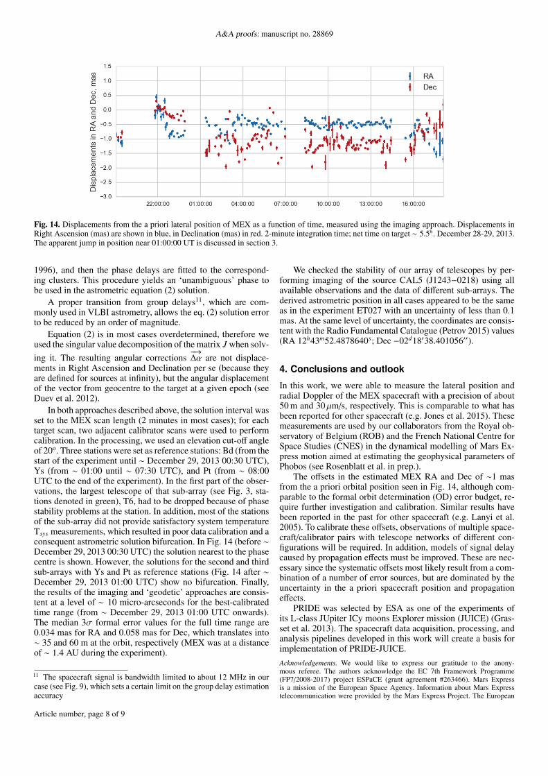
Fig. 14. Displacements from the a priori lateral position of MEX as a function of time, measured using the imaging approach. Displacements inRight Ascension (mas) are shown in blue, in Declination (mas) in red. 2-minute integration time; net time on target ∼ 5.5h. December 28-29, 2013.The apparent jump in position near 01:00:00 UT is discussed in section 3.

1996), and then the phase delays are fitted to the correspond-ing clusters. This procedure yields an ‘unambiguous’ phase tobe used in the astrometric equation (2) solution.

A proper transition from group delays11, which are com-monly used in VLBI astrometry, allows the eq. (2) solution errorto be reduced by an order of magnitude.

Equation (2) is in most cases overdetermined, therefore weused the singular value decomposition of the matrix J when solv-ing it. The resulting angular corrections

−→∆α are not displace-

ments in Right Ascension and Declination per se (because theyare defined for sources at infinity), but the angular displacementof the vector from geocentre to the target at a given epoch (seeDuev et al. 2012).

In both approaches described above, the solution interval wasset to the MEX scan length (2 minutes in most cases); for eachtarget scan, two adjacent calibrator scans were used to performcalibration. In the processing, we used an elevation cut-off angleof 20o. Three stations were set as reference stations: Bd (from thestart of the experiment until ∼ December 29, 2013 00:30 UTC),Ys (from ∼ 01:00 until ∼ 07:30 UTC), and Pt (from ∼ 08:00UTC to the end of the experiment). In the first part of the obser-vations, the largest telescope of that sub-array (see Fig. 3, sta-tions denoted in green), T6, had to be dropped because of phasestability problems at the station. In addition, most of the stationsof the sub-array did not provide satisfactory system temperatureTsys measurements, which resulted in poor data calibration and aconsequent astrometric solution bifurcation. In Fig. 14 (before ∼December 29, 2013 00:30 UTC) the solution nearest to the phasecentre is shown. However, the solutions for the second and thirdsub-arrays with Ys and Pt as reference stations (Fig. 14 after ∼December 29, 2013 01:00 UTC) show no bifurcation. Finally,the results of the imaging and ‘geodetic’ approaches are consis-tent at a level of ∼ 10 micro-arcseconds for the best-calibratedtime range (from ∼ December 29, 2013 01:00 UTC onwards).The median 3σ formal error values for the full time range are0.034 mas for RA and 0.058 mas for Dec, which translates into∼ 35 and 60 m at the orbit, respectively (MEX was at a distanceof ∼ 1.4 AU during the experiment).

11 The spacecraft signal is bandwidth limited to about 12 MHz in ourcase (see Fig. 9), which sets a certain limit on the group delay estimationaccuracy

We checked the stability of our array of telescopes by per-forming imaging of the source CAL5 (J1243−0218) using allavailable observations and the data of different sub-arrays. Thederived astrometric position in all cases appeared to be the sameas in the experiment ET027 with an uncertainty of less than 0.1mas. At the same level of uncertainty, the coordinates are consis-tent with the Radio Fundamental Catalogue (Petrov 2015) values(RA 12h43m52.4878640s; Dec −02d18′38.401056′′).

4. Conclusions and outlook

In this work, we were able to measure the lateral position andradial Doppler of the MEX spacecraft with a precision of about50 m and 30 µm/s, respectively. This is comparable to what hasbeen reported for other spacecraft (e.g. Jones et al. 2015). Thesemeasurements are used by our collaborators from the Royal ob-servatory of Belgium (ROB) and the French National Centre forSpace Studies (CNES) in the dynamical modelling of Mars Ex-press motion aimed at estimating the geophysical parameters ofPhobos (see Rosenblatt et al. in prep.).

The offsets in the estimated MEX RA and Dec of ∼1 masfrom the a priori orbital position seen in Fig. 14, although com-parable to the formal orbit determination (OD) error budget, re-quire further investigation and calibration. Similar results havebeen reported in the past for other spacecraft (e.g. Lanyi et al.2005). To calibrate these offsets, observations of multiple space-craft/calibrator pairs with telescope networks of different con-figurations will be required. In addition, models of signal delaycaused by propagation effects must be improved. These are nec-essary since the systematic offsets most likely result from a com-bination of a number of error sources, but are dominated by theuncertainty in the a priori spacecraft position and propagationeffects.

PRIDE was selected by ESA as one of the experiments ofits L-class JUpiter ICy moons Explorer mission (JUICE) (Gras-set et al. 2013). The spacecraft data acquisition, processing, andanalysis pipelines developed in this work will create a basis forimplementation of PRIDE-JUICE.

Acknowledgements. We would like to express our gratitude to the anony-mous referee. The authors acknowledge the EC 7th Framework Programme(FP7/2008-2017) project ESPaCE (grant agreement #263466). Mars Expressis a mission of the European Space Agency. Information about Mars Expresstelecommunication were provided by the Mars Express Project. The European



VLBI Network is a joint facility of independent European, African, Asian, andNorth American radio astronomy institutes. Scientific results from data presentedin this publication are derived from the following EVN project code: GR035.The National Radio Astronomy Observatory is a facility of the National ScienceFoundation operated under cooperative agreement by Associated Universities,Inc. The Australia Telescope Compact Array is part of the Australia TelescopeNational Facility which is funded by the Commonwealth of Australia for opera-tion as a National Facility managed by CSIRO. This study made use of data col-lected through the AuScope initiative. AuScope Ltd is funded under the NationalCollaborative Research Infrastructure Strategy (NCRIS), an Australian Com-monwealth Government Programme. The authors would like to thank the person-nel of the participating stations. R.M. Campbell, A. Keimpema, P. Boven (JIVE),M. Pätzold (University of Cologne), B. Häusler (University of BW Munich),and D. Titov (ESA/ESTEC) provided important support to various componentsof the project. G. Cimó acknowledges the Horizon 2020 project ASTERICS.T. Bocanegra Bahamon acknowledges the NWO–ShAO agreement on collabo-ration in VLBI. J. Kania acknowledges the ASTRON/JIVE Summer Studentshipprogramme. P. Rosenblatt is financially supported by the Belgium PRODEX pro-gram managed by the European Space Agency in collaboration with the BelgianFederal Science Policy Office.

References

Beasley, A. J. & Conway, J. E. 1995, in Astronomical Society of the Pacific Con-ference Series, Vol. 82, Very Long Baseline Interferometry and the VLBA, ed.J. A. Zensus, P. J. Diamond, & P. J. Napier, 327

Budnik, F., Morley, T. A., & MacKenzie, R. A. 2004, in ESA Special Publication,Vol. 548, 18th International Symposium on Space Flight Dynamics, 387

Du, P., Kibbe, W. A., & Lin, S. M. 2006, Bioinformatics, 22, 2059Duev, D. A., Molera Calvés, G., Pogrebenko, S. V., et al. 2012, A&A, 541, A43Duev, D. A., Zakhvatkin, M. V., Stepanyants, V. A., et al. 2015, A&A, 573, A99Ester, M., Kriegel, H.-P., Sander, J., & Xu, X. 1996, in Second International Con-

ference on Knowledge Discovery and Data Mining (KDD-96) (AAAI Press),226–231

Grasset, O., Dougherty, M. K., Coustenis, A., et al. 2013, Planet. Space Sci., 78,1

Greisen, E. W. 2003, Information Handling in Astronomy - Historical Vistas,285, 109

Högbom, J. A. 1974, A&AS, 15, 417Jones, D. L., Folkner, W. M., Jacobson, R. A., et al. 2015, AJ, 149, 28Keimpema, A., Kettenis, M. M., Pogrebenko, S. V., et al. 2015, Experimental

Astronomy, 39, 259Kemball, A. J. & Wieringa, M. H., eds. 2000, MeasurementSet definition, ver.

2.0.Kettenis, M., van Langevelde, H. J., Reynolds, C., & Cotton, B. 2006, in As-

tronomical Society of the Pacific Conference Series, Vol. 351, AstronomicalData Analysis Software and Systems XV, ed. C. Gabriel, C. Arviset, D. Ponz,& S. Enrique, 497

Lanyi, G., Border, J., Benson, J., et al. 2005, Interplanetary Network ProgressReport, 162, 1

Molera Calvés, G. 2012, PhD thesis, Aalto University, Pub. No. 42/2012Molera Calvés, G., Pogrebenko, S. V., Cimò, G., et al. 2014, A&A, 564, A4Pätzold, M., Häusler, B., Tyler, G., et al. 2016, Planetary and Space Science, 127,

44Pätzold, M., Neubauer, F. M., Carone, L., et al. 2004, in ESA Special Publication,

Vol. 1240, Mars Express: the Scientific Payload, ed. A. Wilson & A. Chicarro,141–163

Petrov, L. 2015, Radio Fundamental Catalog, http://astrogeo.org/rfc, ac-cessed: 2015-08-01

Ros, E., Marcaide, J. M., Guirado, J. C., et al. 1999, A&A, 348, 381Shu, F., Petrov, L., Jiang, W., et al. 2016, ArXiv e-prints [arXiv:1605.07036]Traa, J. & Smaragdis, P. 2013, IEEE Signal Processing Letters, 20, 1257Tyler, G. L., Balmino, G., Hinson, D. P., et al. 1992, J. Geophys. Res., 97, 7759Witasse, O., Duxbury, T., Chicarro, A., et al. 2014, Planet. Space Sci., 102, 18

Appendix A: Wrapped Kalman smoother

The wrapper Kalman filter (WKF) is a Kalman filter for whichthe filtered state distribution PWN is represented by a wrappedGaussian (Traa & Smaragdis 2013):

PWN(ϕ | µ, σ2) =1

σ√

2π

∞∑l=−∞

exp[−

(ϕ − (µ + 2πl))2

2σ2

], ϕ ∈ S1

(A.1)

The wrapped Gaussian distribution results from mapping anormally distributed random variable γ ∼ N(µ, σ2), ϕ ∈ R1 ontoa unit circle S1:

ϕ = ψ(γ) = mod(γ + π, 2π) − π (A.2)

The filtering algorithm is summarised below:

Predict :z−t = Azt−1

z−t [1] = ψ(z−t−1[1])

Σ−t = AΣ−t−1AT + Σv

Correct :

Kt =Σ−t BT

BΣ−t BT + σ2w

gt =

1∑l=−1

((ϕt + 2πl) − z−t [1])ηt,l

zt = z−t + Ktgt

Σt = (I − KtB)Σ−t (A.3)

where zt =

[ϕtϕt

]is the system’s state, zt[1] = ϕt, A =

[1 dt0 1

]is the linearised state transition matrix, dt is the time intervalbetween the (t − 1)th and (t)th epochs, Σv is the state covariancematrix, Σt is the state covariance matrix estimate, B = [1 0] isthe observation matrix, σw is the observation variance, I is anidentity matrix, and ηt,l = N(ϕt +2πl | z−t [1], σ2

w)/∑∞

m=−∞N(ϕt +2πm | z−t [1], σ2

w) represents the probability of a replicate.First, the filter is run on the phase data turned ‘backwards’ in

time running from tN to t1, where N is the number of data points.The system state z is initialised as

z0 =

[ϕN0

](A.4)

The output of this filtering procedure at t0 is used as the ini-tial condition for running the Kalman filter ‘forward’ in time.Usually, it is enough to run the filter backward and forward onceto get a robust and reliable result, but if several iterations areneeded, the output of the forward-run filter at tN is used to up-date the initial condition for the backward-run.


http://astrogeo.org/rfc

planetary radio interferometry and doppler …. duev et al.: planetary radio interferometry and...

Documents