*hrvflhqwl¿f methods and data systems calibration and ... · doppler michelson interferometry...

Atmos. Meas. Tech., 6, 1761–1776, 2013www.atmos-meas-tech.net/6/1761/2013/doi:10.5194/amt-6-1761-2013© Author(s) 2013. CC Attribution 3.0 License.

EGU Journal Logos (RGB)

Advances in Geosciences

Open A

ccess

Natural Hazards and Earth System

Sciences

Open A

ccess

Annales Geophysicae

Open A

ccess

Nonlinear Processes in Geophysics

Open A

ccess

Atmospheric Chemistry

and Physics

Open A

ccess

Atmospheric Chemistry

and Physics

Open A

ccess

Discussions

Atmospheric Measurement

TechniquesO

pen Access

Atmospheric Measurement

Techniques

Open A

ccess

Discussions

Biogeosciences

Open A

ccess

Open A

ccess

BiogeosciencesDiscussions

Climate of the Past

Open A

ccess

Open A

ccess

Climate of the Past

Discussions

Earth System Dynamics

Open A

ccess

Open A

ccess

Earth System Dynamics

Discussions

GeoscientificInstrumentation

Methods andData Systems

Open A

ccess

GeoscientificInstrumentation

Methods andData Systems

Open A

ccess

Discussions

GeoscientificModel Development

Open A

ccess

Open A

ccess

GeoscientificModel Development

Discussions

Hydrology and Earth System

Sciences

Open A

ccess

Hydrology and Earth System

Sciences

Open A

ccess

Discussions

Ocean Science

Open A

ccess

Open A

ccess

Ocean ScienceDiscussions

Solid Earth

Open A

ccess

Open A

ccess

Solid EarthDiscussions

The Cryosphere

Open A

ccess

Open A

ccess

The CryosphereDiscussions

Natural Hazards and Earth System

Sciences

Open A

ccess

Discussions

Calibration and validation of the advanced E-Region WindInterferometer

S. K. Kristoffersen1, W. E. Ward1, S. Brown2, and J. R. Drummond3

1Department of Physics, University of New Brunswick, Fredericton, NB, E3B 5A3, Canada2CRESS Space Instrumentation Laboratory CSIL, York University, 4700 Keele St. Toronto, ON, M3J 1P3, Canada3Department of Physics and Atmospheric Science, Dalhousie University, Halifax, NS, B3H 4R2, Canada

Correspondence to:W. E. Ward ([email protected])

Received: 31 October 2012 – Published in Atmos. Meas. Tech. Discuss.: 14 November 2012Revised: 8 March 2013 – Accepted: 31 March 2013 – Published: 23 July 2013

Abstract. The advanced E-Region Wind Interferometer (ER-WIN II) combines the imaging capabilities of a CCD detectorwith the wide field associated with field-widened Michelsoninterferometry. This instrument is capable of simultaneousmulti-directional wind observations for three different air-glow emissions (oxygen green line (O(1S)) at a height of∼ 97 km, thePQ(7) andPP(7) emission lines in the O2(0–1)atmospheric band at∼ 93 km and P1(3) emission line in the(6, 2) hydroxyl Meinel band at∼ 87 km) on a three minutecadence. In each direction, for 45 s measurements for typicalairglow volume emission rates, the instrument is capable ofline-of-sight wind precisions of∼ 1 m s−1 for hydroxyl andO(1S) and∼ 4 m s−1 for O2. This precision is achieved usinga new data analysis algorithm which takes advantage of theimaging capabilities of the CCD detector along with knowl-edge of the instrument phase variation as a function of pixellocation across the detector. This instrument is currently lo-cated in Eureka, Nunavut as part of the Polar EnvironmentAtmospheric Research Laboratory (PEARL) (80◦N, 86◦ W).The details of the physical configuration, the data analysisalgorithm, the measurement calibration and validation of theobservations from December 2008 and January 2009 are de-scribed. Field measurements which demonstrate the capabil-ities of this instrument are presented. To our knowledge, thewind determinations with this instrument are the most accu-rate and have the highest observational cadence for airglowwind observations of this region of the atmosphere and matchthe capabilities of other wind-measuring techniques.

1 Introduction

Interferometric methods have been used for the past thirtyyears to passively observe mesospheric and thermosphericwinds using Doppler shifts in airglow emissions. Progress indetector technologies have led to advances in the observationcapabilities of these instruments by allowing the interferencefringes and/or the scene of interest to be imaged. Apart fromthe Wind Imaging Interferometer (WINDII) on the Upper At-mosphere Research Satellite (Shepherd et al., 1993), publica-tions on working instruments have generally been associatedwith the Fabry–Perot (Aruhliah et al., 2010; Anderson et al.,2012; Shiokawa et al., 2012) and spatial heterodyne spec-troscopy (SHS) techniques (the Doppler Asymmetric SpatialHeterodyne – DASH – of Englert et al., 2012). The successof these instruments demonstrates how incorporating imag-ing capabilities improves the accuracy and temporal resolu-tion over earlier configurations.

In this paper a configuration which implements theseimaging capabilities in combination with a field-widenedMichelson interferometer is described. The approach buildson the foundation developed during work on the WINDIIinstrument. The imaging capability permits simultaneousviewing in multiple directions (as opposed to sequentialviewing in each direction) and allows the fringe profile tobe imaged and analysed on a bin-by-bin basis using new dataanalysis algorithms. The resulting instrument, termed the ad-vanced E-Region Wind Interferometer (ERWIN II), gener-ates simultaneous wind observations in 5 directions (the fourcardinal directions and zenith) at three different heights us-ing three different emissions (the oxygen green line (O(1S))

Published by Copernicus Publications on behalf of the European Geosciences Union.

1762 S. K. Kristoffersen et al.: Calibration and validation of the advanced E-Region Wind Interferometer

at 557.7 nm, thePP(7) andPQ(7) lines in the O2 (0–1) atmo-spheric band at 865.9 and 866.1 nm and the P1(3) emissionline in the OH(6,2) Meinel band at 843.0 nm) every threeminutes. The wind accuracy is∼ 1 m s−1 for all the emis-sions and the precision is∼ 1 m s−1 for the green-line andhydroxyl observations and∼ 4 m s−1 for the O2 observationsfor standard operating conditions.

ERWIN II is based on the E-region wind interferometer(Gault et al., 1996) which was built in the mid-1990s usinga photomultiplier tube as a detector. Winds were obtainedby sequentially viewing different directions. This instrumentwas stationed at Resolute Bay for close to a decade and sev-eral papers on the associated observations published (Fisheret al., 2000, 2002; Bhattacharya and Gerrard, 2010).

In 2005, funding through a Canadian Foundation of Inno-vation grant became available and was used to design andbuild an improved version of the instrument. The interferom-eter and filters from the old version of the instrument wereretained but the optical configuration and imaging detectorswere new. The imaging capability allowed a new data anal-ysis algorithm to be developed, which improved the accu-racy and precision of the instrument. Once completed, ER-WIN II was moved to the Polar Environment AtmosphericResearch Laboratory (PEARL) in Eureka, Nunavut (80◦ N,86◦ W) in February 2008. It operated satisfactorily for threewinters till spring 2011, when some minor issues with its op-eration occurred. These have been fixed and normal opera-tions resumed in the winter of 2012/2013.

This paper is organized as follows. The next two sectionsdeal with concepts and details necessary for understandingthe instrument namely the measurement and instrument con-cept, and a description of the new instrument and its op-eration. In the subsequent section, the data analysis algo-rithms are described. A section on the precision and ac-curacy of these measurements and their validation followsthis. Some initial results along with a comparison with otherwind-measuring instruments and a brief review summary ofthe planned scientific studies with this instrument are thenpresented. The paper finishes with some concluding remarks.

2 Measurement and instrument concept

Doppler shifts in isolated quasi-monochromatic emissionswhen viewed through an ideal Michelson interferometer areseen as changes in the modulation of the interference fringesas a function of path difference. The measured irradianceI (1, λ, x) for an isolated monochromatic emission line hasthe following form:

I (1, λ, x) = I0

(1 + U V cos

(2π

λ1 + x

))+ IB. (1)

HereI0 is the irradiance of the emission alone as measuredat the detector in the absence of interference,1 is the pathdifference of the interferometer,λ is the wavelength of the

emission,x represents small variations in path (typically lessthan λ) that the experimenter can introduce into the inter-ferometer to sample a fringe,U is the relative reduction infringe amplitude due to instrument effects,V is the relativereduction in fringe amplitude due to the finite width of theemission line and the path difference, andIB is the sum ofthe background irradiance of the scene being viewed and de-tector dark count processes.

The phase,θ , of the fringe is defined as2πλ

1. A smallchange in wavelength due to a Doppler shift,λ + δ λ, re-

sults in a change in phase ofδθ =−

(2π

λ2

)1δλ plus a

small correction associated with the dispersion of the glass.For small line-of-sight velocities,vlos, the Doppler shift isδ λ =−λ (vlos/c) with positive line-of-sight velocities corre-sponding to a velocity towards the observer. Hence, the phasechange associated with this Doppler shift is

δθ =2π 1vlos

cλ. (2)

Observation of the phase shift relative to the zero-wind phaseallows the line-of-sight velocity to be derived.

As described in detail elsewhere (Shepherd, 2002),Doppler Michelson interferometry determines winds by de-termining phase shifts in the interference by measuring theirradiance passing through the interferometer at specific pathdifferences and determining the fringe parameters from thesemeasurements. Typically, the interferometer path is varied inphase steps of 90 degrees of phase. The standard 4-point al-gorithm (for ideal conditions: no background or dark count)uses irradiance measurements at four such sequential steps toderive the fringe parameters (irradiance, visibility and phase)as follows:

I0 =I1 + I2 + I3 + I4

4

U V =

[(I1 − I3)

2+ (I4 − I2)

2]1/2

2I0

θa = tan−1(

I4 − I2

I1 − I3

). (3)

In passive remote sensing of winds using airglow emis-sions, the fundamental parameter controlling the measure-ment quality is the instrument throughput,A�, defined asthe product of the area,A, over which the signal is detectedmultiplied by the solid angle at the detector,�, that the sceneof interest subtends. A field-widened Michelson interferome-ter is a configuration of this interferometer which minimizesthe path variation as a function of angle through the inter-ferometer (Shepherd, 2002; details and references pertinentto the following summary can be found in this monograph).Generally the field is collimated through the interferometerso the phase variation as a function of angle through the in-terferometer is projected onto the observed scene. The fieldwidening is achieved by optimally inserting excess glass into

Atmos. Meas. Tech., 6, 1761–1776, 2013 www.atmos-meas-tech.net/6/1761/2013/

S. K. Kristoffersen et al.: Calibration and validation of the advanced E-Region Wind Interferometer 1763

one of the arms of the interferometer and positioning the mir-ror in the other arm at the apparent position of the mirrorof the arm with the excess glass in it so that the conditionswhen the arms are the exactly the same are approximatelyachieved. This configuration eliminates the second-order de-pendence of path as a function of angle and can eliminate thefourth-order dependence for specific mirror positions (Zwickand Shepherd, 1971).

The precision of a wind measurement is basically relatedto how well the sinusoidal variation associated with a varia-tion in path can be discerned relative to the inherent noise as-sociated with that measurement. For a shot-noise-limited ob-servation, a reasonable estimate of accuracy of the phase de-termination is the standard deviation inθ , σθ , which is givenby Ward (1988):

σθ =1

aU V√

I0, (4)

wherea is a constant which depends on the number of stepsused to determine the fringe phase. For the four point mea-surement described abovea =

√2. For the 8-step scans used

for ERWIN II, a = 2.The two fringe-related parameters in this equation are the

net visibility, U V , and√

I0, which is the signal-to-noise ra-tio. In practice, the measurement precision can be increasedby increasing the signal (longer integration times and en-hanced instrument responsivity) or the visibility. The visi-bility is determined by the emission line width, backgroundemissions, the instrument imperfections and the phase vari-ation over the region used to detect the light (essentially theaperture effect discussed by Hilliard and Shepherd, 1966).

Contributions of background or dark signal to the observedirradiance also affect the measurement precision. In terms ofthe above formulation for ideal conditions, this can be ac-commodated by determining effective irradiances and effec-tive visibilities where the effective irradiance isIe

0 = I0 + IBand the effective visibility isU V e =U V (I0/(I0 + IB)). Inthe rest of this paper, for simplicity, expressions will be pro-vided for the ideal conditions (i.e. no dark and no back-ground) with the understanding that for non-ideal conditions,the effective irradiance and visibility can be used without anychange to their form.

The wind accuracy is a function of both the measure-ment precision and knowledge of the phase for a stationarysource, termed here the zero-wind phase. Generally, practi-cal sources for the airglow emissions are not available so thezero-wind phase is determined by using lamps with emis-sion lines at wavelengths close to the airglow emissions andusing nightly averages of the wind in the vertical directionunder the assumption that vertical motions average to a valuesmaller than the precision.

3 Instrument description and operation

ERWIN II differs from the original instrument in that thephotomultiplier tube was replaced by an imaging detector,the optics were modified so that light from the four cardinaldirections and the vertical could be viewed simultaneously,and the interferometer was placed in an air-tight housing toprevent pressure changes associated with weather fronts fromaffecting the phase. The interferometer, airglow emissions,calibration lines and the filters used are the same as ERWINand are described in detail in Gault et al. (1996).

In summary, the interferometer is a three-glass design withthe mirror position controlled using piezoelectric cylindersand a capacitive feedback system. The front face is squarewith sides of 7.62 cm. It was designed to accept a beamwith a 2.5◦ half angle. The interferometer is set to a pathdifference slightly larger than 11 cm and the glass lengthswere chosen so that the interferometer is field widened at allwavelengths and thermally compensated. The specific pathdifference was selected to suppress possible fringes fromthermospheric oxygen green-line emissions, and to ensurethe fringes of the pair of O2 lines and the3 doubled hy-droxyl lines were each in phase. The calibration lines usedare the 557.0 nm krypton line, the 840.8 nm argon line andthe 866.7 nm argon line.

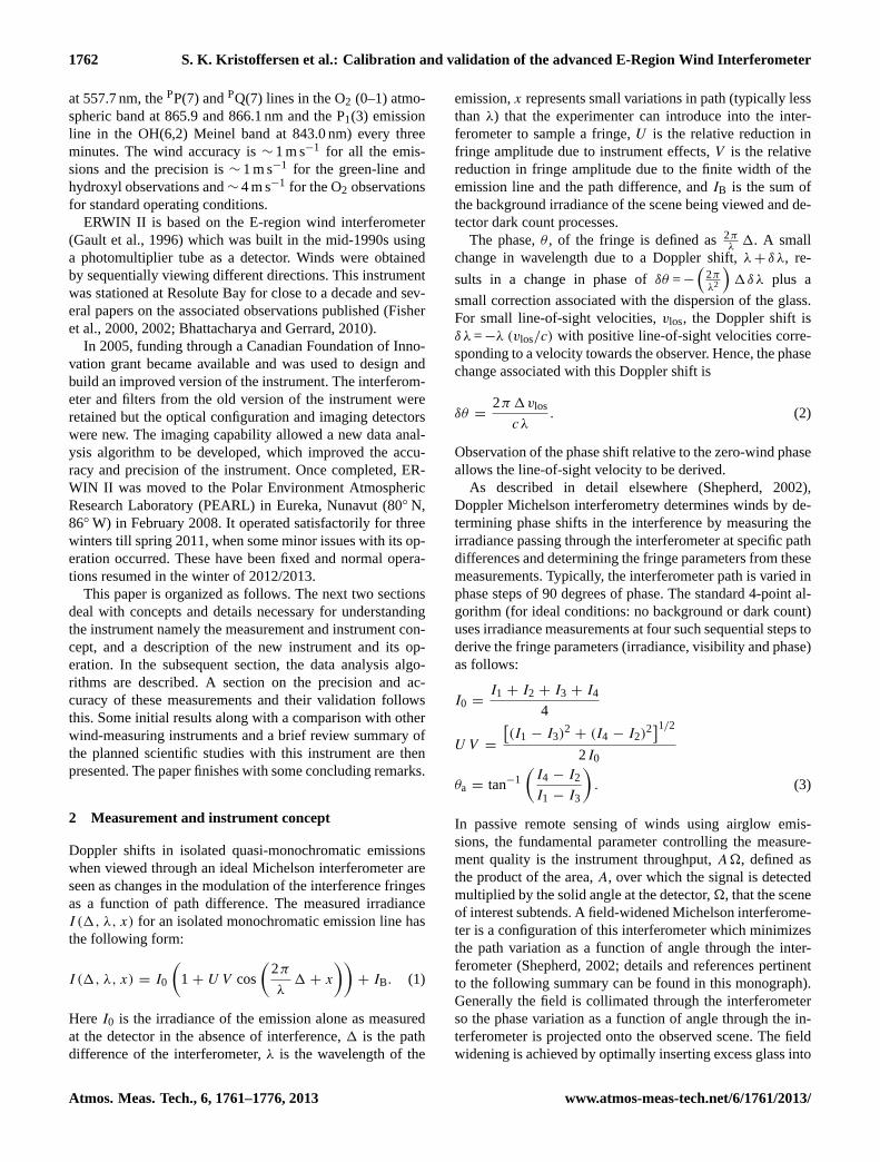
Figure 1 is a schematic view of the mechanical layout ofERWIN II. It shows a cut through the centre of the instru-ment such that two of the cardinal viewing directions and thevertical can be seen (the other viewing directions project outof the plane of the figure). The centres of each cardinal view-ing direction are at an elevation angle of 38.7◦ relative to thehorizontal. Light from the sky from all the viewing directionsis collected and focused on what is termed the quad mirror,where they are combined into a single beam and then passedthrough the interferometer. The interferometer is tilted 1.77◦

horizontally and 1.77◦ vertically relative to the optical axisof the system to ensure that no light was reflected off opti-cal components and recycled back through the system. Theoptical components which collect the light and collimate itthrough the interferometer form what is termed the front tele-scope. After the interferometer, a second optical system –termed the back telescope – directs the light to the filters,where the light is again collimated. Both telescopes are 1 : 1.The camera system then focuses the beam onto the detector.

The calibration lamps are located outside of the Michelsonhousing and are not pictured in the schematic shown in Fig. 1.The lamps are connected to fibre optic cables, which are di-rected at the calibration lamp screen. This screen acts as ashutter; when it is closed, atmospheric measurements cannotbe taken. To take calibration lamp measurements, this shut-ter/screen is closed, and illuminated by the calibration lamps,and thereby acting as a source for the calibration lines.

The quad mirror consists of four trapezoidal mirrorscanted appropriately with a square hole in the middle. Thisserves to redirect light from each direction so that they

www.atmos-meas-tech.net/6/1761/2013/ Atmos. Meas. Tech., 6, 1761–1776, 2013


Fig. 1.Diagram of ERWIN mechanical layout.

combine with the zenith light into a single beam throughthe rest of the optical system. Each of the cardinal directionsviews an irregularly shaped piece of the sky approximately0.0013 steradians at an elevation angle of 38.7◦. Zenith isviewed with a solid angle of 0.0007 steradians. Light fromeach of the cardinal directions is focused onto one of thetrapezoidal facets of the quad mirror using spherical mirrorsand zenith is focused onto the plane of this mirror. The quadmirror is located at the field stop of the front telescope. Thelight from these various viewing directions is passed as col-limated light through the interferometer and then focused us-ing a second telescope and camera onto the detector. The skyfrom each direction is thus focused onto different regions ofthe detector so that each of these five directions is simultane-ously measured. The effective field of view of the instrument

is the same as that allowed through the interferometer – abeam of 2.5◦ half angle.

The camera was built in-house at York University anduses a 512× 512 pixel, back-thinned, low-noise, frame-transfer CCD (E2V Technologies CCD57-10) with an ac-tive area of 6.656× 6.656 mm. The CCD camera is usedwith 16 × 16 binning, resulting in a final image size of35 × 32 bins. It has a quantum efficiency of 0.85 for theO(1S) emission and 0.45 and 0.4 for the O2 and OH emis-sions. This is a significant improvement over the photomul-tiplier tube for which the quantum efficiency was∼ .14,.08 and .06 for the same emissions. An additional advan-tage arises, as noted above, because of the imaging capabil-ity; measurements could be made with enhanced visibilityover the original instrument. The increased sensitivity allowsfor a decrease in the exposure times, while still maintaining



Fig. 2. Green-line background phase (in radians) from 26 Jan-uary 2009. The x- and y-axes represent pixel indices. The blackenedbins represent the borders between the sections of the quad mirror.The top section measures east, the bottom, west, the left, south, theright, north, and the centre zenith.

comparable signal to noise. For ERWIN II the radianceresponse is 1.7672 Rayleigh (counts s)−1 for green line,2.0682 Rayleigh (counts s)−1 for O2 and 1.0627 Rayleigh(counts s)−1 for OH.

Figure 2 illustrates the manner in which the field is im-aged onto the CCD detector. The dark bins indicate wherethe edges of the areas illuminated by the various regions ofthe sky are located. The light from each viewing directionis imaged as follows: the top – east, the bottom – west, theright – north, the left – south, and the centre – zenith. Thebackground colours indicate how the interferometer phase inradians varies across the field and indicate how much vari-ation there is across each region. Variations in phase awayfrom this background along with consideration of the zerowind provide a measure of the Doppler shift in each viewingdirection.

The observation procedure of ERWIN II has been updatedrelative to that described in Gault et al. (1996). Since allviewing directions are now viewed simultaneously, there isno need to cycle through the viewing directions. The basicprocedure is to cycle through the three emission measure-ments in sequence and then after a user specified number ofcycles to perform a set of calibrations. A measurement con-sists of 8 exposures of the detector each at a different valueof the Michelson path. The steps (relative to the referencephase which coincides with the initial mirror position) are setto 0, 90, 180, 270, 270, 180, 90 and 0◦ of phase. These stepsare different for each emission with 360◦ corresponding to aphysical change in path ofλ, the wavelength of the emissionbeing viewed. A calibration consists of measurements (againone for each emission) using the calibration lamps and a darkmeasurement. Initially, a calibration was undertaken after ev-ery eight emission scans, but later this was changed to every

Fig. 3. Schematic of the viewing geometry of ERWIN II. Thisshows three fields of view. The other two are orthogonal to the planeof the page.

set of emission scans to provide better precision for deter-mining the interferometer drift. Overall, this results in a setof observations (wind determinations for 5 directions and allthree emissions) approximately every 3 min. ERWIN takesmeasurements as long as the solar elevation is less than 0◦.

The observing geometry is illustrated in Fig. 3. All threeemission layers are shown schematically and occur roughlyat nominal heights of 97, 93 and 87 km for the O(1S), O2and OH emissions, respectively. Thus, by cycling throughthe different emissions, information on various heights in themesopause region is acquired. The azimuthal viewing direc-tions are at an elevation angle ofα = 38.7◦ from the horizon-tal. Based on this observing geometry, the∼ 5◦ lateral crosssection of each beam, and a mean height of 90 km and a nom-inal vertical scale of∼ 5 km for the half width of the airglowlayer, the volume of atmosphere sampled by ERWIN II is∼ 5 km in the vertical and 5km by 6km in the horizontal. (Itwill not be sensitive to vertical scales less than approximatelyhalf the thickness of the airglow layer –∼ 5 km). Since windsare determined by observing Doppler shifts in the emissionfrequencies, the observed, line-of-sight winds are combina-tions of the horizontal and vertical winds (save for the zenithline-of-sight winds, which observe vertical winds).

The meridional wind,v, is determined using the differenceof the line-of-sight north and south winds

v =

(V LOS

S − V LOSN

)2 cosα

, (5)

where

V LOSN = −v cosα + w sinα (6)

V LOSS = v cosα + w sinα. (7)

Herew is the vertical component of the wind andα is theviewing angle of the azimuthal look directions relative to thehorizontal (cos(α) ≈ 0.7804 and sin(α) ≈ 0.6252).



Similarly, the zonal wind,u, can be determined using theeast and west line-of-sight winds,

u =

(V LOS

W − V LOSE

)2 cosα

. (8)

The vertical winds can also be obtained using several differ-ent approaches. The most precise and accurate is to use thezenith line-of-sight winds

w = V LOSZ . (9)

The vertical winds can be also be determined indirectly usingthe cardinal direction line-of-sight winds,

w =V LOS

N + V LOSS

2 sinα=

V LOSE + V LOS

W

2 sinα. (10)

In theory, this provides the means to check the internal con-sistency of the wind determinations, but only for longer tem-poral scales. In practice, the effects of gravity waves of scalesof the same order as the distance between the viewing points(∼ 250 km) in the airglow layer will result in oppositely di-rected fields of view measuring winds that differ as a re-sult of the aliasing of wind variations associated with thesewaves. This means that these comparisons can only be un-dertaken for longer term averages for which the spatial scalesare significantly larger than 250 km. At the same time theseshorter term differences between opposing fields of view al-low observations of gravity wave effects to be undertaken,given confidence in the instrument calibration. This will bedescribed in detail in a forthcoming paper.

4 Data analysis procedure

The essential issue for wind measurements is distinguishingthe phase increments,δ θ , associated with Doppler shifts inthe emission of interest from the phase associated with otherfactors. In general, the observed phase is a combination of thephase associated with the instrument configuration as mani-fested for the emission of interest (motionless) plus a shiftassociated with atmospheric motion of the source region be-ing viewed. In practice, for imaging applications, the phaseassociated with the instrument configuration can be separatedinto three terms:

– θB(i, j): a term associated with the phase variationacross the field as a function of angle through the inter-ferometer (or pixel location (i, j ) on the detector) rel-ative to the phase associated with rays passing at nor-mal incidence through the interferometer (backgroundphase). This variation is illustrated in Fig. 2.

– θT(t) : a term giving the thermal-drift phase of the inter-ferometer relative to the phase observed at a particulartime (thermal-drift term).

– θ0: a term identifying the phase that a motionless sourcewould have (zero-wind phase).

Hence, the measured phase,θa, can be expressed as a func-tion of time,t , and location on the field as

θa(i, j, t) = θB(i, j) + θ0 + θT(t) + δ θ(t). (11)

This formulation of the phase assumes that the back-ground phase stays constant (generally satisfied for carefullymaintained interferometers) and temporal variations can betracked with a single phase parameter, the thermal drift,which is only a function of time.

In theory, the zero-wind phase should be easy to determinesince it only requires a stationary source for the emission ofinterest. In practice, however, this is difficult to achieve sinceportable sources for the airglow emissions are unavailableand the atmosphere is generally in motion. As with otherground-based wind instruments, a daily average of the ob-served vertical wind is used to determine this parameter.In the case of ERWIN II this average is measured usingthe quadrant looking vertical. For measurements at Eureka,where close to 24 h each day is observed, this determinationis expected to be a good measure of the actual zero wind;all periods of tidal motions are covered during this time pe-riod, variations associated with gravity waves are expectedto average to zero, vertical winds associated with planetarywaves are of the order of cm s−1 and mean vertical winds aresmall (an ascent or descent of 10 km day−1 corresponds to avertical velocity of 0.11 m s−1).

For ERWIN II the background phase determination wasmore difficult than expected. Initially, it was thought thephase variation associated with the reference emissionswould be suitable to use since they were within a fewAngstroms of the emission of interest. However, it was foundthat use of such a background resulted in phase variations of∼ 10 m s−1 across several of the quadrants when daily av-erages of the winds were calculated. This effect is thoughtto be due to differences between the calibration optics andmain optics which result in the light distribution across theaperture of each system being different and resulting in adifferent weighting of any residual path variations in the in-terferometer. Instead, the background phase which was usedwas determined using wind observations from a period whenit was known to be cloudy (this phase variation is illustratedin Fig. 2 for the green line). Light from the sky was suit-ably scattered so that all directions gave the same Dopplershift. Daily averages of this wind for the oxygen green-lineand hydroxyl observations using this background are pre-sented in Fig. 4. The resulting wind variations are minimalin each quadrant and the mean wind in each quadrant pro-vides a measure of the mean wind for the day. Details of theanalysis which lead to this choice of background wind arecontained in Kristoffersen (2012).

Although the analysis approach described in Gault etal. (1996) could be implemented for ERWIN II by integrating



the signal in each quadrant and treating each quadrant asa single detector, a new bin-by-bin least-mean-squares ap-proach similar to that implemented in Ward (1988) was pre-ferred. The latter approach was more precise since it avoidsany visibility reduction that occurs as a result of the inte-gration over the phase in each quadrant, and it allows binscontaminated by stars or cosmic ray hits to be eliminated. Inaddition, a rigorous determination of the wind error can beundertaken.

For this approach, a non-linear least-mean-squares analy-sis using the Levenberg Marquardt method (as described inPress et al., 2007) is implemented. The variation in photonsdetected per integration time for a step during thek-th 8-pointscan is modelled according to the following equation:

I (i, j, tk, s) = I0 (tk) (1 + U V (tk) cos(δ θ (tk) + θI (i, j, tk, s))) , (12)

where the parameters being solved for areI0(tk), the num-ber of photons detected per integration time for a step inthe absence of interference,U V (tk), the net visibility, andδ θ(tk), the phase variation associated with the wind. Heretk is the time of thek-th scan. To ensure that the variationin angles being determined is small, all the known phasesassociated with a particular bin are added together so thatθI (i, j, tk, s) = θB(i, j) + θ0 + θT (tk) + (1θs), where(1θs)

is the step size increment associated with mirror step of in-dex s (expressed as a phase angle).

The merit function is

χ2=

N∑s=1

(Is(i, j, tk, s) − y (I (i, j, tk, s) ; al)

)2

σ 2s (i, j, tk, s)

, (13)

where

y (I (i, j, tk, s) ; al) = al(1) (1 + al(2) cos(al(3) + θI (i, j, tk, s)))

al =(I0l (tk) , U Vl (tk) , δ θl (tk)

).

Is(i, j, tk, s) is the number of photons detected for stepss,bin (i, j ) and scank, andσ 2

s (i, j, tk, s) is the associated vari-ance (estimated as shot noise).l is the iteration index, soy (I (i, j, tk, s) ; al) is the number of photons detected de-termined using the constants determined on thel-th iteration.θI (i, j, tk, s) with 1θs = 0 is used to seed the first iteration ofthis method. Typically, only a few iterations are needed forconvergence to a solution.

In practice, there are two approaches used to determine thezero wind and thermal-drift phase: one using the calibrationlamp phase determinations (the standard procedure) and theother when the calibration lamp phase is not available (as oc-curred for the OH emission when the lamp malfunctioned).For the standard procedure, the calibration phase was deter-mined on a regular basis throughout the night by calculatingthe average Michelson phase over the full field of the cali-bration lamp using the same 8-point scan as for the airglowobservations. The resulting time series of calibration phaseis interpolated using cubic splines to the airglow observation

times to provide the variation in the thermal-drift phase. Therelative airglow phase throughout the observation period isthen calculated using the non-linear approach with the zero-wind phase set to zero. The actual zero-wind phase then pro-vides an offset to this relative phase and is determined usingthe mean of the zenith over the entire day. The winds are de-termined by shifting the relative airglow phase by the zero-wind phase and using Eq. (2) to convert the phase to velocity.

If the calibration lamps are not available, then the zenithmeasurements can be used to estimate the phase associatedwith the thermal drift and zero wind. In this case, the anal-ysis approach as described above is undertaken but with thethermal-drift and zero-wind terms set to zero. For each im-age, the phase for the vertical view is then taken as an esti-mate of the sum of these two terms and subtracted off the fourother quadrants. The disadvantage of this approach is that thevertical wind cannot be determined and phase variations as-sociated with vertical winds are mixed into the phase deter-minations for each of the cardinal directions. This reducesthe precision and accuracy of the radial wind determination.Nevertheless, the meridional and zonal wind determinationsare unaffected by the lack of an independent zero-wind de-termination since they are determined through a difference inradial wind determinations in opposite directions, and hencethe zero-wind contribution to the two directions is eliminated(see Eqs. 5 and 8).

There are several advantages associated with the standardapproach described above. This algorithm can be run forfewer than the 8 steps comprising a typical scan. Because thesteps are in phase multiples of 90◦ and all phases steps arerepeated twice, anomalous numbers of photons detected at aparticular step can be identified by comparing photon num-bers observed for steps of the same phase and examining thesums of photon numbers for steps which are 180◦ apart. Ifone or two steps with anomalous numbers of detected pho-tons are identified in a scan, they are eliminated from thephase determination, thereby reducing the likelihood of out-liers. In addition, there are∼ 150 bins used for wind deter-minations in each of the cardinal directions and∼ 80 binsfor the vertical. As a result, any additional outliers beyondthree standard deviations of the mean wind phase in each ofthe quadrants can be identified and are then eliminated andthe standard error associated with the wind determination foreach quadrant calculated. Implementation of these checks re-sults in a robust statistical framework for the wind determi-nations with this instrument.

5 Measurement validation

In this section, results which verify the precision and accu-racy of the ERWIN II instrument are presented. Crucial isan accurate determination of the background phase variationacross the field, the thermal drift and the zero wind. Eachof these aspects of the wind determination contributes to the



Fig. 4. An image of the daily averaged wind image (m s−1) for the green-line and OH observations on 26 January 2009, using the 28 Jan-uary 2009 phase average for the background phase. The averages are calculated on a bin-by-bin basis. The sector averages of these imagesprovide the daily mean winds in each direction. The uniformity of each sector and the fact that opposite sectors are of similar magnitude butopposite sign indicates that the phase background is not introducing systematic errors into the wind determinations.

measurement precision and accuracy. Evaluation of the mea-surement quality in terms of these aspects is possible becauseof redundancies in the approach and tests which were un-dertaken to investigate specific aspects of the measurementapproach.

As noted above, the background phase was determined us-ing observations taken on 28 January 2009 during a periodwhen it was cloudy so that the directional asymmetry in theDoppler shifts would be negligible as a result of scatteringin the clouds. During the eight hours of observations usedto determine this phase variation,∼ 160 measurements weretaken. The background phase was determined by taking theaverage of these measurements. For the fringe parametersassociated with these measurements, the standard deviationof the wind determination for each bin on each scan was∼ 15 m s−1 so that would be the standard error for the back-ground phase determination was∼ 1.1 m s−1 for each bin.Since winds are determined by averaging the phases deter-mined on a bin-by-bin basis in each sector, this error makesa negligible contribution to the measurement precision.

Equally important is determining whether there are anysystematic errors in the background determination. This isimportant since the winds in opposite directions are deter-mined relative to the background phase so errors in thebackground phase would result in systematic errors in thesewinds. Figure 4 shows the daily average wind image mea-sured on 26 January 2009 for the oxygen green-line and hy-droxyl observations. Shown for each emission is the dailyaverage of each bin in the image. The average of each sec-tor gives the mean radial wind in each direction for this day.Two things of particular note are the uniformity of the windsin each quadrant and that opposite quadrants are close to thesame magnitude but oppositely signed. The uniformity indi-cates that the background phase has been effectively removedfrom the wind determinations since the gradient associated

with the angular dependence of the background phase is notobserved. The fact that the winds in opposing directions areconsistent with what would be expected geometrically indi-cates that errors in the background phase determination areminimal and do not result in systematic errors in the radialwind determinations. The wind is defined as positive towardsthe instrument, so the observation of a positive (negative)wind in one sector would correspond to a wind of the op-posite sign in the opposite quadrant.

This self-consistency of ERWIN II is further demonstratedby considering the averages of these sectors for several days,shown in Table 1. Since the winds in opposing directionsshould have the same magnitude but opposite sign, the sumof these values should be zero. The table provides the val-ues of the average daily phase for each of the four sectorscorresponding to the cardinal directions for three days inJanuary 2009 for the hydroxyl and green-line observations.The means for each sector over the three days is calculated(4th column) and then the sum of the phases of oppositesectors determined. Since the winds in opposing directionsshould have the same magnitude, but opposite sign, the sumof these values should be close to zero, as observed. On av-erage, the difference is of the order of 1 m s−1. This furthervalidates that the background is suitable for the wind deter-minations and at most a systematic error of 1 m s−1 is intro-duced into the radial wind observations. The use of this phasebackground has been checked for the subsequent years and itis a stable feature of the interferometer.

These results also demonstrate that, on average, the ther-mal drift is being calculated properly. Since the thermal driftwould be a constant value added to the phase for every bin,at a given time, this value would have the same sign foreach section. This would result in an addition of the thermal-drift terms, rather than the cancellation of the winds, as isobserved.



Table 1. Comparisons of the mean differences of the daily averages of the opposite sight directions for the green-line and OH emissionsusing the 28 January 2009 background phase.

Green line – 28 January background

Mean phase (degrees) Difference

23 Jan 25 Jan 26 Jan Mean Difference (m s−1)

Bottom – West −2.2689 −5.2311 −4.3201 −3.9419 −0.3266 −1.4216Top – East 2.183 5.5978 3.0596 3.6154Left – South −2.3606 −0.424 1.2777 −0.5042 −0.0115 −0.0416Right – North 3.5065 −0.1719 −1.8564 0.4927

OH – 28 January background

Mean phase (degrees) Difference

23 Jan 25 Jan 26 Jan Mean Difference (m s−1)

Bottom – West −1.885 −2.6528 −2.9221 −2.4866 0.1948 0.8563Top – East 1.9366 3.4263 2.6872 2.6814Left – South −2.5153 −2.7731 −0.8938 −2.0626 0.2177 0.9477Right – North 3.4492 2.3319 1.0542 2.2804

Fig. 5. (a)Plot of green-line-emission zenith phase (blue dots) and the calibration phase (red dots) on 26 January 2009. The measurementuncertainty of the phase measurements is smaller than the size of the dots in this plot.(b) Plot of the difference between the zenith phaseand the calibration phase interpolated using cubic splines to the times of the atmospheric observations. The zenith observations includegeophysical variability. The time is UTC.

Depending on the thermal stability of the instrument short-term measurement errors can also be introduced if the ther-mal drift is not followed with sufficient precision. As de-scribed earlier, initially calibration phase measurements weretaken on a slower cadence than the measurements. For thefirst two years of observations, one scan of the calibrationlamps was taken for every eight scans of the atmosphericemissions. For the third year (March 2010 to March 2011)this was increased to a calibration every measurement scanof the atmospheric emissions.

Figure 5 gives an indication of the precision of thethermal-drift determination. Figure 5a (upper panel) shows atime series of the green-line zenith phase (blue points) alongwith the phase determined with the calibration lamp (red dots– corrected with the zero-wind offset so that both time serieshave the same daily average). On this figure the uncertaintiesin the phase determinations are smaller than the diameter ofthe dots in the plots. The two phase determinations followeach other closely.



Figure 5b (lower panel) is a time series of the differencebetween the observed zenith phase and the calibration phaseinterpolated using cubic splines to the times of the atmo-spheric observations. In this figure the measurement preci-sion is close to the size of the dots. The standard deviationof the difference is 1.02◦ or 4.5 m s−1. This number includesgeophysical variability (vertical winds, volume emission ratevariations) and Schott noise and hence is not a clean mea-sure of the uncertainty introduced through the thermal-driftcalibrations.

To explore this aspect of the measurement in more detail,an experiment which included frequent calibration measure-ments was performed (a calibration measurement was takenafter every atmospheric measurement). The resulting calibra-tion phase time series was compared to one constructed bysampling this time series at a the same rate as other typicaldays and then interpolating (using cubic splines) these mea-surements to the times of the original time series. This pro-cess duplicated the thermal phase determinations associatedwith the atmospheric measurements

Figure 6 shows the result of this experiment. The phaseerror in the cubic spline is never more than a degree, andthe standard deviation of the phase error over the duration ofthis experiment is 0.328◦ (1.43 m s−1). This is significantlysmaller than the standard deviation of the difference of thecalibration phase and the zenith emission phase, which was1.02◦ (4.5 m s−1). This demonstrates that the errors associ-ated with the cubic spline are acceptably small compared tothe other errors and geophysical noise. This uncertainty isreduced for observations with the more frequent calibrationcadence.

Using the value of “a” appropriate for the 8-step scan,and substituting appropriately in Eqs. (2) and (4), the fol-lowing expression for the standard deviation (which we useas a measure of the wind precision) is obtained:

σw =cλ

4π 1eff U V√

I. (14)

Hereσw is the error in m s−1, 1eff is the effective path dif-ference,U V is the visibility, I is the observed number ofphotons detected per integration time per step in the absenceof interference effects,c is the speed of light andλ is thewavelength of the emission. The wind standard deviation isinversely proportional toU V , the path difference and thesquare root ofI . Comparison of the estimated variance usingthis formula to the observed variance provides an indicationof how closely the observations conditions during individualscans match the assumptions associated with the derivationof this formula (namely that the source radiance and visibil-ity remain constant during a scan).

This is illustrated in Fig. 7, which provides time series ofthe actual standard error and the standard error estimated us-ing Eq. (12) (calculated as a variance for each bin in the sec-tor using Eq. (14) and then averaged in the same way as the

Fig. 6. Plot of the error in the cubic spline interpolation for thegreen-line calibration lamp sampled every∼ 30 min relative to theoriginal time series and interpolated to the times of the original timeseries. Every 8th point of the original time series is used for the in-terpolation (the error for these points is identically zero).The datawere recorded on 20 March 2010.

actual standard error is calculated), the signal (in analogueto digital units – ADU) and visibility for the north sector on22 December 2008. The variability in both data sets is dueto variations in the airglow volume emission rate (primar-ily) and visibility during that day. The expected decrease inthe standard error when the signal increases (and vice versa)is evident in the upper two plots. It is striking that the twomeasures follow each other so closely since this indicatesthat intensity and visibility variations during individual scansare generally insignificant. If they are a factor then the stan-dard error would be significantly larger than the estimatedprecision.

Figure 8 shows time series of the standard error for allfour cardinal direction sectors for 26 January 2009. For thisdate, some twilight was present in the afternoon centred at∼ 17:00 UTC. The increase in the standard error in the vicin-ity of this time is the expected result of increases in the back-ground relative to the airglow volume emission rate (see dis-cussion at the end of Sect. 2). The time series of all four sec-tors follow each other well. The daily average of the green-line standard error for the zenith section is 1.91 m s−1, andthat for all of the cardinal directions is 1.22 m s−1. The dailyaverage of the precision based on the visibility and intensityof the green-line emission for zenith is 1.88 m s−1, and thatfor the cardinal directions is 1.24 m s−1. The values for zenithare greater than for the cardinal directions because of geo-metrical considerations. The effective layer thickness (andhence irradiance) is greater by 1/cos(α), whereα is the in-clination angle relative to zenith (hereα = 51.3◦). The irra-diance during this day was lower on average, so these val-ues are slightly higher than the typical precision of thesemeasurements.



Fig. 7.Comparison of the standard error (blue points) for northern sector compared to theσw (red points). Below this panel the correspondingdetected signal (in ADU, middle panel) and visibility (lower panel) as a function of time for the same day are shown. Decreases in the standarderror are mainly associated with increases in the signal as expected given the visibility stays roughly constant throughout the day.

Fig. 8. Standard errors for each of the cardinal direction sectors ofthe CCD on from 26 January 2009.

Plots of the winds provide a final, and satisfactory, checkthat the results are accurate. Meridional winds from 23 Jan-uary 2009 for green line and hydroxyl calculated in sev-eral different ways are shown in Fig. 9. The meridional,north direction and south direction winds are calculated us-ing Eqs. (5)–(7), respectively. The time series designated“without subtracting zenith” is a time series of the wind

determined from the northern sector without zenith sub-tracted. The meridional winds are reasonable, and indi-cate that there was a significant semi-diurnal tidal variationpresent. The manner in which this wind is determined rendersit independent of vertical wind and thermal drift. Althoughperturbations due to gravity waves will result in small devi-ations from the true large-scale meridional wind above thestation, to good approximation this time series can be con-sidered a good measure of the true meridional wind. Issueswith thermal-drift, zero-wind or background phase will resultin the meridional winds determined solely from the north orsouth directions deviating significantly from this time series.

All the green-line winds agree well with each other. Thenorth and south winds, which are the winds determined fromthe respective sectors with the zenith phase subtracted offto remove any thermal drift, follow the meridional windvery closely. This demonstrates that the winds viewed fromthe different directions are self-consistent. The fourth windplotted on this figure is the north wind without the zenithphase subtracted. Since this also fits the meridional wind veryclosely, it demonstrates that the thermal drift has been effec-tively removed from the wind phase for observations withthis emission.

The OH observations are taken during the time when theassociated calibration lamp was not working. As with thegreen-line observations, the north and south winds follow themeridional wind closely. In contrast, the north wind withoutzenith subtracted deviates significantly from the other winds.



Fig. 9.Time series of meridional winds (m s−1) from 23 January 2009 for the green-line(a) and hydroxyl emission(b) observations showingthe consistency of the observations in the north and south directions when thermal drift and zero wind are appropriately accounted for andthe problems – green points – in(b) when they are not. The standard errors of these observations are approximately the size of the points inthe figure. Detailed discussion is in the text.

As expected, since there are no calibration measurementsto provide thermal-drift information, omission of the zenithphase results in winds which exhibit significant systematicerrors.

Since the contribution of the thermal-drift variance to thewind observations is∼ 2.85 m2 s−2 for the time when thelonger cadence calibration period was implemented, it is pos-sible to use the zenith phase to examine the vertical wind(for the shorter cadence calibration period this will be evenmore feasible). While the exploration of this possibility willrequire careful analysis, an indication that this is plausiblecomes from a comparison (see Fig. 10) between the verticalwind determined using the zenith phase (blue dots) and thevertical wind determined using Eq. (10) (black dots). Bothof these methods provide similar results on the larger tempo-ral scales. Over the day, the vertical wind is modulated sinu-soidally by a few m s−1. This could be due to a diurnal tide,although since this day was during the 2009 major strato-spheric warming, other dynamical effects could be present(Manney et al., 2009). The variance in the directly measuredvertical wind is 30.9 m2 s−2, which is significantly greaterthan the contribution associated with the thermal-drift deter-mination. The variance in the indirect determination of thevertical wind is 89.4 m2 s−2. This calculation however alsoincludes contributions from horizontal motions due to grav-ity waves and other high wave number phenomena. Furtheranalysis of the vertical winds will be undertaken in the fu-ture to determine whether definitive geophysical results arepossible.

In this section, the various factors affecting the precisionand accuracy of the ERWIN II wind results have been dis-cussed and results demonstrating the internal consistency ofthe winds presented. The main factors affecting the mea-surement precision are the uncertainties associated with

Fig. 10. Green-line vertical wind (m s−1) 25 January 2009 as di-rectly observed (blue dots) and as calculated using the north, south,east and west winds (black dots) according to Eq. (10).

the Schott noise and the thermal-drift determination. Forthe observations with the low cadence calibration measure-ments the net variance is∼ 4 m2 s−2 (i.e. (1.22)2 + (1.43)2)for the green-line and OH observations and∼ 19 m2 s−2

(i.e. (4.0)2 + (1.43)2) for the O2 observations. These valuesdepend on the manner in which the thermal drift varies andfor the observations taken with the high cadence calibrationswill be close to the Schott noise values alone. The O2 valuesare significantly greater than the other two emissions becauseits irradiance is significantly smaller. For all the emissions,the precision is dependent on the detected number of pho-tons/step and visibility. There are occasions when the airglowvolume emission rate is close to a factor of four greater thanthat for the days used in this paper to validate the instrument.



On these days the standard error will be less than 1 m s−1 forobservations during which the calibration cadence was high.

The measurement accuracy for radial winds is determinedby the uncertainty in the background phase determination(< 1 m s−1) and uncertainties in the zero-wind determina-tion. Based on the arguments presented in Sect. 4, this is ex-pected to be less that 1 m s−1 also. Hence, for the best obser-vation procedure (high cadence calibrations), the precisionand accuracy are both∼ 1 m s−1.

6 Discussion

Comparisons between the capabilities of ERWIN II and otheroptical wind measuring instruments are not straightforward.Although theoretical comparisons based on throughput con-siderations have been undertaken (see Shepherd, 2002), fewpapers have discussed the precision and accuracy of a tech-nique in practice in as much detail and as clearly as has beenundertaken in this paper. In part this is because a standardfor comparison has not been developed, in part because theprecision is dependent on the integration time (i.e. amountof light collected), instrument aperture and field of view, andthermal stability, and lastly in part because clear identifica-tion of the zero wind is difficult in practice. Instead, estimatesof the measurement precision tend to be embedded in mea-surement papers using the particular technique in question.Since most techniques use some sort of average of the verti-cal wind over a night to estimate the true zero, unless thereare other systematic errors, one can assume that the measure-ment accuracies are similar. As a result the measurement pre-cision (taken as the standard deviation of the velocity deter-mination) and the integration time needed for the measure-ment as quoted in the literature are the only pragmatic meansto use in comparing different instruments.

For ERWIN II, five velocity measurements at a precisionof 1 m s−1 in 45 s are observed for an airglow brightnessslightly below average. In a recent paper on multiple orderFabry–Perot wind observations (Shiokawa et al., 2012) (sim-ilar to the observation technique used by Makela et al., 2011and Meriwether et al., 2011) random errors ranging from 2 to13 m s−1 are quoted for a single wind observation with an ex-posure time of 60 s. Assuming that observing conditions inthe middle of this range correspond to those for ERWIN II, itwould take this instrument∼ 5 min to observe the same fivevelocities with a precision of∼ 7 m s−1.

The Scanning Doppler Interferometer (SCANDI) de-scribed by Arulia et al. (2010) is used for all-sky auroralimaging by using multiple fringes. They note that it takes∼ 7–8 min to obtain a 25-sector wind measurement for theseemissions, which are about an order of magnitude greaterin brightness than they are at mid-latitudes (i.e. airglow aswith ERWIN-II). For measurements on 8 March 2007 anuncertainty of 15 m s−1 is quoted. Assuming that the mea-surement uncertainty scales roughly as the reciprocal of the

square root of the brightness, the uncertainty in these mea-surements would be∼ 45 m s−1 (i.e. 15 m s−1

×√

10) for abrightness an order of magnitude less than that observed. Ifthis was reduced to a 5-sector measurement by combining theobserved irradiances, then the precision would be∼ 20 m s−1

(i.e. 45/√

5) for a∼ 7 min measurement.The DASH instrument (Englert et al., 2007) was recently

used in field measurements at a mid-latitude site to compareresults to a Fabry–Perot interferometer (Englert et al., 2012).For this comparison, 5 min integrations were taken and theoxygen red line was observed. Uncertainties at the one sigmalevel ranged from∼ 5 to 15 m s−1 based on the plots in thispaper. It would take> 25 min to achieve the 5-measurementcycle of ERWIN II at a precision≥ 5 m s−1.

This comparison indicates that the precision and measure-ment cadence achieved by ERWIN II is significantly superiorto any others reported in the literature. Of these, the multipleorder Fabry–Perot of Shiokawa et al. (2012) comes closest tothe ERWIN II performance. Even with this instrument (againassuming the uncertainty scales with number of photons de-tected per step as described above) it would require an inte-gration time of 225 min (5 min× 72) to achieve the 1 m s−1

precision that ERWIN II achieves. These comparisons are notdefinitive since the instruments described in these papers donot necessarily represent their optimal configuration. How-ever, the advantage shown by ERWIN II is unlikely to bematched by minor changes in the configurations of these in-struments. At this time it provides the most precise and rapidairglow wind measurements in the world.

Rockets, lidar and radar are three other techniques used tomeasure winds in the mesopause region. Although compar-isons with the precision of the wind measurements associ-ated with these techniques are undertaken below, other im-portant aspects of the dynamical fields are measured usingthese instruments (for example temperature and density withlidar and diffusion with rockets and radar). In addition, theirmeasurements may be more extensive that those undertakenwith ERWIN II (i.e. inclusion of day/night observations or agreater height range and vertical resolution).

Rockets provide short-term wind observations in this re-gion with a wind precision of 5–10 m s−1, a temporal res-olution of 3 s and a height resolution of∼ 1 km over about10 min (Larson, 2002; Chu et al., 2007 and referencestherein). She et al. (2003) state that their sodium lidar hasa vertical resolution of 2 km and measures winds between81 and 107 km. The wind precision is∼ 1.5 m s−1 at thepeak of the layer (∼ 91 km) and∼ 15 m s−1 at the upperand lower bounds of their measurements for a 1 h integra-tion during night. In a comparison between radar (middleand upper atmosphere – MU – radar (meteor mode)) andFabry–Perot winds observed over Shigaraki, Japan, Fujii etal. (2004) quote uncertainties of 2–5 m s−1 for 1 km resolu-tion and 30 min integrations at∼ 93 km, which is close tothe height of maximum meteor trail detection. Radial winduncertainties associated with a meteor radar in a paper by



Fig. 11.Time series of the zonal and meridional winds for all three emissions on 22 December 2008. It is interesting to note that larger scalevariations first show up in the green-line winds, followed by O2 and then OH. This is expected for upward propagating tides for which thephase front propagates downward. Standard errors for each wind measurement are smaller than the dots in the figure for green line and OHand about the size of the dot for O2.

Frank et al. (2005) which compares lidar winds to meteorradar winds are quoted as being a few m s−1 for (time/height)bins of (60 min/4 km). For the lidar used in this study, vec-tor winds were obtained with∼ 1 m s−1 precision between85 and 100 km with a 12 min cycle and vertical resolution of∼ 1 km (Liu and Gardener, 2005).

As discussed by Franke et al. (2005) and Fujii et al. (2004),the geometries of the observing conditions associated withthe various wind measuring instruments are different. Theyare sensitive to different temporal and spatial scales, so themeasurement variances are affected differently by geophysi-cal variability. ERWIN II views a brightness-weighted wind,so as noted in Sect. 3 it can be considered to provide windsfor a volume of atmosphere of∼ 5 km in the vertical and5 km by 6 km in the horizontal In contrast, the lidar collectsinformation from volumes with heights of 1 km and a diam-eter of∼ 50 m and the meteor radar collects information pervelocity measurement from a volume 4 km thick and 200 kmdiameter (Franke et al., 2005). The sampling area of the MUradar per velocity measurement is from a volume 1 km thickand 200 km in diameter. Based on the height range and ver-tical resolution of the best of these various instruments, thelidar achieves 15 velocity measurements at a 1 m s−1 preci-sion in 12 min, and the MU radar achieves 40 velocity mea-surements at a 3–5 m s−1 precision (recent upgrades to theMU radar may have enhanced its capabilities). With a vec-tor wind measurement every 45 s at a precision of∼ 1 m s−1,ERWIN II has similar capabilities to these instruments. For a

cycle through the three emissions, winds at nominal heightsof 7, 93 and 97 km at the four cardinal directions and thevertical are obtained every three minutes at a precision equalto or better than these instruments and at a measurement ca-dence faster than either of these instruments. On the otherhand, these instruments provide better spatial resolution thanERWIN II (especially in the vertical) since the observationvolumes associated with each measurement are smaller.

Some indication of the capabilities of ERWIN II for sci-entific purposes is shown in Fig. 11. Here time series ofthe meridional and zonal winds observed by ERWIN II on22 December 2008 for all three emissions are presented.As expected for larger scale upward propagating waves, thephase progression is downward with the green-line windsleading, followed by O2 and then OH. Standard errors foreach wind measurement are smaller than the dots in the fig-ure for green line and OH and about the size of the dot forO2. The smaller scale variations are real and provide the op-portunity to investigate the wind fields at these heights onsmaller temporal scales than previously possible. Given thatERWIN II simultaneously provides observations of the rela-tive brightness of the airglow emissions that it observes, therelationship between the winds and airglow can be exploredin detail. Of particular interest is the investigation of grav-ity waves and the associated vertical velocities and airglowvariations.

The PEARL facility, where ERWIN II is currently located,houses three other instruments which take measurements in



the upper mesosphere and lower thermosphere. These in-clude an All-Sky Imager (ASI) (observes OH, Na, O(1S),O(1D) and N+

2 ), a spectral airglow temperature imager(SATI: O2, OH; Sargoytchev et al., 2004; Shepherd et al.,2010), and a meteor radar (Manson et al., 2009). The mea-surement cadences of the ASI and SATI are of the order ofminutes, and the meteor radar provides an hourly verticalprofile of horizontal wind in the mesopause region. Inter-comparisons between simultaneous observations taken withthese instruments open up many possibilities for new sci-entific studies. Initial comparisons between ERWIN II andthe meteor radar show them to be in reasonable agreement(a comparison which deals with the complexities of the ob-servational filters of each instrument will be published sep-arately). The dynamical signatures of specific events (suchas stratospheric warming), wave signatures and the relation-ships between temperature, wind and emission rate over abroad range of scales are topics which this research station isespecially capable of investigating.

7 Conclusions

The construction of ERWIN II and the completion of newdata analysis algorithms have resulted in a powerful new ca-pability for investigating the dynamics of the mesopause re-gion. The most important physical changes to the instrumentinclude the addition of a quad mirror to the ERWIN opticaltrain so that multiple viewing directions can be simultane-ously observed and the inclusion of a CCD camera so thateach of these directions can be simultaneously imaged. Thenew data analysis algorithm takes advantage of the imagingcapabilities of the new instrument to provide a more pre-cise and better monitored wind and volume emission rateobservations.

In this paper the capabilities of this instrument havebeen thoroughly discussed. For the standard observation se-quence, wind measurements have a precision and accuracyof ∼ 1 m s−1 and a 3 min observation cadence which incor-porates observations in five viewing directions for each ofthree different emissions. This accuracy, precision and ob-serving cadence was shown to be the best to date for opticalinstruments which use airglow to measure winds. Compar-isons with superior radar and lidar systems indicate that ER-WIN II wind observations are among the best in the world.

New science is anticipated with this instrument. On itsown, vertical winds and relationships between the wind com-ponents and airglow volume emission rate can be investi-gated at temporal scales previously unachievable. Of partic-ular interest in this respect is the investigation of the relation-ships between these variables in gravity waves and tides, andthe investigation of the velocity spectra at these heights.

The installation of ERWIN II at PEARL, along with sev-eral other instruments which observe temperature, airglowand wind in the mesopause region, establishes a unique

and potent capability both amongst Arctic observatories andworldwide. These instruments include a SATI, an All-SkyImager and a meteor radar. Together they support the inves-tigation of the spatial and temporal variability of the tem-perature, wind and airglow on temporal scales of minutesto months and spatial scales from kilometres to hundreds ofkilometres.

Acknowledgements.The Canadian Network for the Detectionof Atmospheric Change (CANDAC)/PEARL funding partnersare as follows: the Arctic Research Infrastructure Fund, AtlanticInnovation Fund/Nova Scotia Research Innovation Trust, CanadianFoundation for Climate and Atmospheric Science, CanadianFoundation for Innovation, Canadian Space Agency, EnvironmentCanada, Government of Canada International Polar Year, NaturalSciences and Engineering Research Council, Ontario InnovationTrust, Ontario Research Fund, Indian and Northern Affairs Canada,and the Polar Continental Shelf Program. Funds from the CanadianFoundation of Innovation were essential for the construction ofthe ERWIN II instrument. Research support through grants fromthe Natural Sciences and Engineering Council (NSERC), researchfunding from the Canadian Foundation for Climate and Atmo-spheric Science (CFCAS), and support from the CREATE programof NSERC as well as the University of New Brunswick andYork University are acknowledged. Financial support for StephenBrown was provided through the CRESS Space InstrumentationLaboratory (CSIL) at York University. Brian Solheim and GordonShepherd are also thanked for their support of the design andconstruction of ERWIN II.

Edited by: A. Stoffelen

References

Anderson, C., Conde, M., and McHarg, M. G.: Neutral thermo-spheric dynamics observed with two scanning Doppler imagers:1. Monostatic and bistatic winds, J. Geophys. Res., 117, A03304,doi:10.1029/2011JA017041, 2012.

Aruliah, A. L., Griffin, E. M., Yiu, H.-C. I., McWhirter, I., and Char-alambous, A.: SCANDI – an all-sky Doppler imager for studiesof thermospheric spatial structure, Ann. Geophys., 28, 549–567,doi:10.5194/angeo-28-549-2010, 2010.

Bhattacharya, Y. and Gerrard, A. J.: Wintertime mesopause re-gion vertical winds from Resolute Bay, J. Geophys. Res., 115,D00N07,doi:10.1029/2010JD014113, 2010.

Chu, Y. H., Su, C. L., Larsen, M. F., and Chao, C. K.: Firstmeasurements of neutral wind and turbulence in the meso-sphere and lower thermosphere over Taiwan with a chem-ical release experiment, J. Geophys. Res., 112, A02301,doi:10.1029/2005JA011560, 2007.

Englert, C. R., Babcock, D. D., and Harlander, J. M.: DopplerAsymmetric Spatial Heterodyne Spectroscopy (DASH): conceptand experimental demonstration, Appl. Optics, 46, 7297–7307,2007.


http://dx.doi.org/10.1029/2011JA017041

http://dx.doi.org/10.5194/angeo-28-549-2010

http://dx.doi.org/10.1029/2010JD014113

http://dx.doi.org/10.1029/2005JA011560


Englert, C. R., Harlander, J. M., Brown, C. M., Meriwether, J.W., Makela, J. J., Castelaz, M., Emmert, J. T., Drob, D. P., andMarr, K. D.: Coincident thermospheric wind measurements usingground-based Doppler Asymmetric Spatial Heterodyne (DASH)and Fabry–Perot Interferometer (FPI) instruments, J. Atmos.Sol.-Terr. Phy., 86, 92–98, 2012.

Fisher, G. M., Killeen, T. L., Wu, Q., Reeves, J. M., Hays, P. B.,Gault, W. A., Brown, S., and Shepherd, G. G.: Polar cap meso-sphere wind observations: Comparisons of simultaneous mea-surements with a Fabry–Perot interferometer and a field-widenedMichelson interferometer, Appl. Optics, 39, 4284–4291, 2000.

Fisher, G. M., Niciejewski, R. J., Killeen, T. L., Gault, W. A., Shep-herd, G. G., Brown, S., and Wu, Q.: Twelve-hour tides in the win-ter northern polar mesosphere and lower thermosphere, J. Geo-phys. Res., 107, 1211,doi:10.1029/2001JA000294, 2002.

Franke, S. J., Chu, X., Liu, A. Z., and Hocking, W. K.: Comparisonof meteor radar and Na Doppler lidar measurements of windsin the mesopause region above Maui, Hawaii, J. Geophys. Res.,110, D09S02,doi:10.1029/2003JD004486, 2005.

Fujii, J., Nakamura, T., Tsuda, T., and Shiokawa, K.: Comparisonof winds measured by MU radar and Fabry–Perot interferometerand effect of OI5577 airglow height variations, J. Atmos. Sol.-Terr. Phy., 66, 573–583, 2004.

Gault, W. A., Brown, S., Moise, A., Liang, D., Sellar, G., Shepherd,G. G., and Wimperis, J.: ERWIN: An E region wind interferom-eter, Appl. Optics, 35, 2913–2922,doi:10.1364/AO.35.002913,1996.

Hilliard, R. L. and Shepherd, G. G.: Wide-Angle Michelson Inter-ferometer for measuring Doppler line widths, J. Opt. Soc. Am.,56, 362–369, 1966.

Kristoffersen, S. K.: The E-Region Wind Interferometer (ERWIN):Description of the Least Mean Squares Data Analysis Routine,Wind Results and Comparisons with the Meteor Radar, Univer-sity of New Brunswick, Fredericton, NB, Canada, 2012.

Larsen, M. F.: Winds and shears in the mesosphere andlower thermosphere: Results from four decades of chem-ical release wind measurements, J. Geophys. Res., 107,doi:10.1029/2001JA000218, 2002.

Liu, A. Z. and Gardner, C. S.: Vertical heat and constituenttransport in the mesopause region by dissipating grav-ity waves at Maui, Hawaii (20.7◦ N), and Starfire OpticalRange, New Mexico (35◦ N), J. Geophys. Res., 110, D09S13,doi:10.1029/2004JD004965, 2005.

Makela, J. J., Meriwether, J. W., Huang, Y., and Sherwood, P. J.:Simulation and analysis of a multi-order imaging Fabry–Perotinterferometer for the study of thermospheric winds and temper-atures, Appl. Optics, 50, 4403–4416, 2011.

Manney, G. L., Schwartz, M. J., Kruger, K., Santee, M. L., Paw-son, S., Lee, J. N., Daffer, W. H., Fuller, R. A., and Livesey,N. J.: Aura Microwave Limb Sounder observations of dy-namics and transport during the record-breaking 2009 Arcticstratospheric major warming, Geophys. Res. Lett., 36, L12815,doi:10.1029/2009GL038586, 2009.

Manson, A. H., Meek, C. E., Chshyolkova, T., Xu, X., Aso, T.,Drummond, J. R., Hall, C. M., Hocking, W. K., Jacobi, Ch., Tsut-sumi, M., and Ward, W. E.: Arctic tidal characteristics at Eureka(80◦ N, 86◦ W) and Svalbard (78◦ N, 16◦ E) for 2006/07: sea-sonal and longitudinal variations, migrating and non-migratingtides, Ann. Geophys., 27, 1153–1173,doi:10.5194/angeo-27-1153-2009, 2009.

Meriwether, J. W., Makela, J. J., Huang, Y., Fisher, D. J., Bu-riti, R. A., Medeiros, A. F., and Takahashi, H.: Climatology ofthe nighttime equatorial thermospheric winds and temperaturesover Brazil near solar minimum, J. Geophys. Res., 116, A04322,doi:10.1029/2011JA016477, 2011.

Press, W. H., Teukolsky, S. A., Vetterline, W. T., and Flannery, B. P.:Numerical Recipes The Art of Scientific Computing, 3rd Edn.,Cambridge University Press, Cambridge, 2007.

Sargoytchev, S. I., Brown, S., Solheim, B. H., Cho, Y.-M., Shep-herd, G. G., and Lopez-Gonzalez, M. J.: Spectral airglow tem-perature imager SATI: a ground-based instrument for the moni-toring of mesosphere temperature, Appl. Optics, 43, 5712–5721,2004.

She, C. Y., Sherman, J., Yuan, T., Williams, B. P., Arnold, K., Kawa-hara, T. D., Li, T., Xu, L. F., Vance, J. D., Acott, P., and Krueger,D. A.: The first 80-hour continuous lidar campaign for simulta-neous observation of mesopause region temperature and wind,Geophys. Res. Lett., 30, 1319,doi:10.1029/2002GL016412,2003.

Shepherd, G. G.: Spectral Imaging of the Atmosphere, ElsevierAcademic Press, London, UK, 2002.

Shepherd, G. G., Thuillier, G., Gault, W. A., Solheim, B. H., Her-som, C., Alunni, J. M., Brun, J.-F., Charlot, P., Cogger, L. L.,Desaulniers, D.-L., Evans, W. F. J., Gattingert, R. L., Girod, F.,Harvie, D., Hum, R. H., Kendall, D. J. W., Llewellyn, E. J.,Lowe, R. P., Ohrt, J., Pasternak, F., Peillet, O., Powell, I., Ro-chon, Y., Ward, W. E., Weins, R. H., and Wimperis, J.: WINDII,the wind imaging interferometer on the Upper Atmosphere Re-search Satellite, J. Geophys. Res., 98, 10725–10750, 1993.

Shepherd, M. G., Cho, Y.-M., Shepherd, G. G., Ward, W.E., and Drummond, J. R.: Mesospheric Temperature andAtomic Oxygen Response during the January 2009 Ma-jor Stratospheric Warming, J. Geophys. Res., 115, A07318,doi:10.1029/2009JA015172, 2010.

Shiokawa, K., Otsuka, Y., Oyama, S., Nozawa, S., Satoh, M.,Katoh, Y., Hamaguchi, Y., and Yamamoto, Y.: Developmentof low-cost sky-scanning Fabry–Perot interferometers for air-glow and auroral studies, Earth Planets Space, 64, 1033–1046,doi:10.5047/eps.2012.05.004, 2012.

Ward, W. E.: Design and Implementation of a Wide Angle Michel-son Interferometer to Observe Thermospheric Winds, Ph.D. The-sis, York University, Toronto, Ont, Canada, 1988.

Zwick, H. H. and Shepherd, G. G.: Defocusing a Wind-AngleMichelson Interferometer, Appl. Optics, 10, 2569–2571, 1971.


http://dx.doi.org/10.1029/2001JA000294

http://dx.doi.org/10.1029/2003JD004486

http://dx.doi.org/10.1364/AO.35.002913

http://dx.doi.org/10.1029/2001JA000218

http://dx.doi.org/10.1029/2004JD004965

http://dx.doi.org/10.1029/2009GL038586



http://dx.doi.org/10.1029/2011JA016477

http://dx.doi.org/10.1029/2002GL016412

http://dx.doi.org/10.1029/2009JA015172

http://dx.doi.org/10.5047/eps.2012.05.004

*hrvflhqwl¿f methods and data systems calibration and ... · doppler michelson interferometry...

Documents