performance evaluation of various image de-noising … evaluation of various image de-noising...

Published by World Academic Press, World Academic Union

ISSN 1746-7659, England, UKJournal of Information and Computing Science

Vol. 8, No. 1, 2013, pp. 013-026

Performance Evaluation of various Image De-noising Techniques

Gurmeet Kaur 1 and Jagroop Singh2 1 Depatment of Electronics and Communication, Rayat & Bahra College of Engineering and Nanotechnology

for Women, Hoshiarpur, Punjab,India

2 Depatment of Electronics and Communication, DAV Institute of Engineering and Technology, Jalandhar, Punjab, India

(Received July 10, 2012, accepted December 24, 2012)

Abstract. The process of removing noise from the original image is still a demanding problem for researchers. There have been several algorithms and each has its assumptions, merits, and demerits. The prime focus of this paper is related to the pre processing of an image before it can be used in applications. The pre processing is done by de-noising of images. In order to achieve these de-noising algorithms, filtering approach and wavelet based approach are used and performs their comparative study. Different noises such as Gaussian noise, salt and pepper noise, speckle noise are used. The wavelet based approach has been proved to be the best in de-noising images corrupted with Gaussian noise, salt and pepper noise and speckle noise A quantitative measure of comparison is provided by the parameters like Peak signal to noise ratio, Root mean square error, Entropy and Correlation of the image.

Keywords: Gaussian noise, Salt & Pepper noise, Speckle noise, Average filter, Wiener filter, Gaussian Filter, Median filter, Wavelet transform.

1. Introduction An image is a two dimensional function f(x, y), where x and y are plane coordinates, and the amplitude

of f at any pair of coordinates (x, y) is called the gray level or intensity of the image at that point. Digital images consist of a finite number of elements where each element has a particular location and value. These elements are called picture elements, image elements and pixels. There are two types of images i.e. grayscale image and RGB image. Gray scale image has one channel and RGB image has three channels i.e. red, green and blue. Image noise is unwanted fluctuations.There are various types of image noises present in the image like gaussian noise, salt & pepper noise, speckle noise, shot noise, white noise[1]. There are various noise reduction techniques are used for removing the noise. Most of the standard algorithms use to de-noise the noisy image and perform the individual filtering process. The result is generally reduced the noise level. But the image is either blurred or over smoothed due to losses like edges or lines. Noise reduction is used to remove the noise without losing much detail contained in an image[2]. To achieve this goal, we use the mathematical function known as the wavelet transform to localize an image into different frequency components or useful sub-bands and effectively reduce the noise in the sub-bands.into different frequency components or useful sub-bands and effectively reduce the noise in the sub-bands.

1.1. Gaussian Filter Gaussian filters are designed to give no overshoot to a step function input while minimizing the rise and

fall time. This behavior of Gaussian filter causes minimum group delay. Mathematically, a Gaussian filter modifies the input signal by convolving with a Gaussian function; The Gaussian filter is usually used as a smoothing filter. The output of the Gaussian filter at the moment is the average of the input values [3].

1.2. Wiener Filter It is used to reduce disturbance (noise) present in a signal by comparison with an estimation of the desired noiseless signal. The design of the Wiener filter is of different approach. The Wiener filtering is a linear

Gurmeet Kaur et.al.: Performance Evaluation of various Image De-noising Techniques

JIC email for contribution: [email protected]

14

estimation of the original image [4]. The approach is based on a stochastic framework. Wiener filters are characterized by the following:

1. Assumption: signal and (additive) noise are stationary linear with known spectral characteristics 2. Requirement: the filter must be physically realizable or casual system. 3. Performance criterion: minimum MMSE[5]

1.3. Average Filter

Mean filter, or average filter is windowed filter of linear class, that smoothes signal (image). The filter works as low-pass one. The basic idea behind filter is for any element of the signal (image) take an average across its neighbourhood. To understand how that is made in practice, let us start with window idea.The Average (mean) filter smooths image data, thus eliminating noise [6]. This filter performs spatial filtering on each individual pixel in an image using the grey level values in a square or rectangular window surrounding each pixel[5].

For example: a1 a2a3 a4 a5 a6 3x3 filter window a7 a8 a9 The average filter computes the sum of all pixels in the filter window and then divides the sum by the number of pixels in the filter window: Filtered pixel = (a1 + a2 + a3 + a4 ... + a9) / 9

1.4. Median Filter

A median filter belongs to the class of nonlinear filters unlike the Average filter. The median filter also follows the moving window principle similar to the Average filter. Median filtering is effective to remove ‘salt and pepper’ type noise. The median is calculated by first sorting all the pixel values from the window into numerical order, and then replacing the pixel being considered with the middle (median) pixel value.

Table1: Concept of Median filtering

123 125 126 130 140

122 124 126 127 135

118 120 150 125 134

119 115 119 123 133

111 116 110 120 130

Neighborhood values: 115,119,120,123,124,125,126,127,150 Median value: 124 The central pixel value of 150 in the 3×3 window shown in Table 1 is rather unrepresentative of the surrounding pixels and is replaced with the median value of 124. The median is more robust compared to the mean. Thus, a single very unrepresentative pixel in a neighborhood will not affect the median value significantly. Since the median value must actually be the value of one of the pixels in the neighborhood, the median filter does not create new unrealistic pixel values when the filter straddles an edge. For this reason the median filter is much better at preserving sharp edges than the mean filter. These advantages aid median filters in de-noising uniform noise as well from an image [19].

1.5. Image Noise

Journal of Information and Computing Science, Vol. 8 (2013) No. 1, pp 013-026

JIC email for subscription: [email protected]

15

The sources of noise in digital images arise during image acquisition and/or transmission. Unavoidable shot

noise of an ideal photon detector [10].!The performance of imaging sensors are affected by a variety of

factors during acquisition, such as

1. Environmental conditions during the acquisition

2. Light levels (low light conditions require high gain amplification).

3. Sensor temperature (higher temp implies more amplification noise)

Depending on the specific noise source, there are different types of noises

• Gaussian noise

• Salt-and-pepper noise

• Speckle noise

1.5.1 Gaussian noise Gaussian noise is a noise that has its PDF equal to that of the normal distribution, which is also known as the Gaussian distribution. Gaussian noise is most commonly known as additive white Gaussian noise. Gaussian noise is properly defined as the noise with a Gaussian amplitude distribution. Labeling Gaussian noise as 'white' describes the correlation of the noise. It is necessary to use the term "white Gaussian noise" to be precise[7][15]. 1.5.2 Salt-and-pepper noise Salt and pepper noise is a noise seen on images. It represents itself as randomly occurring white and black dots. An effective filter for this type of noise involves the usage of a median filter. Salt and pepper noise creeps into images in situations where quick transients, such as faulty switching, take place[9].

1.5.3 Speckle noise

Speckle noise is caused by signals from elementary scatterers, the gravity-capillary ripples, and manifests as a pedestal image.Several different methods are used to eliminate speckle noise, based upon different mathematical models of the phenomenon. One method, for example, employs multiple-look processing[14][16]. A second method involves using adaptive and non-adaptive filters on the signal processing. Such filtering also eliminates actual image information as well, in particular high-frequency information, and the applicability of filtering and the choice of filter type involves tradeoffs. Adaptive speckle filtering is better at preserving edges and detail in high-texture areas (such as forests or urban areas)[8][22]. Non-adaptive filtering is simpler to implement, and requires less computational power.There are two forms of non-adaptive speckle filtering: one based on the mean and one based upon the median (within a given rectangular area of pixels in the image). The latter is better at preserving edges whilst eliminating noise spikes, than the former is[11].

2. Wavelet Transform

Wavelets are mathematical functions that cut up data into different frequency components, and then study each component with a resolution matched to its scale. They have advantages over traditional Fourier methods in analyzing physical situations where the signal contains discontinuities and sharp spikes[20]. Wavelets were developed independently in the fields of mathematics, quantum physics, electrical engineering, and seismic geology. Interchanges between these fields during the last ten years have led to many new wavelet applications such as image compression, turbulence, human vision, radar, and earthquake prediction[12][18]. A wavelet transform is the representation of a function by wavelets. The wavelets are scaled and translated copies of a mother wavelet. Wavelet analysis represents the next logical step: a windowing technique with variable-sized regions. Wavelet analysis allows the use of long time intervals where we want more precise low-frequency information, and shorter regions where we want high frequency



16

information.Wavelet transforms are classified into discrete wavelet transforms (DWTs) and continuous wavelet transforms (CWTs). Both DWT and CWT are continuous-time (analog) transforms. They can be used to represent continuous-time (analog) signals. CWTs operate over every possible scale and translation whereas DWTs use a specific subset of scale and translation values or representation grid[13].

3. Algorithm 3.1 Algorithm for Peak Signal to Noise Ratio (PSNR) Step 1- Difference of noisy image and noiseless image is calculated using imsubract Command. Step 2- Size of the matrix obtains in step 1 is calculated. Step 3- Each of the pixels in the matrix obtained in step is squared. Step 4- Sum of all the pixels in the matrix obtained in step 3 is calculated. Step 5- (MSE) is obtained by taking the ratio of value obtained in step 4 to the value obtained in the step 2 Step 6- (RMSE) is calculated by taking square root to the value obtained in step 5. Step7- Dividing 255 with RMSE, taking 1og base 10 and multiplying with 20 gives the value of PSNR. 3.2 Algorithm for Correlation of Coefficient (Coc) Step1- Mean of the noiseless image and noisy image are calculated. Step2- Mean of the noiseless image is subtracted from each of the pixel in the noiseless image resulting in a matrix. Step3- Similarly the mean of noisy image is subtracted from each of the pixels in the noise image resulting in a matrix. Step 4- Values obtained in step 2 and step 3 are multiplied. Step 5- Sum of all the elements in the matrix obtained in step 4 is calculated. Step 6- Square of all the elements of the matrix obtained in step 2 is calculated and sum of this squared matrix is determined. Step 7- Similarly square of all the elements of the matrix obtained in step 3 is calculated and sum of the elements of this squared matrix is also determined. Step 8- Values obtained in step 6 and step 7 are multiplied and its square root is taken. Step 9- Ratio of the value obtained in step 5 to the value obtained in step 8 is calculated.

3.3 Algorithm for Root Mean Square Error (RMSE) Step 1- Difference of noisy image and noiseless image is calculated using imsubract command. Step 2- Size of the matrix obtains in step 1 is calculated. Step 3- Each of the pixels in the matrix obtained in step is squared. Step 4- Sum of all the pixels in the matrix obtained in step 3 is calculated. Step 5- (MSE) is obtained by taking the ratio of value obtained in step 4 to the value obtained in the step 2. Step 6- (RMSE) is calculated by taking square root to the value obtained in step 5.

3.4 Algorithm for filter selection Step 1- Noiseless image are given as input. Step 2- Noisy image are then given as input. Step 3- Noisy image is filtered by the entire filters i.e. Gaussian, Average, Wiener, Median and Wavelet filter with respect to the noiseless image. Step 4- The statistical parameters are calculated for the filtered image obtained from filtering Step5-Finally we get sets of statistical parameters each set corresponding to 1 filter.

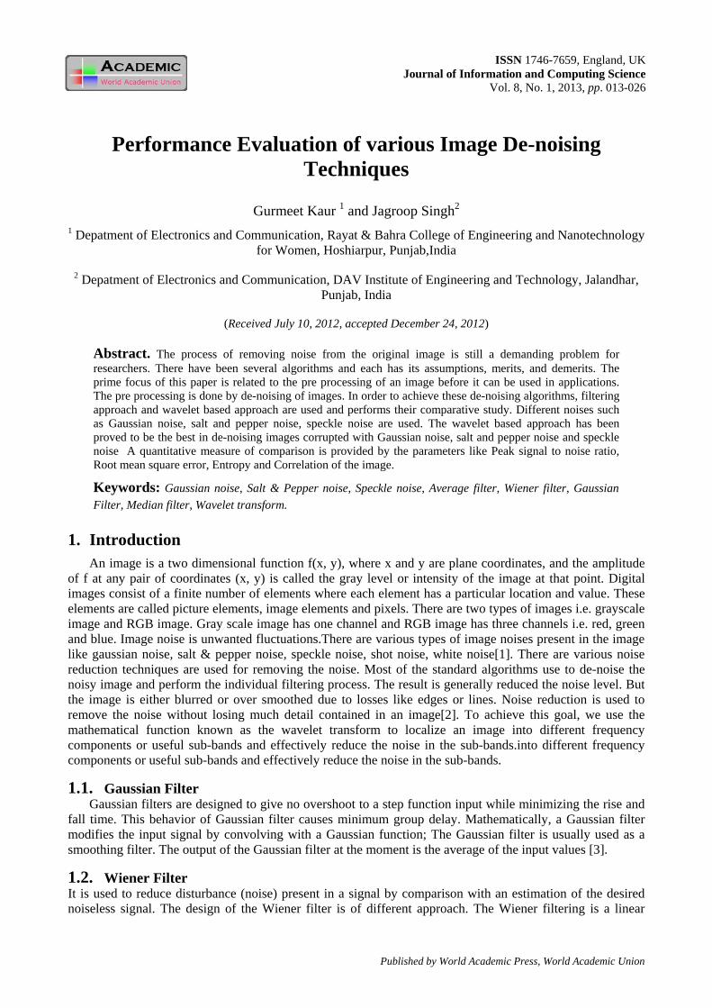
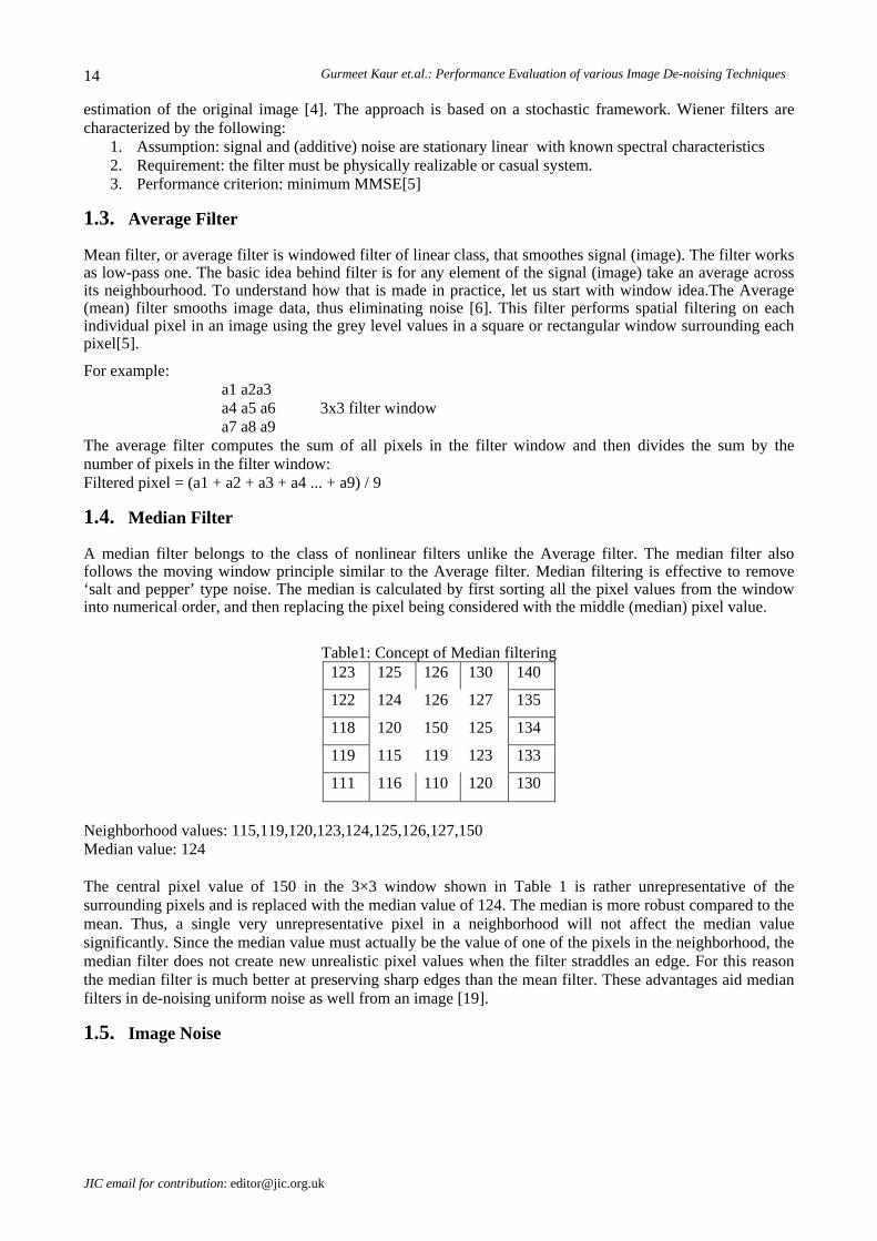
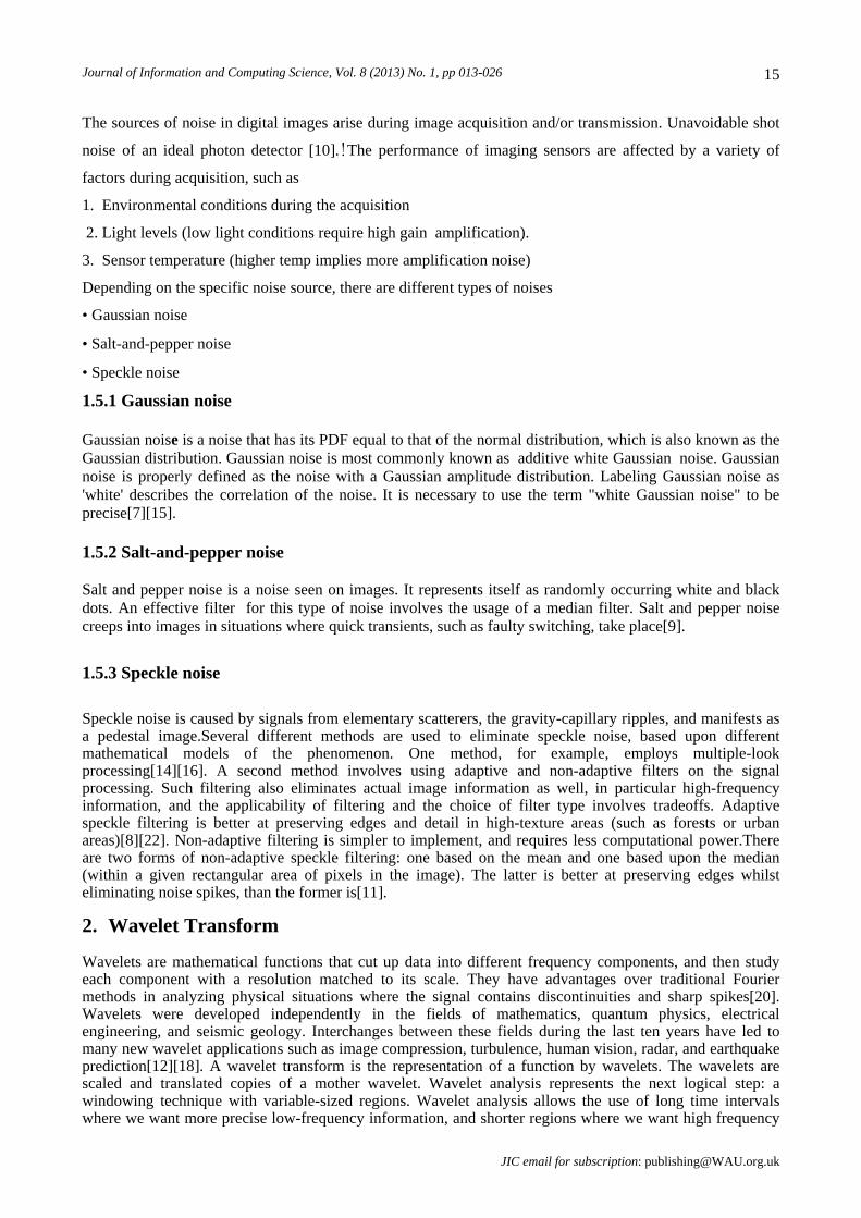
4. Simulation Result The original image is Lena image, adding three types of noise (Gaussian noise, Speckle noise and Salt & Pepper noise) and De-noised image using Average filter, Gaussian filter and Wiener filter, Median filter and Wavelet domain and comparison among them.



17

Fig. 1:Original Lena image taken as reference

Fig 2: Noisy image: Gaussian noise with mean= 0.002 and variance = 0.001

Fig. 3: Noisy image: Speckle noise with variance = 0.005



18

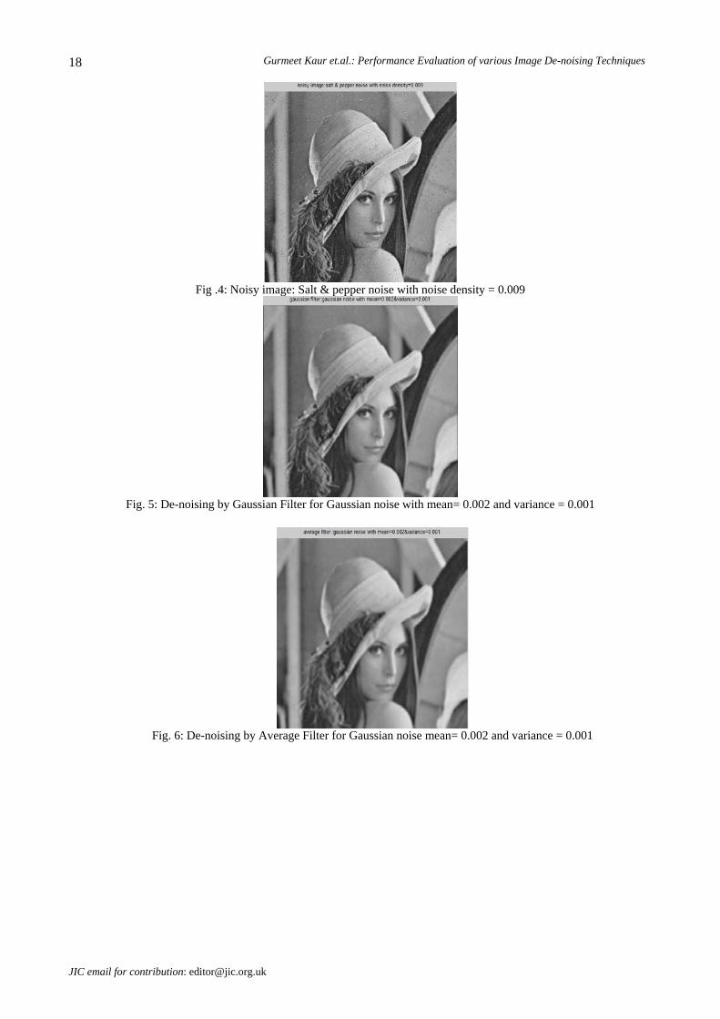
Fig .4: Noisy image: Salt & pepper noise with noise density = 0.009

Fig. 5: De-noising by Gaussian Filter for Gaussian noise with mean= 0.002 and variance = 0.001

Fig. 6: De-noising by Average Filter for Gaussian noise mean= 0.002 and variance = 0.001



19

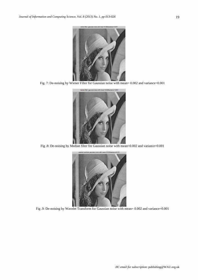
Fig. 7: De-noising by Wiener Filter for Gaussian noise with mean= 0.002 and variance=0.001

Fig .8: De-noising by Median filter for Gaussian noise with mean=0.002 and variance=0.001

Fig .9: De-noising by Wavelet Transform for Gaussian noise with mean= 0.002 and variance=0.001



20

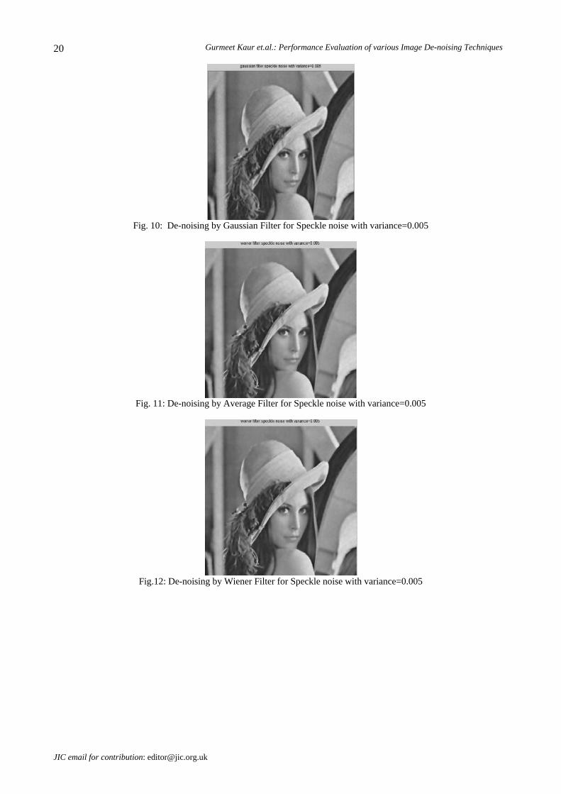
Fig. 10: De-noising by Gaussian Filter for Speckle noise with variance=0.005

Fig. 11: De-noising by Average Filter for Speckle noise with variance=0.005

Fig.12: De-noising by Wiener Filter for Speckle noise with variance=0.005



21

Fig. 13: De-noising by Median filter for Speckle noise with variance=0.005

Fig. 14: De-noising by Wavelet Transform for Speckle noise with variance=0.005

Fig. 15: De-noising by Wiener Filter for Salt & Pepper noise with noise density=0.009



22

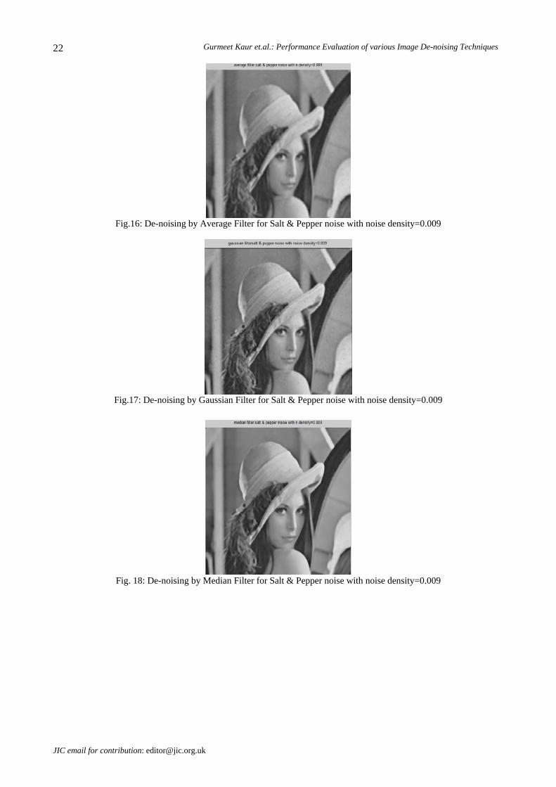
Fig.16: De-noising by Average Filter for Salt & Pepper noise with noise density=0.009

Fig.17: De-noising by Gaussian Filter for Salt & Pepper noise with noise density=0.009

Fig. 18: De-noising by Median Filter for Salt & Pepper noise with noise density=0.009



23

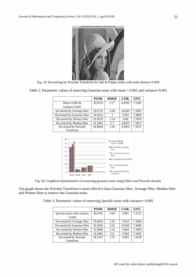
Fig. 19: De-noising by Wavelet Transform for Salt & Pepper noise with noise density=0.009

Table 2: Parametric values of removing Gaussian noise with mean = 0.002 and variance=0.001

PSNR RMSE COR. ENT.

Mean=0.002 & variance=0.001

29.9755 3.17 4.9295 7.5385

De-noised by Average filter 29.6716 3.28 4.9245 7.3693 De-noised by Gaussian filter 30.4553 3 4.935 7.4086 De-noised by Wiener filter 33.3670 2.14 4.68 7.3959 De-noised by Median filter 31.3681 2.7 4.9475 7.3871

De-noised by Wavelet Transform

36.8044 1.44 4.9855 7.4337

Fig. 20: Graphical representation of removing gaussian noise using Filters and Wavelet domain

This graph shows the Wavelet Transform is more effective than Gaussian filter, Average filter, Median filter and Wiener filter to remove the Gaussian noise.

Table 3: Parametric values of removing Speckle noise with variance= 0.005

PSNR RMSE COR. ENT. Speckle noise with variance

=0.005 28.6781 3.68 4.905 7.5312

De-noised by Average filter 29.6620 3.29 4.924 7.3694 De-noised by Gaussian filter 30.3856 3.02 4.9345 7.4088 De-noised by Wiener filter 32.9696 2.25 4.964 7.3983 De-noised by Median filter 31.0491 2.8 4.944 7.3905


38.1953 1.55 4.983 7.4338



24

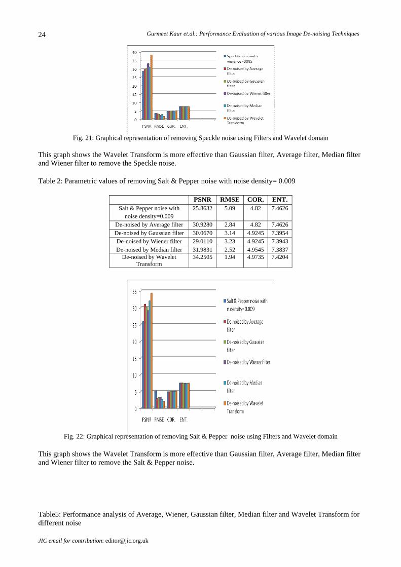
Fig. 21: Graphical representation of removing Speckle noise using Filters and Wavelet domain

This graph shows the Wavelet Transform is more effective than Gaussian filter, Average filter, Median filter and Wiener filter to remove the Speckle noise. Table 2: Parametric values of removing Salt & Pepper noise with noise density= 0.009

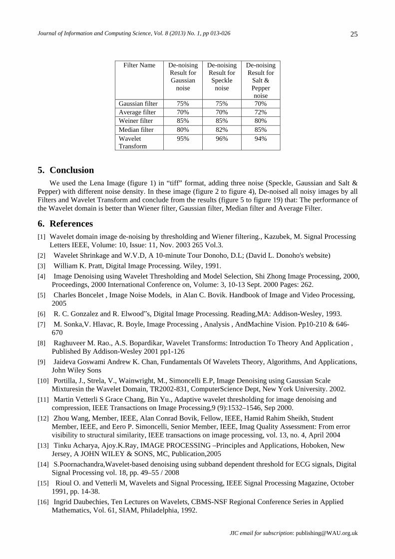
Fig. 22: Graphical representation of removing Salt & Pepper noise using Filters and Wavelet domain

This graph shows the Wavelet Transform is more effective than Gaussian filter, Average filter, Median filter and Wiener filter to remove the Salt & Pepper noise. Table5: Performance analysis of Average, Wiener, Gaussian filter, Median filter and Wavelet Transform for different noise

PSNR RMSE COR. ENT. Salt & Pepper noise with

noise density=0.009 25.8632 5.09 4.82 7.4626

De-noised by Average filter 30.9280 2.84 4.82 7.4626 De-noised by Gaussian filter 30.0670 3.14 4.9245 7.3954 De-noised by Wiener filter 29.0110 3.23 4.9245 7.3943 De-noised by Median filter 31.9831 2.52 4.9545 7.3837


34.2505 1.94 4.9735 7.4204



25

Filter Name De-noising

Result for Gaussian

noise

De-noising Result for Speckle

noise

De-noising Result for

Salt & Pepper noise

Gaussian filter 75% 75% 70% Average filter 70% 70% 72% Weiner filter 85% 85% 80% Median filter 80% 82% 85% Wavelet Transform

95% 96% 94%

5. Conclusion We used the Lena Image (figure 1) in “tiff” format, adding three noise (Speckle, Gaussian and Salt &

Pepper) with different noise density. In these image (figure 2 to figure 4), De-noised all noisy images by all Filters and Wavelet Transform and conclude from the results (figure 5 to figure 19) that: The performance of the Wavelet domain is better than Wiener filter, Gaussian filter, Median filter and Average Filter.

6. References [1] Wavelet domain image de-noising by thresholding and Wiener filtering., Kazubek, M. Signal Processing

Letters IEEE, Volume: 10, Issue: 11, Nov. 2003 265 Vol.3. [2] Wavelet Shrinkage and W.V.D, A 10-minute Tour Donoho, D.L; (David L. Donoho's website) [3] William K. Pratt, Digital Image Processing. Wiley, 1991. [4] Image Denoising using Wavelet Thresholding and Model Selection, Shi Zhong Image Processing, 2000,

Proceedings, 2000 International Conference on, Volume: 3, 10-13 Sept. 2000 Pages: 262. [5] Charles Boncelet , Image Noise Models, in Alan C. Bovik. Handbook of Image and Video Processing,

2005 [6] R. C. Gonzalez and R. Elwood‟s, Digital Image Processing. Reading,MA: Addison-Wesley, 1993. [7] M. Sonka,V. Hlavac, R. Boyle, Image Processing , Analysis , AndMachine Vision. Pp10-210 & 646-

670 [8] Raghuveer M. Rao., A.S. Bopardikar, Wavelet Transforms: Introduction To Theory And Application ,

Published By Addison-Wesley 2001 pp1-126 [9] Jaideva Goswami Andrew K. Chan, Fundamentals Of Wavelets Theory, Algorithms, And Applications,

John Wiley Sons [10] Portilla, J., Strela, V., Wainwright, M., Simoncelli E.P, Image Denoising using Gaussian Scale

Mixturesin the Wavelet Domain, TR2002-831, ComputerScience Dept, New York University. 2002. [11] Martin Vetterli S Grace Chang, Bin Yu., Adaptive wavelet thresholding for image denoising and

compression, IEEE Transactions on Image Processing,9 (9):1532–1546, Sep 2000. [12] Zhou Wang, Member, IEEE, Alan Conrad Bovik, Fellow, IEEE, Hamid Rahim Sheikh, Student

Member, IEEE, and Eero P. Simoncelli, Senior Member, IEEE, Imag Quality Assessment: From error visibility to structural similarity, IEEE transactions on image processing, vol. 13, no. 4, April 2004

[13] Tinku Acharya, Ajoy.K.Ray, IMAGE PROCESSING –Principles and Applications, Hoboken, New Jersey, A JOHN WILEY & SONS, MC, Publication,2005

[14] S.Poornachandra,Wavelet-based denoising using subband dependent threshold for ECG signals, Digital Signal Processing vol. 18, pp. 49–55 / 2008

[15] Rioul O. and Vetterli M, Wavelets and Signal Processing, IEEE Signal Processing Magazine, October 1991, pp. 14-38.

[16] Ingrid Daubechies, Ten Lectures on Wavelets, CBMS-NSF Regional Conference Series in Applied Mathematics, Vol. 61, SIAM, Philadelphia, 1992.



26

[17] Ruskai, M. B. et al., Wavelet and Their Applications, 1992. [18] M. Antonini, M. Barlaud, P. Mathieu, and I. Daubechies, Image coding using wavelet transform, IEEE

Trans. Image Process., vol. 1, no. 2, pp. 205-220, Apr. 1992. [19] J. Woods and J. Kim, Image identification and restoration in the sub band domain, in Proceedings IEEE

Int. Conference on Acoustics, Speech and Signal Processing, San Francisco, CA, vol. III, pp. 297-300, Mar. 1992.

[20] T.L. Ji, M. K. Sundareshan, and H. Roehrig, Adaptive Image Contrast Enhancement Based on Human Visual Properties, IEEE Transactions on Medical Imaging, VOL. 13, NO. 4, December 1994, IEEE

[21] M. R. Banham, Wavelet-Based Image Restoration Techniques, Ph.D. Thesis, Northwestern University, 1994.

performance evaluation of various image de-noising … evaluation of various image de-noising...

Documents