Palestine Polytechnic University

Department of Electronics and Communication Engineering

De-noising of Speech Signal Using Wavelet

Project Submitted in Partial Fulfillmentof the Requirements for the Degree of

Bachelor DegreeIn

Electronics and Communication Engineering

by

Bara' Al frookh

Islam Sharawneh

Mohammad Abu raida

Supervisor :

Dr. Ghandi Manasra

Hebron - Palestine

May 2015

Palestine Polytechnic University

Collage of Engineering

Electrical Engineering Department

Hebron – Palestine

De-noising of Speech Signal Using Wavelet

Project Team

Bara' Al frookh

Islam Sharawneh

Mohammad Abu raida

Submitted to the Collage of Engineering

In partial fulfillment of the requirements for the degree of

Bachelor degree in Electronics and Communication Engineering.

Supervisor Signature

……………………………………….

Testing Committee Signature

……………………………………………………………….…..

Chair of the Department Signature

……………………………………….

June 2015

الاھداء

والحمد الله الذي ھدانا ،ما لم یعلمالإنسانعلم ،الحمد الله الذي علم بالقلموھدوا إلى الطیب "فیھم اللھم اجعلنا ممن قلت ، بھدایتھ ووفقنا بتوفیقھ

. "من القول وھدوا إلى صراط الحمید

راجین منھ یضعھ في میزان نقدم ھذا العمل المتواضع لوجھ االله تعالى .وأن یجعل فیھ البركة والفائدة لكل قارئ لھ،حسناتنا

.أصدقائنا لى أھلنا ونھدي ھذا العمل ا

شكر

نتقدم ومن ھنا، لم یكن ھذا العمل لینجز لولا جھود كثیر من الاشخاصدائرةغاندي مناصرة والى الھیئة التدریسیة في لدكتوربالشكر الى ا

.كنك فلسطینلیتالھندسة الكھربائیة في جامعة بو

i

Abstract

In this project the wavelet de-noising method is used to remove the additivewhite Gaussian noise from noisy speech signals. The idea of wavelet de-noising is toremove the noise by discarding small coefficients of the discrete wavelet transformfor the noisy speech signal. These coefficients can be removed by applying some kindof thresholding function which removes any coefficient below a specific thresholdvalue and keep any coefficient above it. Then, the signal reconstructed by applyinginverse discrete wavelet transform. To evaluate the performance of such algorithm,some kind of performance measure such as signal to noise ratio ( SNR ) can beapplied.

Several methods for speech de-noising using wavelets were tested to evaluatetheir performance. Universal thresholding method is used to threshold the waveletcoefficients. This method uses a fixed threshold for all coefficients, and the thresholdselection depends on the statistical variance measurement. Interval dependentthresholding method is also tested to find its performance, here the signal is dividedinto different interval depends on variance change in it. Then, the threshold value iscalculated for each subinterval depends on the noise variance of each interval. Settingall details coefficients in the first scale to zero by assuming that most of the noisepower in the first level is tested to evaluate the performance such assumption.

Different comparisons are tested such as comparing the performance withdifferent threshold selection rules, comparing the performance with different waveletfamilies, comparing with other filtering technique. The wiener filtering is comparedwith wavelet de-noising method.

ii

Content

Abstract i

Content ii

List of Figures iv

1 Introduction and Motivation 1

1.1 Introduction ……………………………….……………….……………........... 2

1.2 Related works ……………………………….……………….…….…………... 2

1.3 Speech Production ……………………………………………………....…...… 2

1.4 Motivation ……………………………………………………….……..………. 4

1.5 Thesis Outline ………………………………………………….……..………... 4

52 Wavelet Transform and Multiresolution Analysis

2.1 What are wavelets ? …………………………………………………………..... 6

2.2 Haar wavelet ………………………………………………………..………...... 6

2.3 Main idea of wavelet and haar as example …………………………………..… 7

2.4 Wavelet and Fourier Transform : comparison ……………………..…………... 8

2.5 Wavelets and Multiresolution Analysis ………………………..………….....… 8

163 Wavelet De-noising Algorithm

3.1 Wavelet de-noising model ……….………………………………..………..… 17

3.2 Algorithm for speech de-noising ……………………………………………... 21

3.3 Challenges …………………………………………………………………..... 23

3.4 Performance measurement ……………………………………………............ 25

4 Speech enhancement evaluation 26

4.1 Matlab code …………………………………………………………………… 28

4.2 Performance evaluation……………………………………………………….. 38

5 Conclusion and future works 48

5.1 Conclusion ……………………………………………………………………. 49

iii

5.2 Future works…………………………………………………………………... 49

Appendix A 50

Appendix B 59

Appendix C 88

References 90

iv

List of Figures

Fig.1.1 Speech -acoustic product of voluntary and well controlled movement of avocal mechanism of a human ……………………………………………………….. 3

Fig.1.2 The schematic diagram of the human ear ………………………………….... 4

Fig.2.1 Two band filter to extract average and detail of the input signal ………….... 7

Fig.2.2 Average and Difference filters …………………………………………….... 7

Fig.2.3 Haar scaling and wavelet functions …………………………………………. 8

Fig.2.4 One level two channel analysis filter bank ……………………………….... 10

Fig.2.5 One level decomposition of (sinusoidal signal + white noise) …………….. 10

Fig.2.6 One level two channel synthesis filter bank ……………………………….. 11

Fig.2.7 Analysis and Synthesis two channel filter bank ………………………….... 11

Fig.2.8 First channel (low pass channel) in Analysis part …………………………..11

Fig.3.1 Procedure for reconstructing a noisy signal ……………….………………...18

Fig.3.2 Hard and Soft thresholding functions ……………………….……………... 19

Fig.3.3 Block diagram of the de-noising system …………………….…………….. 22

Fig.4.1 Clear and noisy speech signals ……………………………….……………. 30

Fig.4.2 Scaling and wavelet functions, decomposition and reconstruction filters, andFFT of decomposition and reconstruction filtes ……………………….…………… 31

Fig.4.3 Wavelet coefficients for each level ……………………………..………….. 32

Fig.4.5 Reconstructed signals for each level …………………………….…………. 32

Fig.4.5 Energy of coefficients and variance of details at different scales ..………… 33

Fig.4.6 Thresholding functions (soft and hard) …………………………………….. 33

Fig.4.7 Noisy, de-noised and residual signals …………………………………........ 34

Fig.4.8 Comparison between clear signal, noisy signal and de-noised signal ……... 34

Fig.4.9 Correlation between clear speech signal and noisy speech signal, correlationbetween clear speech signal and de-noised speech signal ………………………...... 35

Fig.4.10 Power distribution of clear, noisy and de-noised speech signals …………. 35

v

Fig.4.11 Spectrograms of clear, noisy and de-noised speech signals ………………. 36

Fig.4.12 Comparison between the spectrograms of noisy and de-noised speech signals……………………………………………………………………………………..... 36

Fig.4.13 Absolute coefficients of DWT for clear, noisy and de-noised speechsignals…………………………………………………………………………….…. 37

Fig.4.14 Histograms and cumulative histograms of clear, noisy and de-noised speechsignals ……………………………………………………………………………..... 37

Fig.4.15 Statistical measures of the residual signal ………………………………… 38

Fig.4.16 Output MSE and output SNR after de-noising ………………………….... 38

Fig.4.17a Number of decomposition levels vs. Output SNR using soft thresholdingfunction and universal selection rule ……………………………………………..... 39

Fig.4.17b Input SNR vs. Output SNR using soft thresholding function and universalselection rule ……………………………………………………………………….. 40

Fig.4.18a Number of decomposition levels vs. Output SNR using hard thresholdingfunction and universal selection rule ………………………………………………. 40

Fig.4.18b Input SNR vs. Output SNR using hard thresholding function and universalselection rule ……………………………………………………………………….. 41

Fig.4.19a The threshold value vs. output SNR with different levels of decomposition……………………………………………………………………………………… 42

Fig.4.19b The threshold value vs. output SNR with different input SNRs …….….. 42

Fig.4.20a Input SNR vs. Output SNR for interval-dependent thresholding method. 43

Fig.4.20b Input SNR vs. Output SNR for interval-dependent thresholding method . 44

Fig.4.21a Input SNR vs. Output SNR (Setting all coefficients in the first scale to zero)……………………………………………………………………………................ 44

Fig.4.21b Input SNR vs. Output SNR (Applying soft thresholding on details of firstscale only) ………………………………………………………………………….. 45

Fig.4.22 Input SNR vs. Output SNR with different threshold selection criteria ....... 45

Fig.4.23a Input SNR vs. Output SNR with different type of wavelet families …..... 46

Fig.4.23b The number of decomposition levels vs. output SNR with different waveletfamilies ………………………………………………………………………….…. 46

Fig.4.24 Input SNR vs. Output SNR ( comparison between DWT and WienerFiltering ) …………………………………………………………………………... 47

1

Chapter 1

Introduction and Motivation

1.1 Introduction

1.2 Related works

1.3 Speech Production

1.4 Motivation

1.5 Project Outline

2

Introduction and Motivation

1.1Introduction

Removing of the noise from signals is a key problem in a Digital SignalProcessing field (DSP).

In the mid – 1960s, Dolby noise reduction system was developed for use inanalog magnetic tape recording. Until the beginning of the 1990s, microelectronic andlow cost computer with computation and algorithm design allowed a fast and vastexpansion in the field of digital signal processing researches.

One of the most fundamental problem in the field of speech processing is howthe noise can be removed from the noisy speech signals.

Speech de-noising is the field of studying methods used to recover an originalspeech signal from noisy signals corrupted by different types of noise ( e.g. whitenoise, band-limited white noise, narrow band noise, coloured noise, impulsive noise,transient noise pulses ).These methods can be used in many computers based speechand speaker recognition, coding and mobile communications, hearing aid. Morereduction in noise increases the quality of such application.

The field of speech de-noising includes a lot of researches to improve thespeeches overall quality and increase the speech intelligibility. There are differenttechniques for de-noising the speech signal. Generally speaking the approaches can beclassified into two major categories of single microphone and multi microphonemethods [1].

1.2 Related works

A lot of algorithms proposed to tackle the problem of noise in speech signals,such as Spectral Subtraction [2], Wieiner Filtering [3], Ephraim Malah filtering [4],hidden Markov modeling [5], signal subspace [6].

Gabor [7] introduced a new time – frequency signal analysis. In the field ofmathematic, the papers of mathematicians Mallat [8,9] and Daubechies [10] are a bigcontribution not only in a mathematical side , but also in an engineering applications.These contributions build what so called "multi-rate filter banks basing on wavelettransform".

Mallat and Hwang [11] introduced an algorithm to remove white noises basedon singularity information analysis, Donoho [12] introduced a non linear waveletmethods, Donoho and Johnstone proposed a well known universal waveletthresholding to remove White Gaussian Noise (WGN) [Donoho12,13] ,[Donoho andjohnstone 14], Johnstone and Silverman [15] proposed level dependant thresholdingenhancement method.

1.3 Speech Production

In order to apply DSP techniques to speech processing problems, it isimportant to understand the fundamentals of the speech production process, [16].

3

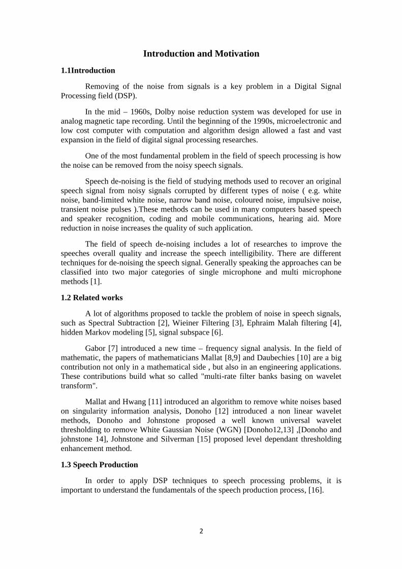
Speech is the acoustic product of voluntary and well-controlled movement of avocal mechanism of a human (see fig.1.1). During the generation of speech, air isinhaled into the human lungs by expanding the rib cage and drawing it in via the nasalcavity, velum and trachea it is then expelled back into the air by contracting the ribcage and increasing the lung pressure. During the expulsion of air, the air travels fromthe lungs and passes through vocal cords which are the two symmetric pieces ofligaments and muscles located in the larynx on the trachea. Speech is produced by thevibration of the vocal cords. Before the expulsion of air, the larynx is initially closed.When the pressure produced by the expelled air is sufficient, the vocal cords arepushed apart, allowing air to pass through. The vocal cords close upon the decrease inair flow. This relaxation cycle is repeated with generation frequencies in the range of80Hz – 300Hz. The generation of this frequency depends on the speaker‘s age, sex,stress and emotions. This succession of the glottis openings and closure generatesquasi-periodic pulses of air after the vocal cords. The speech signal is a time varyingsignal whose signal characteristics represent the different speech sounds produced.There are three ways of labelling events in speech. First is the silence state in whichno speech is produced. Second state is the unvoiced state in which the vocal cords arenot vibrating, thus the output speech waveform is a periodic and random in nature.The last state is the voiced state in which the vocal cords are vibrating periodicallywhen air is expelled from the lungs. This results in the output speech being quasi-periodic- shows a speech waveform with unvoiced and voiced state. Speech isproduced as a sequence of sounds. The type of sound produced depends on shape ofthe vocal tract. The vocal tract starts from the opening of the vocal cords to the end ofthe lips. Its cross sectional area depends on the position of the tongue, lips, jaw andvelum. Therefore the tongue, lips, jaw and velum play an important part in theproduction of speech.[17]

Fig.1.1:Speech -acoustic product of voluntary and well controlled movement of avocal mechanism of a human

4

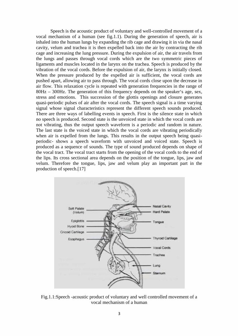
Audible sounds are transmitted to the human ears through the vibration of theparticles in the air. Human ears consist of three parts, the outer ear, the middle ear andthe inner ear. The function of the outer ear is to direct speech pressure variationstoward the eardrum where the middle ear converts the pressure variations intomechanical motion. The mechanical motion is then transmitted to the inner ear, whichtransforms these motion into electrical potentials that passes through the auditorynerve, cortex and then to the brain . Figure (fig.1.2) below shows the schematicdiagram of the human ear.[17]

Fig.1.2: The schematic diagram of the human ear

1.4 Motivation

Speech is a native way for human communication and it considered one of themost important signals in multimedia system. Noise is presented in a speech signaldue to communication channel. Removing the noise to improve the quality of speechis needed. One of the most important kind of noise is the white noise which is randomand its power spectral density is constant. Specifically, Gaussian noise is normallydistributed and generated by almost all natural phenomena.

Speech signal is a non-stationary signal. The wavelet transform is consideredas appropriate choice to analyze local variations in signals. The multi-resolutionproperties of wavelet analysis reflect the frequency resolution of the human earsystem. Most of data that represent the speech signal are not totally random, there is acertain correlation structure. The harmonic signals content is closely correlated, andthis means that large coefficients represent the speech signal and the small valuesrepresent the uncorrelated noise. Thus, the noise can be removed by discarding thesmall coefficients.

1.5 Project Outline

The structure of this project is as follows, in chapter 2 some of backgroundabout wavelets, filter banks and multi-resolution theory. Wavelet de-noising modeland algorithm design are presented in chapter 3. The speech quality evaluation andperformance of algorithm are presented in chapter 4,conclusion is shown in chapter 5.

5

Chapter 2

Wavelet transform and multiresolution analysis

2.1 What are wavelets ?

2.2 Haar wavelet

2.3 Main idea of wavelet and haar as example

2.4 Wavelet and Fourier Transform: comparison

2.5 Wavelets and Multiresolution Analysis

6

Wavelet transform and multiresolution analysis

In this chapter, we will briefly introduce the background behind the wavelet transformand multiresoltion analysis. This introduction will be as short as possible. There areseveral papers and articles talking about wavelets. For more details one can refer to[18 - 27].

2.1 What are wavelets ?

Wavelets are oscillatory waveforms of finite duration and zero average value.These waveforms must be localized. There are many mathematical conditions must besatisfied to ensure that an oscillatory function is admissible as a wavelet basisfunction. There are many kinds of wavelets whose characteristics vary according tomany criteria. One can choose between smooth wavelets, compactly supportedwavelets, orthogonal wavelets, symmetrical wavelets, wavelets with simplemathematical expressions, wavelets with simple associated fitters, etc. The simplestand the most important wavelet is the Haar wavelet, and we discuss it as anintroductory example in the next section.

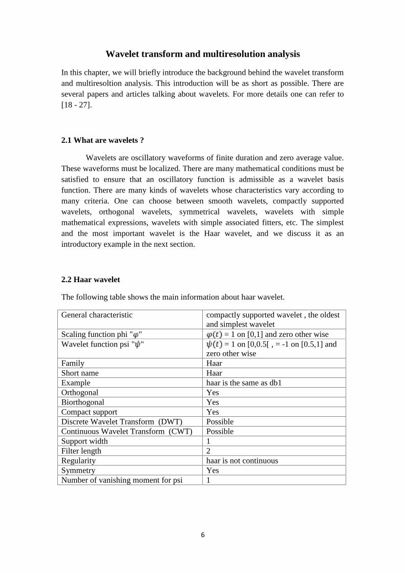
2.2 Haar wavelet

The following table shows the main information about haar wavelet.

General characteristic compactly supported wavelet , the oldestand simplest wavelet

Scaling function phi " " = 1 on [0,1] and zero other wiseWavelet function psi " " = 1 on [0,0.5[ , = -1 on [0.5,1] and

zero other wiseFamily HaarShort name HaarExample haar is the same as db1Orthogonal YesBiorthogonal YesCompact support YesDiscrete Wavelet Transform (DWT) PossibleContinuous Wavelet Transform (CWT) PossibleSupport width 1Filter length 2Regularity haar is not continuousSymmetry YesNumber of vanishing moment for psi 1

7

2.3 Main idea of wavelet and haar as example

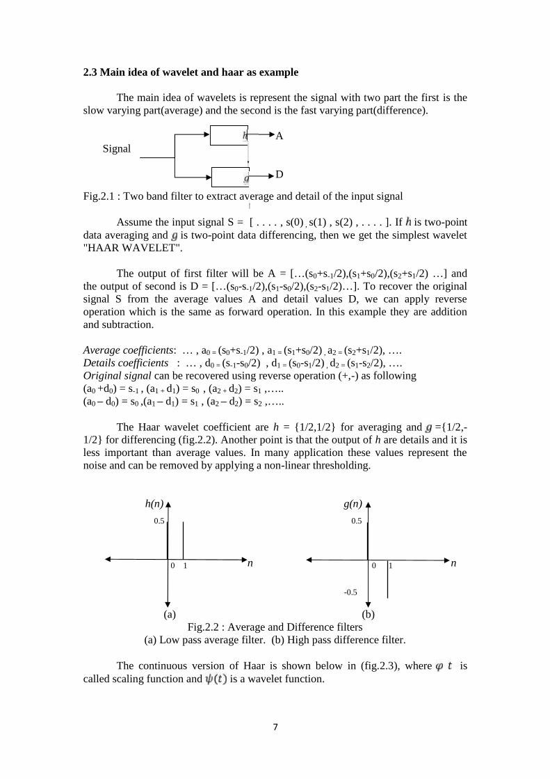
The main idea of wavelets is represent the signal with two part the first is theslow varying part(average) and the second is the fast varying part(difference).

ASignal

D

Fig.2.1 : Two band filter to extract average and detail of the input signal

Assume the input signal S = [ . . . . , s(0) , s(1) , s(2) , . . . . ]. If is two-pointdata averaging and is two-point data differencing, then we get the simplest wavelet"HAAR WAVELET".

The output of first filter will be A = […(s0+s-1/2),(s1+s0/2),(s2+s1/2) …] andthe output of second is D = […(s0-s-1/2),(s1-s0/2),(s2-s1/2)…]. To recover the originalsignal S from the average values A and detail values D, we can apply reverseoperation which is the same as forward operation. In this example they are additionand subtraction.

Average coefficients: … , a0 = (s0+s-1/2) , a1 = (s1+s0/2) , a2 = (s2+s1/2), ….Details coefficients : … , d0 = (s-1-s0/2) , d1 = (s0-s1/2) , d2 = (s1-s2/2), ….Original signal can be recovered using reverse operation (+,-) as following(a0 +d0) = s-1 , (a1 + d1) = s0 , (a2 + d2) = s1 ,…..(a0 – d0) = s0 ,(a1 – d1) = s1 , (a2 – d2) = s2 ,…..

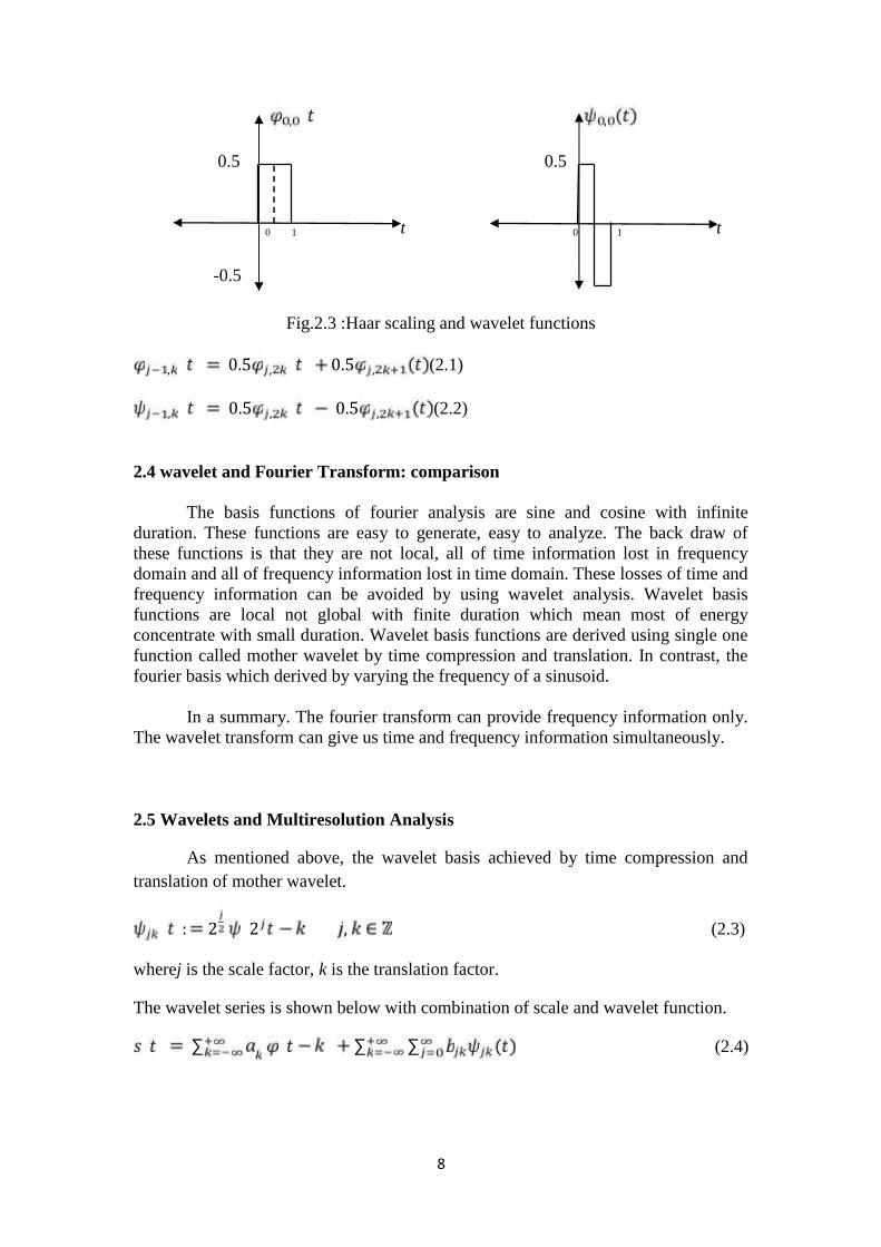
The Haar wavelet coefficient are h = {1/2,1/2} for averaging and ={1/2,-1/2} for differencing (fig.2.2). Another point is that the output of h are details and it isless important than average values. In many application these values represent thenoise and can be removed by applying a non-linear thresholding.

h(n) g(n)

0.5 0.5

0 1 n 0 1 n

-0.5

(a) (b)Fig.2.2 : Average and Difference filters

(a) Low pass average filter. (b) High pass difference filter.

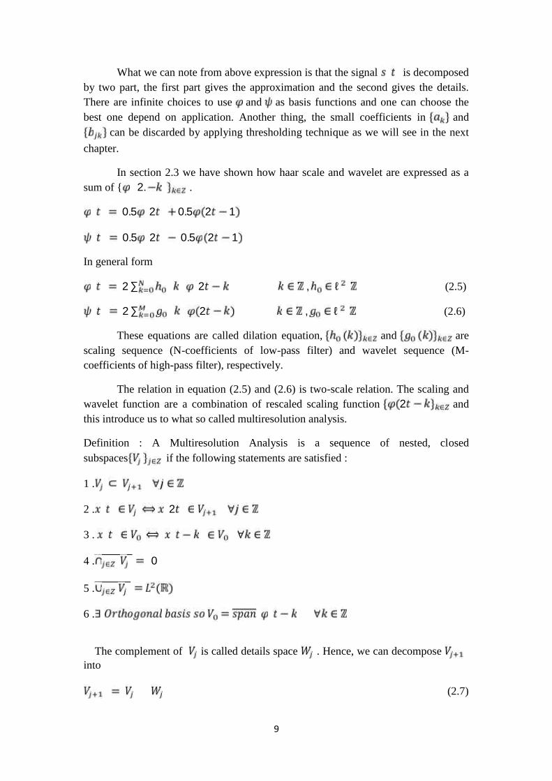
The continuous version of Haar is shown below in (fig.2.3), where iscalled scaling function and is a wavelet function.

8

, ,0.5 0.5

0 1 t 0 1 t

-0.5

Fig.2.3 :Haar scaling and wavelet functions

, 0.5 , 0.5 , (2.1)

, 0.5 , 0.5 , (2.2)

2.4 wavelet and Fourier Transform: comparison

The basis functions of fourier analysis are sine and cosine with infiniteduration. These functions are easy to generate, easy to analyze. The back draw ofthese functions is that they are not local, all of time information lost in frequencydomain and all of frequency information lost in time domain. These losses of time andfrequency information can be avoided by using wavelet analysis. Wavelet basisfunctions are local not global with finite duration which mean most of energyconcentrate with small duration. Wavelet basis functions are derived using single onefunction called mother wavelet by time compression and translation. In contrast, thefourier basis which derived by varying the frequency of a sinusoid.

In a summary. The fourier transform can provide frequency information only.The wavelet transform can give us time and frequency information simultaneously.

2.5 Wavelets and Multiresolution Analysis

As mentioned above, the wavelet basis achieved by time compression andtranslation of mother wavelet.: 2 2 , (2.3)

wherej is the scale factor, k is the translation factor.

The wavelet series is shown below with combination of scale and wavelet function.∑ ∑ ∑ (2.4)

9

What we can note from above expression is that the signal is decomposedby two part, the first part gives the approximation and the second gives the details.There are infinite choices to use and as basis functions and one can choose thebest one depend on application. Another thing, the small coefficients in and

can be discarded by applying thresholding technique as we will see in the next

chapter.

In section 2.3 we have shown how haar scale and wavelet are expressed as asum of { 2. .0.5 2 0.5 2 10.5 2 0.5 2 1In general form2 ∑ 2 , ℓ (2.5)2 ∑ 2 , ℓ (2.6)

These equations are called dilation equation, and arescaling sequence (N-coefficients of low-pass filter) and wavelet sequence (M-coefficients of high-pass filter), respectively.

The relation in equation (2.5) and (2.6) is two-scale relation. The scaling andwavelet function are a combination of rescaled scaling function 2 andthis introduce us to what so called multiresolution analysis.

Definition : A Multiresolution Analysis is a sequence of nested, closedsubspaces if the following statements are satisfied :

1 .

2 . 23 .

4 . 05 .

6 .

The complement of is called details space . Hence, we can decomposeinto

(2.7)

10

As an example, from equation (2.5) we see that , and fromequation (2.6) we see that , and this imply that

(2.8)

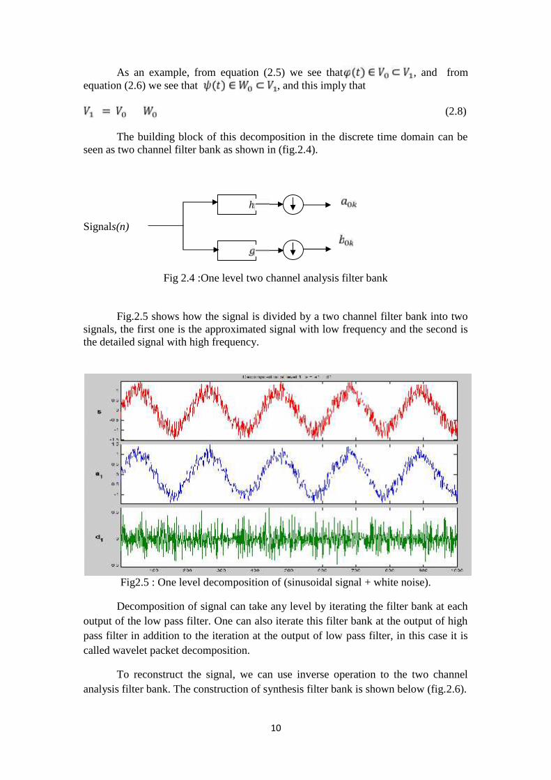
The building block of this decomposition in the discrete time domain can beseen as two channel filter bank as shown in (fig.2.4).

Signals(n)

Fig 2.4 :One level two channel analysis filter bank

Fig.2.5 shows how the signal is divided by a two channel filter bank into twosignals, the first one is the approximated signal with low frequency and the second isthe detailed signal with high frequency.

Fig2.5 : One level decomposition of (sinusoidal signal + white noise).

Decomposition of signal can take any level by iterating the filter bank at eachoutput of the low pass filter. One can also iterate this filter bank at the output of highpass filter in addition to the iteration at the output of low pass filter, in this case it iscalled wavelet packet decomposition.

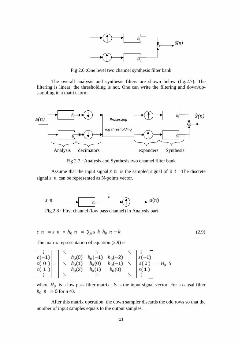
To reconstruct the signal, we can use inverse operation to the two channelanalysis filter bank. The construction of synthesis filter bank is shown below (fig.2.6).

11

(n)

Fig 2.6 :One level two channel synthesis filter bank

The overall analysis and synthesis filters are shown below (fig.2.7). Thefiltering is linear, the thresholding is not. One can write the filtering and down/up-sampling in a matrix form.

Analysis decimators expanders Synthesis

Fig 2.7 : Analysis and Synthesis two channel filter bank

Assume that the input signal is the sampled signal of . The discretesignal can be represented as N-points vector.

Fig.2.8 : First channel (low pass channel) in Analysis part

∑ (2.9)

The matrix representation of equation (2.9) is

101 =0 1 21 0 12 1 0 101 =

where is a low pass filter matrix , S is the input signal vector. For a causal filter0 for n<0.

After this matrix operation, the down sampler discards the odd rows so that thenumber of input samples equals to the output samples.

Processing

e.g thresholding

(n) (n)

16

Chapter 3

Wavelet de-noising algorithm

3.1 Wavelet de-noising model

3.2 Algorithm for speech de-noising

3.3 Challenges

3.4 Performance measurement

17

Wavelet de-noising algorithm

3.1 Wavelet de-noising model

Wavelet de-noising is a non-parametric method which does not needparameter estimation of the speech enhancement model. Estimating the signalcorrupted by Gaussian noise is considered as an important problem in many studies,and it will be our interest in this project. We will restrict our study only to AdditiveWhite Gaussian noise.

Let us consider a speech signal , and an independently and identicallyadditive white gaussian noise ~ 0, , the noisy signal can be written as follows

, ,….., (3.1)

The goal of wavelet de-noising is to find an approximation to the signal ,that minimize the mean squared error ∑ (3.2)

Where and Applying the wavelet transform matrix , the equation (3.1) becomes as follows

(3.3)

, , , (3.4)

where . , are the wavelet coefficients.

Because of using orthogonal transform to express in an orthogonalwavelet basis, the wavelet coefficients of the i.i.d Gaussian noise are also i.i.dGaussian. This kind of transformation preserved the statistical independence of thenoise and it is called a unitary transform.

By choosing a good matched wavelet for signal representation, the noisepower will tend to concentrate in a small coefficients while the most of signal powerwill be in large coefficients. This idea of a sparse representation due to the wavelettransform allows us to remove the noise from the signal by discarding the smallcoefficients which represent the noise. To do that we need to apply a waveletthresholding function . on a wavelet coefficients.

, , , (3.5)

, , , (3.6)

where . , are the wavelet coefficient after thresholding.

18

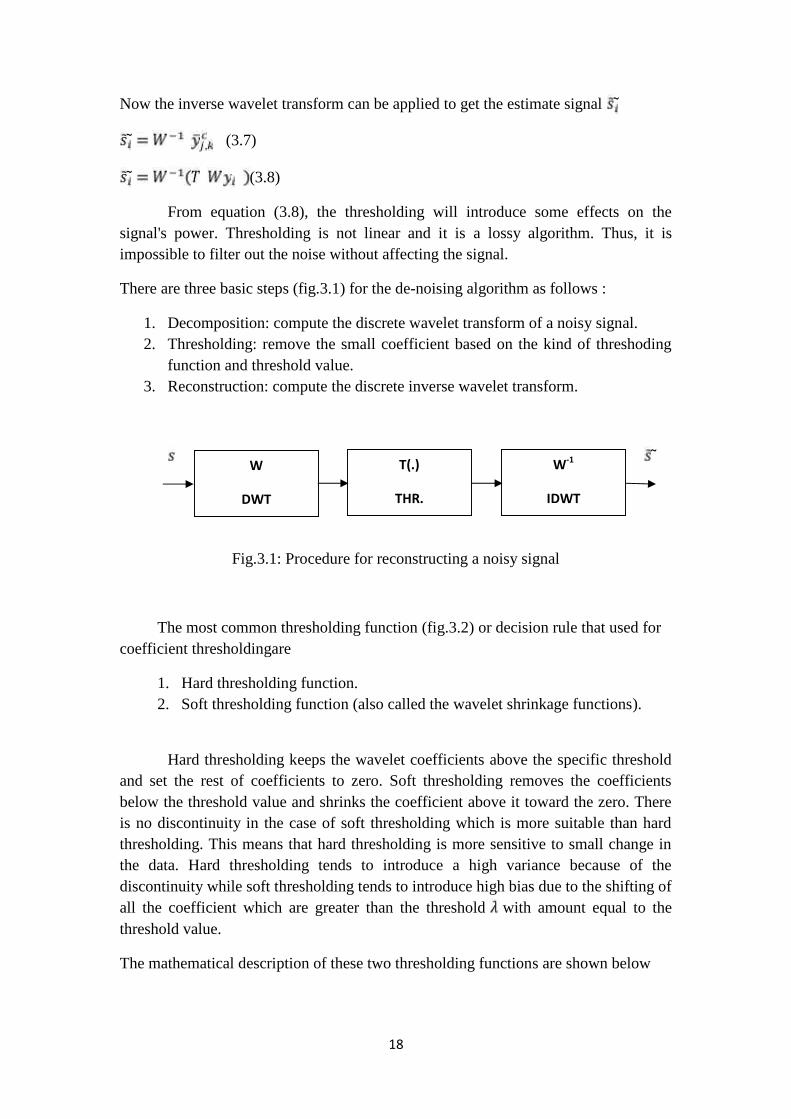
Now the inverse wavelet transform can be applied to get the estimate signal , (3.7) (3.8)

From equation (3.8), the thresholding will introduce some effects on thesignal's power. Thresholding is not linear and it is a lossy algorithm. Thus, it isimpossible to filter out the noise without affecting the signal.

There are three basic steps (fig.3.1) for the de-noising algorithm as follows :

1. Decomposition: compute the discrete wavelet transform of a noisy signal.2. Thresholding: remove the small coefficient based on the kind of threshoding

function and threshold value.3. Reconstruction: compute the discrete inverse wavelet transform.

Fig.3.1: Procedure for reconstructing a noisy signal

The most common thresholding function (fig.3.2) or decision rule that used forcoefficient thresholdingare

1. Hard thresholding function.2. Soft thresholding function (also called the wavelet shrinkage functions).

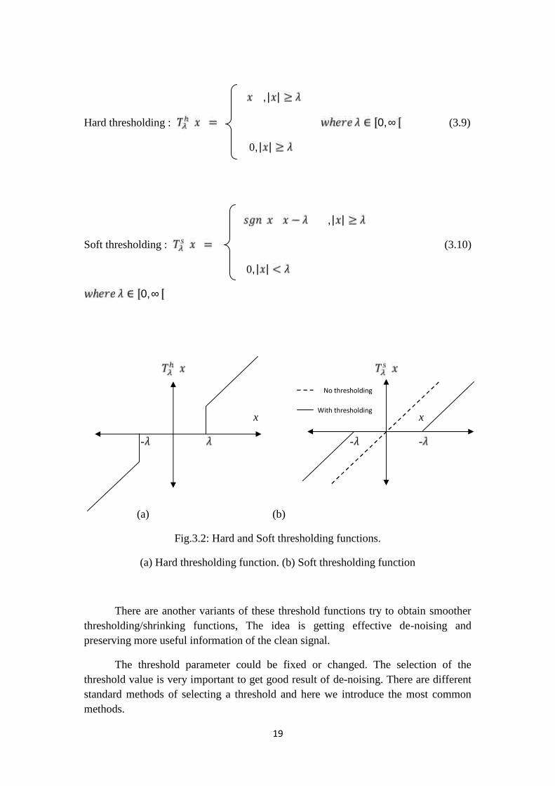
Hard thresholding keeps the wavelet coefficients above the specific thresholdand set the rest of coefficients to zero. Soft thresholding removes the coefficientsbelow the threshold value and shrinks the coefficient above it toward the zero. Thereis no discontinuity in the case of soft thresholding which is more suitable than hardthresholding. This means that hard thresholding is more sensitive to small change inthe data. Hard thresholding tends to introduce a high variance because of thediscontinuity while soft thresholding tends to introduce high bias due to the shifting ofall the coefficient which are greater than the threshold with amount equal to thethreshold value.

The mathematical description of these two thresholding functions are shown below

W

DWT

T(.)

THR.

W-1

IDWT

19

, | |Hard thresholding : 0, ∞ (3.9)

0, | |, | |

Soft thresholding : (3.10)

0, | |0, ∞

x x

- - -

(a) (b)

Fig.3.2: Hard and Soft thresholding functions.

(a) Hard thresholding function. (b) Soft thresholding function

There are another variants of these threshold functions try to obtain smootherthresholding/shrinking functions, The idea is getting effective de-noising andpreserving more useful information of the clean signal.

The threshold parameter could be fixed or changed. The selection of thethreshold value is very important to get good result of de-noising. There are differentstandard methods of selecting a threshold and here we introduce the most commonmethods.

No thresholding

With thresholding

20

1. Universal method :

It is a fixed threshold de-noising method and the proper selection of the threshold fora discrete wavelet transform (DWT) is determined as follow2 (3.11)

where N is the length (number of samples) in the noisy signal and is an estimate ofthe standard deviation of zero mean additive white gaussian noise calculated by thefollowing median absolute deviation formula

,. (3.12)

where , is the details wavelet coefficient sequence of the noisy signal on first level.

For a wavelet packet transform (WPT), the threshold can be calculated by2 (3.13)

where is the noisy signal length and is the standard deviation.

The universal threshold method uses global thresholds. This means, thecomputed threshold is used for all coefficients. This method of threshold selectiondepends on the statistical variance measurement of the noise and noisy signal lengthonly.

2 .Minimaxmethod :

In this method, the threshold will be selected by minimizing the error betweenthe wavelet coefficient of noisy signal and original signal. The noisy signal can beseen as unknown regression function, this kind of estimator can minimize themaximum mean square error for a given unknown regression function.

The threshold value can be calculated by

(3.14)

where is calculated by a minimax rule such that the maximum error across the datais minimized.

The threshold selection in this method is independent of any signalinformation. Thus, it is good primarily choice for completely unknown signalinformation.

3 . SURE method :

SURE (Stein's unbiased risk estimator) is an adaptive thresholdingmethod thatuses a threshold value at each resolution level j of the wavelet coefficients. In the

level dependent universal threshold, the threshold at each scale j is selected as

21

2 (3.15)

where is the samples number in the scale j and is an estimate of the standard

deviation in the scale j.

This method is a good choice for non-stationary noise, in this case the varianceof the noise wavelet coefficients will differ for different scales in the waveletdecomposition.

Adaptive thresholding can be used to enhance the performance of de-noisingalgorithm, The threshold can be selected based on the data information in any genericdomain. One choice of generic domain is the energy of the data. The threshold valuedepends not only on N but also on the energy of the data frame as follows

(3.16)

where is the energy of the data frame in a signal.

Since the speech and the noise are uncorrelatedand , from equation (3.1) and(3.4), we have the following relations

(3.17)

(3.18)

where E is the signal energy in the frame

Equation (3.17) and (3.18) show that the energy of the noisy speech signalframe in the wavelet domain is equal to the energy of the noisy signal in a timedomain. The energy transformation between time and wavelet domains is preserved.

In this project, we only concentrate our study about a single channel (singlemicrophone) speech de-noising system which does not use multi-channel for noisereduction.

3.2 Algorithm for speech de-noising

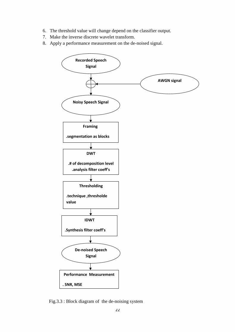
The main steps of the de-noising procedure are shown below. Fig.3.3 showsthe flow chart of algorithm for speech de-noising.

Summary of the algorithm :

1. Add a random additive white Gaussian noise to the clean signal.2. Segment the noisy signal into frames.3. Make the discrete wavelet transform for every input frame.4. Calculate the energy of wavelet coefficient and zero crossing rate.5. Based on the previous point, the feature of the frame is extracted to classify

every noisy speech frame into one of three classes (voiced/unvoiced/silence).

22

6. The threshold value will change depend on the classifier output.7. Make the inverse discrete wavelet transform.8. Apply a performance measurement on the de-noised signal.

Fig.3.3 : Block diagram of the de-noising system

Performance Measurement

. SNR, MSE

Thresholding

.technique ,thresholdevalue

IDWT

.Synthesis filter coeff's

Recorded SpeechSignal

DWT

.# of decomposition level.analysis filter coeff's

Noisy Speech Signal

De-noised SpeechSignal

Framing

.segmentation as blocks

AWGN signal

23

3.3 Challenges

Some challenges in applying the above algorithm :

1. Segmentation.2. Voiced / unvoiced / silence.3. Filter coefficients of analysis and synthesis.4. Number of decomposition levels.5. Thresholding type.6. Threshold value is very important parameter.7. Level of noise.

Now, let's proceed to investigate these challenges in more depth.

The first challenge is to segment the speech signal with proper frame duration,the frame with N samples can be conceived as N dimensional vector space, and whenanalyzing this vector of samples some features contained in the frame could be lost ifwe do not choose the proper framing mythology. The solution of this problem can besolved by introducing overlap frames. By choosing a proper widow for segmentationwith some percent of overlapping we can minimize the losses of features in the frame.

Each frame will typically contain 100 sample if we assume the samplingfrequency equal to 8 KHz. This imply that the frame duration will be 12.5 ms. Weneed to choose the number of sample in each frame as a power of 2 to avoid usingsignal extension(e.g.128samples). .

The second challenge is that when applying the thresholding on the speechsignal, the possibility of speech degradation is exist since some of frame is unvoicedwhich mean that most of energy of the frame is concentrated in the high frequencybands and eliminating of them will make a degradation in the quality of the de-noisedsignal.The solution of this problem is the most hardest part in this algorithm. Howeverby choosing a proper decision rule for classification process we can avoid the speechdegradation. Here we introduce two features and its equations

. Short – term average energy :

∑ | | (3.19)

where N is the frame length and l is the data index.

. Zero crossing rate: calculate the number of sign changes of successivesamples in the frame.

∑ 1 (3.20)

24

where is the signum function.

These features are typically estimated for frames of speech with 10-20 ms duration.

The choice of widow type determines the nature of short-term average energyrepresentation. If size of the widow is very long, then it is equivalent to a verynarrowband low pass filter, that means the short term energy will reflect the amplitudevariation in a speech signal.In contrast, if the window size is very short, the short-term

energy will not provide a sufficient energy averaging.

Zero crossing rate reflects the frequency content in the frame. It is important toremove any offset in a signal to ensure a correct calculation in the case of zerocrossing rate.

We can use short term energy and zero crossing rate to change the threshold valuebased on Voiced/Unvoiced/Silence classification.

. High energy and low zero crossing rate imply that the frame is voiced.

- Most of the power for the voiced frame is contained in the approximation partof wavelet decomposition.

. Low energy and high zero crossing rate imply that the frame is unvoiced.

- Most of the power for the unvoiced frame is contained in the details part ofwavelet decomposition.

. Relatively equal power distribution imply that the frame is silence.

The third challenge is about the wavelet filter design. Choosing an appropriatefilter coefficient is considered a critical part in all of this process of de-noising. Thereare several criteria that could be used to select the best wavelet filter. In this projectwe tended to use the most simple and the most important filter bank which is the Haarfilter. This filter is considered as a good choice since it has a different property suchas symmetry, orthogonality, biorthogonality, compactness and sparsity. We willinvestigate many other db wavelets with higher vanishing moments.

The fourth challenge is selecting the number of levels for waveletdecomposition. Generally speaking, the number of needed level for decompositionwill increase as the power noise increases, however, increasing the levels ofdecomposition increase the computational complexity in the wavelet de-noisingalgorithm. Practically, increasing the number of the level more than five will notintroduce a very significant change in the output signal to noise ratio. The selection ofnumber of levels will depend on the kind of the signal or on some criteria as entropy.

The fifth challenge is choosing an appropriate threshold function, in thisproject we intend to use soft thresholding function since it is more stable than hardthresholding.

25

The sixth challenge is about how we can choose the threshold value. Asdiscussed in the previous section the threshold should be adapted to avoid the speechdegradation, the choice of threshold will be chosen such that the small coefficients arebest threshold with high threshold values, whereas the small coefficients needed to bethreshold with small threshold values. .

The seventh challenge is about the level power of the additive noise.Practically, if the SNRs of the noisy signal is very low, such this method will failsince the noisy coefficient will becomes significantly large so that it is difficult todistinguish between the clean and noisy coefficient. In this project the signal to noiseratio level will be about 0 dB to 20 dB.

Actually, speech is a complex noise process and these are not the onlychallenges nor the only typical solution. There are a lot of optimization and adaptationprocess to get more optimum de-noising algorithm that could be used with a diverseconditions.

For performance measurement, objective and subjective quality can be used toprovide a measure how much improvement occurred before the processing. The goalis to increase the output signal to noise ratio (SNR) in each frame such that theaverage SNR isincreased.

Objectively, there are two common measure as follows

. Signal to noise ratio SNR :

, ∑∑ (3.23)

where , is the segmental output signal to noise ratio of the frame ,

is the input frame of the clean speech signal and is the output enhancedframe of the speech signal.

. Mean Square Error MSE :∑ 3.22frame.where is a mean squared error in the

26

Chapter 4Speech enhancement evaluation

4.1 Matlab code

4.2 Performance evaluation

27

Speech enhancement evaluation

In this chapter we are going to construct a matlab code for the wavelet de-noisingalgorithm and tackle the different challenges which discussed in previous chapter. After that, thediscussion about the results is introduced in the context of the performance evaluation.

As mentioned before, the main three steps in the de-noising algorithm using waveletthresholding are decoposition, thresholding and reconstruction. Every step in this algorithm isimplemented using matlab programming language. The Wavelet Toolbox in Matlab containsvarious functions that can be called to build the de-noising algorithm. This kind of programmingis called a procedural programming which is a programming paradigm, derived fromstructuredprogramming. The abstraction nature of the function in Matlab is an input-output relation asshown below

[ output arguments ] = functionName( input arguments )

The above statement uses to call the functions built in Matlab. To get an informationabout how to use a given function, Matlab provides an help documentation about using thefunctions e.g. ( doc functionName , help functionName). To get the details about the code ofany function, the command ( edit functionName ) can be used.

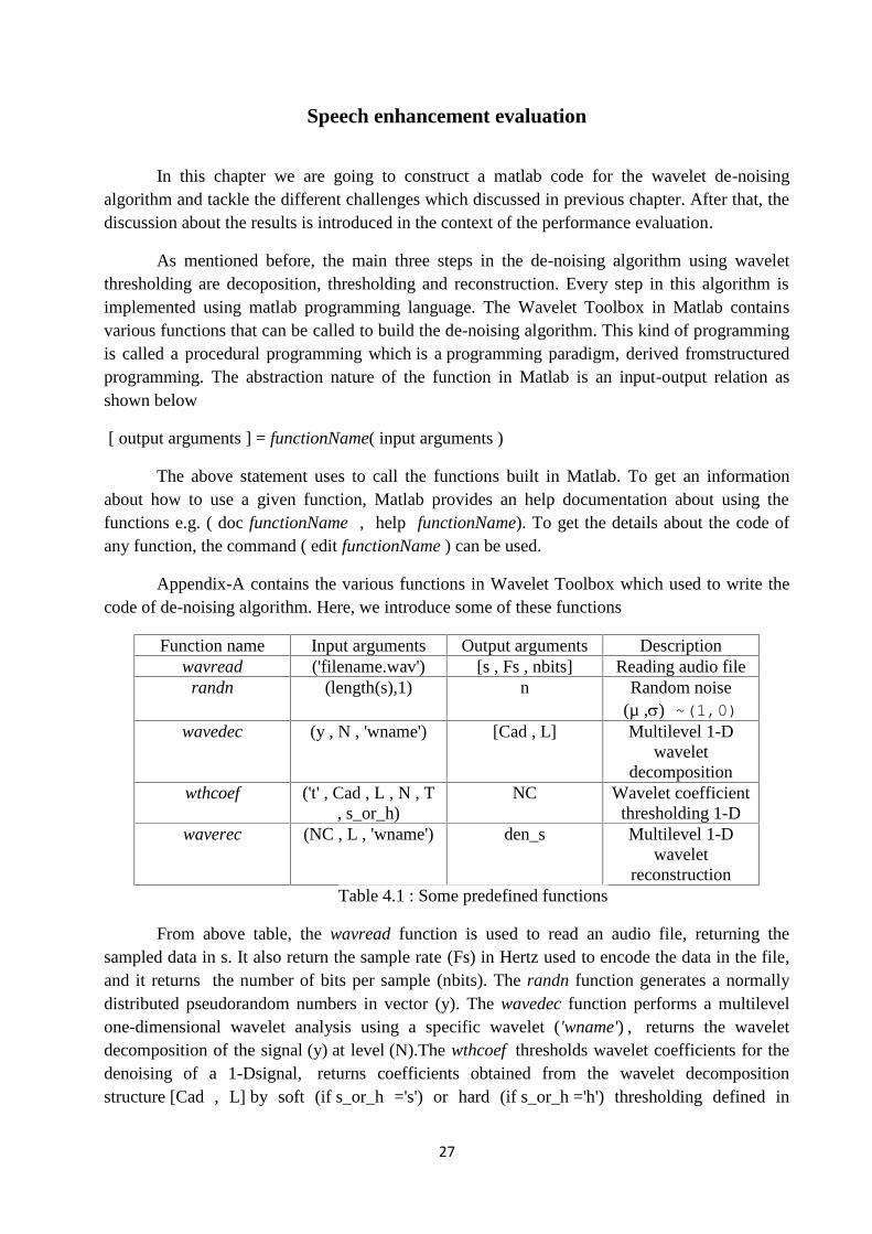
Appendix-A contains the various functions in Wavelet Toolbox which used to write thecode of de-noising algorithm. Here, we introduce some of these functions

Function name Input arguments Output arguments Descriptionwavread ('filename.wav') [s , Fs , nbits] Reading audio file

randn (length(s),1) n Random noise(µ ,) ~(1,0)

wavedec (y , N , 'wname') [Cad , L] Multilevel 1-Dwavelet

decompositionwthcoef ('t' , Cad , L , N , T

, s_or_h)NC Wavelet coefficient

thresholding 1-Dwaverec (NC , L , 'wname') den_s Multilevel 1-D

waveletreconstruction

Table 4.1 : Some predefined functions

From above table, the wavread function is used to read an audio file, returning thesampled data in s. It also return the sample rate (Fs) in Hertz used to encode the data in the file,and it returns the number of bits per sample (nbits). The randn function generates a normallydistributed pseudorandom numbers in vector (y). The wavedec function performs a multilevelone-dimensional wavelet analysis using a specific wavelet ('wname') , returns the waveletdecomposition of the signal (y) at level (N).The wthcoef thresholds wavelet coefficients for thedenoising of a 1-Dsignal, returns coefficients obtained from the wavelet decompositionstructure [Cad , L] by soft (if s_or_h ='s') or hard (if s_or_h ='h') thresholding defined in

28

vectors (N) and (T). Vector (N) contains the detail levels to be thresholded and vector (T) is thecorresponding thresholds. (N) and (T) must be of the same length. The waverec functionperforms a multilevel one-dimensional wavelet reconstruction using a specific wavelet ('wname'), reconstructs the signal (den_s) based on the multilevel wavelet decomposition structure [NC ,L]. For more information about many different functions for wavelet analysis, Reference [ ]provide a lot of details about these functions.

4.1 Matlabcode

Appendix-B shows the Matlab code for de-noising the speech signals. It includes manyoptions that can be used to provide illustrative steps of wavelet de-noising method. The firstsubsection of this section introduces the different options of this Matlabprogram, the nextsubsection shows an illustrative example of using the program.

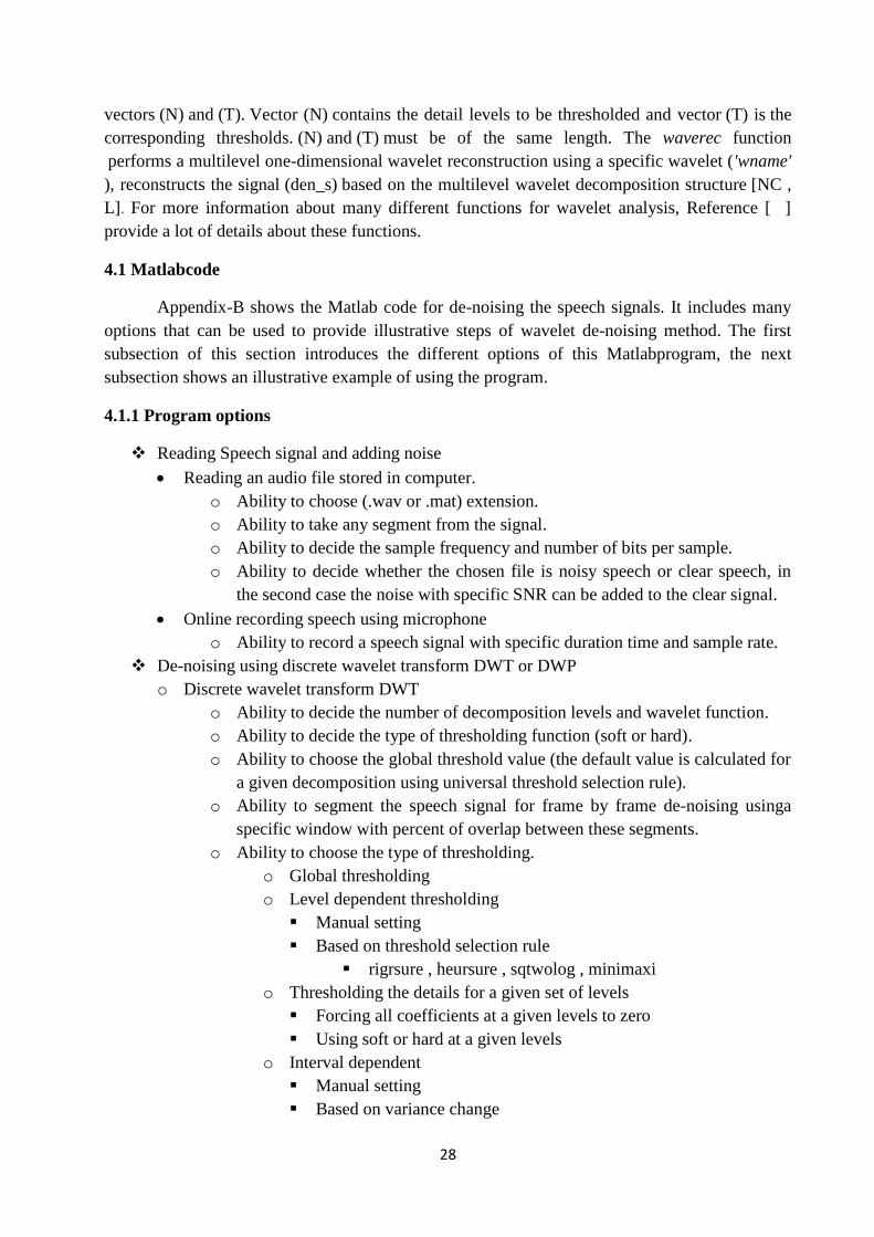
4.1.1 Program options

Reading Speech signal and adding noise Reading an audio file stored in computer.

o Ability to choose (.wav or .mat) extension.o Ability to take any segment from the signal.o Ability to decide the sample frequency and number of bits per sample.o Ability to decide whether the chosen file is noisy speech or clear speech, in

the second case the noise with specific SNR can be added to the clear signal. Online recording speech using microphone

o Ability to record a speech signal with specific duration time and sample rate. De-noising using discrete wavelet transform DWT or DWP

o Discrete wavelet transform DWTo Ability to decide the number of decomposition levels and wavelet function.o Ability to decide the type of thresholding function (soft or hard).o Ability to choose the global threshold value (the default value is calculated for

a given decomposition using universal threshold selection rule).o Ability to segment the speech signal for frame by frame de-noising usinga

specific window with percent of overlap between these segments.o Ability to choose the type of thresholding.

o Global thresholdingo Level dependent thresholding Manual setting Based on threshold selection rule

rigrsure , heursure , sqtwolog , minimaxio Thresholding the details for a given set of levels Forcing all coefficients at a given levels to zero Using soft or hard at a given levels

o Interval dependent Manual setting Based on variance change

29

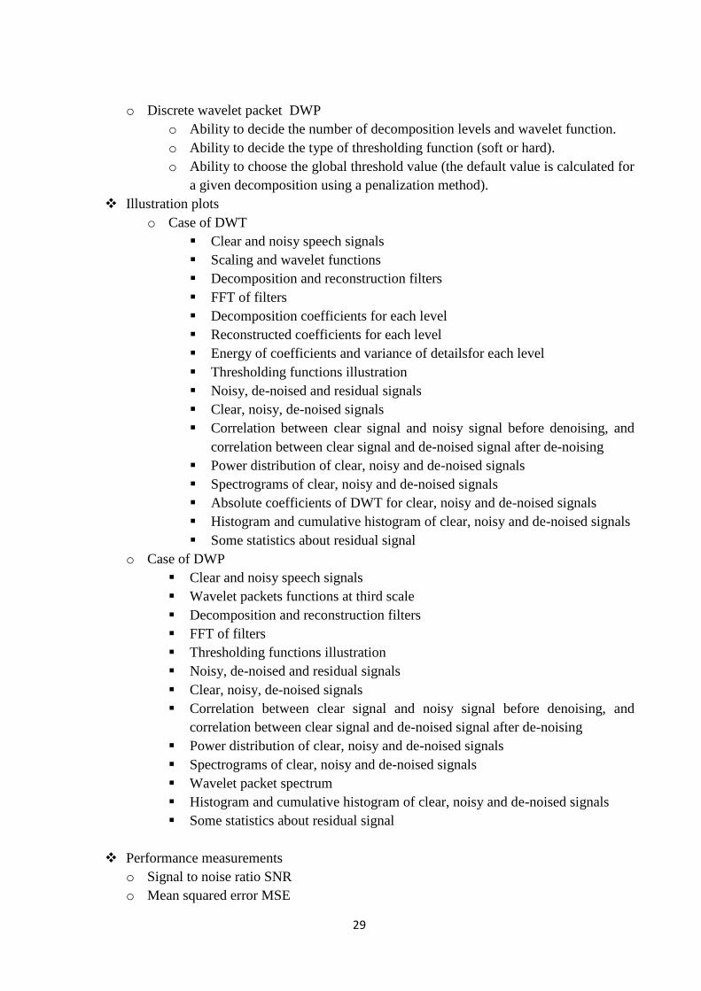
o Discrete wavelet packet DWPo Ability to decide the number of decomposition levels and wavelet function.o Ability to decide the type of thresholding function (soft or hard).o Ability to choose the global threshold value (the default value is calculated for

a given decomposition using a penalization method). Illustration plots

o Case of DWT Clear and noisy speech signals Scaling and wavelet functions Decomposition and reconstruction filters FFT of filters Decomposition coefficients for each level Reconstructed coefficients for each level Energy of coefficients and variance of detailsfor each level Thresholding functions illustration Noisy, de-noised and residual signals Clear, noisy, de-noised signals Correlation between clear signal and noisy signal before denoising, and

correlation between clear signal and de-noised signal after de-noising Power distribution of clear, noisy and de-noised signals Spectrograms of clear, noisy and de-noised signals Absolute coefficients of DWT for clear, noisy and de-noised signals Histogram and cumulative histogram of clear, noisy and de-noised signals Some statistics about residual signal

o Case of DWP Clear and noisy speech signals Wavelet packets functions at third scale Decomposition and reconstruction filters FFT of filters Thresholding functions illustration Noisy, de-noised and residual signals Clear, noisy, de-noised signals Correlation between clear signal and noisy signal before denoising, and

correlation between clear signal and de-noised signal after de-noising Power distribution of clear, noisy and de-noised signals Spectrograms of clear, noisy and de-noised signals Wavelet packet spectrum Histogram and cumulative histogram of clear, noisy and de-noised signals Some statistics about residual signal

Performance measurementso Signal to noise ratio SNRo Mean squared error MSE

30

4.1.2 Illustrative example

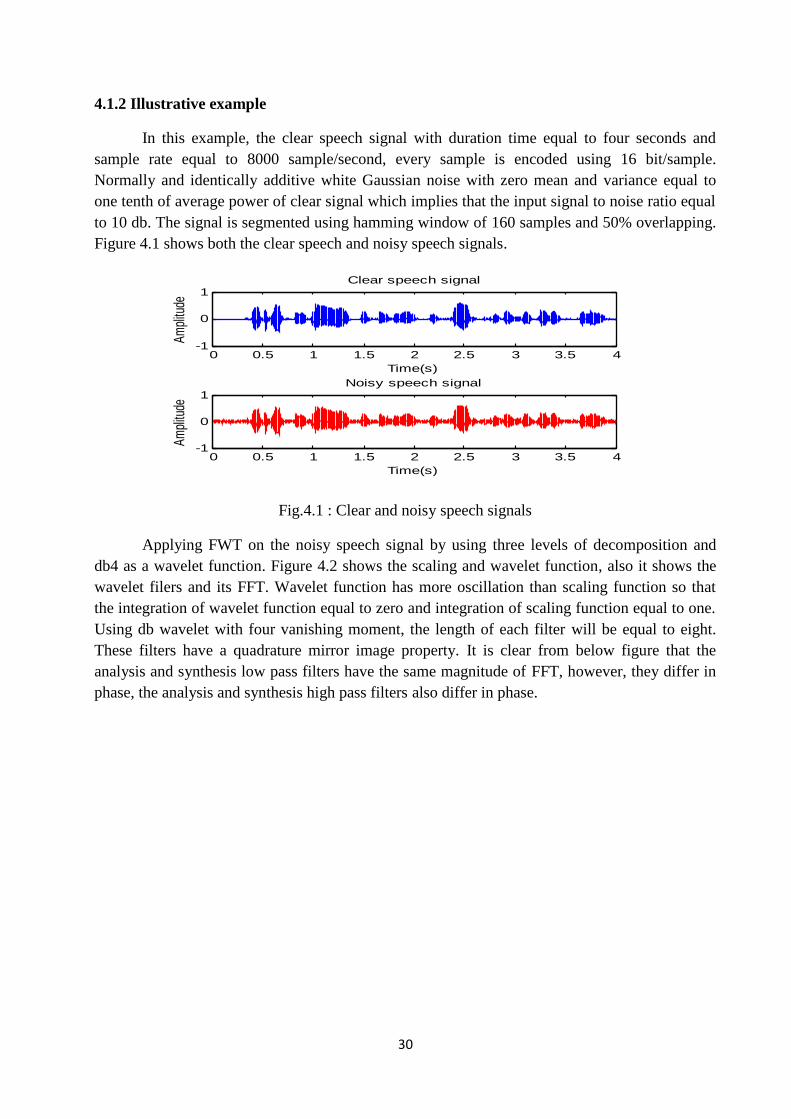
In this example, the clear speech signal with duration time equal to four seconds andsample rate equal to 8000 sample/second, every sample is encoded using 16 bit/sample.Normally and identically additive white Gaussian noise with zero mean and variance equal toone tenth of average power of clear signal which implies that the input signal to noise ratio equalto 10 db. The signal is segmented using hamming window of 160 samples and 50% overlapping.Figure 4.1 shows both the clear speech and noisy speech signals.

Fig.4.1 : Clear and noisy speech signals

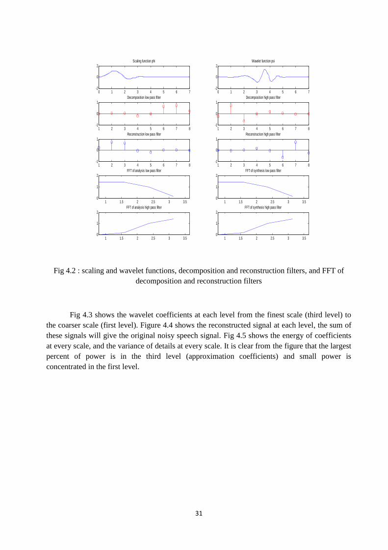
Applying FWT on the noisy speech signal by using three levels of decomposition anddb4 as a wavelet function. Figure 4.2 shows the scaling and wavelet function, also it shows thewavelet filers and its FFT. Wavelet function has more oscillation than scaling function so thatthe integration of wavelet function equal to zero and integration of scaling function equal to one.Using db wavelet with four vanishing moment, the length of each filter will be equal to eight.These filters have a quadrature mirror image property. It is clear from below figure that theanalysis and synthesis low pass filters have the same magnitude of FFT, however, they differ inphase, the analysis and synthesis high pass filters also differ in phase.

0 0.5 1 1.5 2 2.5 3 3.5 4-1

0

1

Time(s)

Ampli

tude

Clear speech signal

0 0.5 1 1.5 2 2.5 3 3.5 4-1

0

1

Time(s)

Ampli

tude

Noisy speech signal

31

Fig 4.2 : scaling and wavelet functions, decomposition and reconstruction filters, and FFT ofdecomposition and reconstruction filters

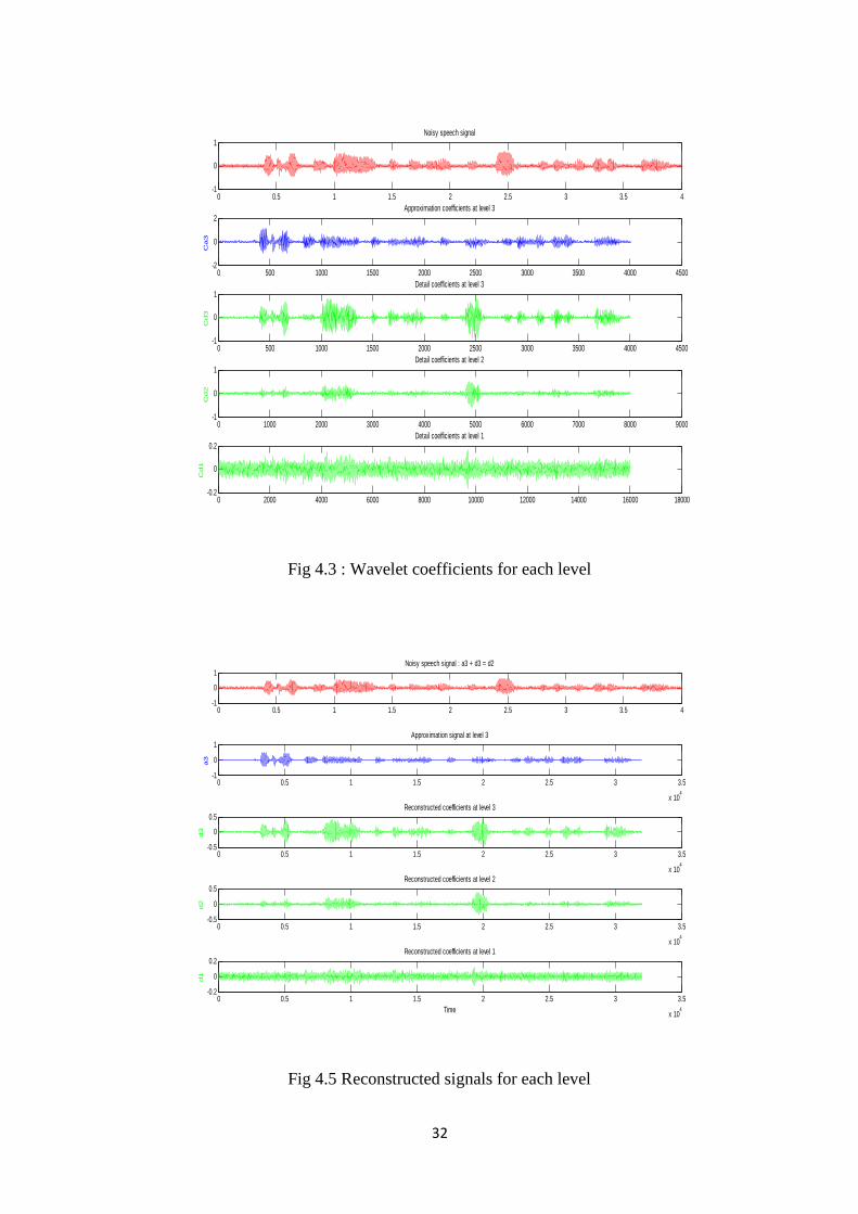
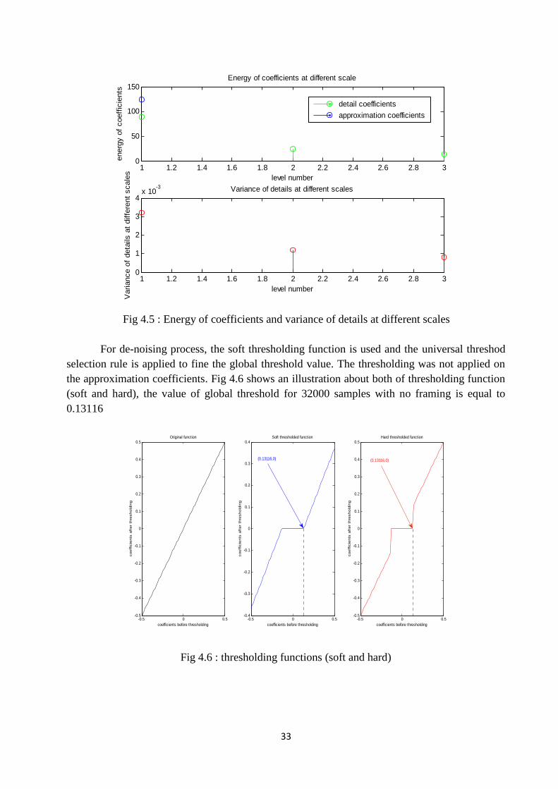
Fig 4.3 shows the wavelet coefficients at each level from the finest scale (third level) tothe coarser scale (first level). Figure 4.4 shows the reconstructed signal at each level, the sum ofthese signals will give the original noisy speech signal. Fig 4.5 shows the energy of coefficientsat every scale, and the variance of details at every scale. It is clear from the figure that the largestpercent of power is in the third level (approximation coefficients) and small power isconcentrated in the first level.

0 1 2 3 4 5 6 7-2

0

2Scaling function phi

0 1 2 3 4 5 6 7-2

0

2Wavelet function psi

1 2 3 4 5 6 7 8-1

0

1Decomposition low pass filter

1 2 3 4 5 6 7 8-1

0

1Decomposition high pass filter

1 2 3 4 5 6 7 8-1

0

1Reconstruction low pass filter

1 2 3 4 5 6 7 8-1

0

1Reconstruction high pass filter

1 1.5 2 2.5 3 3.50

1

2FFT of analysis low pass filter

1 1.5 2 2.5 3 3.50

1

2FFT of synthesis low pass filter

1 1.5 2 2.5 3 3.50

1

2FFT of analysis high pass filter

1 1.5 2 2.5 3 3.50

1

2FFT of synthesis high pass filter

32

Fig 4.3 : Wavelet coefficients for each level

Fig 4.5 Reconstructed signals for each level

0 0.5 1 1.5 2 2.5 3 3.5 4-1

0

1Noisy speech signal

0 500 1000 1500 2000 2500 3000 3500 4000 4500-2

0

2Approximation coefficients at level 3

Ca3

0 500 1000 1500 2000 2500 3000 3500 4000 4500-1

0

1Detail coefficients at level 3

Cd3

0 1000 2000 3000 4000 5000 6000 7000 8000 9000-1

0

1Detail coefficients at level 2

Cd2

0 2000 4000 6000 8000 10000 12000 14000 16000 18000-0.2

0

0.2Detail coefficients at level 1

Cd1

0 0.5 1 1.5 2 2.5 3 3.5 4-1

0

1Noisy speech signal : a3 + d3 = d2

0 0.5 1 1.5 2 2.5 3 3.5

x 104

-1

0

1Approximation signal at level 3

a3

0 0.5 1 1.5 2 2.5 3 3.5

x 104

-0.5

0

0.5Reconstructed coefficients at level 3

d3

0 0.5 1 1.5 2 2.5 3 3.5

x 104

-0.5

0

0.5Reconstructed coefficients at level 2

d2

0 0.5 1 1.5 2 2.5 3 3.5

x 104

-0.2

0

0.2Reconstructed coefficients at level 1

d1

Time

33

Fig 4.5 : Energy of coefficients and variance of details at different scales

For de-noising process, the soft thresholding function is used and the universal threshodselection rule is applied to fine the global threshold value. The thresholding was not applied onthe approximation coefficients. Fig 4.6 shows an illustration about both of thresholding function(soft and hard), the value of global threshold for 32000 samples with no framing is equal to0.13116

Fig 4.6 : thresholding functions (soft and hard)

1 1.2 1.4 1.6 1.8 2 2.2 2.4 2.6 2.8 30

50

100

150Energy of coefficients at different scale

level number

ener

gy o

f co

effic

ient

s

detail coefficients

approximation coefficients

1 1.2 1.4 1.6 1.8 2 2.2 2.4 2.6 2.8 30

1

2

3

4x 10

-3 Variance of details at different scales

level number

Var

ianc

e of

det

ails

at

diff

eren

t sc

ales

-0.5 0 0.5-0.5

-0.4

-0.3

-0.2

-0.1

0

0.1

0.2

0.3

0.4

0.5Original function

coefficients before thresholding

coeff

icie

nts

aft

er

thre

shold

ing

-0.5 0 0.5-0.4

-0.3

-0.2

-0.1

0

0.1

0.2

0.3

0.4Soft thresholded function

(0.13116,0)

coefficients before thresholding

coeff

icie

nts

aft

er

thre

shold

ing

-0.5 0 0.5-0.5

-0.4

-0.3

-0.2

-0.1

0

0.1

0.2

0.3

0.4

0.5Hard thresholded function

(0.13116,0)

coefficients before thresholding

coeff

icie

nts

aft

er

thre

shold

ing

34

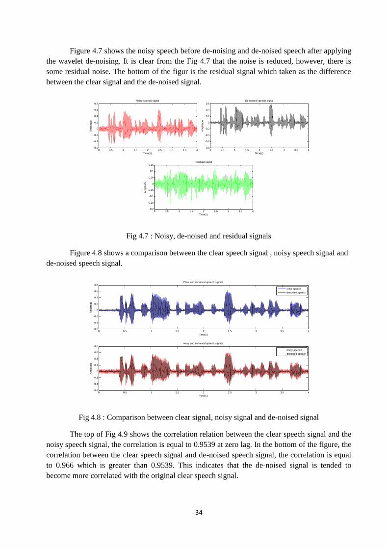
Figure 4.7 shows the noisy speech before de-noising and de-noised speech after applyingthe wavelet de-noising. It is clear from the Fig 4.7 that the noise is reduced, however, there issome residual noise. The bottom of the figur is the residual signal which taken as the differencebetween the clear signal and the de-noised signal.

Fig 4.7 : Noisy, de-noised and residual signals

Figure 4.8 shows a comparison between the clear speech signal , noisy speech signal andde-noised speech signal.

Fig 4.8 : Comparison between clear signal, noisy signal and de-noised signal

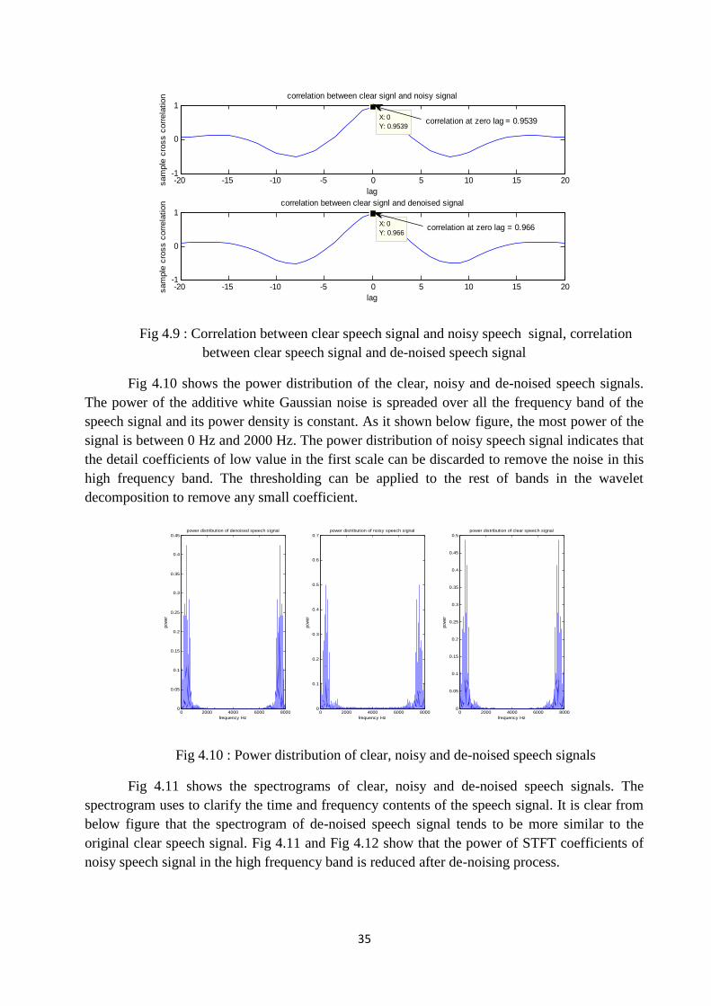
The top of Fig 4.9 shows the correlation relation between the clear speech signal and thenoisy speech signal, the correlation is equal to 0.9539 at zero lag. In the bottom of the figure, thecorrelation between the clear speech signal and de-noised speech signal, the correlation is equalto 0.966 which is greater than 0.9539. This indicates that the de-noised signal is tended tobecome more correlated with the original clear speech signal.

0 0.5 1 1.5 2 2.5 3 3.5 4-0.6

-0.4

-0.2

0

0.2

0.4

0.6

0.8

Time(s)

Am

plitu

de

Noisy speech signal

0 0.5 1 1.5 2 2.5 3 3.5 4-0.8

-0.6

-0.4

-0.2

0

0.2

0.4

0.6

Time(s)

Am

plitu

de

De-noised speech signal

0 0.5 1 1.5 2 2.5 3 3.5 4-0.2

-0.15

-0.1

-0.05

0

0.05

0.1

0.15

Time(s)

Am

plitu

de

Residual signal

0 0.5 1 1.5 2 2.5 3 3.5 4-0.6

-0.4

-0.2

0

0.2

0.4

0.6

0.8

Time(s)

Am

plitu

de

Clear and denoised speech signals

clear speech

denoised speech

0 0.5 1 1.5 2 2.5 3 3.5 4-0.6

-0.4

-0.2

0

0.2

0.4

0.6

0.8

Time(s)

Am

plitu

de

noisy and denoised speech signals

noisy speech

denoised speech

35

Fig 4.9 : Correlation between clear speech signal and noisy speech signal, correlationbetween clear speech signal and de-noised speech signal

Fig 4.10 shows the power distribution of the clear, noisy and de-noised speech signals.The power of the additive white Gaussian noise is spreaded over all the frequency band of thespeech signal and its power density is constant. As it shown below figure, the most power of thesignal is between 0 Hz and 2000 Hz. The power distribution of noisy speech signal indicates thatthe detail coefficients of low value in the first scale can be discarded to remove the noise in thishigh frequency band. The thresholding can be applied to the rest of bands in the waveletdecomposition to remove any small coefficient.

Fig 4.10 : Power distribution of clear, noisy and de-noised speech signals

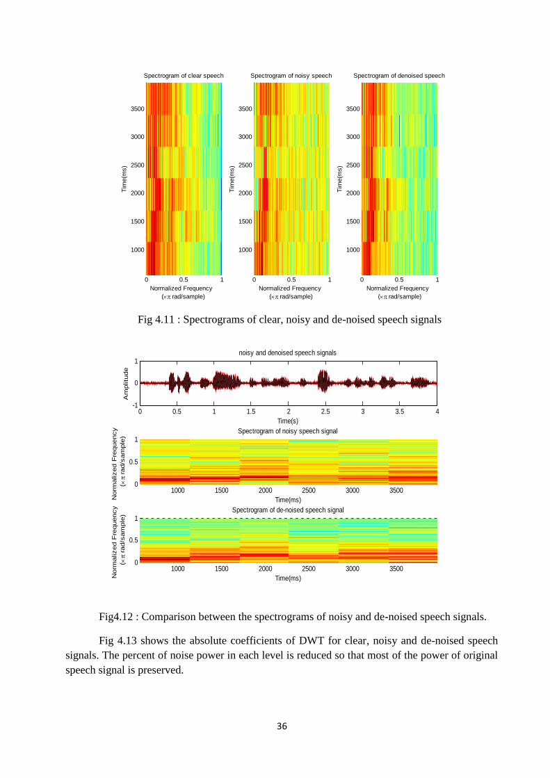
Fig 4.11 shows the spectrograms of clear, noisy and de-noised speech signals. Thespectrogram uses to clarify the time and frequency contents of the speech signal. It is clear frombelow figure that the spectrogram of de-noised speech signal tends to be more similar to theoriginal clear speech signal. Fig 4.11 and Fig 4.12 show that the power of STFT coefficients ofnoisy speech signal in the high frequency band is reduced after de-noising process.

-20 -15 -10 -5 0 5 10 15 20-1

0

1X: 0Y: 0.9539

lag

sam

ple

cros

s co

rrel

atio

n correlation between clear signl and noisy signal

-20 -15 -10 -5 0 5 10 15 20-1

0

1X: 0Y: 0.966

lag

sam

ple

cros

s co

rrel

atio

n correlation between clear signl and denoised signal

correlation at zero lag = 0.9539

correlation at zero lag = 0.966

0 2000 4000 6000 80000

0.05

0.1

0.15

0.2

0.25

0.3

0.35

0.4

0.45

frequency Hz

pow

er

power distribution of denoised speech signal

0 2000 4000 6000 80000

0.1

0.2

0.3

0.4

0.5

0.6

0.7

frequency Hz

pow

er

power distribution of noisy speech signal

0 2000 4000 6000 80000

0.05

0.1

0.15

0.2

0.25

0.3

0.35

0.4

0.45

0.5

frequency Hz

pow

er

power distribution of clear speech signal

36

Fig 4.11 : Spectrograms of clear, noisy and de-noised speech signals

Fig4.12 : Comparison between the spectrograms of noisy and de-noised speech signals.

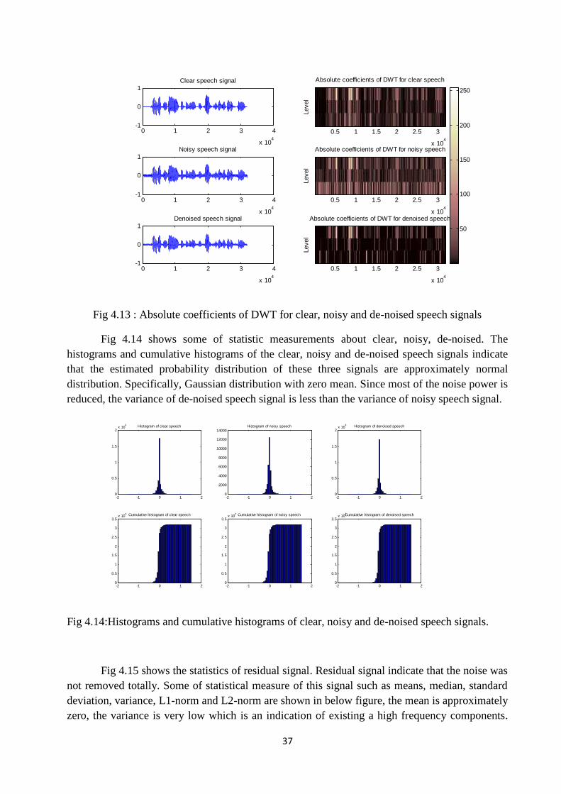
Fig 4.13 shows the absolute coefficients of DWT for clear, noisy and de-noised speechsignals. The percent of noise power in each level is reduced so that most of the power of originalspeech signal is preserved.

0 0.5 1

1000

1500

2000

2500

3000

3500

Spectrogram of clear speech

Normalized Frequency( rad/sample)

Tim

e(m

s)

0 0.5 1

1000

1500

2000

2500

3000

3500

Spectrogram of noisy speech

Normalized Frequency( rad/sample)

Tim

e(m

s)

0 0.5 1

1000

1500

2000

2500

3000

3500

Spectrogram of denoised speech

Normalized Frequency ( rad/sample)

Tim

e(m

s)

0 0.5 1 1.5 2 2.5 3 3.5 4-1

0

1

Time(s)

Am

plit

ude

noisy and denoised speech signals

1000 1500 2000 2500 3000 35000

0.5

1

Time(ms)

Spectrogram of noisy speech signal

Norm

aliz

ed F

requency

(

rad/s

am

ple

)

1000 1500 2000 2500 3000 35000

0.5

1

Time(ms)

Spectrogram of de-noised speech signal

Norm

aliz

ed F

requency

(

rad/s

am

ple

)

37

Fig 4.13 : Absolute coefficients of DWT for clear, noisy and de-noised speech signals

Fig 4.14 shows some of statistic measurements about clear, noisy, de-noised. Thehistograms and cumulative histograms of the clear, noisy and de-noised speech signals indicatethat the estimated probability distribution of these three signals are approximately normaldistribution. Specifically, Gaussian distribution with zero mean. Since most of the noise power isreduced, the variance of de-noised speech signal is less than the variance of noisy speech signal.

Fig 4.14:Histograms and cumulative histograms of clear, noisy and de-noised speech signals.

Fig 4.15 shows the statistics of residual signal. Residual signal indicate that the noise wasnot removed totally. Some of statistical measure of this signal such as means, median, standarddeviation, variance, L1-norm and L2-norm are shown in below figure, the mean is approximatelyzero, the variance is very low which is an indication of existing a high frequency components.

0 1 2 3 4

x 104

-1

0

1Clear speech signal Absolute coefficients of DWT for clear speech

Leve

l

0.5 1 1.5 2 2.5 3

x 104

0 1 2 3 4

x 104

-1

0

1Noisy speech signal Absolute coefficients of DWT for noisy speech

Leve

l

0.5 1 1.5 2 2.5 3

x 104

0 1 2 3 4

x 104

-1

0

1Denoised speech signal Absolute coefficients of DWT for denoised speech

Leve

l

0.5 1 1.5 2 2.5 3

x 104

50

100

150

200

250

-2 -1 0 1 20

0.5

1

1.5

2x 10

4 Histogram of clear speech

-2 -1 0 1 20

0.5

1

1.5

2

2.5

3

3.5x 10

4 Cumulative histogram of clear speech

-2 -1 0 1 20

2000

4000

6000

8000

10000

12000

14000Histogram of noisy speech

-2 -1 0 1 20

0.5

1

1.5

2

2.5

3

3.5x 10

4 Cumulative histogram of noisy speech

-2 -1 0 1 20

0.5

1

1.5

2x 10

4 Histogram of denoised speech

-2 -1 0 1 20

0.5

1

1.5

2

2.5

3

3.5x 10

4Cumulative histogram of denoised speech

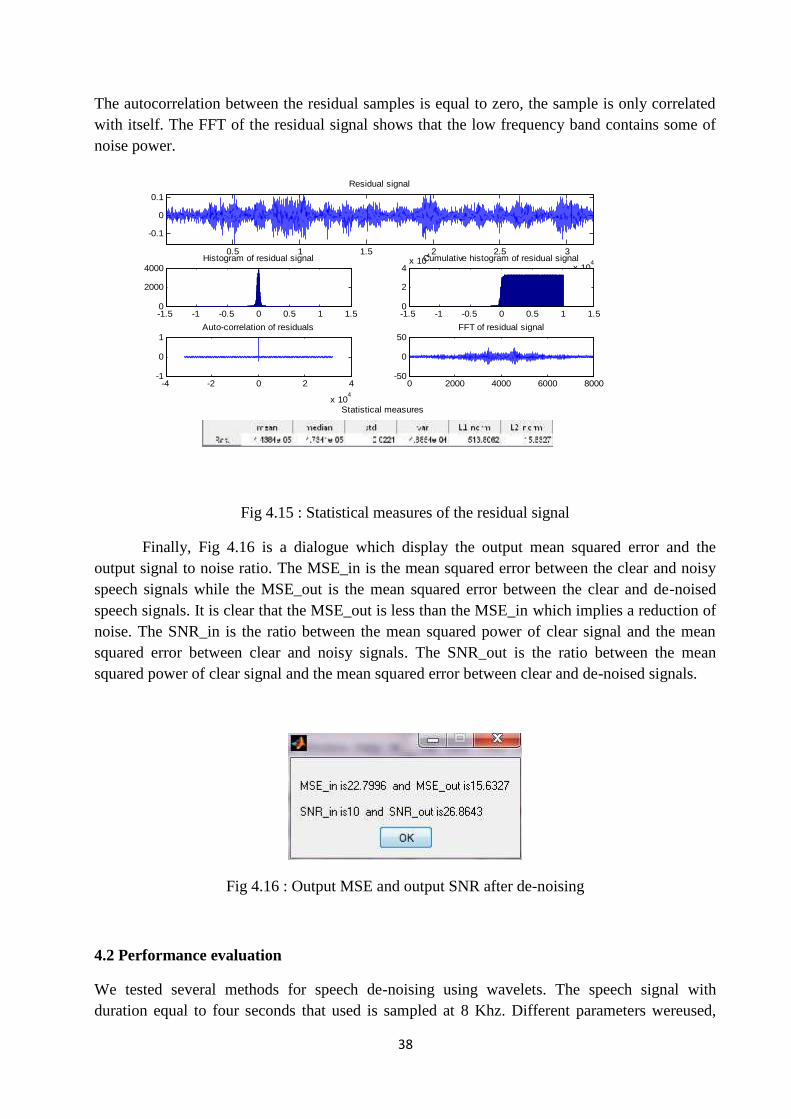
38

The autocorrelation between the residual samples is equal to zero, the sample is only correlatedwith itself. The FFT of the residual signal shows that the low frequency band contains some ofnoise power.

Fig 4.15 : Statistical measures of the residual signal

Finally, Fig 4.16 is a dialogue which display the output mean squared error and theoutput signal to noise ratio. The MSE_in is the mean squared error between the clear and noisyspeech signals while the MSE_out is the mean squared error between the clear and de-noisedspeech signals. It is clear that the MSE_out is less than the MSE_in which implies a reduction ofnoise. The SNR_in is the ratio between the mean squared power of clear signal and the meansquared error between clear and noisy signals. The SNR_out is the ratio between the meansquared power of clear signal and the mean squared error between clear and de-noised signals.

Fig 4.16 : Output MSE and output SNR after de-noising

4.2 Performance evaluation

We tested several methods for speech de-noising using wavelets. The speech signal withduration equal to four seconds that used is sampled at 8 Khz. Different parameters wereused,

0.5 1 1.5 2 2.5 3

x 104

-0.1

0

0.1

Residual signal

-1.5 -1 -0.5 0 0.5 1 1.50

2000

4000Histogram of residual signal

-1.5 -1 -0.5 0 0.5 1 1.50

2

4x 10

4Cumulative histogram of residual signal

-4 -2 0 2 4

x 104

-1

0

1Auto-correlation of residuals

0 2000 4000 6000 8000-50

0

50FFT of residual signal

Statistical measures

39

some of them are fixed and other was changed to get information about the performance of thesemethods. The performance measure that we used is the output signal to noise ratio so that it isconsidered as a dependent variable for all tests.In the following subsections we show the resultsfrom these tests .

4.2.1 Global thresholding method

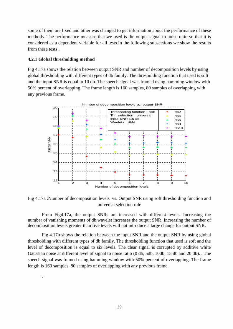
Fig 4.17a shows the relation between output SNR and number of decomposition levels by usingglobal thresholding with different types of db family. The thresholding function that used is softand the input SNR is equal to 10 db. The speech signal was framed using hamming window with50% percent of overlapping. The frame length is 160 samples, 80 samples of overlapping withany previous frame.

Fig 4.17a :Number of decomposition levels vs. Output SNR using soft thresholding function anduniversal selection rule

From Fig4.17a, the output SNRs are increased with different levels. Increasing thenumber of vanishing moments of db wavelet increases the output SNR. Increasing the number ofdecomposition levels greater than five levels will not introduce a large change for output SNR.

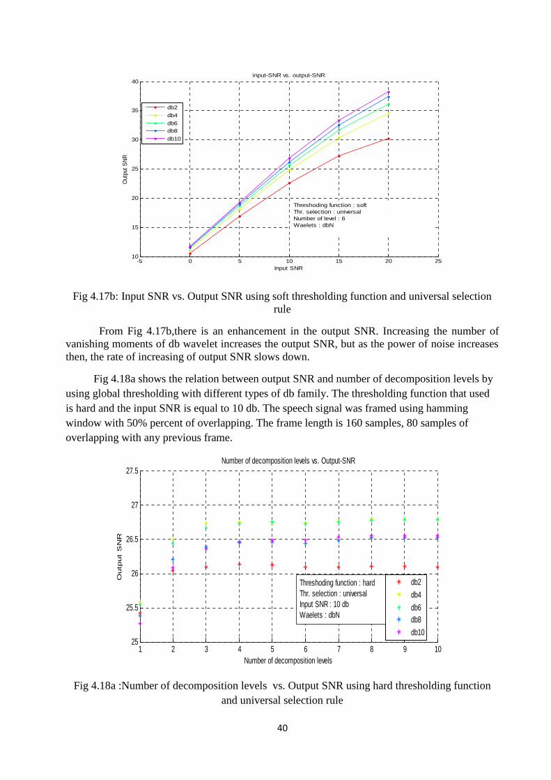
Fig 4.17b shows the relation between the input SNR and the output SNR by using globalthresholding with different types of db family. The thresholding function that used is soft and thelevel of decomposition is equal to six levels. The clear signal is corrupted by additive whiteGaussian noise at different level of signal to noise ratio (0 db, 5db, 10db, 15 db and 20 db). . Thespeech signal was framed using hamming window with 50% percent of overlapping. The framelength is 160 samples, 80 samples of overlapping with any previous frame.

.

1 2 3 4 5 6 7 8 9 1022

23

24

25

26

27

28

29

30

Number of decomposition levels

Outp

ut S

NR

Nnmber of decomposition levels vs. output-SNR

db2

db4

db6db8

db10

Threshoding function : softThr. selection : universalInput SNR :10 dbWaelets : dbN

40

Fig 4.17b: Input SNR vs. Output SNR using soft thresholding function and universal selectionrule

From Fig 4.17b,there is an enhancement in the output SNR. Increasing the number ofvanishing moments of db wavelet increases the output SNR, but as the power of noise increasesthen, the rate of increasing of output SNR slows down.

Fig 4.18a shows the relation between output SNR and number of decomposition levels byusing global thresholding with different types of db family. The thresholding function that usedis hard and the input SNR is equal to 10 db. The speech signal was framed using hammingwindow with 50% percent of overlapping. The frame length is 160 samples, 80 samples ofoverlapping with any previous frame.

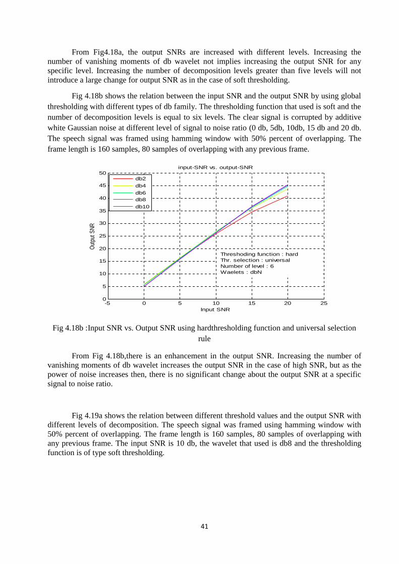
Fig 4.18a :Number of decomposition levels vs. Output SNR using hard thresholding functionand universal selection rule

-5 0 5 10 15 20 2510

15

20

25

30

35

40

Input SNR

Out

put S

NR

input-SNR vs. output-SNR

db2

db4

db6db8

db10

Threshoding function : softThr. selection : universalNumber of level : 6Waelets : dbN

1 2 3 4 5 6 7 8 9 1025

25.5

26

26.5

27

27.5

Number of decomposition levels

Outp

ut

SN

R

Number of decomposition levels vs. Output-SNR

db2

db4

db6db8

db10

Threshoding function : hardThr. selection : universalInput SNR : 10 dbWaelets : dbN

41

From Fig4.18a, the output SNRs are increased with different levels. Increasing thenumber of vanishing moments of db wavelet not implies increasing the output SNR for anyspecific level. Increasing the number of decomposition levels greater than five levels will notintroduce a large change for output SNR as in the case of soft thresholding.

Fig 4.18b shows the relation between the input SNR and the output SNR by using globalthresholding with different types of db family. The thresholding function that used is soft and thenumber of decomposition levels is equal to six levels. The clear signal is corrupted by additivewhite Gaussian noise at different level of signal to noise ratio (0 db, 5db, 10db, 15 db and 20 db.The speech signal was framed using hamming window with 50% percent of overlapping. Theframe length is 160 samples, 80 samples of overlapping with any previous frame.

Fig 4.18b :Input SNR vs. Output SNR using hardthresholding function and universal selectionrule

From Fig 4.18b,there is an enhancement in the output SNR. Increasing the number ofvanishing moments of db wavelet increases the output SNR in the case of high SNR, but as thepower of noise increases then, there is no significant change about the output SNR at a specificsignal to noise ratio.

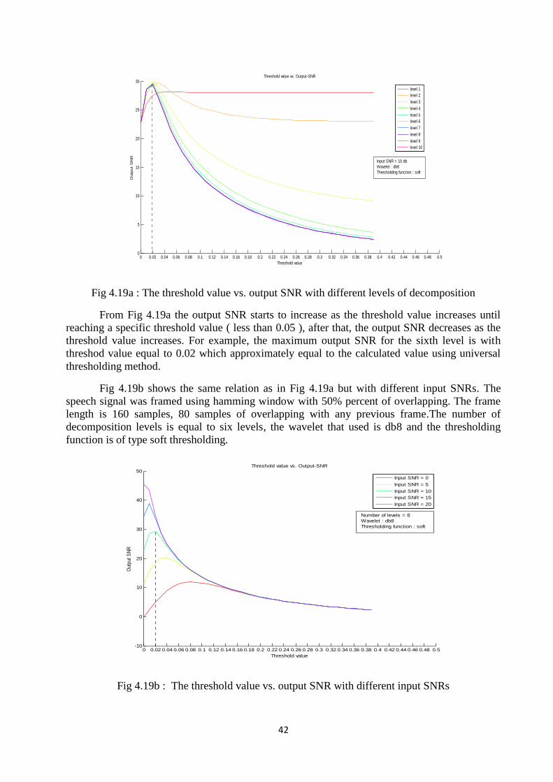
Fig 4.19a shows the relation between different threshold values and the output SNR withdifferent levels of decomposition. The speech signal was framed using hamming window with50% percent of overlapping. The frame length is 160 samples, 80 samples of overlapping withany previous frame. The input SNR is 10 db, the wavelet that used is db8 and the thresholdingfunction is of type soft thresholding.

-5 0 5 10 15 20 250

5

10

15

20

25

30

35

40

45

50

Input SNR

Out

put S

NR

input-SNR vs. output-SNR

db2

db4

db6db8

db10

Threshoding function : hardThr. selection : universalNumber of level : 6Waelets : dbN

42

Fig 4.19a : The threshold value vs. output SNR with different levels of decomposition

From Fig 4.19a the output SNR starts to increase as the threshold value increases untilreaching a specific threshold value ( less than 0.05 ), after that, the output SNR decreases as thethreshold value increases. For example, the maximum output SNR for the sixth level is withthreshod value equal to 0.02 which approximately equal to the calculated value using universalthresholding method.

Fig 4.19b shows the same relation as in Fig 4.19a but with different input SNRs. Thespeech signal was framed using hamming window with 50% percent of overlapping. The framelength is 160 samples, 80 samples of overlapping with any previous frame.The number ofdecomposition levels is equal to six levels, the wavelet that used is db8 and the thresholdingfunction is of type soft thresholding.

Fig 4.19b : The threshold value vs. output SNR with different input SNRs

0 0.02 0.04 0.06 0.08 0.1 0.12 0.14 0.16 0.18 0.2 0.22 0.24 0.26 0.28 0.3 0.32 0.34 0.36 0.38 0.4 0.42 0.44 0.46 0.48 0.50

5

10

15

20

25

30Threshold value vs. Output-SNR

Threshold value

Outp

ut

SN

R

level 1level 2

level 3

level 4

level 5level 6

level 7

level 8

level 9level 10

Input SNR = 10 db Wavelet : db8 Thresholding function : soft

0 0.02 0.04 0.06 0.08 0.1 0.12 0.14 0.16 0.18 0.2 0.22 0.24 0.26 0.28 0.3 0.32 0.34 0.36 0.38 0.4 0.42 0.44 0.46 0.48 0.5-10

0

10

20

30

40

50Threshold value vs. Output-SNR

Threshold value

Out

put S

NR

Input SNR = 0

Input SNR = 5

Input SNR = 10Input SNR = 15

Input SNR = 20

Number of levels = 6 Wavelet : db8 Thresholding function : soft

43

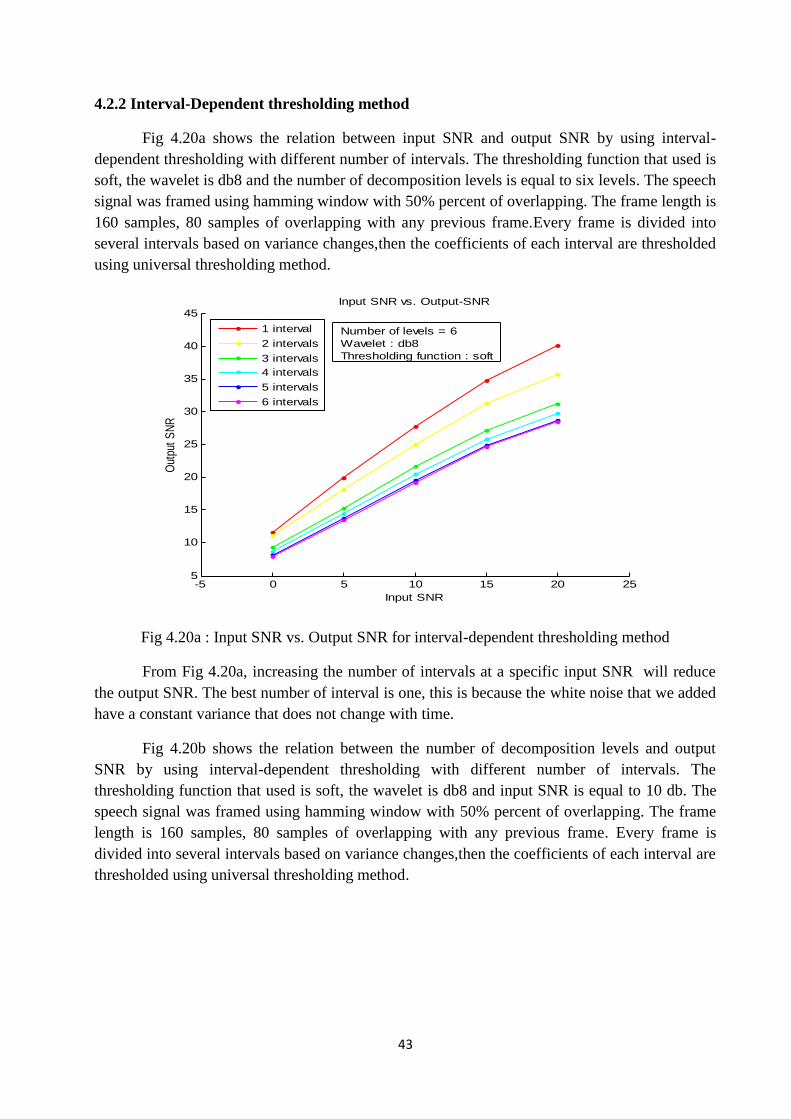
4.2.2 Interval-Dependent thresholding method

Fig 4.20a shows the relation between input SNR and output SNR by using interval-dependent thresholding with different number of intervals. The thresholding function that used issoft, the wavelet is db8 and the number of decomposition levels is equal to six levels. The speechsignal was framed using hamming window with 50% percent of overlapping. The frame length is160 samples, 80 samples of overlapping with any previous frame.Every frame is divided intoseveral intervals based on variance changes,then the coefficients of each interval are thresholdedusing universal thresholding method.

Fig 4.20a : Input SNR vs. Output SNR for interval-dependent thresholding method

From Fig 4.20a, increasing the number of intervals at a specific input SNR will reducethe output SNR. The best number of interval is one, this is because the white noise that we addedhave a constant variance that does not change with time.

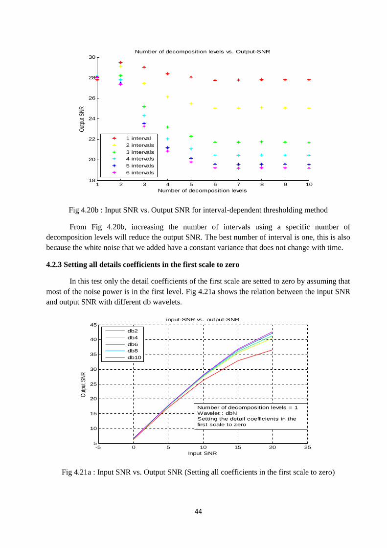
Fig 4.20b shows the relation between the number of decomposition levels and outputSNR by using interval-dependent thresholding with different number of intervals. Thethresholding function that used is soft, the wavelet is db8 and input SNR is equal to 10 db. Thespeech signal was framed using hamming window with 50% percent of overlapping. The framelength is 160 samples, 80 samples of overlapping with any previous frame. Every frame isdivided into several intervals based on variance changes,then the coefficients of each interval arethresholded using universal thresholding method.

-5 0 5 10 15 20 255

10

15

20

25

30

35

40

45

Input SNR

Out

put S

NR

Input SNR vs. Output-SNR

1 interval

2 intervals

3 intervals4 intervals

5 intervals

6 intervals

Number of levels = 6Wavelet : db8Thresholding function : soft

44

Fig 4.20b : Input SNR vs. Output SNR for interval-dependent thresholding method

From Fig 4.20b, increasing the number of intervals using a specific number ofdecomposition levels will reduce the output SNR. The best number of interval is one, this is alsobecause the white noise that we added have a constant variance that does not change with time.

4.2.3 Setting all details coefficients in the first scale to zero

In this test only the detail coefficients of the first scale are setted to zero by assuming thatmost of the noise power is in the first level. Fig 4.21a shows the relation between the input SNRand output SNR with different db wavelets.

Fig 4.21a : Input SNR vs. Output SNR (Setting all coefficients in the first scale to zero)

1 2 3 4 5 6 7 8 9 1018

20

22

24

26

28

30

Number of decomposition levels

Outp

ut S

NR

Number of decomposition levels vs. Output-SNR

1 interval

2 intervals

3 intervals4 intervals

5 intervals

6 intervals

-5 0 5 10 15 20 255

10

15

20

25

30

35

40

45

Input SNR

Outp

ut S

NR

input-SNR vs. output-SNR

db2

db4

db6db8

db10

Number of decomposition levels = 1Wavelet : dbNSetting the detail coefficients in thefirst scale to zero

45

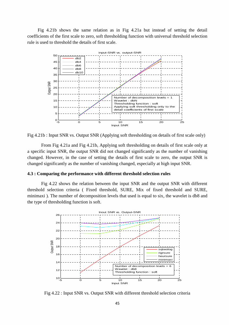
Fig 4.21b shows the same relation as in Fig 4.21a but instead of setting the detailcoefficients of the first scale to zero, soft thresholding function with universal threshold selectionrule is used to threshold the details of first scale.

Fig 4.21b : Input SNR vs. Output SNR (Applying soft thresholding on details of first scale only)

From Fig 4.21a and Fig 4.21b, Applying soft thresholding on details of first scale only ata specific input SNR, the output SNR did not changed significantly as the number of vanishingchanged. However, in the case of setting the details of first scale to zero, the output SNR ischanged significantly as the number of vanishing changed, especially at high input SNR.

4.3 : Comparing the performance with different threshold selection rules

Fig 4.22 shows the relation between the input SNR and the output SNR with differentthreshold selection criteria ( Fixed threshold, SURE, Mix of fixed threshold and SURE,minimaxi ). The number of decomposition levels that used is equal to six, the wavelet is db8 andthe type of thresholding function is soft.

Fig 4.22 : Input SNR vs. Output SNR with different threshold selection criteria

-5 0 5 10 15 20 250

5

10

15

20

25

30

35

40

45

50

Input SNR

Outpu

t SNR

input-SNR vs. output-SNR

db2

db4

db6db8

db10

Number of decomposition levels = 1Wavelet : dbNThresholding function : softApplying soft thresholding only to thedetail coefficients of first scale

-5 0 5 10 15 20 2510

12

14

16

18

20

22

24

26

Input SNR

Outpu

t SNR

Inout SNR vs. Output-SNR

sqtwolog

rigrsureheursure

minimaxi

Number of decomposition levels = 6Wavelet : db8Thresholding function : soft

46

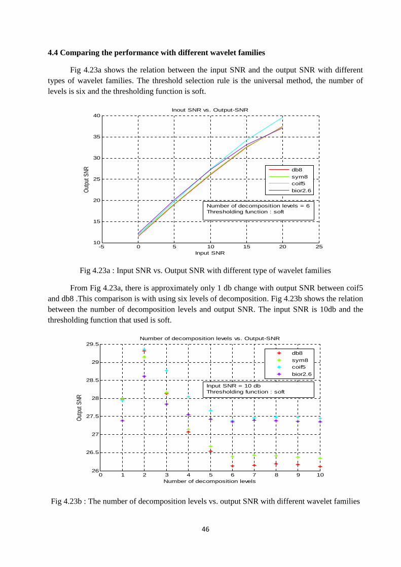
4.4 Comparing the performance with different wavelet families

Fig 4.23a shows the relation between the input SNR and the output SNR with differenttypes of wavelet families. The threshold selection rule is the universal method, the number oflevels is six and the thresholding function is soft.

Fig 4.23a : Input SNR vs. Output SNR with different type of wavelet families

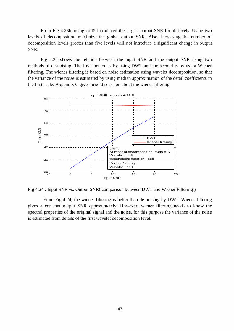
From Fig 4.23a, there is approximately only 1 db change with output SNR between coif5and db8 .This comparison is with using six levels of decomposition. Fig 4.23b shows the relationbetween the number of decomposition levels and output SNR. The input SNR is 10db and thethresholding function that used is soft.

Fig 4.23b : The number of decomposition levels vs. output SNR with different wavelet families

-5 0 5 10 15 20 2510

15

20

25

30

35

40

Input SNR

Outp

ut S

NR

Inout SNR vs. Output-SNR

db8

sym8coif5

bior2.6

Number of decomposition levels = 6Thresholding function : soft

0 1 2 3 4 5 6 7 8 9 1026

26.5

27

27.5

28

28.5

29

29.5

Number of decomposition levels

Outp

ut S

NR

Number of decomposition levels vs. Output-SNR

db8

sym8coif5

bior2.6

Input SNR = 10 dbThresholding function : soft

47

From Fig 4.23b, using coif5 introduced the largest output SNR for all levels. Using twolevels of decomposition maximize the global output SNR. Also, increasing the number ofdecomposition levels greater than five levels will not introduce a significant change in outputSNR.

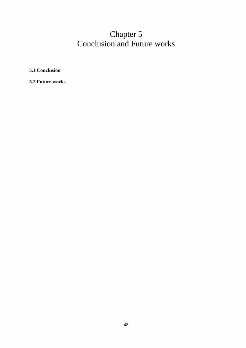
Fig 4.24 shows the relation between the input SNR and the output SNR using twomethods of de-noising. The first method is by using DWT and the second is by using Wienerfiltering. The wiener filtering is based on noise estimation using wavelet decomposition, so thatthe variance of the noise is estimated by using median approximation of the detail coefficients inthe first scale. Appendix C gives brief discussion about the wiener filtering.

Fig 4.24 : Input SNR vs. Output SNR( comparison between DWT and Wiener Filtering )

From Fig 4.24, the wiener filtering is better than de-noising by DWT. Wiener filteringgives a constant output SNR approximately. However, wiener filtering needs to know thespectral properties of the original signal and the noise, for this purpose the variance of the noiseis estimated from details of the first wavelet decomposition level.

-5 0 5 10 15 20 2520

30

40

50

60

70

80

Input SNR

Outp

ut S

NR

input-SNR vs. output-SNR

DWT

Wiener filtering

DWT:Number of decomposition levels = 6Wavelet : db8thresholding function : soft

Wiener filtering:Wavelet : db8

48

Chapter 5Conclusion and Future works

5.1 Conclusion

5.2 Future works

49

5.1 Conclusion

Speech de-noising algorithm using discrete wavelet transform is implemented toeliminate a white noise. As shown in this project the selection of threshold value is an importantparameter for speech enhancement. Using universal thesholding by fixed threshold applied tothreshold the wavelet coefficients introduce an efficient way to remove the additive whiteGaussian noise. Interval dependent method is also used to adapt the threshold value, howeversince the Gaussian noise is stationary and its variance did not change with time this method ismore appropriate to non-white noise. Different parameters were changed to get more optimalchoice of them. This project concentrates on db wavelets and shows that this kind of wavelettends to be an appropriate choice for speech enhancement, Specially, under the assumption thatthe noise is Additive white Gaussian noise. Soft thresholding function is more appropriate forspeech de-noising.

As a comparison with other method of de-noising, Wiener filtering based on the waveletdecomposition for noise estimation. In this method the noise is estimated from the first scale ofwavelet decomposition and this estimation used to apply wiener filtering. The experiment showsthat wiener filtering introduce more enhancement in output SNR compared with de-noising usingglobal thresholding in the discrete wavelet domain.

5.2 Future works

The project concentrated on the additive white Gaussian noise, and this work can beextended to a non-white noise. There are many wavelet families that could be tested for speechenhancement. There are many other variations about thresholding function that could also betested. There are many other techniques to adapt the threshold value which could be tested.Using other filtering techniques with wavelet de-noising method to get more optimal filtering.

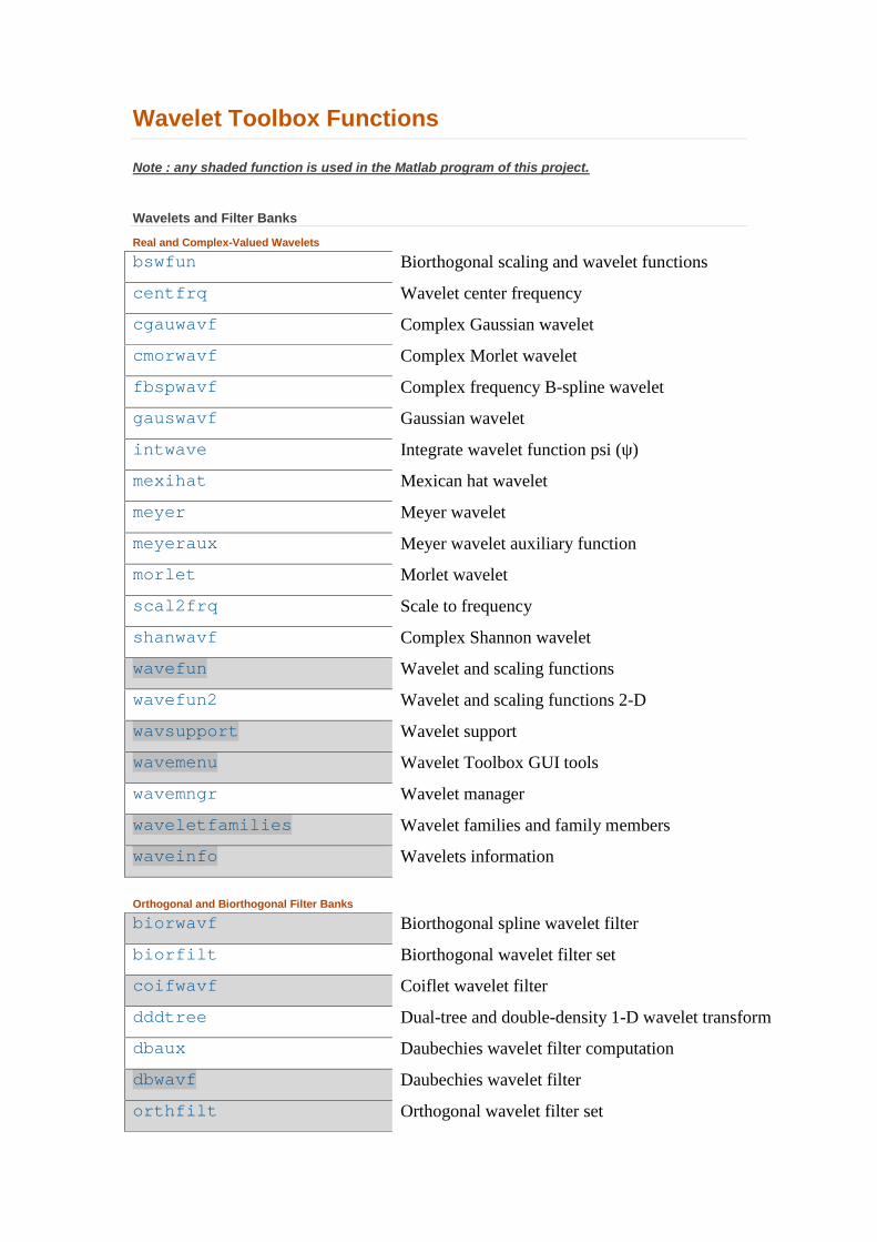
Wavelet Toolbox Functions

Note : any shaded function is used in the Matlab program of this project.

Wavelets and Filter Banks

Real and Complex-Valued Wavelets

bswfun Biorthogonal scaling and wavelet functions

centfrq Wavelet center frequency

cgauwavf Complex Gaussian wavelet

cmorwavf Complex Morlet wavelet

fbspwavf Complex frequency B-spline wavelet

gauswavf Gaussian wavelet

intwave Integrate wavelet function psi (ψ)

mexihat Mexican hat wavelet

meyer Meyer wavelet

meyeraux Meyer wavelet auxiliary function

morlet Morlet wavelet

scal2frq Scale to frequency

shanwavf Complex Shannon wavelet

wavefun Wavelet and scaling functions

wavefun2 Wavelet and scaling functions 2-D

wavsupport Wavelet support

wavemenu Wavelet Toolbox GUI tools

wavemngr Wavelet manager

waveletfamilies Wavelet families and family members

waveinfo Wavelets information

Orthogonal and Biorthogonal Filter Banks

biorwavf Biorthogonal spline wavelet filter

biorfilt Biorthogonal wavelet filter set

coifwavf Coiflet wavelet filter

dddtree Dual-tree and double-density 1-D wavelet transform

dbaux Daubechies wavelet filter computation

dbwavf Daubechies wavelet filter

orthfilt Orthogonal wavelet filter set

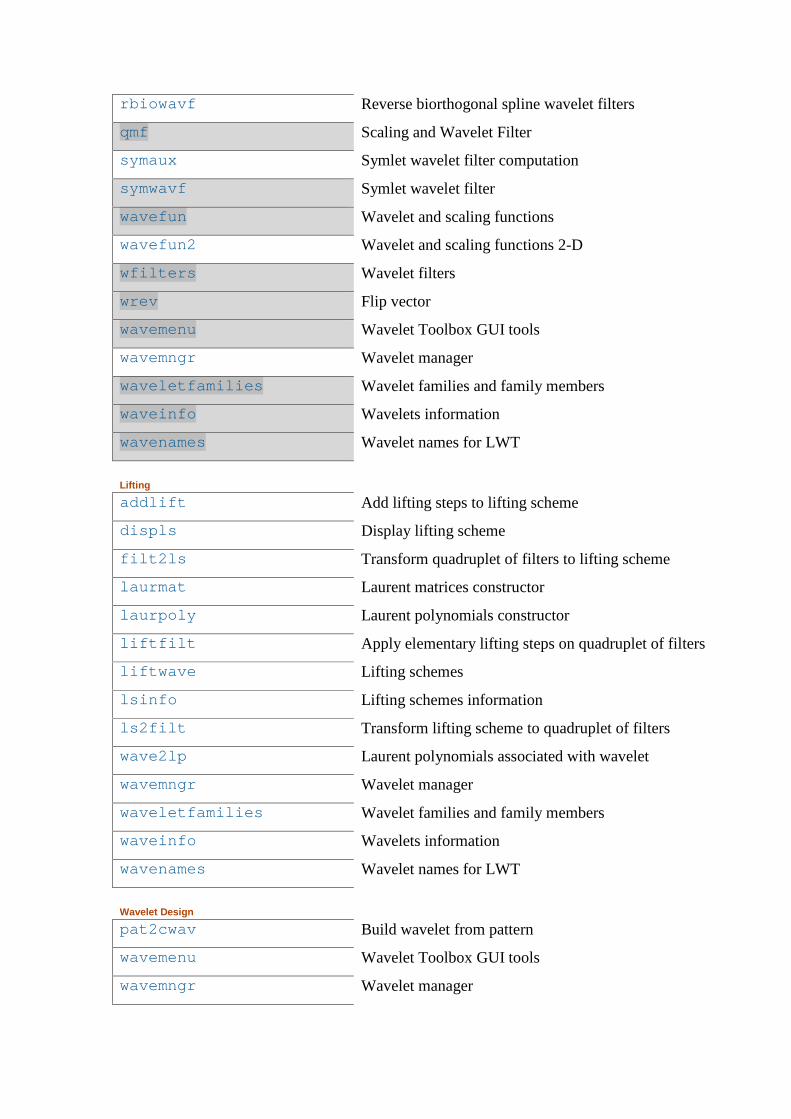
rbiowavf Reverse biorthogonal spline wavelet filters

qmf Scaling and Wavelet Filter

symaux Symlet wavelet filter computation

symwavf Symlet wavelet filter

wavefun Wavelet and scaling functions

wavefun2 Wavelet and scaling functions 2-D

wfilters Wavelet filters

wrev Flip vector

wavemenu Wavelet Toolbox GUI tools

wavemngr Wavelet manager

waveletfamilies Wavelet families and family members

waveinfo Wavelets information

wavenames Wavelet names for LWT

Lifting

addlift Add lifting steps to lifting scheme

displs Display lifting scheme

filt2ls Transform quadruplet of filters to lifting scheme

laurmat Laurent matrices constructor

laurpoly Laurent polynomials constructor

liftfilt Apply elementary lifting steps on quadruplet of filters

liftwave Lifting schemes

lsinfo Lifting schemes information

ls2filt Transform lifting scheme to quadruplet of filters

wave2lp Laurent polynomials associated with wavelet

wavemngr Wavelet manager

waveletfamilies Wavelet families and family members

waveinfo Wavelets information

wavenames Wavelet names for LWT

Wavelet Design

pat2cwav Build wavelet from pattern

wavemenu Wavelet Toolbox GUI tools

wavemngr Wavelet manager

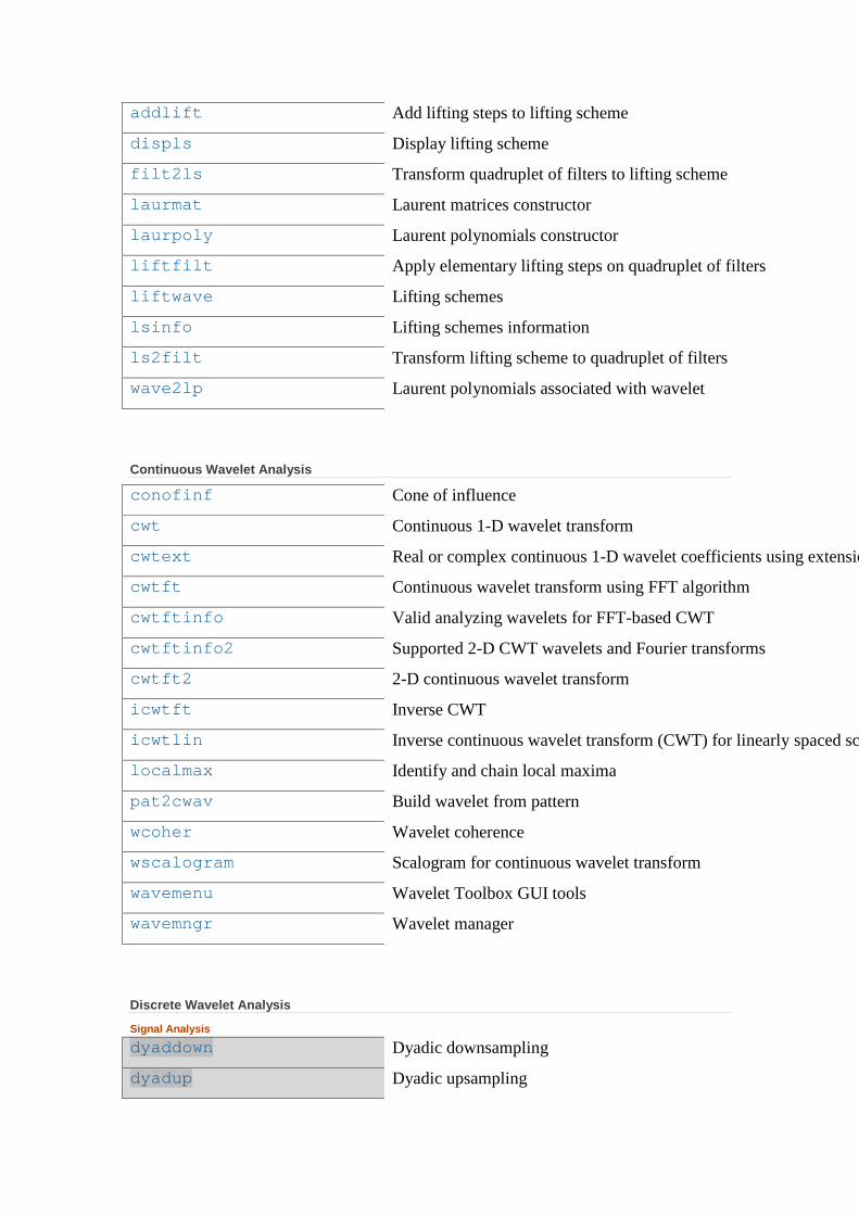
addlift Add lifting steps to lifting scheme

displs Display lifting scheme

filt2ls Transform quadruplet of filters to lifting scheme

laurmat Laurent matrices constructor

laurpoly Laurent polynomials constructor

liftfilt Apply elementary lifting steps on quadruplet of filters

liftwave Lifting schemes

lsinfo Lifting schemes information

ls2filt Transform lifting scheme to quadruplet of filters

wave2lp Laurent polynomials associated with wavelet

Continuous Wavelet Analysis

conofinf Cone of influence

cwt Continuous 1-D wavelet transform

cwtext Real or complex continuous 1-D wavelet coefficients using extension parameters

cwtft Continuous wavelet transform using FFT algorithm

cwtftinfo Valid analyzing wavelets for FFT-based CWT

cwtftinfo2 Supported 2-D CWT wavelets and Fourier transforms

cwtft2 2-D continuous wavelet transform

icwtft Inverse CWT

icwtlin Inverse continuous wavelet transform (CWT) for linearly spaced scales

localmax Identify and chain local maxima

pat2cwav Build wavelet from pattern

wcoher Wavelet coherence

wscalogram Scalogram for continuous wavelet transform

wavemenu Wavelet Toolbox GUI tools

wavemngr Wavelet manager

Discrete Wavelet Analysis

Signal Analysis

dyaddown Dyadic downsampling

dyadup Dyadic upsampling

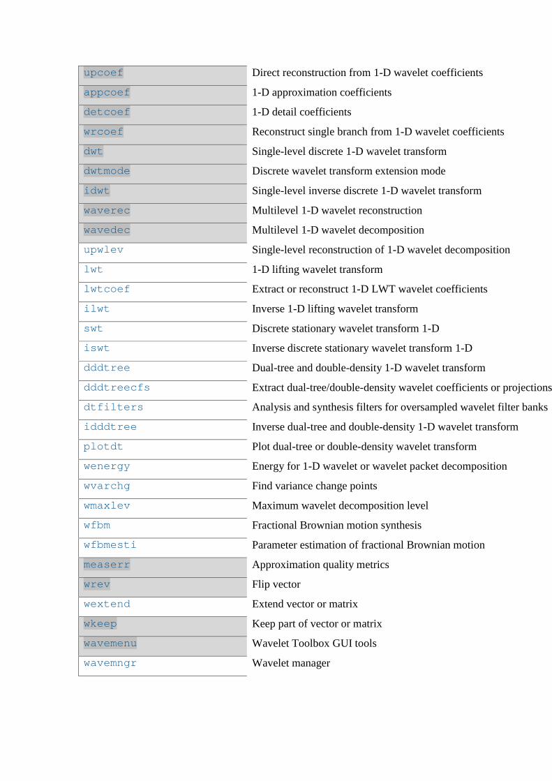
upcoef Direct reconstruction from 1-D wavelet coefficients

appcoef 1-D approximation coefficients

detcoef 1-D detail coefficients

wrcoef Reconstruct single branch from 1-D wavelet coefficients

dwt Single-level discrete 1-D wavelet transform

dwtmode Discrete wavelet transform extension mode

idwt Single-level inverse discrete 1-D wavelet transform

waverec Multilevel 1-D wavelet reconstruction

wavedec Multilevel 1-D wavelet decomposition

upwlev Single-level reconstruction of 1-D wavelet decomposition

lwt 1-D lifting wavelet transform

lwtcoef Extract or reconstruct 1-D LWT wavelet coefficients

ilwt Inverse 1-D lifting wavelet transform

swt Discrete stationary wavelet transform 1-D

iswt Inverse discrete stationary wavelet transform 1-D

dddtree Dual-tree and double-density 1-D wavelet transform

dddtreecfs Extract dual-tree/double-density wavelet coefficients or projections

dtfilters Analysis and synthesis filters for oversampled wavelet filter banks

idddtree Inverse dual-tree and double-density 1-D wavelet transform

plotdt Plot dual-tree or double-density wavelet transform

wenergy Energy for 1-D wavelet or wavelet packet decomposition

wvarchg Find variance change points

wmaxlev Maximum wavelet decomposition level

wfbm Fractional Brownian motion synthesis

wfbmesti Parameter estimation of fractional Brownian motion

measerr Approximation quality metrics

wrev Flip vector

wextend Extend vector or matrix

wkeep Keep part of vector or matrix

wavemenu Wavelet Toolbox GUI tools

wavemngr Wavelet manager

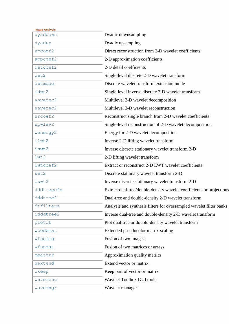
Image Analysis

dyaddown Dyadic downsampling

dyadup Dyadic upsampling

upcoef2 Direct reconstruction from 2-D wavelet coefficients

appcoef2 2-D approximation coefficients

detcoef2 2-D detail coefficients

dwt2 Single-level discrete 2-D wavelet transform

dwtmode Discrete wavelet transform extension mode

idwt2 Single-level inverse discrete 2-D wavelet transform

wavedec2 Multilevel 2-D wavelet decomposition

waverec2 Multilevel 2-D wavelet reconstruction

wrcoef2 Reconstruct single branch from 2-D wavelet coefficients

upwlev2 Single-level reconstruction of 2-D wavelet decomposition

wenergy2 Energy for 2-D wavelet decomposition

ilwt2 Inverse 2-D lifting wavelet transform

iswt2 Inverse discrete stationary wavelet transform 2-D

lwt2 2-D lifting wavelet transform

lwtcoef2 Extract or reconstruct 2-D LWT wavelet coefficients

swt2 Discrete stationary wavelet transform 2-D

iswt2 Inverse discrete stationary wavelet transform 2-D

dddtreecfs Extract dual-tree/double-density wavelet coefficients or projections

dddtree2 Dual-tree and double-density 2-D wavelet transform

dtfilters Analysis and synthesis filters for oversampled wavelet filter banks

idddtree2 Inverse dual-tree and double-density 2-D wavelet transform

plotdt Plot dual-tree or double-density wavelet transform

wcodemat Extended pseudocolor matrix scaling

wfusimg Fusion of two images

wfusmat Fusion of two matrices or arrayz

measerr Approximation quality metrics

wextend Extend vector or matrix

wkeep Keep part of vector or matrix

wavemenu Wavelet Toolbox GUI tools

wavemngr Wavelet manager

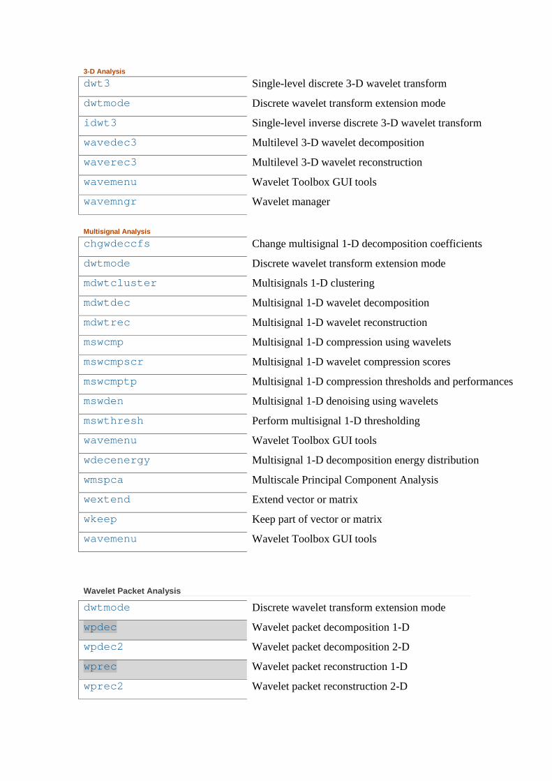
3-D Analysis

dwt3 Single-level discrete 3-D wavelet transform

dwtmode Discrete wavelet transform extension mode

idwt3 Single-level inverse discrete 3-D wavelet transform

wavedec3 Multilevel 3-D wavelet decomposition

waverec3 Multilevel 3-D wavelet reconstruction

wavemenu Wavelet Toolbox GUI tools

wavemngr Wavelet manager

Multisignal Analysis

chgwdeccfs Change multisignal 1-D decomposition coefficients

dwtmode Discrete wavelet transform extension mode

mdwtcluster Multisignals 1-D clustering

mdwtdec Multisignal 1-D wavelet decomposition

mdwtrec Multisignal 1-D wavelet reconstruction

mswcmp Multisignal 1-D compression using wavelets

mswcmpscr Multisignal 1-D wavelet compression scores

mswcmptp Multisignal 1-D compression thresholds and performances

mswden Multisignal 1-D denoising using wavelets

mswthresh Perform multisignal 1-D thresholding

wavemenu Wavelet Toolbox GUI tools

wdecenergy Multisignal 1-D decomposition energy distribution

wmspca Multiscale Principal Component Analysis

wextend Extend vector or matrix

wkeep Keep part of vector or matrix

wavemenu Wavelet Toolbox GUI tools

Wavelet Packet Analysis

dwtmode Discrete wavelet transform extension mode

wpdec Wavelet packet decomposition 1-D

wpdec2 Wavelet packet decomposition 2-D

wprec Wavelet packet reconstruction 1-D

wprec2 Wavelet packet reconstruction 2-D

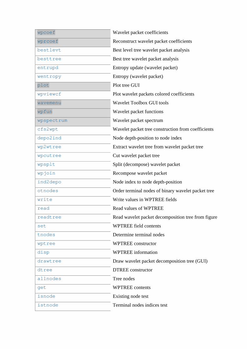
wpcoef Wavelet packet coefficients

wprcoef Reconstruct wavelet packet coefficients

bestlevt Best level tree wavelet packet analysis

besttree Best tree wavelet packet analysis

entrupd Entropy update (wavelet packet)

wentropy Entropy (wavelet packet)

plot Plot tree GUI

wpviewcf Plot wavelet packets colored coefficients

wavemenu Wavelet Toolbox GUI tools

wpfun Wavelet packet functions

wpspectrum Wavelet packet spectrum

cfs2wpt Wavelet packet tree construction from coefficients

depo2ind Node depth-position to node index

wp2wtree Extract wavelet tree from wavelet packet tree

wpcutree Cut wavelet packet tree

wpsplt Split (decompose) wavelet packet

wpjoin Recompose wavelet packet

ind2depo Node index to node depth-position

otnodes Order terminal nodes of binary wavelet packet tree

write Write values in WPTREE fields

read Read values of WPTREE

readtree Read wavelet packet decomposition tree from figure

set WPTREE field contents

tnodes Determine terminal nodes

wptree WPTREE constructor

disp WPTREE information

drawtree Draw wavelet packet decomposition tree (GUI)

dtree DTREE constructor

allnodes Tree nodes

get WPTREE contents

isnode Existing node test

istnode Terminal nodes indices test

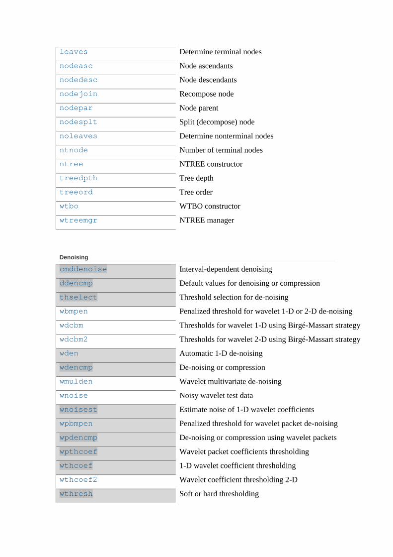
leaves Determine terminal nodes

nodeasc Node ascendants

nodedesc Node descendants

nodejoin Recompose node

nodepar Node parent

nodesplt Split (decompose) node

noleaves Determine nonterminal nodes

ntnode Number of terminal nodes

ntree NTREE constructor

treedpth Tree depth

treeord Tree order

wtbo WTBO constructor

wtreemgr NTREE manager

Denoising

cmddenoise Interval-dependent denoising

ddencmp Default values for denoising or compression

thselect Threshold selection for de-noising

wbmpen Penalized threshold for wavelet 1-D or 2-D de-noising

wdcbm Thresholds for wavelet 1-D using Birgé-Massart strategy

wdcbm2 Thresholds for wavelet 2-D using Birgé-Massart strategy

wden Automatic 1-D de-noising

wdencmp De-noising or compression

wmulden Wavelet multivariate de-noising

wnoise Noisy wavelet test data

wnoisest Estimate noise of 1-D wavelet coefficients

wpbmpen Penalized threshold for wavelet packet de-noising

wpdencmp De-noising or compression using wavelet packets

wpthcoef Wavelet packet coefficients thresholding

wthcoef 1-D wavelet coefficient thresholding

wthcoef2 Wavelet coefficient thresholding 2-D

wthresh Soft or hard thresholding

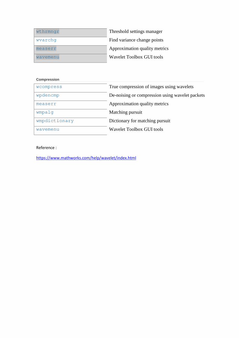
wthrmngr Threshold settings manager

wvarchg Find variance change points

measerr Approximation quality metrics

wavemenu Wavelet Toolbox GUI tools

Compression

wcompress True compression of images using wavelets

wpdencmp De-noising or compression using wavelet packets

measerr Approximation quality metrics

wmpalg Matching pursuit

wmpdictionary Dictionary for matching pursuit

wavemenu Wavelet Toolbox GUI tools

Reference :

https://www.mathworks.com/help/wavelet/index.html

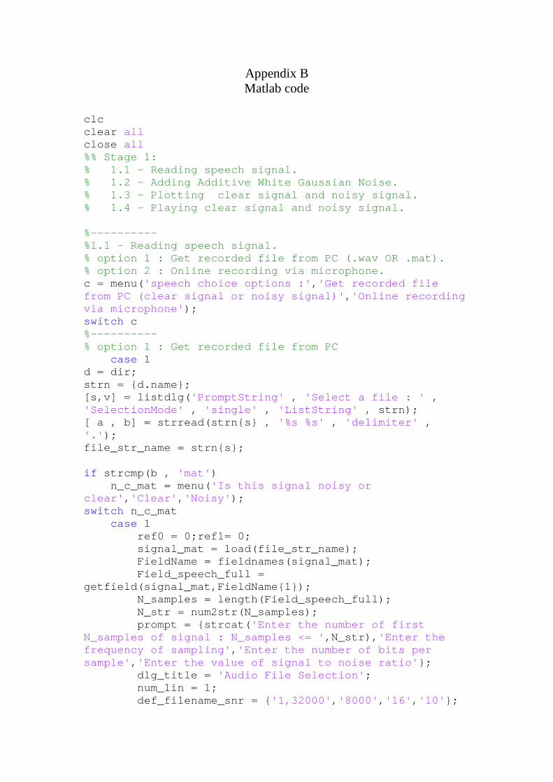
Appendix BMatlab code

clcclear allclose all%% Stage 1:% 1.1 - Reading speech signal.% 1.2 - Adding Additive White Gaussian Noise.% 1.3 - Plotting clear signal and noisy signal.% 1.4 - Playing clear signal and noisy signal.

%----------%1.1 - Reading speech signal.% option 1 : Get recorded file from PC (.wav OR .mat).% option 2 : Online recording via microphone.c = menu('speech choice options :','Get recorded filefrom PC (clear signal or noisy signal)','Online recordingvia microphone');switch c%----------% option 1 : Get recorded file from PC

case 1d = dir;strn = {d.name};[s,v] = listdlg('PromptString' , 'Select a file : ' ,'SelectionMode' , 'single' , 'ListString' , strn);[ a , b] = strread(strn{s} , '%s %s' , 'delimiter' ,'.');file_str_name = strn{s};

if strcmp(b , 'mat')n_c_mat = menu('Is this signal noisy or

clear','Clear','Noisy');switch n_c_mat

case 1ref0 = 0;ref1= 0;signal_mat = load(file_str_name);FieldName = fieldnames(signal_mat);Field_speech_full =

getfield(signal_mat,FieldName{1});N_samples = length(Field_speech_full);N_str = num2str(N_samples);prompt = {strcat('Enter the number of first

N_samples of signal : N_samples <= ',N_str),'Enter thefrequency of sampling','Enter the number of bits persample','Enter the value of signal to noise ratio'};

dlg_title = 'Audio File Selection';num_lin = 1;def_filename_snr = {'1,32000','8000','16','10'};

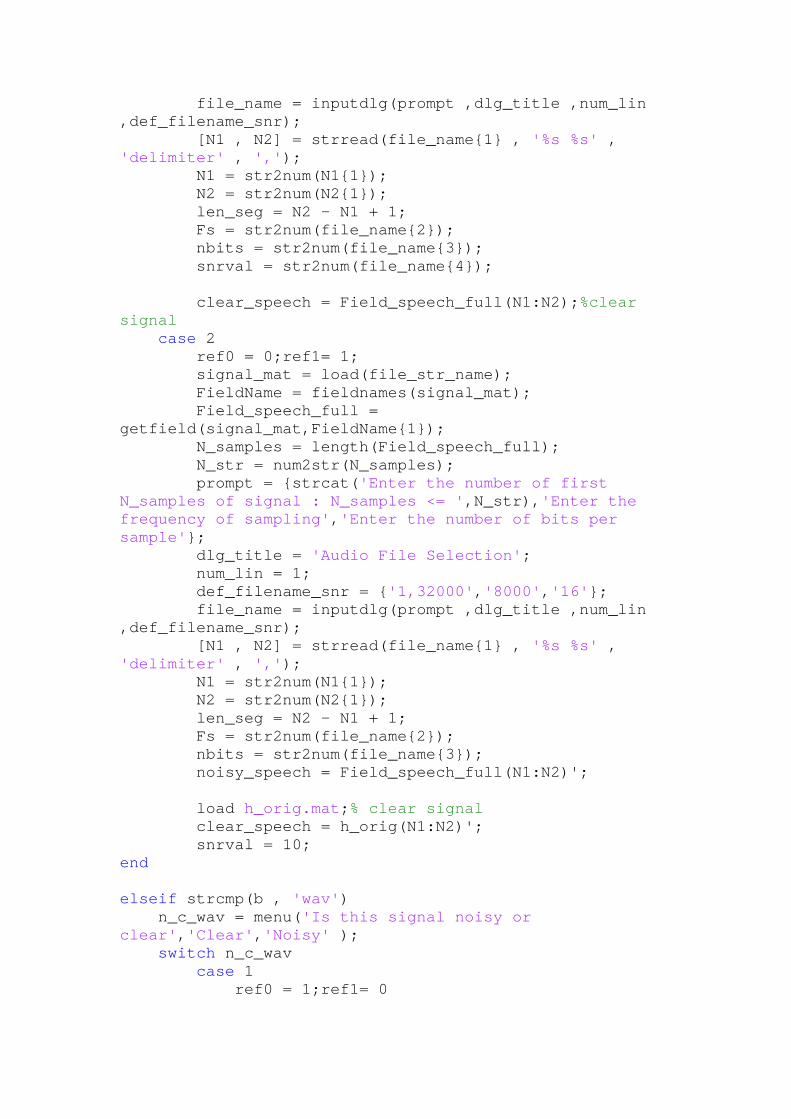
file_name = inputdlg(prompt ,dlg_title ,num_lin,def_filename_snr);

[N1 , N2] = strread(file_name{1} , '%s %s' ,'delimiter' , ',');

N1 = str2num(N1{1});N2 = str2num(N2{1});len_seg = N2 - N1 + 1;Fs = str2num(file_name{2});nbits = str2num(file_name{3});snrval = str2num(file_name{4});

clear_speech = Field_speech_full(N1:N2);%clearsignal

case 2ref0 = 0;ref1= 1;signal_mat = load(file_str_name);FieldName = fieldnames(signal_mat);Field_speech_full =

getfield(signal_mat,FieldName{1});N_samples = length(Field_speech_full);N_str = num2str(N_samples);prompt = {strcat('Enter the number of first

N_samples of signal : N_samples <= ',N_str),'Enter thefrequency of sampling','Enter the number of bits persample'};

dlg_title = 'Audio File Selection';num_lin = 1;def_filename_snr = {'1,32000','8000','16'};file_name = inputdlg(prompt ,dlg_title ,num_lin

,def_filename_snr);[N1 , N2] = strread(file_name{1} , '%s %s' ,

'delimiter' , ',');N1 = str2num(N1{1});N2 = str2num(N2{1});len_seg = N2 - N1 + 1;Fs = str2num(file_name{2});nbits = str2num(file_name{3});noisy_speech = Field_speech_full(N1:N2)';

load h_orig.mat;% clear signalclear_speech = h_orig(N1:N2)';snrval = 10;

end

elseif strcmp(b , 'wav')n_c_wav = menu('Is this signal noisy or

clear','Clear','Noisy' );switch n_c_wav

case 1ref0 = 1;ref1= 0

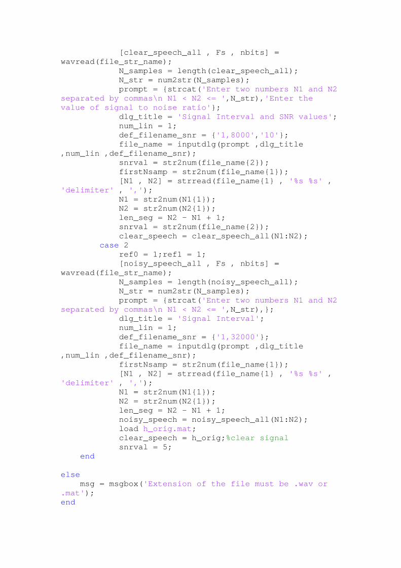
[clear_speech_all , Fs , nbits] =wavread(file_str_name);

N_samples = length(clear_speech_all);N_str = num2str(N_samples);prompt = {strcat('Enter two numbers N1 and N2

separated by commas\n N1 < N2 <= ',N_str),'Enter thevalue of signal to noise ratio'};

dlg_title = 'Signal Interval and SNR values';num_lin = 1;def_filename_snr = {'1,8000','10'};file_name = inputdlg(prompt ,dlg_title

,num_lin ,def_filename_snr);snrval = str2num(file_name{2});firstNsamp = str2num(file_name{1});[N1 , N2] = strread(file_name{1} , '%s %s' ,

'delimiter' , ',');N1 = str2num(N1{1});N2 = str2num(N2{1});len_seg = N2 - N1 + 1;snrval = str2num(file_name{2});clear_speech = clear_speech_all(N1:N2);

case 2ref0 = 1;ref1 = 1;[noisy_speech_all , Fs , nbits] =

wavread(file_str_name);N_samples = length(noisy_speech_all);N_str = num2str(N_samples);prompt = {strcat('Enter two numbers N1 and N2

separated by commas\n N1 < N2 <= ',N_str),};dlg_title = 'Signal Interval';num_lin = 1;def_filename_snr = {'1,32000'};file_name = inputdlg(prompt ,dlg_title

,num_lin ,def_filename_snr);firstNsamp = str2num(file_name{1});[N1 , N2] = strread(file_name{1} , '%s %s' ,

'delimiter' , ',');N1 = str2num(N1{1});N2 = str2num(N2{1});len_seg = N2 - N1 + 1;noisy_speech = noisy_speech_all(N1:N2);load h_orig.mat;clear_speech = h_orig;%clear signalsnrval = 5;

end

elsemsg = msgbox('Extension of the file must be .wav or

.mat');end

if (size(clear_speech,1) == 1)clear_speech = clear_speech';

end

%----------%1.2 - Adding Aditive White Gaussian Noiseif (ref0 == 0 && ref1 == 0) ||(ref0 == 1 && ref1 == 0)noise_generator = menu('noise generator','Add whitegaussian noise to signal' , 'Add normally distributedpseduorandom numbers to signal');if ~(noise_generator-1)noisy_speech = awgn(clear_speech,snrval,'measured');%AddAWGNelsesnr_lin = 10^(snrval/10);power_signal = mean(abs(clear_speech).^2);var = power_signal/snr_lin;noise = (randn(length(clear_speech),1).*sqrt(var));noisy_speech = clear_speech + noise; % Add I.I.D AWGNendend% Test the vector dimensions agreement.

if(size(clear_speech,1)-size(noisy_speech,1))~=0if size(noisy_speech,1)==1

noisy_speech = noisy_speech';else

clear_speech = clear_speech';end

end

save E:\Noisy_File\noisy_speech.matnoisyfile = 'E:\Noisy_File\noisy_speech.wav';wavwrite(noisy_speech, Fs ,nbits, noisyfile)% Write thenoisy signal into noisyfile

%----------%1.3 - Plotting clear signal and noisy signal

%----------fig1 = figure('name' ,'clear and noisy speech

signals','Color','w');%----------

subplot(211); axis tight;plot([1:length(clear_speech)]/Fs , clear_speech ,'b');xlabel('Time(s)'); ylabel('Amplitude');title('Clear speech signal');subplot(212); axis tight;plot([1:length(noisy_speech)]/Fs , noisy_speech,'r');xlabel('Time(s)'); ylabel('Amplitude');

title('Noisy speech signal');%----------%1.4 - Play clean and noisy speech signalPause_t = (length(clear_speech)/Fs) + 2 ;sound(clear_speech,Fs)pause(Pause_t);sound(noisy_speech , Fs)%----------% option 2 : Online recording via microphone

case 2prompt = {'Enter the number of second to be

recorded','Enter the frequency sampling rate'};dlg_title = 'Audio Recording';num_lin = 2;def_t_f = {'5','8000'};record_par = inputdlg(prompt ,dlg_title ,num_lin

,def_t_f);record_t = str2num(record_par{1})Fs = str2num(record_par{2})record_speechObj = audiorecorder(Fs , 16 , 1);msg0 = msgbox('Start speaking');h = waitbar(0,'Start speaking')for step=1:1recordblocking(record_speechObj , record_t);waitbar(step)endmsg1 = msgbox('End speaking');pause(2);close(h)noisy_speech = getaudiodata(record_speechObj ,

'double');

%----------fig2 = figure('name' , 'noisy recorded

speech','Color','w');%----------plot([1:length(noisy_speech)]/Fs ,

noisy_speech);% Plotting the noisy recorded signalplay(record_speechObj); % Play the noisy recorded

speech signalend

%----------

%% Stage 2:% 2.1 - Choose a)DWT or b)DPT% In the case of DWT :% 2.2.a - Set the number of level decomposition and thewavelet function name% 2.3.a - Find the wavelet and scaling functions% 2.4.a - Find the wavelet and scaling filters

% 2.5.a - Decompose the noisy signal at a given levelusing the wavelet filters% 2.6.a - Extract the approximation coefficients atcoarser scale(final level) from% the wavelet decomposition structure [Cad , L]% 2.7.a - Extract the detail coefficients at the levels(1 , 2 , ... , level)% from the wavelet decomposition structure [Cad , L]% 2.8.a - Find the energy of the wavelet coefficients% 2.9.a - Reconstruct the approximation signal atcoarser scale(final level)from wavelet decomposition% 2.10.a - Reconstruct the detail signals at all levelsfrom the wavelet decomposition% structure [Cad , L]% 2.11.a - Plotting illustration

%----------%2.1 - Choose a)DWT or b)DPTc1 = menu('Denoising using :' ,'Discrete WaveletTransform (DWT)','Discrete Wavelet packet (DWP)');switch c1

case 1% DWT%----------%2.2.a - Set the number of level decomposition and thewavelet function namelev_wname = inputdlg({'Enter the number of decompositionlevels','Enter the wave name : dbN'},'Number of level andwavename');level = str2num(lev_wname{1});wavename = lev_wname{2};%----------%2.3.a - Find the wavelet and scaling functionsiteration = 15;[phi , psi , xval_dbn] = wavefun(wavename , iteration);%----------%2.4.a - Find the wavelet and scaling filters[Lo_d , Lo_r] = wfilters(wavename , 'l')Hi_r = qmf(Lo_r)Hi_d = wrev(Hi_r)

sum_Hi_d = sum(Hi_d)sum_Lo_d = sum(Lo_d)

Nextpow2_Lo_d = nextpow2(length(Lo_d));Nextpow2_Hi_d = nextpow2(length(Lo_d));Nextpow2_Lo_r = nextpow2(length(Lo_r));Nextpow2_Hi_r = nextpow2(length(Lo_r));

fftLo_d = fft(Lo_d,2^Nextpow2_Lo_d);fftHi_d= fft(Hi_d,2^Nextpow2_Hi_d);fftLo_r = fft(Lo_r,2^Nextpow2_Lo_r);

fftHi_r= fft(Hi_r,2^Nextpow2_Hi_r);

%----------%2.5.a - Decompose the noisy signal at a given levelusing the wavelet filters[Cad , L] = wavedec(noisy_speech(:,1) ,level , wavename);%----------%2.6.a - Extract the approximation coefficients%2.7.a - Extract the detail coefficients%2.8.a - Find the energy of the wavelet coefficientsCapp = appcoef(Cad , L , Lo_d , Hi_d, level);%Extract theapproximation coefficients for level (level)a2sq = sum(Capp.^2);%energy of the wavelet approximationcoefficientsEnergy_coef = zeros(1,level+1);Energy_coef(1) = a2sq;SDEV = zeros(1,level);SDEV_COEF = zeros(1,level);for i= level : -1 : 1

Cdet = detcoef(Cad , L , i);% Extract the detailcoefficients for level (i)

d2sq = sum(Cdet.^2);Array_det_coef{level-i+1} = Cdet;d2sq = sum(Array_det_coef{level-i+1}.^2);%energy of

the wavelet coefficients for every scaleEnergy_coef(level-i+2)= d2sq;SDEV(i) = wnoisest(Cad , L ,i);% standard deviation

appriximation for detail coefficients for every scaleSDEV_COEF(i) = std(Cdet);

endengcoef = sum(Energy_coef)% total energy of waveletcoefficients(approximation & detail)engsig = sum(noisy_speech(:,1).^2)% total energy of thenoisy signalengerr = abs(engcoef - engsig)% energy preservationpercent_energy_app =(Energy_coef(1)/sum(Energy_coef))*100%----------%2.9.a - Reconstruct the approximation signal at coarserscale(final level)from wavelet decompositionApp_sig = wrcoef('a' , Cad , L , wavename , level);ReconstructArray_sig{1} = App_sig;%----------%2.10.a - Reconstruct the detail signals at all levelsfrom the wavelet decompositionSDEV_REC = zeros(1,level);for j = level : -1 : 1

Det_sig = wrcoef('d' , Cad , L , wavename , j);ReconstructArray_sig{level-j+2} = Det_sig;SDEV_REC(j) = std(Det_sig);

end

%----------%2.11.a - Plotting illustration

%----------fig3 = figure('name' , 'phi_psi functions ,filters

and fft of filters','Color','w');%----------

subplot(521); axis tight ;plot(xval_dbn, phi);title('Scaling function phi');subplot(522); axis tight ;plot(xval_dbn, psi);title('Wavelet function psi');

subplot(523); axis tight ;stem(Lo_d,'r');title('Decomposition low pass filter');subplot(524); axis tight ;stem(Hi_d,'r');title('Decomposition high pass filter');subplot(525); axis tight ;stem(Lo_r,'b');title('Reconstruction low pass filter');subplot(526); axis tight ;stem(Hi_r,'b');title('Reconstruction high pass filter');

subplot(527); axis tightFreq_Lo_d = (2*pi)/(2^Nextpow2_Lo_d):(2*pi)/(2^Nextpow2_Lo_d) : pi ;fa_ld = abs(fftLo_d(1:(2^(Nextpow2_Lo_d)/2)));plot(Freq_Lo_d,fa_ld);title('FFT of analysis low passfilter');xlim([(2*pi)/(2^Nextpow2_Lo_d) , pi+0.5]);

subplot(528); axis tightFreq_Lo_r = (2*pi)/(2^Nextpow2_Lo_r):(2*pi)/(2^Nextpow2_Lo_r) : pi ;fa_hr = abs(fftLo_r(1:(2^(Nextpow2_Lo_r)/2)));plot(Freq_Lo_r,fa_hr);title('FFT of synthesis low passfilter');xlim([(2*pi)/(2^Nextpow2_Lo_r) , pi+0.5]);

subplot(529); axis tightFreq_Hi_d = (2*pi)/(2^Nextpow2_Hi_d):(2*pi)/(2^Nextpow2_Hi_d) : pi ;fa_ld = abs(fftHi_d(1:((2^Nextpow2_Hi_d)/2)));plot(Freq_Hi_d,fa_ld);title('FFT of analysis high passfilter');xlim([(2*pi)/(2^Nextpow2_Hi_d) , pi+0.5]);

subplot(5,2,10); axis tightFreq_Hi_r = (2*pi)/(2^Nextpow2_Hi_r):(2*pi)/(2^Nextpow2_Hi_r) : pi ;fa_hr = abs(fftHi_r(1:((2^Nextpow2_Hi_r)/2)));

plot(Freq_Hi_r,fa_hr);title('FFT of synthesis high passfilter');xlim([(2*pi)/(2^Nextpow2_Hi_r) , pi+0.5]);

%----------fig4 = figure('name' , 'decomposition

coefficients','Color','w');%----------

subplot(level+2,1,1); axis tight;plot([1:length(noisy_speech)]/Fs , noisy_speech,'r');title('Noisy speech signal');subplot(level+2,1,2); axis tight;plot(Capp , 'b')title(['Approximation coefficients at level ',num2str(level)]);ylabel(['Ca' , num2str(level)], 'Color' , 'b');for f = level : -1 : 1

row = level+2;no_fig = level-f+3;s = level-f+1;lbl = num2str(f);

subplot(row,1,no_fig); axis tight;plot(Array_det_coef{s} , 'g')title(['Detail coefficients at level ' ,lbl]);ylabel(['Cd',lbl],'Color' , 'g')endsubplot(row,1,row)

%----------fig5 = figure('name' , 'reconstructed

coefficients','Color','w') ;%----------

subplot(level+2,1,1); axis tight;plot([1:length(noisy_speech)]/Fs , noisy_speech,'r');title(['Noisy speech signal : a',num2str(level),' +d',num2str(level),' = d',num2str(level-1)]);subplot(level+2,1,2); axis tight;plot( ReconstructArray_sig{1} , 'b')title(['Approximation signal at level ',num2str(level)]);ylabel(['a' ,num2str(level)],'Color' , 'b')for r = level : -1 : 1

row = level+2;no_fig = level-r+3;s = level-r+1;lbl = num2str(r);

subplot(row,1,no_fig); axis tight;plot(ReconstructArray_sig{level-r+2} , 'g')

title(['Reconstructed coefficients at level ' ,lbl]);ylabel(['d' , lbl],'Color' , 'g')endsubplot(row,1,row);xlabel('Time');

%----------fig6 = figure('name' , 'energy and standard

deviation','Color','w');%----------

subplot(211) , axis tight;stem(Energy_coef(2:end),'g');hold onstem(Energy_coef(1),'b');title('Energy of coefficients at different scale');xlabel('level number'); ylabel('energy of coefficients');legend('detail coefficients energy','approximationcoefficients energy')subplot(212); axis tight;stem(wrev(SDEV.^2),'r'); title('Variance of details atdifferent scales');xlabel('level number'); ylabel('Variance of details atdifferent scales');

tilefigs%----------

%% Stage 3:% 3.1.a - Choose the type of thresholding function (soft or hard)% s : soft thresholding or h : hardthresholding% 3.2.a - Decide whether you need to threshod theapproximation coefficient or not% KeepApp = 1 : withno threshold approx.coeff's or KeepApp = 0 : with threshold approx. coeff's% 3.3.a - Set the value of threshold (this value forglobal thresholding)% The above three steps could also be choosen bydefault option instead of manual option.% 3.4.a - Choose the type of thresholding% 3.4.a.1 - gbl : global thresholding% 3.4.a.2 - lvd : level dependent thresholding% 3.4.a.2.1 - Choose the noise model% 3.4.a.2.2 - Chooose the thresholdselection rule% 3.4.a.2.3 - Calculate the thresholdvector which contains% the threshold values forevery level

% 3.4.a.3 selected level thresholding% 3.4.a.3.1 - Choose selcted levelthresholding methology% ( set all coeff's of selected level tozero or threshod the selected level by (s or h) )% 3.4.a.3.2 - Decide the level numbers tobe thresholded% 3.4.a.4 Interval dependent thresholding% 4.4.a - Reconstruct the signal from thresholdedcoefficients% 4.5.a - Reconstruct the approximation and detailsignals from wavelet thresholded decomposition% 4.6.a - Plotting illustration% 4.7.a - Playing the denoised speech

%----------%3.1.a - Choose the type of thresholding function ( softor hard)%3.2.a - Decide whether you need to threshod theapproximation coefficient or not%3.3.a - Set the value of threshold (this value forglobal thresholding)%The above three steps could also be choosen by defaultoption instead of manual option.setting = menu('Set the values of (threshold value , softor hard thresholding function , KeepApp)','manualsetting','defult setting');switch setting

case 1std_glb =

median(abs(Array_det_coef{level}))/0.6745;thr = std_glb*sqrt(2*log(length(noisy_speech)));thr_globstr = num2str(thr);def_thr_s_1 = {thr_globstr,'s','1'};thr_sorh_k = inputdlg({'Enter the value of

threshold','Enter the type of thresholding function softor hard s or h','Threshold the approximation? 1:no or0:yes'},'Setting parameters',1,def_thr_s_1);

thr = str2num(thr_sorh_k{1});s_or_h = thr_sorh_k{2};KeepApp = str2num(thr_sorh_k{3});

case 2% the default value of the threshold is

calculated as thr = std*sqrt(2*log(length(noisy_speech)))where std = median(abs(D))/0.6745

% such that D is calculated form the single levelDWT using haar wavelet.[D , A] = dwt('db1' ,noisy_speech];also, std(noise) = median(abs(D))/0.6745

[thr , s_or_h , KeepApp] = ddencmp('den' , 'wv' ,noisy_speech(:,1));

default_dialog = msgbox({'thr = ',num2str(thr),'s_or_h = ' ,s_or_h, 'Keepapp =',num2str(KeepApp)},'Default values');end%----------%3.4.a - Choose the type of thresholding

gbl_or_lvd = menu('Type of thresholding','Globalthresholding','Level-dependent thresholding','1-D waveletcoefficients thresholding','Interval-dependentthresholding');msg2 = msgbox('De_noising ...');

FrameSelection = menu('Do you want to segment the speechor not?','Yes','No');

switch FrameSelectioncase 1

seg_step = Fs*0.01;overlap = Fs*0.01;seg_len = seg_step + overlap;sp_len = length(noisy_speech);Nseg = floor(sp_len/(seg_step))-1;window = hamming(seg_len);de = hanning(2*overlap - 1)';dewindow = [de(1:overlap) , ones(1,seg_len -2*overlap) ,de(overlap:end)]'./window;

switch gbl_or_lvd%----------%3.4.a.1 - gbl : global thresholdingcase 1

%----------%4.4.a - Reconstruct the signal from thresholdedcoefficients

denoised_speech = zeros(sp_len, 1);

for i = 1 : Nsegsp_Seg(:,i) = noisy_speech((i-1)*seg_step+1 :

i*seg_step+overlap);

noisy_speechW(:,i) = window.*sp_Seg(:,i);[Cad_seg , L] =

wavedec(noisy_speechW(:,i),level,wavename);

Cdet_seg = detcoef(Cad_seg , L , 1);sigma_seg = median(abs(Cdet_seg))/0.6745;thr_seg =

sigma_seg*sqrt(2*log(length(noisy_speechW(:,i))));

[denoised_seg ,Cad_thr_seg , L_thr_seg ,L2norm_recovery_seg , cmp_score_seg] = wdencmp('gbl' ,Cad_seg , L , wavename , level ,thr_seg , s_or_h , 1);

denoised_seg (:,i) = denoised_seg;noisy_speechDe(:,i) = denoised_seg (:,i).*dewindow;denoised_speech((i-1)*seg_step+1 :

i*seg_step+overlap) = noisy_speechDe(:,i) +denoised_speech((i-1)*seg_step+1 : i*seg_step+overlap);end%----------

%----------%3.4.a.2 - lvd : level-dependent thresholdingcase 2

THR_setManual = menu('Choose the thresholds (onlydetails coefficients) for level-dependetthresholding','Manual setting','Based on thresholdselection rules');

if ~(THR_setManual-1)THR_dlg = inputdlg({'Enter a list of thresholds

seperated by commas'},'Thresholds setting for level-dependent')

THR = str2num(THR_dlg{1});

else

%----------%3.4.a.2.1 - Choose the noise modelnoise_mod_menu = menu('Noise model','Unscaled

white noise','Scaled white noise','Non-white noise');noise_model = {'one' , 'sln' , 'mln'};SCAL = noise_model(noise_mod_menu);f =char(SCAL{1})%----------%3.4.a.2.2 - Chooose the threshold selection rulethrrule = menu('Threshold selection

rule','rigrsure' ,'heursure' , 'sqtwolog' , 'minimaxi');menu_thrrule = {'rigrsure' ,'heursure' ,

'sqtwolog' , 'minimaxi'};ThrSelectRule = menu_thrrule(thrrule);tptr = ThrSelectRule{1}%----------denoised_speech = zeros(sp_len , 1);

for i = 1 : Nsegsp_Seg(:,i) = noisy_speech((i-1)*seg_step+1 :

i*seg_step+overlap);noisy_speechW(:,i) = window.*sp_Seg(:,i);

denoised_seg =wden(noisy_speechW(:,i),tptr,s_or_h,f,level,wavename);

denoised_seg(:,i) = denoised_seg;noisy_speechDe(:,i) = denoised_seg (:,i).*dewindow;denoised_speech((i-1)*seg_step+1 :

i*seg_step+overlap) = noisy_speechDe(:,i) +denoised_speech((i-1)*seg_step+1 : i*seg_step+overlap);

THR = zeros(1,level);end

end%----------

%----------

%----------%3.4.a.3 selected level thresholding (only details

coefficients)case 3

%----------%3.4.a.3.1 - Choose selcted level thresholding

methologyx = menu('detail coeficients

thresholding:','thresholding the details for a given setof level by forceing all coefficients to bezero','thresholding the details for a given set of levelby using soft or hard thresholding function');

if ~(x-1) %set all coeff's of selected level tozero

selected_lev = inputdlg({'Enter a list ofnumbers (number of levels for thresholding)separated byspaces or commas'},'Wavelet coefficient thresholding');

LEV = str2num(selected_lev{1});

denoised_speech = zeros(sp_len,1);

for i = 1 : Nsegsp_Seg(:,i) = noisy_speech((i-1)*seg_step+1 :

i*seg_step+overlap);

noisy_speechW(:,i) = window.*sp_Seg(:,i);

[Cad_seg , L] =wavedec(noisy_speechW(:,i),level,wavename);

Cdet_seg = detcoef(Cad_seg , L , 1);Capp = appcoef(Cad_seg,L,wavename,1);sigma_seg = median(abs(Cdet_seg))/0.6745;thr_seg = sigma_seg*sqrt(2*log(length(sp_Seg(:,i))));

Cad_thr_seg = wthcoef('d' , Cad_seg , L , 1);denoised_seg = waverec(Cad_thr_seg,L,wavename);

denoised_seg(:,i) = denoised_seg;noisy_speechDe(:,i) = denoised_seg (:,i).*dewindow;denoised_speech((i-1)*seg_step+1 :

i*seg_step+overlap) = noisy_speechDe(:,i) +denoised_speech((i-1)*seg_step+1 : i*seg_step+overlap);end

else %threshod the selected level by (s or h)

selected_lev = inputdlg({'Enter a list ofnumbers (number of levels for thresholding)separated byspaces or commas','Enter the crrespondingthresholds'},'Wavelet coefficient thresholding');

LEV = str2num(selected_lev{1});T = str2num(selected_lev{2});

denoised_speech = zeros(sp_len,1);

for i = 1 : Nsegsp_Seg(:,i) = noisy_speech((i-1)*seg_step+1 :

i*seg_step+overlap);

noisy_speechW(:,i) = window.*sp_Seg(:,i);

[Cad_seg , L] =wavedec(noisy_speechW(:,i),level,wavename);

Cdet_seg = detcoef(Cad_seg , L , 1);Capp = appcoef(Cad_seg,L,wavename,1);sigma_seg = median(abs(Cdet_seg))/0.6745;thr_seg = sigma_seg*sqrt(2*log(length(sp_Seg(:,i))));

Cad_thr_seg = wthcoef('t' , Cad_seg , L , LEV,T,s_or_h);

denoised_seg = waverec(Cad_thr_seg,L,wavename);

denoised_seg(:,i) = denoised_seg;noisy_speechDe(:,i) = denoised_seg (:,i).*dewindow;denoised_speech((i-1)*seg_step+1 :

i*seg_step+overlap) = noisy_speechDe(:,i) +denoised_speech((i-1)*seg_step+1 : i*seg_step+overlap);end

end%----------

%----------%3.4.a.4 - Interval-dependent thresholdingcase 4

x1 = menu('Interval-dependentdenoising:','Interval-dependent denoising based onvariance change');

num_int = inputdlg({'Enter the number ofintervals'} ,'Number of intervals' , 1 ,{'1'});

nb_int = str2num(num_int{1});denoised_speech = zeros(sp_len,1);

for i = 1 : Nsegsp_Seg(:,i) = noisy_speech((i-1)*seg_step+1 :

i*seg_step+overlap);

noisy_speechW(:,i) = window.*sp_Seg(:,i);

[denoised_seg,Cad_thr_seg,thrParamsOut_seg,int_DepThr_Cell_seg,BestNbOfInt_seg] =cmddenoise(noisy_speechW(:,i),wavename,level,s_or_h,nb_int);

denoised_seg = denoised_seg';denoised_seg0(:,i) = denoised_seg;noisy_speechDe(:,i) = denoised_seg0(:,i).*dewindow;denoised_speech((i-1)*seg_step+1 :

i*seg_step+overlap) = noisy_speechDe(:,i) +denoised_speech((i-1)*seg_step+1 : i*seg_step+overlap);end

%

end

[Cad_thr , L] =wavedec(denoised_speech,level,wavename);

case 2

switch gbl_or_lvd%----------%3.4.a.1 - gbl : global thresholdingcase 1

%----------%4.4.a - Reconstruct the signal from thresholdedcoefficients

[denoised_speech ,Cad_thr , L_thr ,L2norm_recovery , cmp_score] = wdencmp('gbl' , Cad , L ,wavename , level,thr , s_or_h , KeepApp);

L2norm_recovery ,cmp_score%----------

%----------%3.4.a.2 - lvd : level-dependent thresholding

case 2THR_setManual = menu('Choose the thresholds (only

details coefficients) for level-dependetthresholding','Manual setting','Based on thresholdselection rules');

if ~(THR_setManual-1)THR_dlg = inputdlg({'Enter a list of thresholds

seperated by commas'},'Thresholds setting for level-dependent')

THR = str2num(THR_dlg{1});

else

%----------%3.4.a.2.1 - Choose the noise modelnoise_mod_menu = menu('Noise model','Unscaled

white noise','Scaled white noise','Non-white noise');noise_model = {'one' , 'sln' , 'mln'};SCAL = noise_model(noise_mod_menu);f =char(SCAL{1})%----------%3.4.a.2.2 - Chooose the threshold selection rulethrrule = menu('Threshold selection

rule','rigrsure' ,'heursure' , 'sqtwolog' , 'minimaxi');%----------%3.4.a.2.3 - Calculate the threshold vectorswitch thrrule

case 1THR= wthrmngr('dw1ddenoLVL' ,'rigrsure',Cad , L

,f);case 2

THR= wthrmngr('dw1ddenoLVL' ,'heursure',Cad , L,f);

case 3THR= wthrmngr('dw1ddenoLVL','sqtwolog',Cad , L

,f);case 4

THR= wthrmngr('dw1ddenoLVL' ,'minimaxi',Cad , L,f);

end%----------end

%----------

%----------%4.4.a - Reconstruct the signal from the thresholdedcoefficients

[denoised_speech ,Cad_thr , L_thr ,L2norm_recovery , cmp_score] = wdencmp('lvd' , Cad , L ,wavename ,level , THR , s_or_h);

%----------

%----------%3.4.a.3 selected level thresholding (only details

coefficients)case 3

%----------%3.4.a.3.1 - Choose selcted level thresholding

methologyx = menu('detail coeficients

thresholding:','thresholding the details for a given setof level by forceing all coefficients to bezero','thresholding the details for a given set of levelby using soft or hard thresholding function');

if ~(x-1) %set all coeff's of selected level tozero

selected_lev = inputdlg({'Enter a list ofnumbers (number of levels for thresholding)separated byspaces or commas'},'Wavelet coefficient thresholding');

LEV = str2num(selected_lev{1});Cad_thr = wthcoef('d' , Cad , L , LEV);%1<=

N(i)<=length(L)-2else %threshod the selected level by (s or h)

selected_lev = inputdlg({'Enter a list ofnumbers (number of levels for thresholding)separated byspaces or commas','Enter the crrespondingthresholds'},'Wavelet coefficient thresholding');

LEV = str2num(selected_lev{1});T = str2num(selected_lev{2});

Cad_thr = wthcoef('t' , Cad , L , LEV ,T,s_or_h);end%----------

%----------

%----------%4.4.a - Reconstruct the signal from the thresholdedcoefficients

denoised_speech = waverec(Cad_thr,L,wavename);%----------

%----------%3.4.a.4 - Interval-dependent thresholdingcase 4

x1 = menu('Interval-dependentdenoising:','Interval-dependent denoising based onvariance change','Manual setting for intervals and itsthresholds');

if ~(x1-1)num_int = inputdlg({'Enter the number of

intervals'} ,'Number of intervals' , 1 ,{'1'});

nb_int = str2num(num_int{1});

[denoised_speech,Cad_thr,thrParamsOut,int_DepThr_Cell,BestNbOfInt] =cmddenoise(noisy_speech,wavename,level,s_or_h,nb_int);

denoised_speech = denoised_speech';

elsecel = cell(1,level);def = cell(1,level);for w0 = 1 :level

cel{w0} = strcat('level',' ',num2str(w0));

def{w0} = strcat('start , end , thr ;...');

endoptions.Resize = 'on';THR_int_dep = inputdlg(cel,'Threshold setting

for interval-dependent thresholding',level,def,options);for w1 = 1:levelf = str2num(THR_int_dep{w1});cel{w1} = f;endCad_thr =

cadthrCompute(cel,Cad,L,level,s_or_h);

denoised_speech =cmddenoise(noisy_speech,wavename,level,s_or_h,NaN,cel);

denoised_speech = denoised_speech';end

%----------%4.5.a - Reconstruct the approximation and detail signalsfrom wavelet thresholded decomposition

App_den_sig = wrcoef('a', Cad_thr , L ,wavename , level);

ReconstructArray_densig{1} = App_den_sig;for k0 = level : -1 : 1

Det_den_sig = wrcoef('d' , Cad_thr , L ,wavename , k0);

ReconstructArray_densig{k0+1} =Det_den_sig;

endendend

case 2 %DWP%----------

%2.2.a - Set the number of level decomposition and thewavelet function name

lev_wname = inputdlg({'Enter the number of decompositionlevels','Enter the wave name : dbN'},'Number of level andwavename');level = str2num(lev_wname{1});wavename = lev_wname{2};%----------%2.3.a - Find the wavelet and scaling functions[W , xval_dbn] = wpfun(wavename ,7);%----------%2.4.a - Find the wavelet and scaling filters[Lo_d , Lo_r] = wfilters(wavename , 'l')Hi_r = qmf(Lo_r)Hi_d = wrev(Hi_r)

sum_Hi_d = sum(Hi_d);sum_Lo_d = sum(Lo_d);

Nextpow2_Lo_d = nextpow2(length(Lo_d));Nextpow2_Hi_d = nextpow2(length(Lo_d));Nextpow2_Lo_r = nextpow2(length(Lo_r));Nextpow2_Hi_r = nextpow2(length(Lo_r));

fftLo_d = fft(Lo_d,2^Nextpow2_Lo_d);fftHi_d= fft(Hi_d,2^Nextpow2_Hi_d);fftLo_r = fft(Lo_r,2^Nextpow2_Lo_r);fftHi_r= fft(Hi_r,2^Nextpow2_Hi_r);%----------%2.5.a - Decompose the noisy signal at a given levelusing the wavelet filterswpt = wpdec(noisy_speech ,level , wavename);%----------cfs_cell = cell(1,level);rcfs_cell = cell(1,level);for i = 1 :level+1

for j = 0 : (2^level)-1node(1) = i-1;node(2) = j;

cfs_cell{i} = wpcoef(wpt,[node(1),node(2)]);rcfs_cell{i} = wprcoef(wpt,[node(1),node(2)]);

endend%----------det_first_scl = wpcoef(wpt,[1 1]);sigma_stdNoise = median(det_first_scl)/0.6745;alpha = 2thr = wpbmpen(wpt,sigma_stdNoise,alpha);setting = menu('Set the values of (threshold value , softor hard thresholding function , KeepApp)','setting');

thr_str = num2str(thr);def_thr_s_1 = {thr_str,'s','1'};

thr_sorh_k = inputdlg({'Enter the value ofthreshold','Enter the type of thresholding function softor hard s or h','threshold the approximation 1 or0'},'Setting parameters',1,def_thr_s_1);

thr = str2num(thr_sorh_k{1});s_or_h = thr_sorh_k{2};KeepApp = str2num(thr_sorh_k{3});

NT = wpthcoef(wpt,KeepApp,s_or_h,thr);denoised_speech = wprec(NT);

%denoised_speech =wpdencmp(wpt,s_or_h,'nobest',thr,KeepApp);%----------

%----------fig7 = figure('name' , strcat('The ',wavename,'

Wavelet Packets'),'Color','w');%----------

[ d_str , moment_str] = strread(wavename , '%s %s' ,'delimiter' , 'b');

moment = str2num(moment_str{1});for wfun=1:8

subplot(2,4,wfun); axis tight;plot(xval_dbn,W(wfun,:));xlabel(strcat('W',num2str(wfun-1)));xlim([0,(2*moment)-1]);

endtitle(strcat('The ',wavename,' Wavelet Packets'));

%----------fig8 = figure('name' , 'filters and fft of

filters','Color','w');%----------

subplot(421); axis tight ;stem(Lo_d,'r');title('Decomposition low pass filter');subplot(422); axis tight ;stem(Hi_d,'r');title('Decomposition high pass filter');subplot(423); axis tight ;stem(Lo_r,'b');title('Reconstruction low pass filter');subplot(424); axis tight ;stem(Hi_r,'b');title('Reconstruction high pass filter');

subplot(425); axis tightFreq_Lo_d = (2*pi)/(2^Nextpow2_Lo_d):(2*pi)/(2^Nextpow2_Lo_d) : pi ;fa_ld = abs(fftLo_d(1:(2^(Nextpow2_Lo_d)/2)));plot(Freq_Lo_d,fa_ld);title('FFT of analysis low passfilter');xlim([(2*pi)/(2^Nextpow2_Lo_d) , pi+0.5]);

subplot(426); axis tightFreq_Lo_r = (2*pi)/(2^Nextpow2_Lo_r):(2*pi)/(2^Nextpow2_Lo_r) : pi ;fa_hr = abs(fftLo_r(1:(2^(Nextpow2_Lo_r)/2)));plot(Freq_Lo_r,fa_hr);title('FFT of synthesis low passfilter');xlim([(2*pi)/(2^Nextpow2_Lo_r) , pi+0.5]);

subplot(427); axis tightFreq_Hi_d = (2*pi)/(2^Nextpow2_Hi_d):(2*pi)/(2^Nextpow2_Hi_d) : pi ;fa_ld = abs(fftHi_d(1:((2^Nextpow2_Hi_d)/2)));plot(Freq_Hi_d,fa_ld);title('FFT of analysis high passfilter');xlim([(2*pi)/(2^Nextpow2_Hi_d) , pi+0.5]);

subplot(428); axis tightFreq_Hi_r = (2*pi)/(2^Nextpow2_Hi_r):(2*pi)/(2^Nextpow2_Hi_r) : pi ;fa_hr = abs(fftHi_r(1:((2^Nextpow2_Hi_r)/2)));plot(Freq_Hi_r,fa_hr);title('FFT of synthesis high passfilter');xlim([(2*pi)/(2^Nextpow2_Hi_r) , pi+0.5]);end

%----------%4.6.a/b - Plotting illustration

%----------fig9 = figure('name' , 'thresholding function

illustration','Color','w');%----------

lin_fun = linspace(-0.5 , 0.5 , 100);lin_fun_s = wthresh(lin_fun , 's' , thr);lin_fun_h = wthresh(lin_fun , 'h' , thr);subplot(131); plot(lin_fun,lin_fun,'k'); title('Originalfunction');subplot(132); plot(lin_fun,lin_fun_s,'b'); title('Softthresholded function');text(thr , -0.05 , [ strcat('(',num2str(thr),',') ,strcat(num2str(0),')')],'Color' ,'b','HorizontalAlignment','center')subplot(133); plot(lin_fun,lin_fun_h,'r'); title('Hardthresholded function');text(thr , -0.05 , [ strcat('(',num2str(thr),',') ,strcat(num2str(0),')')],'Color' ,'r','HorizontalAlignment','center')for fig = 1 : 3

subplot(1,3,fig)xlabel('coefficients before thresholding');

ylabel('coefficients after thresholding');endshg

switch ccase 1

%----------fig10 = figure('name' , 'clear , Noisy and Denoised

speech signals','Color','w');%----------

subplot(2,4,1:2); axis tight;plot([1:length(noisy_speech)]/Fs , noisy_speech ,'r');xlabel('Time(s)'); ylabel('Amplitude');title('Noisy speech signal');

subplot(2,4,3:4); axis tight;plot([1:length(denoised_speech)]/Fs ,denoised_speech,'k');xlabel('Time(s)'); ylabel('Amplitude');title('De-noised speech signal');

subplot(2,4,6:7); axis tight;residual = denoised_speech - clear_speech;plot([1:length(denoised_speech)]/Fs , residual,'g');xlabel('Time(s)'); ylabel('Amplitude');title('Residual signal');

%----------fig11 = figure('name' , 'clear , Noisy and Denoised

speech signals','Color','w');%----------

subplot(211); axis tight;plot([1:length(clear_speech)]/Fs , clear_speech ,'b');xlabel('Time(s)'); ylabel('Amplitude');title('Clear and denoised speech signals');hold on;plot([1:length(denoised_speech)]/Fs ,denoised_speech,'k');legend('clear speech' , 'denoised speech');

subplot(212); axis tight;plot([1:length(noisy_speech)]/Fs , noisy_speech ,'r');xlabel('Time(s)'); ylabel('Amplitude');title('noisy and denoised speech signals');hold on;plot([1:length(denoised_speech)]/Fs ,denoised_speech,'k');legend('noisy speech' , 'denoised speech');

%----------fig12 = figure('name' , 'correlation','Color','w');%----------

subplot(211); axis tight;[xcor_bef , lag_bef] = crosscorr(clear_speech ,noisy_speech);xc_bef = xcor_bef(21);plot(lag_bef , xcor_bef);xlabel('lag'); ylabel('sample cross correlation');title('correlation between clear signl and noisysignal');

subplot(212); axis tight;[xcor_aft,lag_aft] = crosscorr(clear_speech ,denoised_speech);xc_aft = xcor_aft(21);plot(lag_aft , xcor_aft);xlabel('lag'); ylabel('sample cross correlation');title('correlation between clear signl and denoisedsignal');

%----------fig13 = figure('name' , 'power

distribution','Color','w');%----------

Npow2 = pow2(nextpow2(length(denoised_speech)));denoised_speech_pad = fft(denoised_speech , Npow2);noisy_speech_pad = fft(noisy_speech , Npow2);clear_speech_pad = fft(clear_speech , Npow2);

freq_range = (0:(Npow2 - 1))*(Fs/Npow2);

power_denoised_speech =denoised_speech_pad.*conj(denoised_speech_pad)/Npow2;power_noisy_speech =noisy_speech_pad.*conj(noisy_speech_pad)/Npow2;power_clear_speech =clear_speech_pad.*conj(clear_speech_pad)/Npow2;

subplot(131); axis tight;plot(freq_range , power_denoised_speech);xlabel('frequency Hz'); ylabel('power');title('power distribution of denoised speech signal');

subplot(132); axis tight;plot(freq_range , power_noisy_speech);xlabel('frequency Hz'); ylabel('power');title('power distribution of noisy speech signal');

subplot(133); axis tight;plot(freq_range , power_clear_speech);xlabel('frequency Hz'); ylabel('power');title('power distribution of clear speech signal');

%----------fig14 = figure('name' , 'Spectrograms','Color','w');%----------

subplot(131);spectrogram(clear_speech);ylabel('Time(ms)');title('Spectrogram of clear speech')subplot(132);spectrogram(noisy_speech);ylabel('Time(ms)');title('Spectrogram of noisy speech')subplot(133);spectrogram(denoised_speech);ylabel('Time(ms)');title('Spectrogram of denoised speech')figx = figure('name' , 'Spectrograms of noisy anddenoised speech signals','Color','w');subplot(311);plot([1:length(noisy_speech)]/Fs , noisy_speech ,'r');xlabel('Time(s)'); ylabel('Amplitude');title('noisy and denoised speech signals');hold on;plot([1:length(noisy_speech)]/Fs , denoised_speech,'k');subplot(312);spectrogram(noisy_speech,'yaxis');xlabel('Time(ms)')title('Spectrogram of noisy speech signal')subplot(313);spectrogram(denoised_speech,'yaxis');xlabel('Time(ms)')title('Spectrogram of de-noised speech signal')

if(c1-1)

%----------fig15 = figure('name','Wavelet Packet

Spectrum','Color','w');%----------

subplot(131);[spect_noisy_coef,Time0,Frequency0] =wpspectrum(wpt,Fs,'plot');title('Wavelet Packet Decomposition of Noisy Speech')subplot(132);[spect_denoised_coef,Time1,Frequency1] =wpspectrum(NT,Fs,'plot');title('Wavelet Packet Decomposition of Denoised Speech')subplot(133);

wpt_c = wpdec(clear_speech ,level , wavename);[spect_clear_coef,Time2,Frequency2] =wpspectrum(wpt_c,Fs,'plot');title('Wavelet Packet Decomposition of Clear Speech')else

%----------fig15 = figure('name' , 'Absolute coefficients of

DWT','Color','w');%----------

[Cad_clear , L] = wavedec(clear_speech,level,wavename);

len = length(clear_speech);cfd1 = zeros(level,len);cfd2 = zeros(level,len);cfd3 = zeros(level,len);for k0 = 1 : level

d_1 = detcoef(Cad_clear,L,k0);d_2 = detcoef(Cad,L,k0);d_3 = detcoef(Cad_thr,L,k0);d_1 = d_1(:)';d_2 = d_2(:)';d_3 = d_3(:)';d_1 = d_1(ones(1,2^k0),:);d_2 = d_2(ones(1,2^k0),:);d_3 = d_3(ones(1,2^k0),:);cfd1(k0,:) = wkeep1(d_1(:)',len);cfd2(k0,:) = wkeep1(d_2(:)',len);cfd3(k0,:) = wkeep1(d_3(:)',len);

endcfd1 = cfd1(:);cfd2 = cfd2(:);cfd3 = cfd3(:);I1 =find(abs(cfd1)<sqrt(eps));I2 =find(abs(cfd2)<sqrt(eps));I3 =find(abs(cfd3)<sqrt(eps));cfd1(I1) = zeros(size(I1));cfd2(I2) = zeros(size(I2));cfd3(I3) = zeros(size(I3));cfd1 = reshape(cfd1,level,length(denoised_speech));cfd2 = reshape(cfd2,level,length(denoised_speech));cfd3 = reshape(cfd3,level,length(denoised_speech));%Plot abs. of DWTsubplot(321);plot(clear_speech); title('Clear speech signal');subplot(322);image(flipud(wcodemat(cfd1,255,'row')));colormap(pink(255));set(gca,'yticklabel',[]);title('Absolute coefficients of DWT for clear speech');ylabel('Level');

subplot(323);plot(noisy_speech); title('Noisy speech signal');subplot(324);image(flipud(wcodemat(cfd2,255,'row')));colormap(pink(255));set(gca,'yticklabel',[]);title('Absolute coefficients of DWT for noisy speech');ylabel('Level');

subplot(325);plot(denoised_speech); title('Denoised speech signal');subplot(326);image(flipud(wcodemat(cfd3,255,'row')));colormap(pink(255));set(gca,'yticklabel',[]);title('Absolute coefficients of DWT for denoisedspeech'); ylabel('Level');end

%----------fig16 = figure('name' , 'Histograms','Color','w');%----------

x_bar = -1.5:0.05:1.5;subplot(231);rng(0,'twister');hist(clear_speech,x_bar);title('Histogram of clear speech')subplot(234);n_1 = histc(clear_speech,x_bar);cum_1 = cumsum(n_1);bar(x_bar,cum_1,'BarWidth',1);title('Cumulative histogram of clear speech')subplot(232);rng(0,'twister');hist(noisy_speech,x_bar);title('Histogram of noisy speech')subplot(235);n_2 = histc(noisy_speech,x_bar);cum_2 = cumsum(n_2);bar(x_bar,cum_2,'BarWidth',1);title('Cumulative histogram of noisy speech')subplot(233);rng(0,'twister');hist(denoised_speech,x_bar);title('Histogram of denoised speech')subplot(236);n_3 = histc(denoised_speech,x_bar);cum_3 = cumsum(n_3);bar(x_bar,cum_3,'BarWidth',1);title('Cumulative histogram of denoised speech')

%----------

fig17 = figure('name' , 'Statistics of residualsignal','Color','w');

%----------

%struct_statistic =struct('mean',mean(residual),'median',median(residual),'std',std(residual),'var',var(residual),'L1_norm',sum(abs(residual)),'L2_norm',sum(abs(residual).^2));data_colm ={'mean','median','std','var','L1_norm','L2_norm'};data_statistic =[mean(residual),median(residual),std(residual),var(residual),sum(abs(residual)),sum(abs(residual).^2)];x_bar = -1:0.005:1;subplot(4,2,1:2);plot(residual); axis tight;subplot(4,2,3);hist(residual,x_bar);title('Histogram of residual signal')subplot(4,2,4);n_4 = histc(residual,x_bar);cum_4 = cumsum(n_4);bar(x_bar,cum_4);title('Cumulative histogram of residual signal')subplot(4,2,5);[auto_cor,lag_auto] = xcorr(residual,'coeff');plot(lag_auto,auto_cor);title('Auto-correlation of residuals')subplot(4,2,6);residual_pad = fftshift(fft(residual , Npow2));plot(freq_range , residual_pad);title('FFT of residual signal')subplot(4,2,7:8);axis offtab =uitable(fig17,'Data',data_statistic,'ColumnName',data_colm,'RowName','Res.','Position',[40 40 650 70]);

case 2

%----------fig18 = figure('name' ,'Noisy and Denoised recorded

speech signals','Color','w');%----------

subplot(211); axis tight;plot([1:length(noisy_speech)]/Fs , noisy_speech,'r');xlabel('Time(s)'); ylabel('Amplitude');title('noisy recorded speech signals');legend('noisy recorded speech');

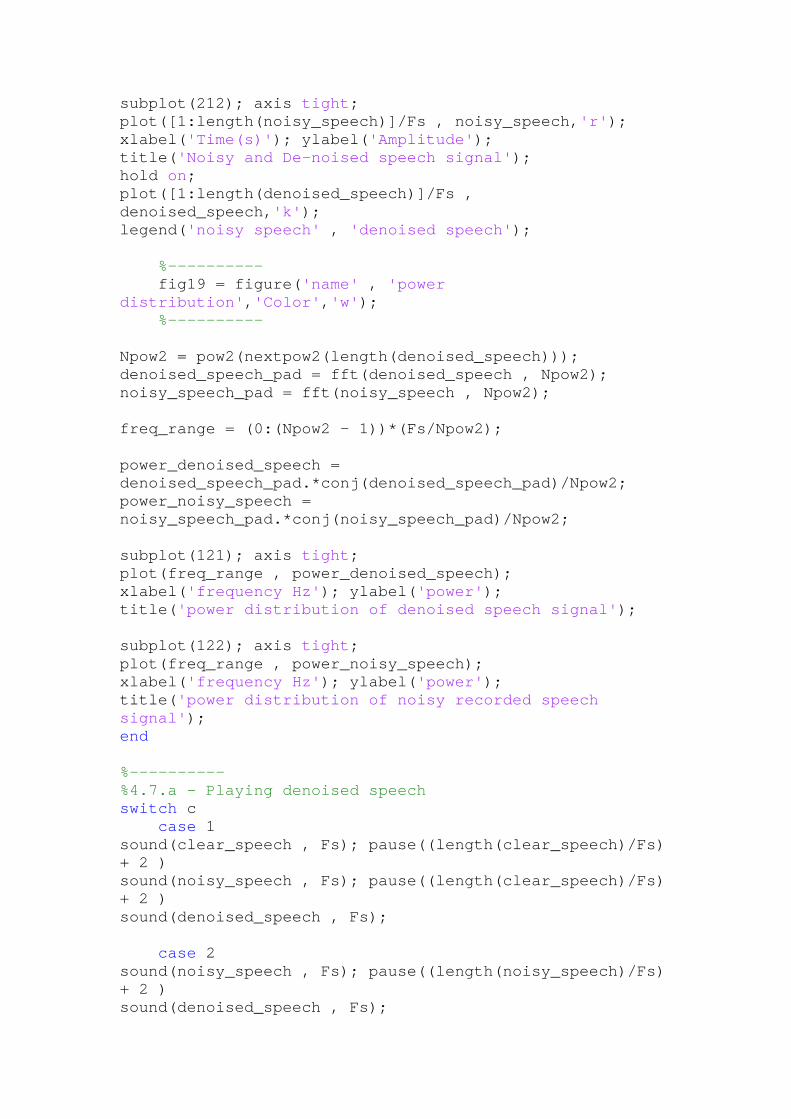
subplot(212); axis tight;plot([1:length(noisy_speech)]/Fs , noisy_speech,'r');xlabel('Time(s)'); ylabel('Amplitude');title('Noisy and De-noised speech signal');hold on;plot([1:length(denoised_speech)]/Fs ,denoised_speech,'k');legend('noisy speech' , 'denoised speech');

%----------fig19 = figure('name' , 'power

distribution','Color','w');%----------

Npow2 = pow2(nextpow2(length(denoised_speech)));denoised_speech_pad = fft(denoised_speech , Npow2);noisy_speech_pad = fft(noisy_speech , Npow2);

freq_range = (0:(Npow2 - 1))*(Fs/Npow2);

power_denoised_speech =denoised_speech_pad.*conj(denoised_speech_pad)/Npow2;power_noisy_speech =noisy_speech_pad.*conj(noisy_speech_pad)/Npow2;

subplot(121); axis tight;plot(freq_range , power_denoised_speech);xlabel('frequency Hz'); ylabel('power');title('power distribution of denoised speech signal');

subplot(122); axis tight;plot(freq_range , power_noisy_speech);xlabel('frequency Hz'); ylabel('power');title('power distribution of noisy recorded speechsignal');end

%----------%4.7.a - Playing denoised speechswitch c

case 1sound(clear_speech , Fs); pause((length(clear_speech)/Fs)+ 2 )sound(noisy_speech , Fs); pause((length(clear_speech)/Fs)+ 2 )sound(denoised_speech , Fs);

case 2sound(noisy_speech , Fs); pause((length(noisy_speech)/Fs)+ 2 )sound(denoised_speech , Fs);

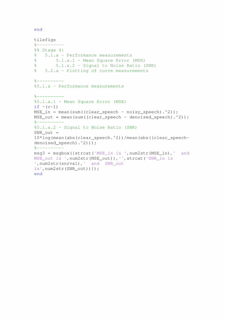
end

tilefigs%----------%% Stage 4:% 5.1.a - Performance measurements% 5.1.a.1 - Mean Square Error (MSE)% 5.1.a.2 - Signal to Noise Ratio (SNR)% 5.2.a - Plotting of curve measurements

%----------%5.1.a - Performance measurements

%----------%5.1.a.1 - Mean Square Error (MSE)if ~(c-1)MSE_in = mean(sum((clear_speech - noisy_speech).^2));MSE_out = mean(sum((clear_speech - denoised_speech).^2));%----------%5.1.a.2 - Signal to Noise Ratio (SNR)SNR_out =10*log(mean(abs(clear_speech.^2))/mean(abs((clear_speech-denoised_speech).^2)));%----------msg3 = msgbox({strcat('MSE_in is ',num2str(MSE_in),' andMSE_out is ',num2str(MSE_out)),'',strcat('SNR_in is',num2str(snrval),' and SNR_outis',num2str(SNR_out))});end

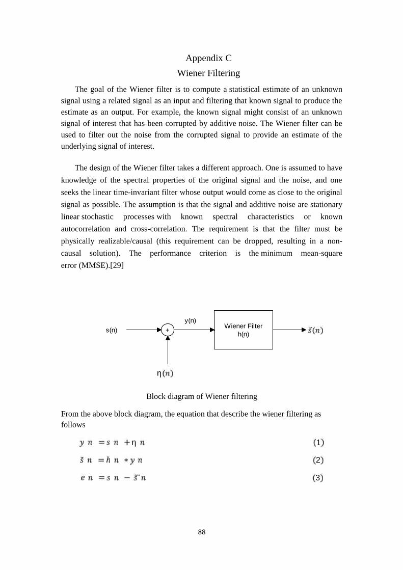
88

Appendix C

Wiener Filtering

The goal of the Wiener filter is to compute a statistical estimate of an unknown

signal using a related signal as an input and filtering that known signal to produce the

estimate as an output. For example, the known signal might consist of an unknown

signal of interest that has been corrupted by additive noise. The Wiener filter can be

used to filter out the noise from the corrupted signal to provide an estimate of the

underlying signal of interest.

The design of the Wiener filter takes a different approach. One is assumed to have

knowledge of the spectral properties of the original signal and the noise, and one

seeks the linear time-invariant filter whose output would come as close to the original

signal as possible. The assumption is that the signal and additive noise are stationary

linear stochastic processes with known spectral characteristics or known

autocorrelation and cross-correlation. The requirement is that the filter must be

physically realizable/causal (this requirement can be dropped, resulting in a non-

causal solution). The performance criterion is the minimum mean-square

error (MMSE).[29]

Block diagram of Wiener filtering

From the above block diagram, the equation that describe the wiener filtering asfollows

1 2 3

+ Wiener Filterh(n)s(n)

y(n)

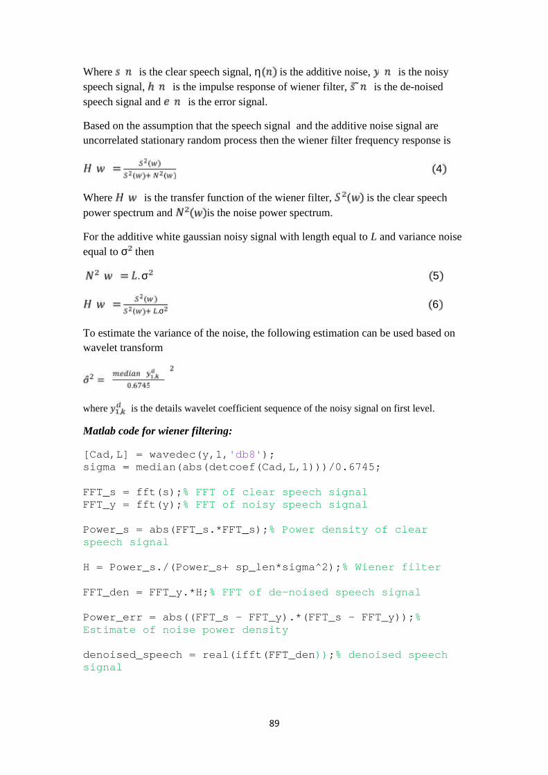
89

Where is the clear speech signal, is the additive noise, is the noisyspeech signal, is the impulse response of wiener filter, is the de-noisedspeech signal and is the error signal.

Based on the assumption that the speech signal and the additive noise signal areuncorrelated stationary random process then the wiener filter frequency response is4Where is the transfer function of the wiener filter, is the clear speechpower spectrum and is the noise power spectrum.

For the additive white gaussian noisy signal with length equal to L and variance noiseequal to then. 5

. 6To estimate the variance of the noise, the following estimation can be used based onwavelet transform

,.where , is the details wavelet coefficient sequence of the noisy signal on first level.

Matlab code for wiener filtering:

[Cad,L] = wavedec(y,1,'db8');sigma = median(abs(detcoef(Cad,L,1)))/0.6745;

FFT_s = fft(s);% FFT of clear speech signalFFT_y = fft(y);% FFT of noisy speech signal

Power_s = abs(FFT_s.*FFT_s);% Power density of clearspeech signal

H = Power_s./(Power_s+ sp_len*sigma^2);% Wiener filter

FFT_den = FFT_y.*H;% FFT of de-noised speech signal

Power_err = abs((FFT_s - FFT_y).*(FFT_s - FFT_y));%Estimate of noise power density

denoised_speech = real(ifft(FFT_den));% denoised speechsignal

90

References

[1] Pankaj Bactor, Anil Garg, ’’Different Techniques for the Enhancement of theIntelligibility of a Speech Signal’’, International Journal of Engineering Researchand Development, Volume 2, Issue 2 (July 2012), PP. 57-64.

[2] Steven F.Boll, ’’Suppression of Acoustic Noise in Speech Using SpectralSubtraction’’, IEEE TRANSACTIONS ON ACOUSTICS, SPEECH, AND SIGNALPROCESSING, VOL. ASSP-27, NO. 2, APRIL 1979.

[3] M. A. Abd El-Fattah, M. I. Dessouky, S. M. Diab and F. E. Abd El-samie ,’’SPEECH ENHANCEMENT USING AN ADAPTIVE WIENER FILTERINGAPPROACH’’, Progress In Electromagnetics Research M, Vol. 4, 167–184, 2008.

[4] Yariv Ephraim, Student Member,IEEE,and David Malah, Senior Member, IEEE,’’Speech Enhancement Using a- Minimum Mean-Square Error Short-Time SpectralAmplitude Estimator’’, IEEE TRANSACTIONS ON ACOUSTICS, SPEECH, ANDSIGNAL PROCESSING, VOL. ASSP-32, NO. 6, DECEMBER 1984.

[5] Xiaoqiang Xiao, Peng Lee, and Robert M. Nickel, ’’ INVENTORY BASEDSPEECH DENOISING WITH HIDDEN MARKOV MODELS’’, 16th EuropeanSignal Processing Conference (EUSIPCO 2008), Lausanne, Switzerland, August 25-29, 2008, copyright by EURASIP.

[6] Mark Klein and Peter Kabal, ’’SIGNAL SUBSPACESPEECHENHANCEMENTWITH PERCEPTUAL POST-FILTERING’’, Proc. IEEEInt. Conf. Acoustics, Speech, Signal Processing (Orlando, FL), pp. I-537-I-540, May2002.

[7] D.Gabor, ’’THEOREY OF COMMUNICATION’’, Britsh Thomson-Houston Co.,Ltd, Research laboratory, received 25th November, 1944.

[8] Stephane G. Mallat,’’ A Theory for Multiresolution Signal Decomposition: TheWavelet Representation’’, IEEE TRANSACTIONSO N PATTERNA NALYSISAND MACHINE INTELLIGENCE.V OL. II, NO. 7. JULY 1989.

[9] Stephane G. Mallat,’’ Multifrequency Channel Decompositions of Images andWavelet Models’’, IEEE TRANSACTIONS ON. Acoustics, Speech, and SignalProcessing VOL-37.NO.12.december 1989.

[10] Ingrid Daubechies, ’’ Orthonormal Bases of Compactly Supported Wavelets’’,AT&T Bell laboratories, received December, 1987.

[11] Stephane G. Mallat and Wen Liang Hwang, ’’SingularityDetection andProcessing with Wavelets’’,IEEE TRANSACTIONS ON INFORMATION THEORY,VOL.38,NO.2,MARCH 1992.

[12] David L.Donoho, ’’NONLINEAR WAVELET METHODS FOR RECOVERYOF SIGNALS,DENSITIES,AND SPECTRA FROM INDIRECT AND NOISYDATA’’, Proceeding of Symposia in Applied Margematics, VOL.00, 1993.

91

[13] David L. Donoho,’’De-Noising by Soft-Thresholding’’, TRANSACTIONS ONINFORMATION THEORY, VOL. 41, NO. 3, MAY 1995.

[14] David L. Donoho and Iain M. Johnstone,’’ Ideal Spatial Adaptation by WaveletShrinkage’’, Biometrika, 81, 425-455.

[15] Iain M.Johnstone and Bernard W.Silverman,’’Wavelet threshold estimators fordata with correlated noise’’,revision august 20,1996.

[16] Lawrence Rabiner, Biig-Hwang Juang, FUNDAMENTALS OF SPEECHRECOGNITION, PTR Prentice-Hall, Inc, Englewood Cliffs, New Jersey, 1993.

[17] S.ChinaVenkateswarlu, Dr. K.Satya Prasad, Dr. A.SubbaRamiReddy,’’ImproveSpeech Enhancement Using Weiner Filtering’’, Global Journal of Computer Scienceand Technology, Volume 11 Issue 7 Version 1.0 May 2011.

[18] RobiPolikar, THE ENGINEER'S ULTIMATE GUIDE TO WAVELETANALYSIS, 1999, available at

http://users.rowan.edu/~polikar/WAVELETS/WTtutorial.html

[19] R.J.E. Merry, Wavelet Theory and Applications A literature study, 2005.

[20] Brani Vidakovic and Peter Mueller, WAVELETS FOR KIDS A TutoialIntroduction, 1991.

[21] Andrew E. Yagle and Byung-Jae Kwak, THE WAVELET TRANSFORM:WHAT'S IN IT FOR YOU?,Presentation to Ford Motor Co., 1996.

[22] Bernhard Wieland, Speech Signal Noise Reduction with Wavelets, 2009.

[23] Ste'phane Mallat, AWavelet Tour of Signal Processing, Academic Press,USA,1998.

[24] Gilbert Strange and Truong Nguyen, Wavelets and Filter Banks, Wellesley-Cambridge Press, USA,1997.

[25]Gilbert Strange, Computational Science and Engineering, Wellesley-CambridgePress, USA,2007.

[26] Ole Christensen, Functions, Spaces, and Expansions : Mathematical Tools inPhysics and Engineering, Springer Science+Business Media LLC, USA, 2010.

[27] Michel Misiti, Yves Misiti, Georges Oppenheim and Jean-Michel Poggi,Wavelet Toolbox For Use With MATLAB, The MathWorks, Inc., 1996.

[28] www.mathworks.com

[29] wikipedia.org/wiki/Wiener_filter