de-noising of marine seismic data by steffen storbakk
TRANSCRIPT

Master Thesis, Department of Geosciences
De-noising of marine seismic data
By
Steffen Storbakk

De-noising of marine seismic data
By
Steffen Storbakk
Master Thesis in Geosciences
Discipline: Petroleum Geology and Geophysics (PEGG)
Department of Geosciences
Faculty of Mathematics and Natural Sciences
University of Oslo
June 2012

© Steffen Storbakk, 2012 Tutor(s): Prof. Leiv-J. Gelius, Dr. Charlotte Sanchis (FGAS) and Mark Rieder (FMCS).
This work is published digitally through DUO – Digitale Utgivelser ved UiO
http://www.duo.uio.no
It is also catalogued in BIBSYS (http://www.bibsys.no/english) All rights reserved. No part of this publication may be reproduced or transmitted, in any form or by any means,
without permission.


2
Acknowledgements This work has been carried out at Fugro Norway, situated in Oslo. I am truly grateful
for the opportunity I was given to write my thesis in collaboration with Fugro
Norway. First of all, I would like to thank Dr. Thomas Elboth, who proposed and
inspired me to write a thesis within the discipline of geophysics. Thank you for
believing and taking care of me from the very beginning.
A special thank goes to my external supervisors. Dr. Charlotte Sanchis for valuable
support and guidance during the processing and preparation of the thesis, and Mark
Rieder for critical feedbacks of the processing results.
Thanks to the processing staff at FSI, especially Martin Wahle and Yonghai Zhang
for helping me with technical questions, regarding data processing. Fugro Multi
Client Services (FMCS) AS for providing data for this thesis and generously allowing
me to publish the seismic data employed in this work.
I am immensely thankful for my internal supervisor, Prof. Leiv-J. Gelius at the
Department of Geoscience, for his invaluable encouragement, supervision and useful
suggestions throughout this thesis work. I deeply acknowledge his strong support in
order to raise the quality of this work.
Thanks to my fellow students, Uzma Mahmood and Pia Madeleine Lindstrøm for
interesting discussions and numerous lunch breaks at Fugro. Sindre Jansen, Bo
Haugan, Al-Amin Mazumder, Ibrahim Jalal, Danial Farvardini, Md. Jamilur Rahman
for their social contribution at the Department of Geoscience.
I also owe thanks to my mother, who is constantly worrying about when I should
finish my academic career and get a job. A big thanks goes also to my sister for her
love and support.
Last but not least, I am truly thankful for having my partner Nadja in my life and for
all her patience, unconditional love and support.
Oslo, June 2012
Steffen Storbakk

3
Abstract
Marine seismic acquisition represents one of the most used geophysical exploration
techniques employed in the petroleum industry today. However, one major challenge
is that marine seismic data will be distorted by a certain amount of noise originating
from various sources.
This thesis will look for an optimized de-noising flow of a marine seismic line that
was discarded (scrapped line) because the noise threshold values were considered to
be too high. This line was then reacquired (reference line) and is going to be
processed along with the discarded line and simultaneously serves as a benchmark.
The main objective of this work is to see if it is possible to raise the quality of the
scrapped data during processing so that it resembles the quality of the reference data.
Since seismic processing techniques have evolved significantly within the last
decades, it might thus be acceptable to acquire data in rougher weather conditions.
Accordingly, the noise threshold values could be adjusted.
After extensive testing, an optimized de-noising combination was identified. When
applied to the scrapped line as well as the reference line, very similar results were
obtained. Both visual inspection and calculated RMS values have been taken into
account to assure the quality of the final results. These observations support the basic
idea of accepting more noise in future marine acquisitions, due to advances in seismic
processing (e.g. de-noising).

4
Abbreviations
CO - Common offset
CDP - Common depth point
FBLP - Forward-backward linear prediction
FREC - Field record
LSE - Least squares error
NLMS - Normalized least mean square
NMO - Normal move-out
MMSE - Minimum mean square error
POSTM - Post migration
QC - Quality Control
RMS - Root mean square
SI - Seismic interference
SNR - Signal-to-noise ratio
SP - Shot point
SSTN - Shot station
TWT - Two-way travel time

5
Content ACKNOWLEDGEMENTS ................................................................................................................... 2
ABSTRACT ........................................................................................................................................... 3
ABBREVIATIONS ............................................................................................................................... 4
CONTENT ............................................................................................................................................. 5
1. INTRODUCTION ............................................................................................................................ 7 1.1. OUTLINE OF THE THESIS ......................................................................................................................... 7 1.2. OBJECTIVES AND MOTIVATIONS ............................................................................................................ 7
2. SEISMIC NOISE IN MARINE ACQUISITION ............................................................................ 9 2.1. COHERENT NOISE .................................................................................................................................. 10
2.1.1. Non-linear coherent noise ............................................................................................................ 10 2.1.2. Linear Coherent Noise.................................................................................................................... 11 2.1.3. Swell Noise........................................................................................................................................... 12
2.2. NON-COHERENT NOISE (RANDOM NOISE) ........................................................................................ 14
3. DE-NOISING METHODS .............................................................................................................15 3.1. COMMONLY USED METHODS FOR RANDOM NOISE ATTENUATION ................................................ 15
3.1.1. Frequency Filtering ......................................................................................................................... 15 3.1.2. F-X prediction filtering .................................................................................................................. 17
3.2. COHERENT NOISE REMOVAL TECHNIQUES ........................................................................................ 22 3.2.1. SWELL ................................................................................................................................................... 22 3.2.2. TFDN (Time Frequency De-Noise) ........................................................................................... 24 3.2.3. MINC (Multiple-Input adaptive seismic Noise Canceller) ............................................. 28
4. DATA PROCESSING ....................................................................................................................32 4.1. DATA ....................................................................................................................................................... 32
4.1.1. Scrapped Line (434060A-033) ................................................................................................... 35 4.1.2. Reference Line (434060B-048) .................................................................................................. 39
4.2. PROCESSING WORKFLOW ..................................................................................................................... 43 4.3.1. Pre-processing ................................................................................................................................... 44 4.3.2. Designature, resampling and scaling ..................................................................................... 44 4.3.3. De-noising ............................................................................................................................................ 45 4.3.4. Tau-P ...................................................................................................................................................... 46 4.3.5. Stacking ................................................................................................................................................ 47 4.3.7. Migration ............................................................................................................................................. 47

6
5. RESULTS ........................................................................................................................................49 5.1. SCRAPPED LINE (434060A-033) .................................................................................................... 49
5.1.1. Testing of the modules ................................................................................................................... 49 5.1.2. Optimized de-noising combination .......................................................................................... 52
5.2. REFERENCE LINE (434060B-048) ................................................................................................. 57 5.2.1. Optimized de- noising combination ......................................................................................... 57
5.3. COMPARISON OF THE SCRAPPED LINE AND THE REFERENCE LINE ............................................... 62
6. DISCUSSION ..................................................................................................................................71
7. CONCLUSIONS ..............................................................................................................................74
REFERENCES .....................................................................................................................................75
APPENDIX A: TIME DOMAIN VS FREQUENCY DOMAIN ......................................................78
APPENDIX B: CALCULATION OF RMS VALUES ......................................................................81 APPENDIX C: APPLICATION OF MINC AND TFDN ................................................................83
C.1. SCRAPPED LINE ..................................................................................................................................... 83 C.2. REFERENCE LINE ................................................................................................................................... 87

7
1. Introduction
1.1. Outline of the thesis This thesis was carried out in collaboration with Fugro Norway. It covers some of the
aspects of de-noising of marine seismic data and how selected de-noising tools can
improve the image of the subsurface.
The first chapter presents a short overview and the main objective of this thesis. The
second chapter provides some basic information about typical types of noise that may
be acquired along with the useful part of the marine seismic data. Chapter 3 presents
the main de-noising techniques that have been tested during this work, including a
new de-noising module that is yet to be released. Examples of both coherent and
random noise attenuation will be presented here. The seismic data to be processed and
analysed is introduced in Chapter 4. A flow chart describing the main steps in the 2-D
marine processing sequence is included. Chapter 5 presents the main results obtained
from the processing of both marine lines (pre-stack and post-stack). A closer
comparison of the output quality of these two lines is also included in this chapter.
Chapter 6 gives a short summary and discussion of the main results that were
obtained. Finally, chapter 7 states the main conclusions that follow from this study.
1.2. Objectives and motivations This thesis focuses on noise in marine seismic data. When the noise level on a marine
line exceeds a predetermined threshold, it is common practice to scrap that line and
reacquire the data once the noise level (usually caused by bad weather) has come
down. The noise threshold is typically defined by a seismic RMS-level of 15-
20 𝜇𝐵𝑎𝑟, after applying a 6-8 Hz low cut filter. This threshold has been part of
standard contracts for at least 20 years. However, both signal processing technologies
and computer power have improved considerably during this period, and today new
processing tools enable us to attenuate noise both quicker and more efficiently.

8
The objective of this thesis is to re-process a 2-D seismic line recently acquired in the
Barents Sea. This line was acquired twice, since the amount of noise was judged to be
too high during the first acquisition.
The work consists of combining existing and newly developed de-noising techniques
available in Fugro to attenuate as much as possible the noise contained in both the
scrapped line and the reference line. The final images will be compared to check if the
processed scrapped line (434060A-033) can achieve the same quality as the reference
line (434060B-048).
Furthermore, the work may provide objective arguments for accepting more noise in
seismic data during acquisition in the future. It is also expected that the available de-
noising tools are robust enough to remove the noise in the dataset of the scrapped line,
and match the quality of the reference line.

9
2. Seismic noise in marine acquisition
The data that is acquired in marine surveys can always be decomposed into a signal
and a noise component, the main objective being to recover the signal component. In
order to recover only the signal component, the noise component needs to be removed
from the data. However, the separation of the signal and noise is not a straightforward
process and may be challenging considering the diversity of noise types and
characteristics. There is no simple universal algorithm that can remove all the
different types of noise during the seismic data processing stage (Elboth et al.,
2009b). Nevertheless, efficient noise attenuation techniques exist and these become
more important as the demands of high-quality imaging are growing.
In order to define noise, one can say that: “any recordings that interfere with the
signal of interest can be considered as noise” (Elboth et al., 2009b). This chapter
introduces different types of seismic noise that may corrupt the data collected in
marine seismic acquisition. According to Yilmaz (2001), seismic noise can generally
be classified into two categories – coherent noise (linear– and non-linear) and
random noise (ambient noise).
Noise in seismic data is a significant problem for survey companies, especially
weather-induced noise that may result in delays. These delays can, according to Smith
(1999), account for up to 40 % of the total costs of a marine survey. In such cases, it
is also important from an economical point of view to be able to identify and attenuate
specific types of noise that corrupts the data of interest.
In some cases, it can be difficult to discriminate the noise from the data because it
may contain the same frequencies as the actual seismic reflection data, e.g. swell
noise and random noise. However, several different techniques are specifically
designed to attack different types of noise. The final challenge is often represented by
a trade-off between high quality imaging and computational time and costs.
Multiples, ghosts, diffractions, refractions, and random noise (e.g. wind, rain, tides)
are all different types of noise that we try to get rid of in the acquired data. These
types of noise are briefly described in the following sections. This work focuses

10
essentially on how to deal with random noise and swell noise in terms of seismic data
processing. This issue will be further discussed in section 2.3. The main de-noising
tools that are employed, in order to attack and attenuate these types of noise, are
TFDN, SWELL, RANNA and MINC. They are presented and discussed in Chapter 3.
2.1. Coherent noise According to Kearey (2002) and Ashton (1994), coherent noise represent components
of waveforms that are generated by the seismic source and that can be related to the
seismic equipment during a marine seismic survey. They can be further categorized in
non-linear coherent noise and linear coherent noise.
2.1.1. Non-linear coherent noise Water bottom multiples (reverberations) are defined as the energy that is propagating
down to the seabed from the shot, and then repeatedly reflected at the sea surface and
the seabed. Due to large differences in acoustic impedance (product of the velocity
and density), the reflection from these two interfaces are considered to be strong and
will cause reverberations in the seismic response (Gelius and Johansen, 2010;
Olhovich, 1964).
Ghost reflections can be considered as a special case of multiple reflections, and are
one of the most common forms of undesirable energy associated with marine seismic
acquisition. They are defined as reflections of the energy that is propagating towards
the sea surface from the shot. Since the sea surface may appear as a perfect reflector
(calm sea), the reflection energy propagates towards the seabed with a delay relative
to the primary. On the source side, these downward travelling waves will interfere
with the direct waves from the airgun array. On the receiver side they will interfere
with the upward travelling waves from the subsurface.
Figure 1 (left) illustrates how the ray paths of the multiple reflections (reverberations)
may propagate in the water column. The right part of the same figure shows how
ghost reflections are generated both at the source and receiver sides.

11
2.1.2. Linear Coherent Noise Diffractions are considered to be waves that are caused by irregularities on the
seafloor, or associated with subsurface features like faults, wedges, pinch-outs
(Olhovich, 1964). Imagine these features to be single points that reflect energy back
from all directions in depth, as shown in Fig. 2 (left). The corresponding zero offset
seismic section shown in Fig. 2 (right), will map the amplitude response of each trace
along the path of a diffraction hyperbola in zero offset time. In theory the diffraction
hyperbolas extend to infinite time and distance, however, in practice, they will as
mentioned, appear as truncated hyperbolic summation paths (Rastogi et al., 2000). If
the diffractions are located far from the sail line and/ or receivers, their seismic
response will be dominantly linear. Fig. 3 illustrates how these diffraction hyperbolas
can be identified in a seismic section.
Figure 1: Left: An example of multiple reflections (or reverberations). Right: An example of ghost reflection (Fugro internal training notes, 2012)
Figure 2: Schematic illustration of a point diffractor (left) and how the amplitude response of each trace will be mapped along the path of a diffraction hyperbola (right) (modified from Stein and Wysession, 2003)

12
Refractions (Fig. 4) occur when a layer, which may be a good transmitter, is emitting
energy to the surface due to interruptions within the layer, e.g. faults. The energy will
then be reflected back along nearly straight lines. The angle of incidence must reach
that critical angle before such refractions take place. In seismic data the refraction
will appear as straight lines crossing the seismic data.
2.1.3. Swell Noise Swell noise can be difficult to put in a category. Given the definition of coherent noise
provided earlier, it is practically impossible to reproduce it. Neither would it fit the
definition of random noise (section 2.2). However, based on the characteristics in the
amplitude spectra, swell noise is defined as a sub-category of coherent noise.
Figure 3: Illustration of how diffraction hyperbolas may look in a seismic section (modified from Kearey, 2002)
Figure 4: Schematic illustration of a two-layer model illustrating how the refracted wave is propagating in a good transmitter (medium 2), and where interruptions cause the energy to reflect back to the surface in nearly straight lines (Kearey, 2002).

13
Swell noise typically arises from rough weather conditions during marine seismic
recordings, especially in shallow waters. This weather-related noise has large
amplitudes at low frequencies and is spatially coherent over a number of hydrophones
(Elboth, 2010). It is directly related to the hydrostatic pressure fluctuations (height of
the water column above the streamer). The ocean waves induce cross-flow and vortex
shedding over the streamer (typically for the range from 2-15 Hz). Another
mechanism that may generate swell noise is bulge waves (transversal waves) induced
by the streamer motion. These are known to generate high amplitude noise up to 10
Hz. However, modern foam filled streamers are less affected by such bulge waves
(Elboth and Hermansen., 2009a). It is actually these phenomena (cross-flow, vortex
shedding and bulge waves) that are causing the swell noise that appears in the seismic
data. The reason why it appears as “blobs” which are increasing with time is due to a
scaling function that is normally applied to the dataset in the pre-processing step.
However, the high amplitudes are usually of low frequency and can typically be
removed by a low-cut filter.
According to Presterud (2009), swell noise can roughly be divided into two groups;
the first one is noise that has been generated from a distance away (direct ocean
swells). This type is characterized by very low frequencies, long wavelengths and
high amplitudes, and may be categorized as coherent noise. The other type is
generated by wind and storms at the actual survey site, leading to higher frequencies,
higher amplitudes and shorter wavelengths. Both types typically cover a large number
of neighbouring traces and appear as “blobs” in the data, with long wavelengths, high
amplitudes and relatively long periods. Fig. 5 shows how the swell noise typically
would appear in a shot gather. Note the high amplitudes that are corrupting major
parts of the dataset.

14
2.2. Non-coherent noise (random noise) Random noise (ambient noise) is a term given to the unpredictable part of the data,
whose amplitude is relatively flat in the frequency band of the signal (i.e. contains all
frequencies) and cancels out when traces are stacked together. This type of noise is
considered to be uncorrelated, whereas the signal is correlated (Elboth et al., 2010)
and usually not related to the survey itself (Kearey, 2002). This implies that the sum
of 𝑛 signals generally improves the signal-to-noise ratio (SNR) of √𝑛 (Elboth et al.,
2010).
Background noise like rain, wind, tides, vibrations of machinery, noise from
production platforms, etc. are generally characterized by high frequencies. Normally,
these high frequencies are not lying within the signal bandwidth and can be removed
by employing low-pass and band-pass filters (Gelius and Johansen, 2010; Yilmaz,
2001; Olhovich, 1964). As mentioned before, stacking is usually an efficient method
to attenuate random noise within the frequency band of the signal. F-X prediction
filtering may also be an alternative method that can be employed. The two latter
methods are discussed later and examples will be presented to illustrate how random
noise can be attenuated.
Figure 5: Shot gather contaminated with large amount of swell noise.

15
3. De-Noising Methods
There are different methods that can be employed in order to remove the noise in the
acquired data. The challenge is to employ the right method or the right combination of
methods, while at the same time leaving the real data virtually unaffected (Elboth,
2010). This chapter presents selected de-noising methods that we have chosen to
apply in this work. RANNA and TFDN are applied in order to attenuate random noise
whereas SWELL and MINC, in addition to TFDN, are specifically designed to
attenuate coherent noise. The aim is to attenuate both coherent and random noise and,
more specifically, swell noise. It is however important to be aware of other potential
or promising techniques, but it would surely go beyond the scope of this thesis to
present them all.
In seismic data processing, noise attenuation techniques can be performed in different
domains, e.g. shot domain, common offset (CO) domain or common depth point
(CDP) domain. Some of the techniques that are used work in the Fourier domain, and
a short discussion of time domain versus frequency domain can be found in Appendix
A. The purpose of the Fourier transformation is to ease the separation of the signal
from the noise (e.g. computational efficiency, simplified equations, filters based on
spectral shaping). However, note that frequency domain may not always be better
than time domain.
3.1. Commonly used methods for random noise attenuation In order to increase the SNR, one of the most important challenges in seismic data
processing is attenuation of random noise. In this section, two methods that are
specifically designed to suppress random noise are presented.
3.1.1. Frequency Filtering Random noise is commonly removed by employing frequency filters like low-pass
(high cut), high-pass (low cut) and/ or band-pass filters. Frequency filtering is an
efficient method to remove frequencies that does not fall in the frequency band of the
signal.

16
A low-pass filter allows low frequencies to pass up to the cut-off frequency, and
totally suppresses frequencies above the cut-off frequency. A high-pass filter is the
complementary of a low-pass filter, and removes the signals with lower frequencies
than the cut-off frequency, leaving the frequencies inside the reflection frequency
band untouched. A band-pass filter is a combination between a low-pass- and a high-
pass filter. It can be used to remove both low and high frequencies in the seismic data
where all the frequencies within the specified bandwidth pass at the same time (Gelius
and Johansen, 2010). Illustrations of these frequency filters are shown in Fig. 6.
The filtering process is carried out as a multiplication in the frequency domain and as
a convolution in the time domain. This operation may typically result in an increased
SNR. However, many components of seismic noise may lie within the frequency
spectrum of the reflected pulse, and cannot be attenuated by frequency filtering. A
typical bandwidth of the signal would be in the range of 10-70 Hz (Yilmaz, 2001).
Figure 7 shows an example from ProMAX, employing Ormsby filter, defined by four
corner frequencies (trapezoidal shape). The four corner frequencies were set to 5, 10,
55 and 65 Hz, designed to remove all frequencies below 5 and above 65 Hz. This is a
recursive one-sided filter, and by employing this band-pass filter, the SNR increases
and the quality of the CMP gather is improved. The improvements are predominantly
between 600-2800 ms and 3200-5000 ms. Both swell and random noise are
attenuated.
Figure 6: Schematic illustration of frequency filters: a) low-pass filter (high cut). b) high-pass filter (low cut). c) band-pass filter (modified from Gelius and Johansen, 2010).

17
3.1.2. F-X prediction filtering F-X prediction filters, also known as F-X deconvolution, are well understood. It is
one of the most common techniques to attenuate noise, and was originally proposed
by Canales (1984). He demonstrated how a complex one-step-ahead prediction filter
could be used to reduce random noise in stacked seismic data. The general idea was
to exploit the signal predictability in the spatial direction. Linear and noise free events
in the time-offset domain could be recognized as perfectly predictable events of
harmonics in the frequency-offset domain (Bekara and Van Der Baan, 2009). This
means that the signal that is being processed or analysed is assumed to be stationary,
meaning that their statistical properties are not varying with time (Hayes, 1996).
The next section is adapted from the thesis work of Presterud (2009) to illustrate the
principles of this technique.
Assume a sampled seismic pulse 𝛿(𝑡) so that a linear event in space and time can be
described as:
𝑓(𝑥, 𝑡) = 𝛿(𝑎 + 𝑏𝑥 − 𝑡) (3.1)
Figure 7: Illustration of the CMP gather before (left) and after (right) band-pass filtering. Scaling and muting has been applied to the CMP gather prior to the band-pass filtering. Improvements can be seen both in the upper and the deeper parts.

18
After Fourier transformation with respect to time, the equation becomes:
𝑓(𝑥, 𝜔) = 𝑒 ( ) = 𝑒 [𝑐𝑜𝑠(𝜔𝑏𝑥) + 𝑖𝑠𝑖𝑛(𝜔𝑏𝑥)] (3.2)
where 𝜔 is the angular frequency. As we can see from Eq. (3.2) the function is
periodic in 𝑥 for a simple linear event.
If a sampling ∆𝑥 is introduced along the x-coordinate, it becomes:
𝑈 = 𝑓(𝑥 , 𝜔) = 𝑒 ( ∆ ) 𝑛 = 1,2,3, . . . , 𝑁 (3.3)
where 𝑁 represents the total number of traces considered.
Assuming that 𝜔 is constant, 𝑈 can be predicted from the adjacent trace as follows
from Eq. (3.3).
𝑈 = 𝛼 ∙ 𝑈 , 𝛼 = 𝑒 ∆ (3.4)
The equation shows how this event is perfectly predictable with a complex Wiener
filter. In practical terms, the module proceeds as follows:
1. Transform a group of traces (a time series) from time-offset domain (t-x
domain) to the frequency-offset domain (F-X domain) applying Fourier
transform. For each frequency, a complex Wiener filter derived from the
autocorrelation function is generated and convolved with the input trace
(Galbraith, 1991) to give:
i. A prediction of the amplitude and the phase of the next trace where the
noise is the unpredicted part. It is only the centre trace in each group of
traces that will be output, because it is predicted by the adjacent traces
in the group. This is an iterative process where the signal is predicted
while the rest is considered as noise.

19
ii. Prediction of each trace is done twice, i.e. a forward and reverse
direction. The output sample for this frequency would be the average
value by forward and reverse prediction.
2. In this manner, predicted traces are reconstructed in the frequency domain and
then transformed back to the time domain.
This method makes it possible to discriminate the noise from the signal within the
same frequency band. The effect is usually a shortening of the pulse length, since
noise effects usually lengthen the seismic pulse. The shortening of the pulse length
will improve the vertical resolution.
Processing complex geological sections may, however, be a challenge for this
technique due to the assumptions of a stationary signal and local linear events. It gives
fairly good results for random noise attenuation but is not amplitude preserving.
A special implementation of the F-X prediction filter is employed here and is denoted
as RANNA (Random Noise Attenuation). It is a commercial de-noising method that is
based on forward-backward linear prediction filtering (FBLP) by Tufts and
Kumaresan (1982). It works more or less by the same principles as F-X prediction
filtering, which originally was proposed by Canales (1984). The difference, however,
is that the F-X prediction is optimum in a minimum mean-square error (MMSE)
sense, while RANNA is optimum in a least-squares error (LSE) sense, that is the
minimization of the sum of the squares of the estimation error. It is normally applied
after NMO correction to process shot records, common-offset sections or stacked
data.
When testing de-noising tools in this study, we experienced difficulties in applying
RANNA successfully in such an early process. Block size settings in the pre-stacked
data were set to be low (5 traces) to ensure that the events were locally linear. The
filter was also applied to the whole dataset, with a sliding window length of 200 ms in
order to reduce the runtime. It was applied in the CDP domain after normal move-out
(NMO) correction, but the obtained results were rather poor. The module removes
swell and random noise, but also significant amounts of the shallow coherent events.
Fig. 8 shows the results obtained after these settings were applied (CDP 1000). It was

20
neither applicable in the shot domain, as compared to the other de-noising modules,
nor the CO domain. This module is therefore not considered to be suitable as a de-
noising tool in any of the tested domains.
However, it was tested on a stacked section at a later stage and quite good results
were obtained. Significant amounts of random noise were attenuated and no linear
events could be observed in the difference plot (Fig. 9). Key parameters as the block
size was set to 100 traces and the filter was set to start from 3500 ms. The same length
of the sliding window (200 ms) was also applied. Note that another module was added
in the stack job to minimize the abrupt transition in the part of the stacked section
where RANNA was applied. The same procedure could actually have been applied
pre-stack in the CDP domain in order to preserve the linear events in the shallow
parts. This was not tested due to the limited amount of time.
Parameters used for the RANNA module are given in Table 1.
Figure 8: From left to right: Before, after and difference plots after RANNA has been applied in the CDP domain after NMO correction. A lot of noise has been removed in the difference plot, but also a significant amount of data.

21
Parameters Description RANNA The name of the module
FILT Specifies the filter length (in general between 3-9), the input traces per filter
prediction (block size), preferably a few hundred traces with the maximum
being 1024 traces, and white noise level in percentage (could be up to 30%).
WIND
Optional card: Defines the starting time (ms) and the length of the sliding
window (ms). Shorter trace length reduces the runtime.
OPTN Specifies the output data, filtered data (1) or removed data (2).
Table 1: A standard parameter file for the RANNA module.
Figure 9: From left to right: Before, after and difference plots after RANNA has been applied on a stacked section. SWELL and TFDN de-noising have been applied before the data was stacked.

22
3.2. Coherent noise removal techniques Swell noise is another significant problem experienced in marine data acquisition.
SWELL, TFDN and a new module denoted MINC are presented in this section. All
modules have proven to be well suited to attenuating this type of noise.
3.2.1. SWELL This module is specifically designed to suppress swell noise in marine data, and is
often a useful first step in eliminating band-limited noise. Swell noise is usually
characterized by rather constant amplitudes during the recording. This means that its
amplitude does not decay according to a “𝑇 pattern” (normally caused by spherical
divergence and attenuation as a function of time), but instead shows constant
amplitude levels during the recording. It can generally be characterized by long
wavelengths, high amplitudes and relatively long periods, typically in the frequency
range from 2-10(15) Hz (Elboth, 2010).
The algorithm decomposes each seismic trace into signal and noise components by
using a Butterworth filter specified by the user. The envelopes of both the signal and
the noise traces are subsequently calculated and compared with each other after
scaling adjustments. Whenever the noise envelope exceeds the signal envelope, the
noise is scaled down to match the signal level. Finally, the re-scaled noise
components and the signal components are added together to form a noise-attenuated
trace.
The Butterworth filter that is implemented in the
module is designed to have a frequency response
as flat as possible in the pass band, and rolls off to
zero in the stop band (Sanchis, 2010). It is
described in terms of two frequencies, FA and FB
and associated cut-off slopes SA and SB (Fig. 10). An attenuation of 3 dB, down from
the flat part of the pass band, will occur at the cut-off frequencies FA and FB. The
slopes are given in dB/ octave, where an octave represents a doubling of the
frequency. The doubling will typically result in lower values of the SB compared to
SA in order to make the filter well proportioned, if that is the case. Default values of
SA and SB are 18 dB/ octave and 36 dB/ octave respectively. They are generally
being considered as robust values suited to seismic data (Fletcher, 2009).
Figure 10: Illustration of the Butterworth filter that is implemented in the SWELL module.

23
Ideally, FA and FB should be set in the frequency range of where the presumed noise
is determined to be. A frequency range of 0-12 Hz is typical, as the swell noise mainly
affects these lower frequencies. However, in this case, the higher cut-off frequency
(FB) is adjusted down to 5 Hz, in order for the filter to perform well. Increases of FB
actually lead to heavier attenuation of the frequencies in the signal band where both
signal and noise were attenuated. Applying the filter to the whole dataset resulted in a
rather clean output, but some noise remains in the dataset. A suggestion for removing
the residual noise would be to combine SWELL with other modules, e.g. TFDN,
which has proven to be successful in many cases.
Figure 11 shows a typical example of a shot gather that is mainly contaminated with
swell noise. The FA and FB cut-off frequencies were set to 0 and 5 Hz respectively.
After the application of SWELL in the shot domain and CO domain, the low
frequency swell noise with abnormal high amplitudes has been attenuated. The output
result is significantly improved and the linear coherent events have been preserved.
Table 2 provides a short description of the main parameters in this module.
Figure 11: From left to right: Before, after and difference plots after SWELL has been applied. Note that the shot point (SP) has been sorted back to the shot domain, after the application in CO domain, in order to be able to make a residual plot.

24
Parameters Description SWELL The calling of the module
NOIS Defines FA and FB in the Butterworth filter, a scalar value used to down weight
data in the noise-band, and the length of the smoothing window (ms) respectively.
KEYS Optional card: Defines trace-header mnemonics to be used as primary and
secondary keys.
SWIN Optional card: Defines the window start of the processing. The end time is always
the end of the trace
Table 2: A standard parameter file for the SWELL module.
3.2.2. TFDN (Time Frequency De-Noise) The basic concept behind the TFDN algorithm is well known in the industry today,
and most seismic contractors have implemented some variants of this technique. It is
an adaptive algorithm that was initially designed to attenuate swell noise in marine
gathers. However, it turned out to be applicable to other types of noise as well, e.g.
seismic interference, propeller cavitation noise and strumming noise (Elboth, 2010).
The algorithm of TFDN has been presented both by Elboth et al. (2008) and Presterud
(2009). The idea behind this module is to:
1. Transform the data from time domain to frequency domain, where signal and
noise can be separated (e.g. employing Fast Fourier Transform (FFT)).
2. Remove or attenuate the noise in the frequency domain.
3. Transform the data back to the initial time domain (Inverse FFT).
The following section is adapted from the thesis work of Presterud (2009), and will
explain how the TFDN algorithm works in more detail.
The first step is to transform the data from time domain to frequency domain. To
transform the sampled signal, an FFT is normally applied, which is an optimized
method for computing Discrete Fourier Transform (DFT). Before computing the FFT,
a Hamming window is applied in order to minimize the signal side lobe effects. This
window is applied to all traces that are in a vertical window defined as inSlice.

25
In general, it is only selected parts of traces, defined by inSlice that are Fourier
transformed each time. In the frequency domain the TFDN algorithm considers all
traces in a horizontal sliding window defined inside inSlice (cf. Fig. 12). Inside this
horizontal window, the frequencies are investigated one by one (Fig. 13). Then, the
amplitude estimation of each frequency is compared with the amplitude estimate of a
presumed good trace. It is always the centre trace that is considered in the horizontal
sliding window (HWIN). If the centre trace amplitude (green) exceeds the user
supplied threshold values (purple), the amplitude becomes damped to the level of this
threshold attribute.
This process is repeated for all the frequencies specified by the user, and the modified
spectrum is then transformed back to the time domain (Inverse FFT). Then the
horizontal window is sliding one trace at a time until the whole horizontal range has
been covered. The vertical moving window, inSlice, is sliding to cover the next part of
the traces and the whole procedure is carried out again.
A user supplied threshold factor is applied in order to identify the anomalous
amplitudes. A threshold based on the median (MED) is normally being employed.
However, note that several other threshold calculations exists (e.g. lower quartile,
average, minimum, automatic). The median is normally applied if less than 50% of
the traces in the horizontal window (HWIN) are affected by noise:
𝑚𝑒𝑑𝑖𝑎𝑛 (𝑀𝐸𝐷) = (3.5)
Figure 12: An illustration of the horizontal sliding window, defined inside inSlice, after FFT (Presterud, 2009).

26
Figure 14 shows an example of TFDN applied to a shot gather (SP #1099). A typical
parameter file can be depicted in Table 3. Three iterations of TFDN were applied
using the median threshold value. The first iteration was set to filter the whole dataset
within the frequency range of 0-100 Hz. The next two iterations of TFDN were set to
follow the move-out curve of the first arrival to process frequencies in the range of 0-
14 Hz and 0-20 Hz respectively. The threshold factors were adjusted down for heavier
attenuation in the latter iterations of TFDN. However, the output result was not
completely successful. This may be connected to the theory behind the algorithm of
the TFDN. Here, the noisy traces are checked and compared with traces of the
neighbourhood. If the traces in the neighbourhood have high amplitude values, the
estimate of the data signal (presumed good trace) would not ideally be a good
estimate. Another reason might be that the parameters are not optimal set. However,
tests have proven that several iterations of TFDN with different parameter settings
and threshold values or combinations with other complementary de-noising modules
e.g. SWELL, improve the final output significantly. Sorting to another domain, e.g.
CDP and/ or CO domain, can break up the neighbourhood traces affected with large
amplitudes, and thus a better estimate of the data signal can be obtained (Elboth et al.,
2010). Nevertheless, this illustration provides a fairly good indication of how
effective the swell noise is attenuated while leaving the data of interest almost
unaffected.
Figure 13: The horizontal defined sliding window inside inSlice. This illustrates how the frequencies are checked for noise, one by one. The red ellipse marks a gathering of the amplitudes for one specific frequency and is sorted and finally damped if the amplitude exceeds the user defined threshold value (median based) (modified from Presterud, 2009).

27
Parameters Description TFDN The name of the module
TIMR Start and end time of the processing (ms)
FREQ Frequency range of processing (0-12 Hz)
HWIN Horizontal size of sliding window (no. of traces)
THRS Threshold card (e.g. median, lower quartile)
TWIN Optional card: vertical size of sliding window (ms)
Table 3: A standard parameter file for the TFDN module.
To get a better impression of the effects of the TFDN algorithm, an illustration of
TFDN applied to a single trace can be visualized, both in time and frequency domain
(Fig. 15). The input trace, before TFDN is applied, is shown in blue. It is affected by
large amplitude swell noise, especially from 4.5 s. The power spectrum of this trace is
characterized by an abrupt increase of energy in the 0-15 Hz interval caused by swell
noise, followed by a fairly flat characteristic over the frequency band before
decreasing towards the end. TFDN is then applied and the resulting trace is shown in
red - the swell noise has successfully been attenuated. The power spectrum shows that
the low frequency noise with high amplitudes have been significantly attenuated to
the user supplied threshold level. The red trace, obtained after TFDN, illustrates how
effective the algorithm attenuates the amplitudes of the lower frequencies (0-15 Hz).
Figure 14: Before, after and difference plot after 3 iterations of TFDN has been applied. The shot gather (SP #1099) is heavily contaminated with low frequency swell noise with abnormal high amplitudes.

28
3.2.3. MINC (Multiple-Input adaptive seismic Noise Canceller) MINC is a new processing module that has been applied in this work (Sanchis, 2010).
It is currently at a developing and testing stage and has the potential to be
commercially released in the near future.
This module is an adaptive method for attenuation of coherent noise, especially when
characterized by high amplitudes and low frequencies. It utilizes a normalized least
mean squares (NLMS) algorithm with a variable normalized step-size that is derived
as a function of instantaneous frequency (Sanchis and Hansen, 2011). A variable
normalized step-size is necessary in order for the filter to respond quickly to changes
in signal statistics. It uses multiple noise sequences to estimate the noise content in
each trace, extracted from a spatial window prior the first seismic reflection arrivals.
The estimated noise is then subtracted from the input trace resulting in a trace
attenuated in noise. Furthermore, this forms the mean-square estimate of the signal.
The MINC module proposed by Sanchis (2010) proceeds as follows:
Assume a seismic trace or primary channel with a value at time sample 𝑛, is denoted
by 𝑥(𝑛). The trace signal consists of the sum of a seismic signal 𝑠(𝑛) corrupted by
noise 𝑣(𝑛) and becomes:
𝑥(𝑛) = 𝑠(𝑛) + 𝑣(𝑛) (3.6)
The multiple-input adaptive noise canceller uses a set of 𝑀 noise sequences
𝑣 (𝑛), … , 𝑣 (𝑛) to predict the noise contained in the primary channel at time sample
𝑛, and then subtract it from the primary. If the input noise sequences are correlated to
Figure 15: Illustration of a trace before and after TFDN has been applied in time domain (left) and power spectrum (right). Abnormal amplitude anomalies at frequencies below 15 Hz have been attenuated.
29
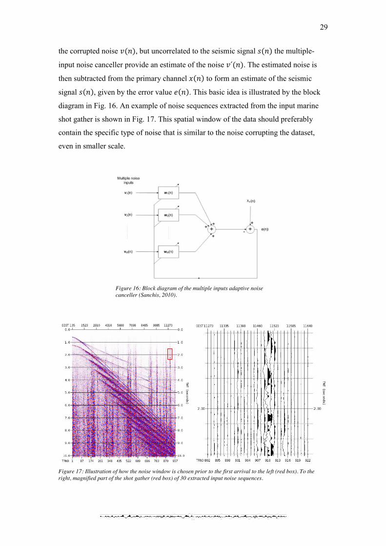
the corrupted noise 𝑣(𝑛), but uncorrelated to the seismic signal 𝑠(𝑛) the multiple-
input noise canceller provide an estimate of the noise 𝑣´(𝑛). The estimated noise is
then subtracted from the primary channel 𝑥(𝑛) to form an estimate of the seismic
signal 𝑠(𝑛), given by the error value 𝑒(𝑛). This basic idea is illustrated by the block
diagram in Fig. 16. An example of noise sequences extracted from the input marine
shot gather is shown in Fig. 17. This spatial window of the data should preferably
contain the specific type of noise that is similar to the noise corrupting the dataset,
even in smaller scale.
Figure 17: Illustration of how the noise window is chosen prior to the first arrival to the left (red box). To the right, magnified part of the shot gather (red box) of 30 extracted input noise sequences.
Figure 16: Block diagram of the multiple inputs adaptive noise canceller (Sanchis, 2010).

30
The error signal 𝑒(𝑛) forms the mean-square estimate of 𝑠(𝑛) and the NLMS
algorithm is used to determine a set of coefficient vectors that minimizes the mean-
square error at any time. The filter is operating with variable step-size (𝛽 , 𝛽 , 𝛽 ), in
order to adapt to the changing statistics of the seismic data. They are chosen with
respect to the instantaneous frequency content of each trace and the threshold values
provided by the user. Thus, for instantaneous frequencies smaller than the threshold
value, low frequency noise is detected and a large step-size should be used to
attenuate it. Conversely, for instantaneous frequencies larger than the threshold value,
seismic reflections are detected and smaller step-size should be used to preserve the
signal. In the testing the step sizes were set to be low, typically 𝛽 = 5.10 , 𝛽 =1.10 and 𝛽 = 10.10 . The noise sequences used to estimate the noise content
prior to the first arrival were designed to be in the time interval 1.5-2.3 s two-way
travel time (TWT) and offset interval 11,3-11,6 km in shot gather (SP # 1099).
Two frequency threshold values have been used, both percentage values and
instantaneous frequency values (Φ and Φ ). Percentage threshold values were set to
Φ = 0.25 and Φ = 0.16 in the first iteration of MINC. Instantaneous frequency
values, indicated by the first application of MINC, were chosen as threshold values in
the second iteration, and set to Φ = 6.94 Hz and Φ = 0.92 Hz.
The same set of noise sequences is used for all applications of MINC and the result of
this application is illustrated in the shot domain, see Fig. 18 (SP #1099). The module
suppresses the swell noise successfully, however, some swell noise are still left in the
dataset. Some artefacts were also created during the processing, and these are mainly
observed in the water column (Fig. 18). A typical parameter file describing the
parameters used in this module is given in Table 4.

31
Parameters Description MINC The calling of the module
STEP Specifies the normalized step size values that determine the convergence rate of the
adaptive filter. Larger step size results in more important attenuation. Defined as
three values (𝛽 , β , β ) that governs the convergence speed.
NSWIN Selection of a spatial window that is similar to the corrupting noise.
IFTHR Specifies the type of instantaneous frequency threshold to be used. In percentage or
as instantaneous frequency values (Φ ,Φ )
FORDER Specifies the order of the adaptive Wiener filter, typically 50
EPSSET Defines how to set the regularization parameter to avoid ill-conditioning matrices.
BLOCK Percentage of overlapping between data blocks, block length (# of traces)
Table 4: A standard parameter file for the MINC module.
Figure 18: From left to right: Before, after and difference plots after MINC has been applied to a shot gather (SP #1099) contaminated with low frequency swell noise.

32
4. Data Processing In order to obtain a good geological understanding of the acquired data, they need to
be processed and conditioned before interpretation.
This chapter is going to present two datasets acquired in the Barents Sea: one
scrapped line (434060A-033) that was discarded because the root mean square (RMS)
level was considered to be too high, and a reference line (434060B-048), which is a
re-acquired line of the scrapped line.
The processing workflow applied in this investigation is explained in more detailed
and a description of each step is given. The raw data is processed to produce a seismic
section of the geological structures in the subsurface. This chapter will furthermore
give a brief explanation of all the software modules that are applied in this work.
These modules are all integrated in the commercialized processing software Uniseis
that is used by Fugro Seismic Imaging (FSI).
4.1. Data The work focuses on applying selected de-noising techniques to a scrapped line
(434060A-033) to see how much noise reduction that is achievable. The idea is to
investigate if the de-noising methods are powerful enough to make this possible. If so,
old datasets that have been discarded just a few years ago may be accepted for
production today. Delays in acquisition of seismic data related to bad weather
conditions may also decrease.
A re-processing of the reference line (434060B-048) that was acquired quite recently
in the same area is used as a benchmark, in order to see how far it is possible to
approach the quality of this new dataset acquired under good weather conditions.
Thus, quality control (QC) of the results achieved from the de-noising of the scrapped
line will be controlled both by visual inspection and by calculation of RMS values.
The procedure of how the RMS values have been calculated in this work is explained
in more details in Appendix B.
The two seismic lines have been acquired in the western Barents Sea located north of
Norway (Fig. 19). Since line 434060A-033 was aborted due to bad weather conditions

33
and generation of swell noise, it appears as a short line (white), while the reference
line (434060B-048) that was acquired without any delay and fully completed is
illustrated in black.
Since there are significantly more shot points in the reference line, the relevant part
resembling the scrapped line has to be identified. The original field record numbers
(FREC) and/ or the shot station number (SSTN) from the trace header were then
checked in order to pinpoint the correct positions of the respective lines. These FREC/
SSTN numbers usually coincide if data has been acquired in the same area. However,
it would never be possible to compare the locations exactly, due to the feathering
effects of the streamers at long offsets.
Figure 20 illustrates the main structural elements in the western Barents Sea and
possible target areas of where important structures are expected to appear. The
positions of the reference line (434060B-048) and the scrapped line (434060A-033)
are indicated here by the use of latitude and longitude information. It is also correlated
and adjusted compared to a base map provided by Fugro Multi Client Services
(FMCS). Based on this information it is possible to get an indication of which
structural area the lines are covering. Line 434060B-048 is starting from Bjørnøya
Basin (BB) and continues into the sub basin of Fingerdjupet (FSB) in a South-
Western to North-Eastern (SW-NE) trend. Line 434060A-033 is acquired in a
Figure 19: Location of the marine seismic survey. The white line represents the scrapped line (434060A-033) and the reference line (434060B-048) is illustrated in black (www.googleearth.com).

34
relatively flat area with no big vertical depth variations and between BB and FSB
with the same trend as the reference line. According to the regional profile (line 16)
with a semi parallel position (SW-NE trend) relative to both the acquired lines (Fig.
21), it is possible to determine upper Paleozoic sediments (Carboniferous-Permian
age) at a depth of 4 s TWT (Faleide et al., 2010). Based on this information, the
crystalline basement has to be at a greater depth, maybe 5-6 s TWT. However, it is
not easy to see any coherent events deeper than 4 s TWT. This information is also
supported by a fast track processing of the reference line provided by FMCS.
Figure 20: Main structural elements in the western Barents Sea and adjacent areas (Modified from Faleide et al., 2010). The illustration represents the positions of the scrapped line (white) and the reference line (black) that were acquired in the Western Barents Sea. The black line (16) represents a regional profile in a semi parallel manner to the seismic lines acquired in FSB.
BB = Bjørnøya Basin FSB = Fingerdjupet Sub-basin GH = Gardarbanken High HB = Harstad Basin HfB = Hammerfest Basin HFZ = Hornsund Fault Zone KFC = Knølegga Fault Complex KR = Knipovich Ridge LH = Loppa High MB = Maud Basin MH = Mercurius High MR = Mohns Ridge NB = Nordkapp Basin NH = Nordsel High OB = Ottar Basin PSP = Polheim Sub-platform SB = Sørvestnaget Basin SFZ = Senja Fracture Zone SH = Stappen High SR = Senja Ridge TB = Tromsø Basin TFP = Tromsø-Finnmark Platform VH = Veslemøy High VVP = Vestbakken Volcanic Province

35
To quantify the efficiency of the de-noising, two windows are selected in the post
stack seismic section before de-noising. One target area representing the shallow part
of the stacked seismic section and another target area that is representative for the
deeper parts. The target area in the shallow part is ideally expected not to change too
much, since these are events we normally do not want to attack with the de-noising
modules applied in this work (e.g. coherent events, dipping events). In the deeper
parts, some coherent events can be recognized down to 4-5 s TWT, supporting the
above analysis.
The target areas defined by these windows will likely contain data contaminated by
noise. Thus investigating the data falling inside the two pre-defined windows will
give indications on how well the de-noising has worked and how much noise that has
been attenuated.
4.1.1. Scrapped Line (434060A-033) The dataset consists of 1099 shot gathers. Each shot gather includes 960 traces with a
maximum fold of 240. The fold represents the maximum number of traces in a CDP
gather and is important when it comes to seismic resolution. A higher fold (F) will
naturally result in improved seismic resolution and can easily be calculated:
𝐹 = = ∙ .∙ = 240 (4.1)
Figure 21: Regional profile (16) in the Western Barents Sea (Faleide et al., 2010). See Fig. 20 for location and abbreviation.

36
where 𝑁 is the number of channels, Δ𝑔 the group interval and Δ𝑠 the shot interval. All
stacked sections in this work are represented as full fold CDP´s, in the CDP range of
1000-5300. The maximum recording time of the dataset is 10.1 s.
The original sampling rate was 2 ms, which implies 5051 samples per trace and 2526
samples per trace after resampling to 4 ms. A zero phase band-pass filter (Butterworth
type) with cut-off frequencies at 3 Hz and 95 Hz and corresponding cut-off slope
values of 18 dB/ octave and 72 dB/ octave were applied to the dataset. In addition, a
velocity and time dependent amplitude gain recovery (𝑉 𝑇) was applied to the
dataset in order to enhance deeper events relative to the shallower ones.
The last three shots that were processed (Fig. 22), i.e. shot points (SP) 1097-1099,
contain a significant amount of swell noise. The challenge is to find an optimized de-
noising flow that can attack not only swell noise, but all types of noise that are
identified. Besides swell noise, the following types of noise were identified in the shot
gathers: water bottom multiples, tugging noise and random noise (Fig. 22).
The unwanted coherent events represented by the linear parts of the reverberations, as
well as the linear tugging noise originated from the lead in cables and/ or from the
vessel propeller (Fig. 22, Box 1) are usually removed by tapering in the Tau-P
domain. The swell noise (Fig. 22, Box 2) is in this case supposed to be attenuated by
Figure 22: The last three shots SP (1097-1099) that were processed for the scrapped line. Identified noise: Tugging noise (box 1), swell noise (box 2), water bottom multiples (reverberations) and random noise in the illustration to the right.

37
employing one or several of the selected swell noise techniques. Random noise may in
general be attenuated by stacking and residual random noise may be attenuated by
employing e.g. RANNA and/ or Tau-P.
We produce a stacked section before de-noising (Fig. 23) in order to have a reference
stack to compare the de-noised results with. In the following discussions, the majority
of the results are presented post stack, with special emphasize on the two target zones
introduced earlier (Fig. 23). The idea is to zoom in on these target areas in order to get
a better understanding of the noise that is corrupting the data. Calculation of RMS
values will also give quantitative indications about de-noising in addition to visual
inspection within these zoomed areas.
High amplitude swell noise of low frequency is typically affecting the deeper parts,
while leaving the upper parts fairly clean. The target areas in Fig. 23 are illustrated
more closely in Fig. 24 (Box 1) and Fig. 25 (Box 2). In these magnified parts of the
seismic section it is possible to see how the amplitude responses look like prior to any
de-noising. The second target area (Box 2) is more affected by the identified noise
compared to the shallow target area (Box 1).
Figure 23: The stacked section after designature and prior to any de-noising. Box 1 and 2 show target areas to be investigated further.

38
Figure 25: Zoomed section corresponding to target area 2 of the scrapped line (left) and a small selected range of CDP´s (traces 2870-2880) (right) to illustrate the amplitude responses prior to any de-noising.
Figure 24: Zoomed section corresponding to target area 1 in the scrapped line (left) and a small selected range of CDP´s (traces 1740-1750) (right) to illustrate the amplitude responses prior to any de-noising.

39
4.1.2. Reference Line (434060B-048) The same pre-processing has been applied to the reference line as in the case of the
scrapped line. However, since the reference line was fully completed, more data has
been acquired. This line consisted originally of 7205 shot gathers (reduced to 1099
shots to match the scrapped line) with 960 traces in each shot gather and a maximum
fold of 240. The dataset has also a maximum recording time of 10.1 s. The
corresponding FREC numbers were extracted from this line to match the same
location as the scrapped line. The stacked sections will also be represented by full fold
CDP´s, in the range of CDP 1000 to 5300.
The original sampling rate was 2 ms, which implies 5051 samples per trace, and 2526
samples per trace after resampling to 4 ms. As in the case of the scrapped line, a zero
phase band-pass filter (Butterworth) with cut-off frequencies at 3 Hz and 95 Hz and
corresponding cut off slope values of 18 dB/ octave and 72 dB/ octave was applied to
the dataset. Scaling or amplitude gain was also applied (same as for the scrapped
line).
Compared to the scrapped line, this dataset appears fairly clean and is barely affected
by any weather-induced noise with abnormal high amplitudes. Fig. 26 shows the last
three shots of this reference line. Contrary to the last three shots of the scrapped line
(Fig. 22), no significant tugging noise or swell noise is visible. The noise content in
these three last shots of the reference line is very different. The main noise types
corrupting this dataset are random noise and massive reverberations. Some positive
dipping events (from ahead) identified as seismic interference (SI) are also recognized
and seem to appear occasionally in the shot gathers (Fig. 26). As it turns out, no
abnormal high amplitude noise exists in this dataset that requires correction. Thus, it
has to be treated differently from the scrapped line when setting the parameters in the
optimized de-noising sequence.

40
As mentioned earlier, the reference line will serve as a benchmark. Figure 27 shows
the stacked reference line prior to any de-noising. Again, the same two target areas as
for the scrapped line have been introduced (Box 1 and 2 in Fig. 27). Later
comparisons will be based on both visual inspection and calculated RMS values. The
RMS values of the reference line will indicate how much noise is acceptable. If the
final result of the scrapped line is in some way close to the reference line, the de-
noising of the scrapped line will be considered as successful.
Within the deeper parts (Box 2), the reference line is mainly troubled with random
noise masking possible structures deeper than 3-4 s TWT in the subsurface, while the
scrapped line is mostly affected by a combination between swell and random noise.
Figure 26: Last three shots of the reference data, SP 1097-1099.

41
The corresponding target areas of the reference line can be depicted in Fig. 28 and
Fig. 29 respectively, Box 1 representing the shallow parts and Box 2 representing the
deeper parts of the stacked section.
In general, there are no big differences in the shallow parts between the reference and
the scrapped seismic sections before de-noising has been applied. However, larger
differences can be seen in the deeper parts, in the time range between 3-5 s TWT.
Figure 27: The seismic stacked section of the reference line after designature and prior to any de-noising. Box 1 and 2 are target areas to be investigated further.
42
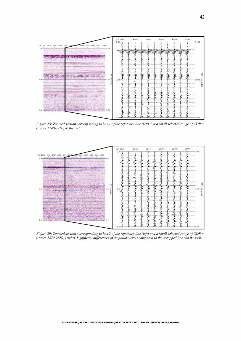
Figure 29: Zoomed section corresponding to box 2 of the reference line (left) and a small selected range of CDP´s (traces 2870-2880) (right). Significant differences in amplitude levels compared to the scrapped line can be seen.
Figure 28: Zoomed section corresponding to box 1 of the reference line (left) and a small selected range of CDP´s (traces 1740-1750) to the right.

43
4.2. Processing workflow Uniseis is the main processing software that is used by Fugro Seismic Imaging (FSI).
It encompasses all aspects of seismic data processing and has been used to perform all
the jobs in the processing flow. All modules are integrated in the software either as
stand-alone modules that are “independent” or as software families or suites.
It is important to keep in mind that a processing sequence is not fixed and may vary
from survey to survey. A flow chart of the 2D marine processing sequence that was
created for this project is presented in Fig. 30, followed by a brief description of each
step in the processing flow. The key step in the processing flow was the de-noising,
where the selected de-noising techniques have been tested extensively, often
determined by experience and trial and error. Accordingly, some of the processing
steps in the de-noising sequence have been repeated several times, stacked up and
migrated in order to compare the different outputs. Different approaches and
combinations of the de-noising modules have also been tested extensively in the
search for an optimized de-noising flow. The most promising modules are then going
to be applied to the scrapped and reference line.
Figure 30: The 2-D marine processing flow employed in the processing of the scrapped line (434060A-033) and the reference line (434060B-048).
44
4.3.1. Pre-processing The process starts by reading in the original input file of the shot gathers. The
sequence of the first and the last shot to process is given by the trace header and
defined in the processing flow. All values related to the geometry are also added into
the processing flow, such as interval distances (shot-point, hydrophones, near trace
number, shot to near trace offset distance) and distances (offset). This information can
for instance be used for calculating the CDP interval and the fold. A card that controls
re-sequencing is also added to the processing flow. This enables the user to define the
shot gathers that are going to be processed before data is output. An example of a raw
SP (SP #1), before any processing has been applied, is shown in Fig. 31, left.
4.3.2. Designature, resampling and scaling The next step in the process is to apply designature (signature deconvolution). The
purpose of this module is mainly to preserve the frequency content and to convert the
recording signature to its minimum phase equivalent without affecting the amplitude
spectra. Both minimum phase wavelets and zero phase wavelets are preferred.
However, most recordings acquired are mixed phase. The purpose of designature is to
convert this mixed phase wavelet into a preferable zero – or a minimum phase
wavelet, because they are considered to have important characteristics when it comes
to an interpretational point of view or uniqueness.
Resampling of the data provides an option of increasing or decreasing the data length.
In this case, a resampling from 2 ms to 4 ms will reduce the data to a smaller sample
rate. It is performed in the frequency domain where a “brick wall” zero phase anti-
alias filter is applied. This is basically assumed to be an ideal filter, where some
frequencies can pass unchanged whereas others are suppressed in order to perfectly
reconstruct the signal from the samples and to avoid aliasing.
In addition, a default pre-filter (zero phase Butterworth filter) has been applied, with
cut-off frequencies at 3 Hz and 95 Hz, and corresponding cut-off slopes at 18dB/
octave and 72dB/ octave respectively. The filtering applied at this stage is a rather
standardized processing step that is normally applied to all raw marine field data in
order to remove the low frequencies with abnormal high amplitudes (Fig. 31, middle).

45
After filtering, amplitude scaling is also applied to compensate for geometrical
spreading and other amplitude losses. A gain function is applied to the deeper and
weaker signals in order to enhance the reflection energy, whereas stronger signals in
the shallow parts receive less gain (Fig. 31, right). In this case, a time and velocity
dependent exponential gain recovery function has been applied (𝑉 𝑇).
At this stage the dataset is ready to be further processed after proper QC and more
sophisticated de-noising modules can be applied.
4.3.3. De-noising The main principles of the de-noising modules applied in this processing flow
(SWELL, TFDN, RANNA, MINC) have been described in details in Chapter 3. The
aim of the de-noising modules is to ideally remove any residual noise from the
dataset. In this case, the main emphasis has been on attenuating random and swell
noise. The different de-noising modules can be used separately or in combination.
Figure 32 gives an example of a noise contaminated source gather (SP #1099), taken
from the scrapped line, before and after de-noising, using a combination of SWELL
and TFDN. The result obtained is fairly good. All the abnormal high amplitudes
within the lower frequencies (0-5 Hz) have been successfully attenuated, without
affecting any coherent events.
Figure 31: Left: A raw shot (SP #1). Middle: the same shot after application of designature. Right: The same shot after application of scaling. The source gather consists of 960 traces.

46
4.3.4. Tau-P Tau-P is a module that is usually employed to remove linear dipping noise e.g. direct
arrivals and refractions, including tugging noise (observed in the shot gathers for the
scrapped line). This module transforms the seismic data to the Tau-P domain and
back again. A series of linear events in the dataset are collapsed to points in the Tau-P
domain. Moreover, hyperbolic events will fall along elliptical curves in the Tau-P
domain. The purpose of this transformation is to ease the attenuation of coherent
events. Figure 33 illustrates how the hyperbolic events are discriminated from linear
events by transforming the data from t-x domain to Tau-P domain. The coherent
linear events are easily recognized and can be muted or tapered, before it is
transformed back to time-space domain.
Figure 33: Schematic illustration of the linear and move out events in Tau-P domain (www.xsgeo.com)
Figure 32: Application of SWELL and TFDN. From left to right: Before, after and difference plot. (SP #1099 from scrapped data).

47
4.3.5. Stacking Stacking represents a summation of NMO corrected traces in a CDP gather and can be
considered as a de-noising method. A velocity field is needed for the NMO
correction. Events like linear and non-linear coherent noise that are not corrected, are
attenuated through destructive interference, while reflections are aligned and
enhanced by constructive interference. The NMO corrected traces in each CDP gather
are then stacked into a single trace by summing over the offset axis (Fig. 34), where
lower velocities have stronger curvatures than higher velocities.
More traces (larger fold) would typically improve the SNR. Due to the end effects
(taper-on and off), we have chosen the CDP range 1000-5300 in this work to ensure a
full fold stack.
4.3.7. Migration To image the subsurface more correctly and to
minimize distortions of the true geological depth
model, migration (imaging) is required. It aims at
moving reflected events e.g. diffraction
hyperbolas, dipping reflectors and bow-tie
structures into their true subsurface positions.
Figure 35 illustrates how these features are
geometrically repositioned in either space or time
to the location where the event occurred in the
subsurface rather than the location it was recorded
at the surface (Sanchis, 2010). Diffractions are
Figure 34: Illustration of the principles of NMO correction (Fugro internal training notes, 2010). The reflections are aligned horizontally using correct velocities and finally summed.
Figure 35: Illustration of the effects of seismic migration. a) diffractions are collapsed to points. b) dipping events get steeper. c) bow-ties are unwrapped.

48
collapsed to points (Fig. 35a), dipping events are moved up-dip and become steeper,
and triplications (bow-ties) associated with synforms are unwrapped (Gelius and
Johansen, 2010; Yilmaz, 2001).
Another example from Yilmaz (2001) illustrates how these features are relocated into
their correct geological position in a zero offset seismic section. Fig 36 shows the
stacked section before and after migration has been applied respectively (Fig. 36a and
b). Figure 36c illustrates how the dipping event (B) is moved up-dip to (B’) and how
the diffraction (D) is collapsed to a point (D’).
The module that has been used to migrate the data in this work is denoted DIFMIG
and is based on the Kirchhoff formulation (integral or
summation solution to the wave equation). It is a 2-D
Post Stack Time Migration (POSTM), aiming to
move the data in the seismic stacked section to their
correct positions, both in time and space (Fletcher,
2009). Migration is the principle technique for
improving the horizontal resolution (Brown, 2004).
Fig. 37 illustrates how the stacked data are summed
along the scattering traveltime curve for a given
image point in depth (Gelius and Johansen, 2010). Figure 37: Schematic illustration of the summing along a scattering traveltime curve (Gelius and Johansen, 2010).
Figure 36: A stacked section. a) before migration. b) after migration. c) sketch of moved events (modified from Yilmaz, 2001).
49
5. Results
This chapter presents all the main de-noising results that have been obtained. All
modules have been tested as a stand alone module in a de-noising workflow to check
how much noise each method possibly can attenuate. However, a combination of
several modules in a de-noising flow is a standard procedure in production and will
typically lead to improved results. Also, sorting the data in different domains may be
necessary to optimally attenuate residual noise. For instance, TFDN may give
disappointing results when the noise affects the neighbouring traces. In such cases,
applying TFDN in another domain where the traces appear more random (e.g. CO
domain) improves its efficiency.
Presentations of the de-noising results are given in section 5.1 (scrapped line) and
section 5.2. (reference line), and are mostly presented post stack. In section 5.3 a
detailed comparison between the two processed lines is carried out supported by RMS
values. This analysis will focus on the two target areas introduced in section 4.1.1 (cf.
two boxes in Fig. 22).
5.1. Scrapped Line (434060A-033)
5.1.1. Testing of the modules Running a series of tests with different parameter settings determines the final
parameters that are going to be used in a production. During the initial de-noising
tests, each of the selected de-noising modules (SWELL, TFDN, RANNA, MINC) was
tested stand-alone, in order to see how well each of them handled the noisy dataset.
We applied each module to SP data before they were systematically tested in the other
domains (except from MINC). The sorting did in general not result in any significant
improvements, because most of the noise was sufficiently removed in the shot
domain. Minor or insignificant effects were observed by sorting. However, good
results were obtained when SWELL was applied in CO domain.

50
As expected, TFDN provided good results in the shot domain. SWELL was giving
fairly good results as well in the shot domain with some residual noise being further
attenuated in the CO domain. RANNA was more challenging to apply, because no
optimized parameter values were found during the testing. The module did not
manage to provide good results in any domain, even after several attempts of
parameter adjustments. Another idea was to apply it after NMO correction in the CDP
domain, but the results were still poor (the shallow coherent events were still strongly
attenuated). However, Canales (1984) demonstrated that prediction filters could be
used to remove random noise in stacked seismic data. RANNA was therefore applied
on the stacked section, but this only resulted in insignificant improvements when
combined with Tau-P. Consequently, RANNA was not investigated any further
during this study. MINC was only tested in the shot domain due to the limited amount
of time, but is applicable in the other domains as well (CO and CDP domain). It was
tested successfully in the shot domain. However, some artefacts were created in the
MINC output, mostly prior to the first reflection (sea floor).
To summarize, SWELL has proven to be efficient both in the shot and CO domain,
and suppresses lower and higher frequencies with abnormal high amplitudes just as
expected. TFDN detects abnormal amplitude anomalies and attenuates them within
the frequency band of the data of interest. MINC appears to be very similar to
SWELL for our dataset, and attenuates coherent noise, especially high amplitudes and
low frequencies.
Table 5 gives a short summary of which domains the different modules have been
applied in. It also indicates which of the applications that have been applied
iteratively.
Module Domain
MINC (2 iterations) SP domain
SWELL SP domain and CO domain
TFDN (3 iterations) SP domain
Table 5: Schematic presentation of the applications that have been applied iteratively and in which domains.

51
Both visual inspections and RMS values have been taken into account when choosing
an optimized de-noising flow. The optimal combination of these modules will yield
the best final de-noising results. We tested both a combination of SWELL and TFDN,
and MINC and TFDN. These two de-noising combinations performed very similar
since both combinations consist of modules that complement each other. This is also
in accordance with earlier observations that SWELL and MINC perform very similar.
A de-noising approach where SWELL, TFDN and MINC were put in a de-noising
flow was also tested without any success. The dataset is rather clean after the
combination of SWELL and TFDN, and therefore, applying MINC did not bring any
significant improvements.
However, MINC is a module which is still under development and yet to be released.
From an objective point of view, it can easily compete with the SWELL module and
has the potential to be an efficient de-noising module in the future. However, some
artefacts were observed in both the shot gathers and stacked sections during the
testing of this module. These issues should be investigated in more detail in the
future. Another issue was the parameter settings that were found to be very
challenging. MINC performs well on shot gathers that are heavily contaminated with
swell noise, but may not work so well on shot gathers that are less affected. However,
the same problem arised when SWELL was applied to the reference line, but setting
softer parameter values solved this issue.
Computationally, it is not fair to compare the combination of MINC and TFDN with
SWELL and TFDN since MINC currently is only allowed to run on a developer’s
platform. However, MINC is considered to be acceptable for seismic processing. This
technique is more complex than a second order high pass filter, but requires fewer
operations than TFDN, hence less computationally demanding than TFDN (Sanchis,
2010).
Based on visual inspection and RMS values, it turned out to be a combination of
SWELL and TFDN that yields the overall best results. For this reason, this approach
is going to be investigated further and compared with the reference line. Fig. 38
shows a flow chart of the processing sequence that will be applied to both of the
seismic lines.

52
Regarding the MINC and TFDN approach, the main results are given in Appendix C
for completeness.
5.1.2. Optimized de-noising combination This section presents the results obtained applying the optimized
de-noising combination of SWELL and TFDN.
The stacked section of the original scrapped data before de-
noising is shown in Fig. 36. The two boxes indicate the target
areas to be investigated more closely in section 5.3. The
corresponding RMS values will also be calculated in these target
areas in order to quantify the de-noising results.
As discussed earlier, the input data were heavily contaminated
with different types of seismic noise, especially swell noise,
random noise, water bottom multiples and tugging noise. The lower cut-off frequency
was set to 5 Hz in order to preserve any possible events underlying the tugging noise.
Since tugging noise appears randomly, some of this noise may actually be attenuated
when stacking. Dipping events or linear noise, such as tugging noise, are also
attenuated by Tau-P at a later stage.
Within this optimized de-noising approach, SWELL was applied both in the SP
domain and CO domain, but most of the swell noise was already removed during the
first sorting. The SWELL module had a massive effect on the shot gather with most
of the low frequency swell noise (0-5 Hz) being suppressed. However, some noise
was still left in the dataset, characterized by higher frequencies and not easily
attenuated without affecting the frequency band of the signal or the tugging noise.
This is often the case in seismic data processing, where a conflict between several
requirements occurs.
The following parameters were applied for the SWELL module (Table 6) (SP and CO
domain):
Figure 38: Optimized processing flow.

53
NOIS KEYS SWIN
SWELL in SP domain 0,5,0.5,60 IWATTIM,ITRNO 500,1,100,960,100
SWELL in CO domain 0,5,0.5,60 IWATTIM,ITRNO 500,1,100,960,100
Table 6: Parameter values of the SWELL module in the shot domain and CO domain.
The low cut frequency was set to 5 Hz and the filter was applied to the whole trace
from 100 ms. For practical reasons, the dataset was sorted back to shot domain after
SWELL was applied in the CO domain.
TFDN was only applied in the shot domain, simply because most of the noise was
attenuated in this domain. Further application in the CO and CDP domain gave
insignificant results. Sorting into any of these two latter domains actually caused
attenuation of coherent events, even with soft parameter settings. The tests indicated
that it was sufficient to apply 3 iterations of TFDN in order to achieve good results
(see below for more details).
In case of TFDN, Table 7 summarizes the parameter settings. This module was
applied in the shot domain and in an iterative manner.
TFDN 1st iteration TFDN 2nd iteration TFDN 3rd iteration
TIMR 1 500,,1500, 12.5 500,,1500, 12.5
FREQ 0-100 Hz 0-14 Hz 0-20 Hz
HWIN 20 20 20
THRS MED,4.5,2.5 MED,2.2,1.5 MED,2.2,1.5
TWIN 500,20 500,20 500,20
Table 7: Parameter values of the TFDN module
The first iteration TFDN was applied to the whole dataset. The horizontal window
(HWIN) was chosen small in width to make sure that the attenuation of the amplitude
anomalies were done locally. Stronger attenuation was made in the deeper parts.
In the second iteration of TFDN the data window followed the move-out curve of the
seafloor reflection (assuming a water velocity of 1500 m/s). Lower threshold values
were set for stronger attenuation of noise appearing at longer travel times.
In the third iteration of TFDN, the data window was applied from the seafloor starting
at 500 ms too. The purpose with this iteration was to attack intermediate frequencies

54
with a larger frequency range. The same threshold values as in the second iteration
were applied, resulting in stronger attenuation at larger travel times.
An example of the result obtained using this optimized de-noising scheme for SP
#1099 is shown in Fig. 39. This source gather was chosen due to its large content of
swell noise. One can observe in the after and difference plot that most of the low
frequency and high amplitude swell noise have been attenuated.
Before stacking the data, Tau-P filtering was applied in the shot domain. In order for
Tau-P to work properly, the shots have to be fairly noise free. The stacked section
before de-noising is shown in Fig. 40, after SWELL, TFDN and Tau-P filtering is
shown in Fig. 41 and the corresponding difference plot in Fig. 42. Tau-P filtering
removes significant amounts of additional random noise and dipping events, resulting
in an enhancement of the seismic reflection events. Finally, the seismic image after
migration is shown in Fig. 43. Some coherent events have been unmasked in the
deeper parts of the migrated section (7-8 s TWT) assumed to be multiples. Notice
some of the diffractions curves in the shallower parts that ideally should have been
collapsed during the post-stack migration (Kirchhoff time migration). These were
probably caused by the velocity file that was applied. This indicates that the velocities
employed in these shallow areas are not optimal. Migration artefacts (smiles) can also
be observed on both sides (edge effects) in the stacked section degrading the data
Figure 39: From left to right: before, after and difference plots after the optimized de-noising combination has been applied to SP #1099.

55
(Fig. 43, encircled areas). These effects are actually common when migration is
applied to a short line and are especially visible from 4 s TWT.
Figure 40: Stacked section before de-noising has been applied.
Figure 41: Stacked section after SWELL, TFDN and Tau-P filtering has been applied. An amplitude gain has been applied to this stacked section.

56
Figure 42: The corresponding difference plot of the stacked section (before and after de-noising and Tau-P filtering).
Figure 43: Post stack migrated section. Some coherent events have been unmasked in the deeper parts of the section (7-8 s TWT), assumed to be multiples. Migration artefacts can be seen on both sides in the section, especially after 4 s TWT (encircled areas). Amplitude gain has been applied.

57
5.2. Reference Line (434060B-048) The reference line will serve as a benchmark. This dataset appears fairly clean before
de-noising and not much affected by any weather noise. However, random noise
makes it difficult to see any coherent events deeper than 5 s TWT in some areas of the
stacked section.
The same designature job has been applied to the reference line as well as the
scrapped line (zero phase band-pass filter with cut-off frequencies at 3 Hz and 95 Hz).
Band-pass filtering has removed the abnormal high amplitudes in this dataset, not
leaving more noise to attenuate for possible further de-noising.
5.2.1. Optimized de- noising combination The idea was to apply the same optimized de-noising combination to the reference
line as was used for the scrapped line. However, since the reference dataset appeared
cleaner, the parameters had to be adjusted. It is difficult to apply the swell noise
techniques, because there is only small amount of swell noise present in the data. The
data were mostly affected by random noise. The output results showed only marginal
visual effects (both shot gathers and stacked section) after applying the optimized de-
noising combination. However, additional use of Tau-P filtering removed significant
amounts of random noise and dipping events.
The optimized de-noising combination has only been applied in the shot domain,
because sorting to any other domains did not provide any improved results. A slightly
modified SWELL parameter setting was used, where the cut-off frequency (FB) was
changed from 5 Hz to 6 Hz. This made it possible to attack higher frequencies without
affecting any coherent events. Except from this change, the same parameter values
were used as for the scrapped line (Table 8).
Table 9 provides the corresponding parameter values used for the TFDN module.
They have also been slightly modified. The settings of the threshold values for the
scrapped line led to too much attenuation. The same number of iterations as for the
scrapped line was used. The first iteration of TFDN remains unmodified, while the
threshold factors during the second and the third iterations were increased for softer
attenuation. Note that the modification of the threshold values may be related to the
adjustment of the cut-off frequency (FB) in the SWELL module.
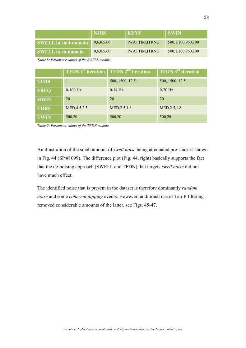
58
NOIS KEYS SWIN
SWELL in shot-domain 0,6,0.5,60 IWATTIM,ITRNO 500,1,100,960,100
SWELL in co-domain 0,6,0.5,60 IWATTIM,ITRNO 500,1,100,960,100
Table 8: Parameter values of the SWELL module
TFDN 1st iteration TFDN 2nd iteration TFDN 3rd iteration
TIMR 1 500,,1500, 12.5 500,,1500, 12.5
FREQ 0-100 Hz 0-14 Hz 0-20 Hz
HWIN 20 20 20
THRS MED,4.5,2.5 MED,2.5,1.8 MED,2.5,1.8
TWIN 500,20 500,20 500,20
Table 9: Parameter values of the TFDN module
An illustration of the small amount of swell noise being attenuated pre-stack is shown
in Fig. 44 (SP #1099). The difference plot (Fig. 44, right) basically supports the fact
that the de-noising approach (SWELL and TFDN) that targets swell noise did not
have much effect.
The identified noise that is present in the dataset is therefore dominantly random
noise and some coherent dipping events. However, additional use of Tau-P filtering
removed considerable amounts of the latter, see Figs. 45-47.

59
Figure 44: From left to right: before, after and difference plots after SWELL and TFDN has been applied. This is the same SP as in the case of the scrapped line (Fig. 39).
Figure 45: The stacked section after designature and prior to any de-noising of the reference line. Box 1 and 2 indicate target areas that are going to be investigated further in section 5.3.

60
Figure 46: The stacked section after SWELL, TFDN and Tau-P filtering have been applied to the reference line. Amplitude gain has been applied.
Figure 47: The corresponding difference plot of the stacked section (before and after de-noising and Tau-P filtering).

61
After post-stack migration, the image shown in Fig. 48 is obtained. The migration
provides an improved image, and many of the dipping events have been efficiently
moved to their correct positions. Some coherent events have been unwrapped deeper
in the subsurface in this migrated section as well (7-8 s TWT). However, as already
indicated, they are assumed to be unwanted energy related to reverberations. Similar
diffraction curves can still be noticed in the shallow parts of this migrated section as
well and are most probably related to some wrong velocities. Migration artefacts
(smiles) can also be observed on both sides of the stacked section (encircled areas)
due to the shortening of the line (edge effects).
Figure 48: Post-stack migration of the reference line. Not any large visual differences when compared to the migrated section of the scrapped line (cf. Fig. 43). Same migration artefacts can be observed, especially from 4 s TWT (encircled areas). Amplitude gain has been applied.

62
5.3. Comparison of the scrapped line and the reference line This section discusses the results obtained for both lines in more detail. Sometimes it
may be difficult to see the visual differences on a stacked section. Thus, two target
areas (one shallow and one deeper) have been introduced earlier so that one can zoom
in to smaller selected parts of the stacked section. The idea is to compare these
zoomed areas both visually and by calculating the RMS values for the reference and
the scrapped line.
The calculated RMS noise (𝑅𝑀𝑆 ) values give an indication of the amount of noise
that has been removed from each dataset and reveals which output result is
supposedly best. The RMS results are presented in Tables 10 and 11 for the scrapped
line and the reference line respectively. As expected, the RMS input (𝑅𝑀𝑆 ) values
are generally higher for the scrapped line compared to the reference line. The RMS
results show, however, that the RMS output (𝑅𝑀𝑆 ) values of the scrapped line are
very similar to those of the reference line.
De-noising approach RMS (input) RMS (output) RMS (noise)
SWELL/TFDN/ TAUP (Box 1) 1.09 1.02 0.36 SWELL/ TFDN/ TAUP (Box 2) 1.16 0.55 1.02 Whole stacked section 2.35 0.98 2.14 Table 10: Calculated RMS values of the stacked section for the scrapped line (434060A-033), before and after applying the optimized de-noising combination and Tau-P filtering.
De-noising approach RMS (input) RMS (output) RMS (noise)
SWELL/TFDN/ TAUP (Box 1) 1.05 0.99 0.34 SWELL/TFDN/ TAUP (Box 2) 1.05 0.58 0.88 Whole stacked section 1.62 0.98 1.28 Table 11: Calculated RMS values of the stacked section for the reference line (434060B-048), before and after applying the optimized de-noising combination and Tau-P filtering.
Some minor differences can be observed with a slightly better 𝑅𝑀𝑆 values for Box 1
in case of the reference line and the opposite in case of Box 2. However, when taking
into account the complete stacked section, the 𝑅𝑀𝑆 is practically the same (0.98).
The conclusion based on the RMS values is therefore that after the optimized de-
noising combination and Tau-P filtering, the two lines are very similar in data quality.

63
The quantitative results represented by the RMS values in Tables 10 and 11 can also
be supported by direct visual inspection. Figures 49 and 50 show the results obtained
for the selected area represented by Box 1 for the scrapped line and the reference line
respectively. To furthermore ease the comparison, a smaller subset of stacked traces
(CDP range 1740-1750) has been magnified. Direct comparison between Figs. 49 and
50 show that the two results are indeed comparable.
Figure 49: Zoomed section of box 1 of the scrapped line after optimized de-noising combination and Tau-P filtering have been applied (left) and a small selected section of CDP´s (traces 1740-1750) to the right.
Figure 50: Zoomed section of box 1 of the reference line after optimized de-noising combination and Tau-P filtering have been applied (left) and a small selected section of CDP´s (traces 1740-1750) to the right.

64
Figure 51 shows the average spectrum of the small subset of stacked traces introduced
in the previous two figures. The spectral content is very similar within the frequency
band for the scrapped and the reference data. In order to provide a complete picture,
the same averaged spectra are shown in Fig 52 before any de-noising. One may
observe that some differences exist for the very low frequencies (0-5 Hz), see
encircled areas (Fig. 52).
Figure 52: Average amplitude spectra of the selected traces 1740-1750 in box 1 of the scrapped line (black) and the reference line (red) before de-noising has been applied.
Figure 51: The average spectrum of the selected traces 1740-1750 in box 1 of the scrapped line (black) and the reference line (red) after the optimized de-noising combination and Tau-P filtering.

65
The final image of Box 1 of the scrapped and the reference data are shown in Fig. 53.
Again, the datasets appear very similar. However, note a dipping event in the
scrapped data that has been better preserved than the reference data.
Figures 54-57 show the same results as those given by Figs. 49-52, the only
difference being that the target area has changed from Box 1 (shallow) to Box 2
(deeper). Again, visual inspection shows that after optimal processing the scrapped
line and the reference line look very similar within this area. Not any significant
differences after direct comparison between Figs. 54 and 55. The averaged spectra
also confirm this, see Fig. 56. Again in order to provide the complete picture, the
averaged spectra are also shown before de-noising has been applied (cf. Fig. 57).
Direct comparison between Figs. 56 and 57 demonstrates that the de-noising of the
scrapped line has worked well (compare encircled area). Random noise has also
efficiently been removed from both the scrapped and the reference line by comparing
the amplitude level for higher frequencies.
Figure 53: Migrated section of the scrapped line (Box 1) to the left. Migrated section of the reference line (Box 1) to the right.

66
Figure 55: Zoomed section of box 2 of the reference line after optimized de-noising combination and Tau-P filtering have been applied (left) and a small section of CDP´s (traces 2870-2880) to the right.
Figure 54: Zoomed section of box 2 of the scrapped line after optimized de-noising combination and Tau-P filtering have been applied (left) and a small section of CDP´s (traces 2870-2880) to the right.

67
Figure 57: The average spectrum of the selected traces 2870-2880 in box 2 of the scrapped line (black) and the reference line (red) before de-noising has been applied.
Figure 56: The average spectrum of the selected traces 2870-2880 in box 2 of the scrapped line (black) and the reference line (red) after optimized de-noising combination and Tau-P filtering.

68
The final results after migration, within the deeper parts of the section (Box 2) of the
scrapped and the reference data are shown in Fig. 58. No significant visual differences
can be seen. However, some reflectors may appear a bit stronger in favour of the
reference line, see encircled areas (Fig. 58). Nevertheless, the general results obtained
after visual inspection of Box 1 and 2 are consistent with the calculated RMS values.
The amplitude spectrum for the whole stacked section before and after the optimized
de-noising combination and Tau-P filtering respectively is shown in Figs. 59 and 60.
The black curve represents the scrapped data and the red curve represents the
reference data. The encircled area emphasizes the abnormal high amplitudes of swell
noise that corrupts the scrapped dataset (Fig. 59). Again, these amplitudes are
successfully damped after the optimized de-noising combination and Tau-P filtering
have been applied (Fig. 60). This supports the overall similarity between these two
datasets that has been indicated earlier. It also demonstrates that the overall quality of
the whole stacked section, and not only small sections, has been improved.
Figure 58: Migrated section of the scrapped line (Box 2) to the left. To the right, the migrated section of the reference line (Box 2)

69
Figure 60: Amplitude spectrum of the whole stacked section (4301 traces) after the optimized de-noising combination and Tau-P filtering. The black curve represents the scrapped line and the red curve represents the reference line.
Figure 59: Amplitude spectrum of the whole stacked section (4301 traces) before de-noising. The black curve represents the scrapped line and the red curve represents the reference line. The encircled area emphasizes the high amplitude swell noise of low frequencies that is corrupting especially the scrapped dataset.

70
The magnitudes of the amplitude response of the scrapped line and the reference line
are given in Table 12 and 13 respectively. They summarize the differences before and
after the optimized de-noising combination and Tau-P filtering for the frequencies in
the range of 1-6 Hz. These quantified results are given for Box 1 (cf. Figs. 51 and 52),
Box 2 (cf. Figs. 56 and 57) and for the whole stacked section (cf. Figs. 59 and 60).
Table 12: The amplitude spectrum values (in dB) of the scrapped line (before and after de-noising)
Table 13: The amplitude spectrum values (in dB) of the reference line (before and after de-noising)
Line 033 Box 1 Box 2 Whole stacked section FREQ Before de-
noising After de-noising
Before de-noising
After de-noising
Before de-noising
After de-noising
1 Hz -26.51 -28.95 -16.66 -27.00 -21.23 -24.76 2 Hz -22.70 -28.06 -8.32 -25.34 -6.72 -22.70 3 Hz -19.13 -26.51 -3.65 -33.19 -0.57 -18.28 4 Hz -17.38 -24.63 -2.81 -16.17 -0.40 -16.00 5 Hz -7.96 -9.08 -0.16 -2.18 -3.32 -7.34 6 Hz -25.36 -21.93 -12.34 -14.85 -12.09 -14.50
Line 048 Box 1 Box 2 Whole stacked section FREQ Before de-
noising After de-noising
Before de-noising
After de-noising
Before de-noising
After de-noising
1 Hz -26.50 -28.11 -31.70 -31.54 -35.58 -25.61 2 Hz -25.50 -26.58 -27.97 -32.22 -29.80 -23.65 3 Hz -26.93 -27.73 -21.33 -33.66 -21.57 -22.58 4 Hz -24.06 -22.01 -18.04 -27.13 -16.86 -18.33 5 Hz -10.52 -10.87 -3.10 -3.14 -14.90 -8.38 6 Hz -22.79 -21.21 -12.44 -13.15 -12.09 -14.83

71
6. Discussion
In this thesis, four de-noising modules have been tested in order to find an optimal de-
noising flow. Accordingly, the majority of the processing part has actually been
focused upon parameter settings, running jobs and QC of the output results. After
extensive testing, the optimized de-noising flow turned out to be a de-noising
combination between SWELL and TFDN. This de-noising combination was mainly
employed to attack the low frequency swell noise with abnormal high amplitudes but
also random noise. Significant amounts of swell noise were removed. Employing
Tau-P resulted in more significant attenuation of the random noise in addition to some
dipping events. These three modules removed the majority of the noise present in the
scrapped line, while the use of Tau-P was the most efficient one for the reference line.
The comparison of the output results of these two datasets should ideally give some
indication of how well the de-noising tools have worked. It turned out to be quite
different results after the optimized de-noising combination was applied pre-stack.
The last three shot gathers (SP #1097-1099) for both the scrapped line and the
reference line were investigated a bit closer. Large amounts of swell noise were
attenuated in the scrapped data, while the optimized de-noising combination
practically did not have any effect on the reference data.
The motivation for the use of Tau-P and migration was to investigate if some
primaries could be unmasked in the deeper section (5-8 s TWT). The crystalline
basement or geological structural features would have been important reference points
at such depths. Unfortunately, no primary reflections could be observed deeper than
3-4 s TWT. A brute stack provided by FMCS also supported this. In this case, the
most important results are based upon where it has been possible to recognize some
coherent events and inspect how well the noise has been attenuated in these areas.
Considering the comparison of the amplitude spectra, there are some larger local
variations before de-noising, especially in the range between 0-5 Hz. After the
optimized de-noising combination and Tau-P filtering, the amplitudes of the scrapped
line look more behaved and correlated to the reference line. The visual inspection and
the amplitude spectra show that the lines actually appear to be very similar, especially

72
considering Box 1 and for the whole stacked section. There are some larger local
variations up to 4 Hz in Box 2 (cf. Table 12 and 13), but overall, the results indicate
quite similar datasets.
The calculated RMS values are also indicating similar datasets with 𝑅𝑀𝑆 values of
0.98. This supports the fact that there is a strong correlation between these two
datasets after running the optimized de-noising combination and Tau-P filtering.
However, some reflectors or parts of the migrated stacked section of the reference line
can be considered to be of better visual quality than the scrapped line. These reflectors
are emphasized in Box 2 (cf. Fig. 58). Yet again, these differences are considered to
be minor and are most probably directly related to the survey when the data was
acquired, e.g. feathering effects. It would for instance never be possible to achieve the
same results from two different surveys, even if they happen to be in acquired in the
same area.
Within the target area in the shallow part (Box 1) there are only minor or insignificant
visual differences. This is quite natural since the deeper parts are typically more
affected by the high amplitude swell noise than the shallow parts. However, one
reflector stands out and appears stronger in the scrapped dataset (cf. Fig. 53).
Considering the whole stacked section, there are overall only minor differences. A
discussion on whether the scrapped line or the reference line is of better quality must
be based on where the actual target zone is.
In this thesis, two target zones have been investigated closer with successful results.
However, in order for these results to be more representative, future work within this
topic should include a well-defined target area (basement or other important structures
in the subsurface). A comparison with the finished product (the final processed
reference line) should also be considered. Furthermore, it would be suggested to run a
de-multiple job in order to remove the reverberations. It would provide a more
credible comparison. We also believe that more testing could have contributed to an
improved final result. Nevertheless, based on the overall results, it is possible to argue
that the seismic image obtained after processing of the scrapped line is similar to the
image obtained after processing of the reference line.

73
Regarding the new module that was tested, MINC, more testing would be
recommended. Some artefacts were observed above the sea floor event. However,
these could have been avoided if the filter would have been set to start below the
move-out of the sea floor. Due to the limited time frame of this thesis, there was no
possibility for testing this. Further suggestions could include testing MINC in some of
the other domains (CO domain and/ or CDP domain) in order to see how it performs.

74
7. Conclusions
The optimized de-noising approach (SWELL and TFDN) and additional use of Tau-P
have proven to be an efficient de-noising flow for the scrapped line (434060A-033)
and the reference line (434060B-048). Based on the quantified results and visual
inspection, the seismic lines appear to be very similar. They have the same frequency
content and it is difficult to claim that one of the datasets is of significant better
quality than the other.
The overall conclusion is that the applied de-noising techniques have been robust
enough to successfully attenuate the noise in a discarded dataset. The results also
provide arguments for accepting more noise in seismic data in the future. In addition,
the results suggest that the noise threshold of 15-20 𝜇𝐵𝑎𝑟, which has been the
standard for more than two decades, may be too conservative and might require some
reconsideration and adjustment. As the noise threshold was measured to be 27.5 𝜇𝐵𝑎𝑟
when the scrapped line was aborted, a new noise threshold value close up to this value
is suggested.
It may also be of interest from a commercial point of view, to be able to acquire data
in rougher weather. A higher noise threshold value may be a factor that can reduce
weather-induced delays associated with marine surveys.

75
References
Ashton, C. P., Bacon, B., Déplanté, C., Dickilreson, T. S. and Redekop, G. 1994. 3D
Seismic Survey Design. Oilfield Review, pp. 19-32.
Ashcroft, W. 2011. A Petroleum Geologist´s Guide To Seismic Reflection. Wiley,
John & Sons, Incorporated.
Bekara, M. and Van Der Baan, M. 2009. Random And Coherent Noise Attenuation By
Empirical Mode. Geophysics, Vol. 74; NO. 5, pp. 89-98.
Brown, A. R. 2004. Interpretation Of Three-Dimentional Seismic Data, 6th edition.
AAPG Memoir 42 and SEG Investigation In Geophysics, NO. 9, 542p.
Canales, L. L. 1984. Random noise reduction. SEG Technical Program Expanded
Abstracts, Vol. 3; NO. 1, pp. 525-527.
Elboth, T. 2010. Noise in Marine Seismic Data. A dissertation for the degree of
Philosophiae Doctor at the Faculty of Mathematics and Natural Sciences,
University of Oslo, 2010.
Elboth, T. and Hermansen, D. 2009a. Attenuation of noise in marine seismic data.
SEG Technical Program Expanded Abstracts, 28; NO. 1, pp. 3312-3316.
Elboth, T., Pettersson, B. A. R. and Andreassen, Ø. 2009a. Flow and swell noise in
marine seismic data. Geophysics, Vol. 74; NO. 2, pp. Q17-Q25.
Elboth, T., Presterud, I. V. and Hermansen, D. 2010. Time-frequency seismic data de-
noising. EAGE Geophysical Prospecting, Vol. 58; NO. 3, pp. 441-453.
Elboth, T., Qaisrani, H., and Hertweck, T. 2008. De-noising seismic data in the time-
frequency domain. SEG Technical Program Expanded Abstracts, Vol. 27; NO.
1, pp. 2622-2626.
Faleide, J. I., Bjørlykke, K., Gabrielsen, R.H : “Geology of the Norwegian
Continenetal Shelf” in: Bjørlykke, K. (Ed): Petroleum Geoscience: From
Sedimentary Environment to Rock Physics, 2010. pp. 467-499.

76
Fletcher, R. 2009. 2D Marine Processing Using Uniseis. Fugro Seismic Imaging Pty
Ltd. West Perth, Western Australia.
Fugro internal training notes. 2012.
Galbraith, M. 1991. Random Noise Attenuation By F-X Prediction: A Tutorial. 61st
Annual International Meeting, SEG, Expanded Abstacts, pp. 1428-1431.
Gelius, L. J. and Johansen, T. A. 2010. Petroleum Geophysics. UniGEO AS, Bergen
GoogleEarthTM. 2012. GoogleEarth. [Accessed 03.04. 2012]. Available at
http://earth.google.com/
Hardy, R.J.J. 2010. [Accessed 20.04. 2012]. Available at
http://www.xsgeo.com/course/basic.htm#tp
Hayes, M. H. 1996. Statistical Digital Signal Processing And Modeling. John Wiley
& Sons, Inc. United States of America.
Kearey, P., Brooks, M. and Hill, I. 2002. An introduction to Geophysical Exploration,
3rd edition. Wiley-Blackwell Science Ltd.
Olhovich, V. A. 1964. The Causes of Noise in Seismic Reflection and Refraction
Work. Geophysics, Vol. XXIX, NO. 6, pp. 1015-1030.
Presterud, I.V. 2009. Time frequency de-noising of seismic data: Master thesis at
Department of Geosciences, University of Oslo, 2009.
Rastogi, R., Yerneni, S. and Phadke, S. 2000. Aperture width selection criterion in
Kirchhoff migration. Association of Exploration Geophysicist Seminar on
Exploration Geophysics. Goa, India.
Sanchis, C. 2010. Signal Processing Techniques for the Enhancement of Marine
Seismic Data. A dissertation for the degree of Philosophiae Doctor at the
Faculty of Science Department of Physics and Technology, University of
Tromsø, 2010.

77
Sanchis, C., and Hanssen, A. 2011. Multiple-Input Adaptive Noise Canceller For The
Attenuation Of Non-Stationary Coherent Noise. Geophysics, Vol. 76; NO. 6, pp.
V139 – V150.
Smith, J. G. 1999. Amplitude and phase effects of weather noise. SEG Technical
Program Expanded Abstracts, Vol. 18; NO. 1, pp. 1485 – 1488.
So, H. C. and Leung, C. T. 2005. A Simple Improvement To Tufts-Kumaresan Method
For Multiple Sinusoidal Frequency Estimation. IEICE Transactions
Fundamentals, Vol. 88; NO.1, pp. 381-383.
Stein, S and Wysession, M. 2003. An introduction to seismology, earthquakes and
earth structure. Wiley-Blackwell.
Tufts, D.W. and Kumaresan, R. 1982. Estimation Of Frequencies Of Multiple
Sinusoids: Making Linear Prediction Perform Like Maximum Likelihood.
Proceedings of IEEE, Vol. 70; NO. 9, pp. 975-985.
Yilmaz, Ö. 2001. Seismic Data Analysis Volume 1. SEG, 2001.

78
Appendix A: Time domain VS frequency domain Any periodic waveforms, no matter how complex they might be, are made up by a
combination of cosine waves (Kearey, 2002). This is a theory proven by the
mathematician Jean Baptiste Joseph Fourier. This decomposition process is called
Fourier transform and makes it possible to go from one domain (acquisition) to
another domain (Fourier). Since the seismic data is recorded in the time domain, it
implies going from time domain to frequency domain. In the frequency domain the
sinusoidal waves can be visualized by their amplitude, frequency and phase shift,
rather than as monochromatic time signals (cosine functions). Each cosine function is
characterized by its length (amplitude) and the direction or displacement relative to
t=0 (phase). By adding all these cosine functions, the original time signal can be
obtained (inverse Fourier Transform) (Gelius and Johansen, 2010).
The transformed time domain signal is equivalent to an amplitude spectrum (peak
amplitude against frequency) and a phase spectrum (phase shift against frequency) in
the frequency domain. In order to illustrate this, a Ricker wavelet is given as an
example of the transformation, Fig. A1. It illustrates how a simple time domain zero
phase wavelet (symmetric about t=0) is transformed into its frequency domain
components (amplitude and phase spectra). The minimum phase spectrum case is
illustrated in Fig. A2.
Figure A1: The illustration to the left representing the time response of a zero phase wavelet. The corresponding representation of the amplitude and phase response associated with a transient waveform (right).

79
Bandwidth can be defined as the range of frequencies that are present in the wavelet.
In general, as the signal becomes more restricted in the time domain, the
corresponding representation in the frequency domain would be an extension of the
bandwidth (Fig. A3). The complementary nature of a monochromatic signal in the
time domain would appear as a spike in the frequency domain (Fig. A3a). As the
transient waveform becomes shorter in the time domain, the associated bandwidth in
the frequency domain becomes wider (Fig. A3b,c). In a limiting case an infinitely
narrow spike waveform (also known as a Dirac delta function) with an infinite
bandwidth would be the most desirable wavelet (Fig. A3d). However, this is far from
being realistic and can only be obtained in theory. Fig. A3c would be a more typical
example of a wavelet that would be possible to achieve in practical terms (Ashcroft,
2011).
Figure A2: The illustration to the left representing the time response of a minimum phase wavelet. The illustration to the right represents the corresponding amplitude and phase response associated with a transient waveform.

80
Figure A3: Complementary nature of time- and frequency domain, zero phase wavelet case (Ashcroft, 2011).

81
Appendix B: Calculation of RMS values Let us assume that a recording can be considered as the sum of a signal component
(S) and a noise component (N). Let 𝐸 represent the mean of any discrete random
variable. By definition, the RMS level of any input dataset is given by Eq. B.1. The
output dataset obtained after processing is assumed to have a signal component only.
Its RMS is then defined by Eq. B3. The RMS of the attenuated noise is defined by Eq.
B.2.
𝑅𝑀𝑆 = 𝐸((𝑆 + 𝑁) ) (B.1)
𝑅𝑀𝑆 = 𝐸(𝑁 ) (B.2)
𝑅𝑀𝑆 = 𝐸(𝑆 ) (B.3)
Assuming that the noise is zero mean (𝐸(𝑁) = 0) and that signal and noise are
uncorrelated, we have:
𝑅𝑀𝑆 = 𝐸((𝑆 + 𝑁) ) = 𝐸(𝑆 + 2𝑆𝑁 + 𝑁 ) =𝐸(𝑆 ) + 2 ∙ 𝐸(𝑆) ∙ 𝐸(𝑁) + 𝐸(𝑁 ) = 𝐸(𝑆 ) + 𝐸(𝑁 ) (B.4)
In order to calculate 𝑅𝑀𝑆 , this last expression can be rewritten as:
𝑅𝑀𝑆 = 𝐸(𝑆 ) + 𝐸(𝑁 ) = 𝑅𝑀𝑆 + 𝑅𝑀𝑆 →
𝑅𝑀𝑆 = 𝑅𝑀𝑆 − 𝑅𝑀𝑆 (B.5)
MatLab was used to calculate the RMS values and the following explicit formulas
were used:
𝑅𝑀𝑆 = ∑ (𝑠(𝑘) + 𝑛(𝑘)) (B.6)
And for 𝑅𝑀𝑆 :
𝑅𝑀𝑆 = ∑ 𝑠(𝑘) (B.7)
where M is the total number of samples considered and 𝑠(𝑘) is the amplitude of the
𝑘 sample (𝑘 = 1,2,3, . . . , 𝑀).
82
Ideally, the 𝑅𝑀𝑆 values should provide a fairly good indication of how much noise
that has been attenuated. Higher 𝑅𝑀𝑆 values represent stronger attenuation of the
noise, and vice versa. However, if the de-noising methods accidently should attenuate
any energy from the wanted signal, it will result in lower 𝑅𝑀𝑆 values and hence a
𝑅𝑀𝑆 value that appears higher than it actually should be. Hence, it is important to be
critical to these values and keep in mind that the calculated 𝑅𝑀𝑆 values may not be
accurate in such cases.

83
Appendix C: Application of MINC and TFDN This appendix summarizes the results obtained when using a de-noising approach
consisting of a combination of MINC and TFDN.
C.1. Scrapped line Table C.1 shows the parameters applied for the MINC module (shot domain only).
MINC 1st iteration MINC 2nd iteration
STEP 0.00005,0.001,0.01 0.00005,0.001,0.01
NSWIN HOLD,IDIST,1500,2300,11272,11645 HOLD,IDIST, 1500,2300,11272,11645
IFTHR PER,0.25,0.16 VAL, 6.936568,0.9182808
FORDER 50 50
EPSSET AUTO AUTO
Table C.1: Parameter values for the MINC module (scrapped line).
Noise sequences are extracted from a spatial window in the input marine shot gather
in order to identify the same type of noise that is corrupting the dataset. In this way,
the noise is estimated, and then subtracted from the input trace to give an error value,
which forms the mean-square estimate of the seismic signal. The same noise
sequences were used for all the calls of MINC. The filter was not applied to data
blocks because better results were obtained when applying the filter to the whole
trace.
IFTHR represents the threshold values either given in percentages (PER) or as
instantaneous frequency values (VAL). Higher values correspond to stronger
attenuation. A noise file that is created during the processing indicates the threshold
frequency values that may be used for following applications of MINC.
Main results are summarized in Figs. C.1-C.5 and Table C.2.
Notice that some artefacts related to the processing have been created in the MINC
output, close to the water bottom, see difference plot (Fig. C.4). The origin of these
artefacts has to be investigated more closely in the future.

84
Figure C.2: Stacked section of the scrapped line before de-noising has been applied.
Figure C.1: From left to right: before, after and difference plots after SWELL and MINC have been applied.

85
Figure C.3: Stacked section after application of MINC, TFDN and Tau-P filtering. Note that amplitude gain has been applied to this stacked section.
Figure C.4: The corresponding difference plot between Fig. C.2 and Fig. C.3.

86
De-noising approach RMS (input) RMS (output) RMS (difference)
MINC/TFDN/ TAUP (Box 1) 1.09 1.03 0.35 MINC/ TFDN/ TAUP (Box 2) 1.16 0.55 1.03 Whole stacked section 2.35 0.98 2.14 Table C.2: Calculated RMS values of the stacked section for the scrapped line (434060A-033) applying a de-noising combination with MINC and TFDN.
Note that the calculated RMS values of the MINC and TFDN combination are
actually competitive compared to the optimized de-noising combination in case of
SWELL and TFDN. However, they are not considered to be representative due to
some coherent event attenuation and the artefacts that occurred at the seafloor during
the processing.
Figure C.5: Migrated section after MINC, TFDN and TAUP de-noising. Note that amplitude gain has been applied this stacked section.

87
C.2. Reference line A challenge that occurs when applying MINC to this dataset was the setting of the
parameter values, because the instantaneous frequencies were correlated to the
seismic signal. This makes it difficult to apply MINC without affecting coherent
events. Therefore, softer threshold percentage values had to be applied, and, only one
iteration of MINC (Table C.3). The corresponding RMS values have also been
calculated and can be found in Table C.4.
Some of the artefacts could have been avoided if the starting point of the filter had
been set from 500 ms and not been applied to the whole dataset. The artefacts were
mainly observed above the seabed.
The results obtained for the reference line are summarized in Figs. C.6-C.10.
MINC 1st iteration
STEP 0.00005,0.001,0.01
NSWIN HOLD,IDIST,1500,2300,11272,11645
IFTHR PER,0.16,0.10
FORDER 50
EPSSET AUTO
Table C.3: Parameter values for the MINC module (reference line).
Figure C.6: The corresponding SP #1099, as in Fig. C.1. From left to right: Before, after and difference plots after MINC and TFDN de-noising.

88
Figure C.8: Stacked section after MINC, TFDN and Tau-P filter have been applied. The same scaling has been applied, as in Fig. C.3.
Figure C.7: Stacked section of the reference line before de-noising has been applied.

89
Figure C.10: Migrated section after MINC and TFDN and Tau-P de-noising.
Figure C.9: The corresponding difference plot (before and after MINC, TFDN and Tau-P filtering).

90
De-noising approach RMS (input) RMS (output) RMS (difference)
MINC/TFDN/ TAUP (Box 1) 1.05 1.00 0.33 MINC/ TFDN/ TAUP (Box 2) 1.05 0.57 0.88 Whole stacked section 1.62 0.99 1.27 Table C.4: Calculated RMS values of the stacked section for the reference line (434060B-048) applying a de-noising combination with MINC and TFDN.