performance and design of composite beams with web openings

PERFORMANCE AND DESIGN OF

COMPOSITE BEAMS WITH WEB OPENINGS

by

Rex C. Donahey

David Darwin

A Report on Research Sponsored by

THE AMERICAN INSTITUTE OF STEEL CONSTRUCTION

Research Project

21 .82

UNIVERSITY OF KANSAS

LAWRENCE, KANSAS

April 1986

,0272~101

REPORT DOCUMENTATION I'· REPORT NO. 2. 3.. Recipi•nt's Accession No..

PAGE 4. TJtl• and S...btttte 5. Report O•te

Performance and Design of Composite Aoril 1986 Beams with Web Openings ..

7. Authot(s) a. Performina: Organization Rept.. No:

Rex C. Donahey and David Darwin SM Report No. 18 9. Performing Oraanization Nam• and Addr.ss 10. Project/Task/Work Unit No.

Structural Engineering and Materials Laboratory University of Kansas Center for Research, Inc. 11. Contract(C) or Grant(G) No.

2291 Irving Hill Drive, West Campus (C)

Lawrence, Kansas 66045 (G) 21.82 12. Sponsorinc Organization Nam• and Address 13. Type of Report & Period Covered

American Institute of Steel Construction 400 North Michigan Avenue Chi cage, Illinois 60611-4185 14.

15. Suppl•mentary Notes

115. Abstract {Umft 200 words)

Fifteen tests to failure were carried out on full scale composite beams with web openings. All beams had ribbed slabs using formed steel deck. Ribs were perpendicular to or parallel to the steel section. The effects of moment-shear ratio, partial com-posite construction, deck rib orientation, slab thickness, opening shape, opening eccentricity, and modification of the deck over the opening are studied. A strength mode: and three versions of a practical design technique are developed. The model and

! the design techniques are compared with all experimental work on composite beams with web openings. Serviceability criteria are developed.

The peak loads attained by composite beams with ribbed slabs at web openings are governed by the failure of the slab. Rib failure occurs in slabs with transverse ribs, while 1 ongi tudinal shear failure occurs in slabs with longitudinal ribs. As the number of shear connectors above the opening and between the opening and the support increases, the failure load increases. The failure of composite beams with ribbed slabs is, in general, ductile. First yield in the steel around the opening does not give an accurate indication of the section capacity. The strength model and the design techniques ac-curately predict the strength of composite beams at web openings for beams with solid or ribbed slabs.

17. Doeum•nt Analysis a. Descriptors

beams (supports), buildings, composite structures, concrete, deflections, formed steel deck, load factors, openings, resistance factors, ribbed slabs, steel, structural analysis, structural engineering, ultimate strength, web beams

b. ldentlflers/Open·Ended Tenns

e. COSATt F1eld/Graup

18. Availability Statement 19. Security Class (This Rlfport) 21. No. of ?agn

!Jnrl ~'"'if i F!ct

Release Unlimited · 20. Security CJass (This P.age)

Unclassified 22. Price

(SM ANSI-Z39.18} See InstrUctions on Reverse OPTtONAt.. FORM 272 (4-77) (Formerly NTI.s-35} Department of Commen::e

ii

ACKNOWLEDGEMENTS

This report is based on a thesis submitted by Rex C. Donahey to

the Department of Civil Engineering of the University of Kansas in

partial fulfillment of the requirements for the Ph.D. degree.

The research was supported by the American Institute of Steel

Construction under Research Project 21 .82.

Stud welding equipment and shear studs were provided by the

Nelson Stud Welding Division of TRW. Steel decking was provided by

United Steel Deck, Inc. Reinforcing steel was provided by ARMCO INC.

and Sheffield Steel. Numerical calculations were performed at the

University of Kansas Computer Aided Engineering Laboratory.

iii

TABLE OF CONTENTS

Page

ABSTRACT .•.......••.••..... , • , ........•.•.• , . • . . . . . • . . • . . • . . i

ACKNOWLEDGMENTS. . . . • • • . . • . • • • . • • • . • • • • • • • . . • • • • . . • . • • . . • . . . • ii

LIST OF TABLES.............................................. vi

LIST OF FIGURES............................................. viii

CHAPTER 1 INTRODUCTION •...•...••........•.•••.••••.•.•••••

1 • 1 GENERAL ..............•.•........•.•......•..

1. 2 PREVIOUS WORK............................... 2

1. 3 OBJECT AND SCOPE............................ 9

CHAPTER 2 EXPERIMENTAL WORK............................... 10

2 . 1 GENERAL. • • • . • • . • . • . . . . . . • . . . . . . . . • • • . • • . • • . . 1 0

2. 2 TEST SPECIMENS.............................. 10

2.3 BEAM DESIGN................................. 13

2. 4 MATERIALS................................... 14

2.5 BEAM FABRICATION............................ 15

2.6 INSTRUMENTATION............................. 17

2.7 LOAD SYSTEM................................. 19

2.8 LOADING PROCEDURE........................... 20

CHAPTER 3 EXPERIMENTAL RESULTS............................ 22

3. 1 GENERAL... . . . • • . • . • . • . • . • . • • • . • . • • . . • • • • • • • • 22

3.2 BEHAVIOR UNDER LOAD ....... ,................ 23

3.3 DISCUSSION OF BEHAVIOR...................... 26

3.4 SUMMARY..................................... 29

iv

TABLE OF CONTENTS (continued)

Page

CHAPTER 4 STRENGTH MODEL.................................. 31

4. 1 GENERAL ••.••••••••••••••••••• , • • • • . • • • • • • • • • 31

4. 2 OVERVIEW OF THE MODEL... • .. .. .. .. • • . • • • .. • .. 32

4.3 MATERIALS................................... 35

4. 4 BOTTOM TEE. • . . . • • • . • . • • • • . • • • • • • • • • • • • • • • . • • 37

4.5 TOP TEE..................................... 47

4.6 DETAILS OF INTERACTION PROCEDURE............ 60

4. 7 COMPARISON WITH TEST RESULTS................ 62

CHAPTER 5 STRENGTH DESIGN PROCEDURES...................... 66

5. 1 GENERAL..................................... 66

5.2 OVERVIEW OF DESIGN PROCEDURES............... 69

5. 3 INTERACTION CURVE. • • • • • • • • • • • • • • • • • • • • • • • • • • 70

5.4 MAXIMUM MOMENT CAPACITY..................... 71

5. 5 MAXIMUM SHEAR CAPACITY.. .. • .. .. .. .. .. .. .. .. • 77

5.6 COMPARISON WITH TEST RESULTS................ 98

5. 7 RECOMMENDATIONS. • . . . • • • • • • • • • • • • • • • • • • • • • • • • 103

CHAPTER 6 DESIGN OF COMPOSITE BEAMS WITH WEB OPENINGS..... 104

6.1 GENERAL..................................... 104

6. 2 STRENGTH DESIGN. • • • • • • • • • • • • • • • • • • • • • • • • . • • • 104

6. 3 DETAILING..... . • • • • • • • • • • • . • • • • • • • • • • • • • . • • • 108

6. 4 DEFLECT ION. • • • • • . . • . • • • • • • • • • • . • • • • • • • • • • • • • 1 09

6.5 DESIGN EXAMPLE.............................. 111

6.6 SUMMARY..................................... 128

v

TABLE OF CONTENTS (continued)

Page

CHAPTER 7 SUMMARY AND CONCLUSIONS......................... 129

7.1 SUMMARY..................................... 129

7. 2 CONCLUSIONS... • • • • • • • • • • • • • • • • • • • • • • • • • • • . • • 129

7. 3 FUTURE WORK. • • • • • • • • • • • • • . • • • • • • • • • • • • • • • • • • 1 31

REFERENCES.. • • • • • • • • • . . • • • • • • . • • • • • • • • • • • • • • • • . • • • • • • • • • • • . • 133

TABLES •••.•••.•••••••..•••••.. ,............................. 138

FIGURES. • • • • • • • • • • • • • • • • • • . • • • • • • • . • . • . • • • • • . • • • • • • • • . • • . • • • 1 49

APPENDIX A NOTATION......................................... 216

APPENDIX B SUMMARY OF PREVIOUS EXPERIMENTAL WORK............ 224

APPENDIX C DETERMINATION OF NEUTRAL AXES

LOCATIONS IN THE BOTTOM TEE..................... 229

C.1 NEUTRAL AXIS IN THE FLANGE AT THE LOW

MOMENT END •••••••.••••••• , • . • • • • • • • • • • • • • • • • 229

C.2 NEUTRAL AXIS IN THE WEB AT THE LOW

MOMENT END ..••••••••••••••.••••••••••• , , • . • • 231

APPENDIX D MECHANISM SHEAR CAPACITIES OF TOP AND BOTTOM

TEES FOR COMPARISON WITH TEST DATA.............. 234

APPENDIX E DEFLECTIONS. • • • • • • • • • • • • • • • • • • • • • • • • • • • . • • • • • • • • 236

E. 1 GENERAL..................................... 236

E.2 ANALYSIS PROCEDURE.......................... 239

E. 3 MODELING ASSUMPTIONS........................ 244

E. 4 PARAMETRIC STUDY........... .. .. .. .. .. .. .. .. • 246

E. 5 RECOMMENDATIONS.. • . • . • • . • • • .. • • • .. • . • .. .. .. • 255

vi

LIST OF TABLES

Table No. Page

2.1 Steel Strength................................... 138

2.2 Concrete Properties.............................. 139

2.3 Section and Opening Dimensions................... 140

2.4 Stud and Rib Properties.......................... 141

3.1 TestBehavior.................................... 142

3.2 Test Results..................................... 143

3.3 Relative Deflection at Failure................... 144

4. 1 Ratios of Test to Calculated Strength for

the Strength Model............................... 145

5.1 Ratios of Test to Calculated Strength for

the Redwood and Poumbouras Procedure (33),

the Strength Model (Chapter 4),

and Strength Design Methods I, II, and III....... 146

5.2 Ratios of Test to Calculated Strength for

the Redwood and Poumbouras Procedure (33)........ 148

B. 1 Material Strengths for Previous Investigations ... 225

8.2 Section and Opening Dimensions for Previous

Investigations................................... 226

B.3 Stud and Rib Properties for

Previous Investigations .....•...............•....

8.4 Test Results for Previous Investigations ........ .

E. 1 Measured and Calculated Deflections

227

228

at 30 Percent of Ultimate Load................... 256

vii

LIST OF TABLES (continued)

Table No. Page

E.2 Measured and Calculated Deflections

at 60 Percent of Ultimate Load................... 257

E.3 Ratios of Deflection across the Opening to

the Deflection at the Point of Maximum Moment.... 258

E.4 Effect of a 12-3/8 x 24-3/4 in. Web Opening on

the Deflection of a W21 x 44 Composite Beam...... 259

xiv

LIST OF FIGURES (continued)

Figure No. Page

E.6 Calculated versus Measured Total Deflection

at 60 Percent of Ultimate Load. (a) Model V.

(b) Model NV..................................... 265

E. 7 Calculated versus Measured Deflection

across the Opening at 30 Percent of Ultimate

Load. (a) Model V. (b) Model NV.................. 266

E.8 Calculated versus Measured Deflection

across the Opening at 60 Percent of Ultimate

Load. (a) Model V. (b) Model NV.................. 267

3

increased above a predetermined value, the bottom tee is also as

signed increasing increments of shear. In a comparison with the

experimental results of Granade, the model greatly underestimates the

shear strength of composite beams with web openings (Fig. 1.1). The

model does, however, illustrate the significant increase in moment

capacity provided by the concrete.

Swartz and Eliufoo (40) developed an elastic analysis technique

for web openings in composite beams using the Vierendeel method.

Their technique is based on full composite action and considers a

transformed, cracked section. Their method compares reasonably well

with finite element solutions. Although Swartz and Eliufoo did not

make a comparison with experimental results, their test case uses the

same section and loading as Beam 2 in an experimental study by

Clawson and Darwin (9, 11). Comparison of Swartz and Eliufoos•

predictions with the experimental results indicates that the most

significant deviation is in the prediction of concrete stresses.

This deviation is probably due to their assumption of zero slip at

the concrete-steel interface.

Clawson and Darwin (9, 10, 11) conducted an experimental inves

tigation of composite beams with web openings and developed a

strength model to predict the behavior of the beams. Six openings

were tested with heights and lengths of 60 and 120 percent of the

steel section depth, respectively. All beams were constructed with

solid slabs.

4

They found that, although the peak loads were governed by

failure of the concrete slab, failure was generally ductile. They

also found that the compressive strains in the concrete generally

remained low, well after the steel had begun to yield. Prior to

failure, large slips occurred between the concrete and steel.

Clawson and Darwin observed that the moment to shear ratio

(M/V) at the opening had a prominent effect on the failure mode. For

openings under high bending stress and low shear, failure tended to

be governed by crushing of the concrete, while beams under moderate

or high shear exhibited Vierendeel action, with large differential

deformation through the opening. They also found that the point of

inflection in the portion of the beam above the opening, or top tee,

was not at the centerline of the opening, but was displaced towards

the low moment end.

Clawson and Darwin (10, 11) proposed a model in which the slab

contributes to both the moment and shear capacity at a web opening.

Shear forces are assigned both to the concrete slab and to the steel

tees. Concrete forces are assumed to exist only at the high moment

end of the opening, while the reinforcing steel is considered to be

yielding in tension at the low moment end of the opening.

The model developed by Clawson and Darwin accounts for combined

shear and normal stress in the concrete. A failure criterion for the

concrete was developed by transforming principal stress data (23) to

a state of combined shear and compression. Shear stresses in the

concrete are assumed to be effective over a width of the slab equal

5

to three times the slab thickness. The concrete force is limited by

the material model or by normal force equilibrium. Interaction

diagrams are generated by assigning increasing amounts of shear to

both the top and bottom tees. Clawson and Darwin show that the model

is conservative for beams with solid slab construction.

A simplified version of the model (11) was developed for use in

design. Maximum moment capacity and maximum shear capacity are

calculated for the beam at the opening, the values are plotted on a

moment-shear interaction diagram, and the points are connected with

an ellipse. The simplified version shows good agreement with the

detailed model (Fig. 1.2).

Cho (8) largely duplicated the work of Clawson and Darwin using

small sections relative to the concrete slab. He arrived at essen

tially the same conclusions.

More recently, Redwood and Wong (34, 46) conducted an ex

perimental and analytical study of composite beams with web openings.

They tested 6 rectangular openings with heights and lengths of 60 and

120 percent of the steel section depth, respectively. All beams had

ribbed slab construction with the ribs transverse to the steel

section.

Their work confirmed that the failure mode of composite beams

with web openings is largely a function of the M/V ratio. Beams with

high and medium M/V ratios had compressive failures of the concrete

slab, while beams with low M/V ratios had diagonal cracking above the

6

opening accompanied by rib splitting and separation of the steel and

slab.

The analysis procedure developed by Redwood and Wong (34)

obtains the maximum bending and shear strengths. The maximum moment

that can be sustained at the maximum shear is also calculated, gener

ating a vertical line on the right side of the interaction curve.

The curve is closed with an ellipse.

The procedure developed by Redwood and Wong is based on the

formation of four hinges, one at each corner of the opening. No

stress is allowed in the concrete at the low moment end, while the

concrete force at the high moment end of the opening is limited by

the shear capacity of the stud connectors above the opening. The

procedure is very conservative for high shear cases. Redwood and

Wong felt that it was important to model the compressive stresses in

the slab at the low moment end, brought about by slip of the concrete

deck, and that consideration of this should result in higher

predicted strengths.

Redwood and Wong expressed concern about concrete cracking at

working loads at the low moment end of openings subjected to high

shears (low M/V ratios). They did observe, however, that deflections

at working loads satisfied live load deflection criteria normally

used.

More recently, Redwood and Poumbouras (30, 32) tested three

additional openings. The tests were designed to study the influence

of the amount of shear connection above the opening and the effect of

7

construction loads acting on the steel section before composite

action is effective. The openings were subjected to high shears and

had a relatively low number of shear connectors between the opening

and the point of zero moment.

Redwood and Poumbouras concluded that limited shear connection

above the opening will significantly reduce the strength of openings

with low M/V ratios. They also concluded that construction loads up

to 60 percent of the non-composite beam strength at the opening have

only a small effect on the strength of the composite section.

Poumbouras (30) has proposed a strength model for composite

beams with ribbed slabs. Compressive forces are assumed in the slab

at both the low moment and high moment ends of the opening. The

concrete force at the low moment end is assumed to be at the top of

the slab at zero shear; however, it is allowed to move to the bottom

of the slab as the shear at the opening is increased. The concrete

force at the high moment end is selected such that moment equilibrium

is satisfied at the opening. The model is not conservative for

openings with high shear and a low number of shear connectors above

the opening and between the opening and the support.

Redwood and Poumbouras developed an analysis procedure that

includes the compressive force in the concrete at the low moment end

of the opening (33). This force is set equal to the total shear

connector capacity between the opening and the point of zero moment.

The shape of their interaction curve (Fig. 1.3) is similar to that of

Redwood and Wong (33). Their procedure provides a good match with

8

their tests ( 30, 32) and those of Redwood and \~ong (34, 46). They

do, however, express some concern about applying the theory to ope

nings with a heavy steel section and a thin slab.

Momeni (28) modified the model developed by Clawson and Darwin

to include web reinforcement in the analysis. His model allows the

cracked portion of the slab at the high moment end of the opening to

carry shear. A concrete material model described by a single func

tion is used in place of a two-function relationship used by Clawson

and Darwin (10, 11). The top tee is allowed to carry all of the

shear at the opening, up to the maximum shear capacity of the top

tee. The model produces unconservative results for beams using

shallow steel sections with openings with low M/V ratios.

Donoghue (15) proposed a design procedure that neglects the

shear contribution of the slab to strength. His procedure includes

consideration of web reinforcement at the opening.

The design procedure proposed by Redwood and Wong has been

incorporated in a design aid published by U.S. Steel (44). A series

of tables of non-dimensional parameters are presented to allow the

Fapid construction of interaction diagrams for composite beams with

web openings.

In a 1984 state-of-the-art paper, Darwin described the behavior

and failure modes of composite beams with web openings (14) and

summarized current analysis techniques.

Tests of prototype beams with reinforced openings were recently

conducted in Illinois (37) and in Australia (41). The former test

9

was conducted on a 2·1 in. deep beam with a large ( 15 x 39 in.) open

ing at the midspan. Failure occurred in the slab near the support.

The latter test was conducted on a 530 mm (20.9 in.) deep beam with a

large [300 x 715 mm (11.8 x 28.1 in.)] opening and a small [300 x 515

mm (11.8 x 20.3 in.)] opening at approximately the quarter points in

the span. The test was not continued to failure. The Australian

design was based in part on the Clawson and Darwin (10, 11) model and

on an elastic finite element analysis.

1.3 OBJECT AND SCOPE

This study consists of laboratory tests and detailed analyses

leading to a comprehensive design procedure for composite beams with

web openings.

Fifteen tests to failure were carried out on composite beams

with web openings. All specimens were full scale composite beams

with ribbed slabs using formed steel deck. Slabs had ribs oriented

either perpendicular to or parallel to the steel section. Parameters

investigated included moment-shear ratio, partial composite behavior,

deck rib orientation, slab thickness, opening shape, opening ec

centricity, and modification of the deck over the opening.

A strength model is developed which shows good agreement with

all experimental work on composite beams with web openings. Three

versions of a practical strength design technique are presented. A

comprehensive design procedure, including both strength and service

ability criteria is developed.

2.1 GENERAL

10

CHAPTER 2

EXPERIMENTAL WORK

A number of experimental investigations of composite beams with

rectangular web openings have been conducted (8, 9, 11, 19, 32, 34,

37, 41). Granade (19), Clawson and Darwin (9, 11), and Cho (8)

tested composite beams with solid, or flat-soffit slab construction.

Redwood and others at McGill University (32, 34, 46) tested composite

beams with ribbed slab construction with the ribs oriented transverse

to the steel section. Prototype tests were conducted in Illinois

(37) and Australia (41). The test configurations used in previous

investigations are summarized in Appendix B. This information is

used in Chapters 4 and 5 as input for strength calculations.

The current experimental study is designed both to investigate

parameters not included in earlier studies and to confirm trends

indicated in those studies.

2.2 TEST SPECIMENS

Nine test beams with a total of 15 rectangular web openings

were tested (Fig. 2.1 - 2.10). One W10 x 15 and eight W21 x 44

sections were used. All beams had ribbed slab construction; the

ribs were oriented transversely on 8 beams and longitudinally on 1

beam. All slabs were made using normal weight concrete. The con

crete slab dimensions, shear stud quantities and locations, and

opening sizes and locations were varied.

11

The moment-shear (M/V) ratio at the web opening has been shown

to have a significant effect on the behavior of composite beams with

web openings (9, 11). Tests 1 through 3 and and Test 6a were used to

provide additional information on the effect of the M/V ratio. Test

1 (Fig. 2.1) had a lowM/V ratio (3.5 ft.), Test 2 (Fig. 2.2) had a

medium M/V ratio (6.5 ft.), and Test 3 (Fig. 2.3) had a high M/V

ratio (45.1 ft.). For Test 6A (Fig. 2.5), the opening was placed at

a point of contraflexure (M/V = 0 ft.).

Tests 2, 4A, 4B, and 5A (Fig. 2.2 and 2.4), which had medium

M/V ratios (6.5 ft.), and Test 6B (Fig. 2.6), which had a low M/V

ratio (3.5 ft.) were used to investigate the effect of the quantity

of shear connectors above the web opening and between the opening and

the support. Tests 2 and 4B had a large number of shear connectors

between the web opening and the support, while Tests 4A and 5A had a

low number of shear connectors between the opening and the support.

Tests 2 and 5A had 4 and 2 shear connectors, respectively, above the

opening, while Tests 4A and 4B had none. The steel deck in Tests 4A

and 4B was attached to the steel beam at each rib above the opening

using puddle welds.

Test 6B (Fig. 2.6) was used to test a possible reinforcement

procedure for composite beams with web openings. 22 gage steel pans

were fabricated to match the deck profile (Fig. 2.11 and 2.12). The

pans were placed on the top flange of the steel beam between the ribs

of the deck from the high moment end of the opening to the support.

4 x 6 in. rectangular holes were cut in the deck above the pans and 2

12

shear connectors were welded through each pan to the steel beam.

During concrete placement, the concrete around the pans was well

consolidated to ensure that any voids were removed.

Most of the test openings were concentric (top and bottom steel

tees were of equal depth), had depths equal to 60 percent of the beam

depth (0.60d), and had lengths equal to 120 percent of the beam depth

(1 .20d). There were, however, exceptions. Test 5B (M/V = 6.5 ft.,

Fig. 2.4) had an opening with a 1 in. negative (downward) ec-

centricity and an opening shape of 0.67d x 1.20d. Test 8B (M/V =

2.46 ft., Fig. 2.9) had a 0.15 in. negative eccentricity and an

opening shape of o.63d x 1.84d. Test 9A (MIV = 3.5 ft., Fig. 2.10)

had a concentric opening and an opening shape of 0.71d x 1.20d. Test

9B (M/V = 3.0 ft., Fig. 2.10) had a 0.13 in. negative eccentricity

and an opening shape of 0.71d x 0.71d.

Tests 7A (M/V = 3.5 ft.) and 7B (M/V = 6.5 ft.) (Fig. 2.7) were

used to study the effect of deck orientation on composite beams with

web openings and used steel deck with the ribs placed parallel to the

beam.

Tests 8A (M/V = 3. 28 ft.), 8B, 9A, and 9B (Fig. 2.8 - 2.10)

were used to evaluate the effect of the relative thickness of the

slab on opening behavior. Tests 1 through 7B had relatively thin

slabs compared to the depth of the beam, while Tests SA through 9B

had relatively thick slabs. The ratio of the slab thickness above

the ribs, t , to steel beam depth, d, for Tests 1 through 7B was s

13

approximately 0.1. The ratios for Beams 8 and 9 were 0.25 and 0.19,

respectively.

2.3 BEAM DESIGN

The composite beams were designed following the AISC Steel

Construction Manual (2). All beams were designed to be fully com

posite and were designed to fail at the web opening.

The slab reinforcement for Beams 1 to 6, 8 and 9 was designed

following the ACI Building Code (1). Transverse and longitudinal

reinforcement were selected to meet ACI temperature steel require

ments based on the gross slab thickness. Reinforcement consisted of

#3 bars on nominal 12 in. centers in both directions and provided a

nominal slab reinforcement ratio of 0.0018. The longitudinal rein

forcement rested on the formed steel deck, and the transverse

reinforcement was tied to the longitudinal reinforcement at the

centerlines of the deck ribs. Beam 7 reinforcement was selected

based on Steel Deck Institute recommendations for minimum temperature

steel (36). The minimum recommended reinforcing ratio is 0.00075

based on the slab thickness above the deck flutes. 6 x 6-W1.4 x W1.4

welded wire fabric was placed at the top of the steel decking.

The metal decking was selected to minimize the decking stiff

ness and to minimize the net concrete above the deck. 22 gage

decking with 3 in. deep ribs on 12 in. centers was selected,

14

2.4 MATERIALS

Beams 1 through 6 were fabricated using A572 Grade 50 W21 x 44

sections. Beams 7 and 9 were fabricated using A36 W21 x 44 sections.

Beam 8 used an A36 W10 x 15 section. The yield strength, static

yield strength and tensile strength of the rolled sections were

measured using standard test coupons from both the web and the

flanges in a screw-type test machine. Specimens were loaded through

the yield plateau at a relative head speed of 0.5 mm/min. At a

minimum of two points on the yield plateau, the displacement was

stopped so that the static yield load could be determined. When the

load stabilized (at the static yield load), displacement was resumed.

When strain hardening was observed, the relative head speed was

increased to 5 mm/min. and loading was continued to failure. The

average steel properties are summarized in Table 2.1.

The deformed reinforcing steel was Grade 60 with a yield stress

of 70.9 ksi. The yield stress of the welded wire fabric was measured

as 90.9 ksi using the 0.2% offset method.

All shear studs were supplied by the Nelson Stud Welding

Division of TRW. Beams 1 through 7 had 3/4 in. diameter studs with a

tensile strength of 67.9 ksi. Beam 8 had 5/8 in. diameter studs with

a tensile strength of 63.2 ksi, and Beam 9 had 3/4 in. diameter studs

with a tensile strength of 68.8 ksi. The 3/4 in. diameter studs were

Nelson Type S3L, and the 5/8 in. diameter studs were Nelson Type H4L,

modified for through-deck welding.

15

The steel decking was 22 gage Lok-Floor decking with 3 inch

ribs supplied by United Steel Deck, Inc. The deck profile is shown

in Fig. 2.12. The yield and tensile strengths of the decking were

40.7 ksi and 53.1 ksi, respectively.

The concrete was normal weight, Portland cement concrete sup

plied by a local ready-mix company. Coarse aggregate was crushed

limestone, and fine aggregate was Kansas River sand. All mixes were

ordered with entrained air. Concrete slump and air content were

measured at the time of placement. Concrete strengths were measured

using standard 6 by 12 in. test cylinders. Concrete properties are

summarized in Table 2.2.

2.5 BEAM FABRICATION

The initial step in beam fabrication was the preparation of the

web opening. The opening location was marked and 3/4 in. diameter

holes were drilled at the corners to reduce stress concentrations.

The opening was flame cut using an oxy-acetylene torch. Strain gage

locations were ground with an abrasive wheel.

Stiffeners were either welded or bolted to the beam web at load

points and supports on Beams 2 through 9. No stiffeners were used on

Beam 1. Bearing plates for the beam supports were bolted in place.

The steel section was supported at each end, and shoring was

installed to support the deck. Metal decking was positioned on the

section and attached to the shoring with nails to prevent deck move

ment during stud welding. Shear studs were welded though the deck

16

using a Nelson Stud Welding unit. With the exception of Beam 4,

studs were welded in each rib. The ribs over the openings in Beam 4

were attached to the wide flange section using 3/4 in. puddle welds.

After the shear studs were welded in place, the deck was

scraped and brushed to remove welding debris. The nails holding the

decking to the shoring were removed and the form sides were

installed. All joints between the steel decking and concrete forms

were caulked, and the reinforcing steel was installed.

The concrete was delivered by truck and placed using a 1 cubic

yard bucket. After the forms were filled, the concrete was con

solidated using a 1-112 in. electric vibrator inserted on 1 ft.

centers. The concrete was screeded using a metal-edged screed and

finished using a magnesium bull-float.

Slump and air tests were performed and test cylinders were cast

as the beam was cast. After the concrete had begun to set, the slab

and the test cylinders were covered with polyethylene sheets. All

test cylinders were stored near the slab. The beam and the cylinders

were kept continuously moist until a strength of 3000 psi was

reached. The concrete was then allowed to dry.

Two openings were tested on Beams 4 through 9. After the first

opening was tested, a second opening was cut in the steel section at

the opposite end of the beam. A plate was welded in the first

opening. The damaged concrete above the first opening was repaired

using gypsum cement grout or high strength concrete.

17

On Tests 48, 58, and 68, transverse cracks formed in the slabs

above the openings when the openings were cut. On Tests 48 and 6B,

the cracks formed at the low moment edge of the rib peak at the low

moment end of the opening, while on Test 58, the crack formed at the

high moment edge of the rib peak at the high moment end of the

opening. All of the cracks extended completely across the top of the

slab and extended approximately 1 in. down the side of the slab.

The opening locations, load configurations, and span lengths

are shown in Fig. 2.1 through 2.10. Section and opening dimensions

are summarized in Table 2.3. Stud quantities and rib dimensions are

summarized in Table 2.4.

2.6 INSTRUMENTATION

The beams were instrumented with electrical resistance strain

gages and DC linear variable differential transformers (LVDT's).

Strain gages were placed on both the steel and the concrete around

the opening. Steel gages were located along a line 1-112 in. from

the vertical edges of the opening to reduce the effect of stress

concentrations at the opening corners. Concrete gages were placed on

the top of the slab for all tests. In most cases, concrete gages

were also placed on the bottom of the slab. 1 by 4 in. slots were

cut in the steel decking and closed with duct tape before concrete

placement. The tape was supported from below. Before the beam was

tested, the support and tape were removed to expose the bottom of the

slab.

18

Micromeasurements 120 ohm foil strain gages with a 0.240 in.

gage length were applied to the steel following the gage manufac

turer's recommended procedures. Precision Measurements 120 ohm

paper-backed strain gages with 2.4 in. gage lengths were bonded to

the concrete using Duco cement. All gages were wired with shielded

cables. For Tests 1 through 3, the strain gages were read using

Vishay Model P-350A strain indicators and a Hewlett-Packard 3052A

data acquisition system with Diego Systems Model 113 strain gage

conditioners. For Tests 4A through 98, strain gages were read using

a Hewlett-Packard Model 3054A data acquisition system. For all

beams, the data acquisition system was controlled using a Hewlett

Packard 9825T Computer.

LVDT's were installed at the point of maximum moment and at the

ends of the opening to monitor beam deflection, LVDT's were also

installed at the ends of the concrete slab to monitor slip between

the slab and the steel section.

Some of the openings had LVDT's installed at the ends of the

opening to monitor the relative movement of the slab and the steel

section. For these beams, steel bars were embedded in the slab to

allow the measurement of horizontal slip. Holes were also cut in the

steel decking to allow the vertical separation to be monitored. All

LVDT's were read using the Hewlett-Packard data acquisition systems.

White wash was applied to the steel beam around the web opening

to act as brittle coating. Diluted latex paint was applied to the

concrete slab so that cracks could be seen.

19

2.7 LOAD SYSTEM

When the concrete reached the desired strength, the deck shor

ing was removed, and the beam was placed on pin and roller supports.

Bearing plates were grouted to the concrete at the load points. On

beams with transverse deck ribs, additional bearing plates were

grouted between the steel beam and the steel deck (load was applied

at the rib peak). The loading system was installed (Fig. 2.13).

The loading system applied load at one or two load points on

each beam. At each load point, two tension rods transferred load

through rockers to the top of a transverse load beam in contact with

the test specimen. All load systems, with the exception of the load

system for Test 8B, had 1-1/2 in. diameter hot-rolled tension rods.

The load system for Test 8B had 1 in. diameter cold-rolled tension

rods. The tension rods extended through openings in the load beam,

the concrete slab, and the lab structural floor. Below the struc

tural floor, the rods passed through hollow core Enerpac jacks which

applied the load (Fig. 2.13). Hydraulic pressure was applied using

an Amsler pendulum dynamometer. A manifold with flow control valves

was used to control the individual jacks to prevent twisting of the

test beam.

The tension rods were instrumented as load cells using two

longitudinal and two transverse gages in a full-bridge circuit and

were calibrated using a Tinius-Olsen column tester. The tension rods

were monitored using a Hewlett-Packard data acquisition system and

20

computer. During a test, the load and deflection were monitored at

two second intervals.

For Beams 1 through 6, Test 8A, and Beam 9, the total weight of

the load system was 0.6 kips per load point. For Beam 7, which did

not require bearing plates between the steel beam and the steel deck,

the weight was 0.55 kips per load point. For Test 8B, which had

in. diameter tension rods, the weight was 0.44 kips per load point.

2.8 LOADING PROCEDURE

Each beam was cycled 13 times to low maximum loads to relieve

residual stresses, to seat the loading system, and to test the

instrumentation.

The tests to failure were run using the following procedure.

Initial readings were taken at zero hydraulic system pressure and

with the jacks hanging freely from the load rods. The first and

second load increments were equal to the peak load of the pre-test

cycles. The remaining load increments varied according to beam

behavior. Preselected increments of load were used until the load

deflection curve indicated the beam was softening (the load

deflection curve became nonlinear). Load increments were then

selected to produce increments of deflection for the remainder of the

test. Load and deflection were plotted continuously. Concrete

cracks were marked at each load step using felt pens. Prior to

softening, the load was maintained while the instrumentation was read

21

and cracks were marked. Once the load deflection curve became non

linear, the deflection was maintained while readings were taken and

cracks were marked. After failure, all additional cracks were marked

and photographs were taken.

Two of the 15 tests deviated from the standard loading proce

dure. During Tests 1 and 3, after the specimens had been loaded well

above their initial yield, the specimens had to be unloaded and then

reloaded to failure. For Test 1, significant twisting of the beam

was noted at 70 percent of the ultimate applied load. The beam was

unloaded and the load system was adjusted to compensate for the

twisting. For Test 3, large deflections at 98 percent of the ul

timate applied load caused large rotations in the load beams,

resulting in bending of the load rods. The beam was unloaded and the

load system was adjusted to compensate for the rotation of the load

beams. After the beam was reloaded to 98 percent of ultimate, the

beam had to be unloaded a second time for further adjustments prior

to the final application of load.

The results of the tests are described in the next chapter.

3.1 GENERAL

22

CHAPTER 3

EXPERIMENTAL RESULTS

Previous experimental work has shown that the deformation and

failure mode of composite beams with web openings is largely a func

tion of the moment-shear (M/V) ratio at the opening ( 8, 9, 11, 19,

32, 34, 36).

For openings with high M/V ratios, the openings tend to have

small relative deformations across the opening and to fail in a

flexural mode. At failure, the bottom tee completely yields in

tension, and the concrete crushes at the high moment end of the

opening.

As the M/V ratio decreases, the Vierendeel effect becomes more

pronounced, as the shear at the opening induces secondary bending

moments in the tees. Differential deflections across the opening

increase. The concrete tends to crack at the top of the slab at the

low moment end of the opening, and the bottom tee has compressive, as

well as tensile strains. At failure, the concrete slab tends to

separate from the steel section at the high moment end of the

opening. Beams with solid slabs display a diagonal tension failure

in the slab (9, 11), while beams with ribbed slabs display rib

separation cracking (34, 46).

The results of the tests from the current study are presented

and evaluated in the following sections.

23

3.2 BEHAVIOR UNDER LOAD

Most of the tests in the current study had relatively low M/V

ratios (Tests 1, 2, 4A-9B). For these tests, the behavior under load

was dominated by the effects of secondary bending. Large differen

tial deformations across the opening were observed as the beams were

loaded (Fig. 3.1). One test (Test 3) had a high M/V ratio. The

behavior of this opening was dominated by the primary moment at the

opening. Relatively small differential deformations across the

opening were observed (Fig. 3.2).

Load-deflection diagrams for the 15 tests in this study are

presented in Fig. 3.3 to 3.17. Strain distributions at the opening

are presented in Fig. 3.18 to 3.32 for 4 stages of applied load

(elastic, first yield, late yield, and collapse)~

As a general rule, the failure of the beams was quite ductile.

The peak loads were preceeded by major cracking in the concrete,

yielding of the steel, and large deflections in the member (Fig. 3.3

- 3.17).

In all cases, yielding in the steel tees was observed at rela

tively low levels of loading (Fig. 3.18-3.32). As the tests

progressed, transverse and longitudinal cracking occurred in the

slabs. As the tests approached ultimate, the concrete around the

shear studs above the opening failed, and the slab lifted from the

steel beam at the high moment end of the opening.

The applied load at first yield and the applied load at the

first occurrence of transverse, longitudinal, and diagonal cracking

24

near the opening are presented in Table 3.1. These loads are ex

pressed as percentages of the applied (total - dead) load at failure.

First yielding was noted in tension in the top or the bottom

tee. For Tests 1-6A, and 7A-8A, first yielding occurred in tension

at the top of the low moment end of the bottom tee. For Tests 6B,

8B, 9A, and 9B, first yielding occurred in tension at the bottom of

the high moment end of the top tee. First yielding occurred at

applied loads as low as 19 percent, and as high as 52 percent of

ultimate, with an average of 33 percent (Table 3. 1). As concluded

for beams with solid slabs (9, 10), the first yield does not give an

accurate measure of section capacity.

Transverse, diagonal, and longitudinal cracks were noted in the

slabs as the loads increased. Transverse cracks formed in the top of

the slab at the low moment end of the openings (Fig. 3.33). The

cracks occurred at applied loads as low as 25 percent, and as high 96

percent of ultimate (Table 3.1). For Tests 4B, 5B, and 6B,

transverse cracks occurred when the opening was being cut. However,

these cracks appeared to have no effect on the behavior of the open

ing under load. As the loading increased, all transverse cracks

increased in width and in depth, eventually propagating to within

approximately 1/2 in. of the bottom of the slab.

All tests with transverse ribs displayed diagonal cracking.

Diagonal cracking occurred at an average applied load of 63 percent

of ultimate. Diagonal cracks started at the high moment end of the

opening at the low moment end of a rib and propagated toward the load

25

point as the load was increased. For Tests 7A and 78, which had

longitudinal ribs, no diagonal cracks were observed.

Longitudinal cracking (Fig. 3.33) occurred at an average ap

plied load of 80 percent of ultimate. Longitudinal cracks started at

the top of the slab at the low moment end of the opening directly

above the steel section and propagated toward the load point and the

support as the load increased.

Failure at openings was preceeded by failure of the concrete

around the studs above the opening and between the opening and the

support. For the tests with longitudinal ribs, a longitudinal shear

failure occurred between the rib and the surrounding deck (Fig.

3.34), and a slight slab uplift was noted. For the tests with

transverse ribs, the concrete failed in a shearing mode in the rib

(Fig. 3.35). The rih pulled away from the concrete around the stud

group, leaving a wedge-shaped block. For high shear tests on beams

with ribs transverse to the steel section (Tests 1, 2, 4A-6A, and 8A-

98), rib failure was followed by slab uplift, resulting in bridging

of the slab over the opening (Fig. 3.36). For the high moment test

(Test 3), only a minor slab uplift was noted (Fig. 3.2). For tests

68, 8A, and 88, the diagonal cracks in the slab propagated to the top

surface of the slab near the load point. All tests exhibited a large

amount of slip between the concrete and steel.

At all stages of loading, strains at the opening indicate a

lack of strain compatibility between the tees and between the top tee

steel and the slab (Fig. 3.18-3.32). The strain data show that, with

26

the exception of Test 3 (high M/V) (Fig. 3.20), strains were quite

low in the concrete slab at failure.

The moments and shears at ultimate and the modes of failure for

the current test series are presented in Table 3.2. The failure

loads include the weight of the beam and load system, as well as the

applied loads.

3.3 DISCUSSION OF BEHAVIOR

The tests in the current study confirm that the behavior of

composite beams with web openings is largely controlled by the M/V

ratio at the opening. Deformation, cracking in the slab, and the

failure load are all functions of the M/V ratio.

In general, the deflection across a web opening, 6 , increases 0

as the M/V ratio decreases. It is useful to normalize 60

with

respect to the deflection at the point of maximum moment at failure,

om, to obtain a normalized opening deflection, 6 = 60

/om.

and o are summarized in Table 3.3.

For tests with low to intermediate M/V ratios, o is high. As

the M/V ratio increases, o decreases. Tests 1 through 6B had similar

sections. 6 was 2. 27 for Test 6A (M/V = 0), an average of 1. 06 for

Tests 1 and 6B (M/V = 3.5 ft), an average of 1.03 for Tests 2, 4A,

4B, SA, and 5B (M/V = 6.5 ft), and 0.03 for Test 3 (M/V = 45.2 ft).

Transverse cracking of the concrete slab at the low moment end

of the opening is also strongly affected by the M/V ratio. As the

M/V ratio decreases, transverse cracks tend to appear at lower loads.

27

Cracking occurred at only 21 percent of the maximum applied load for

Test 6A (M/V = 0), an average of 42 percent for Tests 1 and 7A {M/V

3.5 ft), an average of 65 percent for Tests 2, 4A, 5A, and 7B (M/V =

6.5 ft), and 96 percent of the maximum load for Test 3 (M/V = 45.2

ft) (Table 3.1).

Longitudinal and diagonal cracking of the slab appear not to be

functions of the M/V ratio (Table 3. 1). Longitudinal cracking oc

curred at 70 percent of the maximum applied load for Test 6A (M/V =

0), an average of 86 percent for Tests 1 and 7A (M/V = 3.5 ft), an

average of 84 percent for Tests 2, 4A, 5A, and 7B (M/V = 6.5 ft), and

76 percent for Test 3 {M/V = 45.2 ft). Diagonal cracking occurred at

70 percent of the maximum applied load for Test 6A, an average of 67

percent for Tests 1 and 7A, an average of 81 percent for Tests 2, 4A,

5A, and 7B, and 76 percent for Test 3.

The failure loads were affected by the quantity of shear con

nectors above the opening and between the opening and the support.

As the quantity of connectors increased, the failure load tended to

increase. Tests 2, 4A, 4B and 5A had M/V ratios of 6.5 ft, had the

same section and opening dimensions, and had approximately the same

material strengths. Test 2 had a high number of studs over the

opening and between the opening and the support (H-H), Test 4A had no

studs over the opening and a low number of studs between the opening

and the support (N-L), Test 4B had no studs over the opening and a

high number of studs between the opening and the support (N-H), and

Test 5A had a low number of studs above the opening and a low number

28

of studs between the opening and the support (L-L). The shears at

failure for Tests 2 (H-H), 48 (N-H), 5A (L-L), and 4A (N-L) were

39.0, 39.0, 34.6, and 32.7, respectively (Table 3.2).

Test 48 (N-H) and Test 2 (H-H) failed at the same maximum

shear, even though the quantities of shear connectors were not the

same. This is probably due to the fact that the puddle welds in the

ribs above the opening effectively transferred shear between the

steel tee and the concrete. The shear transfer was calculated to be

11.4 kips for Test 48 and 25.9 kips for Test 2 using the elastic

strain distributions for the two tests. Very large deflections were

required in order to mobilize the shear strength of the puddle welds

(Table 3.3).

Test 68 was used to evaluate a possible reinforcement procedure

for composite beams with web openings (Section 2.2). Test 6B and

Test 1 had M/V ratios of 3.5 ft and had approximately the same

material strengths. Test 68 had additional studs over the opening

and between the opening and the support. Test 1 failed at a shear of

37.8 kips, while Test 68 failed at a shear of 48.9 kips. The addi

tional studs provided a significant increase in shear capacity. The

failure mode of Test 6B was also affected by the additional studs

(Table 3.2). For Test 1, diagonal cracking in the slab occurred at

67 percent of ultimate, while for Test 68, diagonal cracking occurred

at 94 percent of ultimate. While rib failure occurred for both

tests, the rib failure in Test 68 was followed by a diagonal tension

29

failure near the load point similar to that observed in beams with

solid slabs ( 9, 11).

As the shear at a web opening increases, the moment capacity at

the opening decreases. An interesting way to illustrate this com-

pares the normalized failure moment with a generalized measure of the

M/V ratio as follows: The moments at failure, M (test) for the n

current test series (Table 3.2) along with those for previous tests

(Table B.4), are normalized by dividing by the calculated "pure"

moment capacity at the opening, M . M is obtained using the Slutter m m

and Driscoll procedure (35) for the flexural capacity of the net

section at the opening and considering partial composite action.

M (test)/M is compared to the M/V ratio normalized to the depth of n m

the steel section, d. The M/Vd ratio is equivalent to a "shear-span

to depth ratio". M (test)/M is plotted versus ln(M/Vd) in Fig. n m

3.37. Test 6A (M/Vd = 0) and Tests 4A and 4B (puddle welds over the

opening) are excluded from the plot.

A positive trend exists between M (test)/M and ln(M/Vd), n m

indicating that the moment at failure is strongly dependent on the

(M/Vd) ratio at the opening. The correlation coefficient, r, ob-

tained from a linear regression analysis of the data in Fig. 3.37 is

0.944.

3.4 SUMMARY

The location of the opening (as indicated by the M/V or M/Vd

ratios) has a major effect on the opening behavior and on the

30

capacity at the opening. As the M/V ratio decreases, deflections

across the opening increase and transverse cracking occurs at lower

loads.

First yield of the steel around an opening is not a good

measure of the section capacity.

The failure of the beams in the current study was, in general,

quite ductile.

The amount of shear transfer between the concrete and the steel

above the opening and between the opening and the support has a major

effect on the strength of beams with web openings. Increased shear

transfer allows the concrete slab to contribute more to the strength.

4.1 GENERAL

31

CHAPTER 4

STRENGTH MODEL

A number of strength models for composite beams with web ope

nings have been proposed (10, 11, 28, 30, 42). All of the models are

based on the static theorem of plasticity (21) and are used to gener

ate moment-shear interaction diagrams representing the strength of

beams at web openings. For each combination of moment and shear,

moment equilibrium is enforced. The steel tees are assumed to yield

in either tension or compression, and the interaction of shear and

normal stress is accounted for based on the von Mises yield

criterion.

Three of the models pertain to composite beams with solid slabs

(10, 11, 28, 42), while one of the models was developed specifically

for composite beams with ribbed slabs (30). One of the models (28)

includes the effects of reinforcement around the opening.

In addition to the strength models, a number of simplified

design techniques have been developed (11, 15, 33, 34).

The existing strength models are limited in application, while

the simplified design techniques do not provide detailed information

on the behavior or strength at an opening, over the full range of

moments and shears. This chapter presents a comprehensive strength

model which is applicable to any slab configuration and includes

provisions for web reinforcement. The model is relatively complex

and is formulated primarily as a research tool. Chapter 5 presents

32

accurate, practical design techniques that were developed based on

the lessons learned with the model.

The model is described in five major sections. The basic

assumptions are discussed in Section 4.2, along with a general dis

cussion of the procedure used to develop moment-shear interaction

diagrams. The interaction between shear and compressive stresses in

the steel and in the concrete are considered in Section 4.3.

Equilibrium equations relating the moments, shears, and axial forces

in the bottom and top tees are developed in Sections 4.4 and 4.5,

respectively. Details of the interaction procedure are presented in

Section 4.6.

In the final section, the model is used to predict the strength

of tests. Ratios of test to calculated strength are presented and

discussed.

4.2 OVERVIEW OF THE MODEL

The model presented here represents a modification and major

extension of the model developed by Clawson and Darwin (10, 11). The

modifications are based on the improved understanding obtained from

the 29 additional tests that have been completed since Clawson and

Darwin completed their work, along with the experience gained from

other models and design procedures (15, 28, 33, 34, 42).

The model is based on the static theorem of plasticity (21).

Therefore, failure mechanisms must be assumed. The mechanisms are

functions of the moment and shear acting at the opening.

33

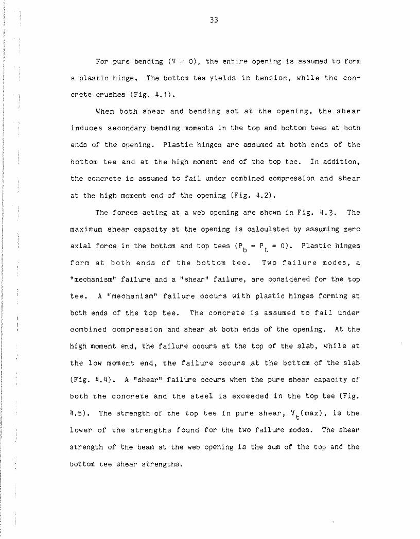
For pure bending (V = 0), the entire opening is assumed to form

a plastic hinge. The bottom tee yields in tension, while the con

crete crushes (Fig. 4.1).

When both shear and bending act at the opening, the shear

induces secondary bending moments in the top and bottom tees at both

ends of the opening. Plastic hinges are assumed at both ends of the

bottom tee and at the high moment end of the top tee. In addition,

the concrete is assumed to fail under combined compression and shear

at the high moment end of the opening (Fig. 4.2).

The forces acting at a web opening are shown in Fig, 4.3. The

maximum shear capacity at the opening is calculated by assuming zero

axial force in the bottom and top tees (Pb = Pt = 0). Plastic hinges

form at both ends of the bottom tee. Two failure modes, a

"mechanism" failure and a "shear" failure, are considered for the top

tee. A "mechanism" failure occurs with plastic hinges forming at

both ends of the top tee. The concrete is assumed to fail under

combined compression and shear at both ends of the opening. At the

high moment end, the failure occurs at the top of the slab, while at

the low moment end, the failure occurs .at the bottom of the slab

(Fig. 4. 4). A "shear" failure occurs when the pure shear capacity of

both the concrete and the steel is exceeded in the top tee (Fig.

4.5). The strength of the top tee in pure shear, Vt(max), is the

lower of the strengths found for the two failure modes. The shear

strength of the beam at the web opening is the sum of the top and the

bottom tee shear strengths.

34

Moment-shear interaction diagrams are developed by calculating

the primary moment capacity, M . , at the opening centerline as pr1mary

the shear is increased from zero to the maximum shear capacity. A

predetermined portion of the shear is assigned to the bottom and top

tees (Vb and Vt' respectively) (Fig. 4.3). Using Vb, an axial force,

Pb, and secondary bending moments, Mbl and Mbh' are calculated. Pt

and Vt are applied to the top tee (Pt = Pb and is applied in the

opposite direction). The secondary moment capacity of the high

moment end of the top tee, Mth' is then calculated. Finally,

M . is calculated using the secondary moment capacities and the pr1mary

axial force.

( 4. 1 )

in which z = the distance between the axial forces, P = Pb = Pt' a0

the opening length, and Vtotal = Vb + Vt.

The following simplifying assumptions are used:

1) The steel will yield in tension or compression.

2) Shear forces can be carried in the steel and concrete at

both ends of the opening.

3) Shear forces in the steel are carried only in the webs.

4) Shear stresses in the steel webs are uniformly distributed

over the full depth of the steel tees.

5) The normal forces in the concrete are applied over an area

defined by the 9quivalent stress block (1).

35

6) The compressive forces in the concrete are limited by the

crushing capacity of the slab, normal force equilibrium,

and the shear capacity of the shear studs between the ends

of the opening and between the opening and the supports.

The model includes provisions for web reinforcement at the

opening. In addition, the model includes provisions for solid slabs

and ribbed slabs with either transverse or longitudinal ribs.

It must be noted that, while the model is an extension of the

Clawson and Darwin model, there are significant differences. In the

Clawson and Darwin model, concrete force exists only at the high

moment end of the opening, the slab is fully composite, and reinforc-

ing steel in the slab is considered. Shear forces in the steel can

be carried in the flanges, as well as in the webs of the tees. In

addition, the Clawson and Darwin model does not include provisions

for web reinforcement and applies only to solid slab construction.

4.3 MATERIALS

Both concrete and steel are assumed to be in a state of plane

stress. The models for these materials are described below.

4.3.1 Steel

The structural steel is represented as a rigid, perfectly

plastic material. The maximum yield strength, cr , is the yield 0

stress obtained from a uniaxial tension test. No strain hardening is

considered.

36

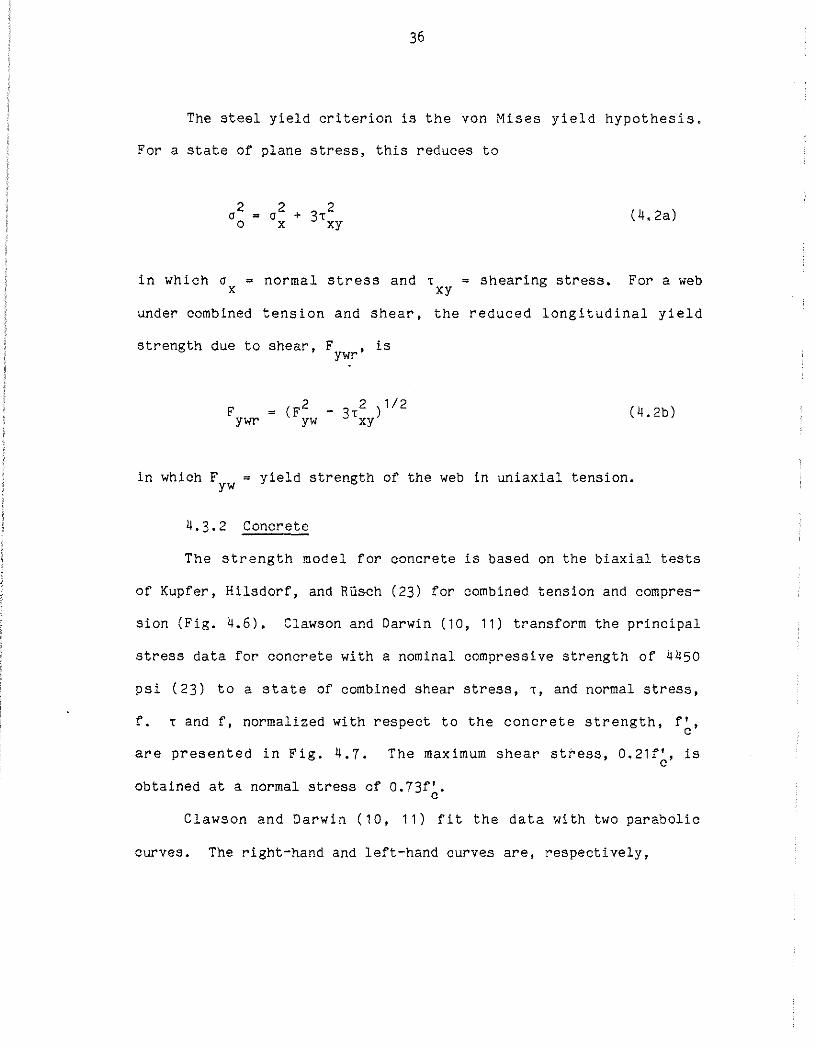
The steel yield criterion is the von Mises yield hypothesis.

For a state of plane stress, this reduces to

2 2 2 o0

= a + 3T (4.2a) x xy

in which o = normal stress and T = shearing stress. For a web x xy

under combined tension and shear, the reduced longitudinal yield

strength due to shear, F is ywr'

F = (F2 - 3T2 ) 1/2 ywr yw xy (4.2b)

in which F = yield strength of the web in uniaxial tension. yw

4.3.2 Concrete

The strength model for concrete is based on the biaxial tests

of Kupfer, Hilsdorf, and RUsch (23) for combined tension and compres-

sion (Fig. 4.6). Clawson and Darwin (10, 11) transform the principal

stress data for concrete with a nominal compressive strength of 4450

psi (23) to a state of combined shear stress, T, and normal stress,

f. T and f, normalized with respect to the concrete strength, f', c

are presented in Fig. 4.7. The maximum shear stress, 0.21f', is c

obtained at a normal stress of 0.73f~.

Clawson and Darwin ( 10, 11) fit the data with two parabolic

curves. The right-hand and left-hand curves are, respectively,

f 2 [ -2.9(f') +

c

and

T =

37

- 1.3]f' c

- 0.042]f' c

Both equations are used in the failure model.

(4.3a)

(4.3b)

The concrete is assumed to be in compression and shear at both

ends of the opening. The concrete compressive strength is limited to

0.85f, with f given by either Eq. (4.3a) or (4.3b). The normal

stress is applied over the effective width of the slab, b (defined e

in Section 4.5), while the shear stress is applied over a width equal

to 3 times the gross slab thickness, T • The nominal shear strength s

of the concrete is limited to 3.5~ (10,11).

4.4 BOTTOM TEE

The forces in the bottom tee under a positive primary moment

are shown in Fig. 4.3. These forces consist of a shear force, an

axial force, and secondary moments. Equilibrium for the bottom tee

requires that

pb = pbl = pbh

vb vbl = vbh

Mbl + Mbh = Vbao

(4.4a)

(4.4b)

(4.4c)

38

in which Pbl = the low moment end axial force, Pbh = the high moment

end axial force, Vbl = the low moment end shear force, and Vbh = the

high moment end shear force.

The web stub is assumed to extend through the flange and stiff-

ener. The shear stress in the web, Tb' is

(4.5)

in which sb = the web stub depth, and tw = the web thickness (Fig.

4.8). F and Tb are related by Eq. (4.2b) with Tb = T ywr xy

Plastic hinges are assumed to form at each end of the tee. The

equilibrium relationships (Eq. (4.4)) and the von Mises criterion

(Eq. (4.2b)) are used to express Pb as a function of Vb.

4.4. 1 Low Moment End

When a positive primary moment is applied to the web opening,

the low moment end of the bottom tee is subjected to a tensile force

and a negative secondary moment. The top of the tee is in tension,

while the bottom of the tee is in compression.

The neutral axis is assumed to be in either the web or the

flange, at a distance g, from the top of the tee (Fig. 4.9). The

neutral axis will always be below the stiffener, if the area of the

stiffener is no larger than the area of the flange.

The minimum value for g is attained when Pb = 0. As the axial

force increases with increasing primary moment, the neutral axis

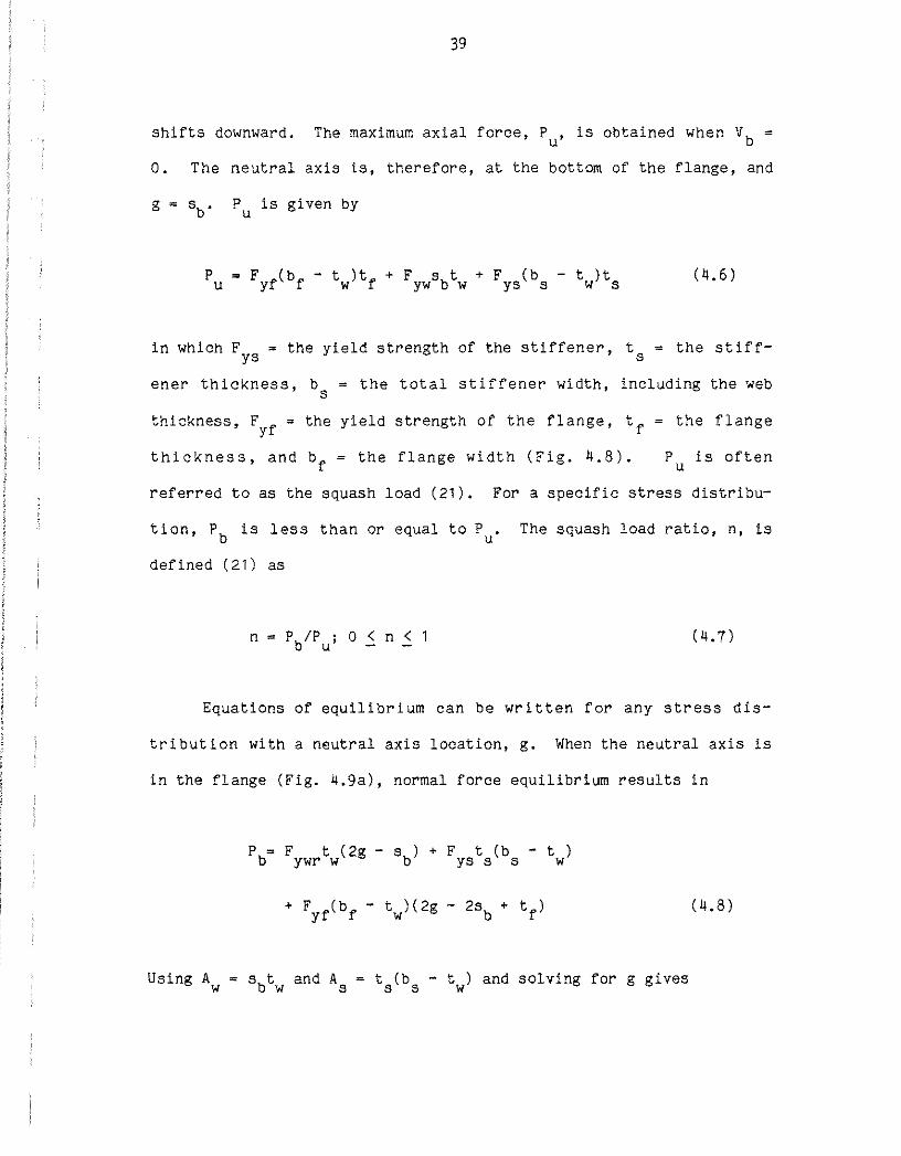
39

shifts downward. The maximum axial force, Pu' is obtained when Vb =

0. The neutral axis is, therefore, at the bottom of the flange, and

P is given by u

P = F (b - t )t + Fywsbtw + F (b - t )t u yf f w f ys s w s (4.6)

in which F = the yield strength of the stiffener, ts = the stiffys

ener thickness, b = the total stiffener width, including the web s

thickness, Fyf = the yield strength of the flange, tf = the flange

thickness, and bf = the flange width (Fig. 4.8). P is often u

referred to as the squash load (21). For a specific stress distribu-

tion, Pb is less than or equal to Pu. The squash load ratio, n, is

defined (21) as

(4.7)

Equations of equilibrium can be written for any stress dis-

tribution with a neutral axis location, g. When the neutral axis is

in the flange (Fig. ~.9a), normal force equilibrium results in

Pb= F t (2g - sb) + F t (b - t ) ywr w ys s s w

= t (b - t ) and solving for g gives s s w

(4.8)

40

Moment equilibrium requires that

2 s = F t c.-.E

ywr w 2 2

- g ) - F A y ys s s

(4.9)

(4.10)

Combining Eq. (4.6), (4.7), (4.9), and (4.10) gives Mbl in terms of

n.

(4.11a)

(A F + A F + A F ) f yf w yw s ys in which 2(F t + F f(bf ~ t )) ywr w y w

(4.11b)

F A - F A + F f(bf - t )(2sb - tf) ywr w ys s y w (4.11c)

cf3

= - F t - F (b - t ) ywr w yf f w (4.11d)

and

(4.11e)

41

When the neutral axis is in the web (Fig. 4.9b), normal force

equilibrium gives

P = Fywrtw(2g - s ) + F t (b - t ) b b ys s s w

Using Af

g = P ~ F A + F A + F A

b ys s ywr w yf f 2F t ywr w


2 sb

= F t (-ywr w 2

(4.12)

(4.13)

(4.14)

Combining Eq. (4.6), (4.7), (4.13), and (4.14) gives Mbl in terms of

n.

Mbl 2 2

+ 2Cw,Cw2cw3n + 2

+ cw4 (4.15a) = Cw,Cw3n cw2cw3

Al Y.f + A F + A F in which cw1 =

W 'f.W s ys (4.15b) 2(Fywrtw)

F A - F A + FytAf cw2

'f.Wr w ys s (4.15c) 2(Fywrtw)

42

C = - F t w3 ywr w (4.15d)

and s

FywrAw 2b- FysAsys + FyfAf(sbtf/ 2) (4.15e)

Eq. (4.11a) anr! (4.15a) are quadratic equations in n. For any

value of Mbl' therefore, the corresponding axial force, Pb = nPu, can

be found.

The neutral axis crosses over from the flange to the web when

when g = sbtf. Substituting for gin Eq (4.12) gives

(4.16)

Substituting for Pb in Eq. (4.7) and consolidating terms gives

F t (s -ywr w b + F A + F A ) ywr w ys s

(4.17)

f in which nxl = the flange to web crossover ratio at the low moment

end of the bottom tee.

4.4.2 High Moment End

When the opening is subjected to a positive primary moment, the

high moment end of the bottom tee is subjected to a tensile force and

43

positive secondary moment. Therefore, the top of the tee will be in

compression, and the bottom of the tee will be in tension.

The neutral axis is located a distance g from the top of the

tee. Unlike the low moment end, the neutral axis can be located

anywhere within the stub depth (Fig. 4.10).

The maximum value for g is attained when Pb = 0. As the ten

sion force is increased under increasing primary moment, the neutral

axis shifts upward. Based on normal force and moment equilibrium,

equations giving Mbh in terms of n are developed.

When the neutral axis is in the web above the stiffener (Fig.

4.10a), normal force equilibrium requires that

P = F t (sb - 2g) + F (b - t )t b ywr w ys s w s

(4.18)


M Ca2

1ca3

n2 2C c c c2 c c bh = - a1 a2 a3n + a2 a3 + a4 (4.19a)

in which (AfFyf + A F + A F )

C = _..:_..;._..:_=-;;"w~y-:wc,_..::s~y..::s:..... a1 2(F t) ywr

(4.19b)

(4.19c)

44

C = - F t a3 ywr w (4.19d)

and (4.19e)

When the neutral axis is in the stiffener (Fig. 4.10b), normal

force equilibrium requires that

Pb = F t (sb- 2g) + 2F (b - t )(y -g) ywr w ys s w s

(4.20)


Mbh c2 c 2 - 2Cs1cs2cs3n +

2 + cs4 (4.21a) = cs2cs3 s1 s3n

(Al yf + A F + A F ) in which cs1 =

w y_w s ys (4.21b) 2(F t + F (b - t ) ) ywr w ys s w

A F + A F + 2F ( b - t )y cs2 =

f yf w y_wr y_s s w s (4.21c) 2(F t + F (b - t )) ywr w ys s w

C = - F t - F (b - t ) s3 ywr w ys s w (4.21d)

and cs4 = FyfAf(sbtf/2) + F A sb

ywr w 2

F (b - t ) t /2) 2

+ (y - t /2) 2) + y_s s w ( (y + (4.21e) 2 s s s s

45

The neutral axis crosses over from the web above the stiffener to the

stiffener when g ~ ys- ts/2. Substituting for gin Eq. (4.18) gives

(4.22)

Substituting for Pb in Eq. (4.7) and consolidating terms gives

(4.23)

s in which nxh ~ the squash load ratio at crossover from the web above

the stiffener to the stiffener at the high moment end of the tee.

If the neutral axis is in the web below the stiffener (Fig.

4.10c), the moment-axial force equation for the high moment end is

M Cw2

1cw3n2 2C c c c2 c c bh = - w1 w2 w3n + w2 w3 + w4 (4.24)

in which the coefficients are given by Eq. (4.15b) - (4.15e). The

neutral axis crossover from the stiffener to the web below the stiff-

ener occurs when g ~ y + t /2. Therefore, the squash load ratio at s s

w crossover, nxh' is

w F t (s - 2y - t ) + F A - F A ywr w b s s yf f ys s n = xh (F A + F A + F A ) yf f yw w ys s

(4.25)

46

If the neutral axis is in the flange (Fig. 4.10d), the moment-axial

force equation for the high moment end is

(4.26)

in which the coefficients are given by Eq. (4.11b)- (4.11e). The

web-flange crossover occurs when g = sb - tf. Therefore, the squash

load ratio at crossover, n~h' is

F t (2tf -ywr w + F A + F A ) ~w ~s

(4.27)

Eq. (4.19a), (4.21a), (4.24) and (4.26) are quadratic equations

inn. For any value of Mbh' the corresponding axial force, Pb =

nP can be found. u

4.4.3 Total Capacity

Moment-axial force equations are developed by substituting Eq.

(4.11a) or (4.15a) for Mbl and Eq. (4.19a), (4.21a), (4.24), or

(4.26) for Mbh in Eq. (4.4c). The neutral axis may be located within

one of two regions at the low moment end (Fig. 4.9a and 4.9b), while

the neutral axis may be located within one of four regions at the

high moment end (Fig. 4.10a-4.10d). Thus, a total of eight possible

moment equilibrium relationships exist. The correct neutral axis

locations at the low and high moment ends must be found by trial.

47

The procedure for establishing the neutral axis locations is

described in Appendix C.

Once the neutral axis locations are established, a moment-axial

force equation (selected from Eq. (C,1)~(C,7)) is obtained. n is

determined by solving the equation, which is a quadratic in terms of

n. Mbl is then calculated using Eq. (4,11a) or (4,15a) and Mbh is

calculated using Eq. (4,19a), (4.21a), (4.24), or (4.26). Finally,

Pb is calculated using Eq. (4.7).

4.5 TOP TEE

The forces and moments acting in the top tee under a positive

moment are shown in Fig, 4.3. As with the bottom tee, these include

a shear force, an axial force, and secondary moments.

Equilibrium for the top tee requires that

(4.28a)

(4.28b)

(4.28c)

in which Ptl = the low moment end axial force, Pth = the high moment

end axial force, Vtl = the low moment end shear force, and Vth = the

high moment end shear force.

Shear can be carried by both the steel tee and the slab.

v = v + v t c s (4.29)

48

in which V c the portion of the top tee shear carried by the con-

crete and Vs = the portion of the top tee shear carried by the web of

the steel tee.

The shear stress in the steel web, 's• is

T = V /(stt ) (4.30) s s w

in which st =the web stub depth (Fig. 4.11). F for the top tee ywr

web and T are related by Eq. (4.2b) with T = T s s xy

The concrete can carry shear in the compression zone at both

ends of the opening. The concrete is assumed to be in compression at

the bottom of the slab at the low moment end and at the top of the

slab at the high moment end. As with Clawson and Darwin's model, the

shear is carried in a width equal to 3 times the gross slab thickness

(10, 11). The shear stress in the concrete is

v c 'c = 3T c

s (4.31)

in which Ts = the total (gross) slab thickness, and c = the distance

from the neutral axis to the extreme compressive fiber in the

concrete. The compressive stress in the concrete is carried over

width b (2). e

b < Span/4 e-

< Beam spacing

<16Ts+bf

< Slab width

49

(4.32)

c is selected such that for given shear and normal forces, the

concrete stresses comply with Eq. (4.3a) or (4.3b). It should be

noted that, in general, c will not be the same at both ends of the

opening.

In the top tee, all of the shear is assumed to be applied to

the steel web, if the applied shear is less than or equal to the

plastic shear capacity of the web, Vpt

shear in excess of Vpt" For the top tee,

stt F 1/3 w y

The concrete carries any

(4.33a)

The upper bound of the shear that can be applied to the top tee

is the "pure shear" capacity for the top tee, V t ( sh).

3.5/fl A c cv 1000

+ V , kips pt (4.33b)

in which A = 3T t and t = the effective slab thickness. te is cv s e e

dependent on the type of slab. For ribbed slabs with the ribs per-

pendicular to the beam,

50

te = ts = the minimum slab thickness

For ribbed slabs with the ribs parallel to the beam,

T +t s s 2

= the average of the maximum and

minimum slab thicknesses

For solid slabs,

t = T the slab thickness e s

(4.34a)

(4.34b)

(4.34c)

Normal forces exist in the steel tee and in the slab.

Equilibrium requires that

P cl + p sl (4. 35a)

= P ch + P sh (4.35b)

in which P01 = the low moment end concrete force, Pch =the high

moment end concrete force, Psl = the low moment end steel force, and

Psh =the high moment end steel force. Pch is given by

P h < NRQ c - n

< p c

51

(4.36a)

(4.36b)

(4.36c)

in which N = the number of studs between the high moment end of the

opening and the support, R = the reduction factor for studs in ribbed

slabs, Q = the nominal strength of one stud shear connector embedded n

in a solid slab (3, 29), Pc =the crushing capacity of the slab

(reduced for V ), and P = the maximum capacity of the top tee c smax

steel (reduced for Vs). P01

is given by

P = P - N RQ > 0 cl ch o n - (4.37)

in which N = the number of shear connectors above the opening. 0

For slabs with transverse ribs, R is (2, 3, 20)

R w H

.85(.2:)(hs - 1.0) < 1.0 IN hr r

r

(4.38)

in which hr = the nominal rib height in inches, Hs = the length of

the stud connector after welding in inches, N = the number of stud r

connectors in one rib, and w = the average width of the concrete r

rib.

For slabs with ribs parallel to the steel beam, the reduction

factor is (2, 3, 20)

54

compression. The top of the steel tee is in tension, while the

bottom of the tee is in compression.

From Eq. (4.35a), the force in the steel at the low moment end,

Psl' is given by

P sl = P t - P cl (4.46)

The neutral axis in the steel tee is located at a distance g

from the bottom of the tee (Fig. 4.13). The neutral axis can be

located anywhere within the steel tee at the low moment end.

When the neutral axis is in the web below the stiffener (Fig.

4.13a), normal force equilibrium requires that

-FyfAf - F t (s - 2g) - F A ywr w t ys s (4.47)

The neutral axis crosses over from the web below the stiffener to the

ts stiffener when g = ys - 2· The force in the steel at crossover,

s P xl' is

(4.48)

s If P sl < P xl' the neutral axis is in the web below the stiff-

ener and

57


- F A y - P y ys s s cl cl (4.58)

f If Psl > Pxl' the neutral axis is in the flange (Fig. 4.13d)

and

g P81 + F (b - t )(2s - t ) + F A - F A yf f w t f ywr w ys s

2(F f(bf - t ) + F t ) y w ywr w (4.59)


+ F t

ywr w ( 2 2 st 2g2) - F A y - P y ys s s cl cl (4.60)

4.4.1.2 High moment end

When the opening is subjected to a positive primary moment, the

high moment end of the top tee is subjected to a compressive force

and a positive secondary moment. At the maximum "mechanism" shear

load, the top tee is subjected only to a positive secondary moment.

In either case, the top of the concrete slab is in compression.

58

Also, the top of the steel tee is in compression while the bottom of

the tee is in tension.

From Eq. (4.35b), the force in the steel at the high moment

end, P sh' is

P sh = P t - P ch (4.61)

The neutral axis is located a distance g from the bottom of the

tee (Fig. 4.14). Unlike the low moment end, the neutral axis is

assumed to be above the stiffener in one of only two regions. This

is always true, if the area of the stiffener is no larger than the

area of the flange.

When the neutral axis is in the web (Fig. 4.14a), normal force

equilibrium requires that

The web-flange crossover occurs when g = st - tf" The force in the

f steel at crossover, Pxh' is

(4.63)

f If Psh > Pxh' the neutral axis is in the web at the high moment end

(Fig. 4.14a). Therefore,

59

g = 2F t

If F = 0, then ywr

g = s - t t f

ywr w


F t ywr w 2

- F A ys s (4.64a)

(4.64b)

(4.65)

f If P sh < P xh' the neutral axis is in the flange at the high moment

end (Fig. 4.14b). The neutral axis location is given by

g = -Psh + F f(bf ~ t )(2st - tf) + F A - F A y w ywr w ys s

2(F f(bf - t ) + F t ) y w ywr w

and the high moment end secondary moment is

+ F t ywr w

2

(4.66)

(4.67)

60

4.6 DETAILS OF INTERACTION PROCEDURE

The initial step in developing an interaction diagram is to

find the shear capacities of the bottom and top tees.

The bottom tee shear strength, Vb(max), is calculated by vary

ing the shear force in the tee (using bisection) until zero normal

force exists in the tee.

The top tee shear strength, Vtm' is the minimum of the

"mechanism" strength, Vt(max), and the "pure shear" strength, Vt(sh).

The "mechanism" strength is calculated by varying the shear force in

the tee (using bisection) until moment equilibrium, Eq. (4.28c) is

satisfied for the tee. Shear is applied to the slab only if the

total shear required to satisfy moment equilibrium is greater than

Vpt If the concrete forces are too high for moment equilibrium to

be satisfied, the high moment end concrete force is incrementally

reduced until Eq. (4.28c) is satisfied (The difference between P ch

and P01 is maintained using Eq. (4.37)). The "shear" strength is

found using Eq. (4.33b).

The total shear strength, Vm, is the sum of Vb(max) and Vtm•

The interaction diagram is developed by assigning to the opening

incrementally larger values of shear from 0 to V • As the shear is m

increased from 0 to 90 percent of Vtm' all of the shear is assigned

to the top tee (Fig. 4.15). The top tee shear, Vt, is then varied

linearly from 90 to 100 percent of Vtm [Vt = qVtm (0.9 < q ~ 1.0)] as

the bottom tee shear, vb, is increased quadratically from 0 to 10

percent of Vb(max).

61

0.10Vb(max)(1 - /1 - q') (4.68a)

in which

q' = 100(q- 0.9) 2 (4.68b)

Additional shear is assigned to the bottom tee only (Fig. 4.15).

This procedure was selected to provide a good match with test

results, as well as a reasonable shape for the interaction diagram.

Since the overall method is an equilibrium procedure, the interaction

diagrams represent lower bound solutions.

The axial force in the top and bottom tees is governed by the

bottom tee. At an assigned value of bottom tee shear, an axial force

and secondary bending moments are calculated. An axial force of

equal magnitude but opposite direction is applied to the top tee.

The top tee shear force is applied, and the high moment end secondary

moment is calculated.

The low moment end secondary moment is not calculated at top

tee shears lower than Vtm• At these shears, the low moment end will

not be completely plastic at the maximum high-moment-end secondary

moment.

The primary moment at the opening centerline (Eq. (4.1) and

Fig. 4.3) is

using z = h . 0

(4.69)

62

The shear capacities of the top and bottom tees are calculated

at zero axial force. The point of contraflexure in the top tee,

however, will not be at the opening centerline. Therefore, M . pr1mary

will be greater than zero. In order to complete the interaction

diagram, a value of total shear must be calculated for zero primary

moment. This is done using the procedure used by Clawson and Darwin

(10, 11). The top tee shear is held constant at Vtm' while the

bottom tee shear is decreased slightly. A compressive axial force is

then applied to the bottom tee, and a tensile axial force is applied

to the top tee such that

(4.70)

4.7 COMPARISON WITH TEST RESULTS

The model is used to predict the strength of the 15 tests in

the current study along with the 22 prior tests. Ratios of test to

calculated strength are tabulated in Table 4.1. Interaction curves

for the model are compared with the test data from the current tests

in Figs. 4.16 to 4.30.

The interaction curves are calculated using the material

strengths, beam geometries, and shear stud quantities summarized in

Chapter 2 and Appendix 8. The experimental web, flange, and stiff-

ener yield strengths are used in the calculations.

For the beams with solid slabs tested by Clawson and Darwin (9,

11), the calculations indicate that the stud capacities are limited

63

by the tensile strength of the shear connectors ( Eq. ( 4. 41)). For

these calculations, a strength of 60 ksi (a typical industry minimum)

is used, since the actual strengths are not known. It is important

to note that no stud failures were observed in any of the tests.

In addition to the individual comparisons, Table 4.1 includes

the means and standard deviations of the test/theory ratios for each

test series, for each slab type (ribbed or solid), and for all of the

tests. The ratios for Tests 4A and 4B for the current series are not

included in these calculations. These tests had no shear connectors

above the opening, but did have puddle welds in each rib. It was

found that the puddle welds in the ribs above the openings trans

ferred significant shear between the top tee steel and the slab.

Since the tabulated ratios for Tests 4A and 4B are based on zero

shear transfer above the openings, they do not provide a fair measure

of model accuracy.

The interaction diagrams emphasize a point that has been made

before (9, 10, 14); that is, the interaction between moment and shear

capacity at a web opening is rather weak. The moment capacity at a

web ope~ng is largely unaffected by shear until the shear reaches

the maximum shear capacity.

The strength model provides exceptionally good agreement with

the experimental results. For beams with ribbed slabs, the mean and

standard deviation are 1.023 and 0.070, respectively. For beams with

solid slabs, the mean and standard deviation are 1.074 and 0.060,

64

respectively. The overall mean and standard deviation fer the model

are 1.042 and 0.071.

The lowest individual test/theory ratio is 0.904 (Test RO), In

addition to Test RO, Test 1 has a particularly low test/theory ratio

(0.919). For both tests, the deviation may be the result of the load

history of the tests. Both tests were loaded above initial yield,

unloaded, and then reloaded to failure. In the initial cycle, sig

nificant twisting of the beams was noted. In the model, however,

cyclic effects and out of plane bending are not considered.

Tests 8A, BB, and 9A also have relatively low test/theory

ratios. These tests had relatively stiff slabs and had a low number

of studs over the opening. The stiff slabs tended to pull away from

the steel tees, resulting in bridging of the slab. As a result of

the bridging, the failure point in the concrete slab was close to the

to the load point, while the model assumes failure at the high moment

end of the opening, Also, the studs over the opening may have failed

primarily in tension, rather than in shear. The model does not

include provisions for interaction between tension and shear in the

studs above the opening.

In general, tests with solid slabs have high test/theory

ratios. In the tests conducted by Clawson and Darwin (9, 11), no

stud failures were noted. The stud forces used in the model,

however, are limited by the assumed tensile capacities of the studs.

It is likely that the studs had higher tensile capacities than the

assumed capacities.

65

Tests 3, R3, R4, and C3 had high M/V ratios. Three of these

tests, R3, R4, and C3 failed at relatively high test/theory ratios.

This is probably the result of the representation of the steel in the

tees. In tests with high M/V ratios, the steel sections were sub

jected to high tensile strains (well over 2 percent). The steel was,

therefore, in the strain hardening range. The model, however, has no

provisions for strain hardening. The effect of strain hardening in

high shear tests will be lower, because of the high strain gradients

in the steel tees. Test 3 had a relatively low test/theory ratio

when compared with the other tests with high M/V ratios. This may be

the result of cyclic loading during the test. Test 3 was loaded

above initial yield, unloaded, and reloaded to failure (The initial

cycle was terminated to allow adjustment of the load system).

The following chapter presents practical design techniques that

were developed based on lessons learned with the model. The model

results are compared with the results obtained with the practical

design techniques, as well as with the Redwood and Poumbouras (33)

analysis procedure.

5.1 GENERAL

66

CHAPTER 5

STRENGTH DESIGN PROCEDURES

While the strength model presented in Chapter 4 provides good

agreement with test results, it is not well suited for design. The

"mechanism" shear capacity must be found by iteration, and the inter

act ion diagram is calculated "point by point". Therefore, the model

requires the use of a computer. A useful design procedure should

require no more than a programmable calculator.

A number of design procedures for composite beams with unrein

forced openings have been proposed (11, 33, 34). In all cases, the

maximum moment capacity is found using the standard strength proce

dures developed by Slutter and Driscoll (35). The procedures differ

in the methods used to find the maximum shear capacity at the opening

and the methods used to construct moment-shear interaction curves.

The methods used to establish the maximum shear capacity are

based on local moment equilibrium (11, 33, 34). A four hinge

mechanism is assumed at the opening, and moment equilibrium is en

forced for the bottom and top tees. The methods differ in the

simplifying assumptions used to reduce the complexity of the calcula

tions and in the forces assumed in the concrete slab. The methods

also differ in the limiting shear at the opening corresponding to a

"pure" shear failure.

67

Clawson and Darwin (11) have proposed a design procedure which

enforces local equilibrium but which requires iteration. In the top

tee, the concrete is assumed to crush at the high moment end and to

be fully cracked at the low moment end. The shear capacity is

limited by the pure shear capacities of the webs and the concrete.

The moment-shear interaction diagram is obtained by connecting the

maximum shear and moment capacities with an ellipse. Clawson and

Darwin (11) show that the design procedure provides reasonable agree

ment with the results of tests of composite beams with solid slabs.

Redwood and Wong (34) show that the procedure also gives reasonable

agreement with the results of tests on composite beams with ribbed

slabs. Because the procedure requires iteration, however, any prac

tical applica~ion to design requires the use of a computer.

Redwood and Wong (34) have proposed a procedure which does not

enforce local equilibrium. The flange thicknesses are assumed to be

small relative to the depths of the tee section webs above and below

the opening. Equilibrium of normal forces in the tees is not

enforced. The concrete force at the high moment end is limited by

the shear capacity of the stud connectors above the opening. Zero

force is assumed in the concrete at the low moment end. A closed

form solution is obtained. The shear capacity is limited by the pure

shear capacity of the top tee and bottom tee webs.

The maximum shear and the maximum moment that can be sustained

at the maximum shear are calculated, generating a vertical line on

the right side of the interaction curve. The curve is closed with an

68

ellipse between the maximum moment at zero shear (found considering

partial composite action) and the maximum moment at the maximum

shear. Because the interaction curve is not continuous, calculation

of the capacity for a given H/V ratio is somewhat cumbersome, The

procedure is very conservative for openings with low H/V ratios in

beams with either solid or ribbed slabs. The Redwood and Wong proce

dure has been used by u.s. Steel (44) as the basis of a design aid.

Redwood and Poumbouras (33) have proposed a modification of

Redwood and Wong's procedure which provides a good match with test

results on composite beams with ribbed slabs. The method includes

provision for a compressive force in the concrete at the low moment

end of the opening, which is set equal to the total shear connector

capacity between the opening and the support.

The interaction curve is similar to the curve used by Redwood

and Wong. The maximum shear and the maximum moment that can be

sustained at the maximum shear are calculated, generating a vertical

line on the right side of the interaction curve. The curve is closed

with an ellipse between the maximum moment at zero shear (assuming

full composite action) and the maximum moment at the maximum shear.

The maximum moment at zero shear (considering partial composite

action) is calculated, generating a horizontal line between zero

shear and the interaction curve. The calculation of the capacity for

a given M/V ratio is, therefore, even more cumbersome than for the

Redwood and Wong procedure.

69

The Redwood and Poumbouras procedure is the most accurate of

the three existing procedures for beams with ribbed slabs. However,

it is very conservative at high shears for beams with solid slabs.

The existing design procedures have limitations. While the

Clawson and Darwin procedure can produce good agreement with test

results for beams with solid or ribbed slabs, it requires the use of

a computer. The procedures proposed by Redwood and others are easier

to apply, but they are very conservative when applied to solid slab

construction. There is, therefore, a need for comprehensive design

procedures which give consistent agreement with test results and are

easily applied.

5.2 OVERVIEW OF DESIGN PROCEDURES

Three design procedures are presented which allow the rapid

construction of moment-shear interaction diagrams for composite

beams. The proposed methods require the calculation of the maximum

moment capacity, M , and the maximum shear capacity, V , at a web m m

opening in a composite beam. The calculation of these points and the

application of an interaction equation are discussed in the following

sections.

The procedures are based on the following assumptions:

1) The steel will yield in tension or compression.

2) Shear forces can be carried in the steel and concrete at

both ends of the opening.

3) Shear forces in the steel are carried only in the webs.

70

4) Shear stresses are uniformly distributed over the stub

depth.

5) The normal forces in the concrete are applied over an area

defined by the equivalent stress block (1).

Fig. 5.1 illustrates openings in composite beams with a solid

slab, a ribbed slab with the ribs transverse to the beam, and a

ribbed slab with the ribs parallel to the beam. The openings are of

length a and depth h and may have an eccentricity e (positive 0 0

upward) with respect to the centerline of the steel section. The

slab thicknesses, Ts and ts, effective slab width, be' and steel

section dimensions, d, bf, tf, tw' st' and sb, are as shown.

5.3 INTERACTION CURVE

Once M and V have been obtained, intermediate values of shear m m

and moment are obtained using an interaction curve of the form

M 3 lM n) +

m ( 5. 1 )

in which Vn = the nominal shear capacity and Mn = the nominal moment

capacity at a web opening in a composite beam (Fig. 5.2). The

nominal capacities can be determined for a given ratio of moment to

shear, M/V, as follows. From Eq. (5.1),

M 3 V 3 (...!!) (..1!.!) + 1 M V (5.2)

m n

71

Letting M /V = M/V and solving for v yields n n n

(!:!)3 -1/3

v = v v + 1 (5.3) n m M 3

(2!) v m

and

M v (!:!) ( 5. 4) n n v

M 3 -1/3 (2!)

M v + 1 (5.5) m m

(!:!)3 v

The complete interaction curve is described by a single

function. This is conceptually sound since the interaction between

moment and shear should be continuous. It also allows a single

equation to be used to calculate the nominal shear capacity at a

given M/V ratio. Thus, the application of the procedure is simple.

As will be shown, Eq. (5.1) provides good agreement with test

results.

5.4 MAXIMUM MOMENT CAPACITY

The maximum moment capacity, M , of a composite beam at a web m

opening is obtained using the strength procedures developed by

Slutter and Driscoll (35). Fig. 5.3 illustrates stress diagrams for

sections in pure bending. The steel section is assumed to be fully

plastic in both tension and compression, while the compressive force

72

in the concrete, Pch' is limited by 1) the crushing capacity of the

slab, P , 2) the shear capacity of the stud connectors between the c

high moment end of the opening and the support, Pstuds' and 3) the

yield capacity of the net steel section, T'.

p < p Ch - C

< p - studs

< T'

(5.6a)

(5.6b)

(5.6c)

The concrete stress is assumed to be at 0.85f' over the depth c

of the equivalent stress block.

The crushing capacity of the slab is

P = o.85f'b t c c e e (5.7)

in which f' = the compressive strength of the concrete in ksi, b = c e

the effective slab width (2), and t = the effective slab thickness. e

te is dependent on the type of slab. For ribbed slabs with the ribs

perpendicular to the beam,

t = t = the minimum slab thickness e s (5.8a)

For ribbed slabs with the ribs parallel to the beam,

t = e

T +t s s

2

73

= the average of the maximum and

For solid slabs,

t e

minimum slab thicknesses.

T = the slab thickness. s

The shear capacity of the stud connectors is

P = NRQ studs n

(5.8b)

(5.8c)

(5.9)

in which N = the number of studs between the high moment end of the

opening and the support, R = the reduction factor for studs in ribbed

slabs, and Qn = the nominal strength of one stud shear connector

embedded in a solid slab (3, 29).

For slabs with transverse ribs, R is (2, 3, 20)

R = - 1.0) < 1.0 (5.10a)

in which h = the nominal rib height in inches, H r s

the length of

the stud connector after welding in inches, N = the number of stud r

74

connectors in one rib, and w r

the average width of the concrete

rib.

For slabs with ribs parallel to the steel beam, the reduction

factor is (2, 3, 20)

R = < 1.0 (5.10b)

For solid slab construction, R = 1.0.

Qn is given by

Q = 0. 5A If' E n sc c c (5.11a)

in which A = the cross-sectional area of a stud shear connector, sc

f' = the compressive strength of the concrete in ksi, E = the c c

modulus of elasticity of the concrete in ksi and is given by

f' in psi c

The product RQ is limited such that n

RQ < A F n- sc u

(5.11b)

(5.12)

in which F = the minimum tensile strength of a stud in ksi (2, 3, u

29).

75

Under pure bending, the shear is zero; therefore, the web yield

strength is not reduced. The yield capacity of the net steel section

is

T' ~ F (2(b - t )t + s t + s t ) y f w f t w b w (5.13)

in which Fy = the yield strength of the section, bf ~ the flange

width, tw ~ the web thickness, tf = the flange thickness, st = the

top tee stub depth, and sb ~ the bottom tee stub depth (Fig. 5. 1).

For solid slabs or for ribbed slabs with transverse ribs, the

depth of the stress block is

Pch a = ~=-=;:,:,--0.85f' b c e

Pch acts at a distance dh from the top of the flange.

(5.14)

(5.15)

-For ribbed slabs with longitudinal ribs, Eq. (5.15) will hold if a<

ts. If a> ts' dh must be calculated by considering the concrete

below the top of the steel deck.

The expression used to calculate M depends on which of the m

inequalities in Eq. (5.6) governs. If P ch = T' (Eq. (5.6c) and Fig.

5.3(a)), the maximum moment capacity is

76

M = Pchdh + FY(bf- tw)tfd m

2 2 st - s b

+ s d) + F t ( 2 y w b (5.16)

If P ch < T' (Eq. (5.6a) and (5.6b)), the neutral axis will be

in the steel tee. The compressive force in the steel is

T' - p ch c' = -~---=;:.:

2 (5.17)

The neutral axis location in the top tee, x, is measured from the top

of the steel section. If c• ~ Fybftf (Fig. 5.3(b)), x < tf and is

given by

(5.18)

and

(5.19)

(5.20)

and

s 2 + F t ( t

y w

5.5 MAXIMUM SHEAR CAPACITY

77

(5.21)

All current strength procedures for composite beams with web

openings use a "mechanism" failure mode as one of the limits for the

shear capacity ( 11, 33, 34). The "mechanism" mode is based on the

formation of plastic hinges at both ends of the top and the bottom

tees. Shear and normal stresses in the steel are limited by the von

Mises yield criterion. Normal stresses in the concrete are limited

to 0.85f~.

A closed-form solution for the maximum shear capacity at a web

opening requires the use of one or more simplifying assumptions.

Some of these simplifications are:

1) Using simplified versions of more detailed material models,

2) Limiting the neutral axes locations in the steel tees to a

specified range, and

3) Ignoring local equilibrium within the tees.

Three procedures for estimating the maximum shear capacity are

presented in the following sections. Each procedure uses one or more

simplifications. The three procedures share a common basis.

Vm is found by assuming that

( 5. 22)

78

in which Pt = the top tee force and Pb = the bottom tee force at the

opening (Fig. 5.4). This approximates zero moment at the centerline

of the opening. The moment is not exactly zero because the secondary

bending moments in the top tee, Mth and Mtl' are not equal.

Therefore, while the primary moment (= Pz) is zero, the total moment

at the centerline of the opening has a small but finite value.

The normal forces in the concrete at the ends of the opening,

Pch and P01 , are limited by the shear stud capacities between the

ends and the nearest support. The high moment end force, P ch' is

located near the top of the slab, and the low moment end concrete

force, P cl' is located near the bottom of the slab (Fig. 5.5). This

assumption is also used by Redwood and Poumbouras (33). It agrees

with test observations and, for given values of P ch and P cl' maxi

mizes the calculated shear at a web opening. Normal stresses in the

concrete are fixed at o.85f', and are represented using the equivc

alent stress block. The effect of shear stress on the normal

stresses in the concrete is ignored.

The maximum force in the concrete at the high moment end of the

opening is

(5.23a)

(5.23b)

in which P and P t d are given by Eq. (5.7) and Eq. (5.9), c s u s

respectively.

79

The force in the concrete at the low moment end of the opening

is

(5.24)

in which N0

= the number of shear studs over the opening. R and Qn

are given in Eq. (5.9)-(5.12).

P ch acts at a distance dh from the top of the flange. dh is

given by Eq. (5.14). P01 acts at a distance d1 from the top of the

flange. For slabs with transverse ribs, d1

is given by

0.5P01 0.85f' b c e

For solid slabs, d1

is given by

0.5Pcl

o.85f~ be

(5.25a)

(5.25b)

For slabs with longitudinal ribs, d1

is the distance to the centroid

of the concrete force in the trapezoidal ribs within be (Fig. 5.1).

In the top tee, all of the shear is assumed to be applied to

the web if the applied shear is less than or equal to the plastic

shear capacity of the web, Vpt" The concrete carries any shear in

excess of Vpt" For the top tee,

stt F 1/3 w y (5.26)

80

The upper bound of the shear that can be applied to the top tee

is the "pure shear" capacity for the top tee, Vt(sh).

3. siF A c cv V t ( sh) = __ 1_0;;.00__::;.:. + vpt , kips

in which A = 3T t and te is given by Eq. (5.8). cv s e

(5.27)

In the bottom tee all of the shear is assumed to be carried by

the web.

5.5. 1 Maximum Shear Capacity- Method I

Fig. 5.5 illustrates the stress distributions at the opening

for a mechanism failure. The steel section is assumed to be fully

plastic in both tension and compression. In both the top and bottom

steel tees, the neutral axis is assumed to be in the flange. The

flange yield strength, Fyf' is not reduced for shear, since the shear

is assumed co be carried by the web. The web yield strength, F ywr'

is reduced for shear. F ywr is obtained using a linear approximation

of the von Mises criterion (Fig. 5. 6). Normal force equilibrium is

enforced in the top tee steel, but equilibrium is not necessarily

enforced at the concrete-steel interface.

The von Mises criterion (Eq. (4.2)) is

(5.28a)

81

A dimensionless form of the von Mises surface, f(x), x =

given by

f(x) T

= (_!l) = cr

0

_1 ( 1 -

13

cr Ia , is X 0

(5.28b)

f(x) is quadratic. Several methods can be used to approximate

f(x) with a straight line, including least squares, near minimax, and

minimax approximations (12). The minimax approximation (also known

as the best uniform approximation) provides a line, p(x), that is the

same distance from f(x) at three locations for 0 < x < 1. The dis-

tance has alternate changes of sign in this interval (Fig. 5.6).

p(x) minimizes the norm, J Jf - pJ J~, given by

II f - PI I~ max I I 0 < x < 1 f(x) - p(x)

In this case, p(x) is given by

p(x) = T

(_!l) = cr

0

.69692

for which the norm on the interval 0 < x < 1 is

!If- PI I .. = o.11957

(5.29)

(5.30)

(5.31)

82

f(x) and p(x) are illustrated in Fig. 5.6. Eq. (5.30) can also be

expressed as

(5.32a)

in which A= 1.207.

Therefore, the reduced yield strength for the web due to shear, Fywr'

is

F = AF - /3T ywr yw xy (5.32b)

in which F = the yield strength of the web in uniaxial tension. yw

Eq. (5.28) limits Txy such that

T < a0!/3 = 0.58a

0 (5.33) xy -

compared to a maximum of 0.70a0

in Eq. (5.32). Eq. (5.33) is used as

an upper bound on the application of Eq. (5.32), at the limit F = ywr

0 (Fig. 5.6).

Since Vm is found by assuming that Pt = 0, normal force equi

librium between the steel tee and the slab requires that, in addition

to the restrictions placed on Pch by Eq. (5.23),

p < p ch- smax (5.34a)

83

in which P = the tensile capacity of the top tee. smax

p smax (5.34b)

It should be noted that the effect of shear stress on the normal

stress in the web is not included in P • smax

5.5.1.1 Bottom Tee

The shear capacity of the bottom tee is obtained by finding the

plastic moment and shear force that satisfy moment equilibrium for

the bottom tee (Eq. (4.4c)).

in which Vb = the bottom tee shear, Mbl = the secondary moment at

the low moment end of the opening, and Mbh = the secondary moment at

the high moment end of the opening. When Pb = 0,

(5.36)

and

(5.37)

in which Mb = the secondary moment at each end of the opening.

84

The neutral axis location is assumed to be in the flange, at a

distance, g, from the bottom of the flange (Fig. 5.5). Normal force

equilibrium (Pb = 0) results in

(5.38)

in which Fyf = the yield strength of the flange, bf = the flange

width, tw = the web thickness, sb = the bottom tee stub depth, and tf

= the flange thickness. Moment equilibrium requires that

2 tf 2

t ) (- - g ) w 2

s2

+ 2F t ( .J2. - l) ywr w 2 (5.39)

Substituting for g in Eq. (5.39) gives

For design purposes, Fyf =

the section. Using 'xy =

F in Eq. (5.40) gives ywr

(5.40)

F = F , the specified yield strength of yw y

Vb/(sbtw) and substituting Eq. (5.33) for

85

V b (max) F la - IS 2 - 4aY)

y 2a (5.41)

a in which a= 3 + 2/3 __..2

sb

(b - t ) 2 t 2) a 2/3 f w

(sb - s t + + 2/3Atwsb = sb b f f

+ 2a0((bf- t ) w + At ) w

y (b -f t )2t 2

w f + A 2t 2s 2

w b

+ 2Atw(bf - tw)(sb 2 - s t + t 2)

b f f

and A = 1 • 207.

5.5.1.2 Top Tee

The shear capacity of the top tee is governed by the smaller of

the "shear" and "mechanism" failure loads.

The "mechanism" capacity of the top tee is found by satisfying

moment equilibrium for the top tee (Eq. (4.28c)).

(5.42)

in which Vt = the top tee shear (Fig. 5.5).

The neutral axes in the steel tees are assumed to be in the

flange at both ends of the opening. An analysis of the openings in

Chapter 4 shows that this is by far the most common case. Because

force is transferred from the concrete to the steel by the studs over

86

the opening, the neutral axes locations in the steel are not neces-

sarily the same at both ends of the opening (Fig. 5.5).

The neutral axis locations, gh at the high moment end and g1 at

the low moment end, are measured from the top of the flange (Fig.

5.5). Based on normal force equilibrium,

and

- t )t + F t s w f ywr w t t ) + F t )

w ywr w


g2 + 2 - F t (-'h"'-:::_g...::.l )

ywr w 2

s - gh + F t (s - gh)(gh + t 2 ) ywr w t

in which Vt = the total top tee shear.

(5.43a)

(5.44b)

(5.45)

87

Substitution for gh and g1 and consolidation of terms gives

+ 4F F (b - t )t (s 2 + t 2) ywr yf f w w t f

= 4Vta (F f(bf - t ) + F t ) oy w ywrw ( 5. 46)

Again, for design purposes, F = F f = F . Y y yw

The top tee steel is assumed to carry all of V t unless the top

tee capacity exceeds Vpt (Eq. 5.26). Using 'xy = Vt/(sttw)' sub

stituting Eq. (5.32b) for Fywr' and using Vt(max) = Vt:

v (max) = F (8 - Ia• - 4aY) t y 2a ( 5. 47)

in which a = 3 +

a =

+ /3 (P - p ) F ch cl

y

(P 2 + p 2) ch cl

-==----=~- + 2 F

2 y

and A= 1.207.

88

((bf- tw)tf + Atwst)

F y

If Vt(max) > V t' then F reduces to zero in Eq. (5.46). - p ywr

Thus, the normal force in the web reduces to zero. Normal force

equilibrium requires that

P h < F tf(bf - t ) c - y w (5.48)

If Eq. (5.48) controls, instead of Eq. (5.23), a new value of

P01

must be calculated using Eq. (5. 24). For F = 0, V (max) is ywr t

given by

V t(max) (Pchdh- Pcldl)

+ tf(P ch - P ell

= a 2a 0 0

2 - t ) (P2 + ?2 ) Fyftf(bf w ch cl > vpt (5.49) +

4a 4al yf(bf - tw) 0

89

5.5.1.3 Total Shear Capacity

The total shear capacity, V , is found by adding the bottom tee m

shear strength, Vb(max), and the smaller of the top tee strengths,

Vt(sh) or Vt(max).

5.5.2 Maximum Shear Capacity- Method II

This procedure recognizes that the flange thicknesses in the

top and bottom tees are small relative to the stub depths. Thus, the

contribution of the normal stresses in the flanges to the secondary

moments will be small if the moments are calculated about the extreme

fibers of the flanges. Flange stresses are, therefore, not used to

calculate the secondary moments, and the normal and shear stresses in

the web are assumed to be uniform, to extend through the stub depth

(Fig. 5.7), and to be limited using the von Mises yield criterion

(Eq. (5.28a)).

It should be noted that P chis not limited by Eq. (5.34), as

with Method I. Application of Eq (5.34) to Method II is inconsistent

with the simplified representation used for the steel tees and

produces unconservative results.

Although the approach used here is different from that used by

Redwood and Poumbouras, the bottom and top tee "mechanism" capacities

are identical to the capacities obtained by Redwood and Poumbouras

(33) for cases in which Vt(max) < Vpt

90

5.5.2.1 Bottom Tee Shear Capacity

The normal stress distributions in the bottom tee are shown in

Fig. 5.7. The reduced yield strength in the web, Fywr' and the shear

stress in the web, Tb' are related by the von Mises yield criterion

(Eq. (5.28a)).

(5.50)

with 'b = 'xy

The normal force in the bottom tee web is

P = s t F wb b w ywr (5.51)

The shear force in the bottom tee web is

(5.52)

From Eq. (5.50), the maximum shear stress in the bottom tee is

T b = F 1/3 P yw (5.53)

Substituting Tpb for 'xy in Eq. (5.50), the plastic shear capacity of

the bottom tee, Vpb' is obtained

sbt F 1/3 w yw

91

(5.54)

Expressing Fywr' 'b' and Fyw in Eq. (5.54) in terms of Pwb' Vb,

and Vpb allows the normal force in the web to be expressed as

follows.

(5.55)

Pwb acts at a distance sb/2 from the bottom of the tee at each

end of the opening. Therefore, taking moments about the bottom of

the flange, moment equilibrium of the bottom tee will require that

(5.56)

The bottom tee shear capacity in terms of the normal force is

P wb 8 b a

0

Substituting Eq. (5.55) into Eq. (5.57) gives

v 2 b

(5.57)

(5.58)

92

The maximum shear capacity of the bottom tee is found by solving Eq.

(5.58) for vb.

(5.59)

in which ab = 3(sb2/a;). Eq. (5.59) is identical to the expression

for the bottom tee capacity developed by Redwood and Wong (34) and

Redwood and Poumbouras (33).

5.5.2.2 Top Tee Shear Capacity

The top tee capacity is found in much the same manner as the

bottom tee capacity. The forces in the concrete, Pch and P01 , only

slightly complicate the derivation.

The normal stress distributions for the top tee are shown in

Fig. 5.7. The reduced yield strength in the web, F , and the shear ywr

stress in the web, Tt' are related by Eq. (5.50) with Tt = Txy'

The normal force in the top tee web is

P = s t F wt t w ywr (5.60)

The shear force in the top tee is

(5.61)

95

maximum top tee shear that can be calculated using Eq. (5.68) is

Vt(max) = Vpt' when ~ = v. Therefore, when ~ > v, the steel is

fully yielding in shear and Pwt = 0. In this case, Vt(max) is given

by

) v t - p (5. 70)

Normal force equilibrium may require that P ch' P cl' dh, and d1 be

recalculated using Eq. (5.48), (5.24), (5.14), and (5.25), respec-

tively, before applying Eq. (5.70).

It is of interest to note that Eq. (5.70) is equivalent to the

first term of Eq. (5.49) in Method I.


The total shear capacity, Vm, is found by adding the bottom tee


Vt(sh) or Vt(max).

5.5.3 Maximum Shear Capacity- Method III

This procedure follows the derivation for Method II, but uses

the linear approximation to the von Mises yield surface of Method I

(Eq. (5.32)) in place of Eq. (5.50). This procedure allows linear

equations for the bottom and top tee shear capacities to be

developed.

96

5.5.3.1 Bottom Tee Capacity

Using the linear approximation to the von Mises surface, the

reduced yield strength for the bottom tee web, Fywr' is given by

F = AF - /31 ywr yw xy (5o32b)

with 1b = 1 xy Substituting for Fywr' 1b' and Fyw in terms of Pwb

(Eq. (5.51)), Vpb (Eq. (5.54)), and Vb (Eq. (5.52)), the following

expression is obtained

(5.71)

Based on moment equilibrium (Eq. (5.56)), the bottom shear tee

capacity in terms of Pwb is

(5.57)

Substituting Eq. (5.57) into Eq. (5.71) and solving for Vb gives

A/3V b p (5.72)

97

5.5.3.2 Top Tee Capacity

Using the linear approximation to the von Mises criterion, the

normal force in the top tee web, Pwt' can be expressed as

(5. 73)

From moment equilibrium (Eq. ( 5. 42)), the top tee shear

capacity is expressed in terms of P wt (using the same notation as

Method II) as

P wt JlV t V = + _P_

t v v (5.66)

J1 and v are given in Eq. (5.64) and Eq. (5.65).

Vt(max) is obtained by substituting Eq. (5.73) into Eq. (5.66)

and solving for Vt.

v t<Jl + x/3JJ pt (v + /3)

(5.74)

If Vt(max) > Vpt' then the quadratic von Mises criterion will

give Fywr~ 0. Therefore, Pwt = 0 and as with Method II,

) v t - p (5.70)

98

Normal force equilibrium may require that Pch' P01 , dh, and d1 be

recalculatedusingEq. (5.48), (5.24), (5.14), and (5.25), respec-

tively, before applying Eq. (5.70).


The total shear capacity, V , is found by adding the bottom tee m


Vt(sh) or Vt(max).

5.6 COMPARISON WITH TEST RESULTS

Test strength to calculated strength ratios are tabulated in

Table 5.1 for the Redwood and Poumbouras (33) design procedure, the

strength model from Chapter 4, and the three design procedures

(Methods I, II, and III). The interaction curves for the three

design procedures are compared with test data in Figs. 5.8 to 5.10.

The data points are found by calculating V (test)/V and M (test)/M n m n m

for each opening.

V and M are calculated for the model and all design proce-m m

dures using the material strengths, beam geometries, and shear stud

quantities summarized in Chapter 2 (Tables 2.1-2.4) and Appendix B.

The web, flange, and (where applicable) stiffener yield strengths are

used in all calculations for the strength model and for all moment

calculations in the design procedures, including the Redwood and

Poumbouras procedure. Only the web yield strengths are used in the

shear calculations for the Redwood and Poumbouras design procedure,

design Method II, and design Method III, while both the web and

99

flange yield values are used for design Method I. The expressions

for the shear capacity in Method I that include both the web and

flange yield strengths are presented in Appendix D.

For the comparisons, the shear stud capacities are calculated

using Eq. (5.11) and (5.12) in the strength model and in design

Methods I, II, and III. Redwood and Poumbouras do not discuss stud

capacity calculations (33), but Redwood and Wong (34) recommend that

Eq. (5.11a) be used, with the modulus of elasticity for the concrete

given by

E = 5ooolf' c c MPa (5.71)

Eq. (5.71) is therefore used in place of Eq. (5.11b) in Eq. (5.11a)

to obtain Qn' the nominal strength of a shear connector, in the

Redwood and Poumbouras procedure. Eq. (5.71) results in stud

capacities that are approximately 3 percent greater than those ob-

tained using Eq. (5.11b).

The test/theory ratios shown in Table 5.1 for the McGill

University tests differ from those published by Redwood and

Poumbouras (33). Redwood and Poumbouras did not publish the stud

capacities used in their calculations. Stud capacities based on

pushout test results were, however, published elsewhere (32, 34).

Using the pushout capacities, the test/theory ratios for the McGill

series more closely match, but do not coincide with, the ratios

100

published by Redwood and Poumbouras (33). The three sets of ratios

are compared in Table 5.2.

For the beams with solid slabs tested by Clawson and Darwin (9,

11), the calculations indicate that the stud capacities are limited

by the tensile strength of the shear connectors (Eq. (5.12)). For

these calculations, a tensile strength of 60 ksi is used, since the

actual strengths are not known. This is a typical industry minimum.

It is important to note that no stud failures where observed in any

of the tests.

Means and standard deviations of test/theory ratios are

presented in Table 5.1 for each test series, for each slab type

(ribbed or solid), and for all of the tests. The ratios for Tests 4A

and 4B are not included in these calculations. These tests had no

shear connectors above the opening, but did have puddle welds in each

rib. It was found that the puddle welds in the ribs above openings

transferred significant shear between the top tee steel and the slab.

Since the tabulated ratios for Tests 4A and 46 are based on zero

shear transfer above the openings, they do not provide a fair measure

of model or design procedure accuracy.

Comparing the results, the strength model provides the best

agreement with experimental results. For ribbed slabs and for solid

slabs, the strength model has the best (closest to 1.0) mean and the

lowest standard deviation of the five procedures considered. For

beams with ribbed slabs, the mean and standard deviation are 1.023

and 0.070, respectively. For beams with solid slabs, the mean and

101

standard deviation are 1.074 and 0.060. The model also has the best

overall mean and standard deviation, 1.042 and 0.071.

Of the design procedures, Method I provides the best agreement

with test results. Overall, the mean and the standard for the 35

tests is 1.065 and 0.082, respectively. These values compare to the

respective values of 1.223 and 0.423 for the Redwood and Poumbouras

Method, 1.076 and 0.102 for Method II, and 1.095 and 0.106 for Method

III,

On the average, the strength calculated using Method I is

greater than the strength calculated using Method II, and the

strength calculated using Method II is greater than the strength

calculated using Method III, However, this is not the case for deep

beams with thin slabs. For Tests 1-78, (d = 20.63 in. and ts = 2.0

in.), the strength calculated using Method II is greater than the

strength calculated using Method I, while Methods I and III provide

roughly equivalent results.

The results of the analyses indicate that, in general, the

accuracy of the procedure is a function of the refinement of the

assumptions. The most refined procedure is the strength model, with

moment and normal force equilibrium enforced for each point on the

interaction curve. The strength model provides the best agreement

with test results. All of the design procedures are less refined and

use empirical interaction curves. The design procedures provide

somewhat poorer agreement with the test results than does the model.

The most refined of the design procedures is Method I, which enforces

102

normal force equilibrium in the steel tees. Method I provides better

agreement with test results than Method II, Method III, or the

Redwood and Poumbouras procedure, which ignore normal force equi

librium in the steel tees.

Design Method II and the Redwood and Poumbouras procedure are

similar. They do not, however, produce the same results. In terms

of strength, the stud capacities used in the Redwood and Poumbouras

procedure are approximately 3 percent higher than the stud capacities

used in Method II. This difference has little affect on the results.

Of much greater importance, Method II provides a higher upper bound

for the shear that can be applied to the top tee by allowing the

upper limit to include a concrete component. The shape of the

interaction curves used in the two procedures is also different.

Design Method II (as with Methods I and III) uses a cubic equation

and is easily applied for a given M/V ratio. The Redwood and

Poumbouras procedure, however, uses an interaction curve defined by

three functions and is somewhat cumbersome to apply.

The results obtained for solid slabs show the largest dif

ference between Method II and the Redwood and Poumbouras procedure.

The difference is primarily the result of the higher upper bound for

the top tee shear capacity that can be obtained with Method II.

Method II has a mean of 1.129 and a standard deviation of 0.102 for

solid slabs. The Redwood and Poumbouras procedure has a mean of

1.499 and a standard deviation of 0.596.

103

5.7 RECOMMENDATIONS

Methods I, II, and III provide reasonable agreement with test

results and can be applied using a calculator.

Comparing the first two methods, Method I provides a better

agreement with test results, while Method II is slightly simpler to

implement. Both methods are recommended for design. The selection

of one method over the other will depend on the availability of a

computer or a micro-computer. Method I is recommended for design

offices which have access to a computer. Method II is recommended

only for design offices which do not have access to a computer.

A comparison of Methods II and III favors Method II on accuracy

and Method III (slightly) on ease of application. Since Method II is

only slightly more complex than Method III, the greater accuracy of

Method II makes it the more preferable of the two for design.

104

CHAPTER 6

DESIGN OF COMPOSITE BEAMS

WITH WEB OPENINGS

6.1 GENERAL

The design procedures presented in Chapter 5 provide good

agreement with test results. For a given location, opening size, and

beam geometry, the nominal shear and moment capacities of a composite

beam at a web opening are easily determined. In the following sec-

tions, Design Methods I and II are summarized, and recommendations

are made for applying the methods. Detailing recommendations are

made.

The deflection analysis of composite beams with web openings is

also discussed in the following sections. Deflections are calculated

using the stiffness method of matrix analysis, incorporating modeling

assumptions verified by test data (Appendix E).

6.2 STRENGTH DESIGN

6.2.1 Summary of the Strength Design Procedures

The strength methods presented in Chapter 5 allow the calcula-

tion of the nominal capacity of a composite beam at a web opening.

The methods use identical procedures to calculate the maximum moment

capacity, M , and have a common basis for the calculation of the m

maximum shear capacity, V . The procedures differ only in the m

simplifying assumptions used to a obtain closed-form solution for V • m

107

6.2.2 Load and Resistance Factors

The proposed Load and Resistance Factor Design (LRFD)

Specification for Structural Steel Buildings (3) defines the design

flexural strength as

Design Moment= ~bMn (6.2)

where ~b = the resistance factor for bending. For compact composite

sections, $b = 0.85. The design shear strength is defined as

Design Shear = $ V (6.3) v n

where ~ = the resistance factor for shear. The LRFD Specification v

specifies ~v = 0.90 for composite design. This value is, however,

based on the assumption that shear is carried only in the web of the

steel section. For Design Methods I and II, V is dependent on n

composite behavior at the opening. It is recommended, therefore,

that the designer use ~v = ~b = 0.85.

The required strength of a composite beam with a web opening is

found using the critical combination of factored loads (3).

Normally, the critical combination for a composite beam with a web

opening is given by

Factored Load= 1.2D + 1.6L (6.4)

108

in which D = the dead load due to the self-weight of the structural

elements and the permanent features on the structure and L = the live

load due to occupancy and moveable equipment. The factored load is

used to calculate M and V • u u

6.3 DETAILING

The strength and performance of a composite beam with a web

opening can be enhanced through detailing practice. A number of

recommendations can be made, based on the available data.

The tests conducted by Redwood and Poumbouras (30, 32) and the

current tests (Chapter 3) indicate that the strength at an opening is

highly dependent upon the shear connector capacity above the opening

and between the opening and the support. Thus, increasing the number

of shear connectors and using the maximum possible length of shear

studs in ribbed slabs will increase the strength at an opening. The

design procedures reflect this.

All tests indicate that the slab carries a significant portion

of the shear at the opening. For ribbed slabs, this tends to result

in bridging in the slabs (Chapter 3). An increased density of shear

connectors adjacent to the high moment end of the opening is war-

ranted to resist the bridging effect. It would be good practice to

use at least two studs per foot for a distance equal to the depth of

the section, d, or the length of the opening, a0

, whichever is

greater from the high moment end of the opening toward the direction

of increasing moment.

109

The tendency of the slabs to crack both transversely and lon

gitudinally suggests the need to increase the reinforcing steel in

the slab over the opening. The increased reinforcing steel will net

prevent the cracks from forming, but will limit the crack widths.

Transverse and longitudinal reinforcement ratios of 0.0025, based on

the gross area of the slab, in the vicinity of the opening (that is,

within a distance d > a0) are suggested.

Beams with longitudinal ribs tend to fail due to a shear

failure between the rib and the surrounding deck (Chapter 3). This

type of failure has been noted in the current study, as well as in

tests of stub girders (4, 6, 22). The nature of the failure suggests

that transverse reinforcing steel that crosses the crack surface will

improve the post-crack performance. Additional transverse reinforce

ment, with a shape that drops down into the rib over the beam, will

intersect the crack plane at about 90 degrees and limit slip along

the plane. While this type of reinforcement is not considered in

American codes, it is in British standards (5, 47).

6.4 DEFLECTION

The stiffness method of matrix analysis is routinely applied to

deflection analysis using general purpose structural analysis

programs. It is particularly attractive for the analysis of beams

with web openings since it can automatically enforce compatibility of

displacement and rotation at the ends of an opening.

110

A composite beam with a web opening is illustrated in Fig.

6. 1a. The beam can be modeled using uniform beam elements and rigid

links (Fig. 6.1b). The uniform beam elements representing the com-

posite section away from the opening (elements 1, 4, and 5) are

modeled using the effective moment of inertia, Ieff' and the effec

tive area for shear stress, AY. Ieff (Eq. (E.7ll is given by

(6.5a)

(6.5b)

in which Is = the moment of inertia of the steel beam, Itr = the

moment of inertia of the transformed composite section, Vh = the sum

of the shear stud capacities between the point of maximum moment and

the nearest point of zero moment, and Vh is the minimum of the ten

sile yield capacity of the gross steel section or the crushing

strength of the concrete slab. A (Eq. (E.8)) is given by y

(6.6)

in which t = the web thickness of the steel section. The uniform w beam elements representing the top and bottom tees at the opening

(elements 2 and 3, respectively) are connected to beam elements 1 and

4 using 4 rigid links. The top and bottom tees are modeled using

111

moments of intertia, It and Ib; effective areas for shear stress, Ayt

and Ayb; and effective areas for axial stress, At and Ab.

It and Ib are calculated using the web and flange for each

steel tee (the concrete is not considered for It). Ayt and Ayb (Eq.

(E.9)) are given by

and

(6.7b)

in which st = the top tee stub depth and sb = the bottom tee stub

depth. At is the transformed area of the top tee, and Ab is the area

of the bottom tee. The application of the stiffness method to com-

posite beams with web openings is discussed in greater detail in

Appendix E.

6. 5 DESIGN EXAMPLE

The AISC Manual of Steel Construction (2) provides 3 examples

of composite beam design. The beam from Example 2 is used in this

section to illustrate the design of composite beams with web

openings.

112

6.5.1 Problem Statement

A simply-supported composite beam is part of a floor system of

an office building. The center-to-center beam spacing is 8 ft. (Fig.

6.2). The beam span is 36ft. An 11 x 22 in. opening is required at

the span quarter point. The slab is 4 in. thick and will be placed

on metal decking with 2 in. ribs on 6 in. centers. The concrete is

normal weight, with a nominal compressive strength of 3000 psi. A36

steel will be used.

Limit deflection during construction to 1-1/2 in. and during

service to L/360.

The loads are specified as follows:

Live load = 100 psf

Partition load = 20 psf

Ceiling load = 8 psf

4 in. slab = 41 psf

Steel (assumed)= 7 psf

A W21 x 44 steel section is selected in the AISC example.

6.5.2 Solution

Section Properties:

For the W21 x 44 steel section with an 11 x 22 in. concentric

opening, the section properties are

bf = 6.50

tf=0.45

tw = 0.35

d = 20.66

st = 4.83

sb = 4.83

T = 4 s

t = 2 s

113

in which bf = the flange width, Ts = the gross slab thickness and ts

= the slab thickness above the ribs.

The effective slab width, be' is given by

b < Span/4 e- = 1/4(36)(12) = 108 in.

<Beam spacing= 8(12) = 96 in.

= 16(4) + 6.5 70.5 in. <== Controls

The cross-section at the web opening is shown in Fig. 6.3.

Design Loads:

The factored load (Eq.(6.4)) is given by

Factored Load= 1.20 + 1.6L

= 1.2(0.020 + 0.008 + 0.041 + 0.007)

+ 1.6(0.100)

= 0.091 + 0.160 = 0.251 ksf

Therefore, the uniform load on the section, w, is

w = 0.251(8) = 2.008 kips/ft

At the opening centerline, the factored shear and moment are

and

v u

=

wl 4 2.008(36)

4 = 18.07 kips

M = u

114

= 244,0 ft-kips = 2928 ln.-kips

Stud Parameters:

Try 3/4 x 3-112 in. studs (Note: The maximum allowable height

is used to obtain the maximum capacity per stud). The parameters for

the shear capacity of the studs are obtained using Eq. (5.10a),

(5.11a), and (5.11b).

2 2 (0.75) rr/4 = 0.44 in.

E = 571fT c c

= 57/3000 = 3122 ksi

Q = 0. 5A If' E n sc c c

= 0.5(0.44)/3(3122) = 21.3 kips

Assume 1 stud· per rib (Nr = 1) and a rib width, wr, of 2.5 in.

w H R= • 85 (hr)(2- 1.0) < 1.0

IN" r hr r

= ~5<225)(325- 1.0) = 0.797

115

Maximum Moment Capacity:

The crushing capacity of the slab (Eq. (5.7)) is given by

p = 0.85 f'b t c c e e

= 0.85(3)(70.5)(2) = 360 kips

The opening is to be located 9'-0" from the support. A minimum

of 19 studs will be located between the high moment end of the open-

ing and the support. Therefore, the shear stud capacity between the

high moment end of the opening and the support (Eq. (5.9)) is

P = NRQ studs n

= 19(.797)(21.3) = 323 kips

The yield capacity of the net steel section (Eq. (5.13)) is

T' = Fy(2(bf- tw)tf + sttw + sbtw)

= 36(2(6.50- 0.35)(0.45) + 4.83(0.35) + 4.83(0.35)

= 321 kips

Finally, the compressive force in the concrete is given by Eq. (5.6).

p h < p = 360 c - c

< p = 323 - studs

< T' 321 <== Controls

116

P ch acts at a distance, dh, from the top of the flange. dh is

obtained using Eq. (5.14) and (5.15).

Pch a=.,...-,,-;::.:;::::,...-

0.85f'b c e 321

= = 0.85(3)(70.5)

d=T-a/2 h s

1.79 in.

= 4- 1.79/2 = 3.10 in.

Since P0h = T', the moment capacity (Eq. (5.16)) is

Mm = Pchdh + Fy(bf- tw)tfd 2 2

st - sb + Fytw ( 2 + sbd)

321(3.10) + 36(6.5- 0.35)(0.45)(20.66)

4 832

4.832

+ + 36(0.35)( • - 4.83(20.66))

2

= 995 + 2058 + 1257 = 4310 in,-kips

Maximum Shear Capacity:

The "pure shear" capacities at the web opening are found using

Eq. (5.54), (5.26), and (5.27).

V = sbt F 1/3 pb w y

= 4.83(0.35)(36)1/3 = 35.1 kips

stt F 1/3 w y

117

= 4.83(0.35)(36)1/3 = 35.1 kips

A = 3T t cv s e

= 3(4)(2) = 24 in2

3. 51fT A C CV

Vt( sh) = --:-:::~..:::..:. 1000

= 3.513060(24)

1000

+ v pt

+ 35. 1 = 39.7 kips

Bottom Tee Shear Capacity:

Method I

For Method I, the bottom tee shear capacity is given by Eq.

(5.41).

a Cl = 3 + 2/3 _2

sb

= 3 + 2/3 ~:~~ = 18.8

(bf - t ) a= 2/3 w (sb2- sbtf + tf2)

sb

+ 2/3Atwsb + 2a0

((bf - tw) + Atw)

= 2/3 ( 6 • 5 4~8~· 35 ) (4.832

- 4.83(0.45) + 0.452

)

+ 2/3(1.207)(0.35)(4.83)

+ 2(22)((6.5- 0.35) + 1.207(0.35))

= 94.2 + 7.0 + 289.2 = 390.4

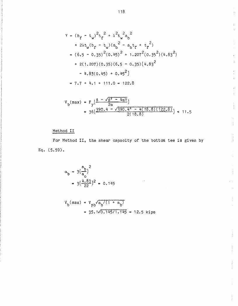
118

Y = (b - t )2t 2 + A2t 2s 2

f w f w b

+ 2Atw(bf- tw)(sb2- sbtf + tf2)

= (6.5 - 0.35) 2(0.45) 2 + 1.2072(0.35 2)(4.83 2)

+ 2(1.207)(0.35)(6.5 - 0.35)(4.83 2

- 4.83(0.45) + 0.452 )

= 7.7 + 4.1 + 111.0 = 122.8

Vb(max) = F (8 - 182 - 4aY) y 2a ·~~~--~~~~~"'

= 36(390.4- 1390.4 2 - 4(18.8)(122.8)) 11 5

2(18.8) .

Method II

For Method II, the shear capacity of the bottom tee is given by

Eq. (5.59).

a = b

0.145

Vb(max) = vpb/ab/(1 + ab)

= 35.1/0.145/1.145 = 12.5 kips

119

Top Tee Shear Capacity:

Method I

For Method I, the top tee shear capacity is given by (Eq.

(5.47). Using Eq. (5.34b), the concrete force at the high moment end

is limited to the tensile capacity of the top tee.

p smax Fytf(bf- tw)

= 36(0.45)(6.5

+ F t s y w t

- 0.35) + 36(0.35)(4.83)

= 100 + 61 = 161 kips

p Ch ~ p C = 360

.S. Pstuds = 323

< Psmax = 161 <==Controls

a = 161 .90 0.85(3)(70.5)

~ = 4 - ·~0 = 3.55 in.

The deck ribs are on 6 in. centers. With a 22 in. opening, a

minimum of 3 ribs will be above the opening. The concrete force and

location at the low moment end are obtained using Eq. (5.24) and

(5.25a).

P h- N RQ c o n

= 161 - 3( .797)(21.3) 110 kips

120

0.5Pcl ct

1 = T - t + s s 0.85f' b c e

0.5(110) = 4 - 2 + 0.85(3)(70.5) = 2.30 in.

The top tee "mechanism" capacity is given by Eq (5.47).

a a=3+2f3..2

st

= 3 + 2/3 l4~~3) 18.8

+ 2/3 (1.207)(0.35)(4.83)

+ 2(22)((6.5- 0.35) + 1.207(0.35))

2/3 + 4.83(36) l 161(3.55) - 110(2.30))

+ ~ (161 - 110)

= 94.2 + 7.1 + 289.2 + 6.3 + 2.5 = 399.3

y =

121

(Pch2 + Pcl2) (Cbf - tw)tf + ltwst)

2 F 2 + F ( P ch - P cl)

y y

= (6.5 - 0.35) 2(0.45) 2 + 1.2072(0.35) 2(4.83 2)

+ 2(1.207)(6.5- 0.35)(0.35)(4.83 2)

- 4.83(0.45) + 0.45 2)

+ 2((6.5- 0.35~6· 1.207(0.35))(161(3.55)- 110(2.30))

~ (161 2 + 1102)

2(36) 2

+ ((6.5- 0.35)(0.45) 3~ 1.207(0.35)(4.83)) (161 - 110)

= 7.7 + 4.2 + 111.0 + 116.3- 14.7 + 6.8 = 231.3

= 21.5 kips< vpt

Method II

For Method II, P0

h is limited only by Eq. (5.23).

p < p = 360 Ch- C

< P = 323 <== Controls - studs

- 323 a= 0.85{3)(70.5) = 1"80

d 4 - 1.80 = 3.10 . h = 2 ln.

122

P01

= 323- 3(.797)(21.3) = 272

0.5(272) dl = 4 - 2 + 0.85(3)(70.5)

= 2.76 in.

The maximum shear capacity is found using Eq. (5.64), (5.65), and

(5.68).

( P ch dh - P cl dl)

stV pt

= (323(3.10)- 272(2.76)) 4.83(35.1)

4.55

= 1. 48

= V (2uv + /12v 2 - 12u 2

+ 36) Vt(max) pt 2(3 + v2)

= 3 5 1

( 2 c 1. 48 l c 4 • 55 l + 1,.,..1-=-2 <'""4,....-=5-=-5 ""'2 l.--_-.,.-1 2"'<'""'1-. ""'48""2""')-+ ...,3=6 l • 2(3 + 4.55 2 )

= 21.9 kips< vpt

Total Capacity:

Method I

= 11.5 + 21.5

= 33.0 kips

Method II

Vm = Vb(max) + Vt(max)

= 12.5 + 21.9

= 34.4 kips

Strength Check:

The M/V ratio is

M - = v

Method I

2928 18.07

= 162 in.

123

The nominal capacity is given by Eq. (6.1).

v = n [ (~)3 l-1/3 v -- + 1

m M 3 ( .2!) v

m

= 33.0 [(1623) + 1] -1/3 ( 4310)3 33.0

= 23.1 kips

M = V (!::!) n n V

= 23.2(162) = 3745 in.-kips

Using Eq. ( 6. 3) and (6.2), the shear and moment capacities at

the web opening are found.

124

Shear Capacity = ~vvn

0.85(23.1)

= 19.6 > V = 18.1 ok u

Moment Capacity= $bMn

Method II

= 0.85(3745)

= 3183 > M u

Shear Capacity = 19.9 ok

Moment Capacity = 3227 ok

2928 ok

The selected section has adequate strength with an 11 x 22 in.

web opening at the span quarter point. In the event that a section

is not adequate with the required opening, several alternatives are

available to the designer, The material strengths can be increased,

the section weight or depth can be increased, or the deck configura-

tion may be changed. Although an increase in section depth will

increase the height of a story, the total depth will normally be less

than the depth obtained if utilities are routed below, rather than

through the section.

125

Deflections:

The beam deflections are calculated for construction and serv-

ice loads considering shear deformations throughout the span. The

beam is modeled as shown in Fig. 6.1b.

Before the concrete has hardened, the loads will consist of the

weight of the slab and the weight of the steel section. The load,

therefore, is

Construction load 0.041 + 0.007

= 0.048 ksf

and the uniform load on the beam, w, is

w = 0.048(8) = 0.384 kips/ft

At this stage, the beam is modeled using the properties of the

steel section only, Elements 1, 4, and 5 (Fig. 6.1b) are modeled

using Is = 843 in. 4 and AY = 7.23 in. 2. The top tee (element 2) is

modeled using It= 8.32 in. 4, At= 4.46 in. 2, andAyt = 1.69 in.2

,

while the bottom tee (element 3) is modeled using Ib = 8.32 in. 4

, Ab

= 1.69 in. 2, and Ayt = 1.69 in. 2 . The eccentricities for the top and

bottom tees are 9.27 in. and -9.27 in., respectively.

After the concrete has hardened, additional loads will include

the live load, the partition load, and the ceiling load. The addi-

tional load is

1~

Service load= 0.100 + 0.020 + 0.008 = 0.128 ksf

and the uniform load is

w = 0.128(8) 1.024 kips/ft

The beam is now modeled using the composite properties. Elements 1,

4, and 5 are modeled using Ieff = 2044 in.4

and AY = 7.23 in.2

• The

top tee is modeled using It 8.32 in. 4

, At= 18.56 in. 2, and Ayt =

1.69 in. 2• The bottom tee is modeled using Ib = 8.82 in. 4, Ab = 4.46

in. 2 , and Ayb = 1.69 in. 2• The eccentricities for elements 2 and 3

are 2.32 in. and -16.23 in., respectively.

The deflections are obtained using the general purpose finite

element program POLO-FINITE (24).

The respective increments in deflection at the point of maximum

moment are 0.614 and 0.703 in. under construction and service loads,

while the respective deflections across the opening are 0.086 and

0.095.

Comparing the deflections to the specified limits:

0.614 < 1-112 in. ok

0.703 < L/360 = 36(12)/360 = 1.20 in. ok

127

It is worthwhile to compare these deflections with those ob-

tained using a more traditional approach. Considering only flexural

deformations in the beam and ignoring the web opening, the respective

increments in deflection at the point of maximum moment are 0.59 and

0.65 in. under construction and service loads. The deflections are

close because the beam used in this example has a long span and a

short opening relative to its length. The effects of shear deforma-

tion and of the web opening on the overall deflections are,

therefore, relatively small.

Detailing:

In addition to the studs required over the opening and between

the opening and the support, studs should be placed in the four ribs

adjacent to the high moment end of the opening (d = 21

in., use 22 in.).

in., a = 22 0

The slab above the opening requires additional reinforcing.

A = 0.0025(12)T r s

= 0.0025(12)(4) 0.12in~/ft

Use #3 bars on 10 in. centers in both directions. Since a0

> d, the

transverse reinforcement should extend 22 in. on each side of the

section, and the longitudinal reinforcement should extend 22 in. on

each end of the opening.

1~

6.6 SUMMARY

Design Methods I and II allow rapid calculation of the nominal

shear and moment capacities of a composite beam with a web opening.

The nominal capacities are applied to design using LRFD procedures.

It is recommended that the designer increase the number and the

length of shear connectors, if possible, to take advantage of the

increased capacity at the opening afforded by increased shear connec

tor capacity. Additional shear connectors near the high moment end

of the opening and additional reinforcing steel in the slab are also

recommended. The stiffness method of matrix analysis is recommended

for estimating the deflections of composite beams with web openings.

A design example is provided,

7.1 SUMMARY

1~

CHAPTER 7

SUMMARY AND CONCLUSIONS

This study consists of laboratory tests and detailed analyses

leading to a comprehensive design procedure for composite beams with

web openings.

Fifteen tests to failure were carried out on composite beams

with web openings. All specimens were full scale beams with ribbed

slabs using formed steel deck. The ribs were oriented either perpen

dicular to or parallel to the steel section. The key parameters of

the study included moment-shear ratio at the opening, partial com

posite behavior, deck rib orientation, slab thickness, opening shape,

opening eccentricity, and modification of the deck over the opening.

A strength model is developed for both unreinforced and rein

forced openings and members with either solid or ribbed slabs. Three

versions of a practical strength design technique for unreinforced

openings are also presented. The strength model and the design

techniques are compared with all experimental work on composite beams

with web openings. A comprehensive design procedure, including both

strength and serviceability criteria is developed.

7.2 CONCLUSIONS

Based on the study presented in this report, the following

conclusions can be made:

130

1) The peak loads attained by composite beams with ribbed slabs

at web openings are governed by the failure of the concrete slab.

For slabs with transverse ribs, rib failure around the shear connec

tors occurs. For slabs with longitudinal ribs, a longitudinal shear

failure occurs.

2) As the number of shear connectors above the opening and

between the opening and the support increases, the failure load

increases.

3) As the ratio of moment to shear at an opening decreases,

deflections across the opening increase and transverse cracking

occurs at lower loads.

4) The failure of composite beams with ribbed slabs at web

openings is, in general, quite ductile. Failure is preceded by major

cracking in the slab, yielding of the steel, and large deflections in

the member.

5) First yield in the steel around an opening does not give an

accurate measure of the section capacity.

6) The strength of composite beams with web openings can be

calculated with reasonable accuracy using equilibrium methods. The

strength model provides an accurate prediction of the test results

from this study and from previous investigations.

7) Relatively simple strength design procedures, based on

equilibrium methods, also give a good prediction of test results.

8) The analyses using the strength model and the strength

design procedures clearly indicate the importance of considering

131

partial composite action in determining the strength of composite

beams with web openings.

9) Beam deflections can be estimated, with reasonable accuracy,

using the stiffness method of matrix analysis. The opening is modeled

as two uniform beam elements, each connected to the beam by two rigid

links. The most accurate estimates are obtained using a model which

considers shear deflections (model V). Similar results can, however,

be obtained by multiplying the deflections obtained with model V by a

correction factor.

10) The effect of a web opening on beam deflection increases as

both the shear at the opening and the relative size of the opening

increase.

7.3 FUTURE WORK

Only two composite beams with reinforced openings have been

tested (8). Additional testing, particularly of partially reinforced

openings (openings with reinforcement at only one tee), is required.

The test results can be used to confirm the accuracy of the strength

model, which accounts for reinforcement at the opening.

An extension of the current simplified design procedures which

accounts for reinforcement at the opening is required.

Stability considerations were outside the scope of this

project. While elastic buckling was not observed in any of the

reported tests of composite beams with web openings, no stability

criterion have been developed for composite beams with web openings.

132

An investigation of buckling at web openings in composite beams is

required.

The contribution of the slab to the strength of composite beams

at web openings is well documented. Additional work is required,

however, to investigate modifications of the slab that will provide

inexpensive reinforcement at the opening.

To date, no tests of adjacent openings in composite beams have

been conducted. An investigation of the interaction between adjacent

openings in composite beams is, therefore, highly desirable.

The deflection analysis of composite beams with web openings

can be simplified by the development of design aids which allow the

designer to apply factors, based on opening size and location, to the

bending deflection of a beam without an opening.

133

1. ACI, Building Code Requirements For Reinforced Concrete (ACI 318-83), American Concrete Institute, Detroit, MI, 1983, 111 pp.

2. AISC, Manual Of Steel Construction, Eighth Edition, American Institute of Steel Construction, Inc., Chicago, IL, 1980.

3. AIS C, Proposed Load And Resistance Factor Design Specification for Structural Steel Buildings, American Institute of Steel Construction, Inc., Chicago, IL, 1983, 166 pp.

4. Bjorhovde, R., and Zimmerman, T. J., "Some Aspects of StubGirder Design," Engineering Journal, AISC, Vol. 17, No. 3, 3rd Quarter, 1980, pp. 54-69.

5. British Standards Institution, BS 5400, Steel, Concrete and Composite Bridges, Part 5: Code of Practice for Design of Composite Bridges, BSI, London, 1979.

6. Buckner C. D., Deville, D. J., and McKee D. c., "Shear Strength of Slabs in Stub Girders," Journal of the Structural Division, ~. Vol. 107, No. ST2, Feb. 1981, pp. 273-280.

1. Canadian Standards Association, Steel Structures for Buildings-Limit States Design, Standard No. CAN3-S16.1-M78, CSA, Rexdale, Ontario, Dec. 1978.

8. Cho Soon Ho, "An Investigation On The Strength Of Composite Beams With Web Openings," Thesis presented to Hanyong University, Seoul, Kore·a, Dec. 1982, in partial fulfillment of the requirements for the degree of M.S. Arch. Eng., 270 pp.

9. Clawson, W. C., and Darwin, D., "Tests Of Composite Beams With Web Openings," Journal of the Structural Division, ASCE, Vol. 108, No. ST1, Jan. 1982, pp. 145-162.

10. Clawson, W. C., and Darwin, D., "Strength Of Composite Beams With Web Openings," Journal of the Structural Division, ASCE, Vol. 108, No. ST3, Mar. 1982, pp. 623-641.

11. Clawson, W. C., and Darwin, D., "Composite Beams With Web Openings," Structural Engineering and Engineering Materials SM Report No. 4, University of Kansas Center for Research, Inc., Lawrence, Kansas, Oct. 1980, 209 pp.

12. Conte, s. D., and de Boor, C., Elementary Numerical Analysis: An Algorithmic Approach, 3rd Edition, McGraw-Hill, Inc., 1980, 432 pp.

13lJ

13. Cook, R. D., _£oncepts and Applications Of Finite Element Analysis, 2nd Edition, John Wiley and Sons, New York, 1981, 537 pp.

1lJ. Darwin, D., "Composite Beams With Web Openings,"Proceedings, National Engineering Conference, American Institute of Steel Construction, Chicago, IL, March 198lJ, 17 pp. Also, Journal of the Boston Society of Civil Engineers Section, ASCE, Vol. 71, No. 1 & 2, 1985, pp. 67-83.

15. Donoghue, C. M., "Composite Beams With Web Openings: Design," Journal of the Structural Division, ASCE, Vol. 108, No. ST12, Dec. 1982, pp. 2652-2667.

16. Dougherty, B. K., "The Effects Of Rectangular Web Holes On The Behavior Of Steel Beams," thesis presented to the University of Natal, Durban, South Africa, in 1978, in partial fulfillment of the requirements for the degree of Doctor of Philosophy in Engineering.

17. Dougherty, B. K., "Elastic Deformation Of Beams With Web Openings," Journal of the Structural Division, ASCE, Vol. 106, No. ST1, Jan. 1980, pp. 301-312.

18. Fenves, s. J., Logcher, R. D., and Mauch, S.P., STRESS: A Reference Manual, A Problem-Oriented Computer Language for Structural Engineering, The Department of Civil Engineering, Massachusetts Institute of Technology, Cambridge, 1965.

19. Granade, C. J., "An Investigation Of Composite Beams Having Large Rectangular Openings In Their Webs," thesis presented to the University of Alabama, at University, Alabama, in 1968, in partial fulfillment of the requirements for the degree of Master of Science.

20. Grant, J. A., Jr., Fisher, J. W., and Slutter, R. G., "Composite Beams with Formed Steel Deck," AISC Engineering Journal, Vol. 14, No.1, First Quarter, 1977, pp 24-43.

21. Horne, M. R. Plastic Theory of Structures, The M.I.T. Press, Cambridge, Massachusetts, 1971, 173 pp.

22. Kullman, R. B., Hosain, M. u., "Shear Capacity of Stub-girders: Full Scale Tests," Journal of Structural Engineering, Vol. 111, No. 1, January, 1985, pp. 56-75.

23. Kupfer, H., Hilsdorf, H. K., and RUsch, H., "Behavior Of Concrete Under Biaxial Stress," ACI Journal, Proceedings, Vol. 66., No. 8, Aug. 1969, pp. 656-666.

135

24. Lopez, L.A., Dodds, R. H., Jr., Rehak, D. R., and Urzua, J., Polo-Finite: A Structural Mechanics System For Linear And Nonlinear Analysis, Issued as a technical report by: Civil Engineering Laboratory, University of Illinois at UrbanaChampaign and Department of Civil Engineering, University of Kansas, Lawrence, KS, 1980.

25. Logcher, R. D., et. al., ICES STRUDL-I, The Structural Design Language, Department of Civil Engineering, M.I.T., Cambridge, 1967.

26. McCormick, M. M., Open Web Beams-- Behavior, Analysis And Design, BHP Melbourne Research Laboratories Report MRL 17 I 18, Melbourne Research Laboratories, The Broken Hill Proprietary Company Limited, Clayton, Vic., Australia, Feb. 1972, 195 pp.

27. McCormick, M. M., Discussion of "Suggested Design Guides For Beams With Web Holes," Journal of the Structural Division, ASCE, Vol. 98, No. ST12, Dec. 1972, pp. 2814-2816.

28. Momeni, Ali M., "Strength Of Composite Beams With Eccentric, Reinforced, Rectangular Web Openings," thesis presented to Kansas State University, Manhattan, Kansas, in 1983, in partial fulfillment of the requirements for the degree of Doctor of Philosophy.

29. Ollgaard, J. G., Slutter, R. G., and Fisher, J. W., "Shear Strength of Stud Connectors in Lightweight and Normal-Weight Concrete," AISC Engineering Journal, Vol. 8, No. 2, April, 1971, pp 55-64.

30. Poumbouras, G., "Modification Of A Theory Predicting The Shear Strength Of Composite Beams With Large Web Openings," Project Report, No. U83-20, Department of Civil Engineering and Applied Mechanics, McGill University, Montreal, Quebec, Canada, April 1983, 109 pp.

31. Redwood, R. G., "Plastic Behavior and Design of Beams with Web Openings," Proceedings, First Canadian Structural Engineering Conference, Toronto, Canadian Steel Industries Construction Council, Toronto, Canada, Feb. 1968, pp. 127-138.

32. Redwood, R. G., and Poumbouras, G., "Tests Of Composite Beams With Web Holes," Canadian Journal of Civil Engineering, Vol. 10, No. 4, 1983, pp. 713-721.

33. Redwood, R. G., and Poumbouras, G., "Analysis Of Composite Beams With Web Openings," Journal of the Structural Engineering, ASCE, Vol. 110, No.-s1T;--sept-:-1984;-p-p-.--T"91i9= 1958.

136

34. Redwood, R. G., and Wong, P. K., "Web Holes In Composite Beams With Steel Deck," Proceedings, Eighth Canadian Structural Engineering Conference, Canadian Steel Construction Council, Willowdale, Ont., Canada, Feb. 1982, 41 pp.

35. Slutter, R. G., and Driscoll, G. C., Jr., "Flexural Strength Of Steel-Composite Beams," Journal of the Structural Division, ASCE, Vol. 91, No. ST2, Apr. 1965, pp. 71-99.

36. Steel Deck Institute, Design Manual for Floor Decks and Roof Decks, 1978.

37. Structural Investigation Of A Typical Floor Beam At The 200 West Adams Building, Chicago, Illinois, WJE No. 840795, Wiss Janney, Elstner Associates, Inc., Northbrook, IL, Aug. 1984, 21 pp.

38. "Suggested Design Guides For Beams With Web Holes,• by the Subcommittee on Beams with Web Openings of the Task Committee on Flexural Members of the Structural Division, John E. Bower, Chmn., Journal of the Structural Division, ASCE, Vol. 97, No. ST11, Nov. 1971, pp. 2702-2728.

39. "Suggested Design Guides For Beams With Web Holes,• Closure by the Subcommittee on Beams with Web Openings of the Task Committee on Flexural Members of the Structural Division, John E. Bower, Chmn., Journal of the Structural Division, ASCE, Vol. 99, No. ST6, June 1973, pp. 1312-1315.

40. Swartz, S. E., and Eliufoo, K. S., "Composite Beams With Web Openings,• Journal of the Structural Division, ASCE, Vol. 106, No. ST5, May 1980, pp. 1203-1208.

41. Thompson, P. J., and Ainsworth, I., "Composite Beams With Web Penetrations: Grosvenor Place, Sydney, Third Conference on Steel Developments, Australian Institute of Steel Construction, Melbourne, Australia, May, 1985, 18 pp.

42. Todd, D.M., and Cooper, P. B., •strength Of Composite Beams With Web Openings,• Journal of the Structural Division, ASCE, Vol. 106, No. ST2, Feb. 1980, pp. 431-444.

43. Uniform Building Code, International Conference of Building Officials, Whittier, 1985, 819 pp.

44. U.S. Steel Corp., Re.£!~!!~ular, Concentric And Eccentric Unreinforced Web Penetrations In Composite Steel Beams - A Design Aid, ADUSS 27-8532-01, Pittsburgh, Pa., Oct. 1984, 27 pp.

137

45. U.s. Steel Corp., Rectangular Concentric and Eccentric linreinforced Web Penetrations in Steel Beams - A Design Aid, ADUSS 27-7108-01, Pittsburgh, Pa., June 1981, 28 pp.

46. Wong, P. P. u., and Redwood, R. G., "Pilot Test Of A Hollow Composite Beam Containing A Web Opening," Structural Engineering Report, No. 80-6, McGill University~IMontreal, Quebec, Canada, Dec. 1980, 40 pp.

47. Yam, Lloyd C. P., Q~l£~_Of_~~~~~~!!~-~!~~l:~~~~~~!~ Structures, Surrey University Press, London, 1981, 168 pp.

138

Table 2.1 Steel Strength, ksi.

TOP FLANGE BOTTOM FLANGE Static Tensile Static Tensile

Beam Yield Yield Yield Yield

54.6 50.6 71.9 52.3 50.7 71 • 9

2 52.3 49.2 71.2 51.2 48.8 71.4

3 52.6 50.6 71.6 51.7 49.6 71.5

4 52.6 50.0 71.9 53.6 50.2 71.8

5 53. 1 50.4 72.4 54.7 49.5 72.2

6 53.6 50.8 71.7 52.7 49.7 72.4

7 40.6 38.4 68.6 41.1 38.5 68.7

8 47.6 45.0 69.4 47.7 45. 1 69.9

9 41 . 1 38.5 68.7 40.6 38.4 68.6

WEB (HORIZ.) WEB (VERT.) Static Tensile Static Tensile

Beam Yield Yield Yield Yield

55.4 51.8 72.8 55.9 53.0 73.4

2 53.1 50.7 73.5 55.5 53.2 74.2

3 52.5 50.4 73.4 54.9 53.3 74.1

4 53.7 50.7 74.1 56. 1 53.4 74.4

5 52.7 50.0 72.0 55.9 52.9 73.2

6 52.7 50.2 73.9 57.0 54.7 75.9

7 41.2 38.8 70.1 42.4 39.7 68.7

8 50.8 47.7 72. 1

9 41 . 2 38.8 70. 1 42.4 39.7 68.7

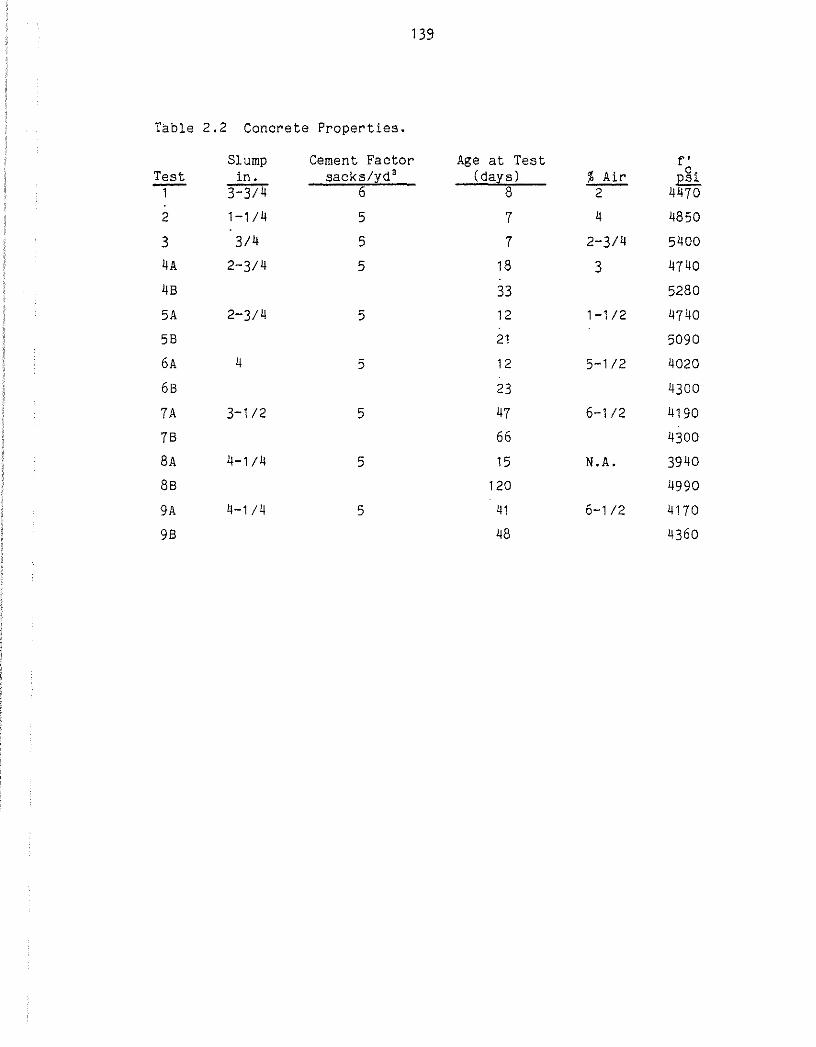
139

Table 2.2 Concrete Properties.

Slump Cement Factor Age at Test f' Test in . sacks/yd' (da;t:sl % Air pgi .,.- 3-3/4 6 8 2 4470

2 1-1/4 5 7 4 4850

3 3/4 5 7 2-3/4 5400

4A 2-3/4 5 18 3 4740

48 33 5280

5A 2-3/4 5 12 1-1/2 4740

58 21 5090

6A 4 5 12 5-1/2 4020

68 23 4300

7A 3-1/2 5 47 6-1/2 4190

7B 66 4300

8A 4-1/4 5 15 N.A. 3940

8B 120 4990

9A 4-1/4 5 41 6-1/2 4170

98 48 4360

140

Table 2.3 Section and Opening Dimensions, in.

bf(Top) tf(Top) +

Test Section d t st sb w

1 W21 X 44 20.63 6.51 0.440 0.358 4. 178 4.101 2 6.50 0.427 0.357 4. 094 4.094 3 6.57 0.423 0.358 4.105 4.097 4A 6.50 0.435 0.357 4. 1 00 4.100 4B 6.50 0.435 0.357 4. 125 4.125 5A 6.51 0.440 0.358 4.168 4. 11 0 5B 6.57 0.440 0.358 4.110 2.123 6A 6.58 0.440 0.357 4. 120 4.115 6B 6.58 0.440 0.357 4. 120 4.115 7A 6.66 0.409 0.360 4.025 4. 150 7B 6.66 0.409 0.360 4.075 4.188 8A W10 X 15 10. 13 3.98 0.268 0.231 2.090 2. 090 8B 3.98 0.268 0.231 2.025 1 • 725 9A W21 X 44 20.63 6.67 0.425 0.365 2.960 2.960 9B 6.67 0.427 0.369 3. 075 2.812

Test bf(Bot) tf(Bot) b b * t T Opening Size cone e s _s_

1 6.50 0.430 48.0 48.0 2.0 5.0 12.38 X 24.75 2 6.51 0.448 48.0 48.0 2.0 5.0 12.38 X 24.75 3 6.56 0.435 48.0 48.0 2.0 5.0 12.38 X 24.75 4A 6.57 0.440 48.0 48.0 2.0 5.0 12.38 X 24.75 4B 6.57 0.440 48.0 48.0 2.0 5.0 12.38 X 24.75 5A 6.50 0.430 48.0 48.0 2.0 5.0 12.38 X 24.75 5B 6.45 0.430 48.0 48.0 2.0 5.0 14.39 X 24.75 6A 6.57 0.432 48.0 48.0 2.0 5.0 12.38 X 24.75 6B 6.57 0.432 48.0 48.0 2.0 5.0 12.38 X 24.75 7A 6.59 0.412 48.0 48.0 2.0 5.0 12.38 X 24.75 7B 6.59 0.412 48.0 48 .o 2.0 5.0 12.38 X 24.75 8A 4.02 0.280 39.4 36.0 2.5 5.5 5.95 X 11 • 82 8B 4.02 0.280 39.4 36.0 2.5 5.5 6.38 X 18.63 9A 6.61 0.429 48.0 48.0 4.0 7.0 14.75 X 24.75 9B 6.61 0.427 48.0 48.0 4.0 7.0 1 4. 75 X 1 4, 75

+ Opening eccentricity = e e = 0 for Tests 1 through 5A, 6A through 8A, and 9A e = -1 .oo in. for Test 5B e = -0.15 in. for Test 8B e = -0. 1 3 in. for Test 9B

* b = effective slab width e

141

Table 2.4 Stud and Rib Properties.

Stud + h t tt * ** Test Diameter H w N N

3 r r 0

in. in. in. in.

1 3/4 4.5 3.0 6.0 2*2 5*2 2 2*2 5*2 + 3*4 3 2*2 10*2 4A 0*2 5*1 48 0*2 5*2 + 3*4 5A 2*1 7*1 58 2*2 8*2 6A 2*2 6*2 68 8 20 7A 1 0 22 78 6 22 8A 5/8 5.0 1 *2 4*2 88 1*2 3*2 9A 3/4 5.5 2*2 5*2 98 1*2 4*2

+ H stud height after welding s

t h = rib height r tt average rib width w = r * N no. of studs over opening -- For transverse ribs = no. of

0 ribs * of studs/rib no.

** N = no. of studs between high moment end of the opening and the

support -- For transverse ribs = no. of ribs * no. of studs/rib

142

Table 3.1 Test Behavior.

First Appearance of First Crack +

M Yield Transverse Longitudinal Diagonal v Test (ft) % Ult

+ % Ult+ % Ult+ % Ult +

1 3.50 36 44 92 67 2 6.50 32 65 80 80 3 45.20 44 96 76 81 4A 6.50 32 69 95 69 4B 6.50 19 O* 88 51 5A 6.50 31 58 93 93 5B 6.50 30 0* 47 70 6A 0.00 36 21 70 70 6B 3.50 34 0* 65 94 7A 3.50 35 40 80 N.A. 7B 6. 50 25 66 66 N. A. SA 3.30 25 93 93 93 8B 2.50 52 42 87 71 9A 3.50 27 25 91 53 9B 3.00 38 38 70 70

+ Applied Load * Crack appeared when opening was cut

Table 3.2 Test Results.

Maximum Total

Applied Load Total Load Total Load Load at Opening

Test ~ at Opening M Vat opening ~d at opening M v Failure

(ft) (ft) (in. kips) (kips) Mode

3.50 3.54 2.06 1606 47.8 Rib Failure

2 6.50 6.61 3.85 3095 39 .o Rib Failure

3 45.20 44.80 26.07 6075 11.3 Crushing at Failure

4A 6.50 6.63 3.86 2603 32.7 Rib Failure

4B 6.50 6.62 3.85 3096 39.0 Rib Failure ..,.. 5A 6.50 6.67 3.88 2768 34.6 Rib Failure "' 5B 6.50 6.65 3.87 2568 32.2 Rib Failure

6A o.oo 0.00 o.oo o.o 41 .o Rib Failure

6B 3.50 3.53 2.05 2070 48.9 Rib Failure-Diag. Tension

7A 3.50 3.53 2.05 1845 43.5 Long. Shear

7B 6.50 . 6.61 3.85 3379 42.6 Long. Shear

8A 3.28 3.32 3.93 774 19.4 Rib Failure-Diag. Tension

8B 2.45 2.49 2.95 427 14.3 Rib Failure-Diag. Tension

9A 3.50 3.56 2.07 1474 34.5 Rib Failure

9B 3.00 3. 13 1.82 1775 47.3 Rib Failure

144

Table 3.3 Relative Deflection at Failure.

Applied M * + -t v 0 0 0 m 0

Test (ft) (in.) (in.)

1 3.50 0.72 0. 77 1.07 2 6;50 0;74 0.60 0.81 3 45.20 4.00 0.1 0 0;03 4A 6.50 0.58 0. 71 1 .22 4B 6.50 1. 31 1.27 0.97 5A 6.50 1.95 1.88 0.96 5B 6.50 1.04 1.26 1 • 21 6A 0.00 1.05 2.38 2.27 6B 3.50 1.36 1. 43 1.05 7A 3.50 0.88 0.82 0.93 7B 6.50 0.99 0.51 0.52 SA 3.30 0.61 0.42 0.69 8B 2.50 0.55 0.70 1.27 9A 3.50 0.96 1. 61 1. 68 9B 3. 00 0.98 1.27 1.30

* 0 Deflection at point of maximum moment. m

+ 0 0

Deflection across web opening.

t 0 = o lo o m

145

Table 4.1 Ratios of Test to Calculated Strength for the Strength Model.

Test Test

t Test Shear Moment Test/Theory

kips in.-kips Ratio Testt Shear Moment Test/Theory kips in.-kips Ratio

1 37. 8 2 39.0 3 11.3 4A 32.7 4B 39.0 5A 34.6 58 32.2 6A 41.0 6B 48.9 7A 43.5 7B 42.6 8A 19.4 8B 14.3 9A 34.5 9B * 47.3 Mean * Std. Dev.

RO 18.2 R1 26.0 R2 28.7 R3 16. 4 R4 13.1 R5 27.6 R6 21.2 R7 30.5 R8 28.9 Mean Std. Dev.

1606.0 3095.0 6075.0 2603.0 3096.0 2768.0 2568.0

0.0 2070.0 1845.0 3379.0

774.0 427.0

1474.0 1755.0

752.0 978.0

2904.0 3993.0 3212.0 1038.0 786.0

1134.0 1075.0

Ribbed slab summary:

* Mean * Std. Dev.

t G- Granade (19)

0.919 0.993 1. 060 1.128 1. 314 0.949 0.995 1. 118 1. 027 1. 092 1. 128 0.942 0.947 0.962 1. 006 1. 011 0.070

0.904 1. 059 1. 089 1. 135 1. 102 0.995 1. 076 1. 001 1. 001 1. 040 0.071

1. 023 0.070

C- Clawson and Darwin (9, 11) CHO - Cho (8) R - McGill Tests (32, 34)

C1 C2 C3 C4 C5 C6 G1 G2 Mean Std. Dev.

CH03 CH04 CH05 CH06 CH07 Mean Std. Dev.

33.4 36.8 14.0 47.6 48. 1 40.4 32.7 26.5

35.7 46.7 17.9 40.6 20.6

2886.0 4107.0 5468.0 1723.0 3511.0 1471.0 791.0

1 296. 0

634.0 1477.0 2319.0 721.0

2664.0

Solid slab summary:

Mean Std. Dev.

Overall summary:

* Mean Std. Dev.*

* Tests 4A and 4B excluded from calculations.

1. 095 1. 114 1. 118 1.093 1. 129 1. 079 1 . 164 1. 018 1 . 101 0.043

1. 126 0.999 1. 013 1. 064 0.960 1. 032 0.064

1.074 0.060

1.042 0.071

146

Table 5. 1 Ratios of Test to Calculated Strength for the Redwood and Poumbouras (33) Procedure, the Strength Model (Chapter 4), and Strength Design Methods I, II, and III.

Test/Theory Ratio Test Redwood-

Test Shear Moment Poumbouras Design Method IF kips in.-kips Procedure Model I II III

1 37.8 1606.0 0.895 0.919 0.968 0.913 0.967 2 39.0 3095.0 0.986 0.993 1. 053 1.026 1. 080 3 11.3 6075.0 1. 014 1. 060 1. 027 1. 027 1. 028 4A 32.7 2603.0 1. 046 1. 128 1. 157 1. 083 1 • 1 32 48 39.0 3096.0 1. 212 1 . 31 4 1.360 1. 238 1. 298 5A 34.6 2768.0 0.919 0.949 1. 009 0.960 1. 009 58 32.2 2568.0 0.977 0.995 1. 058 1. 020 1. 074 6A 41.0 0.0 1.137 1. 118 1.135 1. 132 1 • 199 6B 48.9 2070.0 1. 016 1. 027 1. 080 1.044 1. 093 7A 43.5 1845.0 0.984 1. 092 1.035 1. 000 1. 005 7B 42.6 3379.0 1. 030 1. 128 1.093 1. 087 1. 097 8A 19.4 774.0 1. 081 0.942 0.971 0.985 0.990 8B 14.3 427.0 0.918 0.947 0.926 0.934 0.928 9A 34.5 1474.0 1 . 116 0. 962 0.937 0.976 o. 973 9B

* 47.3 1755.0 1. 362 1. 006 0.987 1 • 0 11 1. 018 -- --Mean *

1. 033 1 • 011 1. 021 1.009 1. 035 Std. Dev. 0.123 0.070 0.063 0.059 o. 072

RO 18.2 752.0 0.976 0.904 o. 941 0.950 0.955 R1 26.0 978.0 1. 090 1. 059 1. 100 1. 114 1. 163 R2 28.7 2904.0 1. 234 1. 089 1 • 191 1. 326 1.384 R3 16.4 3993.0 1. 126 1. 135 1. 080 1. 084 1. 084 R4 1 3. 1 3212.0 1. 068 1. 102 1. 118 1. 113 1. 118 R5 27.6 1038.0 1 • 171 0.995 1. 031 1. 040 1. 081 R6 21.2 786.0 1. 111 1. 076 1. 127 1. 124 1 • 191 R7 30.5 11 34.0 1.017 1. 001 1. 022 1. 043 1. 040 R8 28.9 1075.0 1. 091 1. 001 1. 015 1. 092 1. 098 Mean 1.098 1. 040 1. 069 1. 098 1. 124 Std. Dev. 0.077 0.071 0.075 0. 101 o. 119

Ribbed slab summary:

* Mean *

1. 060 1. 023 1. 041 1. 045 1. 072 Std. Dev. o. 109 0.070 0.070 0.089 0.102

*Tests 4A and 4B excluded from calculations.

147

Table 5.1 Continued.

Test/Theory Ratio Test Redwood-

Test Shear Moment Poumbouras Design Method IF kips in.-kips Procedure Model I II III --C1 33.4 2886.0 1. 417 1. 095 1. 143 1. 187 1. 192 C2 36.8 4107.0 1. 115 1. 114 1. 138 1. 123 1. 128 C3 14.0 5468.0 1. 156 1 • 118 1 • 1 39 1. 139 1. 139 C4 47.6 1723.0 1. 037 1. 093 1. 056 1. 051 1. 056 C5 48.1 3511 • 0 1. 087 1. 129 1. 127 1. 128 1 • 1 34 C6 40.4 1 471 • 0 1. 294 1. 079 1. 055 1. 122 1. 128 G1 32.7 791 • 0 1. 865 1 . 164 1.198 1. 284 1. 300 02 26.5 1296.0 1. 511 1. 018 1. 087 1 • 1 43 1. 153 Mean 1. 310 1 • 101 m 1.147 1 • 154 Std. Dev. 0.279 0.043 0.049 0.067 0.070

CH03 35.7 634.0 2.573 1. 126 1.160 1 • 191 1. 199 CH04 46.7 1477.0 1. 513 0.999 1. 064 1. 061 1. 071 CH05 17.9 2319.0 1. 019 1. 01 3 0.978 0.978 0.979 CH06 40.6 721.0 2.856 1. 064 1. 276 1. 311 1. 320 CH07 20.6 2664.0 1. 046 0.960 0.954 0.958 o. 959 --Mean 1. 801 1. 032 1. 086 1. 100 1. 106 Std. Dev. 0.862 0.064 0.133 0.149 0.153

Solid slab summary:

Mean 1. 499 1. 07 4 1. 105 1 • 1 29 1. 135 Std. Dev. 0.596 0.060 0.087 0. 103 0.106

Overall summary:

* Mean 1. 223 1. 042 1. 065 1. 076 1. 095 Std. Dev.* 0.423 0.071 0.082 o. 102 0.106

* Tests 4A and 4B excluded from calculations.

148

Table 5.2 Ratios of Test to Calculated Strength for the Redwood and Poumbouras (33) Procedure.

Published Calculated Calculated Test Ratios (33) Ratios* Ratios**

RO 0.995 0.976 0.976 R1 1. 129 1 • 1 31 1. 090 R2 1.163 1. 158 1. 234 R3 1. 126 1. 126 1. 126 R4 1. 108 1. 095 1. 068 R5 1. 169 1 . 171 1 • 171 R6 1. 116 1. 112 1. 111 R7 1. 017 1. 014 1 .017 R8 1. 098 1. 091 1 • 091 Mean 1. 102 1. 097 1. 098 Std. Dev. 0.060 0.064 0.077

* Based on stud capacities from pushout tests (30, 32, 34, 46). ** Based on stud capacities calculated using E = 5000/f' MPa. c c

tn 0.

.... I c -' ..,

c:

!

0.8

0.6

... ... E

' 0.4 E

0.2

149

0.2 V/Vp

Bean 2

Beam 1

Fig. 1.1 Comparison of Todd-Cooper Model wit~ Granade's Beams (42).

4000r-------r------,------~-------.------.-------,

3000

.._____ Sl111>llfled ElliPtical Interaction ---Strength Model~~

2000

1000

OL-----~------~----~------~----~~----~ 0 10 20 30 40 50 60

Shear, kips

Fig. 1.2 Full Strength Model and Simplified Moment~Shear Interaction Diagrams for Clawson and Darwin (10, 11).

150

l1mt-------LFull COI!1lOSite Action ----/<~Portio! COI11loslte Action

M'l-------------------~----~·~ ...., ~'~mr '

! 01 c ~ 111~-------------------------;

~

v., Shear

Fig. 1.3 Moment-Shea!" Intel"action Diagl"am fo!" Redwood and Poumbou!"as (33).

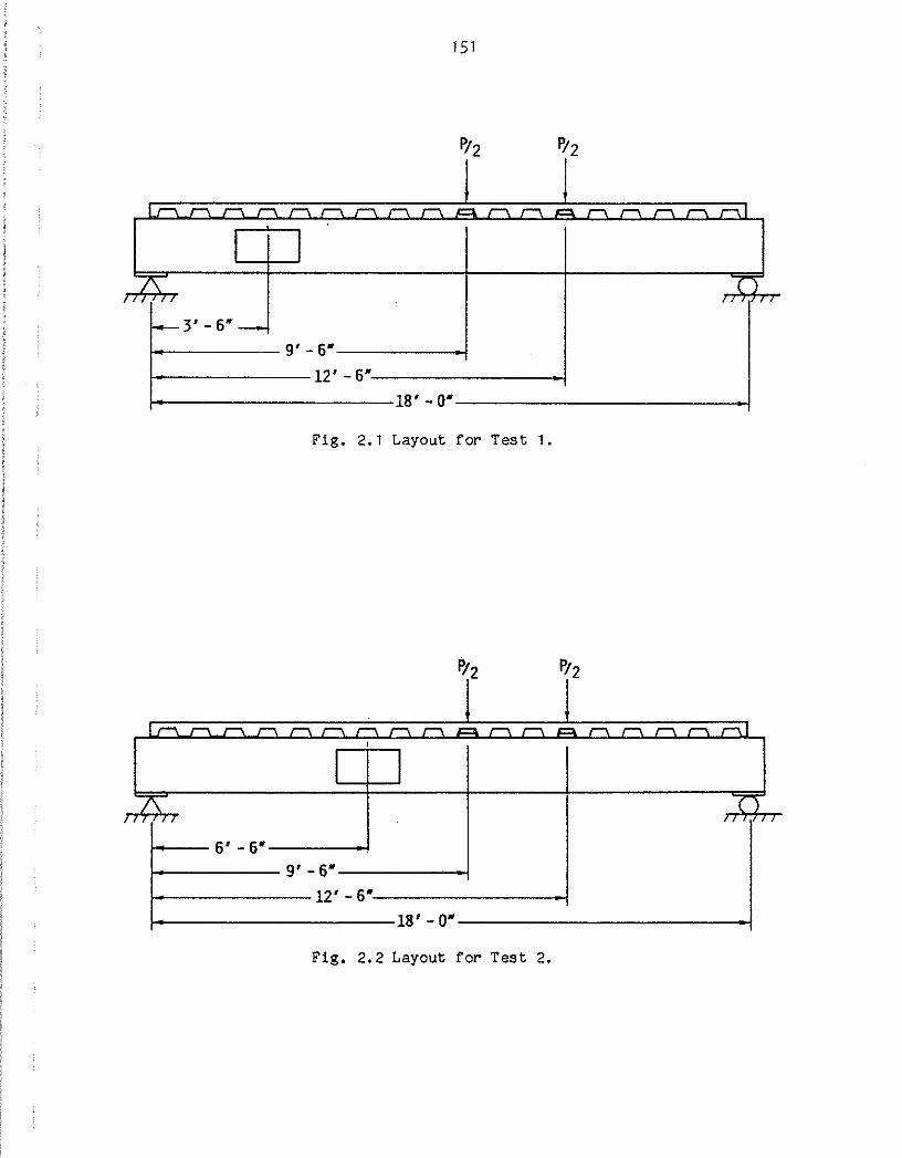
151

Lr-\ J\ . r-.. r-.. r-.. ,..-.. r-.. r-.. ,-.. .c=. r-.. ,..-.. c:o. r-.. ,...... ,...... r-. ,...;.. I

I I 7\ TI

Ill I I ' r---3' -6"-

9'- 5•

12' - 5•

18'- o·

Fig. 2.1 Layout for Test 1.

L.r-\. .r-\ r ""\ r '"\ ,..-.. ,..-.. ,..-.. r-.. r ""\ .c=. ,..-.. ,..-.. c:o. r-.. ,--. ,--. r-\ ,--. I '

I I ?- T)

I ' ' ' 6'- 5•

9'- 5•

12' - 5•

18'- o•


152

I ~ r-1 r-1 r-1 1\ 1=\ r\ 1\ r\ r\ .r-1 C\ J1 1\ 1\ 1\ r-1 r--1 ~ r--1 I I

I I 7\ u

Ill 'II "' ' f I

5'..: 6'"

a•- 5•

u· -5•

20' - o·


p

I : .I

Opening A Opening B 6'- 5• I ' 6'- 6"'

: I 9'- 5•

19' - o• Fig. 2.4 Layout for Tests 4A, 4B, 5A, and 5B.

153

I,_, """" ,..... ,......, ,......, - ,......, ~ ~ ....., ~ ~ ~ ~ ~ r-'\ ....... .,.1 I

I I rr 7\

. ' ' 5'- 6.

.I 9'- 6. 14'- 6•

17'- 6•

Fig. 2.5 Layout for Test 6A.

a Deck Pons p

I """ """ """ .Gil\ -. r--\ ~ ,--.. r-\ r-\ r-\ ,....-.. ,--.. ,--.. ,--.. ,--.. r--.. ,--.. I

I I 71 T>

' " .,

-3'-6·-6'-6·-

18'- o· Fig. 2.6 Layout for Test 6B.

154

I -1 ,... .,

I I I I I I l.. ·- "

7\ ._Opening A ~Opening B TI '"~"I "'

-3'-6"-

8'- 6" 6'- 6" 11,- 6"

~----------------------------22'-0"~--------------------------------~

Fig. 2.7 Layout for Test 7A and 7B.

p

..., r-\ ""' ,....., ,....., ,..., ,...

L [ J 1\ c

" " 3'- 3/8"-

': 5' " 0'-----l•l ~t:==~---------------12'-0"--------------~ Fig. 2.8 Layout for Test 8A.

155

p

.... r-\ r-\ ,...., ,...., ~,......~,..,

I I I

7\. ~

-2'-5~-

I -5'-0" 12' - o·


p

Opening A Opening B

3' -6" 3' -o·j - 8' -6"------1

~----------------------17'-0"----------------------~

Fig. 2.10 Layout for Tests 9A and 98.

156

f 15 11

216

._____ _ ____,_j_ Fig. 2.11 Deck Inaerta.

1------ 12. ------l

~------------24·-------------~

Fig. 2.12 Deck Profile (United Steel Deck).

IC I (

r

m.

157

• •

•

====

~ g -u...

~-_.1

•

. . •

• •

•

•

•

0

0

•

L-

'

•

t:31LF=~.!.-. --= •r--...l.F •

• •

~ . "'

158

Fig. 3.1 Failure at Web Opening with Low M/V Ratio.

Fig. 3.2 Failure at Web Opening with High M/V Ratio.

159

100

1 2 3

Ul c. .... ""' ,j Ill 0 50 _J

"0 <U

P~2 Pi2 .... ....

' J c. D c.

< I I 2 3

0

0.0 1.0 2.0 3.0

Deflection, in.

Fig, 3.3 Load-Deflection Curves for Test 1.

100

1 Ul c. .... ""' ,j Ill 50 0 _J

"0 <U ..... .... c. c. < '

pr Pi2

J D I I l 2 3

0

0.0 1.0 2.0 3.0

Deflection, in.

Fig. 3.4 Load-Deflection Curves for Test 2.

160

(II c. ....

100 ~

-.::i ttl 0

....1 P/2 P12 'C I

J Cll 50 ( CJ .... .....

I I 0. c. I 2 3 <

0~--------------------~----------------~-4 0.0 1.0 2.0 3.0 4.0 5.0 6.0

Deflection, in.

Fig. 3.5 Load-Deflection Curves for Teat 3.

100 r-------------4---------------------------~

3 2

p

: J I I I 2

0 ~------------~---------------------------4 -1.0 0.0 1.0 2.0

Deflect ion, in.

Fig. 3.6 Load-Deflection Curves for Teat 4A.

161

100~--------------~--------~-----------.

3 2 Ill Q. 1 .,., -"

-d CD 0 50 -' "0 Cll ..... ..... Q. Q.

<

p

( : J D I I I 2

0

0.0 1.0 2.0 3.0

Deflection, in.

Fig, 3.7 Load-Deflection Curves for Teat qa,

100r---------------~---------------------.

Ill Q. ..... 1 -" 2

-d CD 50 0 -' "0 Cll ..... .... Q. Q.

< D

p

: I I I 2

OL-------------------------------------4 0.0 1.0 2.0 3.0

Deflection. in. Fig. 3.8 Load-Deflection Curves for Teat SA.

162

100~--------------------------------------T

UJ 0. ..... :.e.

-o co 3 0 50 ..J

"C Gl p .....

: ..... 0. ( J 0. CJ <

I I I 2 3

OL-------------------------------------~ 0.0 1.0 2.0 3.0

Deflection, in.

Fig. 3.9 Load-Deflection Curves for Test 58.

150

1 4 3

UJ 0. .... :.e. 100

"C co 0 ..J

"C Gl

P~2 pr, ..... 50 ..... 0. h D c. < ! I A

3 2 I 4

0

-1.0 0.0 1.0 2.0

Def leoti on, in.

Fig, 3.10 Load-Deflection Curves for Test 5A.

163

100 r-----------------------------------------~

Ul 1 c. .... ..><:

• "0

"' 50 0 ....1

"0 p IIJ

: .... .....

h J c. D c. < t I

1 2

0~------------~------------------------~ -1.0 0.0 1.0 2.0

Deflection, in.

Fig. 3.11 Load-Deflection Curves tor Test 68.

100r---------------------------------------~

Ul 2 c. ....

..><:

-a "' 50 0

....1

"0 P/2 P/2 IIJ I

: .... ..... ( J c. CJ c. < I I

I 2 3

0

0.0 1.0 2.0 3.0

Deflection, in.

Fig. 3.12 Load~Detlection Curves !'or Test 7A.

IJ) a. .....

:>1'.

-o Ill 0 .J

"0 Q) .... ..... a. a. <

IJ) a. ....

:>1'.

-o Ill 0 .J

"0 Q) .... ..... a. a. <

164

100r---------------------------------------~

50

pr T J ( D

I I z 3

0 ~-----------------------------------------4 0.0 1.0 2.0 3.0

Deflection, in.

Fig. 3.13 Load-Deflection Curves for Test 7B.

50r----------------------------------------;

2

25

p

: J ( CJ I I 1 2

0 ~-----------------------------------------4 0.0 1.0

Deflection, in.

Fig. 3.14 Load-Deflection Curves for Test 8A.

2.0

165

30r-------------------------~------------~

1 fll 0. .... 2 .>1.

..a Ill 15 0 ...J

"t:l p cu

: .... ....

h J 0. D 0. < t I

1 2

0

-1.0 0.0 1.0 2.0

Deflect ion, in.

Fig. 3. 15 Load-Deflection Curves for Test 8B.

100 r-----------------------------------------~

fll 0.

2 .... 1 .>1.

..a Ill 50 0 ...J

"t:l cu p .... .... 0. 0. <

D : t I 1 2

0 ~------------...l----------------------------4 -1.0 0.0 1.0 2.0

Deflection, in.

Fig. 3.16 Load-Deflection Curves for Test 9A.

166

100

1

Ul c. ..... -"

'1:1 Ill a 50 _, '1:1 QJ p .....

: ..... ( J c.

D c. < I I

1 2

0

-LO 0.0 1.0 2.0

Deflection, in.

Fig. 3.17 Load-Deflection Curves for Test 9B.

-B -158 r I

1~~ -162~

-687 Low High 859

9~ 611

Jntcrostrotn

-210 r

9llb -4230

~~~

-1132

I I -525

"""' ' 29.8 kips 379

-618 I

-1210h Low High

I J Late Yield 88.1 kips

15800

-46,

1874

-18 r

m1 -1230

~1 -209

-154 r

1226~

>11450

Low High

~-- .. I First Yield 48.0 kips

Low High

-235 I

-329h 1681

l mlcrostroln

-547 I

-1792t

21800

18~ CJ -12,

-1588 Collapse 2620

92.5 kips

Fig. 3.18 Strain Distributions at the Opening for Test 1.

"' ......

29 -11~ ,__60 -1'fJ 52h -9~~

-Jll2 Low High 486

~ 52

11lcrostrotn

10~

"'h--1300 1mh

-188\ 1- I 158

Elastic 15.7 kips

-sa_ U-789

lBOOh 15500 Low High 15000

>20000

~ -1007

I I ~t Late Yield 93.0 kips

31b,._158

m~ -821 Low High

~ 55

L118o

3600h

[----m J

First Yield 31.5 kips

-35500 Low High

-228 "'l-30 -ml

1700

-5\ 589

lllcrostrotn

-772 -10000

-3900~

>20000

~ CJ-, -1850 Collapse 11550

97.0 kips


"' (X)

-90 -n& -180 -288

D-m -mD D-27o -2880

-34, -198l rn -198\

12 Low High 235 -20 Low High 'SOil

619 258 ~2582 ~~ ~ I I ~ CJ 893 837

402 Elastic 433 First Yield 31.9 kips 64.0 kips

JRtcrostroln Mlcrostroln

-568 -844 -1180 -2515 17..160 -432\J r -16~'0

"' r57 -44l rm h

lO

463 Low High 3159 227 Low High 15000

§ I I § § CJ § >5000 Late Yield >5000 >10000 Collapse >15000

122.5 kips 141.8 kips


29 -219 "' -316

b. -161 ""'1.55 b. -235 "1.92

mh -292h mh -516h

-848 Low High 680 -1q20 Low High 1190

1440 -617 2600 -1100

~ I I \ ~ I I \ -12 Elastic 531 -11 First Yield 852

20.0 kips 29.9 kips

Mlcrostroln Mlcrostroln

n -398 -10 -q82

~-m ""'1.88 l::::..qzo I " 0

795h -1220l 6890~ 13 -ll070 Low High 6280 Low High >30000

10300 -2870 >30000 -35200

1 CJ 1 ~ CJ 1 -333 Late Yield 1q50 .zq8o Collapse q520

50.0 kips 62.7 kips

Fig. 3.21 Strain Distributions at the Opening for Test ~A.

40 -109 110 -251 'h-88 ""110 "'h-200 "!.54

61~ -109h 18l

-303h

-m Low High 454 -717 Low High 1310

496 -210 3370 -606

~ I I \ 1 I I \ 26 Elastic 237 -24 First Yield 525

10.0 kips 20.0 kips

adcrostroln 111tcrostrotn

243 -546 138 -872 "b..-580 """'t 124 ~-mo ""l191

-...!

8ll -ll80h. l780h -4680h

-2630 Low High 9670 '

20000 Low High >20000

11700 -2740 >30000 -25700

~ CJ ' ~ I I 1 -494

Late Yield 1550 -1970 Collapse 15300

50.0 kips 74.5 kips

Fig. 3.22 Strain Distributions at the Opening for Test ~B.

37

"b:97 63h -397

~ 62

atcrostroln

~0

1':.-u~

6~~

-34~

Low High r u - - I

low

Elastic 15.0 kips

High

-146 -11'1 -128h

596

-20\ 3~

-~37

-mLJ

-1040h

4190

I~ CJ -21,

-260 lale Yield 1840

55.0 kips

38

b..-219

IBl -947 low High

-281

-~

-366h 1730

31 CJ -62\

52 First Yield 725

29.9 kips

88

l:::...-2400

1200~

-16900 low High

~ -1120

[ --1 Collapse 64.3 kips

mtcrostratn

-449 '\,.12~

-2120~

17~

-77\ 4940

Fig. 3.23 Strain Distributions at the Opening for Test 5A.

" N

63

'""h.-68

70h

-518 Low High

56~ 84

RJlcrostroln

n L11&

an~ -7380

l J

Low

Elastic 11.7 kips

High

-75 -44'\J -mh

511

-1\ 284

-961 -iN

-1220h

12500

11 CJ -3\ -m Late Yield 2000

50.1 kips

3 L84

328h

-1720

34~ 74

94

\-62

Low High

I nj First Yield

30 kips

moh >40000 Low High

-280

-151'\J

-563h 2890

-8\ 827

mlcrostroln

-921

-nN

-31SOh >40000

3~ CJ -, -1280 Collapse 4730

62.5 kips

Fig. 3.24 Strain Distributions at the Opening for Test 5B.

.__, VJ

-35 53.J'

171~ -695 Low High

-127 ""Ln

-122h

823

89~ I ~-~ -216

atcrostroln

16 Lm

1420b

-19180 Low

Elastic 31.1 kips

185

-1040 -331]

-1J90~

High 18100

~~ I ,-1~ -2090 Late Yield

119.3 kips

1930

-49 -225 52_f -2;;:1

5121 -J63h

-1660 Low High 2120

2~ I 1-1~ -549

65 Lm

3610h


-45400 Low High

485

Rllcrostrotn

-1070 -21;;:1 -moh

31000

~ I 1-3~ -3830 Collapse 4750

135.1 kips


..._, ..,..

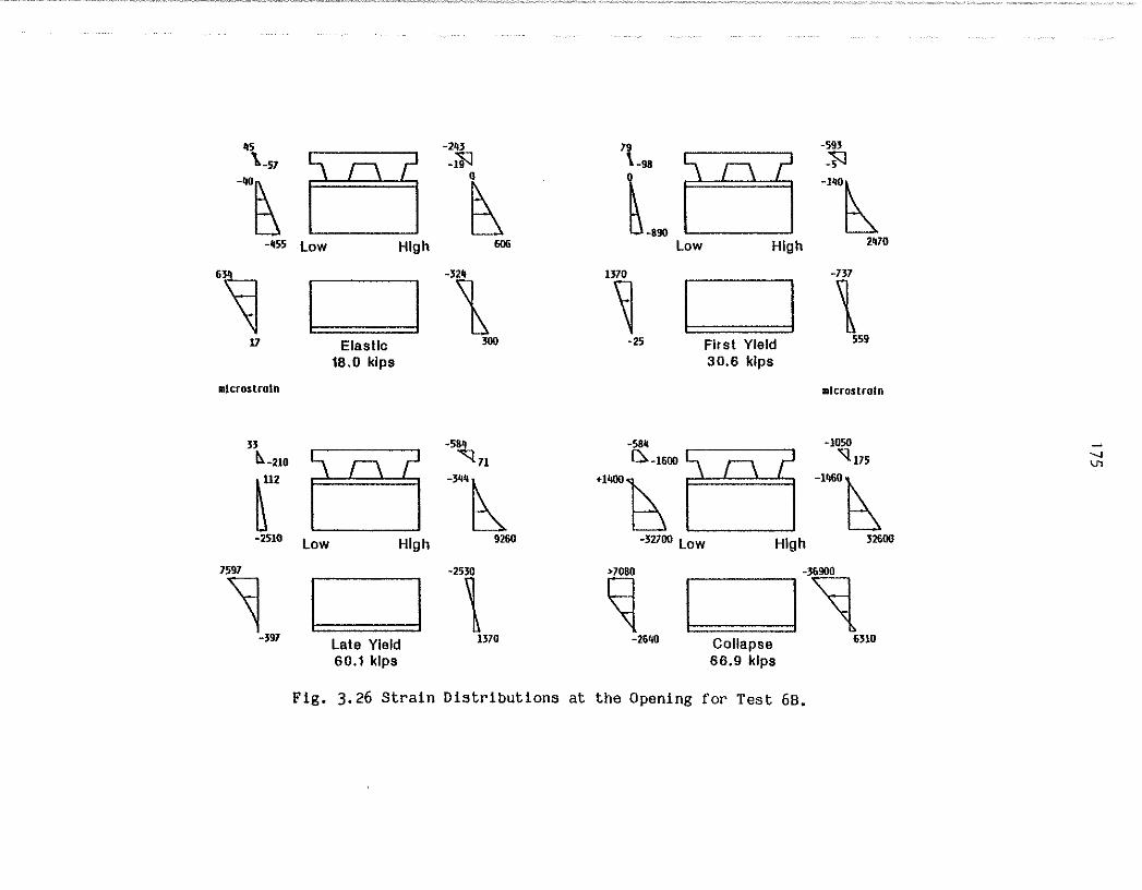
~5

\-57

-40~

-~55 Low High

6~ v

mlcrostroln

7597

33 b.-210

r -2510

1 -397

I I

Low

Elastic 18.0 kips

High

I .... ___ 1

Late Yield 60.1 kips

-243 _ifJ

0

~ 606

-3\ 300

-584

""l.n

-344l 9260

-251 1310

19 \-98

~-890 Low High

B~ -25

-5M

D.-1600

•1400~

I I First Yield 30.6 kips

-32100 Low High

-593

J:J -140~

2410

-, 559

111crostroln

-1050

"1.115

-1460h

32600

~ I ~-~ -2640 Collapse

66.9 kips

6310


" \.n

-25'1 Low High

'1 •tcrostroln

0

239111-:

~132 -1510

6~ -258

r ·-J

Low

Elastic 14.8 kips

High

r-- --J late Yield 59.8 kips

::~ -101 h

369

-1\ 201

_:::L ~6

3110

-141 1050

-68 :~201

-635

~

L:' ~

Low High

l . . .. . I First Yield 30.0 kips

-12100 Low High

~::] -319 h

677

-458

1 443

mtcrostroln

-~~ -867 ~

12100

14~ I I -68~ -997 Collapse 2450

73.8 kips


...., "'

-21 -99 -n -203

~· ------------

-~ r ----------- '1 ~0 -83 -391

-1!10 Low High 300 -430 Low High sn

~49 -59 2880 -179

~ I I h 1 I I l 97 Elastic 250 346 First Yield 517

15.0 kips 30.0 kips

atcrostroln mlcrostrotn

f' t -48~

----------- ----------- .__, .\ .__, 36 60 -1700

-2020 Low High 42~0 >6000 Low High 12100

10600 -1480 18900 -3510

~ I I \ "1 I I l 115 Late Yield 576 -206 Collapse 6510

74.8 kips 90.8 kips


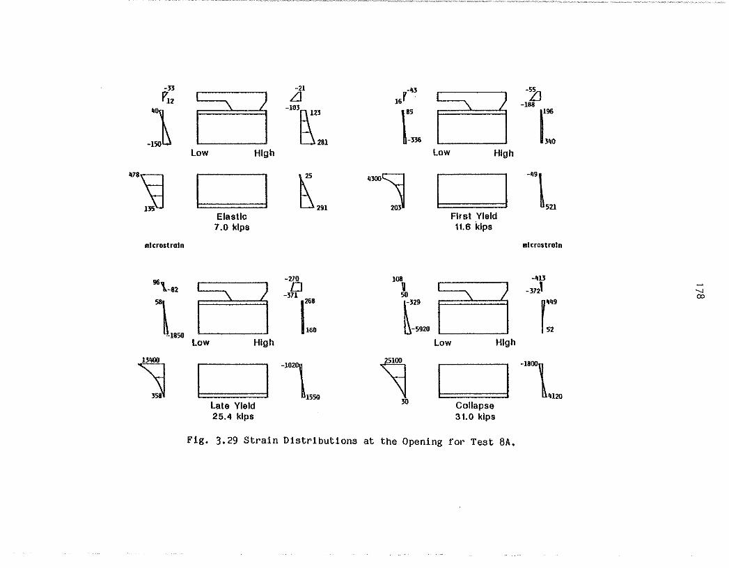
-33

rl2

_:1 ~78'\==l

1~

mlcrostrotn

96\-az

~L~

1

l \. )

low High

r-------,

Low

Elastic 7.0 kips

-"' ]

High

I n I late Yield 25.4 kips

-21

Ll -103[:\.123

lj281

l\5

~291

-270 CJ

-3711268

160

-1021

15~

-43 16r · 1 --\ )

\

85

-336

4300~

20~

Low High

I J First Yield 11.6 kips

1081329 ::>~~

~-5920 low High

~ r·-- ·· 1

30 Collapse 31.0 kips


-~ -188

l196

1340

-49\

521

mlcrostroln

-4B

-m1

r449

52

-1800\

U20

....., ():)

-llB I

70~

-3l0

~05

~ 89

rntcrostroln

0 I

12~~

-3600

>1~

-515

Low High

,- uunm I

Low

Elastic 6.2 kips

High

[--~~-n~

Late Yield 20.1 kips

-87 I

-lOb 528

-92

1

-3l8 I -10

2l0

t;: >10~

-2960

1 1380

0 I

lW~

-970 Low High

-231 I

-lOb 2660

1~ c:::J -ll\ 5~ First Yield 511

12.7 kips

0 I

~1 -UOO Low High

llltrostroln

-321 I

-10~

>15000

-~lOU

·~ c:::J t -1~ Collapse

22,9 kips


...., lO

sqg "'l.u

59~

-367

q~ -12

1dcrostroln

0 L.759

12ID1

-3990

~~ -1610

low High

-93

\29

-71h 861

-221\ .--1 II 210

Elastic 16.3 .kips

low High

~-······ ---···-·1 late Yield 54.5 kips

-'tlfl

"\tsq

-1160h lSSOO

-606~

1720

2790 "l.1so

2001 -770 Low High

-182 I 83

-208h IDIO

1~ CJ 6' -m First Yield 39q

24.3 kips

0 L.m

qo10~

-25200 Low High

mlcrostroln

-398

-1~

-3000~

>25000

·~ CJ-~ -3740 Collapse eoqo

65.1 kips


00 0

15 ~

-37

~ -358

~ -9

mtcrostroln

-55 D..

-218

~2

low High

I . . . I Elastic

16.9 kips

-~3

"'q3

~ -2~

\ -215

-209

't61

470

~ -9020 low High 15200

16700

~ -10~0

-1noo

1.------.1 1 late Yield 79.1 kips

2290

42 b.

-104

~ -933 low High

1370

~ I . I -98

-62

~m

~0


-37900 low High

-1~2

'""'!..55

~ 1410

-7\ 458

IAitrostroln

-186

"""1.32

~ 45200

37900

1 I 1-36~ -1200 Collapse

89.3 kips

8890


co

182

Fig. 3.33 Cracking in the Slab Above the Opening.

Fig. 3.34 Longitudinal Rib Failure.

183

Fig. 3.35 Rib Failure in Slab with Transverse Ribs •

• Fig. 3.36 Bridging of Slab at Opening.

1.40...------------.----------s

E :::::E '-... 0.70 '+I'

(/)

~ c

:::::E

13

e

M (test)/M - 0.3231n(M/(Vd)) + 0.137 n m r- 0.944

0.00'-------------'-----------' 0.00 1.75 3.50

ln(M/(Vd)) Fig. 3.37 M (test)/M versus ln(M/Vd) for the Current Tests and for n m Previous Investigations (8, 9, 11, 19, 32, 3~. and 36)

~

00 ..,.

1

1

1

1

1

1

1

i 1

1

Fig. 4.1 Pure Bending Failure at Opening (10, 11). 1

1

i 1

1

1

1

1

1

1

1

1

1

' I 1

1

1

1 I

( v (1> .· A

)o 6

1 M-2Vao

\ Low Moment

End Vt

<l:<:~

0 0

Mt,

vb

Mbl' I

a ()

• Co

• . I

I I I

~

0

186

. \) . 0 " 0

<l· "

Cl 0

fo ao .

q •• <;) . D

() . a " <)

ao

0 c

• 0 0

I I

I

I) Cl <:> 0

. C> .<:;:, v

\ 0 . I>

d M}2vao

High Moment End

v .q 0

t ' b • ~ .

N(h

z

vb

· Mbh I

Fig. 4.3 Forces Acting at Web Opening (10, 11).

187

J. - y I -=

= - \ -

Fig. 4. 4 "Mechanism" Failure in Pure Shear ( 10, 11).

y

I =

Fig. 4.5 "Shear" Failure in Top Tee (14).

188

--- i3p = - 190 l<p/cm2 ( 2700 psi ) PP ~p=- 315 kp/cm2 ( 4450psi) - ~p=- 590 kptcm2 ( SJSO psi) -0.20-~

I - -OJS- -I Tensile sPitting strerlgth

6;:-0lOJ op Si=-0.20461

.i ---s;...ac69 6"z 7_"'""' ~d- ---~--~

._ __ r<-:

__,...- -........ - :g_ 2 6"z "'-,. -~ :::::-- ......

~ :::--. <>- fl\ ~ :::::-- -.....(, §.. a. .-J10 0.9 o.a 0.7 0.6 o.s 0.4 0.3 0.2 0.1 -0.1

I I I I I I I I I I I Fig. 4.6 Experimental Results for the Strength of Concrete Under

Combined Tension and Compression (23) •

• 20

• 15

• 10

.05

I -0.2 0 0.2 0.4

O/f~ 0.6 0.8 1.0

Fig. 4.7 Concrete Strength Under Combined Shear and Normal Stress ( 10, 11).

-i Ill ....

j_ "' lt

.Q ....

T

-~~

189

r-

..c en

--

..... .Q

1-'-

. bO ..... c..

Fywr Fywr

! F,, • """ g

Fys , • f;0'0f

~

I

- - -

t g

_L

f yf ' • V««hn7A ., ' - -- - -- --·-

<a> (b)

Fig. IJ.9 Stress Distributions for Low Moment End of Bottom Tee. (a) Neutral Axis in Flange. (b) Neutral Axis in Web.

I

--1.0 0

.....---

-I

- -

-

-I

g t f ---

--

If%~~ ,Fys

g

Fyt _1.-~

yf

Fywr

<a> <b> (C)

Fig. ij.10 Stress Distributions for High Moment End of Bottom Tee. (a) Neutral Axis in Web Above Stiffener. (b) Neutral Axis in Stiffener. (c) Neutral Axis in Web Below Stiffener. (d) Neutral Axis in Flange.

(d)

l.l)

\) <:!

<l

<:)

<l

"' <l

"' <:l

<)

<> "'

Q

<:;)

"' 0

c

"' 0

"' .c "' "'

" 0 C)

<:l ~

<::)

Q

"' "

0 0

co 0

a

0

0 0

192

r I-.... .c

l ~~ -

.... Cl)

1> 1--

II _l1 3: "' ...,.c

W T t ~-j~

c 0 .. .., 0

"' Cl) ., ., 0

'" (..) ., "' £--

0. 0

£--

193

L ... ~--..,

a. "' b

/) <l 0 D t) 0

0 () 0 0 p {J _j

--f -f -f -f r> Fywr 1777771

Fyf I • B'ffhl fyfl .. ~~ F yf I • ~5555:1 It

-

J~r -Fyf -

g

J-Fys I -

--Fywr f - ---- -Fywr f -Fywr

(O) (b) (C) (d)

Fig. ~.13 Stress Distributions for Low Moment End of Top Tee. (a} Neutral Axis in Web Below Stiffener. (b) Neutral Axis in Stiffener. (c) Neutral Axis in Web Above Stiffener. (d) Neutral Axis in Flange.

C> <1 0

() 0 ()

()

-

-

--

_] 1-<)1

() 4

a o

<<

--

-

I

-

6

A

0

<.!> ..,..

Q ell: (}

0 I I p 0

-f ---. """" ll 0

0 CJ

() C>Q \ \ 0 I> 0

0

I> I)

0 • <:;,

0 ~ Ll " I I o

-Fywr l f'7777l

-~ g

t

Ca>

Fig. 4.14 Stress Distributions at High Moment (a) Neutral Axis in Web Above Stiffener. in Flange.

-f mn

-Fywr

~l~FYf

g

Fys

End of Top Tee. (b) Neutral Axis

Fywr

Cb)

Fyf

Fys

U)

V1

Vtm

--0.90 Vtm l I I I I I I I I I I I I I I I I I I I I I

196

0.10 Vb(maX)

Bottom Tee Shear ForceJ vb

I I I I I I I I I I I I I I I I I I I I I I I I I I I I I I

Fig. 4.15 Shear Force Distribution to Top and Bottom Tees.

6000

5000

.5 b.4000

:.;;: ...:;

~ 3000 0

::::!!:

~2000 E

•t:: a.

1000

0 0 10

197

20

(41.1, 1747)

,, •. ,~, ) "'-1:::....-1

30 40 50 Shear, kips

Fig. 4.16 Moment-Shear Interaction Curve for Test 1.

6000f:::::=:r::::=::=::~-.-,-.--l 5000

c: 14000 :.;;: ...... ~ 3000 0

::::!!:

~2000 E

•t:: a.

1000

0~~~--~-L--~~~--~~~

0 10 20 30 40 50 Shear, kips

Fig. 4.17 Moment-Shear Interaction Curve for Test 2.

198

7000 r---r--..-----r--..-----r-.,----.-.,----.---,

.s 5000 I Q,

:.;;: ...;4000 c: Q)

~3000 ~ E12000 't: a_

0 10

.....-(11.3, 807!5)

(10.7, !5730)

20 30 40 50

Shear, kips

Fig. 4.18 Moment-Shear Interaction Curve for Test 3 •

. 5 .!:..4000

:.;;: ...;

~ 3000 0

:::::!!

~2000 E

•t: a_

1000

/(32.7, 2803)

o~~--~--~~--~~~~--~~--~

0 10 20 30 40 50

Shear, kips

Fig. 4.19 Moment-Shear Interaction Curve for Test 4A.

5000

c:: 4000

J ;3000

"' j2000

1000

0 10

199

20 30 40 50

Shear, kips

Fig. 4.20 Moment-Shear Interaction Curve for Test 4B.

6000 .-----.r-----.---r--,---.--,-.----,

4800 .s .Ja. :;3600

e 0

::::E 2400

l a.. 1200

o~~--~---L--~--~--~~~~

0 10 20 Shear, kips

30 40


200

6000.-----,---,----,---,.---.----,----,----,

sooop----------. 4000

.E b. ~3000 ., ~ 2000

1000

0 10 20 Shear, kips

30 40

Fig. q,22 Moment-Shear Interaction Curve for Test 58.

1000 (38.7, (41.0, 0)

0 10 20 30 40 so Shear, kips

Fig. q.23 Moment-Shear Interaction Curve for Test 6A.

201

sooor-------~ . 4000

·r 0.

~3000 Iii j2000

1000

0 10 20 30

Shear, kips 40 50

Fig. 4.24 Moment-She~r Interaction Curve for Test 6B.

5000

. 4000 r:::

T 0.

~3000 r::: ., j2000

1000

0 10 20 30 40 50

Shear, kips


202

0~-L--~~~-L--~~---L--~~--~

0 10 20 30 40 50

Shear, kips


1500 ~--~----~-----..---.------...------.

.!i 6.1000

::.;;;:

~ Q)

E 0

::::e c:- 500 0 E

•t: 0..

0 10 20 30

Shear, kips


203

1500.------,----.-----.---,..---,------,

.5 .!:..1000

:;;;:

t E ~ ~ 500 c E •c:

a..

a~----~--~~--~~--~----~----~

0 10 20 30 Shear, kips

Fig. 4.28 Moment-Shear Interaction Curve for Test 8B •

• 4000 c T 0.

:;;;:_ 3000 1: ... j2000

1000

(35.9, 1532)

(34.5, 1474)-~

o~~---L---L--~--~~~~L-~

0 10 20 Shear, kips

30


204

5000

c 4000

:~ :3000 c:

~ 2000

1000

o~~--L-~--~~---L--L-~--~~

0 10 20 30 40 50

Shear, kips


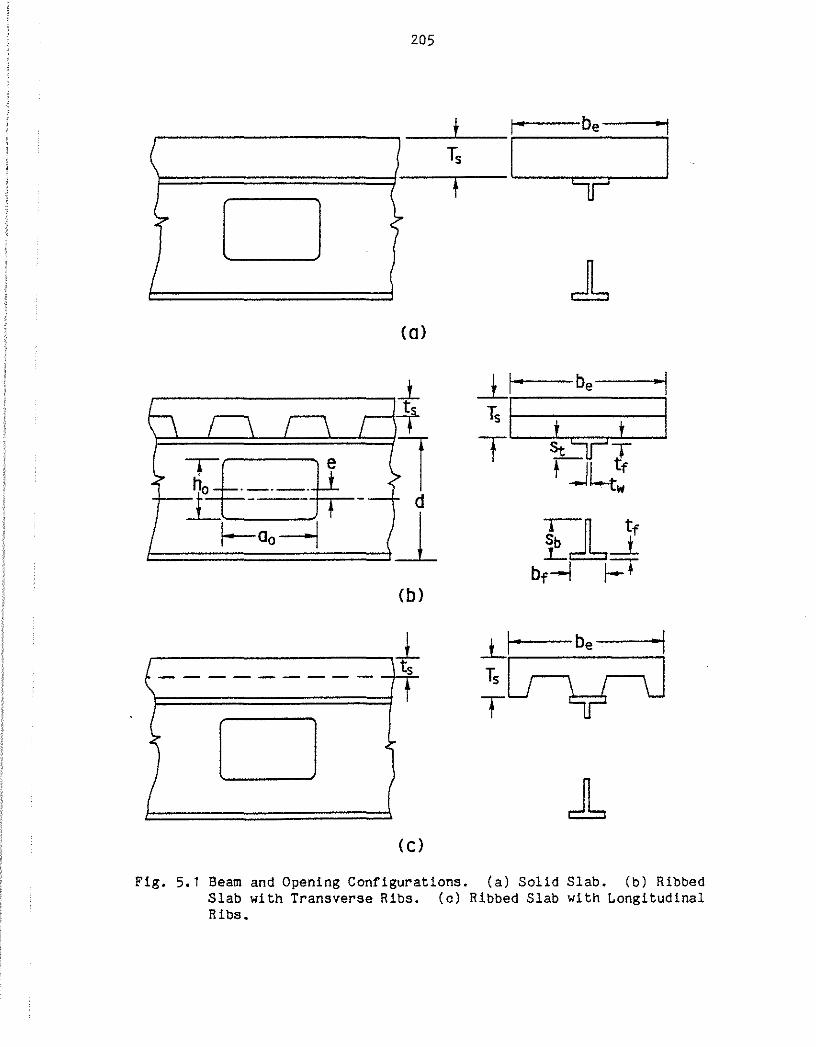
205

-----~~-r----be---i

D t

I <a>

_L be

Ts I t t T StTT

If~--#- fJL tf tw

~JL tf ~ao---J ~ _l bf~ t=T

(b)

j_ j_ be

(--------- ts

~~ t

D •" ~

l

( (C)

Fig. 5.1 Beam and Opening Configurations. (a) Solid Slab. (b) Ribbed Slab with Transverse Ribs. (c) Ribbed Slab with Longitudinal Ribs.

206

...; II

?-----.... ;:;=j~ ~

+ - ?--:----. ;:.:: "'I c ' :E:E = ~ c

:E > --

:E

~----~~----------------------------~0 c :E

0

. (J)

> t.

" u

;:.:: "' 0 .... ..., ... 0 1... "' 0 t. (1) Q) ...,

..c::: "' V) H - "' 0 00

c: .... ., - (J)

!5 0

z: N

U"\ . 00 ..... r..

r !

. tf T

T d h.-

_t

j___ tf •

n 0.85 fc' 1· "I

I.T.'_j_O I I

r e

r---. \

T St

j_

0.85fc' I • ·1

i}-"'1 0

r t-fy-i X

_i_

T

0,85fc'

}a

n I t-fy--1 _j .J

!L·-·-·-·j_ lt ~ j. - --,

1-Fy---l (O)

)

T sb

l_ 1-Fy-l

(b)

1--Fy-1 (C)

Fig, 5,3 Stress Diagrams at Maximum Moment. (a) Neutral Axis in Slab. (b) Neutral Axis in Flange. (c) Neutral Axis in Web.

}x

Mm "' 0 ....,

208

Fig. 5.4 Forces Acting at Web Opening.

Fig. 5.5 Stress Distributions for Design Method I.

0.50

0.25

209

Upper Bound to Approximation

f<xl ~ <Txyla0 l =1.</!" <1- <a,/a0 )2J1' 2

von Mlses Yield Function

P(X) ~ ( Txy /a0 l ~ 0. 69692 - 1/./3 <a, Ia, l

Best Uniform Approximation

O'x/c:To

Fig. 5.6 Best Uniform Approximation of the von Mises Yield Function for Plane Stress.

Low Moment

End

High Moment

End

Fig, 5.7 Stress Distributions for Design Methods II and III.

0 • 00 I I I I I I I I I I I I I I I I I I I I I I I Q I I I I I I I

0.00 0.25 0.50 0.75 1.00 1.25 1.50

V (test)/V n m

Fig. 5.8 Comparison of Design Method I with Test Results.

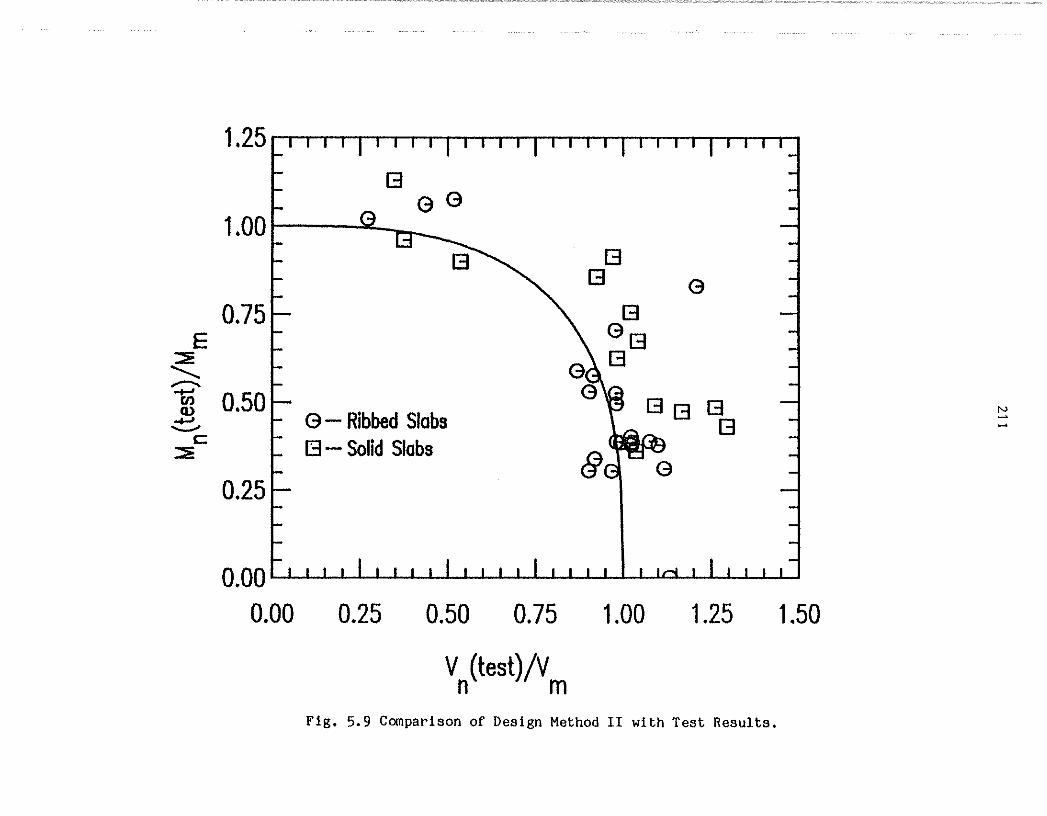
0.00 I I I I I I I I I I I I I I I I I I I I I I 10 I I I I I I I

0.00 0.25 0.50 0. 75 1.00 1.25 1.50

V (test)/V n m

Fig. 5.9 Comparison of Design Method II with Test Results.

1.25 r I

[3

G G G

1.oot 14----[3

[3 G

,.E 0.75~ .............. .

\ G~ [3

~ ~ -m o.5o . '\:; 13 1313 ~

N -~ G- R1bbed Slabs N

-::Ii. c. G- Solid Slobs t::l G G --

0.25

0 • 00 I I I I I I I I I I I I I I I I I I I I I I I I m I I I I I I

0.00 0.25 0.50 0. 75 1.00 1.25 1.50

V (test)/V n m

Fig. 5.10 Comparison of Design Method III with Test Results.

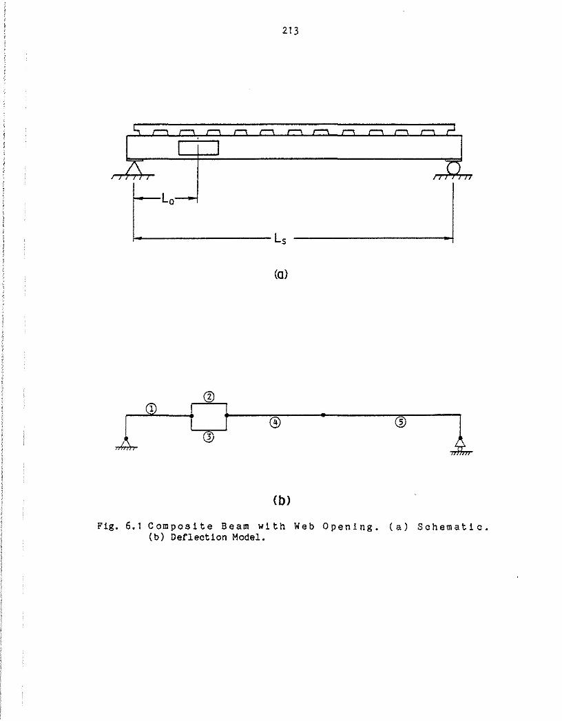
213

~----------------Ls

<a>

@

I f .__t -----,:,@,...-----· ---=®----,l

@ ~

{b)

Fig. 6.1 Composite Beam with Web Opening. (a) Schematic. (b) Deflection Model.

214

I I

Plan

I I I v'T' I 1-- 8' --~-- 8' --+- 8' 8' -l

Side

Fig. 6.2 Composite Beam in Floor System.

215

~---------------70.5"~--------------~·

z·I o o <) ~ ~ ll o " o o o ·T ~~----------~·--------------~0~--------~~--, 4"

~--------~·----~--------~~ I r----'J f 0.45"t I 0.35-- I-- 4.83"

t I" ll.O"

L t

4.83"

,.--l '-----, 1 f-6.5o--j

Fig. 6.3 Cross-Section of Composite Beam in Design Example.

a

a 0

A s

depth using

216

APPENDIX A

NOTATION

of the stress block in the a concrete stress of o.85f' c

concrete calculated

depth of the stress block in the slab at the high moment end of the opening

depth of the stress block in the slab at the low moment end of the opening

opening length

effective area for axial stress in the bottom tee

effective area for shear stress in the slab

flange area

area of reinforcing steel suggested to control crack size in the slab above the opening

stiffener area

effective area for axial stress in the top tee

web area

effective area for shear stress in a beam away from a web opening

effective area for shear stress in the top tee

effective area for shear stress in the bottom tee

total width of slab on test beam

effective width of slab

flange width

total stiffener width, including web thickness

distance from the neutral axis to the extreme compressive fiber in the slab at the high moment end of the opening

C'

cal' 1=1-4

cfi' i=1-4

c81

, i=1-4

c . 1=1-4 Wl'

D

e

e xi' 1=1-2

e yi' 1=1-2

E

E c

f

f' c

217

distance from the neutral axis to the extreme compressive fiber in the slab at the low moment end of the opening

compressive force in the steel section

constants in the bottom tee moment-axial force equations for the case when the neutral axis is in the web above the stiffener

constants in the bottom tee moment-axial force equations for the case when the neutral axis is in the flange

constants in the bottom tee moment-axial force equations for the case when the neutral axis is in the stiffener

constants in the bottom tee moment-axial force equations for the case when the neutral axis is in the web below the stiffener

coefficient of variation

steel section depth

distance from the top of the flange of the top tee to the centroid of the concrete force at the high moment end of the opening

distance from the top of the flange of the top tee to the centroid of the concrete force at the low moment end of the opening

dead load

opening eccentricity

local x eccentricities at node i for a beam element with two rigid links

local y eccentricities at node i for a beam element with two rigid links

modulus of elasticity

modulus of elasticity for concrete

normal stress in concrete

concrete strength

F u

F y

Fyf

F ys

F yw

F ywr

g

G

H s

1eff

Is

1tr

[Ke]

[Kg]

[Kg]wo

Kij

218

tensile strength of shear connector

yield strength of the steel section

yield strength of the flange in uniaxial tension

yield strength of the stiffener in uniaxial tension

yield strength of the web in uniaxial tension

the reduced longitudinal yield strength in the web due to shear

distance to the neutral axis in the top or bottom tee

distance to the neutral axis in the top tee at the high moment end of the opening

distance to the neutral axis in the top tee at the low moment end of the opening

shear modulus

opening height

rib height

stud height after welding

effective moment of inertia for the gross section

moment of inertia of a steel beam

moment of inertia of the transformed composite section

element stiffness matrix for tee

global stiffness matrix for tee

global stiffness matrix for web opening element

elements of global stiffness matrix for web opening element

length of rigid links connecting beam element to the bottom tee element

length of rigid links connecting beam elements to the top tee element

L

L s

M

M m

M n

M u

n

219

live load or length of a uniform beam element

distance from a beam support to the centerline of a web opening

beam span

primary moment at the opening centerline

secondary moment at each end of the bottom tee

secondary moment in the bottom tee at the high moment end of the opening

secondary moment in the bottom tee at the low moment end of the opening

maximum moment capacity

nominal moment capacity at a web opening

total moment at failure for test opening

primary moment at the opening centerline

secondary moment in the top tee at the high moment end of the opening

secondary moment in the top tee at the low moment end of the opening

factored moment at the opening centerline

squash load ratio

squash load ratio at crossover of the neutral axis from the web to the flange the high moment end of the bottom tee

squash load ratio at crossover of the neutral axis from the stiffener to the web below the stiffener at the high moment end of the bottom tee

squash load ratio at crossover of the neutral axis from the web above the stiffener to the stiffener at the high moment end·of the bottom tee

squash load ratio at crossover of the neutral axis from the flange to the web at the low moment end of the bottom tee

N

N 0

N r

p

Psl

pt

pth

ptl

Pwb

Pwt pf

xh

220

number of studs between the high moment end of the opening and the support

number of stud shear connectors above the web opening

number of studs per rib

axial force in tee

bottom tee axial force

bottom tee axial force at low moment end of opening

bottom tee axial force at high moment end of opening

crushing capacity of slab

concrete force at high moment end of web opening

concrete force at low moment end of web opening

steel force at high moment end of web opening

maximum capacity of top tee steel

steel force at low moment end of opening

top tee axial force

top tee axial force at high moment end of opening

top tee axial force at low moment end of opening

normal force in the bottom tee web

normal force in the top tee web

normal force in the steel tee at crossover of the neutral axis from the web to the flange at high moment end of opening

normal force in steel tee at crossover of the neutral axis from the web to the flange at low moment end of opening

normal force in steel tee at crossover of the neutral axis from the web below the stiffener to the stiffener at low moment end of opening

q

q'

Qn

r

R

sb

st

t e

tf

t s

t w

T'

T s

ugi' i=1-2

u~i' i=1-2

{U } g

{U~}

vgi' i=1-2

v~i' 1=1-2

v

vb

Vb(max)

221

normal force in steel tee at crossover of the neutral axis from the stiffener to the web above the stiffener at low moment end of opening

percentage of maximum top tee shear capacity applied to top tee

parameter for distribution of shear between top and bottom tees

nominal strength of one stud shear connector embedded in a solid slab

coefficient of correlation

reduction factor for studs in ribbed slabs

web stub depth for bottom tee

web stub depth for top tee

effective slab thickness for shear stress

flange thickness

minimum slab thickness

web thickness

yield capacity of net steel section at web opening

maximum slab thickness

global degree of freedom in the x direction at node i

local degree of freedom in the x direction at node i

global degrees of freedom for beam element

local degrees of freedom for beam element

global degree of freedom in the y direction at node i

local degree of freedom in the y direction at node i

shear force acting at opening centerline

shear assigned to the bottom tee

maximum shear capacity of bottom tee

V' h

v m

v n

vpb

vpt

Vt(sh)

Vt(max)

vtc

vtm

V (test) n

w

w r

X

X g

z

CL, 8, Y

222

smaller of the tensile yield capacity of the gross steel section or the crushing strength of the concrete slab

sum of shear stud capacities between the point of maximum moment and the nearest point of zero moment

maximum shear capacity at web opening

nominal shear capacity at web opening

plastic shear capacity of the bottom tee web

plastic shear capacity of the top tee web

"pure shear" capacity for the top tee

"mechanism" shear capacity of top tee

shear due to secondary moment from the concrete

top tee shear strength, smaller of Vt(max) and Vt(sh)

total shear at failure for web opening test

uniform load ~pplied to beam

average rib width

neutral axis location in the top tee

global coordinate x axis

local coordinate x axis for bottom tee

local coordinate x axis for top tee

distance from bottom of top tee to centroid of concrete force at high moment end of opening

distance from bottom of top tee to centroid of concrete force at low moment end of opening

distance from bottom of top tee to centroid of stiffener

distance between the axial forces in the top and bottom tees

parameters for maximum shear capacity calculation

ab

ab,

at,

0

[~

0 0

0 m

~b

~ s

8 gi'

8ii'

A

~. v

cr 0

cr X

t

tb

't

t xy

~b

~v

nb

nt

i=l-2

1=1-2

223

parameter for bottom tee maximum shear capacity calculation

element stiffness matrix parameters for the bottom tee

element stiffness matrix parameter for the top tee

normalized opening deflection at failure

eccentricity transformation matrix

deflection across web opening at failure

deflection at point of maximum moment at failure

calculated deflection considering bending only

calculated deflection considering shear only

global degree of freedom for rotation at node i

local degree of freedom for rotation at node i

coefficient in linear approximation to von Mises criterion

factors for maximum shear capacity of top tee

yield stress obtained from uniaxial tension test

normal stress, reduced for shear

shear stress in the slab

shear stress in the bottom tee web

shear stress in the top tee web

shear stress

flexural strength reduction factor

shear strength reduction factor

224

APPENDIX B

SUMMARY OF PREVIOUS EXPERIMENTAL WORK

A number of experimental investigations of composite beams with

rectangular web openings have been conducted (8, 9, 11, 19, 32, 34,

37, 41). Granade ( 19), Clawson and Darwin (9, 11), and Cho (8)

tested composite beams with solid, or flat-soffit slab construction.

Redwood and others at McGill University (32, 34, 46) tested com

posite beams with ribbed slab construction with the ribs oriented

transverse to the steel section. Prototype tests were conducted in

Illinois (37) and Australia (41). The test configurations used in

previous investigations are summarized in Tables B.1 - B.3. The

test results for the previous investigations are summarized in Table

B.4. The two prototype tests are not included in the tables. The

beam tested by Wiss, Janney, and Elstner Associates (37) failed by

longitudinal shearing of the slab near a support, and the failure

was not related to the web opening. The test conducted by Thompson

and Ainsworth (41) was not continued to failure.

225

Table B.1 Material Strengths for Previous Investigations

Yield Strengths, ksi

Top Bottom F ** f' u c Test* Flange Flange Web Stiffener ksi psi

01 43.8 43.8 47.9 N.A. 3970 02 43.8 43.8 47.9 3990 C1 39.4 40.4 38.5 N.A. 7000 C2 39.3 39.9 42.4 4200 C3 39.3 39.9 42.4 4930 C4 46.4 44.9 52.0 4460 C5 43.9 45. 1 44.2 4680 C6 42.9 43.5 49.8 4020 CH03 44. 1 43. 4 50.8 60.3 3270 CH04 54.0 50.7 64.6 60.3 3040 CH05 54.0 50.7 64.6 60.3 3270 CH06 44.1 43.4 50.8 50.8 60.3 3270 CH07 54.0 50.7 64.6 50.8 60.3 3170 RO 50.6 50.6 56.1 N. A. 3830 R1 40. 1 40. 1 45.1 --- 3190 R2 43.8 43.8 47.3 2830 R3 42.2 42.2 47.2 4290 R4 43.7 43.7 48. 1 3960 R5 40. 1 40. 1 45. 1 3190 R6 43.7 43.7 47.2 2610 R7 43.7 43.7 47.2 2610 R8 44. 1 44. 1 44.0 2480

* G- Granade (19) C - Clawson and Darwin (9, 11 ) CHO - Cho (8) R - McGill Tests (32, 34)

** Stud tensile strength N.A. indicates data not available

226

Table 8.2 Section and Opening Dimensions for Previous Investigations, in.

t bf(Top} tf(Top} tw Test d st sb G1 8.00 6.5ii 0.463 o. 285 1.630 1:63'0 G2 8.00 6.54 0.463 0.285 1 .630 1.630 C1 14.00 6.75 0.453 0.287 3.003 3.003 C2 17.88 7.50 o. 475 0.356 3.475 3. 710 C3 7.50 0. 475 0.356 3.605 3.650 C4 7.50 o. 485 0.343 3.485 3.555 C5 18.13 6.00 0.623 0.380 3.683 3.745 C6 14.00 6.69 0. 475 0.296 2.855 2.803 CH03 7.87 5.91 0.354 0.236 1.500 1. 500 CH04 11.81 5.91 0.354 0.256 2.360 2.400 CH05 11 • 81 5.91 0.354 0.256 2.400 2.320 CH06 7.87 5.91 0.354 0.236 1.540 1. 500 CH07 11 .81 5.91 0.354 0.256 2. 360 2.360 RO 9.98 4.02 0.256 0.228 2.039 2.039 R1 14.01 6.87 0.448 0. 293 2.810 2.810 R2 14.05 6.74 o. 441 0.309 2.830 2.830 R3 14.03 6.74 0.444 o. 313 2.820 2.820 R4 14.04 6.86 o. 436 0.313 2.835 2.835 R5 14.01 6.87 0.448 o. 293 1. 410 4.210 R6 14.05 6.75 0.437 0.305 2.835 2.835 R7 14.05 6.75 0.437 0.305 2.835 2.835 R8 13.98 6.69 0.450 o. 292 2.795 2. 795

Testt bf(Bot} tf(Bot} boone b * t T Opening Size e s s

G1 6.54 0.463 24.0 24.0 3.6 3.6 4.80 X 7.20 G2 6.54 0.463 24.0 24.0 3.6 3.6 4.80 X 7.20 C1 6.75 0.453 48.0 48.0 4.0 4.0 8.00 X 16.00 C2 7.50 0.520 48.0 48.0 4.0 4.0 10.81 X 21.63 C3 7.50 0.520 48.0 48.0 4.0 4.0 10.81 X 21.63 C4 7.50 0.495 48.0 45.0 4.0 4.0 10.81 X 21.63 C5 6.00 0.615 48.0 48.0 4.0 4.0 10.81 X 21.63 C6 6.69 0.423 48.0 45.0 4.0 4.0 8.00 X 16.00 CH03 5.91 0.354 21.6 21.6 5.3 5.3 4. 72 X 7. 28 CH04 5.91 0.354 23.8 23.8 5.4 5.4 7.05 X 10.63 CH05 5.91 0.354 23.8 23.8 5.3 5.3 7.09 X 10.63 CH06+ 5.91 0.354 23.8 23.8 5.3 5.3 4.61 X 7.13 CH07+ 5.91 0.354 23.8 23.8 5.3 5.3 7.09 X 14.37 RO 4.02 0.256 39.4 39.4 2.6 5.6 5.91 X 11.81 R1 6.87 o. 448 47.2 39.4 2.6 5.6 8.39 X 16.77 R2** 6.74 0.441 47.2 47.2 2.6 5.6 8.39 X 16.77 R3** 6.74 0.444 47.2 47.2 2.6 5.6 8,39 X 16.75 R4** 6.86 0.436 47.2 47.2 2.6 5.6 8,39 X 16.75 R5 6.87 0. 448 47.2 39.4 2.6 5.6 8.39 X 16.77 R6 6.75 0. 437 39.4 39.4 2.6 5.6 8.39 X 16.75 R7 6.75 0.437 39.4 39.4 2.6 5.6 8. 39 X 16.75 RS 6.69 0.450 39.4 39.4 2.6 5.6 8. 39 X 16.75

t G ~Granade (19}, C- Clawson and Darwin (9, 11 ) CHO- Cho (8), R- McGill Tests (32, 34)

* b • effective slab width (as per Reference 2) e

+ stiffeners on top and bottom tees: t5

= 0.236, b = 4.170, y = 0.374 s s

** cover plates of unknown thickness and width were welded to the bottom flange away from the opening.

227

Table 8.3 Stud and Rib Properties for Previous Investigations.

Stud + h t tt * ** Test Diameter H w N N s r r 0

in. in. in. in.

G1 5/8 2.5 2 10 G2 2 16 C1 3/4 3.0 _:,:._ 4 14 C2 2 16 C3 2 16 C4 4 10 C5 4 16 C6 4 10 CH03 1/2 3.94 4 12 CH04 4 18 CH05 4 20 CH06 4 12 CH07 4 20 RO 3/4 4.84 3.0 6.0 1 * 1 4*1 R1 1*1 4*1 R2 1*2 9*2 R3 2*2 11 *2 R4 1*0 5*1 R5 1 * 1 4*1 R6 2*0 2*2 R7 2*2 4*2 R8 2*2 4*2

+ H stud height after welding s t h rib height = r

tt = average rib width w r

* N = no. of studs over opening -- For ribbed slabs = no. of ribs *

0 of studs/rib no.

** N = no. of studs between high moment end of opening and support --For ribbed slabs = no. of ribs * no. of studs/rib

228

Table B.4 Test Results for Previous Investigations.

Reported Maximum Load

Applied Load Total Load at Opening * M M t . M v Test V at Opening Vd a opemng

(ft) (in.-kips) (kips)

G1 2.00 3.02 791 32.7 G2 4.00 6. 11 1296 26.5 C1 7.00 6.17 2886 33.4 C2 9.00 6.24 4107 36.8 C3 33.00 21.84 5468 14.0 C4 3.00 2.02 1723 47.6 C5 6.00 4.03 3511 48. 1 C6 3.00 2.60 1471 40.4 CH03 1. 48 2. 26 634 35.7 CH04 2.63 2.68 1477 46.7 CH05 10.83 10.97 2319 17.9 CH06 1.48 2. 26 721 40.6 CH07 10.83 11.95 2664 20.6 RO 3.28 4. 14 752 18. 2 R1 3. 10 2.69 978 26.0 R2 8.20 7. 20 2904 28.7 R3 19.68 17.36 3995 16.4 R4 19.68 17.49 3217 13. 1 R5 3.10 2.68 1037 27.6 R6 3. 10 2.65 788 21.2 R7 3.10 2.64 1133 30.5 R8 3.10 2.66 1075 28.9

* G - Granade (19) c - Clawson and Darwin (9, 11) CHO - Cho (8) R - McGill Tests (32, 34)

229

APPENDIX C

DETERMINATION OF NEUTRAL AXES LOCATIONS IN THE BOTTOM TEE

In the bottom tee, the neutral axis may be located within one

of two regions at the low moment end and within one of four regions

at the high moment end. The following procedure is used to establish

the neutral axis location at each end of the opening.

The moment-axial force equations for the bottom tee are given

below. The neutral axis at the low moment end of the opening is

initially assumed to be in the flange. The four possible neutral

axis locations at the high moment end of the opening are then checked

for a valid solution. If no solution is obtained, the neutral axis

at the low moment end of the oper.ing is assumed to be in the web.

The four possible locations at the high moment end are then checked

for a valid solution.

C.1 NEUTRAL AXIS IN THE FLANGE AT THE LOW MOMENT END

When the neutral axis is above the stiffener at the high moment

end of the opening, moment equiliprium requires that

2 2 2 = (Cf1cf3 + ca1ca3ln

+ 2(Cf1cf2cf3- ca1ca2ca3ln

+ c~2cf3+ c~2ca3 + cf4 + ca4 (c. 1)

230

in which cf 1' cf2 , cf3

, and Cf4 are given by Eq. (4.11a)-(4.11e) and

Ca 1' ca2 ' ca3 ' and ca4 are given by Eq. (4.19a)-(4.19e).

The crossover shear at the high moment end, Vxh' is obtained by

substituting n~h (Eq. (4.23)) for n in Eq. (C.1). The crossover

shear at the low moment end, Vxl' is obtained by substituting n~1 (Eq. (4.17)) for n in Eq. (C.1). If vb .S. vxh and vb .S. vxl' Eq. (C.1)

is valid for Vb and is solved for n.

When the neutral axis is in the stiffener at the high moment

end, moment equilibrium requires that

= cci1cf3+ c;1cs3)n2

+ 2(Cf1cf2cf3 - cs1cs2cs3)n

+ ci2cf3 + c!2cs3 + Cf4+ cs4 (c. 2)

in which cs 1, cs 2 ' cs3

, and cs 4 are given by Eq. (4.21a)-(4.21e).

Vxh is obtained by substituting n~h (Eq. (4.25)) for n in Eq.

(C.2), while Vxl is obtained by substituting n~1 (Eq. (4.17)) for n

in Eq. (C.2). If vb .S. Vxh and vb .S. vxl' Eq. (C.2) is valid for vb

and is solved for n.

When the neutral axis is in the web at the high moment end,

moment equilibrium requires that

231

?. 2 2 = ccf,cf3+ cw,cw3)n

+ 2(Cf1cf2cf3 - cw,cw2cw3ln

+ c~2cf3 + c!2cw3 + Cf4+ cw4 (C.3)

in which Cwl' cw2' cw3

, and cw4 are given by Eq. (4.15a)-(4.15e).


(C.3), while Vxl is obtained by substituting n~1 (Eq. ( 4.17)) for n

in Eq. (C.3). If vb i vxh and vb i vxl' Eq. (C.3) is valid for vb

and is solved for n.

When the neutral axis is in the flange at the high moment end,


f Vxl is obtained by substituting nxl for n in Eq. (C.4). If Vb i Vxl'

Eq. (C.4) is valid for Vb and is solved for n.

C.2 NEUTRAL AXIS IN THE WEB AT THE LOW MOMENT END

When the neutral axis is above the stiffener at the high moment

end of the opening, moment equilibrium requires that

232

(C.5)


(C.5). If Vb ~ Vxh , Eq. (C.5) is valid for Vb and is solved for n.

When the neutral axis is in the stiffener at the high moment

end, moment equilibrium requires that

2 2 2 = (Cw1cw3+ cs1cs3)n

+ 2(Cw1cw2cw3 - cs1cs2cs3)n 2 2

+ cw2cw3 + cs2cs3 + cw4+ cs4 (C.6)


(C.6). If Vb ~ Vxh' Eq. (C.6) is valid for Vb and is solved for n.

When the neutral axis is in the web at the high moment end,


(C.7)

233

f Vxh is obtained by substituting nxh (Eq. (4.27)) for n in Eq.

(C.7). If Vb ~ Vxh' Eq. (C.7) is valid for Vb and is solved for n.

When the neutral axis is in the flange at the high moment end,

Vxh is obtained by substituting n~h (Eq. (4.27)) for n in Eq. (C.3).

If Vb ~ Vxh' Eq. (C.3) is valid for Vb and is solved for n.

234

APPENDIX D

MECHANISM SHEAR CAPACITIES OF TOP AND BOTTOM TEES

FOR COMPARISON WITH TEST DATA

For comparison with test data, the bottom and top tee shear

capacities are calculated using separate values for the web and

flange yield strengths, as follows:

BOTTOM TEE

in which a = 3 +

a - Ia' - 4aY 2a

F (b -2/3 yf f

sb

+ 2/3 A F t sb + 2a [F f(bf - t ) + AF t ) yw w o y w yw w

and A= 1.207.

(D. 1 )

Fyf = flange yield strength and Fyw =web yield strength for

the bottom tee.

TOP TEE

in which a. = 3 +

235

a - la 2 - 4aY

2a

+ /§"(P - p ) ch cl

(D. 2)

+ 2 /§"(P d st ch h

F yf = flange yield strength and- F yw = web yield strength for

the top tee.

E. 1 GENERAL

236

APPENDIX E

DEFLECTIONS

The introduction of a web opening in a composite beam can have

a significant affect on the beam deflection. The reduced stiffness

at the opening will cause both an increased maximum deflection and a

differential deflection across the opening. In some cases, these

increased deflections may be unacceptable. Thus, there is a need for

an analysis procedure which predicts the total and local deformations

due to web openings.

Deflection analysis procedures that consider the effects of web

openings in steel and in composite beams have been proposed ( 16, 17,

26, 27, 38) . Whi 1 e one of these procedures ( 16) has been shown to

provide reasonable agreement with data for steel beams, no com

parisons have been made with data for composite beams. Procedures do

exist for obtaining the deflection of composite sections without

openings (19, 34).

The deflection analysis procedures for steel beams with web

openings (16, 17, 26, 27, 38) require that the deflected shape of the

unperforated section be calculated. Deflections due to the web

opening are then added to those found for the unperforated section.

The Subcommittee on Beams with Web Openings of the Task

Committee on Flexural Members of the Structural Division of the ASCE

(38) has proposed an approximate procedure which models the portions

237

of the beam above and below the web opening as cantilevered tees with

the low moment end fixed. One half of the shear at the opening is

applied as a concentrated load to the free end of each tee, The

deflection of the beam from the high moment end of the opening to the

support is found by enforcing compatibility of vertical displacement

and rotation at the high moment end of the opening. The deflection

of the beam from the low moment end of the opening to the other

support is ignored. Only the bending deflection of the tees is

considered. Also, no consideration is made for slope compatibility

at the low moment end of the opening or for axial deformation of the

tees. While no comparisons with test results have been published,

the subcommittee reports that the procedure is conservative.

McCormick has proposed an approximate procedure in which points

of contraflexure are assumed to be at the opening centerline (26,

27). Bending and shear deformations of the tees are considered, but

compatibility at the opening ends is not enforced. McCormick sug

gests that no composite action should be considered at the web

opening in composite beams. No comparisons with experimental results

are made.

Dougherty considers the bending and shear deformation of the

tees and enforces compatibility of vertical displacement and slope at

ends of the opening (16, 17). Axial deformation of the tees is

neglected. Dougherty also proposes an empirical procedure for find

ing the inelastic deformation of steel beams with openings.

238

Both McCormick and Dougherty assign shear to the tees in

proportion to their relative flexural and shear stiffnesses.

Dougherty's procedures give good results when compared with ex

perimental work (16).

Granade (19) and Redwood and Wong (34) compare calculated

deflections of unperforated composite beams with measured deflections

of composite beams with web openings. Granade considers only bending

of the gross section, while Redwood and Wong consider both bending

and shear deformations. In both cases, the analyses are too stiff,

and the predicted total deflections are slightly low.

Obviously, the introduction of a web opening will have an

effect on the stiffness of a beam. A web opening will reduce the

beam stiffness by:

1) Lowering the gross moment of inertia at the opening,

2) Eliminating strain compatibility between the tees at the

opening, and

3) Reducing the amount of material available to transfer shear

at the opening.

While the first reduction will result in increased curvature at

openings subjected to bending, the second and third reductions will

result in Vierendeel (differential) deflections across openings

subjected to shear.

To correctly calculate the deflection of a beam, equilibrium,

compatibility, and material properties must be satisfied throughout

the span. A complete analysis will consider both bending and shear

239

deformation. Although classical methods incorporating all of these

requirements can be developed, it is possible to obtain equivalent

results (within the accuracy of any assumptions) using matrix

methods. The matrix approach is particularly attractive since it can

automatically enforce compatibility of displacement and rotation at

the ends of an opening.

In the following sections, the stiffness method of matrix

analysis is applied to beams with web openings. Experimental data

are used in a parametric study to determine the importance of includ-

ing shear deformation in the analysis. Recommendations for the

practical application of the procedure are made.

E.2 ANALYSIS PROCEDURE

Fig. E.1 illustrates a web opening in a composite beam. The

opening is of length a0

and depth h0

• The beam span and the opening

location are L and L , respectively. Section dimensions at the s 0

opening are as shown (Fig. E. 1b). The web adjacent to an isolated

opening is considered to be infinitely rigid. If the portions of the

beam above and below the opening, the top and bottom tees, are

modeled as uniform beam elements, a web opening element consisting of

two beam elements connected by rigid links can be developed.

A web opening element (Fig. E.2) is constructed using four

rigid links and two beam elements. The nodes of the web opening

element are connected to the ends of the top and bottom tee elements

by rigid links of length lt and lb, respectively.

240

Nodes 1 and 2 of the web opening element are located so that

the positive global coordinate x axis, x , passes through the nodes. g

The local coordinate x axes for the tee elements, xt and xb, pass

through the centroids of the respective tees. The web opening ele-

ment stiffness matrix is developed using an eccentricity

transformation (13).

A beam element with two rigid links, representing a top tee, is

shown in Fig. E.3. The local and global x axes are parallel, and

eccentricities in both x and y directions exist at each node (Fig.

E.3a). The local degrees of freedom for the beam element, {Ut}, are

given by

(E.1)

.and the global degrees of freedom for nodes 1 and 2, \U J, are given g

by

{Ug}T = [ug1' vg1' eg1' ug2' vg2' eg2}

as shown in Fig. E.3b.

(E.1a)

An eccentricity transformation matrix, [6], relates the local

element degrees of freedom and global degrees of freedom of nodes 1

and 2.

= [6]{U } g

(E.2)

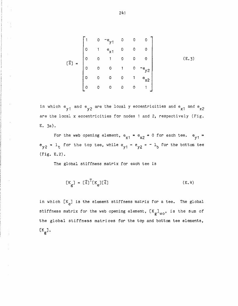
241

0 -e y1 0 0 0

0 ex1 0 0 0

0 0 0 0 0 (E.3) [6] =

0 0 0 0 -e y2

0 0 0 0 ex2

0 0 0 0 0

in which ey 1 and ey2 are the local y eccentricities and ex 1 and ex2

are the local x eccentricities for nodes 1 and 2, respectively (Fig.

E. 3a).

For the web opening element, ex1 = ex2 = 0 for each tee. ey1 =

ey 2 = lt for the top tee, while ey1 = ey2 = - lb for the bottom tee

(Fig, E.2).

The global stiffness matrix for each tee is

(E.4)

in which [Ke] is the element stiffness matrix for a tee. The global

stiffness matrix for the web opening element, [K ] , is the sum of g wo

the global stiffness matrices for the top and bottom tee elements,

242

[K ], the stiffness matrix for a uniform beam element incore

porating both shear and axial deformation, is (13)

A/8 0 0 -AlB 0 0

1 L/2 0 -1 L/2

(L 213 + n) 0 -L/2 (L2/6 - n) [K ] = ES/L (E.5) e AlB 0 0

SYM, -L/2

(L213 + n)

in which E = the modulus of elasticity, B = II(L 2/12 + n), n =

EI/(A G), A = the effective shear area, A= the gross transformed y y

area for axial deformation, L = the element length, and I = the

moment of inertia for the transformed section.

The tee elements in the web opening element are of length a • 0

Therefore, substituting for L and adding the global stiffness

matrices for the top and bottom tee elements gives [K ] . g WO

K11 K12 K13 K14 K15 K16

K22 K23 K24 K25 K26

[Kg]wo = E/a K33 K34 K35 K36 0

K44 K45 K46

SYM. K55 K56

K66

(E.6)

245

Away from the opening, the web of the steel section carries all

of the shear. Thus,

in which d

E.1b).

A = dt y w

the steel section depth and t w

(E. B)

the web thickness (Fig.

Moments of inertia for the individual tees at the opening are

calculated considering the steel tees only. The concrete is not

considered to be effective for the top tee moment of inertia. Web

openings subjected to moderate or high amounts of shear display

cracking of the concrete over the opening at relatively low loads.

Also, it is likely that only limited composite action develops over

the opening at service loads (low slip). The concrete slab will,

therefore, add only a small amount to the bending stiffness of the

top tee.

The effective area of the top tee, At, is calculated using the

area of the top tee steel plus the transformed area of the concrete

at the opening. Thus, the centroid of the top tee element is the

centroid of the transformed section of the top tee.

At the opening, the webs of the steel tees carry the shear.

Thus,

(E.9a)

246

and

in which st = the top tee stub depth and sb

depth (Fig. E.1b).

(E.9b)

the bottom tee stub

ksi.

Steel sections are modeled using E = 29,000 ksi and G = 11,150

Concrete is modeled using E = 57/fl ksi; f' in psi. c c

E.4 PARAMETRIC STUDY

E.4.1 General

In this section, the proposed deflection analysis procedures

are compared with the results of twenty-five tests. The calculated

deflections are compared with measured deflections at 30 and 60

percent of the ultimate load. The analyses are made using POLO-

FINITE (24).

To study the importance of shear deformation on beam deflec-

tion, the beam deflections are calculated either 1) considering shear

deformations throughout the span (V) or 2) ignoring shear deforma-

tions throughout the span (NV),

As a preliminary step in the study, the analysis procedure was

tested for its sensitivity to the number of elements used to model a

beam. A single beam was analyzed using 5, 9, and 11 elements, repre-

senting models with 3 gross section and 2 web opening elements; 7

gross section and 2 web opening elements; and 7 gross section and 4

web opening elements, respectively (Fig. E.4). The maximum variation

247

in deflection at the maximum moment location was 0.2%. Because the

analyses were not sensitive to the number of elements, most models

use 5 elements. The single exception is Test 6A from the current

study, which requires 6 elements.

The test beams are modeled using rigid links at the supports in

addition to the rigid links at the web opening (Fig. E.4). The links

at the supports connect the node at the bottom flange of the beam to

the centroid of the transformed section. All openings are modeled

with two eccentric beam elements (Fig. E.4a), with one element for

each tee. This combination is equivalent to the single web opening

element defined in Eq. (E.6).

The deflection data used in the parametric study include 13

tests from the current study, 6 tests by Clawson and Darwin (9, 11),

2 tests by Granade (19), and 4 tests by Redwood and Wong (34). Two

of the beams tested by Redwood and Wong had cover plates. The width

and thickness of these plates was not published; a cover plate of the

same thickness and width as the beam flange is assumed. The data for

4 tests conducted at McGill and for Cho's tests were not published in

a useable form. Two openings in the current study (Beams 4A and 4B)

and the fourth opening tested by Redwood and Wong had no studs over

the opening and are excluded from the parametric study.

The comparisons that follow should be prefaced by a comment on

a built-in bias of the test results. The tests were designed

primarily to obtain data on the strength at web openings; the beams

were relatively short and opening locations in high shear regions

248

predominated. For this reason, the relative importance of shear

deformation and deflection through the opening will be greater than

for longer beams in which flexural deformation plays a greater role.

E.4.2 Comparison with Test Data

The following comparisons are based on deflections under ap

plied load (i.e., dead load deflections are not considered).

Calculated and measured deflections at the point of maximum moment

and through the opening are compared for the two models (V and NV) in

Fig. E.5-E.8. The measured and calculated deflections for each test

are also presented in Tables E.1 and E.2, along with the ratios of

calculated to measured deflection for the models. The tables include

the mean ratios of the calculated to measured deflection, along with

the standard deviation and the coefficient of variation for the two

models. The deflections across the opening are compared with the

total deflections, both for the test and calculated results, in Table

E.3.

Overall, both models provide reasonable agreement with test

results for total deflections at the point of maximum moment. The

models provide somewhat poorer agreement with test results for

deflections through the opening. In most cases, model V provides

better agreement with test results for total deflections, while model

NV provides better agreement with test results for deflections across

the opening. The ratios of calculated to measured deflection

decrease as the load is increased from 30 to 60 percent of the ap-

plied load at ultimate, reflecting the relatively early onset of

yield at the openings (Chapter 3).

At both 30 and 60 percent of the ultimate load, on the average

model V provides good agreement with test results for total deflec-

tions, while model NV is too stiff (Fig. E.5 and E.6 and Tables E.1

and E.2). However, some individual tests deviate appreciably from

the calculated deflections. At 30 percent of ultimate load, the

average ratios of calculated to measured deflection for models V and

NV are 1.155 (coefficient of variation, C = 26.1 percent) and 0.996 v

(C = 26.6 percent), respectively. At 60 percent of ultimate load, v

the average ratios of calculated to measured deflection are 1.025 (C v

= 20.8 percent) and 0.882 (C = 2>.3 percent), respectively. v

For total deflections, model V is stiff when compared with test

results for openings with high shear-span to depth ratios, M/Vd. At

30 percent of ultimate load, the ratios of calculated to measured

deflection are 0.951, 0.741, and 0.991, for Tests 3 (M/Vd = 26.30),

R3 (M/Vd = 16.83), and C3 (M/Vd = 22.14), respectively. These repre-

sent the lowest ratios of calculated to measured deflection for each

of the respective test series. However, model V is very flexible

when compared with test results for openings with relatively stiff

slabs and low M/Vd ratios. Tests 8A, 88, 9A, and 9B had relatively

stiff slabs as compared to the steel tees at the opening. The ratios

of calculated to measured deflection for the four tests are 1.652,

1.713, 2.069, and 1.624.

250

Both models exhibit large scatter when compared with the

deflection across the opening (Fig. E. 7 and E. 8). At 30 percent of

ultimate load, both models are too flexible when compared with most

test data (Table E.1). At 60 percent of ultimate load, the models

are better, but on the average are still flexible when compared with

test results (Table E.2). Six of the tests were considerably stiffer

than the models (88, 9A, 98, RO, C1, and C4). Tests 8A-98 had rela

tively stiff slabs as compared to the steel tees at the opening.

Tests RO, C1, and C4 had very small measured deflections across the

openings (less than 0.062 in. at 60 percent of ultimate load), al

though they had relatively low M/Vd ratios. Low deflections tend to

amplify the effects of other factors, such as measurement errors and

seating errors in the beam. These six tests tend to skew the data,

resulting in mean ratios of calculated to measured relative deflec

tion that indicate a flexible model.

These comparisons with test results suggest that in some cases

the models may be improved by the addition of partial composite

action at the opening. However, sizeable improvement will likely

require the consideration of non-linear materi·al response.

The relative importance of the deflection across the opening to

the total deflection is considered in Table E.3. Ratios of the

deflection across the opening to the total deflection are summarized

for the measured deflections at 30 and 60 percent of ultimate load

and for the calculated deflections. In most cases, the ratios for

measured deflection are relatively constant as the load increases

251

from 30 to 60 percent of ultimate, while the ratios obtained for the

two models compare well with each other. Also, in most cases, the

ratios for the calculated deflections agree with the ratios for the

measured deflections. Noteable exceptions are Tests 8B, 9B, and C4,

three tests for which the models greatly overestimate the deflection

across the opening.

As would be expected, the relative importance of the deflection

across the opening tends to decrease with increasing M/Vd ratio.

Tests 3, R3, and C3 have the highest M/Vd ratios for their respective

test groups and have the lowest ratios of deflection across the

opening to total deflection.

E.4.3 Case Study

The deflection analysis procedures generally provide good

agreement with test results for total beam deflection. However, the

test results were obtained from beams which were not typical of beams

used in buildings. Most of the test beams had relatively short spans

and all of the test beams were loaded using point loads.

A limited study of composite beams with uniform loads is con

ducted to determine the effects of web openings on uniformly loaded

beams. W21 x 44 steel beams with a 6 in. composite ribbed deck (3

in. ribs) are modeled. The beams are spaced at 8 ft and are loaded

with a uniform load of 1.52 kips/ft (equivalent to a live load of

0.128 kips/ft2 and a dead load of 0.062 kips/ft 2). Two spans, 40 ft

and 20 ft, are considered. The beams are modeled assuming E = 29,000

252

ksi, G= 11,150 ksi, AY= 7.32 in~, andieff= 2936 in? A 12-3/8 x

24-3/4 in. opening is placed in the beam. The distance of the open-

ing centerline from the support, L0

, is varied from 4 to 20 ft for

the beams with span length Ls = 40 ft and is varied from 4 to 10 ft

for the beams with L =20ft (Fig. E.1a). Shear deflections through s

the span are considered and ignored in separate analyses. Similar

beams with no openings are also modeled.

The results of the analyses are summarized in Table E.4. As

the table indicates, the effect of the opening on the centerline

deflection is relatively small for the beams with 40 ft spans, but is

somewhat higher for the beams with 20 ft spans. The greater relative

effect of the openings on the shorter beams is due to the fact that

the opening represents a greater portion of the span.

For the beams with 40 ft spans, the ratio of the centerline

deflection with an opening to the centerline deflection without an

opening decreases from 1. 054 to 1. 044 (model V) as the opening is

moved from 4 ft from the support to midspan. In this case, the

effect of shear deformation through the span is nearly independent of

opening location. The ratio of the centerline deflection considering

shear to the centerline deflection ignoring shear varies from 1.048

to 1.043 as the opening moves from 4ft from the support to midspan,

while the calculated ratio for the beam without an opening is 1.046.

For the beams with 20 ft spans, the ratio of the centerline

deflection with an opening to the centerline deflection without an

opening decreases from 1.286 to 1.058 (model V) as the opening is

253

moved from 4 ft from the support to midspan. The ratio of centerline

deflection considering shear to the centerline deflection ignoring

shear drops from 1.179 to 1.164 as the opening moves from 4ft from

the support to midspan, while the ratio for the beam without an

opening is 1.203.

The maximum deflection for the beams with a 40ft span is 1.136

in. and occurs when the opening is 4 ft from the support. This

deflection is equivalent to L /423 and is well within the limit set s

by the Uniform Building Code (43) for live load plus dead load

deflection (L /240). Since the beams are over-designed for the 20ft s

span, the deflections are so small under the given loads as to be of

no consequence.

Using classical beam theory for a uniformly loaded beam, the

ratio of maximum deflection considering bending and shear to the

maximum deflection considering only bending, (6b + 6s)/6b, can be

shown to be

= 1 + 48Eieff

5A G L2 y s

(E.10)

This ratio is 1.044 and 1.174 for the beams with 40 and 20 ft spans,

respectively. The ratios compare well with the results obtained from

the matrix analysis, suggesting a practical alternative to model V;

to include the effect of shear deflection, the total deflection of

254

beams with web openings can be obtained by multiplying the deflec

tions obtained with model NV by Eq. (E.10). The ratios also show

that the error caused by ignoring shear deflection is about the same,

with or without a web opening.

One more comparison is in order. That is a comparison of an

accurate estimate of true total deflection (model V) with the deflec

tion obtained by ignoring both the opening and the effects of shear

deflection. The latter case is, of course, the standard used in

building design.

In the case of the 40 ft span, the ratio of the V model deflec

tion with an opening to the NV model deflection without an opening

ranges between 1.09 and 1.10. For the 20ft span, the ratio ranges

from 1.28 to 1.55. For long spans, the contribution of the two

effects still represents only a small portion of the total

deflection. However, for shorter spans or long spans with multiple

openings, these effects can be significant and should be included in

the analysis.

This comparison suggests some useful future research: The

development of a design aid with factors, based on opening size and

location, that would be applied to the bending deflection of a beam

without an opening to obtain an accurate estimate of total deflection

with an opening.

255

E.5 RECOMMENDATIONS

Model V provides reasonable results when compared with the test

results for total deflection, while model NV is about 12 percent too

stiff when compared to total deflections at 60 percent of ultimate.

Neither model provides a good correlation with test results for the

deflection across the opening. However, both models are, on the

average, more flexible through the opening than the test specimens

and are therefore conservative for design applications.

The case study indicates that a web opening has an increasing

effect on deflection as both the shear at the opening and the rela

tive size of the opening are increased. The case study also

indicates that the deflections obtained with model NV can be modified

to include shear effects by multiplying by Eq. (E.10).

Based on this limited study, a number of practical alternatives

for estimating total deflection exist. The most accurate estimates

can be obtained with the model V. Similar results, with little loss

in accuracy, can be obtained by multiplying the. deflections obtained

with model NV by Eq. (E.10). Ignoring both shear deflections and the

opening can lead to significant errors in estimates of total

deflections.

Table E. 1 Measured and calculated deflections at 30 percent of ultimate load.

Deflection at Point of Maximum Moment Deflection across Oeenins

Calculated- Calculated-Deflection, in. Measured Deflection, in. Measured

• Calculated Ratio Calculated Ratio Test M/Vd Measured v NV v NV Measured v NV v NV -1- :G)~ 0,116 O.l28 0. 110 1.l06 o-:91!5 0.065 0.071 o:06li 1.098 0.987 2 3.78 0.137 0.137 o. 117 0.997 0.853 0.060 0.066 0.058 1. 103 0.966 3 26.30 0.211 0.201 o. 175 0.951 0.829 0.052 0.027 0.025 0.517 0.1!77 5A 3.78 0. 111 0.132 o. 116 1. 193 1. 0~11 0.052 0.059 0.052 1.134 0.995 58 3.78 o. 128 0.132 o. 115 1. 034 0.897 0.081 0.084 0.073 1. 034 0.907 6A 0.00 0.048 0.01!9 0.035 1.013 0.733 0.047 0.052 0.01!6 1 • 1 01 0.968 68 2.04 0.108 0.123 0.104 1. 140 0.967 0.066 0.083 0.073 1. 251! 1. 106 7A 2.01! 0.11!7 o. 171! 0. 1511 1. 182 1. 01!9 0.061 0.089 o. 081 1.458 1. 323 78 3.78 0. 199 o. 211 o. 189 1.060 0. 951 0.061 0,081! 0.076 1.371! 1. 238 N

\J1 8A 3.89 0.062 0.102 0.087 1. 652 1.402 0.033 0.046 0.038 1. 379 1.160 "' 8B 2.90 0. 06!1 0.110 0.091 1.713 1. 519 0.028 0. 101 0.094 3.621 3.362 9A 2.04 0.057 0. 118 o. 101 2.069 1. 779 0.055 0. 115 o. 106 2.088 1. 918 98 1. 75 o. 100 0.162 o. 141 1.624 1 • 1!07 0.01!6 0. 159 0.11!6 3.1!63 3.171 RO 3.94 0.153 0.144 0.124 0.940 0.811 0.031 0.053 0.01!8 1 .702 1.535 R1 2.66 0.100 0.081 0.066 0.807 0.662 0.038 0.050 0.01!3 1. 307 1. 143 R2 7.00 0.233 o. 173 o. 157 0.741 0.675 0.047 0.039 0.034 0.836 0.726 R3 16.83 0.272 0.279 0.252 1.027 0.928 0.017 0.024 0.020 1. 400 1.156 C1 6.00 0.329 0.344 0.319 1. 047 0.968 0.051 0.070 0.062 1. 379 1. 217 C2 6.04 o. 274 0. 276 0.252 1.008 0.921 0.060 0.068 0.061 1. 138 1.017 C3 22.15 0.285 0.282 0.256 0.991 0.897 0.028 0.036 0.034 1. 293 1. 219 C4 2. 01 0.091 0.112 0.092 1. 228 1. 01 2 0.023 0.081 0.070 3.508 3.058 C5 3.97 0.186 0.209 0. 186 1. 123 1. 001 0.059 0.079 0.069 1. 333 1. 175 C6 2.57 0.124 o. 148 0.124 1. 193 1.001 0.048 0.072 0.062 1.509 1. 293 Gl 3.00 o. 108 0.107 0.086 0.987 0.795 Mean 1. 566 1. 292 G2 6.00 0.128 0.136 0. 110 1.059 0.857 Std. Dev. 0.833 0.763 Mean 1. 155 0.996 Coeff. of Variation 53.2% 59.1% Std. Dev. 0.302 0.265 Coeff. of Variation 26. 1% 26.6%

• Based on applied load

Table E. 2 Measured and calculated deflections at 60 percent of ultimate load.

Deflection at Point of Maximum Moment Deflection across OEenin~

Calculated- Calculated Deflection, in. Measured Deflection, in. Measured

• Calculated Ratio Calculated Ratio Test M!Vd Measured v NV v NV Measured v NV v NV -1-2:04 0.256 0.257 o:-:?19 1.002 0:857 0.170 0.142 0.127 0.834 0.748 2 3. 78 o. 305 0. 272 0.233 0.892 o. 763 o. 161 o. 132 0.116 0.822 0.720 3 26.30 0.447 0.400 0.350 0.896 0.782 0.088 0.053 0.049 0.600 0.553 5A 3.78 0.244 0.264 0.231 1. 081 0.945 0. 127 0. 118 0.103 0.929 0.815 58 3.78 0.303 0.264 0.229 0.871 0.755 0.214 o. 167 0.146 o. 778 0.682 6A o.oo o. 107 0.096 0.070 0.899 0.657 o. 149 0. 103 0.090 0.694 0.895 68 2.04 0.246 0.245 0.208 0.997 0.845 0.162 0.166 0.145 1.022 0.453 7A 2.04 0.321 0.348 0.308 1.083 0.960 0.150 o. 177 o. 160 1. 179 1. 069 7B 3. 78 0.409 0.421 0.378 1.029 0.923 0.130 0.167 0.150 1. 281 1. 154 N 8A 3.89 0.159 0. 192 0. 160 1. 210 1. 008 0.090 0.087 0.077 0.966 0.851 'Vl

" 88 2.90 0. 146 0. 218 o. 193 1.495 1. 325 0.102 0.202 o. 187 1. 978 1.836 9A 2.04 0.152 0.236 0.203 1. 552 1. 334 0. 174 0.230 0.210 1. 320 1. 207 .9B 1. 75 0.223 0.325 0.280 1.457 1. 257 0.130 o. 319 0.292 2.451 2. 244 RO 3.94 0.272 0.287 0.248 1.053 0.913 0.062 0.104 0.093 1.685 1.502 R1 2.66 0.230 0.161 0.131 0.702 0.571 0.115 0.098 0.085 0.855 0.738 R2 7.00 0.453 0.344 0.313 0.760 0.692 0.096 0.078 0.068 0.808 0. 711 R3 16.83 0.585 0.558 0.504 0.953 0.861 0.033 0.048 0.039 1. 442 1 • 191 C1 6.00 0.836 0.689 0.637 0.824 0.762 0.034 0. 1110 0.124 4.108 3.651 C2 6.04 0.643 0.552 0.504 0.859 o. 7811 0.154 o. 137 0.122 0.887 0.793 C3 22. 15 0.679 0.5611 0.511 0.830 o. 753 0.073 0.072 0.067 0.992 0.921 C4 2.01 0.216 0.223 0.183 1. 034 0.8118 0.058 o. 161 o. 141 2. 782 2.426 C5 3.97 0.403 0. 417 0.371 1.034 0.922 0.139 0. 157 0.139 1 • 131 0.997 C6 2.57 0.277 0. 295 o. 248 1.064 0.896 0.116 0.145 0.124 1. 249 1.070 G1 3.00 0.216 0.213 o. 171 0.987 0.790 Mean 1.339 1.189 G2 6.00 o. 255 0.270 0.218 1. 059 0.856 Std. Dev. 0.816 o. 729 Mean 1.025 0.882 Coeff. of Variation 60.9% 61.3% Std. Dev. 0.213 0.188 Coeff. of Variation 20.8% 21.3%

• Based on applied load

258

Table E.3 Ratios of Deflection across the Opening to to Deflection at the Point of Maximum Moment.

Ratios for Ratios for Measured Calculated

* Deflection Deflection

Test M/Vd 30% 60% v NV 1 2.04 0.560 0.664 0.555 0.582 2 3.78 0.438 0.528 0.482 0.496 3 26.30 0.246 0. 197 o. 134 0.143 5A 3.78 0.468 0.520 0.447 0.448 58 3.78 0.633 0.706 0.636 0.635 6A 0.00 0.979 1 • 393 1 • 061 1 • 314 68 2.04 0. 611 0.659 0.675 0.701 7A 2.04 0.415 0.467 0. 511 0.526 78 3.78 0.307 0.318 0.398 0.402 8A 3.89 0.532 0.566 0.451 0.437 88 2.90 0.438 0.699 0.918 0.969 9A 2.04 0.965 1 • 1 45 0.975 1. 050 98 1. 75 0.460 0.583 0.981 1. 035 RO 3.94 0.203 0.228 0.368 0.387 R1 2.66 0.380 0.500 0.617 0.652 R2 7.00 0.202 0.212 0.225 0.217 R3 1 6. 83 0.063 0.056 0.086 0.079 C1 6.00 0.155 0. 041 0.203 0. 194 C2 6.04 0.219 0.240 0.246 0.242 C3 22. 1 5 0.098 0. 1 08 0.128 o. 133 C4 2.01 0.253 0.269 0.723 0. 761 C5 3.97 0.317 0.345 0.378 0.371 c6 2.57 0.387 0.419 0.486 0.500

* Based on applied load

259

TableE.4 Effect of a 12-3/8 x 24~3/4 in. Web Opening on the Deflection of a W21 x 44 Composite Beam.

40 ft Span Centerline

Opening- Across Opening Opening Deflection V-NV No Opening Deflection V NV

Location Model in. Ratio Ratio in. Ratio 4 v 1. 136 1. 048 1. 054 0.271 1.063 4 NV 1. 084 1. 051 0.255

6.5 v 1. 133 1. 047 1. 051 0.240 1. 062 6.5 NV 1. 082 1. 049 0. 226

9 v 1 • 131 1. 045 1. 049 0.204 1. 068 9 NV 1. 082 1. 049 0. 191

14 v 1. 132 1. 044 1. 050 o. 117 1. 054 1 4 NV 1. 084 1. 051 0. 111 20 v 1. 125 1. 043 1. 044 o.ooo 20 NV 1. 079 1. 047 0.000

No Opening v 1. 078 1. 046 No Opening NV 1. 031

20 ft SEan Centerline

Opening- Across OEenin~ Opening Deflection V-NV No Opening Deflection V-NV

Location Model in. Ratio Ratio in. Ratio 4 v 0.099 1. 179 1. 286 0.056 1.120 4 NV 0.084 1. 313 0.050

10 v 0.082 1. 164 1. 058 o.ooo 10 NV 0.070 1. 094 o.ooo

No Opening v 0.077 1. 203 No Opening NV 0.064

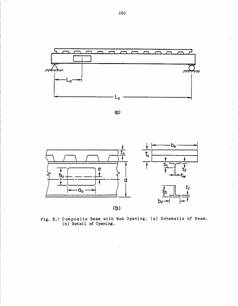
260

(O)

(b)

_j_f---be--...j

Ts 11---t --.--1

T StTT fJLt~

Fig. E.1 Composite Beam with Web Opening. (a) Schematic of Beam. (b) Detail of Opening.

Yg ~ Yt ~ Yb

Oo

,;-Top Beam Element

J ..

tt

· Rlgld Links " +-~-----.. 1 2 ... £

L ~

Bottom Beam Element

Fig. E.2 Web Opening Element Geometry and Axes Orientations.

Xt

-Xg

Xb

N <1' -

262

Beam Element

2 1 ·~~~--------------------------------•~--~--~xg

Yg

exl ~2

(O)

Beam Element

1 Ugl

(b)

2 -xg Ug2

Fig. E.3 Beam Element with Two Rigid Links. (a) Global and Local Axes. (b) Global and Local Degrees of Freedom.

® P/

2

1 r" @ ® ®

.i~ ® ;~ . .. . .

Q) ®

1\ ,_ '""

Q)_@

,/:>,,

® ® (j) '-.../ '-'

® P/

2

1 r ®

®® ®I • ® P/21 !P/2

® . @ @

®-0

Fig, E.~ Deflection Analysis Model for Beam with Web Opening. (a) 5 Element Model. (b) 9 Element Model. (c) 11 Element Model.

~ If IIIII

jt .. - I.F/1

<a>

(b)

(C)

N o-w

a)

b)

.5 c:

J5 g

264

I

I I

r;,+l x'VI I

I

I

/ /,_o+

//

I I

,A3

/

~ .8 // /I '):5'

/

/ /[3

/

/ /

/ /

0.00 IL--1---'---'--'---l.-..l..-_J._---1

0.00 0.20

Measured Deflection, in.

0.40

/ I

I

~I 'i

/

/ /

/o'fo 133 / ,_'V

/ /

~ 0.20 /

r;;/ / [3

/

0.00 IL--'---'---'--'---'--..l..-_J._---1

0.00 0.20


0.40

Fig. E.5 Calculated versus Measured Total Deflection at 30 Percent of Ultimate Load. (a) Model Y. (b) Model NY.

b)

.5 c 0

!;:I u

;i 0.45

" 2 0 :;

.,!,2

8 fj /

/. /

4-8

/ /

r3 /

/

/

/ /

/

/ /

/ tr-/

&/ ~

G.-GG /

/ /

A9 / G

/ /{3

/o<f-/ ,,!);

0. 00 ILL....L-L....L..J.....JL...l....l.....Jl_l_..l-ll_l_..L...J.-L-.J.....J

0.00 0.45


0.90

Fig. E.6 Calculated versus Measured Total Deflection at 60 Percent of Ultimate Load. (a) Model V. (b) Model NV.

.E c: 0 =

a) (.J

"' <;::

"' Cl

-o 2 _g :::1

..2 0

u

.E c: 0 = (.J

b) "' <;:: ., Cl

-o

~ :; (.J

'6 u

266

13

13

0.08 13

/

/ /

/

/If. / '1-0

/ /

/ /

o.oo~-----L-----___.J

0.00

0.16

0.08

0.00 0.00

0.08


[3 6-1 ~I

"; I

I

I

/ 13 I /~· 13 I / /

/ /

13 ~ 113 13/ 1)13 /

/ /

/ ..-(3

I / 13 /

" 0.08


0.16

/ /

0.16

Fig. E.7 Calculated versus Measured Deflection across the Opening at 30 Percent of Ultimate Load. (a) Model V. (b) Model NV.

.5 c 0

"" <.)

a) .,

t;::: ... Cl

" 2 0 ::; <.)

0 u

.E c 0

ti b) ...

t;::: ... Cl ., 2 0 ::; <.)

8

267

0.32 r------.::r--r-------,----.,

0.16 13 13

O.OOIL-----_j_------'

0.00

0.32

0.16

0.00 0.00

0.16 Measured Deflection, in.

13 / o+/ ,. .. /

/

/6

/

/

13 / /'),dfo

/-'

/ / /

13 13

/ ~ / 13

13

13// ;:r 13 / %13

/ /13 /

7

0.16


0.32

/ /

0.32

Fig. E.8 Calculated versus Measured Deflection across the Opening at 60 Percent of Ultimate Load. (a) Model V. (b) Model NV.

performance and design of composite beams with web openings

Documents