perceptual video quality measurement for streaming video over
TRANSCRIPT

Perceptual Video Quality Measurement for Streaming Video over Mobile Networks
by
Senthil Shanmugham
B.E. (Information Technology), Bharathiar University, India, 2002
Submitted to the Department of Electrical Engineering and Computer Science and the
Faculty of the Graduate School of the University of Kansas in partial fulfillment of the
requirements for the degree of Master’s of Science
_______________________________
Dr. John Gauch, Committee Chair
_______________________________
Dr. Arvin Agah, Committee Member
_______________________________
Dr. Joseph Evans, Committee Member
Date defended: 27th June 2006

The Thesis Committee for Senthil Shanmugham certifies that this is the approved version
of the following thesis:
PERCEPTUAL VIDEO QUALITY MEASUREMENT FOR STREAMING VIDEO
OVER MOBILE NETWORKS
Committee:
________________________________
Dr. John Gauch, Committee Chair
_______________________________
Dr. Arvin Agah, Committee Member
_______________________________
Dr. Joseph Evans, Committee Member
_______________________________
Date approved
ii

© Copyright 2005 by Senthil Shanmugham
All Rights Reserved
iii

To Amma, Appa and Akka
iv

Abstract
Over the last decade there has been tremendous progress in video compression and data
communication technologies that provide the basis for video streaming services. This has
led to rapid deployment of mobile devices capable of capturing and displaying images
and video which in turn provides new technical challenges and commercial opportunities
for video streaming technologies. This emerging trend in providing multimedia services
like streaming video, video conferencing and games over mobile networks has lead to the
study of visual quality of the transmitted video sequences. The quality of all these
services is based upon the Quality of Experience (QoE) of the user. This thesis focuses on
methods for measuring video quality objectively to identify QoE as perceived by a
customer when viewing streaming video transmissions over Internet. The results of the
thesis will give an understanding of the factors effecting quality of mobile video
transmissions and the information can be used for providing better video quality. If we
can actually identify the amount of distortions that are actually able to perceive by the
user then we can estimate the quality of the video sequence based on those details. Based
on this idea and an understanding of human visual system, we implemented a simple but
effective video quality pipeline for evaluating the perceptual video quality.
Key words: Objective Video Quality, Perceptual, Streaming, Mobile Networks, Subjective Quality Assessment
v

"Far away in the sunshine are my highest aspirations. I may not reach them, but I can look up and see the beauty, believe in them and try to
follow where they lead."
-- Louisa May Alcott
vi

Contents
LIST OF FIGURES......................................................................................................................IX
LIST OF TABLES...................................................................................................................... XII
ACKNOWLEDGEMENTS......................................................................................................XIII
INTRODUCTION 1.................................................................................................................1
1.1 PERCEPTUAL VIDEO QUALITY MEASUREMENT..................................................................................21.2 THESIS GOALS...............................................................................................................................31.3 DOCUMENT LAYOUT.......................................................................................................................3
BACKGROUND 2.................................................................................................................. 5
2.1 HUMAN EYE..................................................................................................................................52.2 PHOTORECEPTOR MOSAIC.............................................................................................................. 92.1.2 SENSITIVITY TO LIGHT.............................................................................................................. 112.4 COLOR PERCEPTION.....................................................................................................................122.5 MASKING AND ADAPTATION.......................................................................................................... 132.6 MULTI-CHANNEL ORGANIZATION....................................................................................................15
DIGITAL VIDEO QUALITY 3............................................................................................ 17
3.1 VIDEO COMPRESSION .................................................................................................................. 173.1.1 COMPRESSION METHODS............................................................................................................. 183.1.2 STANDARDS............................................................................................................................... 193.2 VIDEO ARTIFACTS........................................................................................................................213.2.1 COMPRESSION ARTIFACTS............................................................................................................213.2.2 TRANSMISSION ARTIFACTS...........................................................................................................233.3 VIDEO QUALITY MEASUREMENT TECHNIQUES................................................................................243.2.1 SUBJECTIVE QUALITY MEASUREMENT........................................................................................... 253.2.2 OBJECTIVE QUALITY MEASUREMENT.............................................................................................273.2.3 PIXEL BASED QUALITY METRICS.................................................................................................. 29
KUIM VIDEO QUALITY PIPELINE 4.................................................................................31
4.1 OVERVIEW...................................................................................................................................314.1.1 COLOR SPACE CONVERSION.........................................................................................................334.1.2 TEMPORAL MECHANISMS.............................................................................................................35
vii

4.1.3 SPATIAL MECHANISMS................................................................................................................ 364.1.4 DISTORTION AND QUALITY MEASURE.............................................................................................384.2 IMPLEMENTATION.........................................................................................................................394.2.1 PREPROCESSING – CONVERSION FROM AVI TO JPEG.....................................................................394.2.2 TEMPORAL SAMPLING................................................................................................................. 404.2.3 VIDEO PIPELINE......................................................................................................................... 414.2.4 VIDEO SCORE............................................................................................................................ 44
TESTING AND RESULTS 5.................................................................................................45
5.1 METRICS .................................................................................................................................... 455.2 TEST SET-UP.............................................................................................................................. 475.3 VIDEO SEQUENCES....................................................................................................................... 495.4 RESULTS .....................................................................................................................................50
CONCLUSIONS 6................................................................................................................ 63
6.1 SUMMARY....................................................................................................................................636.2 AREAS OF FURTHER RESEARCH...................................................................................................... 64
REFERENCES..............................................................................................................................65
viii

List of Figures
FIGURE 2-1 THE HUMAN EYE (TRANSVERSE SECTION OF THE LEFT EYE) (WINKLER, 2004).......................................................................................................................... 7
FIGURE 2-2 POINT SPREAD FUNCTION OF THE HUMAN EYE AS A FUNCTION OF VISUAL ANGLE (WESTHEIMER, 1986).................................................................................. 8
FIGURE 2-3 VARIATION OF THE MODULATION TRANSFER FUNCTION OF A HUMAN EYE MODEL WITH WAVELENGTH (MARIMONT AND WANDELL, 1994).. 9
FIGURE 2-4 NORMALIZED ABSORPTION SPECTRA OF THREE CONES (STOCKMAN AND SHARP, 2000)............................................................................................ 10
FIGURE 2-5 NORMALIZED SPECTRAL DENSITIES OF THREE OPPONENT COLORS (POIRSON AND WANDELL, 1993)........................................................................ 13
FIGURE 2-6 ILLUSTRATION OF TYPICAL MASKING CURVES. FOR STIMULI WITH DIFFERENT CHARACTERISTICS, MASKING IS DOMINANT (A). MASKING IS GRADUAL WITH STIMULI OF SIMILAR CHARACTERISTICS (B). (WINKLER, 2004)............................................................................................................................................... 14
FIGURE 2-7 IDEALIZED RECEPTIVE FIELD OF PRIMARY VISUAL CORTEX. LIGHT AND DARK SHADES DENOTE EXCITATORY AND INHIBITORY REGIONS, RESPECTIVELY. (WINKLER, 2004)....................................................................................... 15
FIGURE 3-8 MPEG-2 VIDEO SEQUENCE. (WINKLER, 2004)..........................................20
FIGURE 3-9 DIGITAL VIDEO TRANSMISSION (VAN DEN BRANDON, 2001)............. 21
FIGURE 3-10 ILLUSTRATION OF ARTIFACTS DUE TO COMPRESSION (A) ORIGINAL, (B) BLOCK-DCT AND (C) WAVELET, RESPECTIVELY. THE BLOCKING EFFECT AND STAIRCASE EFFECT CAN BE SEEN IN B. BLUR AND RINGING ARTIFACTS ARE SEEN IN BOTH THE IMAGES (WINKLER, 2004)........... 22
FIGURE 3-11 ILLUSTRATION OF VIDEO TRANSMISSION SYSTEM. THE VIDEO SEQUENCE IS FIRST COMPRESSED USING AN ENCODER. THE RESULTING BITSTREAM IS PACKETIZED AND TRANSMITTED OVER THE NETWORK (WINKLER, 2001)........................................................................................................................ 23
FIGURE 3-12 SPATIAL AND TEMPORAL LOSS PROPAGATION IN A MPEG-COMPRESSED VIDEO (WINKLER, 2001)............................................................................. 24
ix
FIGURE 3-13 TYPICAL SUBJECTIVE VIDEO QUALITY ASSESSMENT LABORATORY............................................................................................................................26
FIGURE 3-14 SUBJECTIVE QUALITY ASSESSMENT METRICS CORRESPONDING TO QUALITY SCORE FROM 1 TO 5...................................................................................... 27
FIGURE 3-15 THE SAME AMOUNT AFTER INSERTING TO ORIGINAL IMAGE (A) AT TWO DIFFERENT PARTS OF THE IMAGE. (WINKLER, 2004).................................30
FIGURE 4-16 KUIM VIDEO QUALITY PIPELINE BLOCK DIAGRAM.......................... 32
FIGURE 4-17 COLOR SPACE CONVERSION FROM RGB TO OPPONENT COLOR SPACE........................................................................................................................................... 34
FIGURE 4-18 VPIPELINE PROGRAM BLOCK DIAGRAM.............................................. 37
FIGURE 4-19 VSAMPLER IMPLEMENTATION.................................................................. 41
FIGURE 4-20 KUIM PERCEPTUAL SOFTWARE PIPELINE IMPLEMENTATION..... 42
FIGURE 5-21 NETWORK SET-UP FOR DATA GENERATION FOR TEST SEQUENCES................................................................................................................................ 48
FIGURE 5-22 REFERENCE TEST SEQUENCES (A) WOMAN (B) CAR AND (C) MAN49
FIGURE 5-23 REFERENCE, DISTORTED AND PIXEL DIFFERENCES FOR WOMAN, CAR AND MAN TEST SEQUENCES IN RGB COLOR SPACE.......................................... 51
FIGURE 5-24 W-B, R-G AND B-Y COMPONENTS OF THE TEST SEQUENCES AFTER OPPONENT COLOR CONVERSION FOR WOMAN, CAR AND MAN TEST SEQUENCES, RESPECTIVELY............................................................................................... 53
FIGURE 5-25 W-B, R-G AND B-Y COMPONENTS OF THE TEST SEQUENCES AFTER TEMPORAL WEIGHTED AVERAGING FOR WOMAN, CAR AND MAN TEST SEQUENCES, RESPECTIVELY............................................................................................... 54
FIGURE 5-26 W-B, R-G AND B-Y COMPONENTS OF THE TEST SEQUENCES AFTER BINOMIAL SPATIAL SMOOTHING FOR WOMAN, CAR AND MAN TEST SEQUENCES, RESPECTIVELY............................................................................................... 55
FIGURE 5-27 FRAME DIFFERENCE BETWEEN THE REFERENCE AND DISTORTED SEQUENCES AFTER PROCESSING THROUGH KUIM PERCEPTUAL SOFTWARE PIPELINE..............................................................................................................56
x

FIGURE 5-28 AVERAGE PIXEL DIFFERENCE BETWEEN THE REFERENCE AND DISTORTED SEQUENCE FOR WOMAN...............................................................................57
FIGURE 5-29 AVERAGE PIXEL DIFFERENCE BETWEEN THE REFERENCE AND DISTORTED SEQUENCE FOR CAR.......................................................................................57
FIGURE 5-30 AVERAGE PIXEL DIFFERENCE BETWEEN THE REFERENCE AND DISTORTED SEQUENCE FOR MAN...................................................................................... 58
FIGURE -31 KUIM PIPELINE PARAMETERS FOR WOMAN.......................................... 58
FIGURE -32 KUIM PIPELINE PARAMETERS FOR CAR.................................................. 59
FIGURE 5-33 KUIM PIPELINE PARAMETERS FOR MAN............................................... 59
FIGURE 5-34 PREDICTED VMOS VS SWISSQUAL VMOS FOR CAR............................ 60
FIGURE 5-35 PREDICTED VMOS VS SWISSQUAL VMOS FOR WOMAN.................... 60
FIGURE 5-36 PREDICTED VMOS VS SWISSQUAL VMOS FOR MAN........................... 61
xi

List of Tables
TABLE 4-1 KUIM CONSTANTS A, B AND C …………………………………43
TABLE 5-1 MOS VALUES ……………………………………………..………...46
TABLE 5-2 VMOS VALUES FOR TEST VIDEO SEQUENCES……..…….….50
TABLE 5-3 SWISSQUAL VMOS VS PREDICTED VMOS – WOMAN…....…61
TABLE 5-4 SWISSQUAL VMOS VS PREDICTED VMOS – CAR……………62
TABLE 5-5 SWISSQUAL VMOS VS PREDICTED VMOS – MAN……………62
xii

Acknowledgements
"No matter what accomplishments you make, somebody helps you."
-- Wilma Rudolph
It is a pleasure to thank the many people who made this thesis possible.
It is difficult to overstate my gratitude to my thesis supervisor, Dr. John Gauch, for his
support, enthusiasm, and great efforts to explain things clearly. I would have been lost if
not for his encouragement, advice, good teaching, good company, and lots of good ideas.
I would like to thank Dr. Joe Evans and Dr. Arvin Agah for being in my committee,
reading my thesis and offering suggestions. My thanks to Jim Black and Claudio Lima of
Sprint ATL for the advice, ideas and for the opportunity to work in bleeding edge
technology.
I am grateful to the staff in EECS and ITTC, for helping the departments to run smoothly
and for assisting me in many different ways. I am indebted to my many student
colleagues for providing a stimulating and fun environment in which to learn and grow.
Robert and Srinath persuaded me often to turn off the computer and have a drink, a chat,
or an ice-cream. Much respect to my officemates, and hopefully still friends, Marco,
Nikhil, Steve, Mike, Praveen, Ashwin, Tejaswi, Suman, Noah, TJ and Andrew (at least
you get a reference!) for all that serious discussion (!) and all those lunches. Also, thanks
xiii

to the KUBESat and RICE team for giving me some work that kept my head above
water.
I wish to thank my friends Rishi, Suresh and Krishnaa for helping me get through the
difficult times, and for all the emotional support, camaraderie, entertainment, and caring
they provided. I am especially grateful to Ravi, Bharathi, Mukesh and Mansoor for
helping to a great extent during my stay at New York. I wish to thank my roommates
Venkat, Bharath, VC, Shiva, Gopa, Mark, Barbara (And I'm always grateful for your
cooking.), Cindy, Praveen, Uday and Srini for all the fun during my stay in Lawrence.
On a different note, I would like to thank: Jimmy Johns for the 2 AM sandwiches
especially during my thesis; Java Break and Dunkin Donuts for the late night coffee
which kept me thinking; Sheridan’s Concrete (you have to ask why?); Memorial
Stadium, Campanile Hill and Rec Center for keeping me fit; Hollywood Theatres and the
music website www.raaga.com for keeping me sane.
Lastly, I have to say 'thank-you' to: all my friends and family, particularly, Geetha and
Ramu for everything; and most importantly, I wish to thank my parents, Vatsala and
Vaithyalingam Shanmugham. They bore me, raised me, motivated me, pushed me, taught
me and love me. And I can't leave out my nephews, Vicky and Sidhu…Is that everyone?
Senthil
16th June 2006.
xiv

What you can do, or dream you can, begin it:Boldness has genius, power, and magic in it.
-- Goethe
Introduction 1The Internet will be an important source of video transmission and distribution in future.
At present, the Internet provides only best-effort video delivery and does not provide any
Quality of Service (QoS) guarantees. Network bandwidth, packet losses and frame jitter
are the main challenges to be taken care in providing acceptable video quality to the
users. The distortions introduced by the packet loss produce perceptual impairments quite
different from the normal quality impairments. The most important metric for video
quality is the subjective quality of the video, the user perceived video quality. This can be
done through many subjective quality assessment techniques. Though the subjective
quality assessment is the best technique, it is time-consuming and expensive. So, there is
a need for an objective quality assessment technique which is able to produce results
comparable to subjective methods.
1

1.1 Perceptual Video Quality Measurement
The widespread use of video storage and transmission makes it necessary to measure and
increase video quality. There are well established performance standards for conventional
video systems. The parameters such as differential gain, differential phase and waveform
distortion which can related to perceived quality with high accuracy can be calculated are
based on test signals and measurement procedures. These parameters are still useful but
they cannot be used for measuring perceived quality for digital videos. The artifacts in
digital video mainly due to compression are blockiness, blurring, ringing and color
bleeding depends on actual image content. This makes traditional video quality
measurement inadequate for digital video quality assessment. The video quality
assessment can be divided into two types: subjective assessment and objective
assessment. The subjective assessment uses human observers and objective assessment
uses mathematical measurements. It is actually easier to use objective assessment for
quality measurements as it can be done easily and quickly when needed. The quality
estimation score should relate to the human visual perception.
The video quality can be improved by exploiting the limitations of the human visual
system. This requires building the models and metrics that are used for video quality
assessment should be based on the human visual system. The quality of improvement that
we are able gain based on the human visual system is remarkable and this has been
proved in a number of image processing applications. The traditional methods of video
quality assessment like Mean Squared Error (MSE) and Peak-Signal to Noise Ration
(PSNR) are being replaced by models based on the human visual system.
2

The human visual system is extremely complex and most of its features are not explained
even today. The design of quality models will depend upon our understanding of these
unexplained properties of human visual system. The video quality researchers have
proposed different methods of video quality assessment but the Video Quality Experts
Group (VQEG) has not standardized any of the techniques to date.
1.2 Thesis Goals
The goal of this thesis was to develop an effective method for measuring perceptual
visual quality of mobile streaming video. The models and metrics will be based on the
human visual system so that the quality score will be similar to user perceived quality of
the video. In order to be effective, the perceptual quality pipeline should produce
consistent quality score for all the video sequences which are comparable to subjective
assessments. The video should be processed by models that are based on the color
perception, spatio-temporal and multi-channel theory of the human visual system. The
data for evaluation will be generated using the Sprint PCS EVDO-Rev0 mobile network.
The results will be compared with the Mean Opinion Score (MOS) generated from the
NetQual setup at Sprint ATL.
1.3 Document Layout
Chapter 2 discusses the issues involved in video quality estimation. Here we examine the
existing methods for video quality estimation including subjective and objective quality
3

estimation techniques. We also describe the human visual system (HVS) and the
important features that need to be taken into account when developing models and
metrics based on HVS. We explain the advantage of perceptual quality measurement of
video is better than other quality estimation techniques. In Chapter 3, we describe our
approach for video quality estimation based on human perception. Here we focus on the
models and methods used to generate video quality score which form the basis for KUIM
perceptual video quality pipeline. We examine the issues involved in implementing the
KUIM perceptual video quality pipeline in Chapter 4. Here we describe programs used to
generate the quality score and programs used for temporal sampling at the preprocessing
stage. This chapter also looks at the KUIM supporting libraries used in this project.
Chapter 5 discusses the data set used in the testing of the method, the metrics used to
analyze the visual quality of the streaming video. We explain the test equipment used for
the generating the testing data and along with the quality scores for those data. We then
provide analysis of the methods and describe the results in detail. Finally, Chapter 6
summarizes the accomplishments of our research and discusses areas of further
exploration in this topic.
4

I cannot pretend to feel impartial about colours. I rejoice with the brilliant ones and am genuinely sorry for the poor browns.
-- Sir Winston Churchill
Background 2 Visual perception is the most essential of all the senses and this can be understood from
the fact that 80-90% of all the neurons in the human brain are involved in vision (Young,
1991). This gives us an idea about the complexity of the visual system. This chapter deals
with the features of visual perception that are relevant to image and video processing in
general.
2.1 Human Eye
The human visual system can be divided into two main parts, the eyes which captures the
images and converts to signals that can be interpreted by the brain and the visual
pathways, that process and transmit the this information along the brain (Winkler, 2004).
There are considerable differences in optical characteristics between individuals which

makes it very difficult to makes generic assumptions about the eye. This is also
complicated by the fact that the components of the eye undergo constant changes
throughout ones life.
The eye is equivalent to a photographic camera comprising a system of lenses and a
variable aperture lenses. All the parameters of an eye are correlated so that the eye
produces a sharp image of the object on the retina. The retina is the most important part
where information is pre-processed before it being sent to different parts of the brain.
The cornea, the aqueous humor, the lens and the vitreous humor are the components that
make up the human eye. The optics of the eye is based on the principles of refraction.
The refractive indices of the above four components are 1.38, 1.33, 1.40 and 1.34,
respectively and the total power is approximately 60 diopters (Guyton, 1991).
Accommodation is the process by which object at various distances are able to focus at
the retina. The lens plays an important role in accommodation by contracting the muscles
attached to it. The light enters the lens through the pupil which size is controlled by iris.
The pigmentation of iris is responsible for the color of our eyes in general.
6

Figure 2-1 The human eye (transverse section of the left eye) (Winkler, 2004)
The reflection of the visual stimulus is projected into the eye to calculate the quality of
the optics of the eye. The image on the retina turns out to be distortion version of the
input and the most important distortion is blurring. To identify the amount of blurring, a
thin line or a point is used as input image and the resulting retinal image is called as line
spread function or point spread function (Westheimer, 1986).
7

Figure 2-2 Point spread function of the human eye as a function of visual angle (Westheimer, 1986)
The human visual system (HVS) is the primary factor that decides the quality of the
video sequence. The HVS is normally able to notice noise at the smoother areas of the
image rather than at the areas of some activity (Marimont and Wandell, 1994). Similarly,
it is able to notice distortions at the stationary areas of the images than at the areas which
have any movement. The HVS is more sensitive to luminance than the chrominance
information in the image. The human perception of the video also depends upon the
features and motion of the scenes in the video sequence. The optical characteristics of
the eyes show considerable variations among different kinds of people. This fact makes
it difficult to make generalized statements about the optical characteristics of the eye in
general. Moreover, the different components that make up the eye are subjected to
change throughout ones life.
8

Figure 2-3 Variation of the modulation transfer function of a human eye model with wavelength (Marimont and Wandell, 1994)
The quality of video is very poor when there are abrupt changes in the content of the
video from one frame to another. The content needs to be constant and changes needs to
be gradual in order to be perceived properly by the human visual system. This makes to
give importance to the temporal activities of the video more than its spatial activities.
This is one of the important metric to be taken into consideration in building perceptual
video quality models.
2.2 Photoreceptor Mosaic
The visual input through the eye optics is projected onto the retina which is a black tissue
at the back of the eye and they are composed of photoreceptor mosaic. These
9

photoreceptors are responsible for sampling the image and converting into information
which can be understand by the brain. The photoreceptors are of two types, rods and
cones. Rods are responsible for vision at low light levels and cones at photopic
conditions. There are three types of cones L-cones, M-cones and S-cones which denotes
the differences in sensitivity to long, medium and short wavelengths, respectively. The
density of cones varies across the retina, L- and M- cones are dominant whereas the S-
cones account for less than 10% of the total number of cones (Stockman and Sharp,
2000). These form the basis for color perception in the human visual system.
Figure 2-4 Normalized absorption spectra of three cones (Stockman and Sharp, 2000)
10

2.1.2 Sensitivity to Light
The human visual system is able to adapt itself to varying degrees of light intensities.
This feature of adapting to light intensities helps to differentiate relative light variations
at different areas of the image. Though we are able to cover 12 orders of magnitude with
both scotopic and photopic vision, we can only distinguish 3 orders of magnitude at any
given level of adaptation (Hood and Finkelstein, 1983). The three different types of light
mechanisms are: mechanical variation of the papillary structure, chemical process in the
photoreceptors and adaptation at the neural level (Guyton, 1991).
Equation 2-1
The ability to respond of the human visual system depends on the absolute luminance
rather than the relative intensities around the luminance, which is being defined by
Weber-Fechner law. The relative variation in luminance is defined as contrast and Weber
contrast is given by the formula 2.1.
Equation 2-2
The contrast threshold is the minimum contrast necessary for a viewer to detect a change
in intensity. Contrast sensitivity is the actually the inverse of the contrast threshold. The
contrast of periodic stimuli with varying contrast sensitivity is given my Michelson
contrast (Winkler, 1998).
11

2.4 Color Perception
Generally light is defined by its spectral power distribution. The human visual system is
able to establish a color match based on three primary lights. This feature of human
visual system is called as trichromacy of human color vision. The feature that some pairs
of hues can combine to form a single color while others cannot was shown by Herring
(1878). For example reddish yellow is perceived as orange whereas we cannot perceive
reddish green. This clearly proves that red and green are encoded in different visual
pathways of the brain. This is called as theory of opponent colors. The hue-cancellation
experiment (Jameson and Hurvich, 1955) proves the theory of opponent colors, where the
users were able to cancel a red light in a test image by adding some amount of green
light. The same type of property was observed in the visual pathways of the brain
(Winkler, 2004), neurons excited by ‘red’ L-cones are inhibited by the ‘green’ M-cones
and neurons excited by ‘blue’ S-cones are often inhibited by a combination of L- and M-
cones. This suggests a strong correlation between the theory opponent colors. The
principal components of the opponent color space are white-black (W-B), red-green(R-G)
and blue-yellow (B-Y) differences. The W-B channel encodes the luminance information
and they are determined by medium to long wavelengths. The R-G channel is differences
between medium and long wavelengths while the B-Y channel is the difference between
medium and short wavelengths (Poirson and Wandall, 1993).
12

Figure 2-5 Normalized spectral densities of three opponent colors (Poirson and wandell, 1993)
2.5 Masking and Adaptation
Masking and Adaptation are very important operations in image processing as they
explain the interactions between stimuli and they are main reasons for the development of
multi-channel theory of human vision. The masking is an operation by which a particular
stimulus which is visible normally is not seen due to the presence of another stimulus.
When the interacting stimuli have the same characteristics, then the masking is said to be
stronger. In general masking can be between stimuli of different orientation, spatial
frequency or chrominance. Spatial masking is the reason why noises of same frequency
have different effects at different parts of the image. For example, artifacts are generally
13
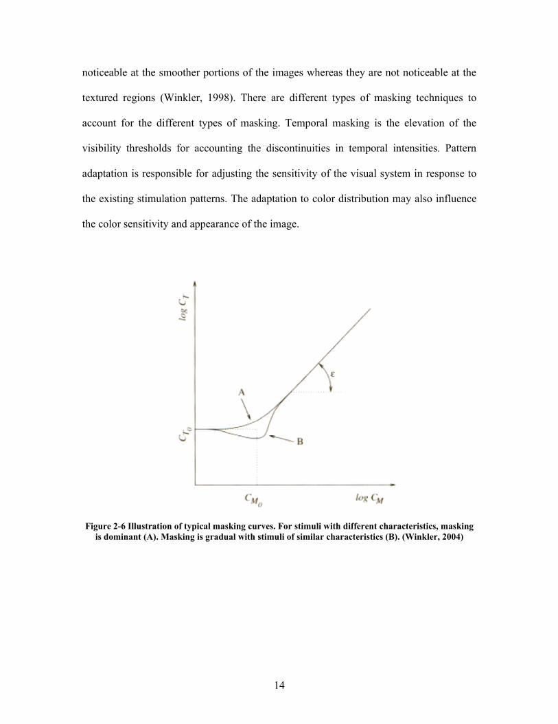
noticeable at the smoother portions of the images whereas they are not noticeable at the
textured regions (Winkler, 1998). There are different types of masking techniques to
account for the different types of masking. Temporal masking is the elevation of the
visibility thresholds for accounting the discontinuities in temporal intensities. Pattern
adaptation is responsible for adjusting the sensitivity of the visual system in response to
the existing stimulation patterns. The adaptation to color distribution may also influence
the color sensitivity and appearance of the image.
Figure 2-6 Illustration of typical masking curves. For stimuli with different characteristics, masking is dominant (A). Masking is gradual with stimuli of similar characteristics (B). (Winkler, 2004)
14

2.6 Multi-channel organization
The electrophysiological experiments of the neurons in the primary visual cortex which
are responsible for receptions showed that many of the cells did specialized functions
such as color, frequency and orientation. The measurements that were done masking and
adaptation further revealed that these stimulus characteristics are processed in different
visual pathways in the human visual system (Braddick, 1978). This is the primary basis
for the study of the multi-channel theory of the human visual system.
Figure -7 Idealized receptive field of primary visual cortex. Light and dark shades denote excitatory and inhibitory regions, respectively. (Winkler, 2004)
The human visual system is extremely complex and our current knowledge is limited to
very low-level processes. Therefore, the models based on the human visual system are
limited in scope and constitute only small part of the entire system. While the visual
system is highly adaptive, it is not equally sensitive to all stimuli. There are number of
15

inherent limitations with respect to visibility of the stimuli. The response of the visual
system depends upon the contrast patterns than on the absolute values. These
characteristics of the human visual systems were used in the design of the perceptual
quality models and metrics.
16
If you are working on something exciting that you really care about, you don't have to be pushed. The vision pulls you,
-- Steven Jobs
Digital Video Quality 3One of the greatest inventions of the twentieth century is the motion picture no matter in
whatever form it comes from, be it cinema, television or video. The enormous growth in
video processing applications and development of powerful compression techniques has
led to the move from analog to digital domain. The main goal of digital video providers is
reducing the bandwidth and storage without compromising the quality of the digital
video. This chapter will provide an overview of video compression methods and most
important digital video artifacts. Then we discuss the digital video quality measurements
and the various techniques for perceptual video quality measurements.
3.1 Video Compression
Compression is the process of reducing the redundant details in a data. Images in general
and videos in particular occupy large amounts of bandwidth and space. If the data are
17
uncompressed they can easily run into gigabytes of data, which necessitates the powerful
video compression techniques to save space and time. The generic lossless compression
algorithms are not effective for video compression as they can only achieve a data
compression ratio of 2:1. Therefore, in video compression two types of redundancy are
taken in to account: spatio-temporal redundancy and psycho visual redundancy. Spatio-
temporal redundancy exploits the fact that pixel values are correlated with the neighbors
both within the same frame and across frames. Psycho visual redundancy discards
information that is not normally observable by the viewer (Winkler, 2004).
3.1.1 Compression Methods
The digital video compression techniques are either model based methods like fractal
compression or waveform-based methods like wavelet compression. Most of the
compression techniques are waveform-based and they have three important stages of
compression.
(a) Transformation
The images are transformed to the frequency domain where different frequency ranges
with varying sensitivities to HVS can be identified. This can be reversed back to the
original domain without any loss in detail. The conversion from the original domain to
the frequency domain can be achieved through DCT or wavelet transform.
(b) Quantization
The next step after transformation is to reduce the precision of the transform coefficients
based on the number of bits for each pixel. The amount of quantization usually depends
18

upon the quality requirements of the user for example how much visible distortion the
user is able to compromise. This step is responsible for any loss in the image.
(c) Coding
Once the data has been quantized the user can encode the quantized values in the
bitstream. The fact that certain symbols occur more often than the other helps us to use
entropy encoding like Huffman or Arithmetic Coding.
3.1.2 Standards
The recent growth in multimedia applications has led to the development of number of
video compression techniques. MPEG-2 is one of the mostly used standards from DVD’s
to Digital TV and HDTV broadcast. H.263 is used for video conferencing, MPEG-1 used
in VCD’s and MPEG-4 is used in 3G mobile phones. Real Media Video, QuickTime
Video and Windows Media Video are some well-known codec’s used today.
MPEG
The international standards for multimedia compression, decompression, coding and
processing are developed and controlled by the Moving Pictures Expert Group (MPEG).
MPEG was established in 1988 since then it has produced some of the most important
video standards.
In 1992, MPEG-1 approved a standard for data storage and retrieval of motion pictures
and audio. MPEG-2, a standard for digital television was approved in 1994. The MPEG-2
19
was refinement of MPEG-1 with special consideration to interlaced sources. A standard
for multimedia applications called as MPEG-4 was approved in 1998. The main feature
of MPEG-4 was Audio-Visual Objects, an object oriented coding scheme for addressing
robustness in error-prone environments and interactive functionality for content based
access. MPEG-4 part 10 is the latest standard addressing a wide range of applications
from mobile video to HDTV.
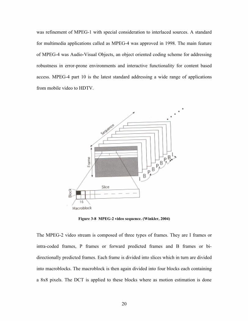
Figure 3-8 MPEG-2 video sequence. (Winkler, 2004)
The MPEG-2 video stream is composed of three types of frames. They are I frames or
intra-coded frames, P frames or forward predicted frames and B frames or bi-
directionally predicted frames. Each frame is divided into slices which in turn are divided
into macroblocks. The macroblock is then again divided into four blocks each containing
a 8x8 pixels. The DCT is applied to these blocks where as motion estimation is done
20

based on macroblocks. The resulting transform coefficients are quantized and then
variable length coding technique is applied. The transmission of data over a
communication channel is a two step process, first, the elementary streams either audio or
video are packetized which are then multiplexed together to form transport stream
(Winkler, 2004).
3.2 Video Artifacts
The compression and transmission of digital video introduce a variety of visual artifacts
into the video stream. In addition to compression and transmission, conversion between
analog and digital domain, chroma subsampling and frame rate conversion between
different types of display formats introduce visual artifacts.
Figure 3-9 Digital Video Transmission (van den Brandon, 2001)
3.2.1 Compression Artifacts
The compression algorithms used in various video coding standards are similar. Most of
them use rely on motion compensation and DCT transformation followed by quantization
for compression. In all these coding standards, the compression artifacts are induced by
quantization operation. Although other factors affect the quality of the video stream but
they do not cause distortions as quantization.
21

Figure 3-10 Illustration of artifacts due to compression (a) Original, (b) Block-DCT and (c) Wavelet, respectively. The blocking effect and staircase effect can be seen in b. Blur and ringing artifacts are
seen in both the images (Winkler, 2004).
The blocking effect or blockiness is block like pattern in the compressed sequence. The
blocking effect is the most widely noticeable artifact in a compressed sequence. Some of
the other compression artifacts are blur, color bleeding, ringing, false images, flickering
and aliasing. Though these are mostly seen in block based algorithms these artifacts are
also seen in other compression algorithms.
22

3.2.2 Transmission Artifacts
The compressed video is mostly transferred over packet-switched network. A noisy
channel can impair the video sequence which is being transmitted. The bitstream is
normally transmitted through wire or wireless channel at the physical layer and with
protocols like TCP or UDP at the transport layer. The headers of the bit streams contain
sequencing, timing and signaling information. For streaming real-time video, we need
additional protocols for decoding and displaying the information in real-time.
Figure 3-11 Illustration of video transmission system. The video sequence is first compressed using an encoder. The resulting bitstream is packetized and transmitted over the network (Winkler, 2001).
The packets may be lost or delayed during the data transmission which makes the packets
missing during decoding of the video. The quality of the video impaired based on the
frame that was lost or delayed. For example, a MPEG macroblock that was dropped or
delayed corrupts remaining macroblocks in the slice until it is resynchronized. This also
results in temporal loss propagation as those blocks that were predicted based on the
corrupted block based on motion prediction will be corrupted as well.
23
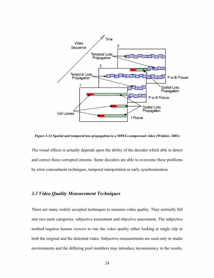
Figure 3-12 Spatial and temporal loss propagation in a MPEG-compressed video (Winkler, 2001)
The visual effects is actually depends upon the ability of the decoder which able to detect
and correct those corrupted streams. Some decoders are able to overcome these problems
by error concealment techniques, temporal interpolation or early synchronization.
3.3 Video Quality Measurement Techniques
There are many widely accepted techniques to measure video quality. They normally fall
into two main categories: subjective assessment and objective assessment. The subjective
method requires human viewers to rate the video quality either looking at single clip or
both the original and the distorted video. Subjective measurements are used only in studio
environments and the differing pool members may introduce inconsistency in the results.
24

An objective measurement for testing video quality is more reproducible and portable but
the measurement system should have good correlation with the subjective testing results
for the same data test sequences. Objective methods do not need human viewers but tries
to come up with the quality measure by manipulating the signal values using the
knowledge of the human visual system. The results of the objective results should be
consistent and correlate with the subjective benchmarks for the same data sets.
3.2.1 Subjective Quality Measurement
The subjective quality assessment techniques have been used as reliable way of assessing
video quality for many years. The subjective video quality assessment methods are
defined by the Recommendation ITU-R BT.500-10 “Methodology for the subjective
assessment of the quality of television pictures”. It is done by two types Double Stimulus
methods where reference as well as the transmitted video is presented and Single
stimulus methods where only test video is presented. Double Stimulus Continuous
Quality Scale is the most widely method where the reference as well as the test sequence
are presented. The subjects are asked to rate the test sequence based upon the reference
sequence on a continuous quality scale. In single stimulus methods only the test sequence
is presented and they are asked to rate on a five level quality scale. In Double Stimulus
Continuous Quality-Scale Method (DSCQS) the processed sequence is compared to the
original. In Single Stimulus Continuous Quality Evaluation (SSCQE) method only the
processed sequence is assessed without seeing the original one (Fenimore, 2005).
25

Figure 3-13 Typical subjective video quality assessment laboratory.
Subjective quality assessment techniques are important as it is the only way to evaluate
the performance of objective quality techniques. Though the results provided by the
subjective experiments are still efficient but they have obvious disadvantages. They are
not easily repeatable, time-consuming and cannot be automated.
26

Figure 3-14 Subjective quality assessment metrics corresponding to quality score from 1 to 5
3.2.2 Objective Quality Measurement
Objective video quality assessments of digital video can be divided into three categories.
The first method is called as full reference method where the transmitted video is
compared with the original sequence. The second method is called as the reduced
reference where the features of the original video are compared with the transmitted
frame. The third one is called as the no-reference frame where you try to estimate the
quality based on the transmitted frame only.
The full reference method can be used only in situations where you have the original
video sequences at the receiver. The advantage of full reference video is that is possible
27

to do frame by frame comparison between the original and the distorted video to arrive at
quality score. The reduced reference method can be used by transmitting the features for
comparison to the distorted video. After extracting the features from the distorted video
and we come up with the quality score based on the differences between the features. The
no-reference method is used in situations where we do not have access to the original
video or the cost of transmitting the features of the original video is expensive. Therefore,
the no-reference method is useful when the original video is not available for comparison
at the receiving end (Wang, 2004).
The normal way of estimating video quality is based on the error signal. The error is the
absolute difference between the original and transmitted signal. The traditional methods
like Mean Square Error (MSE) and Peak Signal-to-Noise Ratio (PSNR) are effective
when the error is additive but not for digital video where the signal is correlated. The
video quality estimation techniques that are developed these days are based on the human
visual system (HVS) which are based on the human observes and sees the video. The
models based on this are Perceptual distortion metric (PDM), Digital video quality
(DVQ) and Just Noticeable Difference (JND) metric.
The objective method of video quality measurements have been studied and accepted in
traditional media like television where the display and the quality range are very high.
But mobile networks where user normally user PC screens and mobile display, viewing is
from very short range, conventional methods like PSNR produce results that are quite
different from subjective measurements (Watson, 2001). This is due to the fact that
28

PSNR considers all the pixels in the image as equal whereas human perception of the
each pixel depends upon its position in the image. The full reference assessment
technique is used when the unimpaired original sequence is readily available when the
assessment is being done. There are several new objective quality assessment techniques
but there is not any one internationally recognized standard video quality assessment
technique to date. The main goal of the video industry is to provide acceptable level
video quality for the distribution video content to the customers.
3.2.3 Pixel based Quality Metrics
The mean squared error (MSE) and Peak Signal-to-Noise Ratio (PSNR) are the most
widely used difference metrics in image processing. MSE is the mean of the squared
differences between the pixel values of the two pictures. Video Quality is mostly
measured using PSNR which is defined as the difference between the peak signal and rms
noise observed between the reference and the distorted video sequence.
Equation 3-1
29

Figure 3-15 The same amount after inserting to original image (a) at two different parts of the image. (Winkler, 2004)
PSNR cannot be a reliable method of perceiving video quality because they do not take
the human visual system into account for quality estimation (Wolf, 2002). This is because
the human viewers will be able to perceive different types of distortions like blockiness,
jerkiness and noise which did not have large PSNR values.
30
Things won are done; joy's soul lies in the doing.- Shakespeare
KUIM Video Quality Pipeline 44.1 Overview
We have implemented a system to estimate video quality that simulates the visual
pathway of the Human Visual System. The perceptual distortion metric we have used is
based on a contrast gain control model of the human visual system that incorporates the
spatial and temporal aspects of vision as well as color perception (Winkler, 2004). It
considers aspects of human vision such as color perception, spatio-temporal contrast
sensitivity and multi-channel representation of human visual system. Our system requires
both the reference as well as distorted sequence as inputs. Both video streams are
converted into opponent-colors space which results in three different images. These are
then passed through the temporal weighted averaging and spatial filtering. These are done
both for the reference video as well as the transmitted video. At the final step, the sensor
differences between both the reference and distorted video sequence are calculated and
31

combined into a distortion measure. This process is illustrated in Figure 4-1. The
remainder of this chapter describes our system in more detail.
Figure 4-16 KUIM video quality pipeline block diagram
32

4.1.1 Color Space Conversion
The RGB color spaces are widely used for coding digital images but they cannot be used
for HVS based models. Since these are not perceptually linear and device dependent, we
need to convert to a color space which is perceptually linear and device independent. The
absorption rates of the three types of the cones in the retina are the only way to achieve
device independence. The cone absorption rates can be calculated based on the spectral
power distribution of light emitted from the display phosphors and the spectral
sensitivities of the cones. The color space standards such as JPEG, NTSC, and PAL take
certain properties of the human visual system into consideration by coding non-linear
color differences instead of the usual linear RGB color components. The digital video is
usually encoded in YUV color space where Y is the luminance component and the U and
V are the difference between the blue and luminance and difference between red and
luminance respectively.
Our KUIM video quality pipeline model is based on the theory of opponent colors. The
theory of opponent colors is based on the principle that the sensations of red and green as
well as blue and yellow are processed in separate visual pathways (Winkler, 2004). Some
pairs of hues can be seen as single color sensation while it is not the case for others. For
example, reddish yellow is seen as orange whereas reddish green is seen as reddish green
only. The opponent color spaces are three different channels black-white (WB), red-green
(RG) and blue-yellow (BY). The existing color spaces are providing importance to
human perception of color by providing gamma correction for the RGB color spaces. The
33

input image from the RGB color space is converted into opponent color space through a
series of transformations.
Figure 4-17 Color space conversion from RGB to Opponent color space
The input image from the RGB color space is first converted to device independent CIE
XYZ tristimulus by the following transformation defined by the ITU-R Rec BT.709-5
(2002).
Equation 4-3
The CIE XYZ tristimulus values form the basis for conversion to human visual system
related color space. The responses on the L-, M- and S-cones on the human retina are
calculated using the following transformation.
34

Equation 4-4
These LMS values can be converted to an opponent color space proposed by Poirson and
Wandell (1996). The W-B, R-G and B-Y components are computed using the LMS
values based on the following transformation.
Equation 4-5
The opponent color space was designed to separate color perception from pattern
sensitivity which has been considered an advantage of modular design of the metric. This
color space is based on color-matching experiments and not based on the human
perception of color differences. Color spaces such as CIE L*a*b and CIR L*u*v which
are widely used in other metrics are based on color differences but lack the ability to
separate pattern and color.
4.1.2 Temporal Mechanisms
The features of the temporal mechanisms in the human visual system are still under
discussion in the vision community. Temporal averaging is very important in calculating
the quality of the video signal. The quality of the video depends on the fact the moving
35

object is being tracked by the eye. In video sequences, most of the details in a video
frame are almost same as the previous frame. If a camera moves from left to right, most
part of the frame is same as the previous one except for the new part at the right side of
the frame. Temporal information gives an indication of the image changes in time
domain, for example between frame n and frame n-1. The video sequences with no
motion activity between frames will have higher video quality as the loss in quality will
not be perceived by the user. Temporal information is computed from the pixel-wise
difference between two successive frames in the video sequence. It is the indicator for the
amount of information in the video. If there are duplicate frames in a video sequence, the
difference between successive frames will be zero. We apply the temporal low-pass filter
to all the three channels based on the work by Frederickson and Hess (1998). The
temporal high pass filter increases contrast and suppresses the background of the image.
A temporal low pass filter when applied helps in anti-aliasing the image.
4.1.3 Spatial Mechanisms
The HVS is sensitive to low spatial frequencies but less sensitive to high spatial
frequencies. Therefore, the intensity and color of the image is more important than the
very fine details of the image. Spatial information gives us the number of edges in frame.
The cells in the human visual system are mostly specialized so that they are sensitive to
certain types of signal such as color, patterns or orientation. This multi-channel theory of
human visual system is basis on human perception. The model decomposes the images
into different channels based on the spatio-temporal characteristics of the human visual
36

system. The perceptual decompositions is done first in the temporal and then in the
spatial domain. We chose binomial low pass filter for the decomposition in the spatial
domain. The binomial low pass filter is based on binomial coefficients for implementing
Gaussian filtering which is most common form of linear filtering. The binomial filters
require low arithmetic operations compared to other filters by not requiring
multiplications which results in faster processing time (Aubury and Luk, 1995).
Figure 4-18 VPIPELINE program block diagram
37
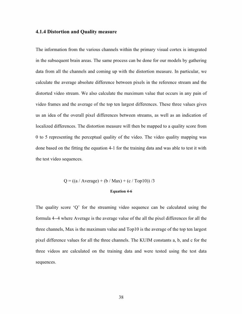
4.1.4 Distortion and Quality measure
The information from the various channels within the primary visual cortex is integrated
in the subsequent brain areas. The same process can be done for our models by gathering
data from all the channels and coming up with the distortion measure. In particular, we
calculate the average absolute difference between pixels in the reference stream and the
distorted video stream. We also calculate the maximum value that occurs in any pain of
video frames and the average of the top ten largest differences. These three values gives
us an idea of the overall pixel differences between streams, as well as an indication of
localized differences. The distortion measure will then be mapped to a quality score from
0 to 5 representing the perceptual quality of the video. The video quality mapping was
done based on the fitting the equation 4-1 for the training data and was able to test it with
the test video sequences.
Q = ((a / Average) + (b / Max) + (c / Top10)) /3
Equation 4-6
The quality score ‘Q’ for the streaming video sequence can be calculated using the
formula 4--4 where Average is the average value of the all the pixel differences for all the
three channels, Max is the maximum value and Top10 is the average of the top ten largest
pixel difference values for all the three channels. The KUIM constants a, b, and c for the
three videos are calculated on the training data and were tested using the test data
sequences.
38

Video Sequences Motion Content A B C
Woman(CW) Low 19.26 64.88 29.65
Traffic (PC) High 54.02 162.8 78.81
Man (CA) Low 17.73 61.60 22.70Table 4-1 KUIM constants for three video sequences
4.2 Implementation
During the development of the KUIM video quality pipeline three programs were written.
The AVI2JPG which converts the raw AVI files from AVI into sequences of JPEG
images for subsequent analysis. The Vsampler program is used for temporal sampling the
distorted video sequences. The most important program is Vpipeline, which implements
the main video processing pipeline for comparing two video sequences. The fourth step
is post processing of the calculated distorted measure and coming up with the VMOS
score representing video quality.
4.2.1 Preprocessing – Conversion from AVI to JPEG
The first step involves the conversion of the original video in AVI format to a sequence
of JPEG frames. The AVI files of the original as well as the distorted videos were
converted to JPEG files for video quality assessment. This was done because the KUIM
software library works for JPEG files and not AVI files. The original video which is also
called as reference sequence was converted to JPEG files with 223 frames for 6 second
streaming video. The initial blue frames are called as the synchronization frames and
39

there are sequence numbers at the bottom of each frame for alignment. This program
when given an AVI video as input skips the header details and extracts the raw
uncompressed video frames. The extracted video frames are then converted to JPEG
images using the KUIM JPEG library.
4.2.2 Temporal Sampling
The temporal sampling is done for the distorted video so that to remove any duplicates or
additional frames that may have been transmitted during video streaming. This is very
important for full reference method where we calculate the distortion measure by frame
by frame comparison. The number of frames in the reference as well as distorted videos
needs to be the same for a fair comparison. The duration of all the videos is six seconds at
25 frames per second. The reference frame has 223 frames with a frame being
transmitted every 40us. The preprocessor samples each frame based on the nearest
neighborhood method for every 40us. The timestamp for each frame along with the frame
number is obtained from the log that accompanied each frame. The log file is a text
document that has a timestamp value for each frame that was generated during test data
generation. Since our temporal sampling was based on nearest neighborhood methods we
were able to get rid of duplicate frames which does not have any effect on visual
perception where as we retain all the missing frames which account for visual quality.
After temporal sampling, the number of frames in the reference and the distortion video
are of same size. We also get rid of the initial blue frames which are used for
synchronization purposes for streaming video.
40

Figure 4-19 Vsampler Implementation
4.2.3 Video Pipeline
The video pipeline program takes the distorted video as input and reads all the images
into a queue. The images from the queue are then converted into opponent color space
resulting in three different images. The three queues for the opponent color spaces are for
the W-B channel, R-G channel and B-Y channel. The images from the all the three
channels are done temporal weighted averaging with the window size of 5.
The images from the output queue of weighted averaging are passed through binomial
spatial smoothing. These steps are done for both the reference as well as the distorted
videos. We then based on equation 4-4; calculate the differences between the reference
images and the distorted images which almost similar to user perceived difference. The
41

Figure 4-20 KUIM Perceptual Software Pipeline Implementation
42

resultant differences are then used to calculate the distortion measure and arrive at a
quality score.
The input videos, reference and the distorted video are read into two queues for
processing as KUIM_COLOR images. The queues are the instances of the
KUIM_QUEUE class and this is the first stage of Vpipeline program. The frames in the
two input queues are then converted to opponent color space resulting in three queues
each containing KUIM_SHORT images. The frames are read from the input queues until
they have no more frames in the input queue. The same color conversion is done for both
the input queues which contain the reference and distorted video frames. The six queues
after color conversion, three for each video sequence are then passed through temporal
low pass filter. The temporal low pass filter does weighted averaging on a window size of
5 with weight of 1 for all the frames.
The six output queues from the temporal low pass filter then undergoes binomial spatial
smoothing resulting in six output queues, three for the reference video and three for the
distorted video. These six videos are then compared against each other and the average of
the sum absolute differences are written to a file while the difference image is written as
JPEG output for analysis. The status of all the input queues, output queues and the
intermediate queues such as the number of frames in the queue are displayed for the user.
All the above steps are executed as pipeline as the input queue of one method depends
upon the output queue of the previous process. If there are no frames in the input queue,
43

the process has to wait till there is any frame is written into the input queue. Once there
is a frame available in an input queue, the process can remove the next available frame,
perform the necessary functions and they insert the resulting frame into the output queue.
The frame number and the timestamp are used to order the frames in the video. Each step
in the above pipeline spawn separates process for executing a particular function. This is
because though they depend on the output of their previous step, they do not have wait
till end of the previous step. They remove the frame from the input queue whenever they
are available and write the results to the output queue for further processing down the
pipeline.
4.2.4 Video Score
The video quality score is calculated after analyzing the results and distortion measure.
These values are then mapped along with the SwissQual calculated MOS to arrive at the
final quality score. The distortion measure is must be converted to a quality score that
can be compared to the MOS values obtained from NetQual. This is because the
distortion measure is the visual difference between the reference and distorted video
sequences. This can be done based on a correlation plot between the NetQual score and
the distortion measure.
44

Results! Why man, I have gotten a lot of results.I know several thousand things that won’t work.
-- Thomas Alva Edison
Testing and Results 5In this chapter, the KUIM perceptual software pipeline that introduced in Chapter 3 is
evaluated. The test video sequences and the experimental procedures are presented along
with the analysis of the performance of the metric. The analysis is based on the data
obtained from the NetQual framework. The prediction performance of the KUIM
perceptual software pipeline in comparison to the MOS scores from NetQual and other
relevant metrics.
5.1 Metrics
The concept of Mean Opinion Score was originally developed to rate the perceived
quality of voice call. The test was fully subjective with the test being done under
controlled conditions. A pool of test subjects will rate the sequence of voice calls from a
scale ranging from 1 to 5.
45
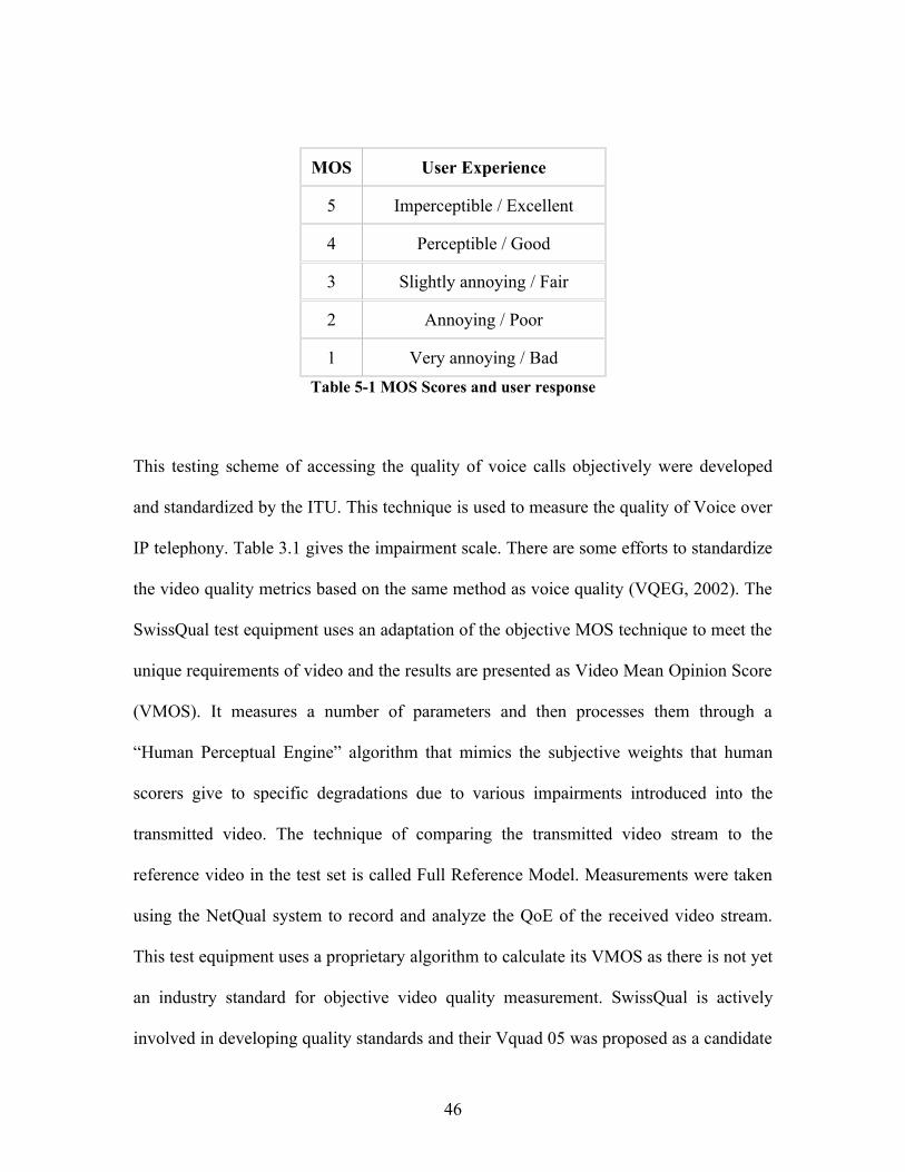
MOS User Experience
5 Imperceptible / Excellent
4 Perceptible / Good
3 Slightly annoying / Fair
2 Annoying / Poor
1 Very annoying / BadTable 5-1 MOS Scores and user response
This testing scheme of accessing the quality of voice calls objectively were developed
and standardized by the ITU. This technique is used to measure the quality of Voice over
IP telephony. Table 3.1 gives the impairment scale. There are some efforts to standardize
the video quality metrics based on the same method as voice quality (VQEG, 2002). The
SwissQual test equipment uses an adaptation of the objective MOS technique to meet the
unique requirements of video and the results are presented as Video Mean Opinion Score
(VMOS). It measures a number of parameters and then processes them through a
“Human Perceptual Engine” algorithm that mimics the subjective weights that human
scorers give to specific degradations due to various impairments introduced into the
transmitted video. The technique of comparing the transmitted video stream to the
reference video in the test set is called Full Reference Model. Measurements were taken
using the NetQual system to record and analyze the QoE of the received video stream.
This test equipment uses a proprietary algorithm to calculate its VMOS as there is not yet
an industry standard for objective video quality measurement. SwissQual is actively
involved in developing quality standards and their Vquad 05 was proposed as a candidate
46

for ITU/VQEG video quality standard competition in 2005. The objective quality
assessment results should correlate with the subjective quality assessment techniques.
5.2 Test Set-Up
The data used for evaluating the models were obtained from the Sprint ATL and the
quality rating for comparison were obtained using SwissQual’s NetQual setup. The
equipment in the lab consisted of a Helix Multi-media server, a client running NetQual
application test set and an EVDO Samsung A600 PCS Vision phone. The server was
connected directly to the SprintlLink public internet. The phone was connected to the test
set and served as a modem for the test set to access the Sprint PCS and SprintLink
production network. Video was encoded as MPEG-4, H.263 and MPEG-2 transport
streams.
47

Figure 5-21 Network Set-Up for Data Generation for Test Sequences
Both the Darwin Server and the NetQual test set have identical copies of three
uncompressed videos. Two of them are low motion videos of woman sitting outside a
café drinking water and a man talking to an interviewer; and the third one is a high
motion video of auto traffic outside Piccadilly Circus. There are sets of videos for 5, 12
and 25 frames per second for each of these. Each of these speeds has three streams
encoded at three different levels of compression 1. Video base layer only, 2. Base plus
video enhanced layer, 3. Base plus additional enhanced layer. The Darwin server uses
QuickTime 6.5.1 MPEG-4, H.263 encoder. Enhanced video information requires more
bits per second to be transmitted, but the resulting video quality will be increased. This
48

technique of copying a video from the test set and comparing with the transmitted video
received from the streaming server is called as Full Reference Model.
5.3 Video Sequences
In order to evaluate the proposed quality metrics, we chose source sequences to cover a
wide range of typical content for mobile applications such as low motion and high motion
content. Three scenes with different frame rate of 25 Hz and resolution of 176 x 144
pixels were used for data collection.
Figure 5-22 Reference Test Sequences (a) Woman (b) Car and (c) Man
The high motion sequence shows auto traffic outside Piccadilly Circus (PC) has a
significant amount of spatial detail, a considerable amount of fast motion and slow
camera movement, which makes it ideal testing sequence for spatio-temporal vision. The
other video sequences are of low motion content with a woman drinking water outside a
café (CW) and interview with a man (CA). Each sequence has duration of six seconds.
49

The sample frame from each scene can be found in Figure 5.1. The video sequence was
encoded as MPEG-4 and H.263 streams over MPEG-2 transport streams.
SEQUENCES MOTION CONTENT SEQUENCE NAME VMOS
Car High PC_2.6_45_009008 2.6
Woman Low CW_2.7_45_005005 2.7
Car High PC_3.1_45_004008 3.1
Car High PC_3.7_45_001008 3.7
Car High PC_3.7_45_002008 3.7
Car High PC_3.7_45_003008 3.7
Car High PC_3.7_45_005008 3.7
Car High PC_3.7_45_006008 3.7
Car High PC_3.7_45_007008 3.7
Car High PC_3.7_45_008008 3.7
Car High PC_3.7_45_010008 3.7
Woman Low CW_4.1_45_001005 4.1
Woman Low CW_4.1_45_002005 4.1
Woman Low CW_4.1_45_003005 4.1
Woman Low CW_4.1_45_004005 4.1
Woman Low CW_4.1_45_006005 4.1
Woman Low CW_4.1_45_007005 4.1
Woman Low CW_4.1_45_008005 4.1
Woman Low CW_4.1_45_009005 4.1
Woman Low CW_4.1_45_010005 4.1
50

Man Low CA__4.4_45_001009 4.4
Man Low CA__4.4_45_002009 4.4
Man Low CA__4.4_45_003009 4.4
Man Low CA__4.4_45_004009 4.4
Man Low CA__4.4_45_005009 4.4
Man Low CA__4.4_45_006009 4.4Table 5-2 Test Video Sequences
5.4 Results
The performance of the objective quality assessment techniques should be done with
results from the subjective measurements. Since the main goal of this study was to
identify an objective assessment technique which provides the same results as subjective
measurements, we used SwissQual results for comparison. Subjective ratings for the
resultant test sequences were obtained using the NetQual software from SwissQual. The
ratings were used to compare the performance of the KUIM perceptual software pipeline.
The performance of our KUIM perceptual software pipeline can be evaluated based on a
statistical analysis of the correlation of its predictions with the NetQual VMOS for the
same set of video sequences.
51

Figure 5-23 Reference, Distorted and Pixel Differences for Woman, Car and Man test sequences in RGB Color Space
To evaluate the performance of KUIM perceptual software pipeline we used three
different video sequences, two of which are low motion content and third is contains high
motion content. The distorted video sequences were generated using the Sprint EVDO-
Rev 0 mobile network and NetQual application set-up. A sample frame from each
sequence and its distorted version along with the pixel wise differences in RGB color
space can be found in Figure 5.3.
52

The W-B, R-G and B-Y components of the opponent color space after conversion from
the RGB color space are shown in Figure 5.4. You can see the emphasis of red color in
the R-G channel for the PC test video sequence and the emphasis of yellow leaves in B-Y
component in CW test sequence. The W-B component which encodes luminance
information of the image is almost like the grey level representation of the image.
Figure 5-24 W-B, R-G and B-Y components of the test sequences after opponent color conversion for Woman, Car and Man test sequences, respectively
The color space conversions are then followed by temporal weighted averaging in the
quality pipeline model. The W-B, R-G and B-Y components of the distorted sequences
53

are after temporal weighted averaging can be seen in Figure 5-5. The temporal weighted
averaging was done the test video sequences with window size of five and this was done
to reduce the temporal aspects of the distortions. The window can of any size but the best
results were obtained in the range from 5 to 10 to remove distortions that depend on the
neighboring frames.
Figure 5-25 W-B, R-G and B-Y components of the test sequences after temporal weighted averaging for Woman, Car and Man test sequences, respectively
All the same components after going through the binomial spatial smoothing process in
pipeline are shown in Figure 5-6. The binomial spatial smoothing reduces the sharpness
54
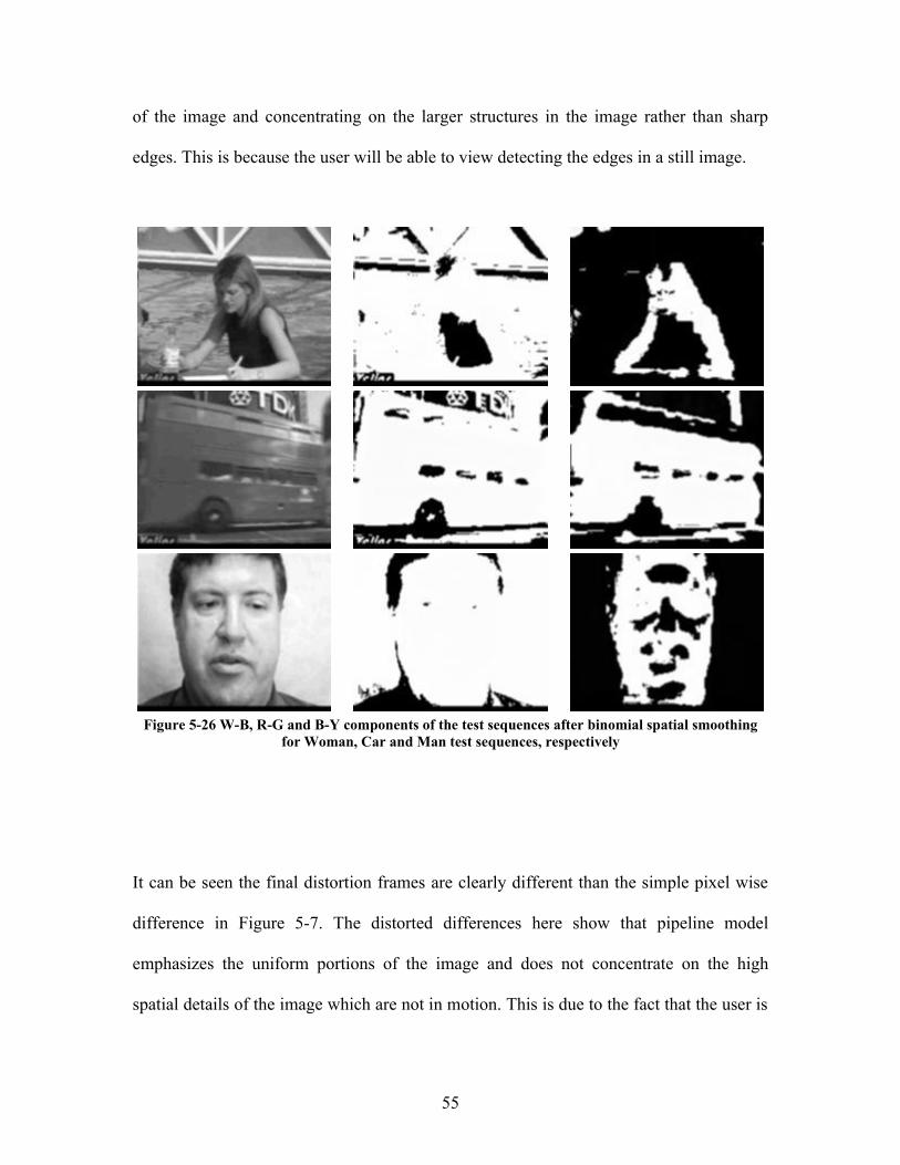
of the image and concentrating on the larger structures in the image rather than sharp
edges. This is because the user will be able to view detecting the edges in a still image.
Figure 5-26 W-B, R-G and B-Y components of the test sequences after binomial spatial smoothing
for Woman, Car and Man test sequences, respectively
It can be seen the final distortion frames are clearly different than the simple pixel wise
difference in Figure 5-7. The distorted differences here show that pipeline model
emphasizes the uniform portions of the image and does not concentrate on the high
spatial details of the image which are not in motion. This is due to the fact that the user is
55
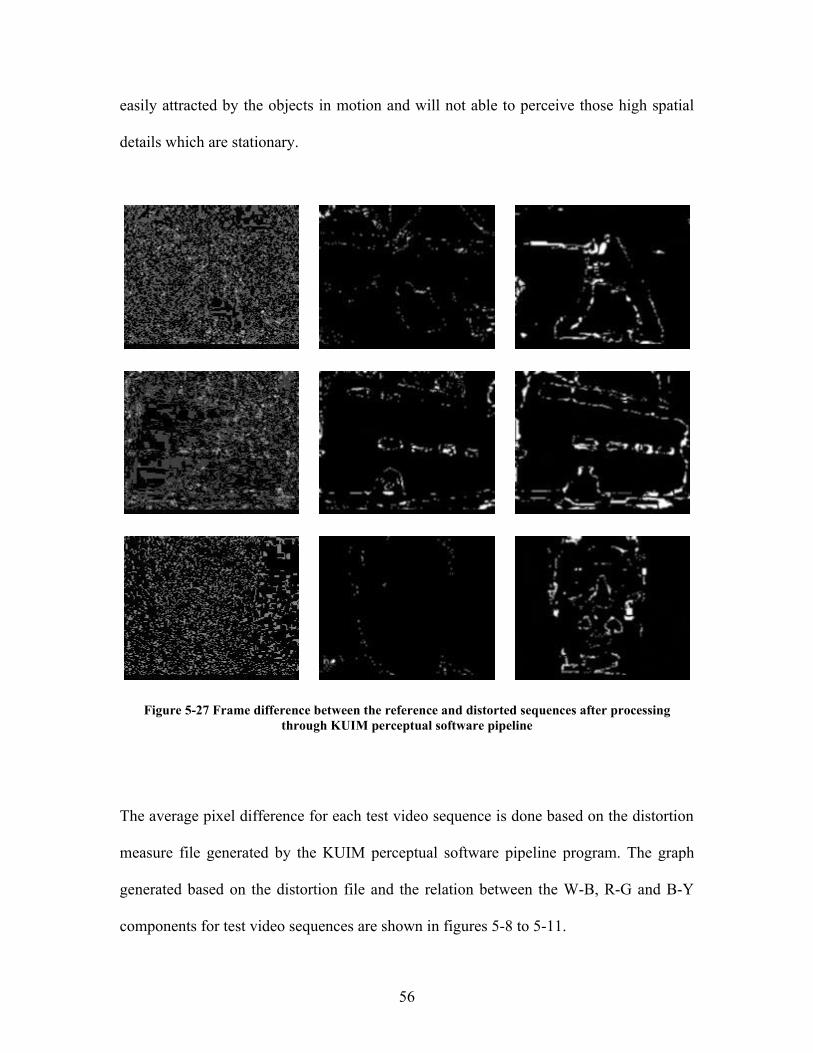
easily attracted by the objects in motion and will not able to perceive those high spatial
details which are stationary.
Figure 5-27 Frame difference between the reference and distorted sequences after processing through KUIM perceptual software pipeline
The average pixel difference for each test video sequence is done based on the distortion
measure file generated by the KUIM perceptual software pipeline program. The graph
generated based on the distortion file and the relation between the W-B, R-G and B-Y
components for test video sequences are shown in figures 5-8 to 5-11.
56

Average Pixel Difference in Opponent Color Space
0
5
10
15
20
25
30
0 50 100 150 200 250
Frame
Ave
rage
Pix
el D
iffer
ence
W-BR-GB-Y
Figure 5-28 Average pixel difference between the reference and distorted sequence for Woman
Average Pixel Difference in Opponent Color Space
020406080
100120140160180
0 50 100 150 200 250
Frame
Ave
rage
Pix
el D
iffer
nce
W-BR-GB-Y
Figure 5-29 Average pixel difference between the reference and distorted sequence for Car
57

Average Pixel Difference in Opponent Color Space
02468
10121416
0 20 40 60 80 100 120 140 160 180
Frame
Ave
rage
Pix
el D
iffer
ence
W-BR-GB-Y
Figure 5-30 Average pixel difference between the reference and distorted sequence for Man
The pipeline parameters such as the maximum value, average of top ten values, and
average of W-B, R-G and B-Y are calculated and the results are plotted as graph in
figures 5-11 to 5-13. This was done for all the three different video sequences.
KUIM Pipeline parameters
0
5
10
15
20
25
30
1 2 3 4 5 6 7 8 9 10
Test Video Sequences
MOS AverageMaxTop10W-BR-GB-Y
Figure -31 KUIM Pipeline parameters for Woman
58
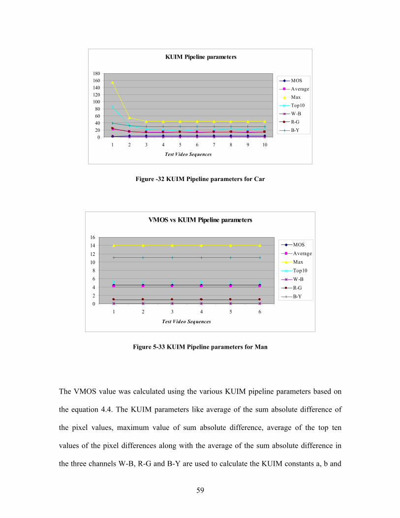
KUIM Pipeline parameters
020406080
100120140160180
1 2 3 4 5 6 7 8 9 10
Test Video Sequences
MOS AverageMaxTop10W-BR-GB-Y
Figure -32 KUIM Pipeline parameters for Car
VMOS vs KUIM Pipeline parameters
02468
10121416
1 2 3 4 5 6
Test Video Sequences
MOS AverageMaxTop10W-BR-GB-Y
Figure 5-33 KUIM Pipeline parameters for Man
The VMOS value was calculated using the various KUIM pipeline parameters based on
the equation 4.4. The KUIM parameters like average of the sum absolute difference of
the pixel values, maximum value of sum absolute difference, average of the top ten
values of the pixel differences along with the average of the sum absolute difference in
the three channels W-B, R-G and B-Y are used to calculate the KUIM constants a, b and
59
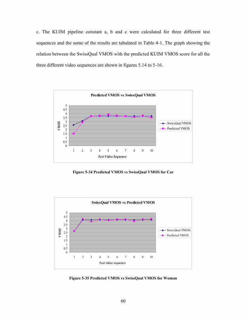
c. The KUIM pipeline constant a, b and c were calculated for three different test
sequences and the some of the results are tabulated in Table 4-1. The graph showing the
relation between the SwissQual VMOS with the predicted KUIM VMOS score for all the
three different video sequences are shown in figures 5.14 to 5-16.
Predicted VMOS vs SwissQual VMOS
00.5
11.5
22.5
33.5
44.5
5
1 2 3 4 5 6 7 8 9 10
Test Video Sequence
VMOS SwissQual VMOS
Predicted VMOS
Figure 5-34 Predicted VMOS vs SwissQual VMOS for Car
SwissQual VMOS vs Predicted VMOS
00.5
11.5
22.5
33.5
44.5
5
1 2 3 4 5 6 7 8 9 10
Test video sequence
VM
OS SwissQual VMOS
Predicted VMOS
Figure 5-35 Predicted VMOS vs SwissQual VMOS for Woman
60

Predicted VMOS vs SwissQual VMOS
00.5
11.5
22.5
33.5
44.5
5
1 2 3 4 5 6
Test Video Sequence
VMOS SwissQual VMOS
Predicted MOS
Figure 5-36 Predicted VMOS vs SwissQual VMOS for Man
The results from figures 5-14, 5-15 and 5-16 show that KUIM perceptual software
pipeline is able to predict the VMOS score equivalent to the SwissQual VMOS score for
most of the test video sequences. It can be seen the results of the KUIM perceptual
software pipeline are consistent with the NetQual MOS scores.
VIDEO SEQUENCES
MOTION CONTENT
SEQUENCE NAME
SWISSQUALVMOS
PREDICTEDVMOS
Woman Low CW_2.7_45_005005 2.7 2.70
Woman Low CW_4.1_45_001005 4.1 4.20
Woman Low CW_4.1_45_002005 4.1 3.92
Woman Low CW_4.1_45_003005 4.1 4.17
Woman Low CW_4.1_45_004005 4.1 4.02
Woman Low CW_4.1_45_006005 4.1 4.16
Woman Low CW_4.1_45_007005 4.1 4.17
Woman Low CW_4.1_45_008005 4.1 3.91
Woman Low CW_4.1_45_009005 4.1 4.17
Woman Low CW_4.1_45_010005 4.1 4.21Table 5-2 SwissQual VMOS vs Predicted VMOS - Woman
61

VIDEO SEQUENCES
MOTION CONTENT
SEQUENCE NAME
SWISSQUALVMOS
PREDICTEDVMOS
Car High PC_2.6_45_009008 2.6 1.48
Car High PC_3.1_45_004008 3.1 2.91
Car High PC_3.7_45_001008 3.7 3.66
Car High PC_3.7_45_002008 3.7 3.72
Car High PC_3.7_45_003008 3.7 3.90
Car High PC_3.7_45_005008 3.7 3.72
Car High PC_3.7_45_006008 3.7 3.67
Car High PC_3.7_45_007008 3.7 3.55
Car High PC_3.7_45_008008 3.7 3.72
Car High PC_3.7_45_010008 3.7 3.49Table 5-3 SwissQual VMOS vs Predicted VMOS - Car
VIDEO SEQUENCES
MOTION CONTENT
SEQUENCE NAME
SWISSQUALVMOS
PREDICTEDVMOS
Man Low CA__4.4_45_001009 4.4 4.39
Man Low CA__4.4_45_002009 4.4 4.39
Man Low CA__4.4_45_003009 4.4 4.39
Man Low CA__4.4_45_004009 4.4 4.39
Man Low CA__4.4_45_005009 4.4 4.39
Man Low CA__4.4_45_006009 4.4 4.39Table 5-4 SwissQual VMOS vs Predicted VMOS - Man
62
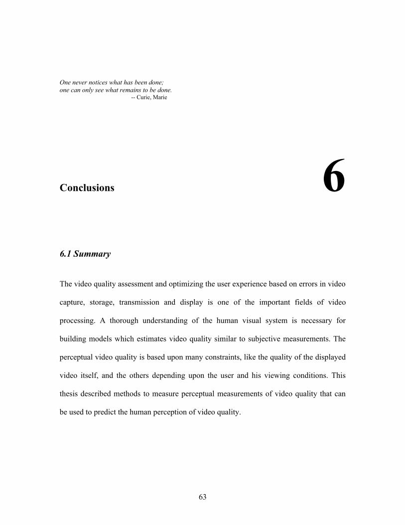
One never notices what has been done; one can only see what remains to be done.
-- Curie, Marie
Conclusions 66.1 Summary
The video quality assessment and optimizing the user experience based on errors in video
capture, storage, transmission and display is one of the important fields of video
processing. A thorough understanding of the human visual system is necessary for
building models which estimates video quality similar to subjective measurements. The
perceptual video quality is based upon many constraints, like the quality of the displayed
video itself, and the others depending upon the user and his viewing conditions. This
thesis described methods to measure perceptual measurements of video quality that can
be used to predict the human perception of video quality.
63

6.2 Areas of further research
One of the potential areas of research is calculating the visual quality without any
reference frames. This will greatly reduce the need to transmit the original frame for
video quality estimation and it will also help to enhance the quality of the video in real-
time without any user feedback. This also helps us to rate the quality of the video in a
non-intrusive way without the knowledge of the user. This has great advantages in
commercial applications as we will be able the assess the video quality without user
intervention if we can able to package the application along with user mobile phone or
PDA.
As pointed out by VQEG, the reduced reference model of calculating visual quality is
very useful in situations where we cannot transmit the original sequence. This will help
us to transmit the essential features for comparison and to arrive at a quality score rather
than transmitting the whole sequence and there by saving bandwidth and time.
The quality of the video also depends upon the audio that plays along with it. So focusing
on the quality metrics for both audio and video will the direction to pursue further
research. Moreover, the visual quality depends upon number factors which make it
necessary for experts in psychophysics, vision science and video processing to work
together for best possible solution.
64

Great discoveries and achievements invariably involve the cooperation of many minds.
-- Alexander Graham Bell
References
[ 1 ]Aubury, M., Luk, W. (1995). Binomial Filters. Journal of VLSI Processing, pp. 1-
16.
[ 2 ]Braddick, O., Campbell, F. W., Atkinson, J. (1978). Channels in vision: Basic
aspects. In Held, R., Leibowitz, H., Teuber, H. L.(eds), Perception, vol. 8 of
Handbook of Sensory Physiology, pp. 3-38, Springer-Verlag.
[ 3 ]Fenimore (2005). Subjective testing methodology in MPEG video verification.
Available at http://www.nist.gov/
[ 4 ]Furht, B., Marqure, O., (2003). Chapter 41 in The Handbook of Video Databases:
Design and Applications. CRC Press.
[ 5 ]Guyton, A. C. (1991). Textbook of Medical Physiology, 7th edn, W. B. Saunders.
[ 6 ]Han, J., Ngan, K. N., Li, M., Zhang, H. (2006).unsupervised extraction of visual
attention objects in color images. IEEE Transactions on Circuits and Systems for
Video Technology, vol. 16, no. 1.
[ 7 ]Hering, E. (1878). Zur Lehre vom Lichtsinne, Carl Gerolds.
[ 8 ]Hood, D. C., Finkelstein, M. A. (1986). Sensitivity to light. In Boff, K. R., Kaufman,
L., Thomas J. P.(eds), Handbook of Human Perception and Performance, vol. 1,
chap. 5, John Wiley.
65

[ 9 ]ITU-R Recommendation BT.500-11 (2002). Methodology for subjective assessment
of the quality of television pictures. ITU, Geneva, Switzerland.
[ 10 ]ITU-R Recommendation P.910 (1999). Subjective video quality assessment
methods for multimedia applications. ITU, Geneva, Switzerland.
[ 11 ]Javůrek, R. (2004). Efficient models for objective video quality assessment.
Radioengineering, vol. 13, no. 4.
[ 12 ]Kelly, K. (2002). Quality of Service In Internet Protocol (IP) Networks.
International Communications Industries Association.
[ 13 ]Marimont, D. H., Wandell, B. A. (1994). Matching color images: The effects of
axial chromatic aberration. Journal of the Optical Society of America 11(12): 3113-
3122.
[ 14 ]Poirson, A. B., Wandell, B. A. (1996). Pattern color separable pathways predict
sensitivity to simple colored patterns. Vision Research 36(4):515-526.
[ 15 ]Stockman, A., Sharpe, L. T. (2000). Spectral sensitivities of the middle- and long-
wavelength sensitive cones derived from measurements in observers of unknown
genotype. Vision Research 40(13):1711-1737
[ 16 ]Verscheure, O., Frossard, P., Hamdi, M. (1999). Real-Time Imaging. Available
online at http://www.idealibrary.com
[ 17 ]VQEG (2000). Current Results and Future Directions. Available at
http://www/vqeg.org
[ 18 ]VQEG (2000). Final Report from the Video Quality Experts Group on the
validation of objective models for video quality assessment. Available at
http://www/vqeg.org
66
[ 19 ]VQEG (2003). Final Report from the Video Quality Experts Group on the
validation of objective models for video quality assessment - Phase II. Available at
http://www/vqeg.org
[ 20 ]Watson, A. B., & Kreslake, L. (2001). Measurement of visual impairment scales for
digital video. Proceedings of the SPIE, vol. 4299, 79-89.
[ 21 ]Watson, A. B., Hu, J., & McGowan, J. F., III. (2001). Digital video quality metric
based on human vision. Journal of Electronic Imaging, 10(1), 20-29.
[ 22 ]Watson, A. B., Hu, J., McGowan III, J. F.(2001). Digital Video Quality metric
based on human vision. Journal of Electronic Imaging 10(1), pp. 20-29.
[ 23 ]Westheimer, G. (1986). The eye as an optical instrument. In Boff, K. R., Kaufman,
L., Thomas J. P.(eds), Handbook of Human Perception and Performance, vol. 1, chap.
4, John Wiley.
[ 24 ]Winkler, Stefan. (1998). A perceptual distortion metric for visual color images. In
Proc. International Conference on Image Processing, vol. 3, pp. 399-403, Chicago,
IL.
[ 25 ]Winkler, Stefan (2005). Digital Video Quality: vision models and metrics. John
Wiley.
[ 26 ]Wolf, S., Pinson, M. H. (2002). Video Quality Measurement Techniques. NTIA
Report 02-392.
[ 27 ]Yang, F., Wan, S., Chang, Y., Wu H. R. (2005). A Novel Objective No-Reference
Metric for Digital Video Quality Assessment. IEEE Signal Processing Letters, vol.
12, no. 10.
67

[ 28 ]Young, R. A. (1991). Oh say, can you see? The Physiology of vision. In Proc. SPIE
Human Vision, Visual Processing and Digital Display, vol. 1453, pp. 92-9123, San
Jose, CA.
68