pdf - arxiv.org · 2 maury bramson, bernardo d’auria, and neil walton in our setting, queues will...

PROPORTIONAL SWITCHING IN FIFO NETWORKS

MAURY BRAMSON, BERNARDO D’AURIA, AND NEIL WALTON

Abstract. We consider a family of discrete time multihop switched queueing networks where each packet movesalong a fixed route. In this setting, BackPressure is the canonical choice of scheduling policy; this policy has

the virtues of possessing a maximal stability region and not requiring explicit knowledge of traffic arrival rates.

BackPressure has certain structural weaknesses because implementation requires information about each route,and queueing delays can grow super-linearly with route length. For large networks, where packets over many

routes are processed by a queue, or where packets over a route are processed by many queues, these limitations

can be prohibitive.In this article, we introduce a scheduling policy for FIFO networks, the Proportional Scheduler, which is

based on the proportional fairness criterion. We show that, like BackPressure, the Proportional Scheduler hasa maximal stability region and does not require explicit knowledge of traffic arrival rates. The Proportional

Scheduler has the advantage that information about the network’s route structure is not required for scheduling,

which substantially improves the policy’s performance for large networks. For instance, packets can be routedwith only next-hop information and new nodes can be added to the network with only knowledge of the

scheduling constraints.

1. Introduction

We consider, in this paper, a family of discrete time multihop switched queueing networks where packetsmove along fixed routes. Switched networks were first introduced in Tassiulas and Ephremides (1992); thisterminology was first employed in Shah and Wischik (2012) for a discrete time queueing network whose queuesare served simultaneously subject to certain global scheduling constraints and with packets moving along fixedroutes. Here, we consider a variant of this model that allows more than one route through each queue; thescheduling constraints and queueing discipline employed here do not depend on the routes of the packets.

Applications of switched networks include wireless ad-hoc networks, Internet routers, call centers with crosstrained staff, data centers, and urban road traffic scheduling. For such applications, and in general, maximumstability is a highly desirable feature for the scheduling policy. Roughly stated, for switched networks, ascheduling policy is maximally stable if, for every arrival rate for which there exists a stable policy, the policystabilizes the network. When the vector of arrival rates is known, one can specify a stable policy by choosing arandom schedule whose average service rate at each queue dominates the corresponding arrival rate. However,in practice, explicit knowledge of arrival rates is often not available, particularly when rates may vary. Sincethe seminal work of Tassiulas and Ephremides (1992), BackPressure has been the canonical maximally stablescheduling policy for multihop switched networks. An important feature of this policy is that, in addition to itbeing maximally stable, only information on the local state is required for a scheduling decision.

When packets are routed through different network components, policies such as BackPressure require de-tailed knowledge of this routing. Such policies are similar in nature to the classical single class Jackson queueingnetworks if one identifies each route with a queue, so that each queue now contains only a single customer type.However, in many applications, this single class interpretation may not be practical because the informationrequired can increase rapidly in the number of queues of the original network. It is also not common practice– for instance, an Internet router will maintain a first-in, first-out (FIFO) queue for each outgoing link ratherthan a queue for each route, because the number of links to and from a router is orders of magnitude smallerthan the number of routes it processes. As a result, in many practical situations, the model simplifies if onereinterprets queues as being multiclass, i.e., permitting different packet classes and hence different routing ofpackets passing through the queue.

Key words and phrases. Proportional Scheduler, BackPressure, Kelly networks, bandwidth sharing networks, Massoulie net-works, switch networks, proportional fairness.

The research of the first author was partially supported by NSF grants DMS-1105668 and DMS-1203201.

The research of the second author was partially supported by the Spanish Ministry of Economy and Competitiveness GrantsMTM2013-42104-P via FEDER funds; he thanks the ICMAT (Madrid, Spain) Research Institute that kindly hosted him while

developing this project.

The research of the first author was partially supported by NSF grants DMS-1105668 and DMS-1203201. The research of thesecond author was partially supported by the Spanish Ministry of Economy and Competitiveness Grants MTM2013-42104-P via

FEDER funds; he thanks the ICMAT (Madrid, Spain) Research Institute that kindly hosted him while developing this project.The research of the third author was funded by the VENI research programme, which is financed by the Netherlands Organisationfor Scientific Research (NWO).

1

arX

iv:1

412.

4390

v3 [

mat

h.PR

] 2

1 Ju

l 201

6

2 MAURY BRAMSON, BERNARDO D’AURIA, AND NEIL WALTON

In our setting, queues will be multiclass but will serve packets according to a scheduling policy allocatingservice among queues that depends only on the number of packets at each queue; the discipline at each queuewill be FIFO and packets will all be of unit size. In this setting, we will show that this switching policy, theProportional Scheduler, is maximally stable.

There are well-known examples of disciplines that are not maximally stable for multiclass queues, for instance,Lu and Kumar (1991), Rybko and Stolyar (1992) and Bramson (1994). (These examples are in both discreteand continuous time.) The examples in Bramson (1994) are for the FIFO discipline, with jobs having unequalmean service requirements. In switch networks, all jobs have equal service requirements and so do not fallwithin this framework.

Our policy, the Proportional Scheduler, can be described roughly as follows: for a set of FIFO queues J ,

a vector of queue lengths (Qj : j ∈ J ) ∈ Z|J |+ , and a convex set of schedules < S >⊂ R|J |, the Proportional

Scheduler serves packets according to a vector of expected rates, σ ∈ R|J |, that solves the proportional fairoptimization problem

maximize∑j∈J

Qj log σj over σ ∈<S> .(1)

Packets within a queue are to be served according to a FIFO queueing discipline; once served, a packet goes tothe next queue on its route.

We prove that maximal stability holds for this policy by employing a fluid model analysis of our system. Thiscombines the approaches of Massoulie (2007), for bandwidth networks, and Bramson (1996), for FIFO Kellynetworks; the latter networks can be viewed as the special case of switched networks where the allocation ofservice to different queues is fixed irrespective of the state of the system.

We also compare our policy to the BackPressure policy. Unlike BackPressure, the Proportional Schedulerdoes not require knowledge of the route used by each packet. Thus, routing structure and scheduling decisionsare distinct for the Proportional Scheduler policy. As we later discuss in more detail, there are various benefitsof the Proportional Scheduler’s functional structure: a) rather than distinguishing packets according to theirroutes (either in the memory of the scheduling algorithm or by physically maintaining different queues), packetscan be served at their queue in a first-in, first-out order, b) a packet can be routed knowing only its next hop,rather than knowing its entire route, c) when adding new network components, one only needs to know thecomponent’s scheduling constraints and not the entire route or class structure of the network to implement thepolicy, and d) for BackPressure, messages must be sent between queues, which the Proportional Scheduler doesnot require.

On the other hand, the Proportional Scheduler policy is less general than BackPressure in that the lattermodel allows for adaptive routing decisions whereas routing for the Proportional Scheduler is fixed.

Another well-known switched network policy is the MaxWeight policy; it is defined by the optimization whoseobjective function employs the linear factor σj , in place of log σj , in (1), i.e.,

maximize∑j∈J

Qjσj over σ ∈<S> .(2)

As such, it also satisfies the properties a) – d) above. MaxWeight is maximally stable for single hop networks,since it coincides there with the BackPressure policy.

MaxWeight is not always maximally stable for multihop networks, even when each queue possesses onlyone class. This is shown in Andrews and Zhang (2003) for fluid models for a weighted version of MaxWeight,after modifying the model slightly by varying the arrival rate of mass; supporting simulations are then givenfor a queueing network under the standard MaxWeight policy. We briefly consider the maximal stability ofMaxWeight in Section 3, but leave a detailed investigation of the policy to future work.

The same question about maximal stability exists for policies with objective functions employing factorsother than σj or log σj . As the counterexample in Andrews and Zhang (2003) shows, care needs to be exercisedin the choice of the objective function in (1).

1.1. Relevant Literature. The main results of this paper combine a number of results, methods, and modelsfrom the theory of queueing networks over the last three decades. We review this relevant literature in a roughlychronological order.

A. Classical Queueing Networks: The development of Jackson networks is one of the earliest substantialdevelopments in the theory of stochastic networks. In Jackson networks, a single class of customers is routedprobabilistically between queues in the network. Influenced by the Input Theorem of Burke (1956), Jackson(1963) found that the stationary distribution of these networks can be written in product form, meaning thatits stationary distribution is the product of simple terms.

Baskett et al. (1975) and Kelly (1975, 1979) broadened this family of queueing networks by permitting queuesto be multiclass, and hence allowing more than one route through each queue. Using quasi-reversibility, they

PROPORTIONAL SWITCHING 3

showed that, for certain service disciplines including FIFO, the stationary distribution must be of product form.(Quasi-reversibility will also be employed in the context of proportional fairiness in Part D below.)

B. Switched Networks, BackPressure and their Applications: Switched queueing networks and, more specifi-cally, the BackPressure scheduling policies, were first introduced by Tassiulas and Ephremides (1992) as a modelof wireless communication. As mentioned above, a switched queueing network is a discrete time queueing net-work with constraints on which queues can be served simultaneously. The BackPressure policies have provenpopular because they maximize a network’s stability region while not requiring explicit estimation of trafficarrival rates; for a comprehensive review of the BackPressure policies, see Georgiadis et al. (2006).

The BackPressure policies have been generalized and specialized in numerous directions. In contrast to ourwork, the defining feature of a BackPressure policy is that the policy minimizes the drift of a Lyapunov functionsubject to the scheduling constraints of the network. For single hop networks – where packets are served onlyonce before departing the network – the BackPressure policy is often referred to as the MaxWeight policy. As amodel of Internet protocol routers, McKeown et al. (1999) applied this paradigm to the example of input-queuedswitches. Andrews et al. (2004) consider power functions when defining their MaxWeight Lyapunov function andthus generalized the set of MaxWeight/BackPressure policies. Additional extensions are considered by Meyn(2009) and Eryilmaz et al. (2005) and further generalizations to cone polices are considered by Armony andBambos (2003). In different stochastic senses, BackPressure and MaxWeight can be shown to optimize certainworkload functions: in heavy traffic, see Stolyar (2004); in large deviations, see Venkataramanan and Lin (2007);in overload, see Shah and Wischik (2011). Further, heavy tailed arrivals are analyzed by Jagannathan et al.(2011); delay in the presence of heavy tailed traffic are considered in Markakis et al. (2014).

There are numerous application areas associated with switched networks. For these areas, BackPressure isoften the canonical choice. Applications include wireless ad-hoc networks, in Tassiulas and Ephremides (1992),Internet routers, in McKeown et al. (1999), call centers with cross trained staff, in Mandelbaum and Stolyar(2004), data centers, in Shah and Wischik (2011), urban road traffic scheduling, in Varaiya (2013), and stochasticprocessing networks, which would include numerous manufacturing and general processing settings, in Dai andLin (2005).

C. Instability, Fluid Stability and Stability of Queueing Networks: Most classical queueing networks arepositive recurrent when the network is subcritical. By positive recurrent, we mean that there exists a state(which, in our setting, will be the state with no packets) that is positive recurrent and that this state is visitedwith probability 1 starting from any other state; this is the reduction to the countable state space setting ofpositive Harris recurrence, which is the standard definition in the general state space setting. By subcritical,we mean that each network resource experiences a load that is strictly less than the resource’s capacity. It hadbeen thought that subcritical networks were always positive recurrent under a work conserving policy. However,a series of examples constructed in the mid-nineties showed that this is not the case. For instance, see Lu andKumar (1991), Rybko and Stolyar (1992) and Bramson (1994).

This led to new approaches for determining the stability region for queueing networks. In particular, Rybkoand Stolyar (1992) and Dai (1995) developed a fluid model approach where the stability of a queueing networkcan be determined from that of an associated fluid model. This theory is surveyed in by Bramson (2008). Afluid analysis of multiclass FIFO queueing networks was first given by Bramson (1996). Our fluid analysis usesa similar approach.

Recent work of Dieker and Shin (2013) further considers the issue of finding natural scheduling policies thatlead to stability whenever each server is nominally underloaded. Similar to adversarial queueing frameworks,e.g., Borodin et al. (2001), stability is achieved by prioritizing queue service according to a least-routed-first-priority discipline. This differs from the approach taken in this paper where the service discipline does notuse the routing structure of the network to achieve maximum stability. Further recent work of Ji et al. (2013)considers stability results for switched networks where packets are queued per-link rather than per-route, asis typically applied for BackPressure. Here stability is achieved by running an appropriate queueing systemin the memory of the algorithm. By estimating queue sizes and loads in this way, stability is achievable forswitched networks as long as routes do not form a loop. Once again this differs from the approach of thispaper, where routes are general and only current queue size information is required to execute the schedulingpolicy. Finally, Ying et al. (2011) consider a modification of the BackPressure policy to lessen the effect ofper-route queueing. Queues are grouped into predetermined clusters, with the standard BackPressure policyapplied within each cluster. A judicious choice of clusters will reduce the amount of required memory. Clustersare centrally determined and, as with BackPressure, per-link queueing is not employed and information on thequeue size must be continuously exchanged along queues between the source and destination.

D. Massoulie Networks, Proportional Fairness and Quasi-Reversibility: A further class of Internet modelswas introduced in Massoulie and Roberts (1999) and Massoulie and Roberts (2000) in a processor-sharingframework where resources are shared subject to constraints on these resources. Similar to MaxWeight andBackPressure, these policies are often defined by an optimization that is maximally stable. (Unlike BackPressure,the construction does not minimize the instantaneous drift of a Lyapunov function.) Stability proofs for thesesystems can be found in Bonald and Massoulie (2001), Ye et al. (2005), Gromoll and Williams (2009) and


Paganini et al. (2012). Due to their proliferation to different areas, these models have taken various names,such as bandwidth sharing networks, stochastic flow level models, and resource sharing networks; here, we referto these networks as Massoulie networks. See Harrison et al. (2014) for a recent discussion of the benefits andvaried applications of this resource sharing paradigm.

In this paper, we allocate resources according to the proportional fair optimization, which was first introducedby Kelly (1997). Proportional fairness has been used in the allocation of bandwidth in modern 3G telephonenetworks, see, e.g., Viswanath et al. (2002) and Kushner and Whiting (2004). The stability of proportionalfairness in Massoulie networks was first shown by De Veciana et al. (1999); an important generalization of thisstability analysis is given in Massoulie (2007). Further progress on the stability and large deviations behavior ofproportional fairness can be found in Jonckheere and Lopez (2014). Heavy traffic analysis of proportional fairpolicies can be found in Kang et al. (2009), Ye and Yao (2012), and Vlasiou et al. (2014). Stolyar (2004) hasinvestigated resource pooling for MaxWeight policies. Kang et al. (2007), Kang et al. (2009), Kelly et al. (2009)and Ye and Yao (2012) discussed product form resource pooling properties associated with the proportionalfairness in heavy traffic and large deviations regimes.

Influenced by Whittle (1985), the quasi-reversibility and insensitivity property in Massoulie networks wasstudied by Bonald and Proutiere (2002, 2003, 2004) and Zachary (2007). For connections between proportionalfairness and the queueing networks of Kelly (1975) and Baskett et al. (1975), see, e.g., Schweitzer (1979); Kelly(1989); Massoulie and Roberts (1999); Walton (2009), and Anselmi et al. (2013). A short, general descriptionof the relationship between proportional fairness, maximum stability and quasi-reversibility can also be foundin Walton (2011). As we discuss later, the Lyapunov function in Massoulie (2007) is relevant to our analysis.

E. Resource Sharing in Switched Networks: The sharing of network resources is a key property of theproportional fair optimization. Other resource sharing policies exist, e.g., the weighted α-fair policies of Moand Walrand (2000). Only recently, authors have begun to consider these policies in the context of switchednetworks; to the best of our knowledge, application of α-fairness to switched networks was first made by Shahand Wischik (2011) and Zhong (2012). (Added in revision: Li and Srikant (2016) has shown stability of aper-link scheduling policy for multihop networks.)

1.2. Organization. The remainder of the paper is organized as follows. In Section 2, we define a family ofFIFO switched networks and the Proportional Scheduler. The main result of the paper, Theorem 1, statesthat the corresponding network is positive recurrent for all subcritical arrival rates. In Section 3, we discuss theproperties of the Proportional Scheduler in comparison to BackPressure; the section is not needed to understandTheorem 1, but it is important in order to understand its consequences. In Section 4, we prove Theorem 1.We begin by characterizing the fluid model that is associated with the Proportional Scheduler and then, in(20-22) and Proposition 1, define a Lyapunov function for the fluid model and calculate its derivative. This isapplied, in Theorem 2, to prove fluid stability, from which we conclude, in Proposition 3, that the correspondingstochastic network is positive recurrent. Proposition 3 and certain other steps in the proof of Theorem 1 willbe proved in the appendix.

2. FIFO Network Model, Proportional Scheduler, and Main Result

2.1. Network and Scheduling Set Notation. Let J be a finite set of queues, with cardinality |J | and

indexed by j. A schedule is a vector σ = (σj : j ∈ J ) ∈ Z|J |+ , where Z|J |+ denotes the non-negative integers.We will denote by S a finite set of schedules satisfying: (1) If σ ∈ S, then σ ∈ S for each σ ≤ σ (withvector inequalities σ ≤ σ being interpreted componentwise, i.e., σj ≤ σj for all j ∈ J ). Note that the vectorof all zeros belongs to S. (2) For each j ∈ J , there exists some schedule σ ∈ S such that σj > 0. For a

vector Q = (Qj : j ∈ J ) ∈ ZJ+ , we denote by SQ the schedules in S with σj ≤ Qj for j ∈ J , and denote byσmax := max{σj : j ∈ J ,σ ∈ S} the maximum component in the set of schedules. We define <S> to be theconvex combination of points in S and assume that <S> has non-empty interior. The subcritical region C ofthis network is the interior of <S >. (In the setting of multiclass queueing networks with a fixed service rateat each queue, <S> becomes a rectangle with faces parallel to the axes.)

Each packet in the network is assumed to belong to a class at a given time t. The notation of a packet’sclass will be used to uniquely identify the route of the packet, the queue it is at, and the stage along its route.We denote by K the set of classes of packets in the network. A route through the network is a vector of classesr = (kri : i = 1, . . . , |r|) ∈ K|r|, with size |r| ∈ N. Each class is assumed to occur along a unique route, with theclass occurring exactly once along its route; R denotes the set of routes through this network.

With each class k ∈ K, we associate a unique route denoted r(k) and a unique queue j(k). For notationalconvenience, we add an additional “outside’’ class denoted by ω: For each class k ∈ K, we let the functionb(k) ∈ K∪ {ω} denote the class before class k on route r; if k is the first class on a route, we then set b(k) = ω.Similarly, the function n(k) ∈ K∪{ω} will denote the next class on route r. If k ∈ K is the last class on a route,then n(k) = ω.

For a given route r ∈ R, we define the input class i(r) ∈ K to be the first class on route r, i.e., i(r) = kr1,and the output class o(r) ∈ K to be the last class on route r, i.e., o(r) = kr|r|. The subsets of input and output


classes are denoted by Ki and Ko, respectively. For notational convenience, we write k ∈ j to indicate that classk is at queue j, i.e., j(k) = j, and k ∈ r to indicate that class k occurs on route r, i.e., r(k) = r. Unless statedotherwise, | · | denotes the L1 norm.

2.2. Network Quantities and Equations. Our principal objects of interest are discrete time FIFO networksand the Proportional Scheduler, which are described here and in the next subsection. We begin by introducingthe state primitives for first-in, first-out (FIFO) networks having time index t ∈ Z+. Analogous primitives andequations will be employed in Section 4 for the corresponding fluid model, where time will instead be continuousand the model will be both continuous and deterministic.

Throughout the paper, the indices j, k, r will be used to refer to, respectively, queues J , classes K and routesR. Regardless of the index x = j, k, r, we will denote by Ax(t) the cumulative number of arrivals by time t, byDx(t) the cumulative departures by time t, and by Qx(t) the queue size at time t. For example, Aj(t) is thetotal number of arrivals at queue j by time t, Dk(t) is the total number of packets that have departed fromclass k, and Qr(t) is the number of packets that have arrived at but not departed from route r. For each k ∈ Kand s ∈ N, the function Γk(s) denotes the number of packets of class k that will be served after s packets areserved from queue j(k).

The processes Ax(t), Dx(t) and Γk(t) are non-negative and non-decreasing, with Ax(0) = Dx(0) = Γk(0) = 0for x ∈ J ∪ K ∪ R and k ∈ K. The queue size process Qx(t) is non-negative for x ∈ J ∪ K ∪ R. Given thesenatural conditions, the following fundamental equations hold for a FIFO switched network.

Qx(t) = Qx(0) +Ax(t)−Dx(t),(3) ∑k∈j

Γk(t) = t,(4)

(Dj(t)−Dj(s)

t− s: j ∈ J

)∈<S> for t > s,(5)

Dk(t) = Γk(Dj(t)),(6)

Ak(t) +Qk(0) = Γk(Aj(k)(t) +Qj(k)(0)),(7)

Ak(t) = Db(k)(t),(8)

where x ∈ J ∪ K ∪ R, j ∈ J , k ∈ K and r ∈ R for (3-7), and k ∈ K\Ki in (8). Finally, we define thearrivals/departures for routes by

Ar(t) = Ai(r)(t), Dr(t) = Do(r)(t).(9)

The above equations (3-8) can be interpreted as follows: (3) is standard, (4) states that the tth packetserved from queue j is from class k ∈ j, and (5) states that the departure process must be achievable within theconstraints of the network scheduling. In (6), Γk(Dj(t)) is the number of class k packets served after Dj(t) unitsof service; (7) states that all of the packets that were originally at class k or arrived there by time t will havebeen served after Aj(t) +Qj(0) packets have been served at j and so, if the Aj(t)th packet arrival is of class k,then the (Aj(t) +Qj(0))th packet departure is also of class k, i.e., the queueing discipline is FIFO; (8) gives therouting between classes. Further relationships can also be deduced from the above equations. For instance, (4)and (7) imply Aj(t) =

∑k∈j Ak(t) and Dj(t) =

∑k∈j Dk(t), and (3), (9) and (8) imply Qr(t) =

∑k∈r Qk(t).

We remark that, when the service rates σj are constant, the FIFO property given by (7) is equivalent tothe FIFO property (2.5) in Bramson (1996). The FIFO condition there is given in terms of the workload atthe queue; such an interpretation of workload does not immediately transfer to our setting, since service ratescan vary. Also note that (7) does not restrict the order in which packets that have arrived simultaneously at aqueue are served; we shall allow any such order.

In addition to equations (3-8), we also assume that the number of arrivals at each route r over different timesis i.i.d. with mean ar ∈ (0,∞), and that the arrivals at different routes occur independently. For each classk ∈ r, we set ak = ar, and for each queue j ∈ J , we set aj =

∑k∈j ak, with a = (aj : j ∈ J ). We assume

that the time required for the service of each packet is deterministic and equal to 1. With this in mind, we saythat the mean arrival vector a is subcritical for a given network when a ∈ C; observe that, since C is open, thisimplies that (1 + ε)a ∈ C for some ε > 0. This provides a natural extension to the definition of subcriticalityused for multiclass queueing networks (with a fixed allocation of service for each queue).

We note that for a network with the FIFO property, one needs to specify the initial state of the systemby including Γk(s), for 0 ≤ s ≤ Qj(0), in order to uniquely specify the corresponding Markov process. Asmentioned above, one also needs to define a tie-breaking rule when two or more packets from different classesarrive at a queue at the same time, for which we specify in the functions Γk which packet arrived “first”.

2.3. Proportional Scheduler. A scheduling policy is a sequence of schedules π(t) ∈ S with π(t) ≤ Q(t)component-wise that determines the service of packets at each queue, i.e., D(t) − D(t − 1) = π(t). The


Proportional Scheduler, which is the main focus of this paper, is defined as follows. For Q = (Qj : j ∈ J ) ∈ Z|J |+ ,let σ(Q) = (σj(Q) : j ∈ J ) ∈<S> be a solution to the following optimization problem:

maximize∑j∈J

Qj log σj over σ ∈<SQ>;(10)

when Qj = 0, set σj(Q) = 0, with the convention that 0 log 0 = 0. (Note that Q 7→ σ(Q) is invariant underscalar multiplication, i.e., σj(cQ) = σj(Q) for c > 0.) The solution to this optimization need not belong tothe set of schedules S. However, since σ ∈< SQ >, σ can be expressed as a convex combination of points inSQ, i.e., there exists random π(Q) = (πj(Q) : j ∈ J ), with support in S and such that, for j ∈ J ,

(11a) Eπj(Q) = σj(Q).

The Proportional Scheduler is defined to be any policy having the sequence of schedules π(t), where

(11b) σ(t) = arg max∑j∈J

Qj(t− 1) log σj over σ ∈<SQ(t−1)>

and π(t) satisfies the analog of (11a). (The only sources of randomness in the paper are the choice of π in (11a)and the random exogenenous arrivals Ar(t) in (9).)

Note that σ(t) is uniquely defined because of the strict concavity of the objective function in (10) and becauseσj(t) = 0 when Qj(t) = 0, although π(t) need not be uniquely defined (depending on S). Also note that theProportional Scheduler (and MaxWeight) policies reduce to the FIFO policy of a multiclass queueing network,having a fixed service rate at each queue, when <S> is a rectangle with faces parallel to the axes.

We will refer to any discrete time Markov chain satisfying the FIFO switched network equations (3-8), alongwith the policy in (11) and the arrival and service assumptions in the next to last paragraph of Subsection 2.2,as a proportional switched network. The state space of the Markov chain is assumed to be that induced by thenumber of packets at each queue together with their respective ordering within the queue. (With a slight abuseof terminology, we blur here the distinction between the Markov chain and the underlying switched network.)Recall that positive recurrent means that there exists a state (here, the state with no packets) that is positiverecurrent and that this state is visited with probability 1 starting from any other state. (This is the reductionto the countable state space setting of positive Harris recurrence from the general state space setting.)

2.4. Main Result. A standard fact is that, under any policy, a queueing network cannot be positive recurrentwhen the vector of arrival rates a lies outside the network’s subcritical region C. It follows that C is the network’sgreatest possible stability region. The main result in this paper is the following converse, which shows that theProportional Scheduler achieves its greatest possible stability region.

Theorem 1. Suppose that the vector of arrival rates a = (aj : j ∈ J ) ∈ C. Then the corresponding proportionalswitched network is positive recurrent.

Although this paper considers only proportional switched networks in the discrete time context, we remarkthat the analogous model can be defined in continuous time, with packets instead requiring an exponentialamount of service and the policy being updated immediately after each change in the state of the network.The proof of Theorem 1 relies on the application of fluid models to the proportional switched network and isinsensitive to whether time is discrete or continuous, and so will carry over to the continuous time setting. Asin the context of FIFO multiclass queueing networks, the main requirement for proportional switched networkson their service times is that their means be the same for different classes at the same queue, although themeans may differ among different queues. In our setting, the assumption that service times are all of unit sizeat different queues is due to the setting of switched networks, rather than intrinsic mathematical requirementsfor Theorem 1.

As is the case for proportional switched networks, the well-known BackPressure networks are also positiverecurrent for all subcritical arrival rates. In the next section, we will compare the implementability of the twomodels.

3. Comparison with the BackPressure

The BackPressure policy is currently the canonical policy for scheduling in multi-hop switched networks.Here, we present examples to illustrate practical differences between this policy and the Proportional Scheduler.This section is not required for the remainder of the paper.

3.1. Definition of BackPressure. We define and briefly describe the BackPressure policy using the notationintroduced in Section 2, with the reader being referred to Tassiulas and Ephremides (1992) for a more detaileddescription of the policy and its properties. The network is defined there in terms of a directed graph, but thereader can easily check that the definition we give below is equivalent; this alternative format is employed toavoid unnecessary complications. (Note that queues j ∈ J are referred as links in Tassiulas and Ephremides(1992), and classes are referred to as queues there.)


For a given buffer size distribution Q = (Qk : k ∈ K), the BackPressure policy can be defined as follows:

(1) For each queue j ∈ J , introduce the weights

(12) wj(Q) = maxk∈j

{Qk −Qn(k)

},

with Qn(k) = 0 for n(k) = ω. Denote by k∗j (Q) one of the classes where the above maximization isachieved.

(2) Over the set of schedules S, solve the optimization

(13) σ∗(Q) ∈ arg maxσ∈S

∑j∈J

σjwj(Q) .

(3) When wj(Q) > 0, schedule σ∗j (Q) packets from class k∗j (Q) at queue j ∈ J and no packets from any ofthe other classes at j during the next time increment; when wj(Q) ≤ 0, do not schedule any packets atthe queue.

Assuming that the number of arrivals of packets at each route over different times is i.i.d. and the arrivalsat different routes occur independently, then the BackPressure policy is positive recurrent whenever the arrivalrates are subcritical. This is shown by employing a quadratic Lyapunov function; the BackPressure policy, infact, maximizes the negative drift of the Lyapunov function.

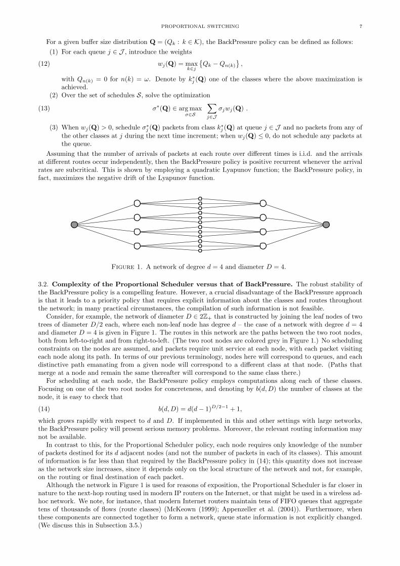
Figure 1. A network of degree d = 4 and diameter D = 4.

3.2. Complexity of the Proportional Scheduler versus that of BackPressure. The robust stability ofthe BackPressure policy is a compelling feature. However, a crucial disadvantage of the BackPressure approachis that it leads to a priority policy that requires explicit information about the classes and routes throughoutthe network; in many practical circumstances, the compilation of such information is not feasible.

Consider, for example, the network of diameter D ∈ 2Z+ that is constructed by joining the leaf nodes of twotrees of diameter D/2 each, where each non-leaf node has degree d – the case of a network with degree d = 4and diameter D = 4 is given in Figure 1. The routes in this network are the paths between the two root nodes,both from left-to-right and from right-to-left. (The two root nodes are colored grey in Figure 1.) No schedulingconstraints on the nodes are assumed, and packets require unit service at each node, with each packet visitingeach node along its path. In terms of our previous terminology, nodes here will correspond to queues, and eachdistinctive path emanating from a given node will correspond to a different class at that node. (Paths thatmerge at a node and remain the same thereafter will correspond to the same class there.)

For scheduling at each node, the BackPressure policy employs computations along each of these classes.Focusing on one of the two root nodes for concreteness, and denoting by b(d,D) the number of classes at thenode, it is easy to check that

(14) b(d,D) = d(d− 1)D/2−1 + 1,

which grows rapidly with respect to d and D. If implemented in this and other settings with large networks,the BackPressure policy will present serious memory problems. Moreover, the relevant routing information maynot be available.

In contrast to this, for the Proportional Scheduler policy, each node requires only knowledge of the numberof packets destined for its d adjacent nodes (and not the number of packets in each of its classes). This amountof information is far less than that required by the BackPressure policy in (14); this quantity does not increaseas the network size increases, since it depends only on the local structure of the network and not, for example,on the routing or final destination of each packet.

Although the network in Figure 1 is used for reasons of exposition, the Proportional Scheduler is far closer innature to the next-hop routing used in modern IP routers on the Internet, or that might be used in a wireless ad-hoc network. We note, for instance, that modern Internet routers maintain tens of FIFO queues that aggregatetens of thousands of flows (route classes) (McKeown (1999); Appenzeller et al. (2004)). Furthermore, whenthese components are connected together to form a network, queue state information is not explicitly changed.(We discuss this in Subsection 3.5.)


3.3. Simulations for a Modification of the Network of Figure 1. In Figure 2, we provide simulations forthe average total queue size for a modification of the network in Figure 1. Specifically, rather than immediatelyexiting from the root node at the end of its route, a packet returns to this node a geometric number of times,each time with probability 1− δ, δ ∈ (0, 1], before finally exiting from the network. (We could instead stipulatethat the packet returns to the node a fixed number of times before exiting.)

0.0 0.2 0.4 0.6 0.8 1.0

Load

0

20

40

60

80

100

Avera

ge t

ota

l queue s

ize

MaxWeight

BackPressure

Proportional Scheduler

Figure 2. Total queue size of MaxWeight, BackPressure, Proportional Scheduler under arange of loads.

For this modified network, the load at a root node is a(1 + 1/δ) if a is the external arrival rate at each rootnode, and so a(1 + 1/δ) < 1 is an obvious necessary condition for positive recurrence of the network, whereas,for both BackPressure and the Proportional Scheduler, the condition is sufficient by Tassiulas and Ephremides(1992) and Theorem 1. For parameters (D, d, δ) = (4, 4, 0.4142), we simulated in Figure 2 three policies,BackPressure, the Proportional Scheduler, and MaxWeight, over a range of loads. Our simulations indicatethat, as expected, BackPressure and the Proportional Scheduler are maximally stable, whereas, consistent withthe examples of input-queued switches in Andrews and Zhang (2003), MaxWeight is not.

We note that the MaxWeight has a stability region that is approximately 75% of the total capacity. (δ = .4142,

which is about√

2 − 1, was chosen so that value would not be close to 1.) In fact, MaxWeight will lose upto 50% of the capacity for networks of this type; as mentioned in the introduction, more detail on MaxWeightwill be provided in a future work. We also note that, under all loads measured in Figure 2, the average totalqueue size for the Proportional Scheduler was found to be somewhat smaller than that for BackPressure. Wewill discuss this relationship for another family of networks in Section 3.4.

3.4. Delay on Long Routes. As illustrated in Subsection 3.2, the complexity of the BackPressure policy is anissue when there are many routes. Other complications might also arise, even when all packets have the sameroute. Consider, for example, the network in Figure 3, which is a special case of the linear networks consideredby Bui et al. (2011) (in Theorem 2) and Stolyar (2011), for the BackPressure policy.

In this example, there are J ≥ 2 links in series, with packets entering at link 1 and being sequentiallyprocessed through links 1, 2, . . . , J ; there are no constraints preventing simultaneous service at different linksand, once served, a packet moves to the next link along its route. Arrivals at queue 1 occur according to aBernoulli process, with mean parameter a > 0, and one packet is served per unit time at each nonempty queue.Bui et al. (2011) and Stolyar (2011) showed that, if the network is subcritically loaded with 1/2 < a < 1, then,under the BackPressure policy, the sum of the expected queue sizes in equilibrium grows quadratically in J ,that is,

(15)

J∑j=1

E[Qj]≥ c J2

for some constant c > 0 not depending on J . Since one unit of time is required to serve each packet at a queue,it is immediate from (15) that the flow delay for packets satisfies the same lower bound.


1 2 3 J-1 J

Figure 3. (Above) A linear net-work with J links. Each packetmust pass through each link.

Figure 4. (Right) Queuelengths for the linear networkwith J = 20 links.

(on the right)

0 5 10 15 20

Link index

0

2

4

6

8

10

12

14

16

18

Avera

ge q

ueue s

ize

BackPressure with Poisson arrivals

BackPressure with Bernoulli arrivals

Proportional Scheduler with Poisson arr.

Proportional Scheduler with Bernoulli arr.

The basic idea behind the demonstration of (15) is that BackPressure only serves a packet on the jth linkwhen Qj−Qj+1 > 0, which will occur in equilibrium with probability a (since the average arrival and departurerates are equal), whereas, in equilibrium, Qj −Qj+1 ≥ −1 must always hold (since service from queue j occursonly when Qj − Qj+1 > 0). Since a > 1/2, there will be linear growth in the expected size of successivequeues from the last queue QJ to the first queue Q1, which implies the quadratic growth in J of the sum ofthe expected queue sizes. In general, when routing is more involved, one should expect the sum of the queuesizes in equilibrium to grow quadratically with route length for routes with close to critical arrival rates since,as before, BackPressure will not serve links with a negative queue size differential. (For details, see Bui et al.(2011) or Stolyar (2011).)

The Proportional Scheduler (as well as any other work conserving scheduler) will exhibit completely differentbehavior for this linear network since there are no constraints preventing simultaneous service at different links.In equilibrium, queue 1 will have either 1 or 0 packets corresponding to whether or not an arrival occurred inthe last time slot. Therefore, the output of a queue is a Bernoulli process that is independent of the currentstate of the queue. Arguing inductively, this implies that the queue sizes at different queues are independent,and hence that the sum of the queue sizes for the network is binomially distributed with parameters J anda. Consequently, under the Proportional Scheduler policy, the sum of the expected value of the queue sizes inequilibrium grows only linearly in J , with

(16)

J∑j=1

E[Qj]

= aJ.

The above reasoning that was employed for (16) is an elementary variant of Burke’s Output Theorem (as in,e.g., Burke (1956) or Hsu and Burke (1976)).

In Figure 4, we have simulated the linear network in Figure 3, with J = 20 queues, and assuming an arrivalrate of 0.6 of packets into the network and a maximal service rate of 1 at each node. In addition to the caseof Bernoulli input discussed above, Poisson input is also simulated for both BackPressure and the ProportionalScheduler. As expected from the above discussion, for BackPressure, the average queue size is proportional tothe number of hops from the terminal destination while, for the Proportional Scheduler, the average queue sizeis constant; in neither of these cases, is the average queue size sensitive to the distribution of the input exceptfor the first few links, as illustrated by the almost perfect overlay of the pairs of graphs. It follows that, as thelength of the linear network grows, queueing delay grows quadratically for BackPressure and linearly for theProportional Scheduler. (Similar observations were made in the simulations conducted by Bui et al. (2011).)

3.5. Decomposition. Decomposition is essential to the decentralized implementation of a policy. A propertyof BackPressure optimization is that, once queue length comparisons have been made between links (see (12)),the optimization can be decomposed. In particular, if the scheduling of one subset of queues J1 does not effectthe scheduling choice of a complementary subset J2 (i.e., S = S1 × S2), then the BackPressure optimizationcan be decomposed as

maxσ∈S

{∑j∈J

σjwj(Q)}

= maxσ∈S1

{ ∑j∈J1

σjwj(Q)}

+ maxσ∈S2

{ ∑j∈J2

σjwj(Q)}.

The sub-problems involving the two optimizations on the right can then be solved independently, leading to adecomposed implementation of the policy. We remark, however, that the above optimization may not completely


decompose since the weight calculations wj(Q) typically require comparisons with the sizes of upstream queues,and hence some information exchange will occur between network components.

No such queue size comparisons are required for the proportional fair optimization that is employed to definethe Proportional Scheduler, and so the optimization can be completely decomposed as

maxσ∈<S>

{∑j∈J

Qj log σj

}= maxσ∈<S1>

{ ∑j∈J1

Qj log σj

}+ maxσ∈<S2>

{ ∑j∈J2

Qj log σj

}for complementary components having independent scheduling. This leads to more potential applications whenthe network decomposes, in comparison with the BackPressure policy.

4. Maximum Stability Proof

In this section, we prove Theorem 1, for which we employ fluid model techniques introduced in Dai (1995).The basic idea is to show that the Markov chain converges under appropriate scaling to a deterministic fluidmodel, and then to show that the queue lengths of all normalized fluid model solutions converge to 0 withina fixed time. This latter step requires most of the work in the proof and is shown by defining an appropriateLyapunov function that decreases to 0 by this time.

From a mathematical point of view, the main contribution of this argument is the extension of fluid modeltechniques to a case with varying service speeds. Here, this requires identifying the Lyapunov function in (22),showing it to be non-increasing in Corollary 2, and then showing that this Lyapunov function in fact decreasesat a fixed rate by applying Lemmas 3 and 8. The proofs of certain technical lemmas and propositions arerelegated to the appendix.

4.1. Fluid Model. We will employ, in Section 4, a fluid model, with the functions Ax(t), Dx(t), Qx(t), andΓk(t), that satisfies the same conditions (3-8) as the discrete time switched network of Section 2, and such thatAx(t), Dx(t) and Γk(t) are non-negative and non-decreasing, and Qx(t) is non-negative, with Ax(0) = Dx(0) =Γk(0) = 0 for x ∈ J ∪ K ∪ R and k ∈ K. Note that each of the conditions (3-8) is invariant under the “law oflarge numbers” scaling, where both time and space are scaled equally.

In addition to these conditions, the route arrival and queue departure processes of the fluid model will beassumed to satisfy

Ar(t) =art,(17)

Qj(t) > 0 implies D′j(t) = σj(Q(t)) ,(18)

for given ar > 0 and for t > s > 0, j ∈ J and r ∈ R, with σ(Q) denoting a solution to the proportional fairoptimization

(19) σ(Q) ∈ arg maxσ∈<S>

∑j∈J

Qj log σj .

As in Section 2, we set σj(Q) = 0 whenever Qj = 0 and, for each class k ∈ r and queue j ∈ J , set ak = ar,aj =

∑k∈j ak, and a = (aj : j ∈ J ). We will refer to the conditions (3-8) and (17-19) on A(t), D(t), Q(t), and

Γ(t) as proportional switch fluid model equations, or collectively, as the proportional switch fluid model (or fluidmodel, for short).

Together, the above conditions imply with a little work that, for x ∈ J ∪K∪R, the components Ax(t), Dx(t),Qx(t), and Γx(t) are all Lipschitz continuous and thus almost everywhere differentiable. Note that D′j(t) = 0need not hold when Qj(t) = 0, since work may enter and leave an empty queue of a fluid model. Also note thata solution of the fluid model equations corresponding to a given initial condition need not be the unique suchsolution.

4.2. Lyapunov Function and its Derivative. In this subsection, we define the entropy function H(t) andprove that it has negative derivative for non-empty subcritical systems. We first introduce the functions

L(t) =∑j∈J

Qj(t) logD′j(t),(20)

M(t) =∑j∈J

∑k∈j

∫ Qj(0)+Aj(t)

Dj(t)

Γ′k(s) logΓ′k(s)

akds;(21)

H(t) is then defined as

(22) H(t) = L(t) +M(t) .

The entropy function H(t) builds on entropy functions in Massoulie (2007) and Bramson (1996). The term L(t)is derived in Massoulie (2007) as the large deviations rate function of a reversible network that approximatesproportional fairness; the term M(t) is similar to the entropy function employed in Bramson (1996) for FIFOmulticlass queueing networks.


The function L(t) is well defined everywhere (with, as earlier, the convention that 0 log 0 = 0). Note that

Qj(t) = Qj(0) +Aj(t)−Dj(t) =∑k∈j

(Γk(Qj(0) +Aj(t))− Γk(Dj(t)))

=∑k∈j

∫ Qj(0)+Aj(t)

Dj(t)

Γ′k(s) ds ;

(23)

the lower and upper bounds Dj(t) and Qj(0) +Aj(t) for the integral in (23) can be thought of as the amountsof packet mass having departed from the queue j by time t and having departed by the later time when the lastof the mass already at j at time t departs from the queue. With (23) in mind, note that M(t) is the sum overthe different queues of a weighted version of the packet mass at each queue j at time t, based on the departurerates of the mass at the queues.

The following lemma shows that the function H(t) is always non-negative for any solution of the fluid model.

Lemma 1. For any t ≥ 0, H(t) ≥ 0. Moreover, whenever the arrival rate vector a belongs to the interior ofthe scheduling set C, then H(t) = 0 iff Q(t) = 0.

Proof. Proof By (23),

Qj(t) log aj =∑k∈j

∫ Qj(0)+Aj(t)

Dj(t)

Γ′k(s) log aj ds

for each j ∈ J ; adding and subtracting such terms allows one to rewrite H(t) as

(24) H(t) =∑j∈J

∫ Qj(0)+Aj(t)

Dj(t)

∑k∈j

Γ′k(s) log

(Γ′k(s)

ajak

)ds+

∑j∈J

Qj(t) logD′j(t)

aj.

By Jensen’s inequality,

(25)∑k∈j

Γ′k(s) log

(Γ′k(s)

ajak

)= −

∑k∈j

Γ′k(s) log

(1

Γ′k(s)

akaj

)≥ − log

∑k∈j

Γ′k(s)1

Γ′k(s)

akaj

= 0.

From this, it follows that the first summation in (24) is non-negative. The non-negativity of the second term in(24) follows since the service rates D′j(t) solve the optimization problem (19) and a ∈ C, and so, in particular,∑

j∈JQj(t) logD′j(t) ≥

∑j∈J

Qj(t) log aj .

Together with (25), this implies H(t) ≥ 0.When the fluid model is subcritical, one can improve on the inequality in the last display to show that H(t)

is positive when Q(t) 6= 0. For this, note that a ∈ C implies the existence of an ε > 0 such that

(1 + ε)a ∈ C .

Since D′(t) is an optimal scheduling, it follows that, for Q(t) 6= 0,

(26)∑j∈J

Qj(t) logD′j(t)

aj≥∑j∈J

Qj(t) log(1 + ε) > 0 .

Consequently, H(t) = 0 implies Q(t) = 0. Trivially, Q(t) = 0 implies H(t) = 0. �

We next show that H(t) is decreasing when Q(t) 6= 0, by proving H ′(t) is negative. Since we do not know in

advance that L(t) is sufficiently regular to apply the Fundamental Theorem of Calculus to∫ tsL′(u) du, we will

employ the following technical lemma, which is based on Lemma 5 of Massoulie (2007).

Lemma 2. There exists a time T > 0 not depending on the initial queue state such that:i) For t ≥ T |Q(0)|,

(27) L′(t) =∑j∈J

Q′j(t) logD′j(t) a.e.

ii) There exists a constant κL > 0 such that, for all t ≥ s ≥ 0,

(28) L(t)− L(s) ≤ κL(t− s).

iii) For all t ≥ s ≥ T |Q(0)|,

L(t)− L(s) ≤∫ t

s

L′(u) du.


A proof of this lemma is given in the Appendix.Since the processes A(t) and D(t) are Lipschitz, it is easy to see that the term M(t), which integrates an a.e.

bounded function, is Lipschitz and hence a.e. differentiable. Thus, the following corollary is immediate fromLemma 2.

Corollary 1. i) There exists a constant κH > 0 such that, for t ≥ s ≥ 0,

(29) H(t)−H(s) ≤ κH(t− s).

ii) There exists a time T > 0 not depending on the initial state such that H(t) is a.e. differentiable ont ∈ [T |Q(0)|,∞) and, for given s, t with t ≥ s ≥ T |Q(0)|,

(30) H(t)−H(s) ≤∫ t

s

H ′(u) du.

We now focus on computing H ′(t). The following proposition shows that H ′(t) is the sum of two terms:the (unnormalized) relative entropy between route departure and arrival rates, and the (unnormalized) relativeentropy between queue arrival and departure rates. This decomposition will play an important role in the proofof Theorem 2.

Proposition 1. For T as in Corollary 1, and t ≥ T |Q(0)|,

(31) H ′(t) = −∑r∈R

D′r(t) logD′r(t)

A′r(t)−∑j∈J

A′j(t) logA′j(t)

D′j(t)a.e.

As earlier, we set 0 log 0 = 0; we also set 0 log(0/0) = 0 here and note that the set where {A′j(t) > 0, D′j(t) = 0}has measure 0 for each j. For brevity, when no confusion is likely, we will often omit the quantifier “a.e.” in ourcomputations.

Proof. Proof of Proposition 1 Differentiating the expression for H(t) in (22) and applying (27) gives

H ′(t) =∑j∈J

∑k∈j

A′j(t) Γ′k(Aj(t)) logΓ′k(Aj(t))

ak

−∑j∈J

∑k∈j

D′j(t) Γ′k(Dj(t)) logΓ′k(Dj(t))

ak+∑j∈J

Q′j(t) logD′j(t).

On the other hand, differentiation of the expressions (6) and (7) implies that

D′k(t) = D′j(t)Γ′k(Dj(t)), A′k(t) = A′j(t)Γ

′k(Aj(t)),

and substitution of these terms into H ′(t) gives

H ′(t) =∑j∈J

∑k∈j

A′k(t) logA′k(t)

A′j(t) ak−∑j∈J

∑k∈j

D′k(t) logD′k(t)

D′j(t) ak

+∑j∈J

(A′j(t)−D′j(t)) logD′j(t)

=∑j∈J

∑k∈j

(A′k(t) log

A′k(t)

ak−D′k(t) log

D′k(t)

ak

)+∑j∈J

A′j(t) logD′j(t)

A′j(t).

Application of (8) shows that the double sum above telescopes over the classes in each route; since A′r(t) ≡ akfor each k ∈ r, only the terms due to external departures D′r(t) do not cancel out, which implies (31). �

It is now easy to see that H ′(t) ≤ 0 for suitably large t.

Corollary 2. For T as in Corollary 1 and t > T |Q(0)|, H ′(t) ≤ 0 a.e.

Proof. Proof For each choice of a,d ≥ 0, one has a log(a/d) ≥ a − d (as before, 0 log 0 = 0, 0 log(0/0) = 0).Applying this to (31) implies that

(32) H ′(t) ≤∑r∈R

(A′r(t)−D′r(t)

)−∑j∈J

(A′j(t)−D′j(t)

)=∑r∈R

Q′r(t)−∑j∈J

Q′j(t) = 0 ,

with the final equality following since the rates of change in total queue size summed over all queues and summedover all routes are equal. �


4.3. Fluid Stability and Positive Recurrence. We wish to show that, in an appropriate averaged sense,H(t) is always decreasing at a rate bounded away from zero when Q(t) 6= 0. It will follow quickly from thisthat Q(t) = 0 for t ≥ γ|Q(0)|, with γ not depending on the particular fluid model solution; when this behavioroccurs, the fluid model is said to be stable.

The following lemma shows that, for subcritical networks, queue sizes must vary over time and hence thereis a “mismatch” between arrival rates and departure rates at some of the queues. As we will see, this togetherwith the relative entropy terms in Proposition 1 will show the Lyapunov function H(t) decreases to 0 at auniform rate. The lemma is proven in Subsection B of the Appendix.

Lemma 3. Assume that the arrival rate vector a ∈ C. Then there exist constants c, κ > 0 such that, whenever|Q(0)| > 0,

(33) |Qj(t)−Qj(0)| ≥ κ |Q(0)|for some j ∈ J and t ≤ c |Q(0)|.

The following elementary lemma is also proved in the Appendix.

Lemma 4. For x, y ∈ (0,K] and any K > 0,

y log(yx

)− (y − x) ≥ 1

2K(y − x)

2.

We will use the two preceding lemmas to give the following lower bound on the rate of decrease of H(t).The basic argument for the proposition is similar to that leading up to (4.24) in Bramson (1996), although thereasoning differs in a few ways.

Proposition 2. Assume that the arrival rate vector a belongs to the subcritical region C. For T as in Corollary1, there exist constants c1, c2 > 0 such that, for t ≥ T |Q(0)|,(34) H(t+ c1 |Q(t)|)−H(t) ≤ −c2 |Q(t)| .

Proof. ProofLet K be the Lipschitz constant bounding the processes D′r(t), A

′r(t), D

′j(t), and A′j(t), over all r ∈ R and

j ∈ J . From Proposition 1 and Lemma 4,

H ′(t) ≤−∑r∈R

1

2K(D′r(t)−A′r(t))

2 −∑j∈J

1

2K

(A′j(t)−D′j(t)

)2−∑r∈R

(D′r(t)−A′r(t))−∑j∈J

Q′j(t)

=−∑r∈R

1

2K(D′r(t)−A′r(t))

2 −∑j∈J

1

2K

(Q′j(t)

)2 ≤ − 1

2K

∑j∈J

(Q′j(t)

)2.

On account of (30) in Corollary 1, this implies

(35) H(t)−H(s) ≤ − 1

2K

∑j∈J

∫ t

s

(Q′j(u)

)2du.

By Lemma 3, there exists a j ∈ J and a value of t with t ≤ s+ c1 |Q(s)| such that

|Qj(t)−Qj(s)| ≥ κ |Q(s)|.It therefore follows from the Cauchy-Schwarz Inequality that

κ |Q(s)| ≤∫ s+c1 |Q(s)|

s

∣∣Q′j(u)∣∣ du ≤ (∫ s+c1 |Q(s)|

s

(Q′j(u)

)2du

) 12 √

c1 |Q(s)|

for this choice of j, and hence ∫ s+c1 |Q(s)|

s

(Q′j(u)

)2du ≥ κ2

c1|Q(s)| .

Applying the last inequality to (35), one obtains

H(s+ c1 |Q(s)|)−H(s) ≤ − κ2

2Kc1|Q(s)| ,

and so (34) follows by setting c2 = κ2/2Kc1. �

Employing Lemma 1, Corollary 1, and Proposition 2, we now show our main result for proportional switchfluid models.

Theorem 2. If a ∈ C, then the proportional switch fluid model is stable.


Proof. Proof The proof follows the reasoning in Bramson (1996), which we repeat for completeness. Let c1 andc2 be as in in Proposition 2, set t0 = T |Q(0)| for T as in Corollary 1, and define

(36) ti+1 = ti + c1 |Q(ti)|.

By Proposition 2, since H(t) ≥ 0,

H(t0) ≥ H(t0)−H(ti+1) ≥i∑l=0

(H(tl)−H(tl+1)) ≥i∑l=0

c2|Q(tl)| =i∑l=0

c2c1

(tl+1 − tl) =c2c1

(ti+1 − t0) ,

and so, as i→∞, one has t∞ = limi→∞ ti ≤ c1H(t0)/c2 + t0 <∞. By the continuity of Q(t) and the definitionof t∞, Q(t∞) = 0, and consequently, since H(t) is non-increasing,

H(t) = 0 for t ≥ c1c2H(t0) + t0.

On the other hand, by Corollary 1, H(t0) ≤ κHt0 = κHT |Q(0)|. Setting c3 = c1κHT/c2 +T , this together withLemma 1 implies

(37) Q(t) = 0 for t ≥ c3 |Q(0)| ,

as required. �

The main result in the paper, Theorem 1, follows immediately from Theorem 2 and the following proposition.

Proposition 3. Suppose that the proportional switch fluid model is stable. Then the corresponding proportionalswitched network is positive recurrent.

We postpone the proof of Proposition 3 to Subsection D of the Appendix. We will follow there the approachof Dai (1995) as presented in Bramson (2008), although the argument is considerably shorter in the presentsetting and requires only several pages.

References

Andrews, M., Kumaran, K., Ramanan, K., Stolyar, A., Vijayakumar, R., and Whiting, P. (2004). Scheduling ina queuing system with asynchronously varying service rates. Probability in the Engineering and InformationalSciences, 18(2):191–217.

Andrews, M. and Zhang, L. (2003). Achieving stability in networks of input-queued switches. Networking,IEEE/ACM Transactions on, 11(5):848–857.

Anselmi, J., D’Auria, B., and Walton, N. (2013). Closed queueing networks under congestion: Nonbottleneckindependence and bottleneck convergence. Mathematics of Operations Research, 38(3):469–491.

Appenzeller, G., Keslassy, I., and McKeown, N. (2004). Sizing router buffers. In Proceedings of SIGCOMM ’04,pages 281–292, New York, NY, USA. ACM.

Armony, M. and Bambos, N. (2003). Queueing dynamics and maximal throughput scheduling in switchedprocessing systems. Queueing systems, 44(3):209–252.

Baskett, F., Chandy, K., Muntz, R., and Palacios, F. (1975). Open, closed, and mixed networks of queues withdifferent classes of customers. J. ACM, 22(2):248–260.

Billingsley, P. (1999). Convergence of Probability Measures. Wiley, New York.Bonald, T. and Massoulie, L. (2001). Impact of fairness on internet performance. Proc. of ACM Sigmetrics,

29:82–91.Bonald, T. and Proutiere, A. (2002). Insensitivity in processor-sharing networks. Performance Evaluation,

49:193–203.Bonald, T. and Proutiere, A. (2003). Insensitive bandwidth sharing in data networks. Queueing Systems,

44:69–100.Bonald, T. and Proutiere, A. (2004). On performance bounds for balanced fairness. Performance Evaluation,

55:25–50.Borodin, A., Kleinberg, J., Raghavan, P., Sudan, M., and Williamson, D. (2001). Adversarial queuing theory.

J. ACM, 48:13–38.Bramson, M. (1994). Instability of FIFO queueing networks. The Annals of Applied Probability, 4(2):414–431.Bramson, M. (1996). Convergence to equilibria for fluid models of FIFO queueing networks. Queueing Systems

Theory Appl., 22(1-2):5–45.Bramson, M. (2008). Stability of queueing networks. Probab. Surv., 5:169–345.Bui, L., Srikant, R., and Stolyar, A. (2011). A novel architecture for reduction of delay and queueing structure

complexity in the back-pressure algorithm. IEEE/ACM Trans. Netw., 19(6):1597–1609.Burke, P. (1956). The output of a queuing system. Operations Research, 4(6):699–704.Dai, J. (1995). On positive harris recurrence of multiclass queueing networks: a unified approach via fluid limit

models. The Annals of Applied Probability, 5(1):49–77.


Dai, J. and Lin, W. (2005). Maximum pressure policies in stochastic processing networks. Operations Research,53(2):197–218.

De Veciana, G., Lee, T., and Konstantopoulos, T. (1999). Stability and performance analysis of networkssupporting services with rate control - could the internet be unstable? IEEE/ACM Trans. Networking,9(1):2–14.

Dieker, A. and Shin, J. (2013). From local to global stability in stochastic processing networks through quadraticlyapunov functions. Mathematics of Operations Research, 38(4):638–664.

Eryilmaz, A., Srikant, R., and Perkins, J. (2005). Stable scheduling policies for fading wireless channels.Networking, IEEE/ACM Transactions on, 13(2):411–424.

Georgiadis, L., Neely, M., and Tassiulas, L. (2006). Resource allocation and cross-layer control in wirelessnetworks. Now Publishers Inc.

Gromoll, H. and Williams, R. (2009). Fluid limits for networks with bandwidth sharing and general documentsize distributions. Annals of Applied Probability, 19:243–280.

Harrison, J., Mandayam, C., Shah, D., and Yang, Y. (2014). Resource sharing nertworks: overview and an openproblem. Stochastic Systems, 4(2):524–555.

Hsu, J. and Burke, P. (1976). Behavior of tandem buffers with geometric input and markovian output. Com-munications, IEEE Transactions on, 24(3):358–361.

Jackson, J. (1963). Jobshop-like queueing systems. Management science, 10(1):131–142.Jagannathan, K., Markakis, M., Modiano, E., and Tsitsiklis, J. (2011). Queue length asymptotics for generalized

max-weight scheduling in the presence of heavy-tailed traffic. In INFOCOM, 2011 Proceedings IEEE, pages2318 –2326.

Ji, B., Joo, C., and Shroff, N. (2013). Throughput-optimal scheduling in multihop wireless networks withoutper-flow information. Networking, IEEE/ACM Transactions on, 21(2):634–647.

Jonckheere, M. and Lopez, S. (2014). Large deviations for the stationary measure of networks under proportionalfair allocations. Mathematics of Operations Research, 39(2):418–431.

Kang, W., Kelly, F., Lee, N., and Williams, R. (2007). Product form stationary distributions for diffusion ap-proximations to a flow level model operating under a proportional fair sharing policy. Performance EvaluationReview, 35:36–38.

Kang, W., Kelly, F., Lee, N., and Williams, R. J. (2009). State space collapse and diffusion approximation fora network operating under a fair bandwidth sharing policy. Ann. Appl. Probab., 19:1719–1780.

Kannan, R. and Krueger, C. (1996). Advanced analysis: on the real line. Universitext Series. Springer.Kelly, F. (1975). Networks of queues with customers of different types. Journal of Applied Probability, 12(3):542–

554.Kelly, F. (1979). Reversibility and Stochastic Networks. Wiley, Chicester.Kelly, F. (1997). Charging and rate control for elastic traffic. European transactions on Telecommunications,

8(1):33–37.Kelly, F., Massoulie, L., and Walton, N. (2009). Resource pooling in congested networks: proportional fairness

and product form. Queueing Systems, 63(1-4):165–194.Kelly, F. and Williams, R. (2004). Fluid model for a network operating under a fair bandwidth-sharing policy.

The Annals of Applied Probability, 14(3):1055–1083.Kelly, F. P. (1989). On a class of approximations for closed queueing networks. Queueing Systems, 4(1):69–76.Kushner, H. and Whiting, P. (2004). Convergence of proportional-fair sharing algorithms under general condi-

tions. Wireless Communications, IEEE Transactions on, 3(4):1250–1259.Li, B. and Srikant, R. (2016). Queue-proportional rate allocation with per-link information in multihop wireless

networks. Queueing systems (to appear).Lu, S. H. and Kumar, P. (1991). Distributed scheduling based on due dates and buffer priorities. Automatic

Control, IEEE Transactions on, 36(12):1406–1416.Mandelbaum, A. and Stolyar, A. (2004). Scheduling flexible servers with convex delay costs: Heavy-traffic

optimality of the generalized cµ-rule. Operations Research, 52(6):836–855.Markakis, M. G., Modiano, E., and Tsitsiklis, J. N. (2014). Max-weight scheduling in queueing networks with

heavy-tailed traffic. IEEE/ACM Transactions on Networking (TON), 22(1):257–270.Massoulie, L. (2007). Structural properties of proportional fairness: Stability and insensitivity. The Annals of

Applied Probability, 17(3):809–839.Massoulie, L. and Roberts, J. (1999). Bandwidth sharing: Objectives and algorithms. IEEE Infocom 1999,

10(3):320–328.Massoulie, L. and Roberts, J. W. (2000). Bandwidth sharing and admission control for elastic traffic. Telecom-

munication systems, 15(1-2):185–201.McKeown, N. (1999). The islip scheduling algorithm for input-queued switches. Networking, IEEE/ACM

Transactions on, 7(2):188–201.McKeown, N., Mekkittikul, A., Anantharam, V., and Walrand, J. (1999). Achieving 100% throughput in an

input-queued switch. Communications, IEEE Transactions on, 47(8):1260–1267.


Meyn, S. (2009). Stability and asymptotic optimality of generalized maxweight policies. SIAM Journal onControl and Optimization, 47(6):3259–3294.

Mo, J. and Walrand, J. (2000). Fair end-to-end window-based congestion control. IEEE/ACM Transactions onNetworking (ToN), 8(5):556–567.

Paganini, F., Tang, A., Ferragut, A., and Andrew, L. (2012). Network stability under alpha fair bandwidthallocation with general file size distribution. Automatic Control, IEEE Transactions on, 57(3):579–591.

Rybko, A. and Stolyar, A. (1992). Ergodicity of stochastic processes describing the operation of open queueingnetworks. Problemy Peredachi Informatsii, 28(3):3–26.

Schweitzer, P. (1979). Approximate analysis of multiclass closed networks of queues. In Proceedings of theinternational conference on stochastic control and optimization, Free University, Amsterdam.

Shah, D. and Wischik, D. (2011). Fluid models of congestion collapse in overloaded switched networks. QueueingSyst., 69(2):121–143.

Shah, D. and Wischik, D. (2012). Switched networks with maximum weight policies: Fluid approximation andmultiplicative state space collapse. The Annals of Applied Probability, 22(1):70–127.

Stolyar, A. (2004). Maxweight scheduling in a generalized switch: State space collapse and workload minimiza-tion in heavy traffic. The Annals of Applied Probability, 14(1):1–53.

Stolyar, A. (2011). Large number of queues in tandem: Scaling properties under back-pressure algorithm.Queueing Syst. Theory Appl., 67(2):111–126.

Tassiulas, L. and Ephremides, A. (1992). Stability properties of constrained queueing systems and schedulingpolicies for maximum throughput in multihop radio networks. Automatic Control, IEEE Transactions on,37(12):1936–1948.

Varaiya, P. (2013). Max pressure control of a network of signalized intersections. Transportation Research PartC: Emerging Technologies, 36(0):177–195.

Venkataramanan, V. and Lin, X. (2007). Structural properties of ldp for queue-length based wireless schedulingalgorithms. In Proceedings of Allerton.

Viswanath, P., Tse, D., and Laroia, R. (2002). Opportunistic beamforming using dumb antennas. InformationTheory, IEEE Transactions on, 48(6):1277–1294.

Vlasiou, M., Zhang, J., and Zwart, B. (2014). Insensitivity of proportional fairness in critically loaded bandwidthsharing networks. (preprint).

Walton, N. (2011). Insensitive, maximum stable allocations converge to proportional fairness. Queueing Systems,68:51–60.

Walton, N. S. (2009). Proportional fairness and its relationship with multi-class queueing networks. Ann. Appl.Probab., 22(6):2301–2333.

Whittle, P. (1985). Partial balance and insensitivity. Journal of Applied Probability, 22(1):168–176.Williams, D. (1991). Probability with Martingales. Cambridge University Press.Ye, H.-Q., Ou, J., and Yuan, X.-M. (2005). Stability of data networks: Stationary and bursty models. Operations

Research, 53(1):107–125.Ye, H.-Q. and Yao, D. (2012). A stochastic network under proportional fair resource control-diffusion limit with

multiple bottlenecks. Operations Research, 60(3):716–738.Ying, L., Srikant, R., Towsley, D., and Liu, S. (2011). Cluster-based back-pressure routing algorithm. Network-

ing, IEEE/ACM Transactions on, 19(6):1773–1786.Zachary, S. (2007). A note on insensitivity in stochastic networks. J. Appl. Probab., 44(1):238–248.Zhong, Y. (2012). Resource Allocation in Stochastic Processing Networks: Performance and Scaling. PhD thesis,

MIT.

Appendix A. Lemmas from Section 4.2

The main aim of this section is to prove Lemma 2. We first present the supporting Lemmas 5 - 7. Lemma 5is proved in Lemma A.3 of Kelly and Williams (2004).

Lemma 5. The function Q 7→ σj(Q) is continuous on the set {Q : Qj > 0}.

When Qj/|Q| is bounded away from 0, Lemma 6 states that the corresponding coordinate σj(Q) of theproportional fair optimization in (19) is also bounded away from 0.

Lemma 6. Let σ(Q) be a solution to the proportional fair optimization (19), where |Q| > 0. Then, for anyε > 0, there exists a δ > 0 such that, for any j, σj(Q) ≥ δ whenever Qj ≥ ε|Q|.

Proof. Proof Scaling Q by |Q|, it suffices to prove the result for∑j′∈J Qj′ = 1, when Qj ≥ ε. If the result

were not true, then, for some ε > 0 and j, there would exist a sequence Q(k) with Q(k)j > ε and σj(Q

(k)) → 0as k →∞. It would follow that∑

j′∈JQ

(k)j′ log σj′(Q

(k)) ≤ Q(k)j log σj(Q

(k)) + (1−Q(k)j ) log σmax −−−−→

k→∞−∞,


where σmax is defined at the beginning of Subsection 2.1. Since the maximum in (19) is bounded from below(by any fixed choice of σ), this gives a contradiction. �

Lemma 7 bounds Dk(t)/t from below for large t. A related result is given in Lemma 5 of Massoulie (2007).

Lemma 7. There exists T > 0, not depending on Q(0), such that, for any class k and t ≥ T |Q(0)|, i) forappropriate β > 0, Dk(t) > βt and ii) D′k(t) > 0 a.e.

Proof. Proofi) We argue by induction along each route, assuming for a class k, times s with s ≥ T1|Q(0)| for a given T1 ≥ 1,and a given α > 0, that Ak(s) ≥ αs. We first show the analog of the desired result, but for Dj(t) instead ofDk(t), where k ∈ j. If Dj(s) < αs/2, then Qj(s) ≥ Qk(s) ≥ αs/2, and so, when s ≥ T1|Q(0)|,

Qj(s)∑j′∈J Qj′

≥ αs/2∑j′∈J (aj′s+Qj′(0))

≥ ε

for appropriate ε > 0. Therefore, by Lemma 6, D′j(s) ≥ δ, where δ does not depend on the initial queuesize distribution; from this, it follows that, if Dj(s) < αs/2 for all s ∈ [t/2, t] with t ≥ 2T1|Q(0)|, thenDj(t) ≥ δt/2. Combining the last inequality with the case when Dj(s) ≥ αs/2 for some s ∈ [t/2, t], and settingδ′ = min{α/4, δ/2}, one obtains Dj(t) ≥ δ′t for t ≥ 2T1|Q(0)| in both cases.

We now show Dk(t) also increases linearly in time. Note that Aj(t) ≤ at, where a = maxj aj + |K||σmax|.Applying this and setting γ = δ′/2a, one can check that Dj(t) ≥ Aj(γt) + |Q(0)| for t ≥ T2|Q(0)|, withT2 = 2 max(T1, 1/δ

′) . Using (6) and the FIFO assumption (7), one therefore obtains

Dk(t) = Γk(Dj(t)) ≥ Γk(Aj(γt) +Qj(0)) = Ak(γt) +Qk(0) ≥ γαt

for t ≥ T2|Q(0)|, where the last inequality follows from the induction assumption. Since Ak(t) = art for thefirst class on a route r, applying (8) and the argument just given, we can inductively show that for all classeson a given route r, Dk(t) > βt for t ≥ T |Q(0)|, for appropriate choices of β, T > 0. This is the desired result.ii) We again argue by induction along each route, assuming for a class k that A′k(t) > 0 a.e. on t ≥ T3|Q(0)|for some T3 ≥ T , where T is given in part i); we henceforth restrict our attention to times t where the arrivaland departure processes are differentiable. It follows under this assumption that

(38) D′j(t) > 0 for t ≥ T3|Q(0)|

because, if Qj(t) > 0, then D′j(t) > 0 by Lemma 6, whereas, if Qj(t) = 0, then Q′j(t) = 0 and so D′j(t) =A′j(t) ≥ A′k(t) > 0.

By (7) and the definition of Γ′k, for t ≥ T3|Q(0)|,

(39) Γ′k(Aj(t) +Qj(0)) =A′k(t)

A′j(t)> 0 .

Also, by part i), for t ≥ T4|Q(0)|, with T4 = max(T, β−1(Aj(T3|Q(0)|)/|Q(0)| + 1)), one has Dj(t) ≥Aj(T3|Q(0)|) +Qj(0); together with (39), this implies that

(40) Γ′k(Dj(t)) > 0

for t ≥ T4|Q(0)|. Using the same upper bound for Aj(t) as in part i), one can show that T4 ≤ T5 forT5 = max(T3, β

−1(aT3 + 1)). So, (38) and (40) together imply that

D′k(t) = D′j(t)Γ′k(Dj(t)) > 0

for t ≥ T5|Q(0)|. Applying (8), one can then inductively repeat this argument along the classes of each routeto give the desired result after a new choice of T . �

We now employ Lemmas 5 and 7 to demonstrate Lemma 2.

Proof. Proof of Lemma 2 i) We first obtain lower and upper bounds for L(t+h)−L(t). The processes D(t) andQ(t) are almost everywhere differentiable and, by part ii) of Lemma 7, there exists a T > 0 such that D′j(t) > 0a.e. on t ≥ T |Q(0)| for each queue j; choose a t satisfying these conditions. Since D′(t) is suboptimal for theproportional fair optimization (19) with queue size vector Q(t+ h) for given h,

L(t+ h)− L(t) =∑j∈J

(Qj(t+ h) logD′j(t+ h)−Qj(t) logD′j(t)

)≥∑j∈J

(Qj(t+ h)−Qj(t)) logD′j(t).(41)


Also, since D′(t+ h) is suboptimal for queue size vector Q(t),

L(t+ h)− L(t) ≤∑j∈J

(Qj(t+ h)−Qj(t)) logD′j(t+ h)

≤∑j∈J :

Qj(t)>0

(Qj(t+ h)−Qj(t)) logD′j(t+ h) +∑j∈J :

Qj(t)=0

Qj(t+ h) log σmax.(42)

(After splitting the sum over j into two parts depending on whether or not Qj(t) = 0, we employed logD′j(t) ≤log σmax in the summation over j with Qj(t) = 0.)

After dividing by h, we consider the limiting behavior of the left hand sides of (41) and (42), as h → 0, byemploying the bounds on the right hand sides of the equations. Since Q′(t) exists, after dividing by h, the righthand side of (41) converges to

(43)∑j∈J

Q′j(t) logD′j(t)

as h → 0. On the other hand, by Lemma 5, D′j(t) = σj(Q(t)) is continuous where Qj(t) > 0, and soD′j(t+ h)→ D′j(t) as h→ 0. Recalling that Q′j(t) = 0 when Qj(t) = 0, the first term on the right hand side of(42) also converges to (43) after dividing by h. Moreover, the last term in (42) converges to 0 after dividing byh, since Q′j(t) = 0 for such j. Putting these limits together, (27) follows.

ii) Most of the work consists of computing an upper bound for the upper right Dini derivative of the functionL(·) at time t, which is given by

(44) D+L(t) = lim suph↘0

L(t+ h)− L(t)

h.

By the same reasoning as in (42), for h > 0,

L(t+ h)− L(t)

h≤∑j∈J

Qj(t+ h)−Qj(t)h

logD′j(t+ h)

≤∑j∈J :

Qj(t)=0

Qj(t+ h)

hlogD′j(t+ h) +

∑j∈J :

Qj(t)>0

Qj(t+ h)−Qj(t)h

logD′j(t+ h).(45)

Denoting by KA and KQ the Lipschitz constants for the processes A(t) and Q(t), and employing Q(t) =A(t)−D(t), it follows that this is at most

(KQ +KA)|J | log σmax −∑j∈J :

Qj(t)>0

Dj(t+ h)−Dj(t)

hlogD′j(t+ h).

By Lemma 5 , D′j(t + h) is continuous at h = 0 when Qj(t) > 0. Taking the lim sup of the left hand side of(45), it follows from the above inequalities that

D+L(t) ≤ (KQ +KA)|J | log σmax −∑j∈J :

Qj(t)>0

D′j(t) logD′j(t) ≤ κL(46)

for some constant κL, since x log x is bounded from below. It then follows from standard results on Diniderivatives that

(47) L(t)− L(s) ≤ κL(t− s)(see, for instance, Theorem 3.4.5 on page 65 of Kannan and Krueger (1996)), which is the desired inequality.

iii) For n ∈ N and fixed s, t, and u, with u ∈ [s, t], define the dyadic floor and ceiling bucn and duen of u by

bucn := maxk∈Z+

{k(t− s)2−n + s : k(t− s)2−n + s ≤ u},

duen := mink∈Z+

{k(t− s)2−n + s : k(t− s)2−n + s > u};

note that duen − bucn = (t− s)2−n. By interpolating terms and rewriting them in integral form, one has

L(t)− L(s) =

2n∑k=1

(L(k(t− s)2−n + s)− L((k − 1)(t− s)2−n + s)

)=

∫ t

s

L(duen)− L(bucn)

duen − bucndu = lim

n→∞

∫ t

s

L(duen)− L(bucn)

duen − bucndu

≤∫ t

s

lim supn→∞

L(duen)− L(bucn)

duen − bucndu =

∫ t

s

L′(u)du.


The limit in the third equality holds trivially since the expression is not a function of n; the inequality followsfrom the Fatou Inequality since the integrand is bounded above by (28); and the last equality follows by using(27). �

Appendix B. Stability Results from Section 4.3

For the proof of Lemma 3, we require the following technical lemma.

Lemma 8. For any a ∈ C, there exist ε > 0 and c > 0, such that, for any Q ∈ R|J |+ with |Q| > 0, one hasQj ≥ c |Q| and σj(Q) ≥ (1 + ε)aj for some queue j.

Proof. Proof Since the assertion is trivial if aj = 0 for some j, we can assume that aj > 0 for all j.Since a ∈ C, there exists an ε > 0 such that (1 + ε)2 a ∈ C. Moreover, since (1 + ε)2a is suboptimal,∑

j∈JQj log σj(Q) ≥

∑j∈J

Qj log((1 + ε)2 aj

);

hence ∑j∈J

Qj logσj(Q)

(1 + ε)aj≥ |Q| log(1 + ε),

which implies the existence of at least one queue, say j, with

Qj logσj(Q)

(1 + ε)aj≥ |Q||J |

log(1 + ε) > 0.

This implies that σj(Q) > (1 + ε)aj , as the logarithm on the right hand side is positive, and also that

Qj|Q|≥ 1

|J |log(1 + ε)

(log

σj(Q)

(1 + ε)aj

)−1≥ 1

|J |log(1 + ε)

(log

σmax

(1 + ε)amin

)−1,

where amin := min{aj : j ∈ J }. Denoting by c > 0 the right hand side of this expression, the desired lowerbound on Qj follows. �

We now prove Lemma 3, which gives a lower bound on the amount Qj(t) will change over time for some j.The main idea is that, if Qj(t) remains nearly constant, then, using Lemma 8, it will follow that one of thequeues j will empty at a faster rate than mass enters its route, which will provide a contradiction over a longenough time interval.

Proof. Proof of Lemma 3 For |Q(0)| > 0, it follows from Lemma 8 that, for some queue j, σj(Q(0)) ≥ (1+ ε)aj ,

where a is the arrival rate vector. Denote by Qj(0) the quantity of packets at queue j at time 0, together with

the packets already in the network then that will eventually be routed through j. Setting T = 2Qj(0)/(ε aj)

and T = 2|Q(0)|/(ε amin) (with amin := minj′∈J aj′), one has T ≥ T ; note that amin > 0.It is not possible that

(48) σj(Q(t)) > aj

(1 +

ε

2

)for all t ∈ [0, T ].

For, if (48) were to hold, then∫ T0σj(Q(t)) dt > aj

(1 + ε

2

)T , from which the contradiction

0 ≤ Qj(T ) = Qj(0) + aj T −∫ T

0

σj(Q(t)) dt < Qj(0)− ajε

2T ≤ Qj(0)− aj

ε

2T = 0

would follow. Hence, for some t ∈ [0, T ], σj(Q(t)) ≤ aj(1 + ε

2

); since the index j was obtained from Lemma 8,

this implies that

(49) σj(Q(0))− σj(Q(t)) ≥ ajε

2.

By Lemma 5, there exists δ > 0 such that, for any Q with |Q−Q(0)| ≤ δ |Q(0)|,

(50) |σj(Q)− σj(Q(0))| ≤ ajε

4.

It therefore follows from (49) that, with possibly a new choice of j,

(51) |Qj(t)−Qj(0)| > δ

|J ||Q(0)| .

We still need to show that the bound in (33) is uniform in |Q(0)| > 0. The choice of ε, which is determined

by Lemma 8, does not depend on Q(0). Employing Lemma 5 and the compactness of {Q ∈ R|J |+ : |Q| = 1}, δin (51) can also be chosen so as not to depend on Q(0) since Qj(0)/Q(0) ≥ c > 0 by Lemma 8, for j in (50).Setting κ = δ/|J |, we obtain (33). �

The elementary Lemma 4 follows from a straightforward Taylor expansion.


Proof. Proof of Lemma 4 Setting F (z) = z log z − (z − 1), one has F (1) = F ′(1) = 0 and F ′′(z) = z−1.Expanding around 1 gives

F (z) =1

2F ′′(θ)(z − 1)2 =

1

2θ(z − 1)2 ≥ 1

2 max(1, z)(z − 1)2

for some θ between 1 and z. Since

xF (y/x) = y log(yx

)− (y − x)

for x, y > 0, the desired inequality follows from

xF (y/x) ≥ x

2 max(1, y/x)

(yx− 1)2

=1

2 max(x, y)(y − x)2 ≥ 1

2K(y − x)2

for K ≥ max(x, y). �

Appendix C. Fluid Limit

In Section 4, we employed Proposition 3 to conclude that the positive recurrence of a proportional switchednetwork follows from the stability of the corresponding proportional switch fluid model. One of the main stepsin showing Proposition 3 is Proposition 4, which states that the proportional switch fluid model in Section 4.1is the limit of scaled discrete time switched networks. We demonstrate Proposition 4 in this subsection; ourapproach is similar to the standard fluid limit approaches in Dai (1995) and Bramson (2008).

We consider a family of proportional switched networks indexed by c ∈ Z+, employing analogous notationto that introduced in Section 2, e.g., Acx, Dc

x, Qcx for x ∈ J ∪K∪R. We will assume that the sum of the initialqueue sizes of the queueing network is equal to c, that is, c = |Qc(0)| =

∑j∈J Q

cj(0). To simplify the proof, we

couple the processes on the same probability space, assuming that the external arrival processes are identicalfor different c, that is, for c ∈ Z+ and r ∈ R,

Acr(t) = Ar(t).

For x ∈ J ∪K∪R and k ∈ K, we introduce the scaled processes Acx(t), Dcx(t), Qcx(t), and Γcx(t) on t ≥ 0, by

setting

(52) Acx(t) =Acx(ct)

c, Dc

x(t) =Dcx(ct)

c, Qcx(t) =

Qcx(ct)

c, Γck(t) =

Γck(ct)

c

for t ∈ {0, c−1, 2c−1, 3c−1, ...}, and interpolating linearly. The following limit result holds for these processes.Here, G = G1 ∩G2 is a set with P(G) = 1, where G1 and G2 will be specified shortly.

Proposition 4. For each ω ∈ G, any scaled subsequence (Acix , Dcix , Q

cix , Γ

cik : x ∈ J∪K∪R, k ∈ K, c1 < c2 < . . .)

of a sequence of proportional switched networks contains a further subsequence that converges uniformly oncompact time intervals. Moreover, any such limit satisfies the proportional switch fluid model equations (3-8)and (17-19).

In order to demonstrate Proposition 4, we recall that, for each r ∈ R, (Ar(t) − Ar(t − 1) : t ∈ Z+) is acollection of i.i.d. random variables with mean ar <∞. It thus follows from the Strong Law of Large Numbersthat, on a set G1 with P(G1) = 1, one has that, for each r ∈ R, Acr(t) → art as c → ∞ uniformly on compacttime intervals.

We also introduce, for each j, the martingales

M cj (t) =

t∑τ=1

[πj(Qc(τ))− σj(Qc(τ))] ,

where πj(·) and σj(·) are as in (11), and set M cj (t) = M c

j (ct)/c. Since the increments of M cj (t) are uniformly

bounded, it will follow from standard martingale bounds that, on a set with probability 1, M cj (t)→ 0 as c→∞,

uniformly on compact time intervals for each j ∈ J :

Lemma 9. On a set G2 with P(G2) = 1,

supt≤T

∣∣∣M cj (t)

∣∣∣ −−−→c→∞

0

for all j ∈ J and T > 0.

We will demonstrate Lemma 9 after the proof of Proposition 4.The proof of Proposition 4 is relatively straightforward. Most of the work consists of showing the above

limits satisfy the equations (3-8) and (17-19); the invariance of the equations (3-8) under fluid scaling is animportant ingredient.


Proof. Proof of Proposition 4.By the Arzela-Ascoli Theorem (cf. Billingsley (1999)), any sequence of equicontinuous functions Xci(t) on

[0, T ], T ∈ (0,∞), such that supci |Xci(0)| < ∞, has a converging subsequence with respect to the uniform

norm. In order to apply the theorem, we will show that the sequences (Acix , Dcix , Q

cix , Γ

cik ) of 4-tuples satisfy

both properties for ω ∈ G1.Since |Qci(0)| = 1 and the other variables are initially 0, the second property clearly holds. In order to

show equicontinuity, we first note that each packet requires one unit of service, and so Dcx(t) is Lipschitz for

x ∈ J ∪R ∪ K, k ∈ K; by equation (4), so is Γck(t). Hence, both variables are equicontinuous.On the other hand, equicontinuity of Acir (t) follows by applying the Functional Strong Law of Large Numbers

to Acir (t) for increasingly fine meshes in t. Equicontinuity for the remaining variables Acix (t) and Qcix (t) followsfrom straightforward calculations using the equations (3-8). Consequently, by the Azela-Ascoli Theorem, everysubsequence {(Acix , Dci

x , Qcix , Γ

cik : x ∈ J ∪ K ∪ R, k ∈ K)} has a further subsequence that converges uniformly

on [0, T ].We now show that equations (3-8) and (17-19) hold for the limit of any converging subsequence of {(Acix , Dci

x , Qcix , Γ

cik :

x ∈ J ∪K∪R, k ∈ K)}; we will demonstrate this on G1 for all equations except (18-19). With the exception of(6-7), equations (3-8) clearly hold for any limit since each holds under the prelimit. We must take a little morecare for expressions (6-7), because some minor error is introduced by linear interpolating terms; the bound∣∣Dc

k(s)− Γck(Dcj(s))

∣∣ ≤ |Dck(dse)−Dc

k(bsc)| ≤ σmax

shows that this error vanishes in the limit. On G1, (17) follows directly from the Strong Law of Large Numbers.We still need to demonstrate (18) for σ(Q) satisfying (19), which we show for ω ∈ G2, where G2 will be

chosen as in Lemma 9. Let (Qj , Dj : j ∈ J ) be the limit of a subsequence of {(Qcij , Dcij : j ∈ J )}. Suppose

that Qj(t) > ε for some ε > 0 and a given j. Then, by the continuity of Q(t), there exists δ > 0 such thatQj(t + h) > ε for all h satisfying |h| ≤ δ. Since convergence is uniform, there also exists c′ such that, for allci ≥ c′, Qcij (t+ h) > ε for all such h.

For u ∈ R+, denote by bucci be the largest value of kc−1i , k ∈ Z, that is at most u. The scaled departuresover (btcci , bt+ hcci ] can be rewritten as

Dcij (bt+ hcci)− D

cij (btcci) =

1

ci

bt+hcci∑τ=btcci+1/ci

πj(Qci(τ))

=1

ci

bt+hcci∑τ=btcci+1/ci

σj(Qci(τ)) + M ci

j (bt+ hcci)− Mcij (btcci)

=

∫ bt+hccibtcci+1/ci

σj(Qci(bτcci))dτ + M ci

j (bt+ hcci)− Mcij (btcci) ,(53)

where the summations are understood to be over values in {0, c−1i , 2c−1i , ...}. The square bracketed terms on thelast line of (53) are bounded. For ω ∈ G2, with G2 as in Lemma 9, the last two terms in (53) converge uniformlyto zero. On the other hand, by uniform convergence, the terms Qci(bτcci) on the subsequence converge toQj(τ). Also, σj(Q) is bounded and continuous on Qj > 0. Thus, applying the Bounded Convergence Theorem,it follows from (53) that

Dj(t+ h)−Dj(t) =

∫ t+h

t

σj(Q(τ))dτ ,

where σj is as in (19). Dividing by h and taking the limit h ↘ 0 implies D′j(t) = σj(Q(t)), and hence that(18) also holds. �

Proof. Proof of Lemma 9 For ε > 0, let τε denote the stopping time for the event {|M cj (t)| ≥ cε}. Since, for each

c, M cj is a martingale with increments uniformly bounded by σmax, it follows by applying the Azuma-Hoeffding

Inequality (Williams, 1991, E14.2) to {M cj (min(τε, s))}s≤cT that

P(

maxt:t≤cT

∣∣M cj (t)

∣∣ ≥ cε) =P(∣∣M c

j

(min(τε, c T )

)∣∣ ≥ cε) ≤ 2 exp

{− c2ε2

2cTσ2max

}.

After summing over c ∈ N, the right hand side of the above inequality is finite and hence, by the Borel-CantelliLemma,

lim supc→∞

maxt:t≤cT

1

c

∣∣M cj (t)

∣∣ ≤ εholds almost surely. Since ε > 0 is arbitrary, this implies the claim in the lemma. �


Appendix D. Positive Recurrence

In this subsection, we demonstrate Proposition 3, which states that positive recurrence for a FIFO propor-tional switched network follows from the fluid model stability of the corresponding proportional switch fluidmodel. The main tools are Proposition 4 of the previous subsection and the Multiplicative Foster’s Criterion.

Proof. Proof of Proposition 3One can check that, for each t ≥ 0, the sequence of queue sizes {|Qc(t)|}c of the scaled proportional switched

networks in Proposition 4 is uniformly integrable. This follows quickly from the inequality

(54) |Qc(t)| =∑j∈J

Qcj(t) ≤∑j∈J

Qcj(0)

c+∑r∈R

Acr(t)

c

since Acr(t) is a sum of i.i.d. random variables with finite mean (see, e.g., Bramson (2008, Lemma 4.13, (4.81))).On the other hand, by Proposition 4, on a set of probability one, every subsequence of Qc(t) has a further

subsequence that converges uniformly on compact time intervals to a fluid model solution Q(t) of (3–8) and (17–19), with |Q(0)| = 1. By Theorem 2, this fluid model is stable; hence all fluid model solutions with |Q(0)| = 1satisfy |Q(t)| = 0 for t ≥ γ, with γ not depending on the particular fluid model solution.

It follows from this that, on a set of probability one, every subsequence of |Qc(γ)| has a further subsequenceconverging to zero; consequently, |Qc(γ)| also converges to zero on a set of probability one. By the aboveuniform integrability and almost sure convergence of |Qc(γ)|, it follows that

limc→∞

E|Qc(γ)| = 0 ,

and so, if c ≥ c for appropriate c, then E|Qc(γ)| ≤ 1/2.The last inequality is equivalent to E|Qc(γc)| ≤ c/2; together with (54), it implies that, for large enough κ

and all c,

(55) E|Qc(γ(max(c, κ)))| ≤ max(c, κ)/2 .

The inequality (55) satisfies the main premise of the Multiplicative Foster’s Criterion (Bramson, 2008, Propo-sition 4.6, (4.28)), and therefore implies the positive recurrence of the corresponding proportional switchednetwork, which completes the proof of the proposition. (The criterion is stated in Bramson (2008) for continu-ous time Markov processes; however, both the criterion and its proof carry over to discrete time. Alternatively,the discrete time Markov process can be embedded in continous time. The petite set assumption in the criterionis automatically satisfied in our framework since the empty state will be hit with uniformly high probabilityfrom sets with a bounded number of packets.) �

School of Mathematics, University of Minnesota, 206 Church St. SE, MN 55455, USA.

E-mail address: [email protected]

Departmento de Estadıstica, Universidad Carlos III de Madrid, Calle Madrid 126, 28903 Getafe, Madrid, Spain.


Korteweg-de Vries Institute for Mathematics, University of Amsterdam, Science Park 904, 1098 XH Amsterdam,NL.


pdf - arxiv.org · 2 maury bramson, bernardo d’auria, and neil walton in our setting, queues will...

Documents