particle-in-cell code for landau dampingcips.colorado.edu/mathcad/13_pic_landau_8.pdf · 7/10/2012...

7/10/201213_PIC_Landau_8.xmcd

PIC code for Landau Damping 1

Particle-In-Cell Code for Landau Damping

This particle-in-cell (PIC) code solves for the motionof plasma electrons in an electrostatic wave anddemonstrates Landau damping. At each time step,the equations of motion for the electrons are solvedby iteration and the electric field is found from asolution of Poisson's equation. We assume that theions are a uniform neutralizing background. Theelectrons are given a Maxwellian distribution ofvelocities. A wave is created by having the electrondensity vary as sin(Kx) at the initial time, where Kis the wavenumber. The wave will be seen to dampby the Landau damping mechanism.

Plot of wave damping

The PIC code will show that the damping is greater if the waves have shorter wavelength andthat the damping is negligible if the distribution of velocities is a "top hat" distribution that isflat.

The equations to be solved

vdt

ds

m

qE

dt

dv For an electron, the equations of motion are:

The particle position is s, m is the electron mass, and the other variables have their usualmeaning. The grid points will be labelled x.

0qn

dx

dE eThe electric field is found from the particle density:

Dimensionless units

20

0ˆqn

mt

20

0

qn

Tx eFrom the plasma density we will define a

characteristic time that is the inverse of theplasma frequency pe. The characteristic

distance is defined as the Debye length.

etc. ,ˆ/

ˆ/

xxx

ttt

We divide t by the characteristic time above and we divide s by

the characteristic distance to obtain the dimensionless forms ofour equations:

vtd

sd E

td

vd

eei nqn

qn

qn

qn

xd

Ed 1

00

and

Note that the dimensionless electron density appears in the final math and is obtained bydividing ne by the undisturbed density n0. We assume that the ion density is fixed and equal to

n0. The net charge density is then (1 - ne) in the dimensionless system of units.



q

Tem

T

t

xv e

ˆˆ

ˆ0

0

ˆ

ˆˆ

eTn

xE

Some additional characteristicscales are:

Equations in finite-difference form

Let j be the grid point index, k be the particle index, and i be the time step index.

The finite difference form of the equation for E is:where EJ is the electric field at grid point j and x is the

grid point spacing. In the code, the bar over thedimensionless variables is not used.

xnEE jejj )1( ,1

The equivalent line in the PIC code is: Ej

Ej 1 1.0

nj

n0

Δx

The particle position is advanced in time using:The arrow indicates that the current value of S is beingreplaced with the value at the next time step. t is thetime step.

S S V Δt

V V E ΔtThe electron velocity is advanced using:

The computations are shortened by defining a variable S = V*t that is the distance moved between time steps: This equation for s is simply the equation for V multiplied by t.

ΔS ΔS E Δt Δt

The equation advancing S becomes: S S ΔS

In the PIC code, S will be a vector containing the positions of the k particles. The equations for S and V are first order equations in time that advance to the next time step

using the current value of acceleration. The error is of order t2.

One dimensionless parameter L to vary

The dimensionless units system is based on the plasma density and temperature, hencethese cannot be varied. The parameter than can be varied is the system length L expressed indimensionless units. All physics experiments with L = 4, for example, will behave the sameway if the same velocity distribution f(v) is used.

We specify L, the width of the simulation domain in dimensionless units. If L is smaller than 12, the wave is heavily damped. L 16

Highlighted values may be changed in order to simulate different experiments or to change theresolution.

We will place one wavelength of the wave, varying as sin (Kx),in the simulation domain. The wavenumber has thedimensionless value K defined as:

K2 π

L K 0.393



Grid points and spatial resolution

In dimensionless units, we expect the spatial variation to be on a distance scale of order unity.Hence a grid spacing of 0.2 is sufficent to resolve the interesting physics. We will use x for thegrid point locations and s (or S) for the electron locations. We will use the subscript i to indicatethe values at successive times. Our program will output values of Mk,i which is a matrix of values

of the locations for the kth particle at the ith time step. The vector S of positions will be saved insuccessive columns of M at successive time steps.

Δx 0.2 We specify the spatial resolution.

jmax floorL

Δx

jmax 80 This is the number of x grid points we need for thedesired spatial resolution and desired L.

We will define a grid with jmax+1 points separated by distance x:

j 0 jmax xj

Δx j xjmax

16 Recall that L = 16.

Time step

A thermal velocity of 1 in the dimensionless units and the grid spacing x = 0.2 results in atypical particle crossing a cell in a time of 0.2 in dimensionless time units. We will use a timestep t that is half the time for the particle to cross a cell. The code will use a distribution invelocities and the fastest particle could cross several cells in a time step. This would introducesome error because the value of E used in the iteration procedure is the value at the currentparticle position at the current time.

The characteristic velocity; V 1 The time step: Δt 0.5Δx

V Δt 0.1

Particle number per cell

The dimensionless background charge density is unity which can be obtained by having 100electrons per unit length each with charge 0.01, or any other combination of density andcharge that generates unit charge density. There is random noise in the code because thenumber of electrons in a unit length takes on discrete values such as 99, 101, 97 etc. Thenoise would be 10 electrons (the square root of 100) if the average number is 100. Experienceshows that 100 electrons per cell with about 5 cells per unit length provides sufficiently lownoise that a wave of small amplitude (0.1 for example) can be seen above the noise.

The number of electrons in a cell. Ncell determines the level of noise in the charge density calculation.Ncell 100

Initial electron positions to create a standing wave



kmax jmax Ncell kmax is the number of particles to fill jmax cells with Ncell particles.The particles will be numbered 0 through kmax-1.

kmax 8000

k 0 kmax 1 The index of the particle positions sk.

We will create a sinusoidal electric field at the initial time by modulating the electron density.

Ewave 0.5 Initial amplitude of the electric field of the desired wave.

Recall that n = -dE/dx, hence if the electric field amplitude is Ewave*sin(Kx) then the density is1-K*Ewave*cos(Kx). The line below finds the number of particles that should be in each cell. Thecell with number j is between grid points j and j+1. The (j+0.5) below evaluates the density at thecenter of the cell rather than at an end. The round function rounds the number in the cell to thenearest integer.

Cellj

round Ncell 1 K Ewave cos 2 πj 0.5( )

jmax

Here we adjust the number in the last cell, Celljmax-1, in case a rounding has generated more

or less than kmax particles.

Celljmax 1 kmax

0

jmax 2

j

Cellj

0

jmax 1

j

Cellj

8000

s k 0

sk

xj

Δx rnd 1( )

k k 1

kk 0 Cellj

1for

j 0 jmax 1for

s

The program loop at right distributes the particlesrandomly in each cell. A random distance between 0and x is added to xj, the location of the left

boundary of the cell. A uniform spacing within a cellcould be used, but this would be misleading aboutthe level of random noise in the program.

The average density is: n0kmax

L n0 500

Charge density based on electron positions

The first step in finding the electric field E is to find the electron density. The program loop belowdetermines electron density at grid points by counting electrons between grid points and using aweighting factor to assign a fraction of the density to nearest two points. If the particle is 10% ofthe way between a first and second grid points (for example), 90% of the charge is assigned tothe first grid point and 10% is assigned to the second. The program loop is written as a functionof the locations sk so that only one line of code (the function call) is needed to find the number

density in our PIC code. The function floor(sk/x) returns the index j of the grid point to the left of

the particle. This program loop was explained in more detail in the first PIC code exercise.

We assume periodic boundary conditions, hence the grid point at the right hand boundary is the



same point as the grid point at the left hand boundary. The particle weightings assigned to thepoint j = jmax should also have been assigned to the point j = 0. Similarly, the particlesassigned to j = 0 should be assigned to jmax. These assignments are accomplished in theprogram loop by adding the particle weightings at j = 0 and j = jmax.

In the program loop, the vector N is the weighted number of particles assigned to the grid point andn = N/x is the particle density per unit length evaluated at the grid point.

This variable is the inverse of x. The loop will execute more quickly if thedivisions by x are replaced with multiplications by invx. invΔx

1

Δx

NumberDensity s( ) njmax

0

Njmax

0

jlower floor sk

invΔx

Njlower 1 s

kx

jlower invΔx N

jlower 1

Njlower

xjlower 1 s

k invΔx N

jlower

k 0 rows s( ) 1for

N0

N0

Njmax

Njmax

N0

n N invΔx

The next line calls the NumberDensity function.

n NumberDensity s( )Plot of the electron density

0 5 10 15 20300

400

500

600

700

n

Cellj

Δx

x xj

The plot shows the noise due to the randomlocations of the particles within cells.



Initial electric field at grid points based on electron positions

Recall that the electric field is found using: Ej

Ej 1 1.0

nj

n0

Δx

This program loop implements the integration, starting at x = 0 with boundary condition E0 = 0 even though zero may not be the correct boundary condition.

E Ejmax

0

Ej

Ej 1 1.0 0.5

nj

nj 1

n0

Δx

j 1 jmaxfor

E

The density in a cell is obtained byaveraging the values at the adjacentgrid points. The result is correct to

order (x)2 because the n value is"centered" in x. The time integrationin our code is not time centered.

Now we will find the potential on the grid points by assuming that the potential on the leftboundary is zero and integrating E. For second order accuracy, we will use the E field value halfway between grid points, and we will find this value by averaging the value at the grid points.

dxdE /The equation relating to E is:

xEE jjjj 11 5.0The solution for in finite difference form is:

φ E( ) φjmax

0

φj

φj 1 0.5 E

jE

j 1 Δx

j 1 jmaxfor

φ

This program loop creates an arraycontaining the values at the grid points:

The solutions obtained for E and are not unique because of unspecified constants ofintegration. We will require that the potential be zero at the left and right boundaries (periodicboundary conditions). To implement this condition in the code, we begin the integration for Eusing a zero value for E at the left boundary. We then integrate E to obtain at the rightboundary. If at the right boundary is nonzero, we add a constant E so that at the rightboundary becomes zero.

This is the constant electric field (constant of integration) thatshould be added to our trial solution for E.

Econstφ E( )

jmax

L

This line "fixes" E so that it satisfies the boundary condition:In this command, Mathcad subtracts a scalar from each entry ina vector of values.

E Eφ

jmax

L



This program loop defines a functionEfield(n) that returns a vectorcontaining the E that satisfies theequations and the boundaryconditions. We will use this functionin our PIC code.

Efield n( ) E0

0

Ej

Ej 1 1.0 0.5

nj

nj 1

n0

Δx

j 1 jmaxfor

φ 0.5 Δx

1

jmax

j

Ej 1 E

j

E Eφ

L

Initial e+lectric field at particle locations

In order to find the electric field at the particle locations (not necessarily at grid points), we willneed to interpolate using the values at the nearby grid points. We will use the interpolationfunction interp which fits a second order polynomial locally. The coefficients for the polynomialare stored in a variable coeffs which is obtained by calling the function pspline.

This function call finds the vector array of coefficients: coeffs pspline x E( )

This interpolation routine finds the electric field atthe particle locations.

Einterpolatedk

interp coeffs x E sk

Plot of the electric field of the initial wave

0 5 10 15 200.6

0.4

0.2

0

0.2

0.4

0.6

Einterpolatedk

Ewave sin K xj

sk xj

Recall that we defined the wave amplitude as:The graph shows that we assigned the densityvalues correctly for the desired Ewave value.

Ewave 0.5



Specifying an electron distribution function f(v)

We will need a program loop to assign an initial thermal velocity to each electron. The velocityis selected randomly from a specified distribution. We will first define a Maxwellian distributionf(v) in order to observe Landau damping and, second, a top hat distribution that will not causeLandau damping.

This is the Maxwellian distribution function inour dimensionless system of units: f v( )

1

2πe

v2

2

∞

∞

vf v( )

d 1 This line verifies that our distribution is normalized to unity.

Vrms∞

∞

vv2

f v( )

d Vrms 1 This line verifies that the rms velocity is unity.

vmax 3 Define a range of v values to use for plots that extends from -vmax to +vmax.

m 0 100 vplotm

vmax2 vmax m

100 The range is spanned by 100 points.

Plot of f(v)We will not select particles with v > vmaxor v < -vmax because f(v) is small at thesevelocities.

4 2 0 2 40

0.1

0.2

0.3

0.4

f vplot( )

vplot

We will not select particles with v >3 or v < -3 because f(v) is small atthese velocities.

Alternative distribution function

The disabled function at right is a top hat distributionthat has a value of 0.25 when the velocity isbetween -2 and +2. This distribution shows noLandau damping and could be substituted for f(v).

Try it: Remove the "disable" from the top hatdistribution and observe the absence of damping.

f v( ) 0.25 v 2 v 2if

0 otherwise



test max f vplot( )( )The variable test is set to a value a little larger thanthe maximum value of f(v) and is used in theprogram loop below.

test 1.1 test

test 0.439

Program loop to select particles from a distribution function

This program loop chooses a velocity randomlyon the interval -vmax to vmax and then choosesa random test value from 0 to test. If the value off(v) is less than the test value, the v value iskept, otherwise it is rejected and a new v iscreated. Because the probability of v being keptis proportional to amplitude of f(v), the selectedvalues of v have a probability proportional to f(v).This procedure is called the rejection method.

Vselect b( ) v 0

y test

v 2 vmax rnd 1( ) 0.5( )

y test rnd 1( )

y f v( )while

v

The random test value Vselect(b) is a function of a variable b that is not specified. Why? IfVselect is made a function of a variable, it is evaluated each time it is called. If Vselect is notmade a function, then it is given a value only once in the program. Hence making it a functionis a "work around" that causes the program loop to be executed each time Vselect(b) is called.

Test of the velocity selector Vselect(b)

We will call the function Vselect(b) many times and histogram the result.

Ntest 5000 Number of Vtest values.

Vtest hmax 5000

Ghmax

0

Gh

Vselect 2( )

h 0 hmaxfor

G

Below we create a histogram of velocitIes:

bins 30

span max Vtest( ) min Vtest( )

H histogram bins Vtest( )

Histogram of f(v)

4 2 0 2 40

0.1

0.2

0.3

0.4

0.5

bins H1

span Ntest

f vplot( )

H0

vplot

Our program Vtest is working correctly because the scaled histogram of thevelocities agrees with f(v). The scalefactor for the histogram height isdetermined from the bin width(span/bins) and the total number of testparticles Ntest.



Number of iterations Noscillations 3

We will follow the electrons for sufficient time for about 3oscillation periods of the wave:

iters floor Noscillations2 π

Δt

iters 188

Shorten caclulation time

We will use this variable in place of t2 in order to reduce the number ofmultiplications. This variable appears in the innermost for loop which isexecuted the largest number of times.

ΔtΔt Δt2

iters kmax 1.504 106

Number of times the innermost loop is calculated.

We also reduce execution time by using the vector variable Ett which is defined as E*t*t.



The program loop Recall that: kmax 8000 jmax 80 iters 188

We will use the time() function to measure the time to do the program loop: StartTime time 2( )

M Ejmax

0

njmax

0

Mkmax 1 iters 0

ΔSkmax 1 0

EΔtΔtkmax 1 0

S s

V Vselect 3( )

ΔSk

V Δt

k 0 kmax 1for

n NumberDensity S( )

E Efield n( )

vs pspline x E( )

EΔtΔt ΔtΔt interp vs x E S( )

ΔS ΔS EΔtΔt

S S ΔS

Sk

Sk

L Sk

0if

Sk

Sk

L Sk

Lif

k 0 kmax 1for

M i stack SΔS

Δt

i 0 itersfor

M

These lines initialize thevectors E, n, S, S and thematrix of answers M.

Recall that s is the initialvector of electron positionswith modulation by thewave.

Mathcad "knows" thatEtt is a vector with anelement for each S value.

If the electron moves outsidethe domain 0 to L, it ismoved into the domain(recycled) using the notionof periodic conditions. Forexample, if the particlemoves to L+0.01, the newlocation is 0.01.

EndTime time 2( )

The time to run the loop is: EndTime StartTime 4.55 seconds

The answer matrix M contains the postions S stacked on top of the velocites S/t.

We will recover the velocities from the bottom half of the matrix: rows M( ) 16000

Velocities submatrix M kmax kmax kmax 1 0 iters( )

rows Velocities( ) 8000 M submatrix M 0 kmax 1 0 iters( )



We define the time T for each time step to use in plots: ii 0 iters Tii

ii Δt

We will plot trajectories of electronsnumbered 0, i2, 2*i2, 3*i2, etc. i2 floor

rows M( )

5

Plot of several electron trajectories showing recycling at the boundaries

0 5 10 15 200

5

10

15

20

M0 ii

Mi2 ii

M2 i2 ii

M3 i2 ii

M4 i2 ii

M5 i2 ii

Tii

Program loop for potential (t) Phi Phijmax cols M( ) 1 0

s M i

n NumberDensity s( )

E Efield n( )

Phi i φ E( )

i 0 cols M( ) 1for

Phi

This program loop takes the matrix M andcalculates the potential at the grid points ateach time step. The columns of the new matrixPhi contain the values of at grid points. Wewill plot (t) at the middle of the domain.

jmid floorjmax

2

Index of the middle point.

Plot of (t) at the midpoint of the domain, showing wave damping

0 5 10 15 203

2

1

0

1

2

Phijmid ii

Tii

K value:

K 0.393

L 16



i1 floorπ

2 Δt

The plot below is at times i1, 2*i1, 3*i1, etc.

Plot of (x) at several times

0 5 10 15 203

2

1

0

1

2

Phij 4i1

Phij 3i1

Phij 2i1

Phij i1

Phij 0

xj

Contour plot of the potential as a function of time

Phi

The vertical axis is the index i of the time step. The horizontal axis is the index j for thedistance x.



Electric field as a function of time Ematrix Ematrixjmax cols M( ) 1 0

s M i

n NumberDensity s( )

E Efield n( )

Ematrix i E

i 0 cols M( ) 1for

Ematrix

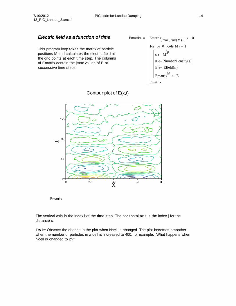
This program loop takes the matrix of particlepositions M and calculates the electric field atthe grid points at each time step. The columnsof Ematrix contain the jmax values of E atsuccessive time steps.

Contour plot of E(x,t)

Ematrix

The vertical axis is the index i of the time step. The horizontal axis is the index j for thedistance x.

Try it: Observe the change in the plot when Ncell is changed. The plot becomes smootherwhen the number of particles in a cell is increased to 400, for example. What happens whenNcell is changed to 25?



The electric field has maxima and minima at 1/4 and 3/4 of the distance across the simulationdomain. Below we find the indices j1 and j2 corresponding to these positions.

j1 floor1

4jmax

j2 floor3

4jmax

C 1

Plot of E(x,t) at the x positions where E(x,t) is greatest

0 5 10 15 200.6

0.4

0.2

0

0.2

0.4

0.6

Ematrixj1 ii

Ematrixj2 ii

Tii

Recall that we defined an initial wave amplitude: Ewave 0.5



Energy conservation as a check on accuracy in our PIC code

We will examine the "goodness" of our code by looking at energy conservation. We will findthe kinetic energy of the particles and the energy in the wave and see if their sum is constantwith time.

Kinetic Energy

Create a vector that is the sum over particles of the kinetic energy 0.5 v2 at each time step.Recall that the vector Velocities contains the velocities of the particles.

Nparticles rows Velocities( ) Nparticles 8000 Number of particles.

KinEnergyii

0.5 L

Nparticles0

Nparticles 1

k

Velocitiesk ii 2

The sum of the squares of the velocities divided by the number of PIC particles gives the meansquared velocity. The dimensionless density is unity, hence the "true" number of particles is L.The rms velocity is multiplied by L to obtain the total kinetic energy of particles.

Plot of kinetic energy of particles as a function of time

0 5 10 15 207.8

8

8.2

8.4

8.6

8.8

9

KinEnergyii

Tii

Wave energy

Recall that Ematrix has the E values at the grid points rows Ematrix( ) 81

We will integrate 0.5 E2 with distance to find the electric field energy:

WaveEnergyii

0.5 Δx

1

rows Ematrix( ) 1

k

Ematrixk ii Ematrix

k 1 ii

2

2

The above sum is the numerical equivalent of the integral of 0.5 E2 over the distance L. E isevaluated at the center of the cell by averaging the values at the adjacent grid points.



Plot of the electric field energy in the wave

0 5 10 15 200

0.2

0.4

0.6

0.8

1

WaveEnergyii

Tii

Total Energy is nearly conserved

TotEnergy WaveEnergy KinEnergy

The maximum, minimum, andstarting energies are compared.

max TotEnergy( )

TotEnergy0

1.004min TotEnergy( )

TotEnergy0

0.996

Normalized total energy as a function of time

0 5 10 15 200.98

0.99

1

1.01

1.02

TotEnergyii

TotEnergy0

0.98

1.02

Tii Tii Tii

The total energy has been divided by the initial energy to obtain a normalized value near unity.The graph will "autoscale" to make the variation look large, hence we have added points at 98%and 102% of the starting value so that the variation is shown on an appropriate scale.

Note that the error in the total energy is less than 1%, indicating that our PIC code conservesenergy (almost).



Modification of the distribution function by wave-particle interaction

To see the effect of the wave on f(v), we can plot f(v) before and after the wave is damped. The last column of the matrix Velocites contains the velocities at the last time step.

cols Velocities( ) 1 188 This is the same as the number of time steps. iters 188

These commands make a histogram of the velocities at the zeroth time step:

span max Velocities 0 min Velocities 0 span 6.045

H histogram bins Velocities 0

Histogram of f(v) before damping

4 2 0 2 40

0.1

0.2

0.3

0.4

0.5

bins H1

span Nparticles

f vplot( )

H0

vplot

bins 50These commands make a histogram of thevelocities at the last time step:

H histogram bins Velocities iters

These are the maximum and minimum values in the histogram chart:

span max Velocities iters min Velocities iters span 7.92

Histogram of f(v) after damping



4 2 0 2 40

0.1

0.2

0.3

0.4

0.5

bins H1

span Nparticles

f vplot( )

H0

vplot

Comparison of the histograms shows that there are more particles near velocity 4 after the wavehas damped as a result of the transfer of energy from the wave to the particles.

Reference :

"Plasma Physics via Computer Simulation" by C.K. Birdsall and A.B Langdon, Institute ofPhysics, Bristol and Philadelphia, 1991.



Exercises

1. Can we verify the dispersion relation for electrostatic waves?

In our dimensionless units system with the velocity scale being the square root of Te/m,

the dispersion relation is:

ω K( ) 1 3 K2

Below is an image of a plot of oscillations with L = 32 which results in a wave very near theplasma frequency.

Here is an image of a plot that shows the oscillations with L = 16.

Note that there are 8 oscillations in a time of 16 with L = 32 and 9.5 oscillations with L = 16.The observed oscillation frequency is slightly higher than the frequency from the dispersionrelation. The agreement is better if the 3 in the dispersion relation is changed to 3.3.Nevertheless, we see that the frequency is nearest the plasma frequency for long wavelengthand is higher at short wavelength.



2. Is the observed damping near the theoretical value?

The theoretical expression for Landau damping is (in our dimensionless units):

ωi 0.22 π1

K 2

3

e

1

2K2

ωi 0.089

where i is the imaginary part of the frequency. Below are images of plots of the expected

decay of the wave envelope with the electric field from the PIC code. The plots show dampingfor two values of K.

Comparison of theoretical damping and PIC code damping for two K values

The observed field of the wave has an envelope that compares well with the expected envelope.There appears to be some loss of amplitude in the first half oscillation that is not expected.



3. What if the distribution function is a top hat?

The image below is of a plot of (t) made using the top hat distribution. It shows that there is verylittle damping. Note that the number of iterations was increased so that the wave was followed formore periods.

The histogram below shows the effect of the wave on the distribution function.

Plots of the wave and particle energy show that some energy is transferred back and forthbetween the wave and the particles but there is no long term trend.



4. Can we observe echoes?

Echoes occur because the electrons oscillate in the potential wells of the waves. Thisoscillation occurs for electrons with velocities very near the wave phase velcocity. Faster orslower electrons pass over the tops of the potential hills and do not oscillate. The oscillationfrequency is determined by the amplitude of the wave, Ewave, and the wavenumber K whichtogether determine the "spring constant" of the electron oscillations. The period varies as thesquare root of Ewave. Here we compare the wave energy as a function of time for two waveamplitudes. Note that the amplitude oscillations have a shorter period for the wave of higheramplitude. The period is reduced to about 0.7 of its former value if Ewave is doubled. The effectis called an echo because the wave "reappears" after decreasing.

These plots show that the Landau damping rate should be measured for waves with smallamplitude to prevent the result from being affected by the amplitude oscillations.

particle-in-cell code for landau dampingcips.colorado.edu/mathcad/13_pic_landau_8.pdf · 7/10/2012...

Documents