parametric resonance in immersed elastic...

Parametric Resonance inImmersed Elastic Boundaries

John Stockie

Department of MathematicsSimon Fraser University

Burnaby, British Columbia, Canada

[email protected]://www.math.sfu.ca/˜stockie/

November 2, 2004

Acknowledgments

Ricardo Cortez Douglas Varela Charles PeskinTulane University CalTech Courant Institute

Natural Sciences and Engineering

Research Council of Canada

TEXpower document class: http://ls1-www.cs.uni-dortmund.de/˜lehmke/texpower/

University of Washington – Nov. 2, 2004 2

Outline

1. Review of

• “normal” resonance =⇒ external forcing• parametric resonance =⇒ internal forcing

2. Floquet stability analysis for parametrically-excited springs

3. Immersed boundary model

4. Parametric resonance in immersed boundaries

5. Numerical simulations

6. Summary and future work


1. Review of Resonance

For a damped, mass-springsystem:

mx + µx + σx = f(t)

f(t)

µ (damping)

σ (stiffness)

m(mass) (force)

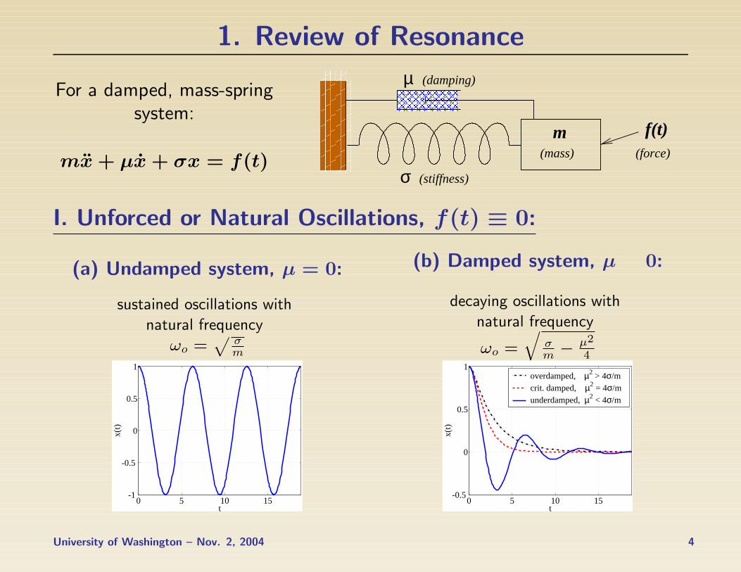
1. Review of Resonance

For a damped, mass-springsystem:

mx + µx + σx = f(t)

f(t)

µ (damping)

σ (stiffness)

m(mass) (force)

I. Unforced or Natural Oscillations, f(t) ≡ 0:

(a) Undamped system, µ = 0: (b) Damped system, µ > 0:

sustained oscillations with

natural frequency

ωo =√

σm

decaying oscillations with

natural frequency

ωo =

√σm −

µ2

4

0 5 10 15−1

−0.5

0

0.5

1

t

x(t)

Student Version of MATLAB

0 5 10 15−0.5

0

0.5

1

t

x(t)

overdamped, µ2 > 4σ/m crit. damped, µ2 = 4σ/munderdamped, µ2 < 4σ/m



II. Externally-forced Oscillations:

The system is subjected to an external periodic force(modeled as a separate term in the DE)

mx + µx + σx = Fo cos ωt

Resonance occurs when forcing is close to the natural frequency=⇒ amplitude of resulting oscillations grows when undamped (µ = 0)

(a) Undamped, non-resonant(µ = 0, ω 6= ωo):

(b) Undamped, resonant(µ = 0, ω = ωo):

persistent, mixed-frequency oscillations unstable, unbounded oscillations

0 5 10 15−6

−4

−2

0

2

4

t

x(t)


0 5 10 15−60

−40

−20

0

20

40

t

x(t)



(c) With damping (µ > 0) — “real” systems:

• oscillations are bounded, transient dies out, and forcing persists

• resonance appears as a peak in max. amplitude, only if µ2 < 12σ

2

0 5 10 15 20 25 30−4

−2

0

2

4

t

x(t)


0 1 2 3 4 50

0.05

0.1

0.15

0.2

ωres

µ2 < σ2/2

µ2 > σ2/2

Forcing frequency, ω

Am

plitu

de,

A(ω

)


Compare to the frequency–response curve for the undamped system:

0 1 2 3 4 50

0.5

1

1.5

2

Forcing frequency, ω

Am

plitu

de,

A(ω

)



III. Internal forcing:

Oscillations can also be excited via periodic variation in a system parameter:

mx + µx + σ(t)x = 0

σ(t) periodic: σ(t) = σ(t+ T ) =⇒ Hill’s equation (1886)

special case: σ(t) = σo(1 + 2ε cosωt) =⇒ Mathieu equation (1868)

Compare:• Solution can become unstable whether or not µ = 0 !

=⇒ called parametric resonance

• The system responds at frequency 12 ω [ Why? ]

• Internal forcing can also stabilize systems that are otherwiseunstable

e.g., inverted pendulum with gravitationalmodulation

ω


A Heuristic Look at Parametric ResonanceTake m = 1, µ = 0, and treat the periodic term as a forcing term:

x + ω2ox = −2εω2

o(cos ωt)x

where ω2o = σo.

First solve the homogeneous problem:

x+ ω2ox = 0 =⇒ x(t) = A cos(ωot− ϕ)

Substitute into the right hand side:

x+ ω2ox = −2Aεω2

o cosωt cos(ωot− ϕ)

= −Aεω2o

cos

[(ω + ωo)t− ϕ

]+ cos

[(ω − ωo)t− ϕ

]Resonance ensues if ω − ωo = ωo or ωo = 1

2 ω

responsefrequency = 1

2

(forcing

frequency

)University of Washington – Nov. 2, 2004 8

Examples of Parametric Resonance

• Springs or pendula with moving supports



• RLC circuits with periodically-varying inductance or capacitance




• A child pumping a swing [Curry, 1976]





• Solar surface heating generating atmospheric convection cells or patternedground formation [McKay, 1998]






• Surface waves in fluids and granular materials =⇒ Faraday instability[Faraday, 1831; Benjamin & Ursell, 1954]






• Surface waves in fluids and granular materials =⇒ Faraday instability[Faraday, 1831; Benjamin & Ursell, 1954]

• Two-fluid interfaces [Kumar & Tuckerman, 1994]

• Bubble oscillations and sonoluminescence [Brenner, Lohse & Dupont, 1995]

• Many problems in aerodynamics involving wing stability and flutter (butwing oscillations are small and have no influence on the flow)

There are many examples in fluids, but almost no analysis for fluid-structureinteraction problems.


Faraday Waves

ω

F (t) = mg(1 + 2ε cosωt)

Faraday (1831) observed that:

• regular, symmetric patterns arise on the surface

• waves oscillate with twice the period of the parametric forcing

Stripes (1-fold symmetry) Squares (2-fold symmetry) Hexagons (3-fold symmetry)

Source: Dept. of Physics, University of Torontohttp://mobydick.physics.utoronto.ca/faraday.html


http://mobydick.physics.utoronto.ca/faraday.html

Some Results from Floquet Theory

For homogeneous, periodic, linear systems:

x = A(t) · x, where A(t) ∈ Rn×n, x(t) ∈ Rn (*)

and A(t+ T ) = A(t), for some T > 0.

Floquet Theorem (Bloch Theorem in solid state physics):

Every fundamental matrix solution X(t) of (*) has the form:

X(t) = eBt · P (t)

where P (t+ T ) = P (t) and B = constant.

Corollary: Any solution of(*) is a linear combination offunctions of the form: eγt · p(t)

1

HHHH

HHj

“Floquet” or

characteristic exponent, γ ∈ C

a polynomial with

T-periodic coefficients


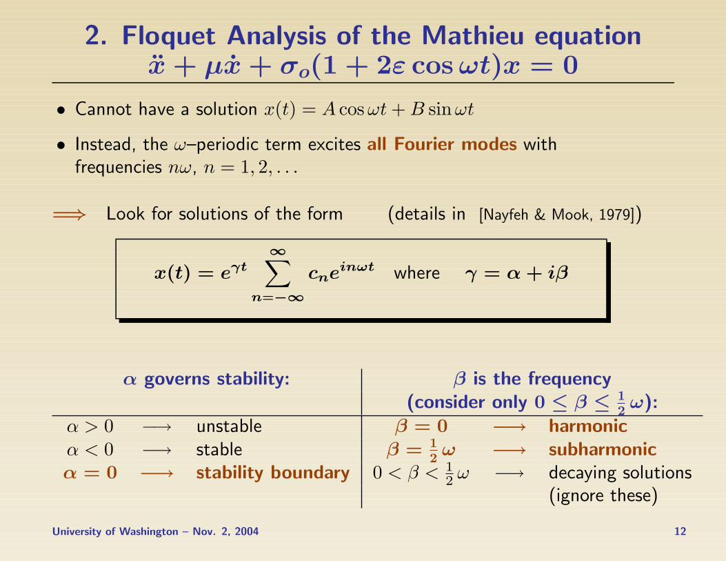
2. Floquet Analysis of the Mathieu equationx + µx + σo(1 + 2ε cos ωt)x = 0

• Cannot have a solution x(t) = A cosωt+B sinωt

• Instead, the ω–periodic term excites all Fourier modes withfrequencies nω, n = 1, 2, . . .

=⇒ Look for solutions of the form (details in [Nayfeh & Mook, 1979])

x(t) = eγt∞∑

n=−∞cneinωt where γ = α + iβ

α governs stability: β is the frequency(consider only 0 ≤ β ≤ 1

2 ω):α > 0 −→ unstable β = 0 −→ harmonicα < 0 −→ stable β = 1

2 ω −→ subharmonicα = 0 −→ stability boundary 0 < β < 1

2 ω −→ decaying solutions(ignore these)


Substitute

x(t) =∞∑

n=−∞cne

(γ+inω)t into x+ µx+ σo(1 + 2ε cosωt)x = 0

Interested only in the stability boundary where α = 0 (i.e., γ = 0 + iβ):

∞∑n=−∞

cnei(β+nω)t

−(β + nω)2+ iµ(β + nω) + σo

1 + ε(eiωt

+ e−iωt

)︸︷︷︸

shifts n by ±1

= 0

Substitute

x(t) =∞∑

n=−∞cne

(γ+inω)t into x+ µx+ σo(1 + 2ε cosωt)x = 0

Interested only in the stability boundary where α = 0 (i.e., γ = 0 + iβ):

∞∑n=−∞

cnei(β+nω)t

−(β + nω)2+ iµ(β + nω) + σo

1 + ε(eiωt

+ e−iωt

)︸︷︷︸

shifts n by ±1

= 0

=⇒ [σo − (β + nω)2 + iµ(β + nω)]cn + εσo(cn−1 + cn+1) = 0 (**)

Aim: To find real values of ε:

• split (**) into real and imaginary parts,

• let cn = crn + icin, and . . .


define ~c = [. . . , crn−1, cin−1, c

rn, c

in, . . . ]

T so (**) can be written in matrix form:. . .

0 0 An −Bn 0 00 0 Bn An 0 0

. . .

~c+ εσo

. . .

1 0 0 0 1 00 1 0 0 0 1

. . .

~c = 0


define ~c = [. . . , crn−1, cin−1, c

rn, c

in, . . . ]

T so (**) can be written in matrix form:. . .

0 0 An −Bn 0 00 0 Bn An 0 0

. . .

︸︷︷︸

D

~c+ εσo

. . .

1 0 0 0 1 00 1 0 0 0 1

. . .

︸︷︷︸

E

~c = 0

where An = σo − (β + nω)2 and Bn = µ(β + nω).

More compactly:

(−σoD−1E)~c =(

1

ε

)~c,

An infinite-dimensional eigenvalue problem witheigenvalues 1

ε, and

eigenvectors ~c.


Details:

• Cut off at a finite N , i.e.,∞∑−∞

−→N∑−N

(since cn → 0 as |n| → ∞)

• Apply “reality conditions”:

c−n = c∗n, if β = 0 (harmonic) c−n = c∗n−1, if β = 1

2 ω (subharmonic)

to eliminate all cn with n < 0 =⇒ a (2N + 2)× (2N + 2) linear system

• Parameter values:µ, ω: given

α = 0: for stability boundariesβ = 0, 1

2 ω: for harmonic/subharmonic casesN = 15: chosen so that |cn| 1 for all |n| > N

ε: comes from solving the eigenvalue problemσo: is a free parameter

Basic Idea: for each σo, we obtain 2N + 2 values of ε. . . pick the positive, real ones.


Stability of the Mathieu equationx + µx + σo(1 + 2ε cos ωt)x = 0

Ince-Strutt Diagram (ω = 2, µ = 0):

5 10 15 20 25 300

5

10

15

20

σ0

ε σ 0

ε=1/2

ω=2, µ=0

1 4 9 16 25

unst

able

stabl

e

stabl

eun

stab

le

... = harmonic (β = 0)

... = subharmonic (β = 12 ω)

• Eigenvalues divide the planeinto stable and unstable regions=⇒ tongues of instability

• ε ≤ 12 are “physical” eigenvalues

• ε = 0 gives natural modes,σo = n2



5 10 15 20 25 300

5

10

15

20

σo

ε σ o

ε=1/2

ω=2, µ=0.0, 0.6

ε=1/2

Increase damping further to µ = 0.6=⇒ no more physical instabilities



5 10 15 20 25 300

5

10

15

20

σo

ε σ o

ε=1/2

ω=2, µ=0.0, 0.6, 2.0

ε=1/2 ε=1/2

Increase damping to µ = 2.0

[ movie ]

Note:

• even small perturbations (ε ≈ 0) can lead to instability if µ is small enough

• damping has a stabilizing influence=⇒ the ω = 2 problem is stable if µ ' 0.6


3. Immersed BoundariesMove on to fluid-structure interaction problems ...

“Life is . . . fiber-reinforced fluid.”

– C. S. Peskin (1999)

3. Immersed BoundariesMove on to fluid-structure interaction problems ...

“Life is . . . fiber-reinforced fluid.”

– C. S. Peskin (1999)

Biological fibers, and surfaces constructed of fibers, immersed in fluid:

• heart and blood vessels

• worms and leeches

• flagellae and cilia

• plant cells (esp. wood)

• microtubules and actin filaments

• suspensions of proteins, DNA, polymers, etc.


Example: The Heart

Peskin and McQueen (2000): Simulations of the beating heart

Source: http://www.psc.edu/science/Peskin/Peskin.html

[ movie0 ] [ movie1 ] [ movie2 ] [ movie3 ]


http://www.psc.edu/science/Peskin/Peskin.html

Fiber Architecture of theHeart Muscle Wall

[Dissected pig heart: Carolyn Thomas, 1957]


The Immersed Boundary Model

Simplifying assumptions:

• 2D fluid with a single, impermeable, elastic membrane (or fiber)

• fiber has zero volume and mass, and is neutrally buoyant

• fluid lies both inside and outside the fiber

• domain is periodic

• in 3D, surfaces are built from an interwoven mesh of fibers

The Immersed Boundary Model

Simplifying assumptions:

• 2D fluid with a single, impermeable, elastic membrane (or fiber)

• fiber has zero volume and mass, and is neutrally buoyant

• fluid lies both inside and outside the fiber

• domain is periodic

• in 3D, surfaces are built from an interwoven mesh of fibers

Ω Γ

Ω = fluid domainp(~x, t) = fluid pressure~u(~x, t) = fluid velocity

Γ = fibers = arclength parameter~X(s, t) = fiber position~U(s, t) = fiber velocity~F (s, t) = fiber force density = σ∂2

s~X (“springs”)


Dynamic interaction between fluid and fiber:

• the fiber exerts a singular force on adjacent fluid particles:

ρ (∂t~u+ ~u · ∇~u) = µ∆~u−∇p +∫

Γ

~F (s, t) δ(~x− ~X(s, t)) ds

∇ · ~u = 0

(Navier-Stokes equations with a singular force)

Dynamic interaction between fluid and fiber:

• the fiber exerts a singular force on adjacent fluid particles:

ρ (∂t~u+ ~u · ∇~u) = µ∆~u−∇p +∫

Γ

~F (s, t) δ(~x− ~X(s, t)) ds

∇ · ~u = 0

(Navier-Stokes equations with a singular force)

• fiber moves at the fluid velocity – the no slip condition:

∂t ~X = ~u( ~X(s, t), t) =∫

Ω

~u(~x, t) δ(~x− ~X(s, t)) d~x

=⇒ interactions are mediated by delta functions!

An alternate formulation eliminates delta functions in favour ofjump conditions =⇒ immersed interface method [Leveque & Li, 1994]


Previous Work1. A linear stability analysis for unforced fibers, initially deformed and then

released [JS & Wetton, 1995]:

• unconditionally stable (α > 0)

• dependence of solution on parameters (Re, σo) is non-trivial





2. A nonlinear stability analysis for a passive circular membrane in an inviscidfluid [Cortez & Varela, 1997]






Question:What happens when a fiber is pulsed periodically

(like a heart muscle fiber)?






Question:What happens when a fiber is pulsed periodically

(like a heart muscle fiber)?

3. A related problem [Wang, 2003]:

• Floquet-type analysis for buckling instabilities in a headbox, assumingsmall deformations

• flow oscillations drive the structure BUT the structure has no effect onthe fluid


4. Stability Analysis for Immersed Boundaries

Investigate the stability of a perturbedcircular fiber with periodically-varyingstiffness

σ(t) = σo(1 + 2ε cosωt)(X ,X )r θ

θ

r=1

r

4. Stability Analysis for Immersed Boundaries

Investigate the stability of a perturbedcircular fiber with periodically-varyingstiffness

σ(t) = σo(1 + 2ε cosωt)(X ,X )r θ

θ

r=1

r

Simplifications:

• Assume small perturbations about r = 1

• Linearize the Navier–Stokes equations =⇒ Stokes’ equations

• Convert to stream function & vorticity: u, v −→ ψ, ξ

• Integrate the Navier-Stokes equations across the fiber=⇒ eliminates δ–functions in favour of jump conditions


The Stream Function–Vorticity FormulationInner (r < 1) and outer (r > 1) solutions both obey:

∆ψ = −ξ

∂tξ =µ

ρ∆ξ

Immersed boundary equation:

∂t ~X = (∂θψ,−∂rψ)|r=1

Jump conditions, with [[·]] .= (·)|r=1+ − (·)|r=1−:

[[ψ]] = 0, [[ξ]] =p2σoiωµ

(ψ(1)− ∂rψ(1))

[[∂rψ]] = 0, [[∂rξ]] =p2(p2 − 1)σo

iωµψ(1)

Boundary conditions:

ψ and ξ bounded as r →∞periodic matching at θ = 0 and 2π


Floquet–type solutions:

For ξ (and ψ):

ξ(r, θ, t) = eipθ︸︷︷︸periodicin θ

∞∑n=−∞

ξn(r) e(γ+inω)t︸︷︷︸same as before

For Xr (and Xθ):

Xr(θ, t) = eipθ∞∑

n=−∞Xrn e

(γ+inω)t

Substitute and obtain a Bessel equation for ξn:

z2ξ′′n(z) + zξ′n(z) + (z2 − p2)ξn(z) = 0

where z.= −(Ωn r)2 and Ωn

.=

√ρ(γ + inω)

µ


Solution: can be written in terms of Bessel functions, Jp and Hp:

ξn(r) =

anHp(iΩnr), if r > 1 (outer)

bnJp(iΩnr), if r < 1 (inner)

and ψn(r) =

combinations of Jp, Hp, r

−p and rp

. . .

Applying jump conditions yields the two equations:

0 = i

µ2

σoΩ

3n

[Hp(iΩn)

Hp−1(iΩn)−

Jp(iΩn)

Jp+1(iΩn)

]+ ip

Xrn

+

µ2

σoΩ

3n

[Hp(iΩn)

Hp−1(iΩn)+

Jp(iΩn)

Jp+1(iΩn)

]− ip

2

Xθn

+ iεp(Xrn−1 −X

rn+1

)− εp

2(Xθn−1 −X

θn+1

)0 = i

µ2

σoΩ

4n

[2−

Hp+1(iΩn)

Hp−1(iΩn)−Jp−1(iΩn)

Jp+1(iΩn)

]+ 2p(p

2 − 1)

Xrn

+µ2

σoΩ

4n

[Hp+1(iΩn)

Hp−1(iΩn)−Jp−1(iΩn)

Jp+1(iΩn)

]Xθn + 2εp(p

2 − 1)(Xrn−1 −X

rn+1

)

View as a linear system in the unknowns[Re(Xr

n), Im(Xrn), Re(X

θn), Im(Xθ

n)]!


After some messy algebra, obtain another eigenvalue problem

(−D−1E)~c =(

1ε

)~c

where D and E are infinite, real matrices consisting of 4× 4 blocks.

Basic Idea (same as for the Mathieu equation):

• Cut off at finite N

• Look for stability boundaries, γ = 0 and 12iβ

• Parameter space is now the p–ε plane (σo is scaled out)

• Results are reported in terms of the nondimensional parameters

κ =σo

ρω2oR2

and ν =µ

ρωoR2

Question:Are there regions of instability for physically-reasonable

parameter values?


Stability Diagrams for the Forced Problem

Case I: Case II:κ = 0.04, ν = 0.00056 κ = 0.4, ν = 0.001

p = 4 mode is unstable p = 2 mode is unstable

0 2 4 6 8 100

0.5

1

1.5

2

2.5

3

wave number, p

ampl

itude

, ε

κ = 0.04 ν = 0.00056

HH

H

HH

S

S

S

S


0 1 2 3 40

0.5

1

1.5

2

2.5

3

wave number, p

ampl

itude

, ε

κ = 0.4 ν = 0.001 nmax = 40

H

H

H

S

S

S

[ κ ] [ ν ]


Compile the minimum ε over a range of κ and ν:

10−2

10−1

10−4

10−3

10−2

10−1

0.3

0.5

1

2

5

stiffness, κ

visc

osit

y, ν

Contours of eigenvalues, ε

ε=1/2

Stable

Unstable

A straight–line fit to the ε = 12 stability boundary yields

ν = 0.0389 · κ0.626

(. . . interesting . . . can this be explained?)

Next, compare to both computations and previous analyses . . .


Natural modes – unforced problem

• consider a fiber with no forcing, ε = 0

• take the n = 0 mode

• the eigenvalue equations reduce to a single dispersion relation

The decay rate and frequency can be compared to direct numerical simulations

10−6

10−4

10−2

0

0.5

1

1.5

2

2.5

3

ν2/κ

Decay rate

−α/

κ1/2

p = 2p = 3p = 4


10−6

10−4

10−2

0

1

2

3

4

5

6

ν2/κ

Frequency

β/κ1/

2ω

N(2)

ωN

(3)

ωN

(4) p = 2p = 3p = 4


This represents an exact (asymptotic) solution that can be used tovalidate 2D computations!!!


Natural modes – small ν limit

In the limit as ν → 0, we obtain

Decay rate: α = 0

Frequency: β = ωN√κ where ωN(p) = p

√(p2 − 1)/2.

=⇒ matches the inviscid analysis of [Cortez & Varela, 1997]

Natural modes – small ν limit

In the limit as ν → 0, we obtain

Decay rate: α = 0

Frequency: β = ωN√κ where ωN(p) = p

√(p2 − 1)/2.

=⇒ matches the inviscid analysis of [Cortez & Varela, 1997]

Asymptotic expansion of the dispersion relation in ν yields:

Decay rate: α ∼ − p

2√

2ω

1/2N κ1/4

√ν

Frequency: β ∼ ωN√κ− p

2√

2ω

3/4N κ1/4

√ν

=⇒ matches the viscous analysis of [JS & Wetton, 1995]


5. Numerical Simulations

“Usual” implementation of the immersed boundary method [Peskin, 1977]

• second order centered differences in space

• split step projection method

• delta function approximation reduces spatial accuracy to first order

• first order and explicit in time

Notice: small discrepancies between analysis and numerics owing to

• artificial dissipation from the numerical scheme

• numerical errors from the first order time–stepping

We have also run fully second-order simulations using the blob projectionmethod [Cortez & Minion, 2000]


Unforced fiber simulations

Fiber is initially perturbed with a p–mode of magnitude 0.05

Case I: κ = 0.04, ν = 0.00056, p = 4

Initial Amplitude of p = 4 mode

−1.5 −1 −0.5 0 0.5 1 1.5−1.5

−1

−0.5

0

0.5

1

1.5

x/R

y/R


0 50 100 150−0.05

0

0.05

t

Am

plitu

de


[ movie ]


Forced fiber simulations

Fiber is initialized and forced with the same resonant p–mode

Case I: κ = 0.04, ν = 0.00056, p = 4

Amplitude of p = 4 mode Vary parameters

0 50 100 150−0.2

−0.1

0

0.1

0.2

0.3

t

Am

plitu

de


0.5 1 1.5 2 2.5 3 3.5 4

x 10−3

0

0.05

0.1

0.15

0.2

0.25

0.3

viscosity, νM

ax. a

mpl

itude


[ movie ]0.03 0.04 0.05 0.06 0.07 0.080

0.1

0.2

0.3

0.4

0.5

stiffness, κ

Max

. am

plitu

de



Case II: κ = 0.5, ν = 0.001, p = 2

Amplitude of p = 2 mode Vary Parameters

0 50 100 150 200−0.3

−0.2

−0.1

0

0.1

0.2

0.3

0.4

t

Am

plitu

de


2 4 6 8 10 12 14 16

x 10−3

0

0.1

0.2

0.3

0.4

0.5

viscosity, νM

ax. a

mpl

itude


[ movie ]0.4 0.45 0.5 0.55 0.6 0.650

0.1

0.2

0.3

0.4

0.5

stiffness, κ

Max

. am

plitu

de

Student Version of MATLABUniversity of Washington – Nov. 2, 2004 35

Energy Transfer from Resonant Modes

Because of numerical errors, the fiber motion is not a pure p–mode

• most of the energy remains in the resonant mode

• Even p: small perturbations appear in all np–modes

• Odd p: asymmetry leads to a small “drift” or p = 1 mode

=⇒ all p-modes are excited! [ sin(p± q) = sin p cos q ± cos p sin q ]

Case I, initialized with p = 3 mode Energy transfers to the resonant p = 4 mode

−1.5 −1 −0.5 0 0.5 1 1.5−1.5

−1

−0.5

0

0.5

1

1.5

x/R

y/R

0 20 40 60 80−0.15

−0.1

−0.05

0

0.05

0.1

t

Am

plitu

de

Amplitude of p−modes

p=3p=4

[ movie ]


Application to Atrial Fibrillation

Parameter Units Human heart 3D numerics

normal fibrillated (Peskin-McQueen)

ρ g/cm3 1.0 1.0 1.0

µ g/cm s 0.04 0.04 1.0

σo g/cm s2 1000? 1000? 1000?

ωo rad/s (bt/min) 6.3 (60) 18.3 (170) 7.3 (70)

R cm 3.2 3.2 3.2

κ = σoρω2R2 – 2.47 0.29 1.83

ν = µ

ρωR2 – 0.00062 0.00021 0.013

10−2 10−1 100

10−4

10−3

10−2

10−1

Fib

Norm

Num 0.3

0.5

1

2

5

stiffness, κ

visc

osity

, ν


ε=1/2

Unstable

Stable


• Most studies of atrial fibrillation point to electrophysiological causes.

• Our analysis suggests a possible fluid–mechanical contribution to fibrillationthrough feedback into propagation of electrical signals (?)

However, we still don’t expect instabilities to develop in normal hearts!Possible explanations:

• nonlinearities tend to stabilize:

the fiber, introducing a rest length Ro 6= 0 the fluid, moving to higher Reynolds number

• 3D effects are missing:

added stability of an interwoven fiber mesh thickness of the heart wall a heart beat is actually a spiral wave, not a homogeneous pulse


Application to Cochlear MechanicsThe cochlea is a spiral-wound, fluid-filled tube, which propagates waves alongthe basilar membrane (BM):

Recent research aims to explain the amazing sensitivity of the BM to soundwaves in the presence of large viscous damping:

• (experiments) outer hair cells change length in response to shearing

• modulates the stiffness of the BM

• introduces a mechanical feedback that amplifies BM motions


Cochlea and basilar membrane

Outer hair cell Organ of Corti


Parameter Units Cochlea

ρ g/cm3 1.0

µ g/cm s 0.01

σo g/cm s2 1000

ω rad/s 1000+

R cm 0.2

κ = σoρω2R2 – 0.025

ν = µ

ρωR2 – 0.00025 10−2 10−1 100

10−4

10−3

10−2

10−1

Fib

Norm

Num

BM 0.3

0.5

1

25

stiffness, κ

visc

osity

, ν


• Current models of cochlear mechanics focus on mechanical resonance[Martin et al., 2000], [Nobili et al., 1998]

• Our analysis suggests that fluid-mechanical feedback may also play asignificant role

• BUT we’re still missing 3D effects, nonlinearities in BM stiffness, andcoupling to mechanical effects


6. Summary

• performed a Floquet analysis of a parametrically-forced immersed boundary

• derived an analytical (leading-order, asymptotic) solution which can beused to validate 2D numerical simulations – the first such exact solution!

• matched results with previous analyses of the unforced problem in thesmall-viscosity limit

• identified parameter ranges in which forced fiber dynamics are unstable

Warning:(for people simulating active, biological interfaces)

watch out for parametric resonances, which can easilybe mistaken for numerical instabilities!

• suggested possible parametric resonance in biological systems such as thehuman heart and cochlea


Future Work

• a 3D numerical study of forced immersed boundaries

• spatially-varing stiffness, σ(θ, t) =⇒ simulates spiral wave propagation

• extend to fiber spring force with non-zero resting length, Ro:

~f(s, t) = σ ∂2s~X =⇒ ~f(s, t) = σ ∂s

[∂s ~X

(1−Ro

/∣∣∣∂s ~X∣∣∣)]

• “step–function” forcing

σ

t is better than

σ

t

• optimal control of forced immersed boundaries, with application topacemaker design

=⇒ external forcing f(t) = A cos Ωt, with Ω a control parameter


References

[1] T. B. Benjamin and F. Ursell. The stability of the plane free surface of a liquid in vertical periodic motion.Proc. Roy. Soc. Lond. A, 225(1163):505–515, 1954.

[2] R. P. Beyer, Jr. A computational model of the cochlea using the immersed boundary method. J. Comput.Phys., 98:145–162, 1992.

[3] M. P. Brenner, D. Lohse, and T. F. Dupont. Bubble shape oscillations and the onset of sonoluminescence.Phys. Rev. Lett., 75:954–957, 1995.

[4] R. Cortez and M. Minion. The blob projection method for immersed boundary problems. J. Comput. Phys.,161(2):428–453, 2000.

[5] R. Cortez and D. A. Varela. The dynamics of an elastic membrane using the impulse method. J. Comput.Phys., 138:224–247, 1997.

[6] S. M. Curry. How children swing. Amer. J. Phys., 44(10):924–926, 1976.

[7] M. Faraday. On a peculiar class of acoustical figures; and on certain forms assumed by groups of particlesupon vibrating elastic surfaces. Phil. Trans. Roy. Soc., 121:299–340, 1831.

[8] G. Floquet. Sur les equations differentielles lineaires a coefficients periodiques. Ann. Sci. Ecole Norm. Sup.,12(2):47–88, 1883.

[9] K. Kumar and L. S. Tuckerman. Parametric instability of the interface between two fluids. J. Fluid Mech.,279:49–68, 1994.

[10] P. Martin, A. D. Mehta, and A. J. Hudspeth. Negative hair-bundle stiffness betrays a mechanism formechanical amplification by the hair cell. Proc. Natl. Acad. Sci. USA, 97(22):12026–12031, 2000.

[11] G. McKay. Onset of double-diffusive convection in a saturated porous layer with time-periodic surfaceheating. Continuum Mech. Thermodyn., 10:241–251, 1998.

[12] D. M. McQueen and C. S. Peskin. A three-dimensional computer model of the human heart for studyingcardiac fluid dynamics. Computer Graphics, 34(1):56–60, 2000.

[13] R. Nobili, F. Mammano, and J. Ashmore. How well do we understand the cochlea? Trends Neurosci.,21:159–167, 1998.


[14] C. S. Peskin. Numerical analysis of blood flow in the heart. J. Comput. Phys., 25:220–252, 1977.

[15] J. M. Stockie and B. T. R. Wetton. Stability analysis for the immersed fiber problem. SIAM J. Appl.Math., 55(6):1577–1591, 1995.

[16] X. Wang. Instability analysis of some fluid-structure interaction problems. Comput. Fluids, 32:121–138,2003.


parametric resonance in immersed elastic...

Documents