parameter synthesis in dynamical systems by model checking

Parameter synthesis in dynamical systems bymodel checking

David Safranek

with Nikola Benes, Lubos Brim, Martin Demko, Samuel Pastva

keynote talkSynCoP + PV 2017

Masaryk UniversityCzech Republic

SynCoP + PV 2017, ETAPS, Uppsala, 22.4.2017 1/52

Outline

1 Motivation

2 Parameter Synthesis by Coloured Model Checking

3 Discrete Bifurcation Analysis

4 Case StudiesCase Study using Parameter SynthesisCase Study using Discrete Bifurcation Analysis

5 Discussion


Outline

1 Motivation




5 Discussion


Motivation: Systems View of Processes Driving the CellTo Mechanistically Understand Natural/Physical Systems

nutrients enzymes

metabolic products

signals

proteins

regulatory elements

METABOLISM PROTEOSYNTHESIS


Motivation: Models of Complex Dynamical SystemsUnderstanding Role of Parameters

deterministic models of dynamical systems:

x = f (x(t), p)

f ... phase space (vector field), f : Rn × Rm → Rn

x ... state vector (Rn)

p ... parameter vector (Rm)

0 0,8 1,6 2,4 3,2 4 4,8 5,6 6,4 7,2 8 8,8 9,6 10,4 11,2 12 12,8 13,6 14,4 15,2 16 16,8 17,6 18,4 19,2

0,8

1,6

2,4

3,2

4

4,8

5,6

6,4

7,2

8

8,8

9,6

10,4

11,2

12

12,8

Insert text here

pRB

E2F1

0 0,8 1,6 2,4 3,2 4 4,8 5,6 6,4 7,2 8 8,8 9,6 10,4 11,2 12 12,8 13,6 14,4 15,2 16 16,8 17,6 18,4 19,2

0,8

1,6

2,4

3,2

4

4,8

5,6

6,4

7,2

8

8,8

9,6

10,4

11,2

12

12,8

Insert text here

pRB

E2F1

p = 0.006 p = 0.012


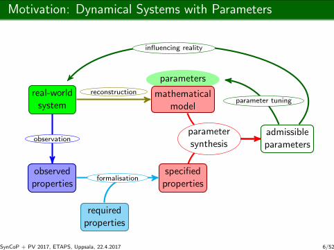
Motivation: Dynamical Systems with Parameters

parameters

real-worldsystem

mathematicalmodel

observedproperties

specifiedproperties

requiredproperties

admissibleparameters

influencing reality

observation

reconstruction

formalisation

parameter tuning

parametersynthesis


Model-Based Dynamical Systems AnalysisEmploying Constraints on Systems Dynamics

(bio)physics: often use parameterised non-linear ODEs,supplied with local methods (e.g., simulation)

biology: observations in the form of time-series data

literature provides further constraints on systems dynamics

computer science: turn all known facts into formalspecification and find admissible model parameters

a suitable formal language is provided by temporal logics

if the model is given as a state-transition system we canemploy model checking⇒ exhaustive – global view wrt parameters and initialconditions, different than simulation


Outline

1 Motivation




5 Discussion


Problem FormulationParameter Synthesis for Dynamical Systems

parameter constraints

behavior constraints

p |=ΦI ∧M

(p) |=ϕ

parametrised modelM(p)

restrictp

restrictM

ϕ

ΦI

Parameter Synthesis Problem

Assume P is the admissible parameter space. Given a behaviourconstraint ϕ, parameter constraint ΦI , and a parameterisedmodel M, find the maximal set P ⊆ P of parameterisationssuch that p |= ΦI and M(p) |= ϕ for all p ∈ P.


Considered Parameterised Models of Dynamical Systems

a b

c

dynamical systems as regulatory networks

discrete models (e.g., Boolean networks)

parameters determine the logic of interactionsdeterministic (synchronous) vs. non-deterministic(asynchronous)finite-state, finite parameters, parameter explosion dominatesTCCB 2010, CMSB 2012, SASB 2016Henzinger et al. TACAS 2015; Ballarini et al. 2016

non-linear ODE models

continuous parameters determine the vector fieldundecidablesemi-decidable by employing approximations/abstractions

piece-wise affine and piece-wise multi-affineoverapproximation by (parametrised) finite automatastate explosion and parameter explosion


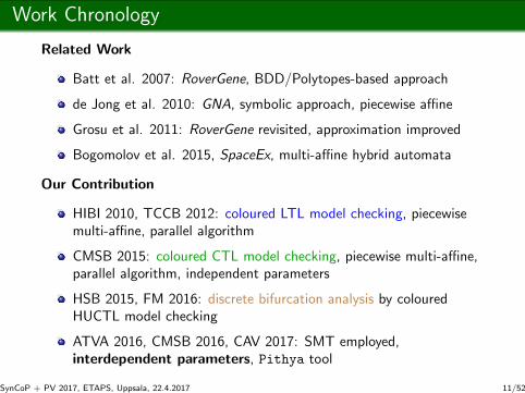
Work Chronology

Related Work

Batt et al. 2007: RoverGene, BDD/Polytopes-based approach

de Jong et al. 2010: GNA, symbolic approach, piecewise affine

Grosu et al. 2011: RoverGene revisited, approximation improved

Bogomolov et al. 2015, SpaceEx, multi-affine hybrid automata

Our Contribution

HIBI 2010, TCCB 2012: coloured LTL model checking, piecewisemulti-affine, parallel algorithm

CMSB 2015: coloured CTL model checking, piecewise multi-affine,parallel algorithm, independent parameters

HSB 2015, FM 2016: discrete bifurcation analysis by colouredHUCTL model checking

ATVA 2016, CMSB 2016, CAV 2017: SMT employed,interdependent parameters, Pithya tool


Workflow

behaviourconstraints

parameterconstraints

ODE model

PWMA model

parameterisedKripke structure

temporal formulae

valid parametervaluations

ColouredModel

Checking

formalisation approximation

abstraction


Step 1: ApproximationDiscretisable Continuous (ODE) Models

(bio)physical mechanisms modeled by sigmoidal kinetics (e.g.,signalling pathways, gene regulatory circuits, ...)optimal approximation of sigmoid functions by piece-wiseaffine functions (ramps) [Grosu et al. CAV 2011]

model abstraction kinetics

piece-wise multi-affinetransient over-approximatedsteady state over-approximated

sigmoidal kineticsmass action

piece-wise affinetransient over-approximatedsteady state exact

first-order sigmoidalkineticsSynCoP + PV 2017, ETAPS, Uppsala, 22.4.2017 13/52

Step 2: Rectangular Abstraction

approach originates in [Batt, Belta, Habets, van Schuppen 2006]

continuous phase-space is partitioned into (hypher)rectangles

no diagonal transitions, overapproximation

self-transitions, in PWMA only necessary condition for exiting abox in finite time =⇒ overapproximation

A

B


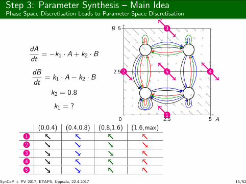
Step 3: Parameter Synthesis – Main IdeaPhase Space Discretisation Leads to Parameter Space Discretisation

dA

dt= −k1 · A + k2 · B

dB

dt= k1 · A− k2 · B

k2 = 0.8

k1 = 0.6

B

A0 2.5 5

2.5

5

(0,0.4) (0.4,0.8) (0.8,1.6) (1.6,max)1

2

3

4

5

−2.5 · k1 > 0

−2.5·k1+2.5·k2 > 0



dA

dt= −k1 · A + k2 · B

dB

dt= k1 · A− k2 · B

k2 = 0.8

k1 = 0.6

B

A0 2.5 5

2.5

5

1

2

3

45

(0,0.4) (0.4,0.8) (0.8,1.6) (1.6,max)1

2

3

4

5

−2.5 · k1 > 0

−2.5·k1+2.5·k2 > 0



dA

dt= −k1 · A + k2 · B

dB

dt= k1 · A− k2 · B

k2 = 0.8

k1 = ?

B

A0 2.5 5

2.5

5

1

2

3

45

(0,0.4) (0.4,0.8) (0.8,1.6) (1.6,max)1

2

3

4

5

−2.5 · k1 > 0

−2.5·k1+2.5·k2 > 0



dA

dt= −k1 · A + k2 · B

dB

dt= k1 · A− k2 · B

k2 = 0.8

k1 = ?

B

A0 2.5 5

2.5

5

1

2

3

45

Φstate00→state10 := −2.5 · k1 > 0 ∨ −2.5 · k1 + 2.5 · k2 > 0

The transition exists if and only if the formula is satisfiable.Local parameter constraints are predicates over reals.


Step 3: Parameter Synthesis – Main IdeaLiveness

necessary condition for escaping a state (rectangle) s in finitetime is

0 /∈ hull{f (v , p) | v ∈ vertices(s)}for all p ∈ P not satisfying the necessary condition above aself-transition is added to s:

Φs,s := ∃c1, . . . , ck :

(k∧

i=1

ci ≥ 0

)∧(

k∑i=1

ci = 1

)∧(

k∑i=1

ci · f (vi , p) = 0

)

quantifier-free formulae giving coarser overapproximation ofself-transitions can be used alternatively


WorkflowParameterised Kripke Structures and Model Checking

behaviourconstraints

parameterconstraints

parameterisedKripke structure

temporal formulae

valid parametervaluations

ColouredModel

Checking

formalisation


Parameterised Kripke StructuresState Transition Systems with Parameters

Transitions with Parameters (coloured transitions)

••

••••

••

••

•••• ••

••

•••

•••

••

••

••••

each parameter valuation represents one Kripke structure

shared state space, different transition space

symbolic representation of parameters

symbolic PKS: every transition is associated with a formula


Parameterised Kripke StructuresState Transition Systems with Parameters

Transitions with Parameters (coloured transitions)

••

••••

••

••

•••• ••••

•••

•••

••

••

••••

each parameter valuation represents one Kripke structure

shared state space, different transition space

symbolic representation of parameters

symbolic PKS: every transition is associated with a formula


Parameter Synthesis by Coloured Model Checking

LT

L o

r (A

)CT

L s

pe

cif

ica

tio

n

the specification is guaranteed(some might be missing)

the specification might be violated

parameter intervals where

[A]

[B]

5

0 2.5 5

2.5

[A][A]

parameterized Kripke structure of the model

CMC

YES NO

parameter intervals where

identify states and colors for which the property does/doesn’t hold


Parameter Synthesis by Coloured Model CheckingSome Observations

exloiting experiences with enumerative MC

many parameter values typically shared on a transition

coloured MC is an effective heuristics wrt naıve approach

parallel automata-based LTL MC [BioDiVinE – TCBB 2010]

LTL nicely preserved by the abstractionsabstractions are non-deterministicneed to analyse decision states (neighbourhood aroundunstable equillibria)we went more to monitoring/robustness analysis STL, STL*(extending work of Donze et al.)

towards coloured CTL model checking [Pithya – CAV 2017]


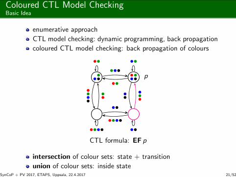
Coloured CTL Model CheckingBasic Idea

enumerative approach

CTL model checking: dynamic programming, back propagation

coloured CTL model checking: back propagation of colours

p

••

••••

••

••

•••• ••

••

••

•••

•••

•••

•••

••

••

••

••••

•••••••

•••••

CTL formula: EF p

intersection of colour sets: state + transition

union of colour sets: inside stateSynCoP + PV 2017, ETAPS, Uppsala, 22.4.2017 21/52





p

••

••••

••

••

•••• ••

••

••

•••

•••

•••

•••

••

••

••

••••

••••

•••

•••••

CTL formula: EF p







p

••

••••

••

••

•••• ••

••

••

•••

•••

•••

•••

••

••

••

••••

•••••••

•••••

CTL formula: EF p







p

••

••••

••

••

•••• ••

••

••

•••

•••

•••

•••

••

••

••

••••

•••••••

•••

••

CTL formula: EF p







p

••

••••

••

••

••••

••

••••

•••

•••

•••

•••

••

••

••

••••

•••••••

•••

••

CTL formula: EF p







p

••

••••

••

••

••••

••

••••

•••

•••

•••

•••

••

••

••

••••

•••••••

••••

•

CTL formula: EF p







p

••

••••

••

••

•••• ••

••

••

•••

•••

•••

•••

••

••

••

••••

•••••••

••••

•

CTL formula: EF p







p

••

••••

••

••

•••• ••

••

••

•••

•••

•••

•••

••

••

••

••••

•••••••

•••••

CTL formula: EF p



Parameter Synthesis by Coloured CTL Model CheckingFormal Definition

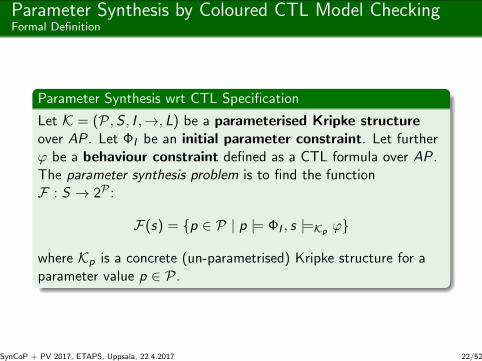
Parameter Synthesis wrt CTL Specification

Let K = (P, S , I ,→, L) be a parameterised Kripke structureover AP. Let ΦI be an initial parameter constraint. Let furtherϕ be a behaviour constraint defined as a CTL formula over AP.The parameter synthesis problem is to find the functionF : S → 2P :

F(s) = {p ∈ P | p |= ΦI , s |=Kp ϕ}

where Kp is a concrete (un-parametrised) Kripke structure for aparameter value p ∈ P.


Symbolic Representation of ParametersUsing SMT to Deal With Parameter Sets

Encoding

every set of parameters (on transitions, inside states)represented by a formula with free variables:satisfying assignments are set elements

union is disjunction, intersection is conjunction

call SMT solver to check whether a formula is satisifiable(i.e. whether the set is nonempty)

call SMT solver to check whether two formulae are equivalent(i.e. whether the set has changed)

optimisation: delay SMT solver calls, cache SMT results

simplification: if parameters are independent we can workdirectly with intervals (symbolic sets) instead of SMT

Expressiveness: anything an SMT solver can handle (we employlinear arithmetics over reals)


Parallelisation of Coloured CTL MCCluster or Multi-Core Based Computing

Kripke Fragments

each worker owns a part of the whole state space

extended with border states

assumption-based approach, three-valued(true/false/unknown)

after everything is computed locally, exchange border stateassumptions

Idea based on:Brim, Yorav, Zıdkova 2005: parallel CTL model checking


Performance and ScalabilityEnzymatic Chain ODE as a Benchmark

S + E ES1 · · · ESk P + ES = 0.1 · ES1 − p1 · E · S

E = 0.1 · ES1 − p2 · E · S + 0.1 · ESk − p2 · E · P˙ES1 = 0.01 · E · S − p3 · ES1 + 0.05 · ES2

...˙ESk = 0.1 · ESk−1 − pk · ESk + 0.01 · E · PP = 0.1 · ESk − pk+1 · E · P − 0.1 · PList1

Stránka 1

2 3 4 5 6 7 8 9 10 11 12

0

1000

2000

3000

4000

5000

6000

7000

Scalabilityall for 6 dimensions per 13 thresholds

1 param2 param3 param4 param5 param6 param

Nodes

time

(s

)

quad-core 2GHz Intel Xeon CPUs, 1 core used per node, without SMT


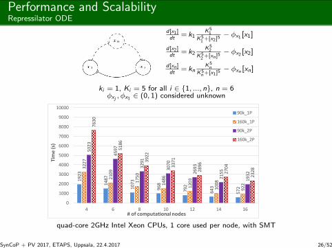
Performance and ScalabilityRepressilator ODE

d [x1]dt

= k1K5

1

K51 +[x2]5

− φx1 [x1]

d [x2]dt

= k2K5

2

K52 +[xn ]5

− φx2 [x2]

d [xn ]dt

= knK5n

K5n +[x1]5

− φxn [xn]

ki = 1, Ki = 5 for all i ∈ {1, ..., n}, n = 6φxj , φx1 ∈ (0, 1) considered unknown

1923

1487

1073

968

792

643

572

3227

2109

1750

1486

1203

1008

922

5023

4597

3291

3070

2693

2155

1932

7630

5186

3922

3371

2896

2704

2328

0

1000

2000

3000

4000

5000

6000

7000

8000

9000

10000

4 6 8 10 12 14 16

Tim

e (

s)

# of computational nodes

90k_1P

160k_1P

90k_2P

160k_2P

quad-core 2GHz Intel Xeon CPUs, 1 core used per node, with SMT


Outline

1 Motivation




5 Discussion


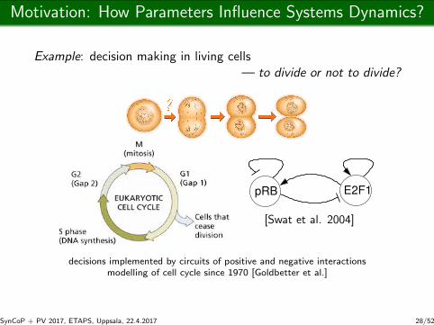
Motivation: How Parameters Influence Systems Dynamics?

Example: decision making in living cells— to divide or not to divide?

E2F1pRB

[Swat et al. 2004]

decisions implemented by circuits of positive and negative interactionsmodelling of cell cycle since 1970 [Goldbetter et al.]


Motivation: How Parameters Influence Systems Dynamics?Bifurcation Analysis of Dynamical Systems

typical phase portraits around equilibria:

bifurcation is defined as a topological change in phase space

small change in parameter =⇒ qualitative change in dynamicsthe goal of bifurcation analysis is to identify bifurcation points


Motivation: How Parameters Influence Systems Dynamics?Bifurcation Analysis in Systems Theory

cannot divide can decide for division must divide


Motivation: Models of Complex Dynamical SystemsUnderstanding Role of Parameters

in the vector field the equilbria have certain patterns

the patterns change with parameters (appear, disappear,change shape)

0 0,8 1,6 2,4 3,2 4 4,8 5,6 6,4 7,2 8 8,8 9,6 10,4 11,2 12 12,8 13,6 14,4 15,2 16 16,8 17,6 18,4 19,2

0,8

1,6

2,4

3,2

4

4,8

5,6

6,4

7,2

8

8,8

9,6

10,4

11,2

12

12,8

Insert text here

pRB

E2F1

0 0,8 1,6 2,4 3,2 4 4,8 5,6 6,4 7,2 8 8,8 9,6 10,4 11,2 12 12,8 13,6 14,4 15,2 16 16,8 17,6 18,4 19,2

0,8

1,6

2,4

3,2

4

4,8

5,6

6,4

7,2

8

8,8

9,6

10,4

11,2

12

12,8

Insert text here

pRB

E2F1

p = 0.006 p = 0.012


Phase Portrait SpecificationElementary Patterns

Single-state patterns

*

saddle

*

sink source flow

Multi-state patterns


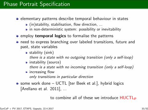
Phase Portrait Specification

elementary patterns describe temporal behaviour in states

(in)stability, stabilisation, flow direction, ...in non-deterministic system: possibility or inevitability

employ temporal logics to formalise the patterns

need to express branching over labeled transitions, future andpast, state variables

stability (sink)there is a state with no outgoing transition (only a self-loop)instability (source)there is a state with no incoming transition (only a self-loop)increasing flowonly transitions in particular direction

some work done – UCTL [ter Beek et al.], hybrid logics[Arellano et al. 2011], ...

to combine all of these we introduce HUCTLP


Phase Portrait Specification: HUCTLP

HUCTLP — hybrid UCTL with past

in addition to AP there are direction formulae:

χ ::= true | d | ¬χ | χ ∧ χ where d ∈ Dir

state formulae

ϕ ::= true | p | ¬ϕ | ϕ ∧ ϕ | Eψ | Aψ |Eψ | Aψ | x | ↓ x .ϕ | @x .ϕ | ∃x .ϕ

path formulae

ψ ::= Xχ ϕ | ϕ χUϕ | ϕ χUχ ϕ | ϕ χWϕ | ϕ χWχ ϕ


Phase Portrait Specification: HUCTLP

Single-state patterns

sink (stable steady state): ↓ s.AX s

source (only self-loops, no other incoming): ↓ s. AX s

2d-saddle (nort-south outgoing, west-east incoming):AXN∨S true ∧ EXN true ∧ EXS true∧AXE∨W true ∧ EXE true ∧ EXW true

Multi-state patterns

state in a nontrivial SCC: ↓ s.EX EF s

state in a final SCC (generalised sink): ↓ s.AG EF s

Relations among patterns

at least two sinks in the whole system:∃s.∃t.(@s.¬t ∧ AX s) ∧ (@t.AX t)


Phase Portrait SpecificationFrom Phase Portrait Specification to Parametric Phase Portrait

phase portrait specification φ = {ϕ1, ϕ2}phase portrait pattern Xφ = {ϕ1 ∧ ϕ2, ϕ1 ∧ ¬ϕ2,¬ϕ1 ∧ ϕ2,¬ϕ1 ∧ ¬ϕ2}

subpatterns, e.g., X ′ = {¬ϕ1 ∧ ϕ2,¬ϕ1 ∧ ¬ϕ2} ⊂ Xφ

ϕ1 ∧ ¬ϕ2

ϕ1 ∧ ϕ2

¬ϕ1 ∧ ϕ2

¬ϕ1 ∧ ¬ϕ2

ϕ2

¬ϕ2

Parametric Phase Portrait

parameter space PP(ϕ) ⊆ P all parameters for which there is a state satisfying ϕ

stratum: ΓXφ =⋂ϕ∈Xφ P(ϕ), ΓX ′ =

⋂ϕ∈X ′ P(ϕ), . . .

p ∈ P is a bifurcation point if it is a boundary point of some stratum


Discrete Bifurcation Analysis Problem

Problem Definition

Assume P is a finite partially ordered domain representing them-dimensional parameter space. Given a parameterised modelM and a phase portrait specification φ, compute the parametricportrait of M wrt φ and identify all bifurcation points in P wrtM and φ.

Parametrised Model M

Phase Portrait Specification φ

ColouredModel

Checking

Parametric Portrait Bifurcation Points


Outline

1 Motivation




5 Discussion


Case study: Biodegradation of Trichloropropane in E. coli

TCP DCP ECH CPD GDL GLYDhaA HheC EchA HheC EchA

d [TCP]dt

=− k1·DhaA·[TCP]Km,1+[TCP]

d [DCP]dt

= k1·DhaA··[TCP]Km,1+[TCP]

− k2·HheC ·[DCP]Km,2+[DCP]

d [ECH]dt

= k2·HheC ·[DCP]Km,2+[DCP]

− k3·EchA·[ECH]Km,3+[ECH]

d [CPD]dt

= k3·EchA·[ECH]Km,3+[ECH]

− k4·HheC ·[CPD]Km,4+[CPD]

d [GDL]dt

= k4·HheC ·[CPD]Km,4+[CPD]

− k5·HheC ·[GDL]Km,5+[GDL]

d [GLY ]dt

= k5·HheC ·[GDL]Km,5+[GDL]

biodegradation of toxic substrate and intermediates

synthetic pathway utilising enzymes from two other bacteriaRhodococcus rhodochrous NCIMB 13064; Agrobacterium radiobacter AD1

find optimal enzymes concentration balancing metabolicburden and toxicity



Desired behaviour:

“TCP is finally completely degraded and the concentration of intermediates does notexceed given bounds”

Formally:

ϕ1 = (A([TCP] > x)U(AF(AG [TCP] < y))),

ϕ2 = (A([GLY ] < y)U(AF(AG [GLY ] > x))),

ϕ3 = (AG [DCP] < v) ∧ (AG [GDL] < w),

ϕ = (ϕ1 ∧ ϕ2 ∧ ϕ3),

where x , y , v and w are estimated values making an instance of this property:

x = 1.9 (according to authors1 using the value 2 mM),

y = 0.01 (obviously, cannot be zero),

v ∈ {0.5, 0.3, 0.1} (variations based on experimental data observation)

w ∈ {0.5, 0.25, 0.1} (variations based on experimental data observation)

1Kurumbang et al., ACS Synthetic Biology, 2013SynCoP + PV 2017, ETAPS, Uppsala, 22.4.2017 41/52


DhaA

HheC

EchA

DhaA

Hh

eC

DhaA

Ech

A

HheC

Ech

A

A sample of the resulting parameter space for a particular initial state:TCP ∈ [1.9, 1.9586], DCP ∈ [0.448898, 0.5], GDL ∈ [0.0, 0.0669138], GLY ∈ [0.0, 0.01]

Dotted area corresponds to ϕ (v = 0.5, w = 0.25).SynCoP + PV 2017, ETAPS, Uppsala, 22.4.2017 42/52

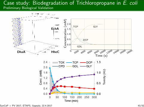
Case study: Biodegradation of Trichloropropane in E. coliPreliminary Biological Validation

DhaA HheC

EchA

Time (s)

Co

nce

ntr

ati

on

(mM

)

2.0

1.5

1.0

0.5

0.0

02000

40006000

800010000

1200014000

1600018000

TCP GLY

DCP

GDL


Outline

1 Motivation




5 Discussion


Case Study: Regulation of G1/S Cell Cycle Transition

E2F1pRB

[Swat et al. 2004]

d [pRB]dt

= k1[E2F1]

Km1+[E2F1]J11

J11+[pRB]− φpRB [pRB]

d [E2F1]dt

= kp + k2a2+[E2F1]2

K2m2+[E2F1]2

J12J12+[pRB]

− φE2F1[E2F1]

bifurcation analysis wrt φpRB

Analysed phase portrait pattern:

• ϕ1 := ∃s.∃t.(@s.AG EF s)∧ (@t.¬EF s ∧AG EF t)∧E¬NF s ∧E¬SF t

• ϕ2 := ¬ϕ1 ∧ ↓ s.AG EF s ∧ E2F1 < 4

• ϕ3 := ¬ϕ1 ∧ ↓ s.AG EF s ∧ E2F1 > 4SynCoP + PV 2017, ETAPS, Uppsala, 22.4.2017 45/52

Case Study: ResultsE

2F

1

pRB

ϕ2 ϕ1 ϕ3

φpRB = 0.0075 φpRB = 0.0115 φpRB = 0.014[0.002, 0.011] [0.011, 0.0136] [0.0136, 0.5]

bifurcation points: {0.011, 0.0136}

results agree with numerical methods up-to precision ofapproximation/discretisation


Outline

1 Motivation




5 Discussion


Summary and Conclusions

exploiting dynamical systems under parameter uncertainty byenumerative model checking with symbolic representation ofparameters

good scalability achieved for interval-based representation ofparameters

scalability of SMT-based version depends on model structure

remaining challenges:

approximation: explore errors, what can be guaranteed?abstraction: narrow the extent of overapproximation – canDarboux polynomials or barrier certificates help?improve scalabilityis it possible to combine model checking with simulation?[TCSB XIV, 2012]


Discussion

relations to parametric model checking

action synthesis [Knapik et al. 2014]entirely symbolic approachesin our case action parameters depend on states

bifurcation of programs/protocols

a form of robustness analysis

abstract interpretation wrt parameters

parameter space compaction


Check Out Pithya

https://github.com/sybila/pithya-gui


https://github.com/sybila/pithya-gui

Digital Systems Biology Laboratory

http://sybila.fi.muni.cz

since 2009

originated in model checking communityinvolved in systems biology since 2007 (EC-MOAN FP6)

parallel model checking algorithms development

adapting formal methods to applications in systems biologyformal specification and modelling of biological systemsparameter synthesis and bifurcation analysis

contributions to systems biology and bioinformaticsintegration of formal methods with bionformatics andexperimental biologycase studies with biological groups


http://sybila.fi.muni.cz

Credits

Computer Science

Lubos Brim, Marta Kwiatkowska, Thomas Henzinger,Loıc Pauleve, Ezio Bartocci, Luca Bortolussi, Jerome Feret,Andrzej Mizera, Alessandro Abate, Jan Van Schuppen, MilanCeska, Nikola Benes, Stefan Haar, Heike Siebert, Hidde de Jong

Biology

Ralf Steuer, Louis Mahadevan, Jan Cerveny, Dusan Lazar, PavelKrejcı, Stefanie Hertel, Christoff Flamm

Funding

Grant Agency of Czech Republic

C4SYS – National Infrastructure for Systems Biology


parameter synthesis in dynamical systems by model checking

Documents