the role of the confidence intervals in parameter ... · the role of the confidence intervals in...

1

The Role of the Confidence Intervals in Parameter Estimation and Model Refinement for Dynamical Systems

Mordechai Shacham, Chem. Eng. Dept., Ben-Gurion University, Beer-Sheva, Israel

Neima Brauner, School of Engineering, Tel-Aviv University, Tel-Aviv, Israel

Introduction Reliable mechanistic kinetic models of chemical/biological processes are essential for the understanding, design, optimization and control of such processes. Such models are often described by systems of ordinary differential equations (ODE's). The models usually contain unknown parameters that need to be determined using a set of measurements (experimental data). Typically, the estimation of the parameter values is performed using a maximum likelihood approach where the objective is to minimize the weighted squared error between the set of the measured data and the corresponding model prediction. The various stages of the mechanistic model development and the estimation of the model parameters in dynamic systems were described in detail by Maria (2004). Many methods have been developed in an attempt to find the global optimum of the parameter estimation problem for dynamic problems (for description of some recently developed methods and reviews of earlier methods see for example Dua, 2011, Michalic et al., 2009, and Esposito and Floudas, 2000). Test problems for evaluation of the methods for their global convergence ability and for computational efficiency were proposed for example by Biegler et al., 1986, Floudas et al., 1999 and Moles et al. 2013. Many of these test problems, however, disregard some of the major difficulties involved in the tasks of the mechanistic model development and parameter identification. Consider for example the test problem presented by Moles et al. 2013. This test problem consists of the estimation of 36 kinetic parameters of a nonlinear biochemical model formed by 8 ODE's (ordinary differential equations) that describe the variation of the metabolite concentration with time. "Pseudo" experimental data for this test problem was generated by introducing a "nominal" set of parameter values into the model, integrating the model equations and recording the "experimental" values at 20 equally spaced time intervals. No measurement noise was added to the simulated experimental data. This test problem has proven to be quite challenging because of the high dimensionality and the large number of local solutions, however it represents oversimplification in many aspects related to practical problems. In this test problem there is no uncertainty regarding the adequacy of the mathematical model to the process, as the "process" data is actually generated by the model, large amount and high precision "experimental" data, as well as a good set of references for initial guesses for the parameters (i.e., the parameter values that were used to generate the data) are available. Test problems which are more realistic in terms of the postulated mathematical model of the process and the available data are presented, for example, by Biegler et al. (1986), Maria (1989) and Zamostny and Belohlav (1999). These problems are characterized by uncertainty regarding the suitability of the mathematical model to represent the data, availability of insufficient amount and/or low precision noisy experimental data and lack of sensible initial estimates for some (or all) of the parameter values. The uncertainty of the adequacy of the model may require modification of the model in a "trial and error" fashion. The combination of non-linear models and insufficient and/or low precision experimental data may reduce the

2

reliability of statistical measures. Inappropriate initial estimates for the parameter values may cause failure of the ODE integration algorithms (because of extreme stiffness of the ODE's), or no convergence to a global minimum. Usually, the parameters that need to be identified have clear physical significance. For example the parameters of the test problem presented by Biegler et al. (1986) include activation energies, preexponential factors in rate constants, equilibrium constants and heteroscedasticity parameters. It is important to find reliable estimates for as many of the parameters as possible, as the mathematical model and the estimated parameter values will eventually be used for various purposes, such as process scale-up, design etc. In realistic problems, finding reliable estimates for as many parameters as possible may involve the use of different solution approaches (simultaneous and/or sequential), different minimization techniques (gradient based or direct search) and the use of non-scaled or normalized variables in the objective function. The analysis of the results must be based on statistical metrics (such as the confidence interval) and visual comparison of the calculated curves with the experimental data (in addition to ensuring the achievement of the global minimum of the objective function). Our proposed approach for reliable estimation of as many parameters as possible given a particular model and a set of experimental data will be demonstrated using the example presented by Maria (1989). The various solution and analysis techniques that are used to achieve the above stated goal are described in the following section. Basic Concepts Adopting the terminology used by Floudas et al., 1999, the parameter estimation problem involving an ODE model can be formulated as follows:

( ) ( )i

n m

i

c

iiWxx *

2

1 1

,,min ∑∑Φ= =

−=µ

µµ

θ

θ (1)

s.t.

( )

0)0(

,,

zz

zFz

=

= tdt

dθ

(2)

where F is a system of m ordinary differential equations, z is a vector of m dynamic variables, θ

is a vector of p parameters, xµ is a vector of m observed values (of z ) at the µth data point, c

µx

is a vector of m calculated variable values at the µth data point and W is a vector of m weighting factors. An alternative formulation which enables converting the differential parameter estimation problem into an algebraic parameter estimation problem is the following.

( ) ( )i

n m

i

c

iiWxx '*''

2

1 1

,,'min ∑∑Φ= =

−=µ

µµ

θ

θ (3)

s.t.

( ), , tµ µ θ′ =x F x nK,2,1=µ (4)

3

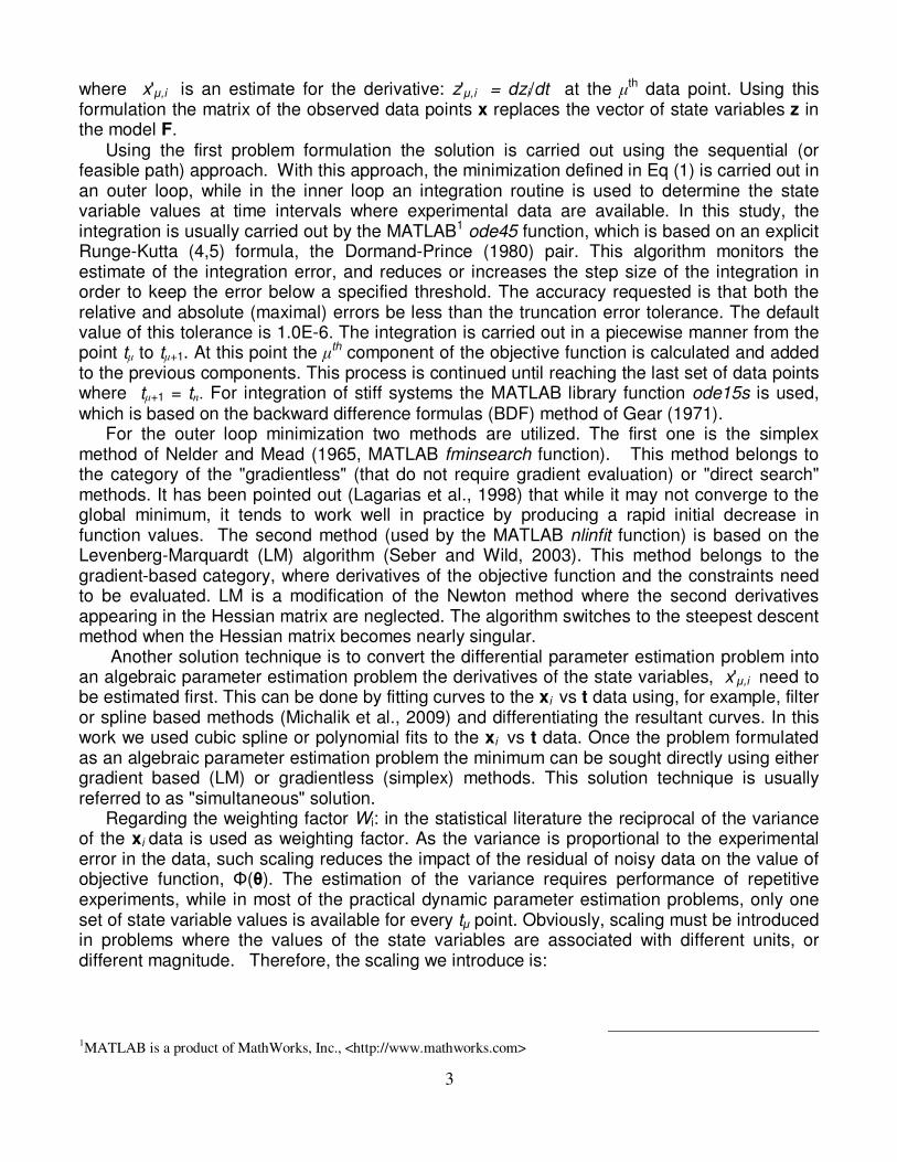
where x'µ,i is an estimate for the derivative: z'µ,i = dzi/dt at the µth data point. Using this formulation the matrix of the observed data points x replaces the vector of state variables z in the model F. Using the first problem formulation the solution is carried out using the sequential (or feasible path) approach. With this approach, the minimization defined in Eq (1) is carried out in an outer loop, while in the inner loop an integration routine is used to determine the state variable values at time intervals where experimental data are available. In this study, the integration is usually carried out by the MATLAB1 ode45 function, which is based on an explicit Runge-Kutta (4,5) formula, the Dormand-Prince (1980) pair. This algorithm monitors the estimate of the integration error, and reduces or increases the step size of the integration in order to keep the error below a specified threshold. The accuracy requested is that both the relative and absolute (maximal) errors be less than the truncation error tolerance. The default value of this tolerance is 1.0E-6. The integration is carried out in a piecewise manner from the point tµ to tµ+1. At this point the µth component of the objective function is calculated and added to the previous components. This process is continued until reaching the last set of data points where tµ+1 = tn. For integration of stiff systems the MATLAB library function ode15s is used, which is based on the backward difference formulas (BDF) method of Gear (1971). For the outer loop minimization two methods are utilized. The first one is the simplex method of Nelder and Mead (1965, MATLAB fminsearch function). This method belongs to the category of the "gradientless" (that do not require gradient evaluation) or "direct search" methods. It has been pointed out (Lagarias et al., 1998) that while it may not converge to the global minimum, it tends to work well in practice by producing a rapid initial decrease in function values. The second method (used by the MATLAB nlinfit function) is based on the Levenberg-Marquardt (LM) algorithm (Seber and Wild, 2003). This method belongs to the gradient-based category, where derivatives of the objective function and the constraints need to be evaluated. LM is a modification of the Newton method where the second derivatives appearing in the Hessian matrix are neglected. The algorithm switches to the steepest descent method when the Hessian matrix becomes nearly singular. Another solution technique is to convert the differential parameter estimation problem into an algebraic parameter estimation problem the derivatives of the state variables, x'µ,i need to be estimated first. This can be done by fitting curves to the xi vs t data using, for example, filter or spline based methods (Michalik et al., 2009) and differentiating the resultant curves. In this work we used cubic spline or polynomial fits to the xi vs t data. Once the problem formulated as an algebraic parameter estimation problem the minimum can be sought directly using either gradient based (LM) or gradientless (simplex) methods. This solution technique is usually referred to as "simultaneous" solution. Regarding the weighting factor Wi: in the statistical literature the reciprocal of the variance of the xi data is used as weighting factor. As the variance is proportional to the experimental error in the data, such scaling reduces the impact of the residual of noisy data on the value of objective function, Φ(θ). The estimation of the variance requires performance of repetitive experiments, while in most of the practical dynamic parameter estimation problems, only one set of state variable values is available for every tµ point. Obviously, scaling must be introduced in problems where the values of the state variables are associated with different units, or different magnitude. Therefore, the scaling we introduce is:

1MATLAB is a product of MathWorks, Inc., <http://www.mathworks.com>

4

iixW ,max/1 µ

µ

= (5)

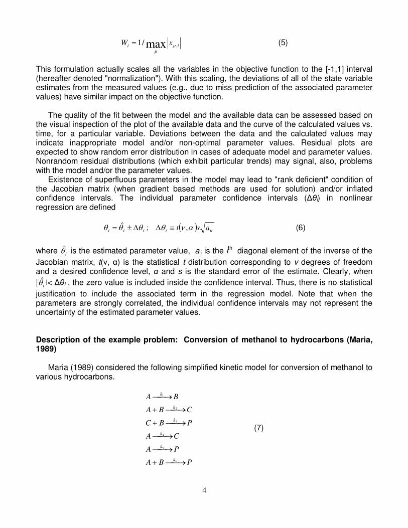
This formulation actually scales all the variables in the objective function to the [-1,1] interval (hereafter denoted "normalization"). With this scaling, the deviations of all of the state variable estimates from the measured values (e.g., due to miss prediction of the associated parameter values) have similar impact on the objective function. The quality of the fit between the model and the available data can be assessed based on the visual inspection of the plot of the available data and the curve of the calculated values vs. time, for a particular variable. Deviations between the data and the calculated values may indicate inappropriate model and/or non-optimal parameter values. Residual plots are expected to show random error distribution in cases of adequate model and parameter values. Nonrandom residual distributions (which exhibit particular trends) may signal, also, problems with the model and/or the parameter values. Existence of superfluous parameters in the model may lead to "rank deficient" condition of the Jacobian matrix (when gradient based methods are used for solution) and/or inflated confidence intervals. The individual parameter confidence intervals (∆θi) in nonlinear regression are defined

( )iiiiii

ast ανθθθθ ,;ˆ ≡∆∆±= (6)

where iθ̂ is the estimated parameter value, aii is the ith diagonal element of the inverse of the

Jacobian matrix, t(ν, α) is the statistical t distribution corresponding to v degrees of freedom and a desired confidence level, α and s is the standard error of the estimate. Clearly, when

|iθ̂ |< ∆θi , the zero value is included inside the confidence interval. Thus, there is no statistical

justification to include the associated term in the regression model. Note that when the parameters are strongly correlated, the individual confidence intervals may not represent the uncertainty of the estimated parameter values.

Description of the example problem: Conversion of methanol to hydrocarbons (Maria, 1989) Maria (1989) considered the following simplified kinetic model for conversion of methanol to various hydrocarbons.

PBA

PA

CA

PBC

CBA

BA

k

k

k

k

k

k

→+

→

→

→+

→+

→

6

5

4

3

2

1

(7)

5

where A represents the oxygenates, B is the intermediate 2HC&& , C represents the olefins, and

P represents the paraffins, aromatics and other products. The model of the reaction is formulated under the assumption of simple kinetics and quasi- steady state for B.

( )

14

2152

152113

13

2152

212112

143

2152

211

1

)(

)(

)(

)(

)2(

xxx

xxx

dt

dx

xxx

xxx

dt

dx

xxx

x

dt

dx

θθθ

θθ

θθθ

θθ

θθθθ

θθ

+++

−=

+++

−=

++++

−−=

(8)

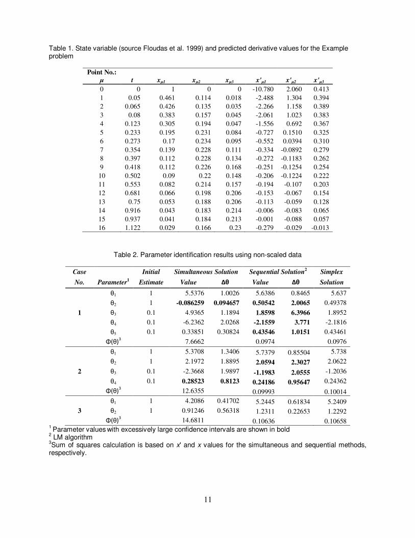
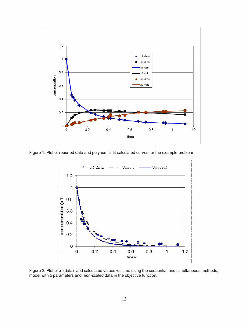
where x1, x2 and x3 are the mole fractions of A, B and C respectively. The parameter vector θ is defined as: θ = [k1, k2/k3 k4, k5, k6/k3]. The available state variable data vs. time (as reported by Floudas et al., 1999) are shown in Table 1. The data for this problem originated from Maria (1989) who points out that only four of the reported data points are experimental and the additional 12 points are approximated by splines. The first experimental point is point No. 9 at t = 0.418 s. In order to use the simultaneous solution method, estimates for the time derivatives of the state variables: x'1 ≡ dx1/dt; x'2 ≡ dx2/dt and x'3 ≡ dx3/dt are needed. To this aim, smooth curves need to be fitted to the data and subsequently differentiated. We tried to fit different type of curves (mainly cubic splines). The best results were obtained using smoothing polynomials, 5th degree polynomials for x1 and x2 and a 2nd degree polynomial (passing through the origin) for x3. The regression program of Polymath2 was used to fit the polynomials. The reported data and the calculated polynomial curves are shown in Figure 1. The fit between the polynomial curves and the data appears to be satisfactory. The derivatives values obtained by differentiating the polynomial curves are shown in Table 1. Identifying the optimal model and parameter values using non-scaled variable values In kinetic models where all the state variables are the mole fractions, apparently scaling of the variables is not necessary and was not introduced in previous studies that attempted to solve the above problem. Therefore, to enable comparison with the reported optimal solutions (Maria, 1989, Floudas et al., 1999, Eposito and Floudas, 2000) in the following analysis, first, no weights were assigned to the data and calculated values of the state variables included in the objective function. The problem was solved using the simultaneous (LM algorithm) and sequential (LM and Simplex algorithms) methods for various numbers of the parameters. The results of this study are summarized in Tables 2 and 3. In all the cases the initial estimates used for the parameter values were: θ1,0 = θ2,0 =1 and θ3,0 = θ4,0 = θ5,0 = 0.1. This set of initial estimates was selected arbitrarily. Case 1- Let us consider the results of Case 1 (where all 5 parameters are included in the model) and the LM sequential solution technique was used for solution. For this case it took 128 function evaluations (integration of the complete set of differential equations, Eq. 2) and

2 Polymath is a product of Polymath Software, <http://www.polymath-software.com>

6

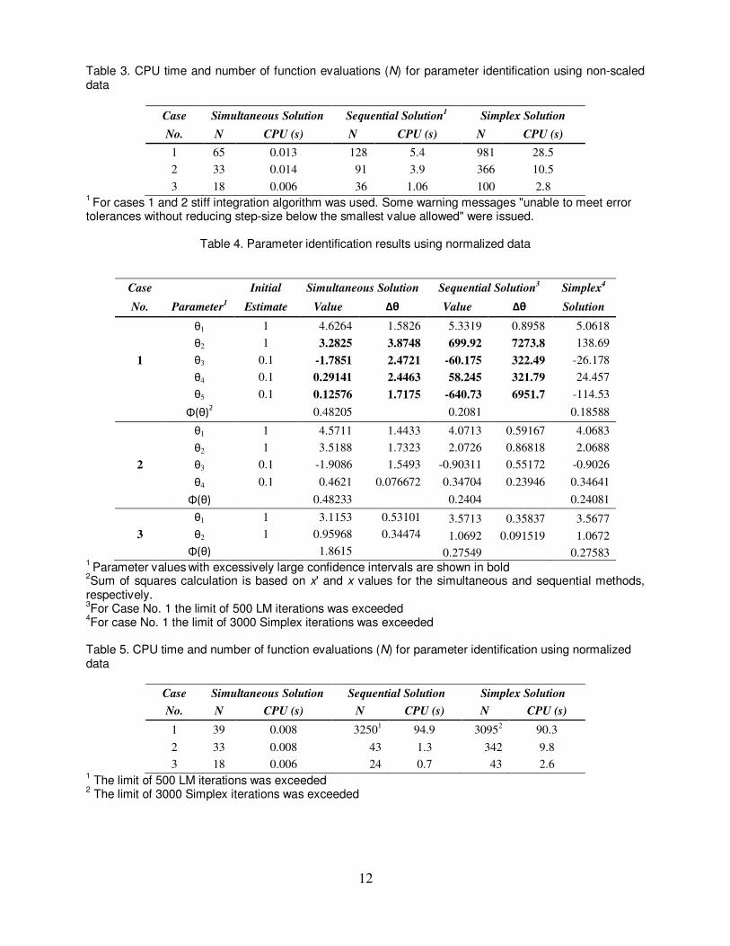
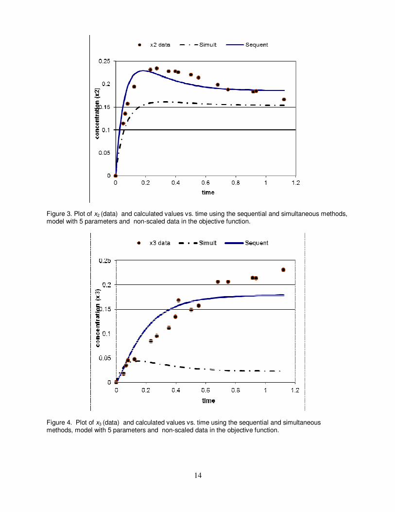
5.4 CPU seconds (Table 3) to reach the solution. Some of the θ values encountered in the path to the optimal solution rendered the ODE system stiff, requiring the use of a stiff solution technique and relaxation of the local truncation error tolerance. However near the optimal solution non-stiff integration algorithm could be used. The solution obtained is θ =(5.6386, 0.50542, 1.8598, -2.1559, 0.43546) with objective function value of Φ(θ) = 0.0974. Comparing the θi and the respective ∆θi values reveals that only θ1 is significantly different from zero. For the rest of the parameters the confidence interval (∆θi ) is greater in absolute value than the parameter (θi), indicating that the 5 parameters model is unstable and one or more of the parameter values can be set to zero. Using the Simplex sequential solution technique for Case 1 yields parameter values very similar to values obtained by the LM algorithm (Table 2) with a slightly higher objective function value (Φ(θ) = 0.0976). In terms of the computational effort required, the Simplex method is much less efficient compared to the LM algorithm, requiring 981 function evaluations and 28.5 CPU seconds to converge. The simultaneous solution technique is computationally much more efficient than the sequential techniques. The convergence for Case 1 required 65 function evaluations and 0.013 CPU seconds. Thus, for this problem, the function evaluation that numerical integration takes ~ 200 times longer than the evaluation of the derivatives that requires only substitution of the values into the model equations. As for the parameter values obtained by the simultaneous solution technique, the value of θ1 = 5.5376, is very close to the value obtained by the sequential methods. However, the rest of the parameter values are entirely different. Observe, for example, that the value for θ2 is negative (θ2 = -0.086259), while the sequential techniques yielded positive value for this parameter. Checking the confidence interval for this parameter shows, also, that θ2 is not significantly different from zero. The objective function value is Φ(θ) = 7.6662, but it cannot be compared with the values obtained for the sequential methods, as the objective function in this case involves derivative values that vary in a much wider range (-10.8 to 2.06) compared to the range of the state variable values (0 to 1). Figures 2, 3 and 4 show the mole fraction data and the calculated values vs. time for x1, x2 and x3, respectively. Included are the calculated values obtained using the parameter values shown as Case 1 in Table 2 for the simultaneous and the sequential methods (using the LM algorithm). The calculated values of the Simplex method cannot be distinguished from the LM method and can be practically considered the same as the latter. For x1 the range of the

available data is 0.029 ≤ x1 ≤ 1 and -10.78 ≤ 1x′ ≤ -0.279. For this variable both calculated

curves match satisfactorily the data (Fig 2). For x2 the range of the available data is 0.0 ≤ x2 ≤

0.234 and -0.1254 ≤ 2x′ ≤ -2.06. For this variable there are considerable deviations between

the data and the calculated curves (larger deviation for the curve calculated by the simultaneous method) starting at about t = 0.1. For x3 the range of the available data is 0.0 ≤ x3

≤ 0.214 and -0.013 ≤ 3x′ ≤ 0.413. In this case the representation of the data by the sequential

method curve is fair, while the representation by the simultaneous method curve is completely wrong starting at about t = 0.1. The poor performance of the simultaneous method for predicting x2 and x3 can be explained by the smaller absolute values of their derivatives, which may make the contribution of their residual to Φ(θ) insignificant. Case 2- Since the use of 5 parameters in the mathematical model leads to some parameter values which are not significantly different from zero the number of parameters needs to be reduced. First, let us try to remove the parameter θ5 from the model as in all (except one) cases it appears paired with θ2. The results obtained by setting θ5 = 0 appear as Case No. 2 in

7

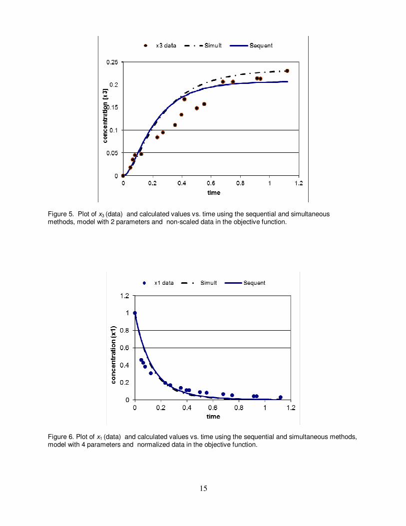
Tables 2 and 3. Observe that the reduction of the number of parameters reduces the number of function evaluations for reaching the solution. The largest savings is in the computational effort for the Simplex solution method, followed by the sequential LM solution method and finally the simultaneous LM solution method. Except for θ1 there are considerable changes in the parameter values in comparison to Case 1. The parameter values obtained using the Simplex and the sequential LM solution methods are very close and the ∆θ values for the parameters θ1, θ2 and θ3 are still larger in absolute value than the parameter values. The parameter values obtained by the simultaneous method are closer now to the values obtained by the other methods than in Case 1, yet the value of θ4 is not significantly different from zero. Observe that the objective function values are higher for the 4 parameter optimal solutions than for the 5 parameter optimal solution. Case 3- The parameter values obtained for the model containing two parameters ( θ1 and θ2 ) using non-weighted variables in the objective function, is considered the optimal one by, for example, Maria, 1989, Floudas et al., 1999 and Eposito and Floudas, 2000. This solution is presented as Case 3 in Table 2. The optimal parameter values obtained using the LM sequential solution method is θ1 = 5.2445 and θ2 = 1.2311 with Φ(θ) = 0.10636. The solution presented by Floudas et al., 1999 is: θ1 = 5.2407, θ2 = 1.2176 and Φ(θ) = 0.10693, thus the values are identical up to three decimal digits (except for θ2, where only two digits are identical). The parameter values obtained by the simultaneous method (θ1 = 4.2086 and θ2 = 0.91246) are much closer to the sequential solution values than in the 5 and 4 parameter cases. The two parameter solutions are stable and all the ∆θ values are smaller in absolute value than the corresponding parameter values. The objective function values are higher than for the four and five parameter cases. In spite of that, the two parameters model represents the data much better than, say, the five parameters model. This is demonstrated in Fig. 5 for the concentration, x3. Comparing this plot with the 5 parameters results of Fig. 4 shows that the calculated curves of the 2 parameters model obtained by both the sequential and the simultaneous techniques represent the x3 data much better than the 5 parameters model. Regarding the computational effort required, there is a reduction by factors of ~2 to ~4 in the number of function evaluations and CPU time, relatively to the 4 parameters model. There was no need to use the stiff integration algorithm with the LM based sequential solution technique as in the 4 and 5 parameters models. However, removal of 3 of the model parameters means in this case that no estimate can be obtained for the value some of the kinetic constants (k4, k5 and k6/k3). Identifying the optimal model and parameter values using normalized variable values Based on the absolute maximal data values, the following weight (normalization) factors were specified for the three variables: W1 = 1, W2 = 1/0.234 = 4.2735 and W3 = 1/0.214 = 4.6729. The weight factors obtained for the derivative values are: W '1 = 1/ 10.78 = 0.092764, W '2 = 1/2.06 = 0.48544 and W '3 = 1/0.413 = 2.4213. The complete study described in the previous section was repeated using normalized data and variables. The results of this study are summarized in Tables 4 and 5. Case 1- Let us consider first the LM sequential solution for the 5 parameter case. This method did not converge within 500 iterations (3250 function evaluation, see Table 5). The results presented in Table 4 show that the minimum in this case is unbounded. Only the value of θ1 is similar to the value obtained for the non-normalized case (θ1 = 5.3319 instead of 5.6386) but θ2

8

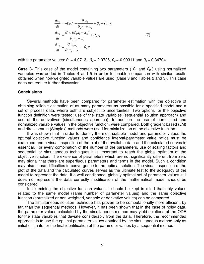
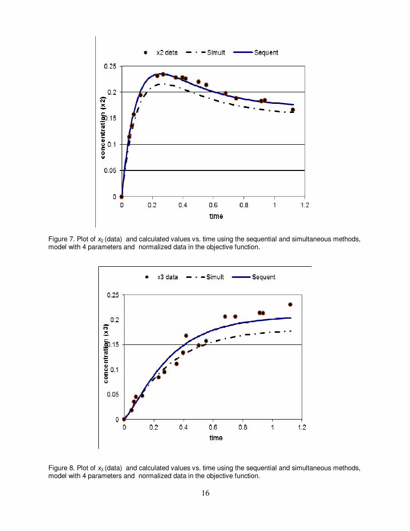
and θ4 obtain very large positive values (for example θ2 = 699.92), while at the same time θ3 and θ5 obtain increasing negative values. Still the objective function value is low: Φ(θ) = 0.2081. Comparing with the objective function value obtained when using non-scaled data, (Φ(θ) = 0.0974), while taking into account that weighting factors < 4 for the variables x2 and x3 are used in the present case, shows that the values are, at least, comparable. For the four parameters (except θ1) the confidence intervals are larger in absolute value than the corresponding parameters and obtain huge values. Thus, the 5 parameter model is highly ill- conditioned when normalized variables are used for parameter identification. The Simplex solution for this case did not converge either (after 3000 iterations, 3095 function evaluation). The trend in the parameter values is similar to the trend in the LM sequential solution, but the absolute values of the unbounded variables remain smaller and the objective function value is lower (Φ(θ) = 0.18588). The simultaneous solution technique did converge for this case after 39 function evaluations. However, for the last four parameters the confidence intervals are larger in absolute value than the corresponding parameters, implying again the existence of redundant parameters (and terms) in the kinetic model equations. Case 2- By setting θ5= 0, all the solution techniques converged to stable solutions within relatively small number of function evaluation. By the LM sequential method the following optimal parameter values are obtained: θ =(4.0713±0.59167, 2.0726±0.86818, -0.90311±0.55172, 0.34704±0.23946) with objective function value of Φ(θ) = 0.2404. Observe that although Φ(θ) is larger than for the 5 parameters solution, all the confidence intervals are now smaller than the corresponding parameter values. The Simplex solution for the parameter values matches the LM sequential solution up to two decimal digits. As for the simultaneous solution results, the parameter values obtained are different from the sequential solution values, by ~10% for θ1 and up to ~110% for θ3. In Figures 6, 7 and 8 the concentration data and calculated values vs. time are shown for x1, x2 and x3 respectively. The calculated values obtained using normalized variables and the four parameters models are displayed. For x1 (Fig. 6), the calculated curves of the sequential and simultaneous solutions match perfectly while the deviation from the data is somewhat smaller than for the results shown in Figure 2. For x2 (Fig. 7), there is a perfect match between the data and the calculated curves obtained by the sequential methods. The calculated curve obtained using the simultaneous method deviates up to 7% from the data for higher t values. The plot of x3 (Fig. 8) reveals that the data spread for this variable is such that it cannot be matched exactly by one curve. However, it seems that the sequential solution curve provides the best fit to the data (at large t in particular), while the simultaneous solution fits better the data at intermediate t. . It can be concluded that based on the comparison between the available data and the calculated curves, the model with the four parameters θ1, θ2, θ3, θ4, whose values are determined using a sequential solution technique with normalized (scaled) values in the objective function, represent best the process data. Testing the confidence interval and parameter value ratios for this solution shows that in this case all the parameter values are significantly different from zero. Thus, the most appropriate model identified based on the available data is:

9

14

212

2113

13

212

212112

143

212

211

1

)(

)2(

xxx

xx

dt

dx

xxx

xxx

dt

dx

xxx

x

dt

dx

θθ

θ

θθ

θθ

θθθ

θθ

++

=

++

−=

+++

−−=

(7)

with the parameter values: θ1 = 4.0713, θ2 = 2.0726, θ3 =-0.90311 and θ4 = 0.34704. Case 3- This case of the model containing two parameters ( θ1 and θ2 ) using normalized variables was added in Tables 4 and 5 in order to enable comparison with similar results obtained when non-weighted variable values are used (Case 3 and Tables 2 and 3). This case does not require further discussion. Conclusions Several methods have been compared for parameter estimation with the objective of obtaining reliable estimation of as many parameters as possible for a specified model and a set of process data, where both are subject to uncertainties. Two options for the objective function definition were tested: use of the state variables (sequential solution approach) and use of the derivatives (simultaneous approach). In addition the use of non-scaled and normalized variable values in the objective function, were compared. Both gradient based (LM) and direct search (Simplex) methods were used for minimization of the objective function. It was shown that in order to identify the most suitable model and parameter values the optimal objective function values and confidence interval-parameter value ratios must be examined and a visual inspection of the plot of the available data and the calculated curves is essential. For every combination of the number of the parameters, use of scaling factors and sequential or simultaneous techniques it is important to reach the global optimum of the objective function. The existence of parameters which are not significantly different from zero may signal that there are superfluous parameters and terms in the model. Such a condition may also cause difficulties in convergence to the optimal solution. The visual inspection of the plot of the data and the calculated curves serves as the ultimate test to the adequacy of the model to represent the data. If a well-conditioned, globally optimal set of parameter values still does not represent the data correctly modification of the mathematical model should be considered. In examining the objective function values it should be kept in mind that only values related to the same model (same number of parameter values) and the same objective function (normalized or non-weighted, variable or derivative values) can be compared. The simultaneous solution technique has proven to be computationally more efficient, by far, than the sequential methods. However, it has been shown that in the case of noisy data, the parameter values calculated by the simultaneous method may yield solutions of the ODE for the state variables that deviate considerably from the data. Therefore, the recommended approach is to use the optimal parameter values obtained by the simultaneous method only as initial estimate for the final identification of the parameter values by a sequential method.

10

References

1. Biegler, L. T., Damiano, J. J. and Blau, G. E. (1986) Nonlinear parameter estimation: a case study

comparison. AlChE Journal 32(1), 29-45. 2. Dormand, J. R. and P. J. Prince, "A family of embedded Runge-Kutta formulae," J. Comp. Appl.

Math., Vol. 6, 1980, pp 19-26. 3. Dua, V. (2011). An Artificial Neural Network approximation based decomposition approach for

parameter estimation of system of ordinary differential equations. Computers and Chemical Engineering 35, 545–553.

4. Esposito, W. R. and Floudas, C.A. (2000). Global optimization for the parameter estimation of differential-algebraic systems. Ind. Eng. Chem. Res. 39, 1291-1310.

5. Floudas, C. A., Pardalos, P. M., Adjiman, C. S., Esposito, W. R., Gümüs, Z. H., Harding, S.T., Klepeis, J. L., Clifford A. Meyer, C. A. and Schweiger, C. A. (1999). Handbook of Test Problems in Local and Global Optimization, Kluwer, Dordrecht, The Netherlands

6. Gear, C. W., Numerical Initial Value Problems in Ordinary Differential Equations, Prentice Hall, Englewood Cliffs, 1971

7. Lagarias, J. C., Reeds, J. A., Wright, M. H.and Wright, P. E. (1998). Convergence properties of the Nelder-Mead simplex method in low dimensions. Siam J. Optim. 9, (1), 112-147.

8. Leppävuori, J. T.; Domach, M.M.; Biegler, L.T., Parameter Estimation in Batch Bioreactor Simulation Using Metabolic Models: Sequential Solution with Direct Sensitivities, Ind. Eng. Chem. Res. 2011, 50, 12080-12091

9. Maria, G., An adaptive strategy for solving kinetic model coccomitant estimation-reduction problems., Can. J. Chem. Eng. 67, 825(1989)

10. Maria G. (2004). A Review of Algorithms and Trends in Kinetic Model Identification for Chemical and Biochemical Systems. Chem. Biochem. Eng. Q. 18 (3) 195–222.

11. Michalik, C.; Chachuat, B.; Marquardt, W., Incremental Global Parameter Estimation in Dynamical Systems, Ind. Eng. Chem. Res. 2009, 48, 5489–5497.

12. Moles, C. G., Mendes, P. and Banga, J. R. (2003). Parameter estimation in biochemical pathways: A comparison of global optimization methods. Genome Res. 13, 2467-2474.

13. Nelder, J.A. and Mead, R. “A Simplex Method for Function Minimization”, The Computer Journal, 7:308 (1965).

14. Seber, G. A. F., and C. J. Wild. Nonlinear Regression. Hoboken, NJ: Wiley-Interscience, 2003. 15. Tjoa, I.B. and Biegler, L. T. (1991). Simultaneous solution and optimization strategies for parameter

estimation of differential algebraic equation systems. Ind. Eng. Chem. Res. 30, 376-385. 16. Tjoa, I.B. and Biegler, L. T. (1992). Reduced successive quadratic programming strategy for errors-in-

variables estimation. Compurers chem. Engng, 16(6), 523-533.

11

Table 1. State variable (source Floudas et al. 1999) and predicted derivative values for the Example problem

Point No.:

µ t xµ1 xµ2 xµ3 x'µ1 x'µ2 x'µ3

0 0 1 0 0 -10.780 2.060 0.413

1 0.05 0.461 0.114 0.018 -2.488 1.304 0.394

2 0.065 0.426 0.135 0.035 -2.266 1.158 0.389

3 0.08 0.383 0.157 0.045 -2.061 1.023 0.383

4 0.123 0.305 0.194 0.047 -1.556 0.692 0.367

5 0.233 0.195 0.231 0.084 -0.727 0.1510 0.325

6 0.273 0.17 0.234 0.095 -0.552 0.0394 0.310

7 0.354 0.139 0.228 0.111 -0.334 -0.0892 0.279

8 0.397 0.112 0.228 0.134 -0.272 -0.1183 0.262

9 0.418 0.112 0.226 0.168 -0.251 -0.1254 0.254

10 0.502 0.09 0.22 0.148 -0.206 -0.1224 0.222

11 0.553 0.082 0.214 0.157 -0.194 -0.107 0.203

12 0.681 0.066 0.198 0.206 -0.153 -0.067 0.154

13 0.75 0.053 0.188 0.206 -0.113 -0.059 0.128

14 0.916 0.043 0.183 0.214 -0.006 -0.083 0.065

15 0.937 0.041 0.184 0.213 -0.001 -0.088 0.057

16 1.122 0.029 0.166 0.23 -0.279 -0.029 -0.013

Table 2. Parameter identification results using non-scaled data

Case Initial Simultaneous Solution Sequential Solution2

Simplex

No. Parameter1 Estimate Value Δθ Value Δθ Solution

θ1 1 5.5376 1.0026 5.6386 0.8465 5.637

θ2 1 -0.086259 0.094657 0.50542 2.0065 0.49378

1 θ3 0.1 4.9365 1.1894 1.8598 6.3966 1.8952

θ4 0.1 -6.2362 2.0268 -2.1559 3.771 -2.1816

θ5 0.1 0.33851 0.30824 0.43546 1.0151 0.43461

Φ(θ)3 7.6662 0.0974 0.0976

θ1 1 5.3708 1.3406 5.7379 0.85504 5.738

θ2 1 2.1972 1.8895 2.0594 2.3027 2.0622

2 θ3 0.1 -2.3668 1.9897 -1.1983 2.0555 -1.2036

θ4 0.1 0.28523 0.8123 0.24186 0.95647 0.24362

Φ(θ)3 12.6355 0.09993 0.10014

θ1 1 4.2086 0.41702 5.2445 0.61834 5.2409

3 θ2 1 0.91246 0.56318 1.2311 0.22653 1.2292

Φ(θ)3 14.6811 0.10636 0.10658

1 Parameter values

with excessively large confidence intervals are shown in bold

2 LM algorithm

3Sum of squares calculation is based on x' and x values for the simultaneous and sequential methods,

respectively.

12

Table 3. CPU time and number of function evaluations (N) for parameter identification using non-scaled data

Case Simultaneous Solution Sequential Solution1 Simplex Solution

No. N CPU (s) N CPU (s) N CPU (s)

1 65 0.013 128 5.4 981 28.5

2 33 0.014 91 3.9 366 10.5

3 18 0.006 36 1.06 100 2.8 1 For cases 1 and 2 stiff integration algorithm was used. Some warning messages "unable to meet error

tolerances without reducing step-size below the smallest value allowed" were issued.

Table 4. Parameter identification results using normalized data

Case Initial Simultaneous Solution Sequential Solution3 Simplex

4

No. Parameter1 Estimate Value Δθ Value Δθ Solution

θ1 1 4.6264 1.5826 5.3319 0.8958 5.0618

θ2 1 3.2825 3.8748 699.92 7273.8 138.69

1 θ3 0.1 -1.7851 2.4721 -60.175 322.49 -26.178

θ4 0.1 0.29141 2.4463 58.245 321.79 24.457

θ5 0.1 0.12576 1.7175 -640.73 6951.7 -114.53

Φ(θ)2 0.48205 0.2081 0.18588

θ1 1 4.5711 1.4433 4.0713 0.59167 4.0683

θ2 1 3.5188 1.7323 2.0726 0.86818 2.0688

2 θ3 0.1 -1.9086 1.5493 -0.90311 0.55172 -0.9026

θ4 0.1 0.4621 0.076672 0.34704 0.23946 0.34641

Φ(θ) 0.48233 0.2404 0.24081

θ1 1 3.1153 0.53101 3.5713 0.35837 3.5677

3 θ2 1 0.95968 0.34474 1.0692 0.091519 1.0672

Φ(θ) 1.8615 0.27549 0.27583 1 Parameter values

with excessively large confidence intervals are shown in bold

2Sum of squares calculation is based on x' and x values for the simultaneous and sequential methods,

respectively. 3For Case No. 1 the limit of 500 LM iterations was exceeded

4For case No. 1 the limit of 3000 Simplex iterations was exceeded

Table 5. CPU time and number of function evaluations (N) for parameter identification using normalized data

Case Simultaneous Solution Sequential Solution Simplex Solution

No. N CPU (s) N CPU (s) N CPU (s)

1 39 0.008 32501 94.9 30952 90.3

2 33 0.008 43 1.3 342 9.8

3 18 0.006 24 0.7 43 2.6 1 The limit of 500 LM iterations was exceeded

2 The limit of 3000 Simplex iterations was exceeded

13

Figure 1. Plot of reported data and polynomial fit calculated curves for the example problem

Figure 2. Plot of x1 (data) and calculated values vs. time using the sequential and simultaneous methods, model with 5 parameters and non-scaled data in the objective function.

14



15


Figure 6. Plot of x1 (data) and calculated values vs. time using the sequential and simultaneous methods, model with 4 parameters and normalized data in the objective function.

16



the role of the confidence intervals in parameter ... · the role of the confidence intervals in...

Documents