JOURNAL OF MATHEMATICAL ANALYSIS AND APPLICATIONS 84, 614-630 (198 I)

On the Existence of Global Smooth Solutions for a Model Equation for Fluid Flow in a Pipe

MITCHELL LUSKIN*

Department of Mathematics. The University of Michigan. Ann Arbor. Michigan 48109

Submitted bJ C. S. Morawetz

We model the flow of a fluid in a pipe by a first-order nonlinear hyperbolic system with zero-order nonlinear dissipation. We prove that a unique. global smooth solution exists if the initial data are in an appropriate invariant region and if the first derivatives of the initial data are suffkiently small.

1. INTRODUCTION

We consider here the existence of a global smooth (continuous) solution to the initial value problem for the quasilinear hyperbolic system modeling fluid flow in a pipe

pt + G, = 0, (x, t) E R x [O, 00).

.f-lGlG (l-1)

P(& 0) = P&h G(x, 0) = G,(x). x E P,

where p is mass density, G is momentum density, L’ = G/p is velocity, p = p@) is pressure, D is pipe diameter, and f is the “Moody” friction factor [ 10, pp. 288-2891. The friction factor is a function of the Reynolds number, Re E 1GI D/p, where ,U is the viscosity. Since D and ,u are to be treated as constants, we will consider f to be a function of 1Gj. We shall show that under realistic hypotheses on the equation of state, p =p@), and the friction factor,f-f(lGI), the system (1.1) has global smooth solutions if the initial data lie in appropriate invariant regions and if the first derivatives of the initial data are sufficiently small. This result is in contrast to the situation when there is no friction term present in (1.1). In that case, it is now well-

* Supported by AFOSR under Contract F49620-79-C-0149 and by a visiting professorship at the &ole Polytechnique Fed&ale, Lausanne. Switzerland.

614 0022~247><~81,!120614-17$02.00/O Copyright c, 1981 by Academic Press. Inc. All rights of reproduction in any form reserved.

GLOBALSMOOTH SOLUTIONS 615

known that discontinuities inevitably occur unless the initial data satisfy very restrictive conditions [6].

There is considerable practical interest in obtaining numerical approx- imations to the solution of (1.1). Knowing that the solution is smooth allows one to take advantage of efficient, high-order schemes which may be inap- propriate for solutions with discontinuities. Previous analyses of numerical methods for (1.1) have assumed the existence of smooth solutions [3, 71. In fact, the global existence of the approximate finite element solutions proposed in [3, 71 has been obtained by showing that the approximate solution is always in a neighborhood of a smooth solution to the differential problem.

Earlier work on the existence of global smooth solutions for quasilinear hyperbolic equations with lower-order dissipation has been done by Nishida [8]. Our work generalizes the form of the dissipation considered by Nishida. Nishida’s theory allowed only linear dissipation, i.e., -fl G 1 G/2Dp in (1.1) is replaced by -fG wherepis a positive constant. Since the “Moody” friction factor is discontinuous (multiple valued) when the flow changes from laminar to turbulent, we treat the case of discontinuous (multiple valued)

Also. we are able to replace Nishida’s requirement that the initial data lie in appropriate “sufficiently small” neighborhoods by the requirement that the initial data need only lie in an appropriate invariant region. This improvement in the analysis allows the application of our results to problems where the initial data can vary over ranges which are realistic for fluid flow problems of practical interest in engineering, such as the modeling of gas and oil pipelines.

2. DEFINITIONS AND STATEMENT OF THEOREM

The definitions and hypotheses for our theorem given in this section are illustrated by the example in Section 5. We assume that p(p) E C’(IF’ +). Furthermore, we guarantee the hyperbolicity of (1.1) by assuming that p’@)>OforpERfandwesety@)=@@

We turn to the friction factor and set F(G) =fl G / G/ZD. For fixed G, > 0 (the critical flow rate at which the transition from laminar to turbulent takes place), we assume that F is a maximal monotone function such that FE C’((-co, -G,])n C’([-G,, G,])n Cr([G,, co)). More simply, F is a single valued, monotonic C’ function on IR - (-G,, G,}. At G = *G,. F is multiple valued and takes the values

F(+G,) = [F(*G,-), F(*G,+)]. (2.1)

616 MITCHELL LUSKIN

We also assume that there exist positive constants 6 and C,, independent of G, such that

F(0) = 0. (2.2)

F’ > 6 > 0, (2.3)

F 2F GF” GF’ I I

--1 <c,<co. (2.4)

We next introduce the Riemann invariants

w@, G) = G/p + )-D y(s)/s ds, . P*

z@, G) = G/p - f’ y(s)/s ds . P*

for a fixed p* E R+. We note that the map @, G) -+ (w, z) is a Cz diffeomorphism of IR + x P onto a domain in IR’. For a fixed positive constant I’M, we define the set

Q = I@, G) I I w@v @I, 10, WI f MI. Gw

(See Fig. I in Section 5). We assume for the initial data that po, G, E C’(W) and that

~@o(x), Go(x)) I x E R I= Q.

Define the constants

C =maxu 5 Q Y’ C =max 22 Y R I I Y ’ 4, = yg {lw@c,, %I, Id.&,, Gdxlh

b=C,C,CyfCJ,-1,

G-4

We assume for simplicity that C,< 1. This hypothesis is valid for most real problems.

GLOBALSMOOTH SOLUTIONS 617

THEOREM. Suppose that b < 0 and 6’ - 4ac > 0. Then there exists a unique solution p, G E W’*m(R x R ’ ) such that

PI + G, = 0, (x,r)ElRxR+,

G, + (Go), + P@), E F(G)//A (2.7)

P(X, 0) = P&>, G(x, 0) = G,(x), XE IR.

We note that since F(G) is a discontinuous function, we cannot expect the solution p, G of (2.7) to be in C’(F? x IF? ‘).

3. BOUNDS FOR SMOOTH SOLUTIONS

In this section we assume that FE C’(lR). We first generalize a result of DuPont [4] for semilinear equations to show that the sets R are “invariant regions” for smooth solutions. We note that Chueh, Conley, and Smaller [ 11 have shown that discontinuous solutions must lie in certain unbounded invariant regions which also have a boundary defined by constant values of Riemann invariants. A simple calculation shows that @, G) is a C’(lR x [O, TJ) solution of (1.1) if and only if (w, z) is a C’(IR x [0, T]) solution of

wt + lw, = -F/p’,

zt + vz, = -F/p’,

(x, t) E n? x [O, 7-1, (3.1)

whereJ=v+y, v=v-Y.

LEMMA 1. If (w, z) is a C’(lR x [0, T]) solution of (3.1), then

sup cx,r)ERxIo.rI iI 46 OL 14x3 a/ < s,tpR 11 w(x9 O)L Izk O)l~* (3.2)

ProoJ We define the differential operators

and

(3.3)

(3.4)

618 MITCHELL LUSKIN

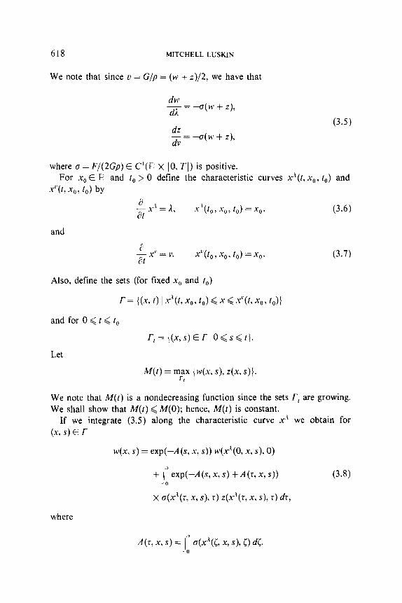
We note that since L’ = G/p = (~2 + z)/2, we have that

dw ~ = -a( 1%’ + z), d/l

(3.5) dz dv=c7(M1+Z),

where u = F/(ZGp) E C’(h X 10, TJ) is positive. For x,, E IF and t, > 0 define the characteristic curves x’(t, ?cO, to) and

xl’@, so, fo) by a ,x-t = 1 df ’

xyt,, x0, to) =x0, (3.6)

and

F , 27 x = “.

Xl’(f,) x0. to) = x0. (3.7)

Also, define the sets (for fixed x,, and to)

r = ((x, f) 1 xyt, x0, f,) < x < x”(f, xg, f,)}

and for 0 < t < f0

I-,= ((X,S)Er~O<s<f}.

Let

M(f) = mfx { W(X. s), Z(X, s)}.

We note that M(t) is a nondecreasing function since the sets Tr are growing. We shall show that M(f) <M(O); hence, M(f) is constant.

If we integrate (3.5) along the characteristic curve x.’ we obtain for (x, s) E l-

w(x. s) = exp(--A(s, x, s)) M~(x’(O, x, s), 0)

+ (_I exp(--A (s, x, s) + A (5, x, s)) -0

x a(x’(s, x, s), r) z(x’(r, x, s), r) dr,

(3.8)

where

GLOBAL SMOOTH SOLUTIONS 619

Hence

w(x, s) < exp(-A (s, x, s)) M(0) + [ 1 - exp(-A(s, x, s)) 1 M(s). (3.9)

Now suppose that (x, s) E r, and

w(x. s) = M(t).

Then from (3.9) we obtain

(3.10)

M(t) < exp(-A(s, x, s))M(O) + [ 1 - exp(-A(s, x, s))] M(t). (3.11)

Hence, since exp(-A(s, x, s)) > 0, we can conclude that M(t) < M(O). A similar argument applies when max,., z > maxr, MI. The proof is completed by applying the above arguments to (-w, -z). Q.E.D.

Now define

We can derive the following bound for o(t).

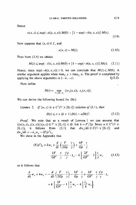
LEMMA 2. Zf (w, z) is a C’(R x [0, t]) solution of (3. l), then

D(t) < c + (b + 1) D(t) + aD(t)‘. (3.12)

Proof. We note that as a result of Lemma 1 we can assume that ((w(x, s), z(x, s)) I (x, s) E Ip x [0, t]} c f2. Let k = F’/2p. Since w E C’(R X

IO, rl>, it follows from (3.1) that dwddA E C(R X [O. t]) and dw,.dA = -A, w, - (F/p*)+.

We show in the Appendix that

(F/p’),=kw,+$ (&;)+$;

so it follows that

620 MITCHELL LUSKIN

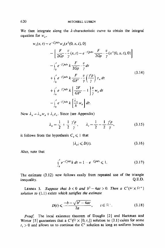
We then integrate along the l-characteristic curve to obtain the integral equation for w.~,

WJX, t) = e-s~kdTwv(XyO, x, I), 0)

- [ & * ; (x, t) - e -J-bkdr & ’ $ (x.‘(O, x, t), O)]

.f F - ! e-sikdr k---. - dz

-0 ~GP Y

+‘:*“‘k [p,] dr.

Now ,I, = &,,M’, + &z,. Since (see Appendix)

(3.14)

(3.15)

it follows from the hypothesis C, < 1 that

Also, note that

Stkdsk dr = 1 - e-sbkdr < 1. (3.17)

The estimate (3.12) now follows easily from repeated use of the triangle inequality. Q.E.D.

LEMMA 3. Suppose that b < 0 and 6’ - 4ac > 0. Then a C’(R x R ‘) solution to (1.1) exists which satisfies the estimate

D(t) < -b - \/b2 - 4ac

2a ’ ta?+. (3.18)

Proof: The local existence theorem of Doughs [2] and Hartman and Winter [5] guarantees that a C’(R x [0, tr]) solution to (3.1) exists for some 1, > 0 and allows us to continue the C’ solution as long as uniform bounds

GLOBAL SMOOTH SOLUTIONS 621

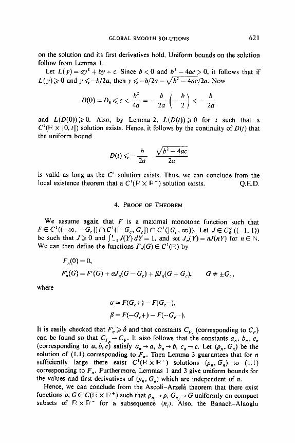
on the solution and its first derivatives hold. Uniform bounds on the solution follow from Lemma 1.

Let L(y) = a$ + by + c. Since b < 0 and b2 - 4ac > 0, it follows that if L(y) > 0 and y < -b/2a, then y < -b/2a - dm]2a. Now

O(O)=D,<c<$=-& -p <-& ( ) and L(D(0)) > 0. Also, by Lemma 2, L(D(t)) > 0 for r such that a C’(R X [0, t]) solution exists. Hence, it follows by the continuity of D(t) that the uniform bound

is valid as long as the C’ solution exists. Thus, we can conclude from the local existence theorem that a C’(R x R ‘) solution exists. Q.E.D.

4. PROOF OF THEOREM

We assume again that F is a maximal monotone function such that FE C’((-CO, -G,])n C'([-G,, G,])n C’([G,, CO)). Let JE C,“((-1, I)) be such that J>O and (\,J(Y)dY= 1, and set J,(Y)=nJ(nY) for nEN. We can then define the functions F,(G) E C’(lR) by

F;(G) = F'(G) + aJ,,(G - G,) + N,,(G + G,), G # *G,,

where

a = F(G,+) - F(G,-),

,8 = F(-G,+) - F(-G,-).

It is easily checked that FL > 6 and that constants C,” (corresponding to C,) can be found so that C,” + C,. It also follows that the constants a,, b,, c, (corresponding to a, b, c) satisfy a, -+a, b,+b, c,+c. Let @,,G,) be the solution of (1.1) corresponding to F,. Then Lemma 3 guarantees that for n sufficiently large there exist C’(R x R+) solutions (p,, G,) to (1.1) corresponding to F,. Furthermore, Lemmas 1 and 3 give uniform bounds for the values and first derivatives of (p,, G,) which are independent of n.

Hence, we can conclude from the Ascoli-Arzeli theorem that there exist functions p, GE C(R X R ‘) such that pnj+ p, G,,+ G uniformly on compact subsets of R x R + for a subsequence (nj). Also, the Banach-Alaoglu

622 MITCHELL LUSKIN

theorem implies that we may also assume that pnj - p, G,j - G weakly in W’*,X(ri x IF +). It is straightforward to show that

pt + G, = 0 a.e. @,t)E FI x iF+.

In order to demonstrate that

F(G) G, + (Gv), + P@), E - p a.e. (x, t) E IF X iFi +,

it is sufftcient to show that Fnj(G,i) - u weakly in L”‘(E X ip ‘) where aEF(G)a.e. (x,t)EIFxIR+.

We follow an argument due to Rauch [9]. Define the functions

F,(G) = ess sup F(Y). IF-Yl<c

&(G) = ess inf F(Y). IG-Yl<c

Let K be a compact subset of IR x iF +. Then for any E > 0 there is an )z,, > 4/s such that n > n, implies that 1 G(x, t) - G,(x, t)l < s/2 for (x, t) E K. Therefore,

Hence, if h E L’(K), h > 0, we have

j;. fi;(G) h dx df < I’, F,(G,) h d.u df < 1. F,(G) h du df. .h -K

Let n + co and use the weak convergence of F,(G,) to obtain

I’, &(G) h d,u dt < 1‘ ah dx df < I’ F,(G) h dx dr. -h .K .K

Next, use Lebesgue’s theorem above to let E + 0 and conclude that

1’ F(G) h dx df < 1. ah d.x dt ,< I’ F(G) h dx df, -K -K -K

where

E(G) = ‘,T E,(G) = F(G-), F(G) = ‘I$” F,(G) = F(G+).

GLOBAL SMOOTH SOLUTIONS 623

Since h > 0 was arbitrary, we can conclude that

E(G) < cr < F(G) a.e. (x, t) E K.

This concludes the proof of existence. We now turn to the proof of uniqueness. So, let Q1, G,) and (p2, Gz) be

two solutions of (2.7) in W”“O(lR X IF ‘), i.e.,

~;.t + Gi.x = 0 (x,t)E R x IF+,

Gi,, + (Y@i)’ - 0;) Pi..y + 2oiGi..y = ailPi* (4.1)

PiCx, O) = PO(*“)Y Gi(x, 0) = G,(x). XE P.

where ui E F(G,) a.e. (x, t) E IF x R +. Letting p’= p, - pz, G = G, - G2, we obtain from (4.1)

p; + e, = 0 (x, t) E R x p +,

G, + MPd2 - &?Y + 20, c

= [w2)2 - ~3 - (~cp,Y - ~31 P~..~ + 2h - 02) G?..,. (4.2)

-PA% - 021 - [PC’ - P?l 02.

m, 0) = 0, qx, 0) = 0.

Multiply the first equation in (4.2) by (Y@,)~ - oi)b and integrate over [-y, y] for y E IR + to obtain

1.’ /Tt/T[y@,)2 -E:] dx + I-’ &/7[y(pJ2 - u:] dx = 0. _ -Y . -.v

Hence. we obtain from integration by parts that

<K L? fy p” dx+ 0‘ G’dx

I - @[Y@,)~ - L’;] ’ , (4.3)

. -s -j

where K is a constant independent of t (since bi, Gi) E W’*s(R X Fi ’ )). Next, we obtain from multiplying the second equation in (4.2) by G and

integrating over [-y, y] that

=I.’ c’dx+(’ [y@,)2-c;]~Xi:dx+~y 2u$,Gd.u 2 dt._,t .-> . -j

<K p” dx + [’ c” dx p;’ [a, -a?] i:dx. (4.4) s

624 MITCHELLLUSKIN

It follows from integration by parts that

- jii2u,G,G~~=II,u,.,e2dx-v,2’ I’,.

Also, it follows from the monotonicity of F that

[o, - o2 1 G > 0.

Hence, we obtain from adding (4.3) and (4.4)

f 1.1” P”[~(JI,)~ - u:] dx + 1” c?‘dx] s --y

<K I--? I’)‘ p” d-Y + I-” G’ dx - [@[y@,)’ - u:] + G’v,] ’

,’ I . (4.5)

-Y

Now recall that the hypothesis b < 0 implies that y@i)’ - ut is positive and bounded away from zero. Also, note that the hypothesis bi, Gi) E W’*“(R x R+) guarantees that the boundary term in (4.5) is bounded independent of y, t E IF1 +. Hence, we can conclude from (4.5) and Gronwall’s lemma that for T > 0 we have @“, e) E L”(0, T; L’(lR)).

Next, since (~7, G) E W’.“(R x R+)nL”O(O, r,L’(lF?)), we can conclude that

G’[y(pJ2 - u:] + cT2u, (C, + 0 (4.6)

as y + +co uniformly for t E [0, T]. Thus, since p’(x, 0) = G(x, 0) = 0, it follows from (4.5), (4.6), and Gronwall’s lemma that p’= G = 0 for (x, t) E R x [0, r]. Finally, p’ = c = 0 in R X Rf since T > 0 was arbitrary.

Q.E.D.

5. AN EXAMPLE

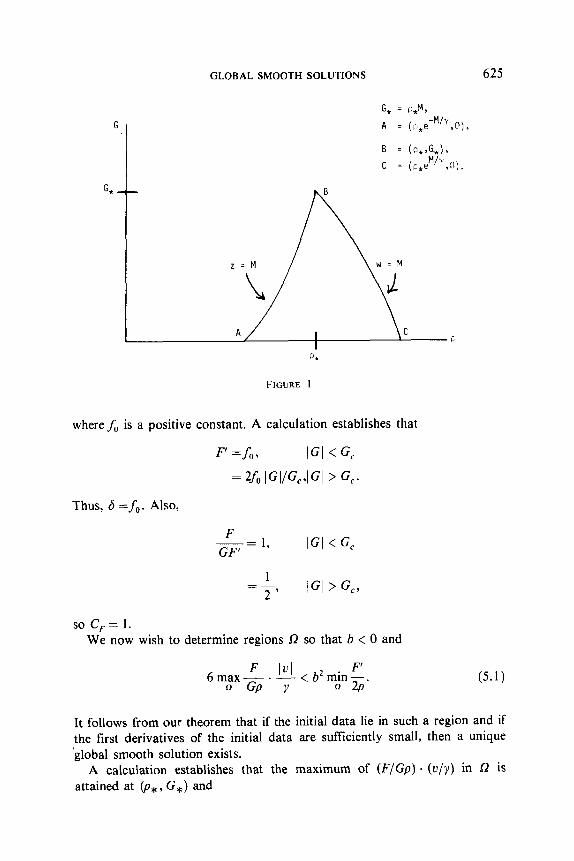
In this section, we present an example with a hypothetical friction factor which has been constructed to resemble the Moody friction factor [IO]. First, we assume that y@) is a constant and consider the structure of the invariant regions, R (see Fig. 1). It is easy to check that the curve z = M can be represented by the function G@) where G’ = y + u. Similarly, the curve w = M is represented by the function G@) where G’ = -y + u. For this example, C, = 0 and C, = max,(l u I/y) = M/y = G,/@, y).

Next, we consider the friction factor

F(G) =.L, G, IGI < G,

=fo IGI G/G,, IGI > Go

GLOBAL SMOOTH SOLUTIONS 625

G, = F*M,

G A = (~,e-~'~,@),

B = (P,>&),

c = (c*lP" ,3).

G, m-

FIGURE I

wheref, is a positive constant. A calculation establishes that

F’ =fo, IGI < G,

= X3 lGI/GJGl > G,.

Thus, 6 =fO. Also,

F -= 1, GF’ ICI < G,

1 2’ IGI > Go

so c,= 1. We now wish to determine regions R so that b < 0 and

(jmax-!?-.!d<b2minF’ R GP Y R 2p’ (5.1)

It follows from our theorem that if the initial data lie in such a region and if the first derivatives of the initial data are suffkiently small, then a unique ‘global smooth solution exists.

A calculation establishes that the maximum of (F/Gp) . (u/y) in R is attained at @*, G,) and

626 MITCHELL LUSKIN

F ly f, C, -.- maXn Gp y=p*

foes G, =-.- pz+ G,

if G, < G,

if G, > G,.

To see this. note that

F c f, c foG -.- Gp I,=y;=T if G <G,

fo fo G2 =--D* x-T )‘G, YG, P

if G>G,.

Thus, it is easy to see that the maximum of (F/Gp) . (u/y) on R lies on the curve z = M. Now if z = M is represented by the function G@) such that G’ = y + 19, we see that

(4!2&‘~~[~]=~[~]>0,

(~$q’=~[2~G~3-G2]=&[y >o.

Hence, the maximum is taken at the point B = @*, G,). Also, it is easy to check that the minimum of F’/2p in R is attained at @*e”U’; 0) and

. F' f, -c', m;nZp=2p,e .

Thus, (5.1) is equivalent to

and

1 < (I-- CA’ e-“‘ 12c,

if G,<G,

(1 - Cd’ e-c’ 12Cf

if G,>G,.

So, consider the curve defined by the relation

1 = (1 - CA2 e-L‘S 12c,

if G < G,

and YP -= Gc

(1 -Cs)' e-C' 12Cf

if G>G,.

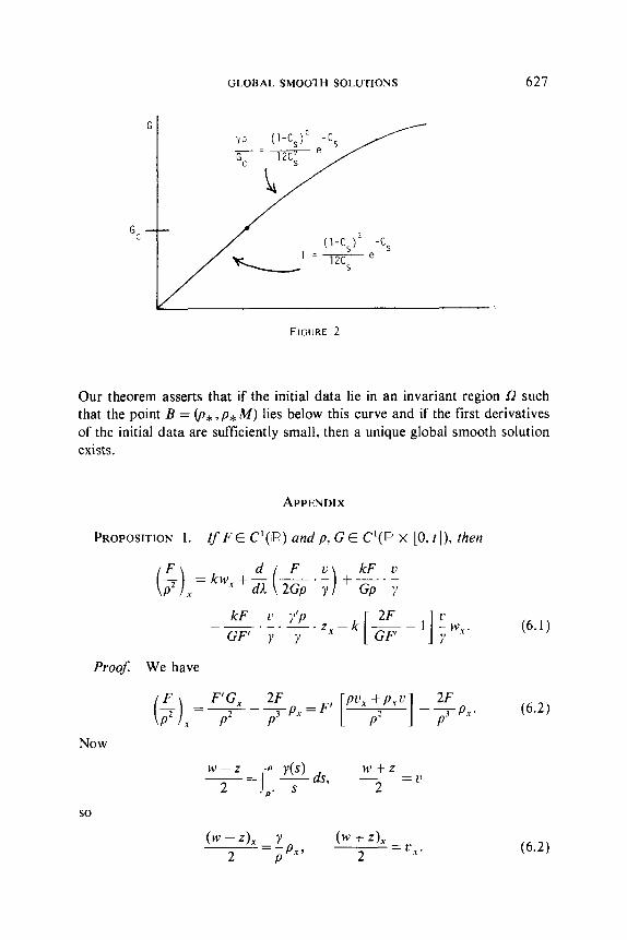
GLOBAL SMOOTH SOLUTIONS 627

FKXJRE 2

Our theorem asserts that if the initial data lie in an invariant region f2 such that the point B = @*,p*MM) lies below this curve and if the first derivatives of the initial data are sufficiently small, then a unique global smooth solution exists.

APPENDIX

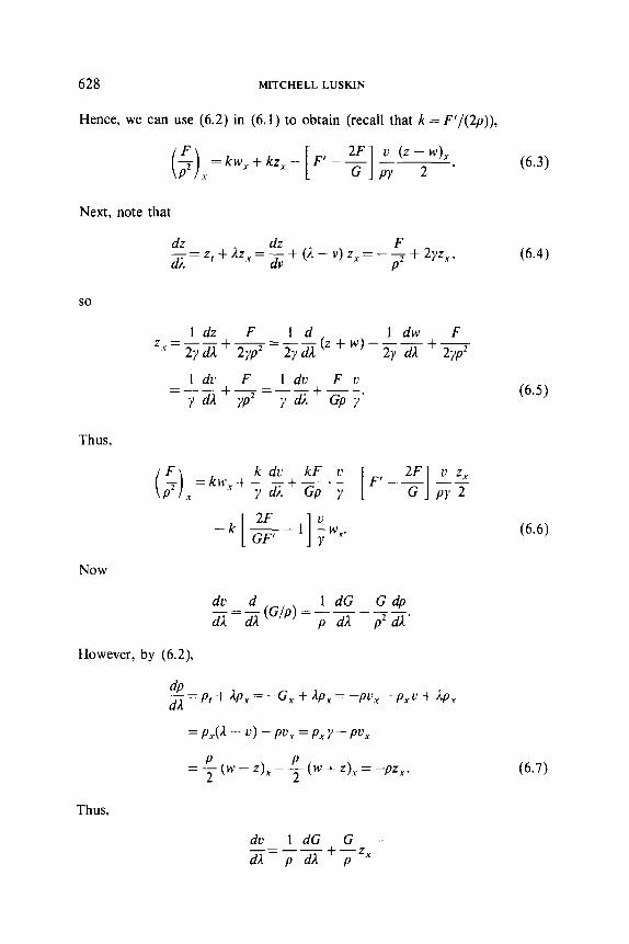
PROPOSITION 1. Zf F E C’(IR) and p, G E C’(IF: x [0, tl), then

kF ~1 y’p --.---.z.,-k[g-l];t,y (6.1)

GF’ y y

Proof: We have

F F’G, 2F (-) =T-Tpx=F’ [pux;p~v”] -+. P2r P

(6.2) P

Now

M’ + z - = p 2

so

(W--L), Y 2 =pP.TV

(w + ZL = c 2 x* (6.2)

628 MITCHELL LUSKIN

Hence, we can use (6.2) in (6. I) to obtain (recall that k = F’/(2p)),

Next, note that

dz dz F

dA -=zr,+~z,=~+(~-V)zX=-p2-+2yZ_r,

1 dty =--+F=Idc+Lv YdA YP’ Y& GP Y’

Thus,

Now

dv d ,=-&G/p,=+:-;;.

However, by (6.2),

dp ~=P,+~“=-G,+~P,=-pu,-p,c+~p,

= P,(l - u) - PO, = P+ Y - Pt’x

= $ (w - z)x - $ (w + z)x = -pz, .

(6.3)

(6.4)

(6.5)

(6.7)

Thus,

dv 1dG G ~=p~+p

GLOBAL SMOOTHSOLUTIONS 629

and by (6.7)

k dv F’ dG kv --= Y dl 2p2yz+yzx

1 d =T-F+?r,

2~ Y dA

(6.8)

The estimate (6.1) now follows from substituting (6.8) in (6.6). Q.E.D.

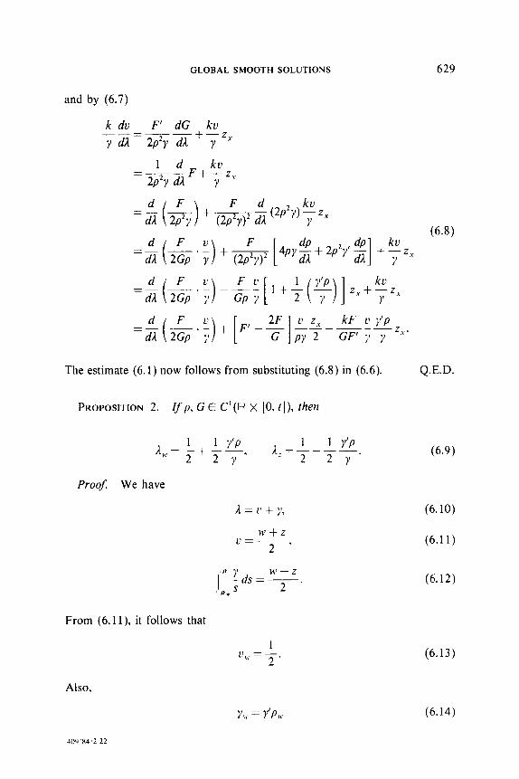
PROPOSITION 2. f'p, GE C'(IR x [0, I]), then

Proof. We have

Also.

4oq ‘84 ‘2 22

From (6.11). it follows that

Yw = Y'P,,

(6.9)

(6.10)

(6.1 1)

(6.12)

(6.13)

(6.14)

630 MITCHELL LUSKIN

and from differentiating (6.12) with respect to W,

P,cY 1 -=-. P 2

Thus. we obtain from (6.14) and (6.15)

Y'P Y,,. = 2y'

(6.15)

(6.16)

The first relation in (6.9) now follows from (6.13) and (6.16). The second relation in (6.9) is proved similarly. Q.E.D.

REFERENCES

I. K. CHUEH. C. CONLEY. AND J. SMOLLER, Positively invariant regions for systems of non- linear diffusion equations, Indiana Univ. Math. J. 26 (1977), 373-392.

2. A. DOUGLIS. Some existence theorems for hyperbolic systems of partial differential equa- tions in two independent variables, Commun. Pure Appl. Mafh. 5 (1952), 119-154.

3. T. DUPONT, Galerkin methods for modeling gas pipelines, in “Constructive and Com- putational Methods for Differential and Integral Equations,” Lecture Notes in Mathematics No. 430. Springer-Verlag, Heidelberg, 1974.

4. T. DLIPONT. Decay properties of some pipeline flow equations, preprint. 5. P. HARTMAN AND A. WINTER, On hyperbolic partial differential equations, Amer. J.

Math. 74 (1952). 834-864. 6. P. LAX, Development of singularities of solutions on nonlinear hyperbolic partial differen-

tial equations, J. b~‘ath. Phw. 5 (1964), 61 l-6 13. 7. M. LUSKIN. A finite element method for first order hyperbolic systems. Marh. Camp. 35

(1980). 1093-I I I?. 8. T. NISHID.~. Quasilinear wave equations with the dissipation. Publ. Math. Orsa!, ( 1977). 9. J. R.x~cH. Discontinuous semilinear differential equations and multiple valued maps.

Proc. .4mer. hlarh. Sot. 64 (1977). 277-282. IO. 1’. STREETER. “Fluid Mechanics.” 5th ed.. McGraw-Hill, New York. 1971.